Article

Hybrid Statistical Testing for Nuclear Material Accounting Data and/or Process Monitoring Data in Nuclear Safeguards

1
Statistical Sciences, F600, Los Alamos National Laboratory, Los Alamos, NM 87545, USA
2
Systems Design and Analysis, C921, Los Alamos National Laboratory, Los Alamos, NM 87545, USA
*
Author to whom correspondence should be addressed.
The authors contributed equally to this work.
Energies 2015, 8(1), 501-528; https://doi.org/10.3390/en8010501
Submission received: 13 November 2014 / Accepted: 15 December 2014 / Published: 13 January 2015
(This article belongs to the Special Issue Advances in Nuclear Reactor and Fuel Cycle Technologies)

Abstract

:
The aim of nuclear safeguards is to ensure that special nuclear material is used for peaceful purposes. Historically, nuclear material accounting (NMA) has provided the quantitative basis for monitoring for nuclear material loss or diversion, and process monitoring (PM) data is collected by the operator to monitor the process. PM data typically support NMA in various ways, often by providing a basis to estimate some of the in-process nuclear material inventory. We develop options for combining PM residuals and NMA residuals (residual = measurement − prediction), using a hybrid of period-driven and data-driven hypothesis testing. The modified statistical tests can be used on time series of NMA residuals (the NMA residual is the familiar material balance), or on a combination of PM and NMA residuals. The PM residuals can be generated on a fixed time schedule or as events occur.

1. Introduction and Background

Nuclear material accounting (NMA) is a component of nuclear safeguards, which are designed to detect illicit diversion of special nuclear material (SNM) from the peaceful fuel cycle to a potential weapons application. NMA consists of periodically comparing measured SNM inputs to measured SNM outputs, and adjusting for measured changes in inventory. Process monitoring (PM) data is a relatively recent component of safeguards that is collected more frequently than NMA data. PM data is often only an indirect measurement of the SNM, or is a direct measurement of bulk mass that includes SNM and non-SNM. PM data is typically used as a qualitative measure to supplement NMA, or to support indirect estimation of difficult-to-measure inventory for NMA [1,2,3,4,5,6,7,8,9,10,11,12].
Nuclear safeguards are applied at all stages of the nuclear fuel cycle, from uranium conversion to SNM waste disposition. To focus this article, we only discuss reprocessing facilities. Traditional NMA at large reprocessing facilities closes the material balance (MB) approximately every 10 to 30 days around an entire material balance area, which typically consists of multiple process stages. 
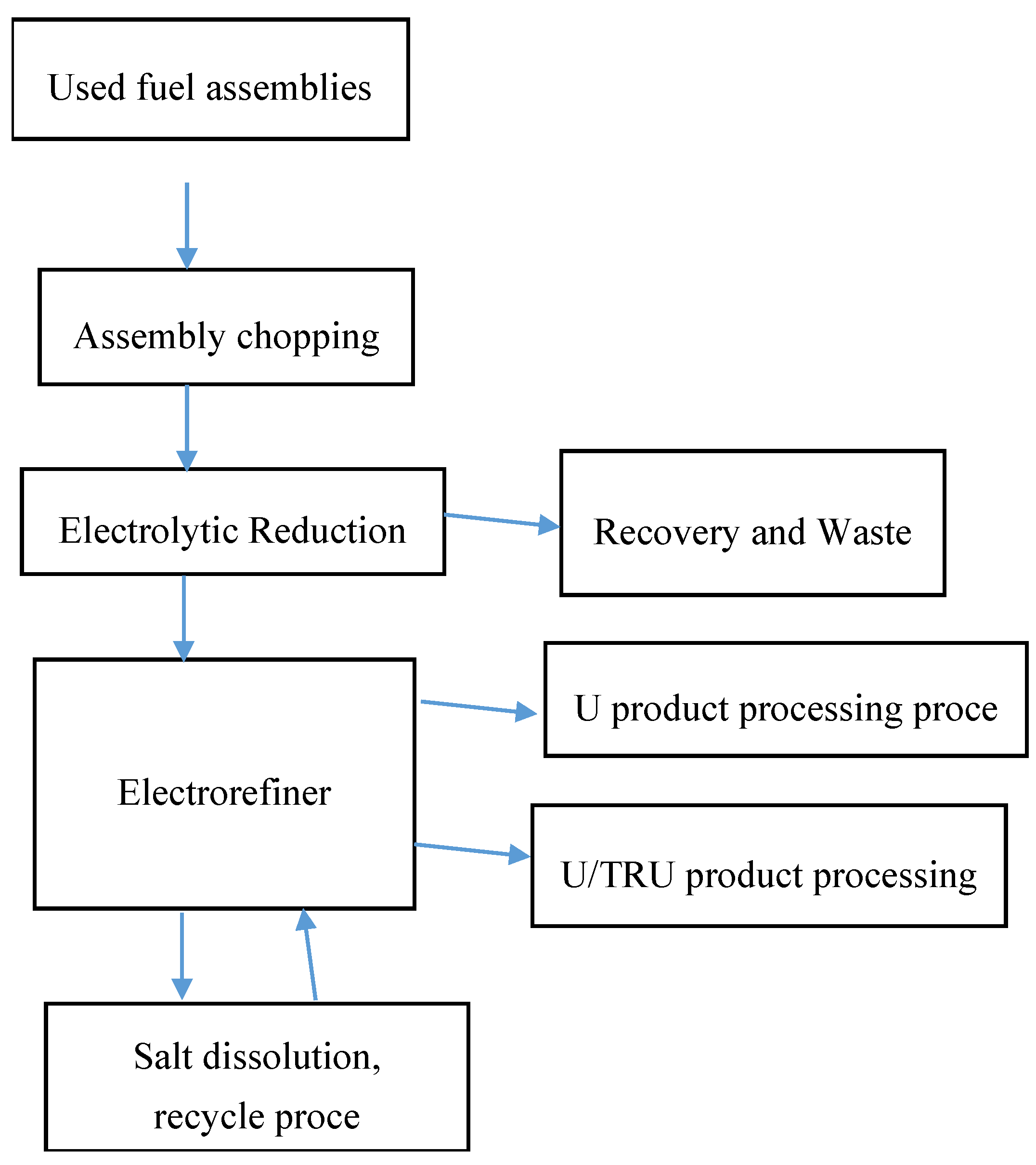
Figure 1 is a picture of SNM flows at a generic electrochemical reprocessing facility [13,14,15,16,17,18,19], which is anticipated to have large SNM throughput but much less processing equipment than a similar-throughput aqueous reprocessing facility [7,8,9]. Both PM and NMA measurements are available at aqueous and electrochemical reprocessing facilities. An electrochemical facility operates mostly in “batch mode”, such as batches of product baskets taken from the electrorefiner (Figure 1). An aqueous facility has tanks and processes in both batch and continuous operation (the chemical separations vessels operate in continuous mode, so some tanks ship and receive continuously from the separations vessels).
Our proposed options to quantify the benefit of using both PM and NMA data define the system alarm probability as the conditional probability of an alarm given the true model parameters (such as the true SNM loss in each vessel over a specified time), denoted P(alarm|diversion scenario). We assume there are time series of p residuals r1, r2, …., rp, which include MBs from NMA, plus residuals generated from PM data. In both PM and NMA, a residual is computed as residual = measurement − prediction. The prediction can come from an engineering model or from purely empirical means on historical training data that is assumed to not contain SNM diversion. The probability P(alarm|diversion scenario) is a function of the true states of nature (which depend on whether SNM has been misdirected), the measurement system, the PM residual streams in use, and the alarm rule(s).
It has long been believed that PM can improve domestic and international safeguards; although the cost to the safeguards budget is relatively low because PM data is already being collected by the operator, PM benefits are difficult to quantify. This paper uses PM residuals as a simple extension of NMA to quantify PM benefits. One key assumption is that the safeguards approach includes model-based predictions that can be compared to corresponding measurements, resulting in time series of residuals. The requirement for high-quality predictions leads to technical challenges in safeguarding either aqueous or electrochemical reprocessing facilities. For example, there is ongoing work aimed at high-quality modeling of the electrorefiner in an electrochemical facility [17]. Strictly speaking, our approach leads to high SNM loss detection probability (DP) only for the specified diversion routes; however, there is also high loss detection probability for any type of abrupt loss. See Appendix 2 for more detail. Also, in the context of international safeguards, there is not yet an approach to authenticate operator PM data; authentication will depend on facility type and is under investigation.
The following sections include a description of NMA and of PM, pattern recognition, model-based prediction, discussion of simulated data, extensions to include additional PM residuals, example of combining PM and NMA data, and a summary. The simulated numerical example that combines NMA and PM data includes daily PM data from 13 vessels, including one input, eight inventory vessels, and four output vessels. PM data from each vessel consists of a time series of residuals. The overall MB can be computed at any desired frequency of 1 day or longer. Reference [1] reviews related work in the nuclear safeguards and statistics communities.
Figure 1. Generic electrochemical reprocessing facility with key activities shown.
Energies 08 00501 g001

2. NMA and PM

While NMA estimates SNM mass balances and uncertainties, PM sometimes tracks SNM attributes qualitatively or in the case of solution monitoring, might track bulk mass and volume. PM data can also include very frequent high-dimensional spectral data from gamma detectors [20,21,22], or low-dimensional flow and/or in-tank volume data from flow meters or in-tank dip tubes. In some cases, PM data can be relatively high quality, such as in-line mass or volume flow measurements, and some current research is aimed at high-quality in-line SNM accountability measurements for electrochemical facilities [14,15,16,17,18,19] and aqueous facilities [7,8,20,21]. The next two subsections briefly describe NMA and PM. See Appendix 1 for more detail on NMA and PM.

2.1. NMA

In NMA, the MB is defined as MB = Ibegin + Tin − Tout − Iend, where Tin is transfers in; Tout is transfers out; Ibegin is beginning inventory; and Iend is ending inventory. The measurement error standard deviation of the MB is denoted σMB. The key quantities in NMA are the MB and its measurement error standard deviation σMB. If the MB at a given time (“balance period”) exceeds k σMB with k in the 2-to-3 range, then the NMA system “alarms”. Considerable effort is aimed at assessing measurement uncertainties to estimate σMB [23,24]. Choosing k in the 2-to-3 range for a low false alarm probability is based on an appeal to a central limit theorem effect arising from combining many measurements to justify assuming the measured MB is approximately Gaussian distributed around the true MB [10,12,23].

2.2. PM

PM is a broad term that in nuclear safeguards includes monitoring by radiation detectors, cameras, and monitoring solutions in vessels using pressure-sensing dip tube or other technology (which is this article’s focus).
PM often enables a type of frequent NMA, which is usually referred to as near real time accounting (NRTA). NRTA is typically described as: frequent balance closures based mostly on measurements of the shipments and receipts, with varying capability to measure or estimate in-process inventory. In practice, “frequent” is typically daily or weekly (however, PM-based balance closures are common on a per-batch basis which could be daily or multiple times per day). Facilities that close balances very frequently, such as daily or after each batch transfer, rely on various shortcuts or partial measurements. For example, it is rare to equip each processing unit with in-line holdup or in-process inventory monitors. Therefore, either engineering estimates, or historical by-difference estimates are used for negotiated portions of the in-process inventory measurements [25]. In the NRTA scheme at the THORP (“thermal oxide reprocessing plant”) in England [26], full material balance closures are not as often as weekly because of the infrequency of Pu concentration measurements. Full balance closures are less often than weekly, but pseudo-balance closures using empirical relations to estimate the Pu concentration are quite frequent (roughly daily). Although in-line dip tubes measure vessel volume every few seconds, there might not be a capability to measure the Pu concentration in-line. In-line dip tubes estimate solution density, so empirical relations together with the density estimate can infer (but not directly measure) the Pu concentration [27]. An NRTA system that measures all material is preferred, but even the best system will typically rely on partial measurements and/or engineering estimates for at least part of the in-process material [1,7,25].
PM can potentially have high SNM loss detection probability for abrupt diversion. Reference [27] showed that SNM loss during tank “wait modes” would be much easier to detect than SNM loss during “transfer modes” (see Section 3). This is largely due to canceling systematic errors when two level measurements in the same tank are compared. If we need high confidence in PM only during transfer modes, this is a potential savings. However, because there is no in-line Pu concentration measurement, there are spoof scenarios. The adversary could divert without an alarm during a wait mode by replacing the removed volume with the correct density solution. If this occurred over a one day period (the daily Pu throughput is approximately 50 kg), then downstream Pu concentrations could be back at expected values by the next monthly balance closure when Pu concentrations are measured in all key tanks. Short-cut assay methods such as a volume and a calculated SNM concentration do not directly measure the SNM of interest but are often used for some of the measurements in frequent NMA (such as every 10 days). PM directly supports NMA if PM is used to estimate holdup [1,28,29]. Currently, there is no attempt to quantitatively use PM to meet detection probability goals.

3. Flow Rate Monitoring and Event Marking

Raw solution monitoring (SM) data are unlikely to be useful as input features for pattern recognition. Instead, raw SM data can be parsed into key events such as shipments and receipts, as done by some SM evaluation systems [4,6,27]. This allows one to regard each tank as unit process area and generate residuals that are analogous to the MB from NMA. Alternatively, flow rates to and from tanks can be used to generate very frequent (every few minutes or hours or days) residuals from each tank, without event marking [30]. The flow rate monitoring option is known [30] to have challenges, including the following: flow rates can be difficult to measure; in-vessel measurements are unstable if the vessel contents are rapidly changing; synchronization errors arising from flow rate changes that occur at unknown times between the recorded data times; serial correlation in MBs due to successive residuals sharing the same estimation error effects, and larger data dimension than using residuals from marked events. For example, 
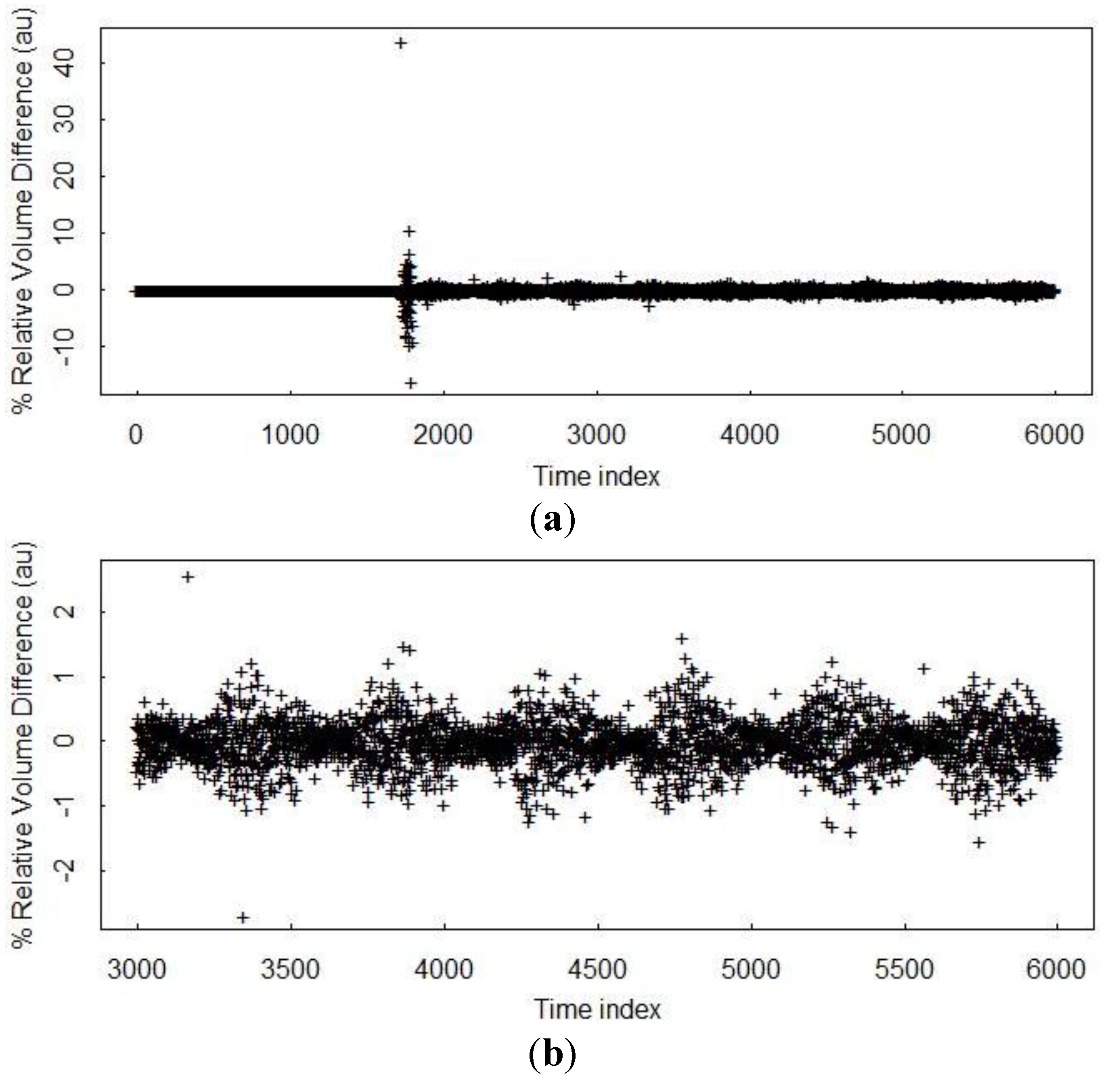
Figure 2 plots simulated bulk volume balance in one tank from the safeguards system performance model (SPM) [30] before the effects of measurement errors are introduced. There is a large transient volume balance near 1700 min that masks the −1 to 2 percent relative volume balance that persists for the entire simulation.
Figure 2. Illustration of synchronization error in an aqueous tank modeled in the System Performance Model (SPM). In (a), the synchronization error is present but a large volume residual occurred at the beginning of material flow near minute 1700 so synchronization errors are almost not visible. In (b), a relatively short section of time is plotted, and synchronization error is approximately a −1 to 2 percent effect (in arbitrary units, au, because this is percent relative change).
Energies 08 00501 g002
These −1 to 2 percent relative volume balances are due to flow changes occurring at slightly different times than the times that the simulation records data, which we call a synchronization error. Synchronization errors also occur in real facility data, so there has not been an attempt to remove them from simulated data. 
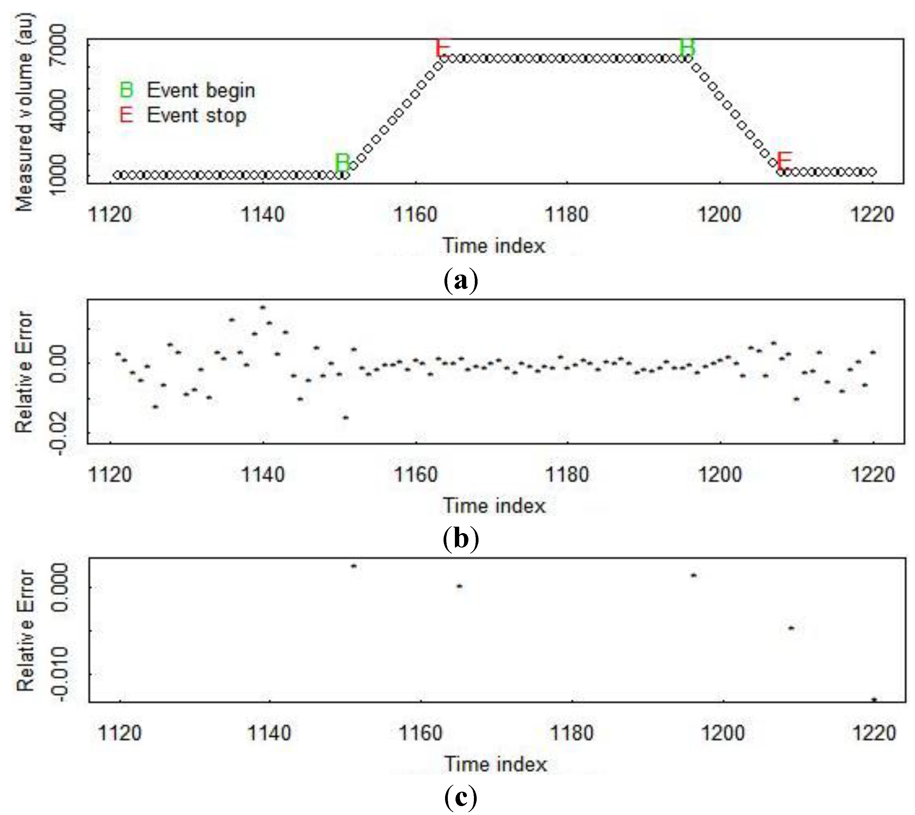
Figure 3 illustrates PM residuals from two options. Option 1 assumes flow rates are measured and that PM residuals can be generated on a fixed schedule, such as every 6 min, every hour, or every day [30]. Option 2 uses event marking and so parses each vessel into wait and transfer modes [1,4,6,27]. Note that option 2 results in only 5 residuals while option 1 results in many more residuals over the same time period.
Figure 3. (a) The measured volume in a tank during a receive, wait, ship cycle; (b) PM residuals for bulk volume using option 1 PM; (c) PM residuals for bulk volume using option 2 PM. In PM option 1, residuals are generated on a fixed time schedule. In PM option 2, residuals are generated at the end of each “wait” and “transfer” mode, and transfer-mode residuals compare the bulk volume change in the shipper tank to the corresponding change in the receiver tank.
Energies 08 00501 g003

4. Model-Based Predictions

In NMA, the MB concept is based on a simple model of mass conservation which implies that the true MB should be zero. In PM, both first-principles and empirical models can be used to predict SNM mass in a given location. Also, models for how one might misdirect Pu can suggest what observables would be generated. For example, [3] describes a simple model of the dissolver vessel in the head-end of an aqueous reprocessing plant. Excess Pu can be directed to the waste hulls by incomplete dissolution using off-normal nitric acid concentration and/or off-normal dissolver batch cycle times. In the example in [3], PM data includes cycle times, temperatures, and acid concentrations, that are all inputs to the example’s model of dissolver operation, and so the PM data enabled a model-based prediction of the Pu in the hulls. This model-based prediction can provide the basis for having a PM residual associated with each batch of hulls, defined as residual = measurement − model prediction. Currently, a neutron-based hull monitor is used, but the hull monitor measurement is not compared to a model prediction. This article assumes that such a PM scheme is feasible, and provides a way to monitor for diversion to the hull waste stream.
PM (extended, if needed, beyond in-tank level, density, and temperature to include flow measurements and/or in-line Pu concentration measurements) can help provide a predicted or book value for waste streams. For example, recall that [3] describes a model for the head end of an aqueous reprocessing plant that results in a model-based prediction (or “book value”) of the Pu mass in the hulls waste stream. Xerri et al. [31] distinguish holdup from “hidden inventory” and use by-difference PM data to estimate holdup. Assuming that diversion of excess Pu to the hulls is the only credible diversion route in the head end, it is valuable to have such a “model-based” prediction of the Pu in each hull batch that relies on easily measured quantities such as dissolver cycle time, temperature, and feed nitric acid concentration or bulk density.
Similarly, pulsed column models [25] can provide a book value for effluent streams (an example is given in [1]). For electrochemical facilities, a few models of the electrorefiner are being developed that would generate time series of PM residuals [15,16,17,18,19]. The intent is to detect off-normal conditions that could indicate misdirection of Pu. Monitoring such profiles can lead to residuals as we have described for simpler models involving mass and/or volume balancing of SM data for each key process tank.
Model-based predictions as just described can provide a new way for PM plus NMA to detect diversion on the basis of monitoring the corresponding residuals. A key fact is that diversion to streams that should have relatively small amounts of Pu can be easily detected provided frequent PM data is available, and the model-based predictions are reasonably high quality (i.e., have low total error variance; see Section 8).

5. Data Fusion

In NMA, diversion DP is the safeguard’s system main figure of merit for a specified diversion amount and time frame. Because σMB determines the DP [12], via the assumed Gaussian distribution of the MB, efforts are continually made to reduce σMB. In combining PM data with NMA data, we propose to retain diversion DP as the figure of merit, but extend the diversion scenario description from SNM amount and time frame to include how the SNM is diverted. A key task is then to estimate the probability distribution of the combined PM and NMA residuals in the no-diversion case and in the diversion case. The residual probability distribution in the no-diversion case can be estimated by analysis of real facility data, and in the diversion case can be estimated by modeling and simulating the effects of facility misuse on real data [1,22]. See Appendix 2 for more detail on data fusion.

6. Hybrid of Period-Driven and Data-Driven Pattern Recognition

Suppose NMA and PM residuals are evaluated frequently (such as every day or every 10 days), but a statistical decision is made every year, to alarm or not. Yearly decisions are practical in safeguards because facilities often schedule a partial shutdown and clean out of the facility, which provides a convenient time to have most SNM in relatively easy-to-measure forms. This is a hybrid of both period-driven and data-driven statistical evaluation. See Appendix 2 for more detail on period-driven and data-driven pattern recognition. Appendix 2 illustrates that current detection probabilities based on period-driven statistical testing are decreased if the adversary diverts across multiple time periods; therefore, some combination of period-driven and data-driven pattern recognition using statistical testing is desired.

7. Pattern Recognition

In a typical pattern recognition problem, the data consist of n cases of (y, X) pairs where the integer y ϵ (1, 2,..., J) is the class and X is a p-dimensional predictor vector. The goal is to use X to predict the class y, and this task is sometimes called classification, discriminant analysis (DA), or supervised learning. Regarding notation, vectors and scalars can be distinguished by context and definition. For example, y is a scalar and X is a p-dimensional vector. See Appendix 2 for more detail on pattern recognition for combining NMA and PM data.

8. Example

We consider an material balance accounting (MBA) with 13 vessels, including one input, eight inventory vessels, and four output vessels. 
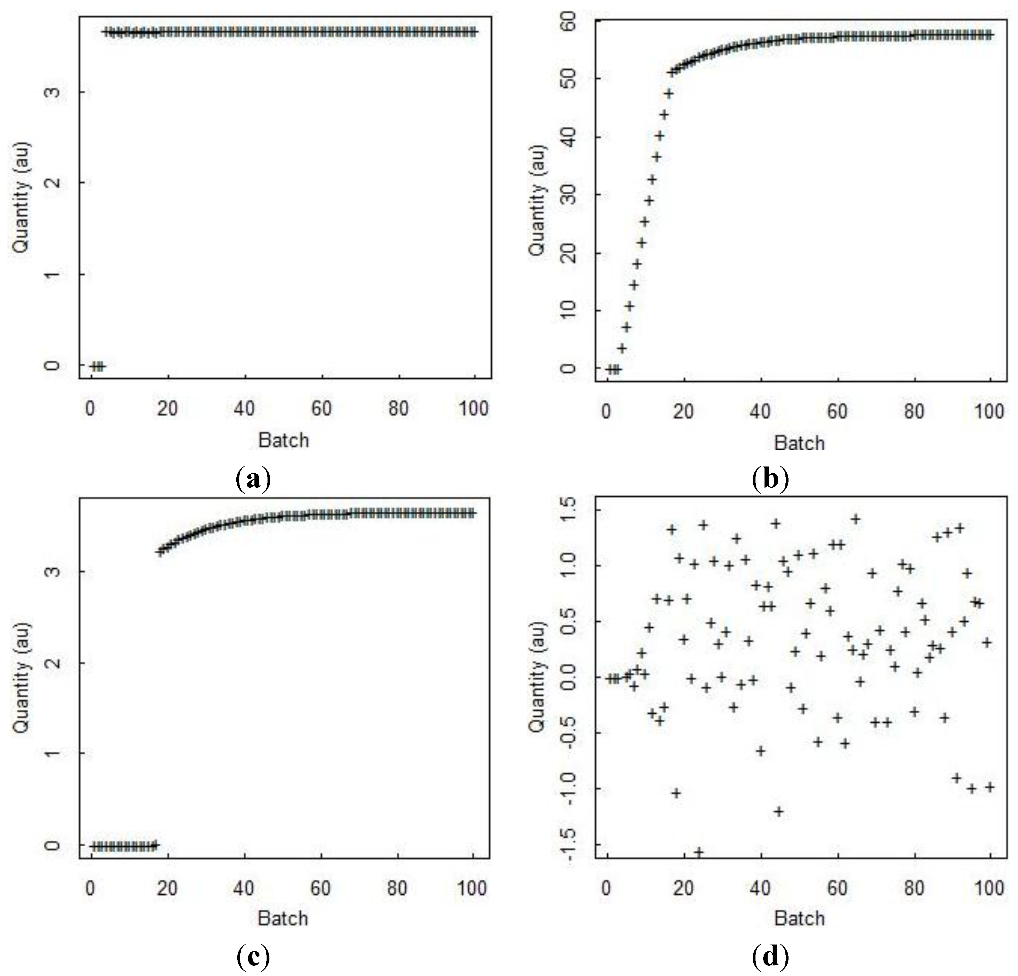
Figure 4 is simulated input, output, and inventory bulk mass data from a generic electrochemical reprocessing plant provided by Sandia National Laboratories from the SPM [14]. Because there is far less experience with electrochemical reprocessing than with aqueous reprocessing, we are not in position to have a defensible estimate of measurement error variances. So, purely for illustration purposes, we assume 1% relative random error standard deviation on all measurements, and 0.5% relative systematic error standard deviation on all measurements (these are somewhat larger than typical values in aqueous reprocessing [24]).
A time series of 100 simulated MBs (with measurement errors of 1% relative random error standard deviation and 0.5% relative systematic error standard deviation) in arbitrary units (au) is also shown in Figure 4d for each time step.
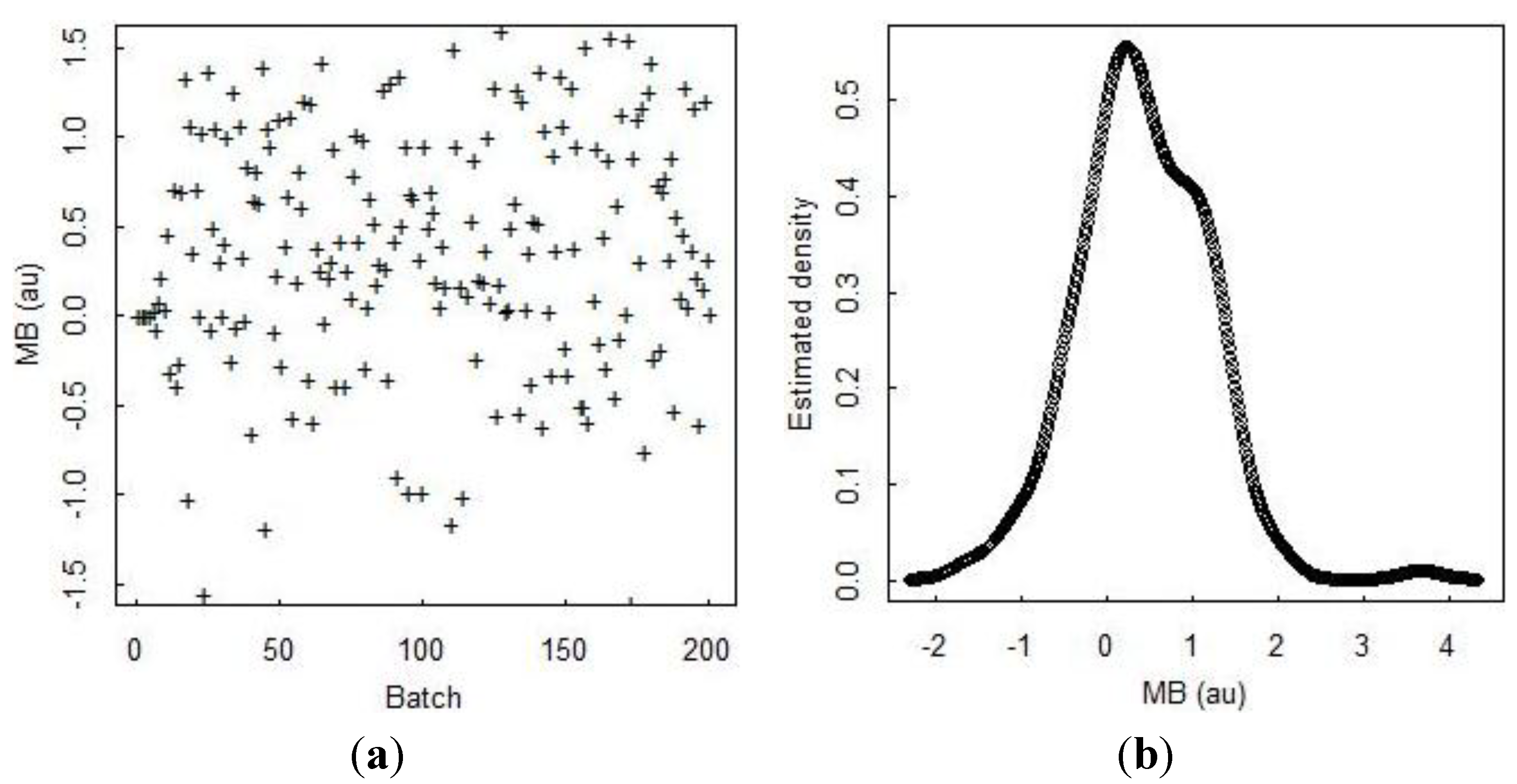
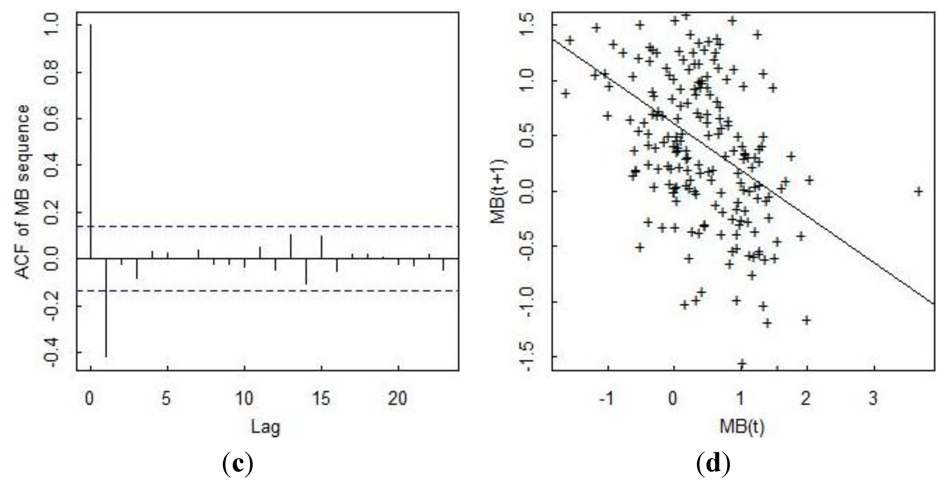
Figure 5 plots 200 MBs that are computed each day rather than each time step (so the values are somewhat different) in (a), the estimated probability density of the MB value in (b), the autocorrelation function (ACF) of the MB sequence in (c), and a lagged plot of the present MB versus the previous MB in (d). The strong lag-one ACF in (c) indicates that the inventory measurement error is non-negligible. The variance of the MB sequence quickly increases to its stationary value, as evident from the scatter increasing in (a) from an initial small value to a larger stationary value as inventory vessels reach capacity later in the simulation.
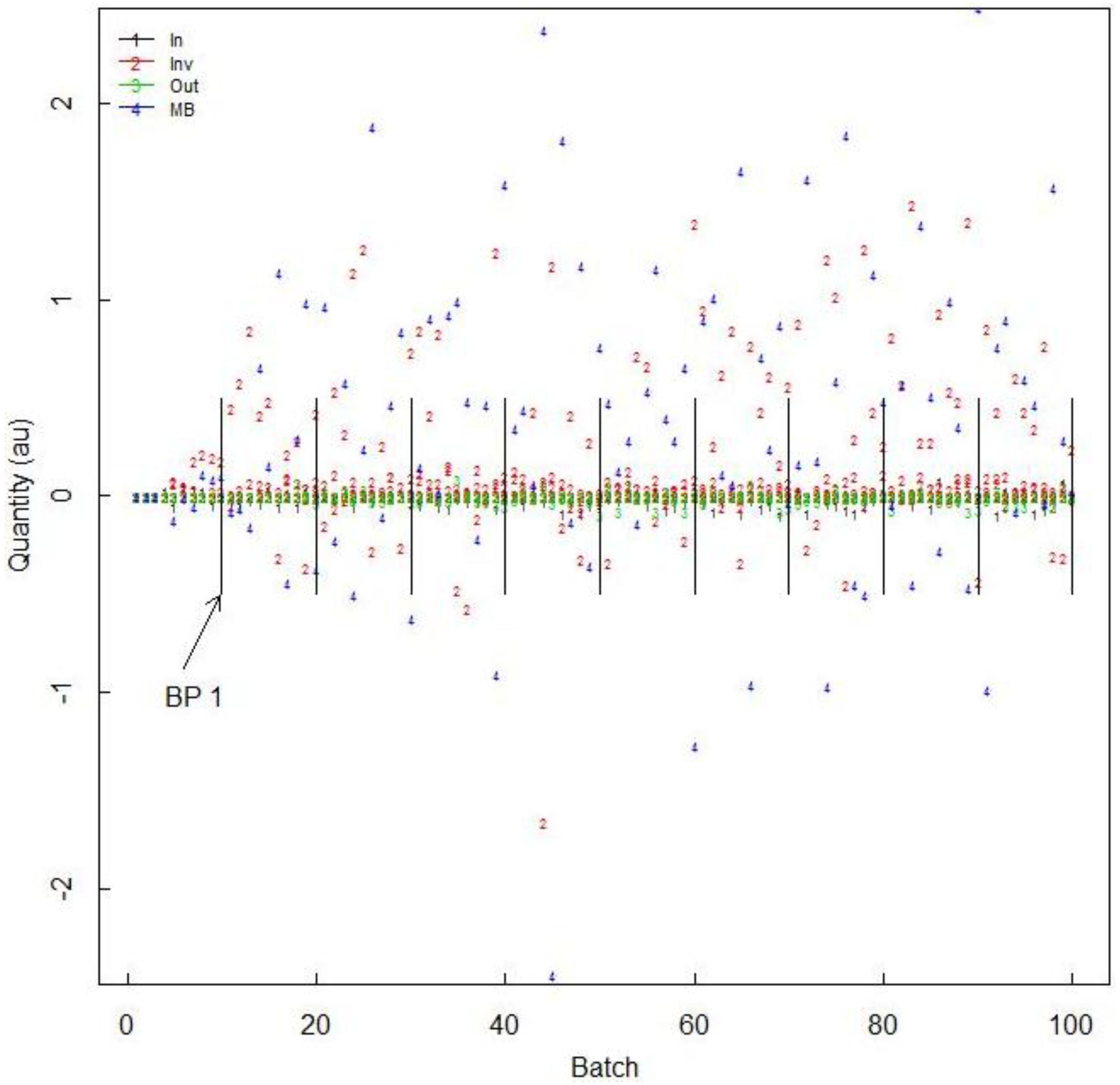
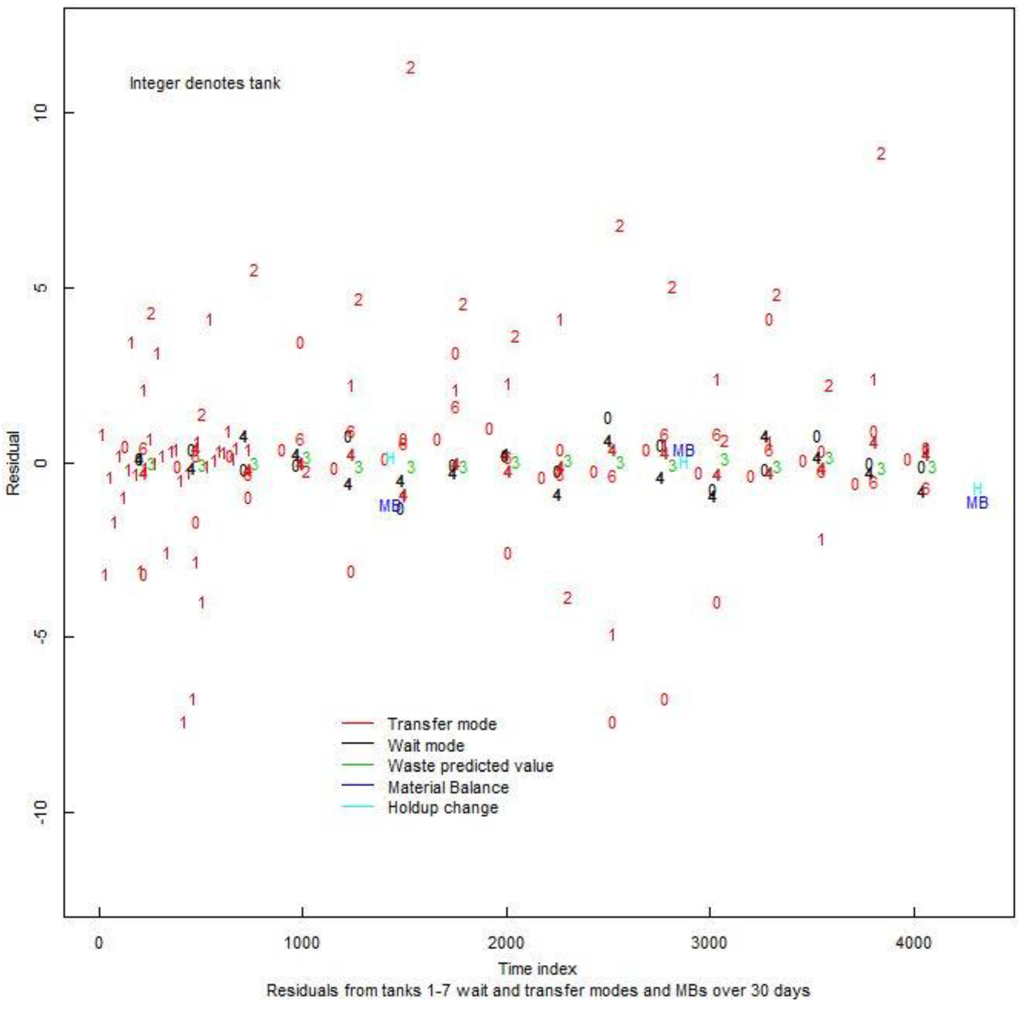
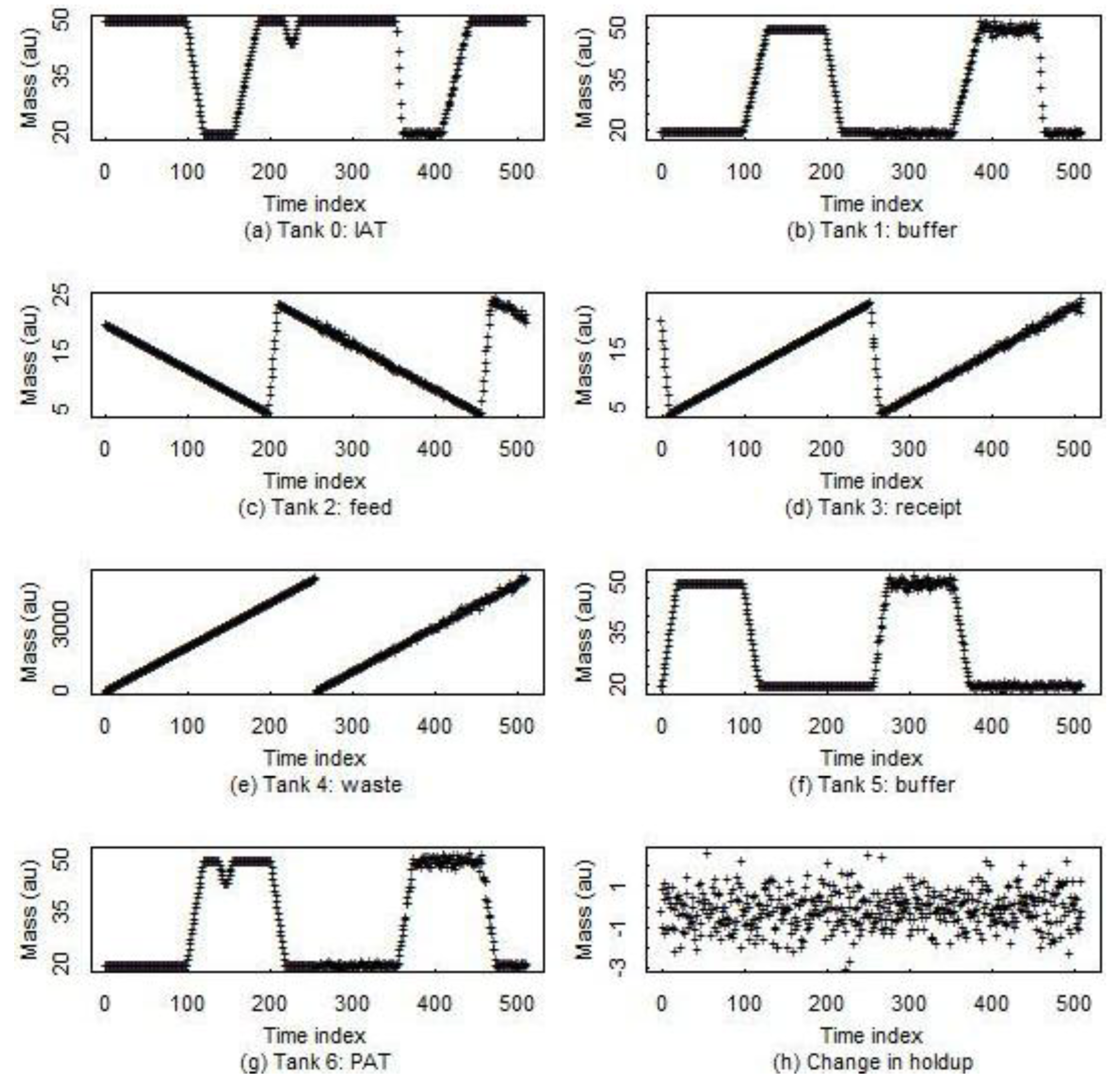
Figure 6 plots the 14 daily residuals (one input, eight inventory, four outputs, and one MB). For comparision, Figure 7 and Figure 8 are for a 7-tank MBA at an aqueous facility described in [1].
Figure 4. (a) Daily total input; (b) total inventory in eight vessels; (c) total output from four streams; and (d) daily (“batch”) MB in generic electrochemical data simulated from the SPM.
Energies 08 00501 g004
Figure 5. Daily material balances (“batches”) in (a); the estimated probability density of the MB value in (b); the autocorrelation function of the MB sequence in (c); and a lagged plot of the present MB versus the previous MB in (d).
Energies 08 00501 g005aEnergies 08 00501 g005b
Figure 6. Daily residuals from the one input, from each of the eight inventory vessels, from each of the four output vessels, and the daily MB. We also consider less frequent BPs, every 10 days.
Energies 08 00501 g006
Figure 7. Example data from a 7-tank aqueous facility MBA. Some tanks are batch input, batch output (denoted B/B). Tanks that are just upstream or downstream from a separations vessel have a continous (C) mode. (a) Input accountability tank; (b) Buffer tank; (c) Feed tank; (d) Receipt tank; (e) Waste tank; (f) Buffer tank; (g) Output accountability tank; (h) Change in holdup.
Energies 08 00501 g007
Figure 8. Residuals from PM and NMA for the 7-tank MBA in an aqueous facility. The PM residuals occur at the end of each wait event and after each transfer event. The NMA residuals are the usual MBs every 10 days.
Energies 08 00501 g008
We return now to the electrochemical example as in Figure 6, and apply the 2-part hybrid test described in Section 6 and Appendix 2 in which we: (A) Stop each Page’s cusum (cumulative sum, [1]) at the end of each balance period (BP) and then use a test statistic that is based on the maximum values during the BP of the 14 Page’s cusums for period-driven testing; and (B) Carry along the incremental cusum into a multivarite (Crosier) version of Page’s cusum across BPs ([1,3]). Output from an electrorefiner model in [17] could lead to a PM time series as assumed for the input, eight inventory vessels, and the four output vessels in the example electrochemical facility.
The hybrid statistical testing strategy is a two-part hybrid. The first part of the hybrid is a Page’s cusm at the end of each BP, using a test statistic based on values of the 14 Page’s cusums. The second part of the hybrid is the incremental Crosier’s cusum across BPs. For the first part of the hybrid, we experimented with two test statistics. One option for a test statistic is simply the maximum of the 14 maximum values of the individual Page’s cusums; this option is intended for SNM loss in one or a few residual streams.. Another option for a test statistic that is intended for wide-spread loss across several residual streams is the average of the 14 maximum values of the individual Page’s cusums.
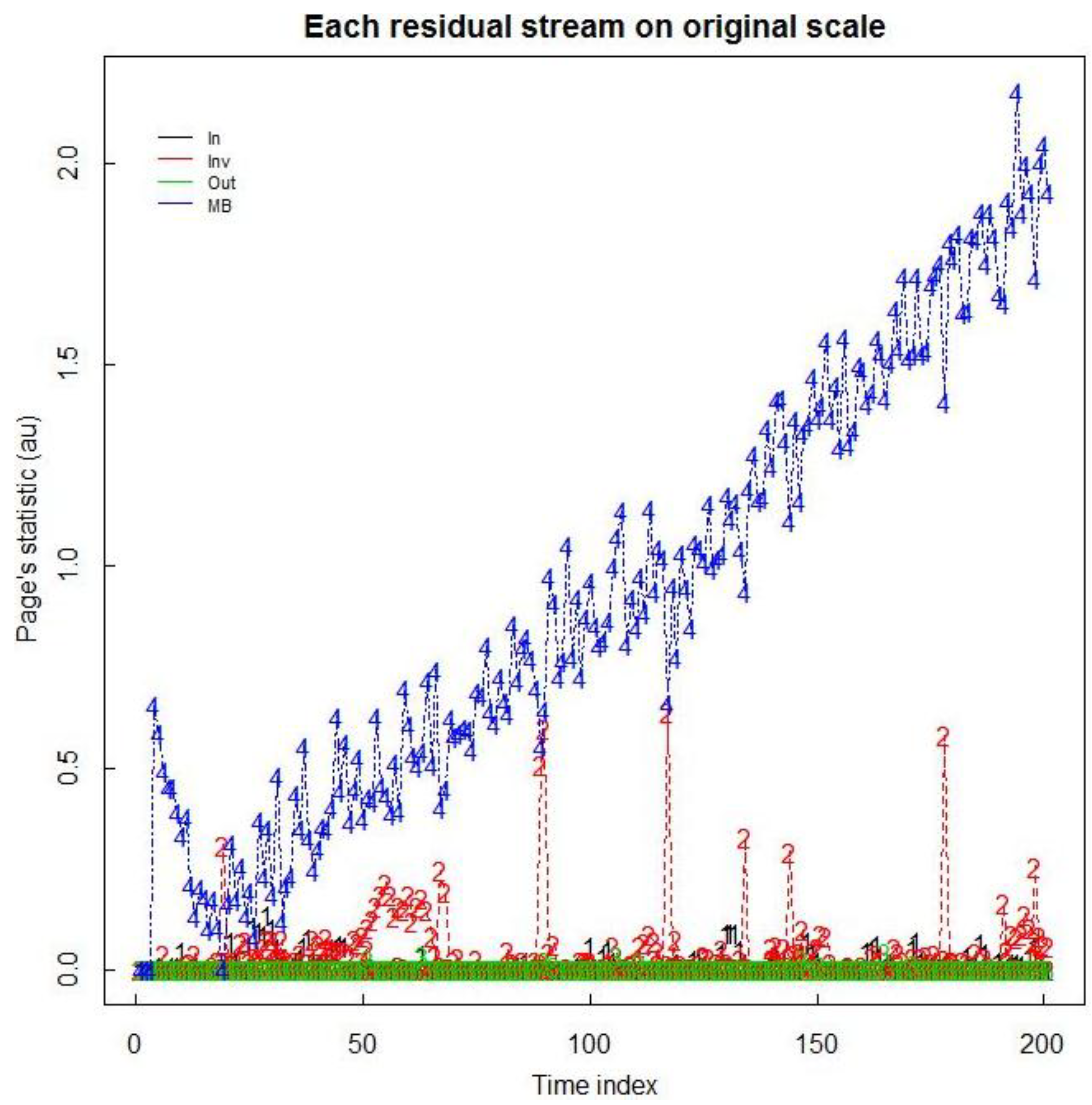
Figure 9 is Page’s cusum test applied to each of the residual streams in Figure 6. Page’s cusum test applied to a residual time series R t is given by S t = max ( 0 , S t 1 + R t k ) , where k is a control parameter. Page’s cusum test has close to the highest possible DP for many loss scenarios. Different tests will have the best DP for different loss scenarios, which partly explains why so many sequential tests have been proposed for NMA [23,26].
Figure 9. Page’s cusum test applied to each of the 14 (13 PM, one NMA) residual streams. To avoid cluttering the figure, only some residual streams are shown, as indicated.
Energies 08 00501 g009
Note 1: The cusum test C ( t ) = i = 1 t M B ( i ) which sums all MBs since the last period ignores individual transfers from tank 1 to tank 2 and has the highest DP among all possible tests for the equal-loss-per-balance-period case [1,23]. This means that evaluating each tank-to-tank transfer has lower DP than comparing the sum of tank 1 transfers to the sum of tank 2 transfers. Analogously, there is no free lunch regarding the use of SM and NMA data. That is, including SM data is an extension of NMA to include more sub-MBAs (each tank is a sub-MB area) and more frequent balance closures. Therefore, there are scenarios for which using NMA data alone leads to the highest DP. Such scenarios will involve widespread diversion over multiple tanks and time periods (unless such scenarios produce observables that could be monitored, which we are not considering here). The motives for evaluating SM data include resolving NMA alarm, detecting diversion to waste streams that should have relatively small amounts of Pu, and improving abrupt loss detection over more scenarios, meaning that there can be at least moderate DP for a wide range of diversion scenarios, which is not true for NMA data alone.
Note 2: In our context with a wide range of possible diversion scenarios, there cannot be a most powerful statistical test (a most powerful test is a test that has the highest DP for a specified scenario). Therefore, we cannot claim that using the average of the values of the individual maximum-over-the-BP Page’s cusum has higher DP than the alternative test that we evaluated that alarms if the maximum of the individual maximum Page’s cusum exceeds its threshold. We anticipate that ease of implementation and ease of estimating alarm thresholds for desired false alarm probabilities (FAPs) (such as 0.05 per year) will be important factors in choosing which hybrid option is preferred.
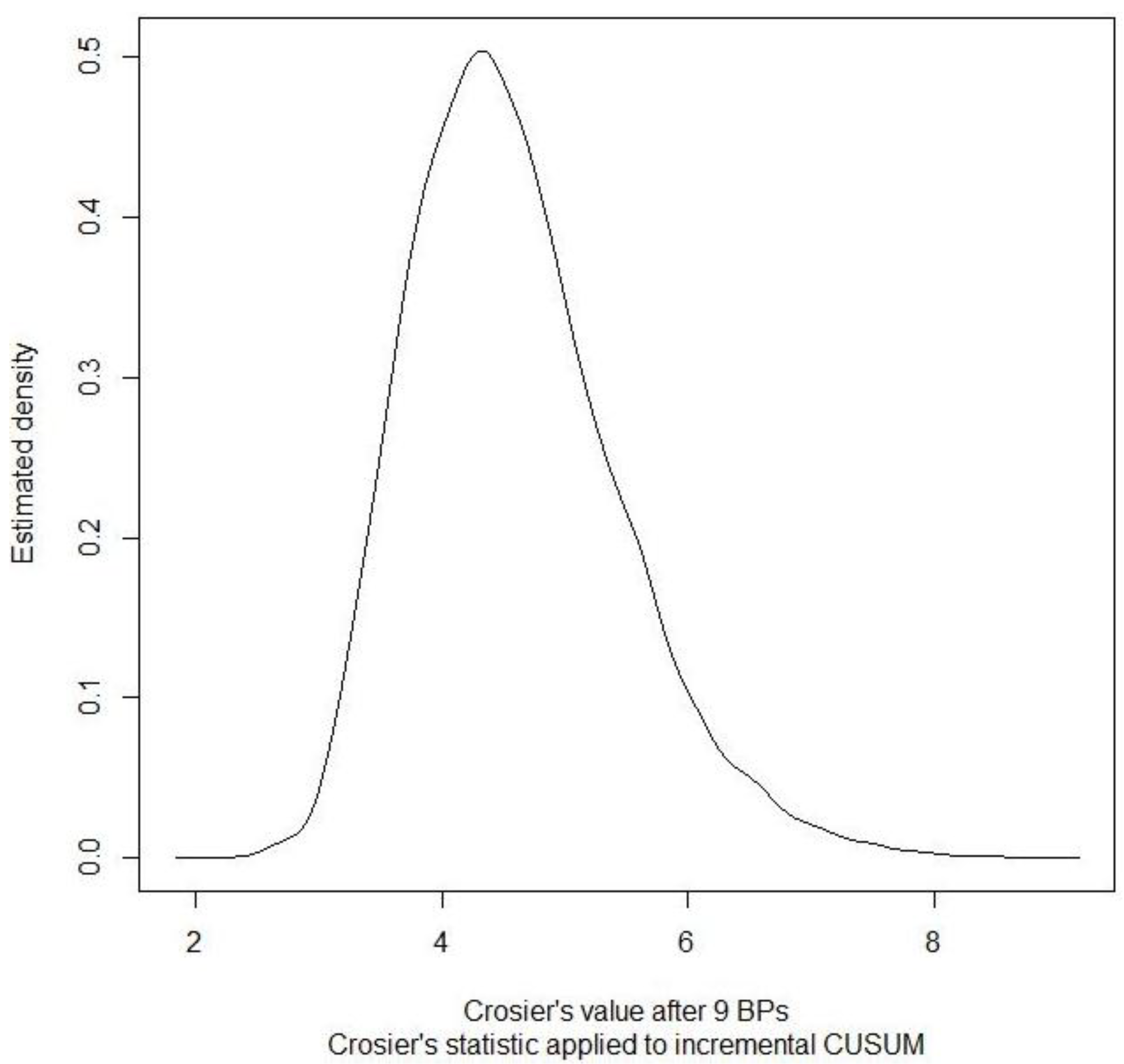
Figure 10 plots an example of the estimated probability density of Crosier’s statistic applied to incremental cusums in the 2-part hybrid described above at BP 9.
Figure 10. Example of the estimated probability density of Crosier’s statistic applied to incremental CUSUMs in the 2-part hybrid at BP 9. The data is simulated from the SPM of an electrochemical facility.
Energies 08 00501 g010
In general, we propose to estimate the DP of the safeguards system by estimating the system DP from PM combined with NMA using the following two steps (see Appendix 2):
a)
Describe diversion scenarios to inform how PM data should be evaluated to provide a means of event detection using expert elicitation if possible, and
b)
Evaluate P(alarm|diversion scenario), the conditional probability of an alarm for a given scenario. The alarm rule operates on p residuals r1, r2, …., rp which include MB values from NMA, plus residuals from monitoring “wait” and “transfer” modes in tank SM data. The probability P(alarm|diversion scenario) is a function of the true states of nature, the measurement system, and the alarm rule(s).
More specifically, we continue with the 13-vessel example to illustrate the two-part hybrid statistical test. It is straightforward to develop simulation-based estimates (see Figure 10) of alarm thresholds to maintain an overall 0.05 FAP per year following current convention with NMA data alone. However, because there are two tests in the hybrid test, there are two alarm thresholds, and one can allocate more of the 0.05 false alarm probability to one part of the hybrid or the other, using trial-and-error in simulation. For selecting alarm thresholds and comparing to standard time series such as sequences of independent and identically distributed (iid) normal random variables, it is convenient to transform each residual time series using the SITMUF-type transform (see Appendix A1); SITMUF stands for standardized independently transformed material unaccounted for. Upon doing so, we find that the alarm thresholds for the hybrid test consisting of the average value of the maximum of the Page’s cusums and Crosier’s cusum applied to incremental cusums are close to those for corresponding iid normal residuals. We do not expect exact agreement with independent normal residuals because the MB is strongly correlated with the other 13 residual streams.
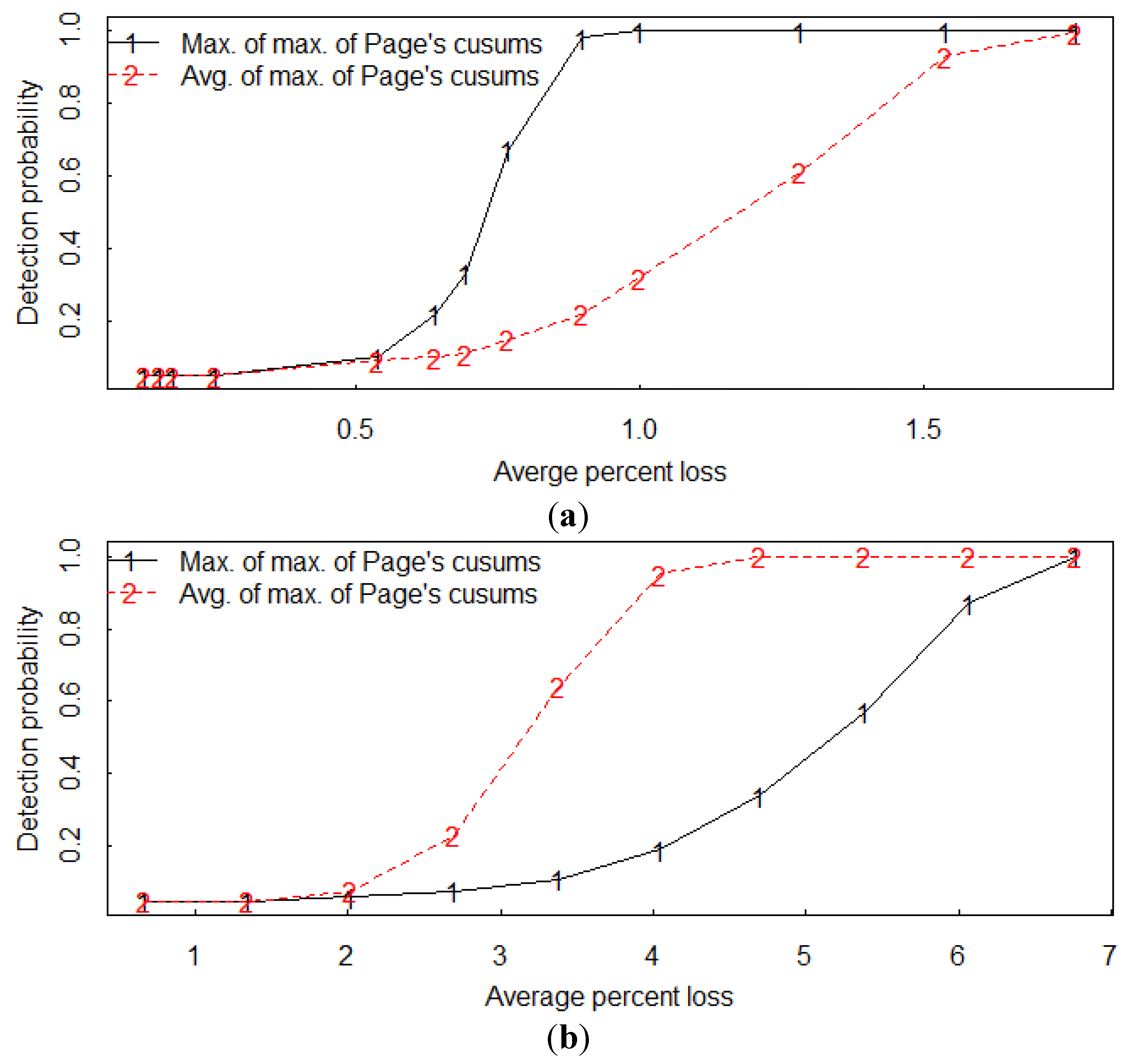
Having estimated the two alarm thresholds to achieve a 0.05 false alarm probability per operating year, we can easily inject various loss scenario effects in additional simulations to estimate system detection probabilities of the two-part hybrid statistical test. We have done simulations for both the average distance option applied to the maximum of the 14 individual Page’s cusums and also for using the maximum of the maximum of the 14 individual Page’s cusums. For example, Figure 11a is the estimated detection probability versus the average (over the 14 residual streams) one-day-abrupt loss from the input (the loss is expressed as an average of the total true amounts in each residual stream at a given time step) using the maximum of the maximum of the 14 Page’s cusums option and also using the average of the maximums. Figure 11b is the same as Figure 11a, but is for a wide-spread loss over all 13 residual streams. In Figure 11a,b, the loss occurred during one time step.
In Figure 11a, the maximum of the 14 maximum Page’s cusums has higher detection probability than the average of the 14 maximum Page’s cusums; this is expected because the loss occurred from only the single input residual stream. In Figure 11b, the opposite is true; again this is expected because the loss is spread over all 13 residual streams, so the average of the maximum of the 14 Page’s cusums has a relatively strong signal. The value of σMB is approximately 0.70 units each day, most of which arises from the large in-process inventory. The value of σ for the input residual is approximately 0.04. It makes sense to monitor residuals from any stream for which there is a predicted value and corresponding measured value; this example assumes there is a predicted value for all 13 residual streams, plus the MB stream (whose predicted value is, of course, zero).
Figure 11. Example estimated detection probabilities versus the average percent loss in a (a) local loss from the input and in a (b) non-local (widespread) loss from all 13 residual streams. The average is over all 13 residual streams during the one-time-step duration of the loss.
Energies 08 00501 g011

9. Conclusions and Summary

We described options to quantify the benefit of PM data by using P(alarm|diversion scenario) as the figure of merit, while using both PM and NMA residuals in the alarm rule. A key assumption is that the safeguards approach includes model-based predictions that can be compared to corresponding measurements, resulting in time series of residuals. The requirement for high-quality predictions leads to technical challenges in safeguarding either aqueous or electrochemical reprocessing facilities. For example, there is ongoing work aimed at high-quality modeling of the electrorefiner in an electrochemical facility [17]. Strictly speaking, our approach leads to high SNM loss detection probability only for the specified diversion routes; however, there is also high loss detection probability for any type of abrupt loss. See Appendix 2 for more detail. Also, in the context of international safeguards, there is not yet an approach to authenticate operator PM data; authentication will depend on facility type and is under investigation.
This paper introduced a hybrid alarm rule consisting of using the average distance computed from the maximum of the individual Page’s cusums and also using Crosier’s cusum applied to incremental cusums across balance periods. As a modification of (A), we also evaluated the performance of using the maximum of the maximum-over-the-BP values of each individual Page’s cusum (example results are given in Figure 11). A few other alarm rules have been evaluated in [1], all of which involve some type of pattern recognition applied to multivariate time series of PM and NMA residuals that arrive at equal or unequal frequencies in aqueous or electrochemical reprocessing facilities.
We believe it is acceptable to tune the pattern recognition to a list of important diversion scenarios to achieve high DP for those scenarios, provided P(alarm|diversion scenario) is non-zero for all scenarios so that the system is at least somewhat robust to any diversion scenario. Estimating P(alarm|diversion scenario) requires modeling and simulating the effects of each diversion scenario, so model uncertainty should be considered in future work. Model uncertainty has been considered in related safeguards contexts [32]. Section 8 provided an example; however, model uncertainty has not yet been included.

Acknowledgments

We acknowledge the US Department of Energy Material Protection, Control, and Accounting Program for funding this work.

Author Contributions

Tom Burr designed the study and conducted the simulations. Tom Burr, Michael S. Hamada, Larry Ticknor, and James Sprinkle wrote the manuscript

Appendix 1. Nuclear Material Accounting and Process Monitoring

A1.1. NMA

NMA has known limitations, particularly when large amounts of SNM are processed per unit time. Therefore, PM is increasingly important at large facilities [1,2,3,4,5,6,7,8,9,10,11,12,13,14,21]. Consider a facility having an input accountability tank (IAT), product accountability tank (PAT), and process operations between the IAT and PAT. If the true PAT output SNM is, for example, 8 kg less than the true IAT input SNM, then the desired safeguards conclusion is “alarm”. And, if SNM output is 8 kg less than SNM input, then various observables must be produced that could be measured. Therefore, PM attempts to verify that material flows and constituents are as declared by looking for the absence of such observables, such as changing material flow rates and constituents to misdirect the SNM to an undeclared exit stream. It is important to understand what types of facility misuse are possible and credible, and also to understand to what extent the various misuse scenarios can be detected.
To address known shortcomings of NMA, additional measures are taken. One additional measure is PM [1,2,3,4,5,6,7,8,9,10,11], which has recognized but currently unquantified benefits. PM includes analyzing the facility operator’s process control measurements to detect abnormal plant operation. Process control measurements are those used by the operator to control the chemical and/or physical processes. Example process control measurements in an aqueous reprocessing plant include (1) mass and density measurements in tanks; (2) inline flow meters; (3) concentration measurements of nonnuclear material reagents; and (4) process temperatures. Example process control measurements in an electrochemical reprocessing plant include (1) mass and density measurements in vessels; (2) voltages and current in the electrorefiner vessel; and (3) process temperatures. There are many roles for PM, and PM data have a variety of forms [1,2,3,4,5,6,7,8,9]. PM often involves more frequent but lower quality measurements than NMA [1,2,3,4,5,6,7,8,9,10,11]. While NMA estimates SNM mass balances and uncertainties, PM sometimes tracks SNM attributes qualitatively or in the case of solution monitoring, might track bulk mass and volume. PM data can also include very frequent high-dimensional spectral data from gamma detectors [20,21,22], or low-dimensional flow and/or in-tank volume data from flow meters or in-tank dip tubes. In some cases, PM data can be relatively high quality, such as in-line mass or volume flow measurements, and some current research is aimed at high-quality in-line SNM accountability measurements for electrochemical facilities [14,15,16,17,18,19] and aqueous facilities [7,8,20,21].
This article focuses on PM in which SNM inventories (bulk mass and/or Pu mass) in all vessels are measured frequently, such as every few minutes, or hour or day, and transfers are measured as they occur. If PM is simply more frequent balance closure (in the case that PM measures Pu mass for example) [23] showed that protracted loss detection is still very difficult; and, in fact, less frequent balance closure has higher loss detection probability for protracted loss. However, a model-based prediction for each SNM flow stream leads to time series of residuals that can be monitored for loss from any given stream. Therefore, there can be high loss detection probability for specified diversions from specified streams. But, an approach to combine PM and NMA is needed, so this article proposes a hybrid of period-driven and data-driven hypothesis testing.
Unique statistical challenges in combining NMA and PM residual time series include: PM and NMA data are often collected at different frequencies; PM residual times often have a probability distribution that cannot be adequately modeled by a Gaussian distribution, not all PM and NMA data streams are independent, and the monitoring scheme must have reasonably high detection probability for both abrupt and protracted diversion. This article considers the situation in which the PM residuals are generated on the same fixed time schedule as are NMA residuals, so all residuals will arrive at the same frequency, and the situation in which tank events are marked as they occur, so the PM residuals do not all arrive at the same frequency [1,2,3,4,5,6].
In NMA, a sequence of MBs can be evaluated over a fixed period (“period-driven”), or not (“data-driven”), and in either case, the covariance matrix of a sequence of MBs, ∑MB, is estimated. In data-driven evaluation, some type of sequential testing is used, usually including the basic two tests: MUF (material unaccounted for, which is the same as the MB, which is good to monitor to detect a one-time abrupt loss) and CUMUF (cumulative MUF, which is good for detecting longer-term loss). Another good choice is Page’s cusm (i.e., cumulative sum), which is defined at period t as Pt = maximum (Pt−1 + SITMUFtk, 0), where SITMUF is the standardized, independently transformed MUF (should have zero mean, unit variance, and be uncorrelated with all previous SITMUF values), k is a control parameter usually defined to be 0.5 [12].
One issue in sequential testing is that the test should have good alarm probability for either abrupt or various types of protracted diversion. The best sequential test depends on the type of loss so no test can be uniformly more powerful for all loss types. The CUMUF test is good if diversion begins on the first balance period and continues at the same rate for all subsequent periods. Page’s cusum test is optimal if the diversion begins in an arbitrary period, persists at the same level for an arbitrary period, and then returns to zero. Slight complications arise due to the transformation required (that uses ∑MB) to convert a MUF sequence into a SITMUF sequence, but Page’s cusum test applied to the SITMUF sequence is among the most versatile tests, and is arguably the most versatile [1,10,12].
Advantages of frequent NMA include: (a) improved abrupt loss alarm probability; (b) timeliness; (c) improved alarm/anomaly resolution; and (d) refinement of measurement error models [1,3,24]. Regarding measurement error models, metrology for nuclear safeguards includes the notion of random and systematic errors as in the international target values for uncertainty [24]. For example, a measured quantity M is assumed to vary around the corresponding true quantity T, with M = T + R + S, where R is random error and S is systematic error, and the standard deviation of RR) and the standard deviation of SS) are estimated using well-characterized standards. Straight-forward variance propagation is then used to estimate ∑MB [12].
Regarding SNM in-process inventory that is difficult to measure (called holdup), if there were no measurement error in the transfers and inventory, then the MB would equal the change in holdup plus the true loss [25]. The presence of measurement error complicates MB evaluation, and the presence of non-negligible holdup together with measurement error further complicates MB evaluation. Nevertheless, provided σMB is well estimated (not a scientific challenge, but often an engineering challenge constrained by limited time and budget), it is understood that the magnitude of σMB can be used to easily estimate the loss detection capability if one assumes that the MB is approximately normally distributed. We end this sub-section with three summary remarks regarding NMA:
Remark 1: NMA involves periodically measuring facility inputs, outputs, and inventory to compute an MB. Sequences of MBs are analyzed using a sequential test such as Page’s cusum test. Assume that an aqueous facility has a measurement error standard deviation of σMB = 0.3% of throughput (a reasonably small percentage assuming international target values of measurement performance [24]). Then, assuming the measured MB has approximately a Gaussian distribution around the true MB, and international safeguards detection goals (95% detection probability and 5% false alarm probability) the diversion would have to equal 3.3 × 24 kg = 92 kg for an 8000 kg Pu per year facility. This 92 kg is much larger than one significant quantity (SQ), which is 8 kg for Plutonium [1,6,8,9]. Therefore, safeguards goals are not likely to be met in large throughput facilties through NMA alone.
Remark 2: Regarding holdup, if there were no measurement error in the transfers and inventory, then the expected value of the MB would equal the change in holdup plus the true loss L. The presence of measurement error complicates MB evaluation, and the presence of non-negligible holdup together with measurement error further complicates MB evaluation. Nevertheless, provided σMB is well estimated, which is often an engineering challenge constrained by limited time and budget, and which often invokes modeling and simulation to estimate holdup and model measurement processes, it is understood [1,12,23,26] what σMB and/or ∑MB implies about loss detection capability.
Remark 3: Facilities that cannot meet the detection probability (DP) goals have negotiated-levels of “additional measures”. For example, the Rokkasho reprocessing facility (RRP) in Japan will include PM as a separate, additional safeguards measure.

A1.2. Process Monitoring (PM)

PM often enables a type of frequent NMA, which is usually referred to as near real time accounting (NRTA). NRTA is typically described as: frequent balance closures based mostly on measurements of the shipments and receipts, with varying capability to measure or estimate in-process inventory. In practice, “frequent” is typically daily or weekly (however, PM-based balance closures are common on a per-batch basis which could be daily or multiple times per day). Facilities that close balances very frequently, such as daily or after each batch transfer, rely on various shortcuts or partial measurements. For example, it is rare to equip each processing unit with in-line holdup or in-process inventory monitors. Therefore, either engineering estimates, or historical by-difference estimates are used for negotiated portions of the in-process inventory measurements [25]. In the NRTA scheme at the THORP (“thermal oxide reprocessing plant”) in England [26], full material balance closures are not as often as weekly because of the infrequency of Pu concentration measurements. Full balance closures are less often than weekly, but pseudo-balance closures using empirical relations to estimate the Pu concentration are quite frequent (roughly daily). Although in-line dip tubes measure vessel volume every few seconds, there might not be a capability to measure the Pu concentration in-line. In-line dip tubes estimate solution density, so empirical relations together with the density estimate can infer (but not directly measure) the Pu concentration [27]. An NRTA system that measures all material is preferred, but even the best system will typically rely on partial measurements and/or engineering estimates for at least part of the in-process material [1,7,25].
Solution monitoring (SM) is a type of PM. Consider level (L), density (D), and temperature (T) measurements of solution in a reprocessing facility. Unless there is an in-line Pu concentration measurement, then empirical relations linking Pu concentration to D and T for a given nitric acid concentration are required to estimate the Pu concentration. Together with a volume estimate using the calibrated V = f (L) + error relation, an estimate of Pu mass is available. This is a pseudo-measurement because unless Pu is actually measured, we cannot be sure that Pu has not been diverted in some manner without reducing solution volumes. The use of such pseudo-measurements or pseudo-balance closures means that most examples of NRTA and PM are not, strictly speaking, full NMA. And, even if full NMA were done frequently, such as daily, then [23] showed that protracted diversion is still not detected with high probability. In fact, less frequent NMA has a higher detection probability than frequent NMA for protracted diversion that occurs over a long time period. However, PM can have a high detection probability for specified diversions for which it is tuned, while having only a slightly lower detection probability than infrequent NMA for wide spread diversion over time and/or space.
The type of PM just described is essentially a poor-man’s NRTA and can lead to high DPs for abrupt diversion. Reference [27] showed that SNM loss during tank “wait modes” would be much easier to detect than SNM loss during “transfer modes” (see Section 3). This is largely due to canceling systematic errors when two level measurements in the same tank are compared. If we need high confidence in PM only during transfer modes, this is a potential savings. However, because there is no in-line Pu concentration measurement, the caveats mentioned above are in effect. The adversary could divert without an alarm during a wait mode by replacing the removed volume with the correct density solution. If this occurred over a one day period (the daily Pu throughput is approximately 50 kg), then downstream Pu concentrations could be back at expected values by the next monthly balance closure when Pu concentrations are measured in all key tanks. We end this sub-section with three summary remarks regarding PM:
Remark 4: Short-cut assay methods such as a volume and a calculated SNM concentration do not directly measure the SNM of interest but are often used for some of the measurements in frequent NMA (such as every 10 days). PM directly supports NMA if PM is used to estimate holdup [1,28,29].
Remark 5: PM directly supports NMA if PM is used to estimate holdup [1,28,29].
Remark 6: Currently, there is no attempt to quantitatively use PM to meet DP goals.

Appendix 2. Data Fusion: Period-Driven and Data-Driven Pattern Recognition

A2.1. Data Fusion

In NMA, diversion detection probability (DP) is the safeguard’s system main figure of merit for a specified diversion amount and time frame. Because σMB determines the DP [12], via the assumed Gaussian distribution of the MB, efforts are continually made to reduce σMB. In combining PM data with NMA data, we propose to retain diversion DP as the figure of merit, but extend the diversion scenario description from SNM amount and time frame to include how the SNM is diverted. A key task is then to estimate the probability distribution of the combined PM and NMA residuals in the no-diversion case and in the diversion case. The residual probability distribution in the no-diversion case can be estimated by analysis of real facility data, and in the diversion case can be estimated by modeling and simulating the effects of facility misuse on real data [1,22].
Once the probability distributions are estimated in the no-diversion and diversion cases for the combined NMA and PM residuals [1,2,5,6], data fusion to combine NMA and PM residuals can be done at the feature, score, or decision levels to reach an overall decision [1]. The feature level is the raw data, which is rarely effective. The score level is some transform of the raw data, such as a computed residual. The decision level is a binary-valued “pass” or “fail” at the level of the individual residual stream. Converting each residual stream to a binary-valued pass or fail is simple, but loses information. Here, we perform data fusion at the score level, where the score is the NMA or PM residual.
We propose to estimate the DP of the safeguards system by estimating the system DP from PM combined with NMA using the following two steps:
a)
Describe diversion scenarios to inform how data should be evaluated to provide a means of event detection using expert elicitation if possible, and
b)
Evaluate P(alarm|diversion scenario), the conditional probability of an alarm for a given scenario. The alarm rule operates on p residuals r1, r2, …., rp which include MB values from NMA, plus residuals from monitoring “wait” and “transfer” modes in tank SM data. The probability P(alarm|diversion scenario) is a function of the true states of nature, the measurement system, and the alarm rule(s). Depending on the desired alarm rule, some subset of r1, r2, …., rp could perhaps be dichotomized into “exceeds threshold” (1-valued) or “does not exceed threshold” (0-valued).
Each diversion path has signatures (observables), so including relevant PM measurements with NMA data can enable pattern recognition approaches. See Section 4 for an example involving diversion to the waste hull in the head-end. For a given scenario, P (alarm at any time 1, 2, …, t|diversion scenario) can be estimated using simulated effects superimposed on real or simulated background data for any SM approach. Lyman [33] points out that not all diversion scenarios can be anticipated, and we agree. However, P(alarm at any time 1, 2, …, t|diversion scenario) can be estimated for the scenarios thought to be most credible, and although P(alarm at any time 1, 2, …, t|diversion scenario) cannot be estimated for unspecified scenarios, statistical tests can be used that have some signal to detect any shift in a probability distribution, so we claim at least that P(alarm at any time 1, 2, …, t|diversion scenario) is higher than the false alarm rate for any credible but unspecified scenario.
Specific residuals r1, r2, …., rp are used from NMA and PM in the two examples in Section 8. In fusing NMA and PM data, NMA uses Page’s cusum test to detect trends over time [1,12,23,26]. One could also use Page’s cusum test to define residuals that can detect trends over multiple wait and/or transfer modes for a given tank or pair of tanks.

A2.2. Hybrid of Period-Driven and Data-Driven Pattern Recognition

A2.2.1. Period Driven Hypothesis Testing

Suppose NMA and PM residuals are evaluated frequently (such as every day or every 10 days), but a statistical decision is made every year, to alarm or not. Yearly decisions are practical in safeguards because facilities often schedule a partial shutdown and clean out of the facility, which provides a convenient time to have most SNM in relatively easy-to-measure forms.
One goal for international safeguards using period-driven testing with a one-year decision period is to detect a loss of a significant quantity (SQ) with probability 0.95 with a 0.05 false alarm probability (FAP) per year, testing for loss only, not for gain, so one-sided statistical hypothesis testing is used. Assuming the MB is approximately Gaussian distributed, one can achieve a 0.95 DP to detect a diversion of 3.3 σMB using period-driven NMA with yearly balance closure (non-sequential testing), where the alarm threshold of 1.65 σMB corresponds to a 0.05 FAP. However, suppose the adversary diverts ½ of the desired material over months 7 to 18, straddling two balance periods (year one and year two). For the system to fail, the system must fail to detect the diversion of 1.65 σMB in year one, and fail to detect the diversion of 1.65 σMB in year two, which occurs with probability 0.5 × 0.5 = 0.25, so the DP is reduced from 0.95 to 1 − 0.25 = 0.75 [1]. Addressing the adequacy of the Gaussian approximation in the context of MB evaluation is beyond our scope here; however, in many cases, the MB is computed from sums and differences of many measurements, so the central limit theorems strongly suggest that the Gaussian approximation is reasonable.

A2.2.2. Data-Driven Hypothesis Testing

To mitigate a decrease in DP (for example, from 0.95 to 0.75 in Section A2.2.1) arising from the adversary diverting across two balance periods, one can instead use a sequential (data-driven) test that has no fixed period at which decisions are made. Instead, the test continues until a decision to alarm or not is made, and then starts over. We can design a sequential test to have a long average run length (ARL) between false alarms, such as 20 years, which corresponds to the 0.05 per-year FAP assumed in the previous paragraph.
One effective sequential test is Page’s cusum test defined at period t as Pt = maximum (0, Pt−1 + ytk), where yt is the SITMUF sequence and k is a user-chosen control parameter that is optimal for detecting a shift from mean 0 to mean 2k at an arbitrary period. Page’s cusum test applied to an independent and identically distributed sequence of N(0,1) random variables (such as the SITMUF sequence) has a DP of approximately 0.79 for this total loss of 3.3 σMB spread evenly over months 7 to 18 (across balance periods 1 and 2 in period-driven testing) if the ARL is approximately 20 years and k = 0.5. And, if the loss is on any one balance period, the DP using Page’s cusum test is approximately 0.99 (on the basis of 104 simulations in R, ensuring approximately a 20-year ARL between false alarms), but is 0.95 for the period-driven yearly balance. If there is a total loss of 1.65 σMB on a single balance period during year one, then the period-driven yearly balance DP is only 0.50, while the DP using Page’s cusum test is approximately 0.96, again with a 20-year ARL. There is no avoiding the fact that protracted diversion has lower DP than abrupt diversion, but Page’s cusum test manages to retain high DP for abrupt loss while having reasonable DP for protracted loss.

A2.2.3. Hybrid of Period-Driven and Data-Driven Testing

As shown in Section A2.2.1, period-driven testing does not have good DP if the adversary diverts modest amounts of SNM over multiple decision periods. Therefore, if period-driven testing is used, we advocate in addition, data-driven monitoring of a scalar or vector-valued residual from each period. A scalar residual could be monitored over multiple periods using Page’s cusum as described, for example, over multiple 30-day periods.
To illustrate using NMA alone, consider using a hybrid test consisting of a data-driven Page’s cusum together with an annual period-driven cusum. For a total loss of 3.3 σMB spread evenly over months 7 to 18 (across balance periods 1 and 2 in period-driven testing), we used 105 simulations to estimate a DP of the hybrid test of 0.88 (the DP depends on the alarm thresholds, so this is one example DP with alarm thresholds chosen arbitrarily, except that we must achieve an FAP of 0.05 per year). The hybrid-test’s DP of 0.88 is higher than the 0.79 DP for Page’s cusum alone (Section A2.2.2), and slightly lower than using a data-driven Page’s cusum alone (0.89). Note that for many choices of the two alarm thresholds (one chosen threshold for the data-driven Page’s cusum and one for the annual period-driven cusum), if the true loss occurred like clockwork, from months 1 to 12 or from months 13 to 24, for example, then the hybrid-test’s DP would be higher than that of a data-driven Page’s cusum. Also, as an aside, another option for a hybrid of period-driven and data-driven testing is to simply restart Page’s cusum test at the start of every new year and decide to alarm on not at the end of the previous year. This is a type of truncated Page’s cusum test that is also vulnerable to loss patterns that occur over multiple year periods. For completeness, we also note here that a monitoring option known as the scan statistic has the highest DP (0.95 in this case, verified by simulation) if one knows that a loss will occur over a 12-month period with an unknown start period (such as month 7). In this context, the scan statistic computes a moving sum of months 1 to 12, 2 to 13, 3 to 14, etc. The scan statistic is not used in safeguards to our knowledge, but is widely used in other applications, for example, to detect regions of residuals having the same sign. Of course in practice one would not know the loss duration, so a variable-length scan statistic would be used. However, in practice, one also would not know that the loss would occur continuously over multiple periods, so the scan statistic is not as compelling at Page’s cusum when one considers the myriad of possible loss patterns. So, one effective hybrid test is the combination of Page’s ongoing cusum and annual period-driven cusums just described.
Next, we consider monitoring both NMA and PM residuals. The PM residuals can be generated by option 1 (generated every hour for example, by monitoring flow rates), or by option 2 (generated as events occur using event marking). Both option 1 and option 2 residuals will in general be generated at different time steps for different areas of the facility.
One monitoring option is to compute Page’s cusum and a periodic cusum for each residual stream. Because of complicated dependencies among some of the residual streams, we recommend simulation to choose alarm thresholds for this hybrid test. Another monitoring option is to monitor multivariate residuals by using a multivariate sequential test, such as Crosier’s cusum [3], which is a multivariate version of Page’s cusum defined as follows. First define a scalar C t = { ( S t 1 + R t ) T Σ 1 ( S t 1 + R t ) } ( 1 / 2 ) , where S t = S t 1 + R t k  if  C t > k and S t = 0 if C t k , and the vector k is defined as k = ( S t 1 + R t ) k / C t , with the scalar k being a specified control parameter and R t being the residual vector. Because k is in the same direction as ( S t 1 + R t ) , the use of S t = S t 1 + R t k shrinks the cumulative sum vector S t toward 0. To explicitly view the shrinkage toward 0, note that S t = ( S t 1 + R t ) ( 1 k / C t ) . Upon calculation of S t , a scalar Y t is calculated, defined as Y t = ( S t T Σ 1 S t ) ( 1 / 2 ) , and the test alarms if Y t exceeds a threshold h. As does the univariate Page’s cusum, Crosier’s multivariate cusum requires a scalar control parameter k and a threshold h [1].
One approach to deal with the fact that the PM residuals are generated at different time steps is to convert all residual streams to the frequency of the most frequently recorded residual stream, simply by repeating the value of the most recent residual. Another approach is to aggregate the more-frequently recorded residual streams to the frequency of the slowest-frequency stream. Periodic data-driven cusums of each residual streams would be monitored in conjuction with Crosiers’ cusum.
To summarize this section, to monitor the multiple time series of PM and NMA residuals, we propose a hybrid testing scheme that includes both period-driven and data-driven hypothesis testing. One of the simplest options is to compute Page’s cusum and a periodic cusum for each residual stream. Because of complicated dependencies among some of the residual streams, we use simulation to choose alarm thresholds for this hybrid test and to estimate the system DP.

A2.3. Pattern Recognition

In a typical pattern recognition problem, the data consist of n cases of (y, X) pairs where the integer y ϵ (1, 2,..., J) is the class and X is a p-dimensional predictor vector. The goal is to use X to predict the class y, and this task is sometimes called classification, discriminant analysis (DA), or supervised learning. Regarding notation, vectors and scalars can be distinguished by context and definition. For example, y is a scalar and X is a p-dimensional vector.
There are many approaches to pattern recognition. Some attempt to estimate the probability density of the predictor vector, X, given its class (i.e., the class conditional probability, P(X|y)) by assuming some convenient distribution for X|y such as multivariate Gaussian which linear discriminant analysis (LDA) assumes [1]. Other methods of estimating densities assume only that the distribution is stationary over time. Such methods are typically called non-parametric or distribution-free methods [1,34]. Space does not permit a review of all pattern recognition options.
Alternative strategies attempt to estimate Bayes rule without estimating the class conditional probabilities, such as support vector machines (SVMs), which construct nonlinear decision boundaries for the classes in a manner similar to flexible discriminant analysis (FDA). Hastie et al. [35] describe SVMs, FDA, and also describe nearest neighbor classifiers and learning vector quantization.
The most common pattern recognition data model assumes that a categorical response y depends on a fixed-dimension predictor X. The pattern recognition task is to estimate f(X) = Prob(y = 1| X). The most well studied version of this task assumes: (1) all components of X are real-valued; (2) X has fixed dimension; and (3) training cases consisting of (y, X) pairs are independent.

A2.3.1. Pattern Recognition for NMA and PM Data

Currently, most safeguards conclusions are made at the end of a NMA balance period, but the increasing role of PM is driving a change to make data-driven conclusions. As an example, consider a 4-tank balance area consisting of a buffer tank 1 which ships in batch mode to a feed tank 2 which continuously feeds a “black box” area where chemical processing occurs. The black box ships continuously to a receipt tank 3, which ships in batch mode to a buffer tank 4. For process control reasons, the plant operator periodically samples tanks 1 and 4 to measure the SNM concentration and uses mixing rules and measured flow rates to estimate the Pu concentration and mass in tanks 2 and 3. Online measurements of tank level (which is calibrated to volume), density, and temperature are available every few seconds, so tank volume V and mass M (mass = volume × density) are available every few seconds from each tank. These (V, M) measurements are PM measurements. NMA computes the MB as estimated Pu into tank 1 minus the estimated Pu out of tank 3. There are also neutron detectors in the black box area to monitor Pu inventory in an indirect semi-quantitative manner.
The pattern recognition tasks for this example are: (1) to recognize any departure from normal process operations; and (2) to recognize specific misuse scenarios that are judged to be credible. Some of the technical challenges are:
  • For (1), anomaly detection as a special case of pattern recognition has been approached using density estimation [36];
  • For (2), signatures and patterns of specific misuse scenarios are usually modeled and there is consider model uncertainty, so the probability density function (pdf) of each misuse scenario is uncertain (this source of uncertainty is currently ignored);
  • PM measurements overlap with NMA measurements (example: the same instrument that measures tank V for NMA is used for PM) so there are between-data-type correlations;
  • PM and NMA data are on differing time scales, and
  • PM data captures many innocent sources of process variation.
The main task for pattern recognition is to combine residuals from NMA and PM to provide data-driven pattern recognition (operating as declared or some type of misuse), period-driven (at the end of each day or balance period, make a statistical decision to alarm or not) pattern recognition, and some type of hybrid of period- and data-driven pattern recognition as discussed in A.
Remark 7: All predictors for pattern recognition will be based on model fitting and associated residuals. As in “phase 1” control charting [37] for production processes, the pdf of the time series of a vector of residuals can be estimated. However, estimation of the residual vector’s pdf requires a combination of modeling and data analysis as illustrated by example in [1]. The approach in [1] does not distinguish sensor faults from SNM loss, but assuming no more than one sensor malfunctions within small time windows, Howell et al. [38] and Hines et al. [39] illustrate options that are also based on monitoring residuals, using regression and other statistical tools that were first applied to monitor sensor health for the U.S. Nuclear Regulatory Commission. As far as the authors are aware, only Howell et al. [38] have attempted to distinguish sensor faults from SNM loss.
Recall that in NMA alone, the figure of merit is P(alarm|L, time period) where L is the SNM loss (due to diversion or innocent loss). And, the central limit theorem effect operating on the many measurements comprising an MB leads to the MB having approximately a Gaussian distribution, so P(alarm|L, time period) for a given alarm threshold is a function only of σMB. In period driven testing, the time period is fixed in advance, such as one year, and [23] showed that in the Gaussian case, a single CUMUF test at the end of each time period has the highest DP for the worst-case diversion. And, the worst-case diversion vector L is proportional to the row sums of ∑MB. In data-driven (sequential) testing, the time period must be specified for each diversion of interest in order to estimate P(alarm|L, time period), and more complicated alarm rules than the CUMUF rule must be used, such as Page’s cusum. PM residuals will not always be adequately modeled using a Gaussian distribution. For example, some event-marking-based PM data such as tank-to-tank transfer differences (see Section 3) have a multi-modal distribution. Such non-Gaussian behavior complicates the pattern recognition task. In addition, with time series of combined PM and NMA residuals, either hybrid or pure data-driven testing will be used in the context of evaluating P(alarm|L, time period), where how the diversion occurs must also be specified.

Conflicts of Interest

The authors declare no conflict of interest.

References

  1. Burr, T.; Hamada, M.S.; Skurikhin, M.; Weaver, B. Pattern recognition options to combine process monitoring and material accounting data in nuclear safeguards. Stat. Res. Lett. 2012, 1, 6–31. [Google Scholar]
  2. Burr, T.; Hamada, M.S.; Ticknor, L.; Weaver, B. Model selection and change detection for a time-varying mean in process monitoring. Nucl. Instrum. Methods Phys. Res. A 2014, 751, 79–87. [Google Scholar] [CrossRef]
  3. Burr, T.; Bakel, A.; Bryan, S.; Budlong-Sylvester, K.; Damico, J.; Demuth, S.; Ehinger, M.; Garcia, H.; Howell, J.; Johnson, S.; et al. Roles for process monitoring in nuclear safeguards at aqueous reprocessing plants. J. Nucl. Mater. Manag. 2012, 40, 42–53. [Google Scholar]
  4. Burr, T.; Suzuki, M.; Howell, J.; Hamada, M. Loss detection results on simulated tank data modified by realistic effects. J. Nucl. Sci. Technol. 2012, 49, 209–221. [Google Scholar] [CrossRef]
  5. Burr, T.; Suzuki, M.; Howell, J.; Hamada, M.; Longo, C. Signal estimation and change detection in tank data for nuclear safeguards. Nucl. Instrum. Methods Phys. Res. A 2011, 640, 200–221. [Google Scholar] [CrossRef]
  6. Suzuki, M.; Hori, J.; Nagaoka, S.; Kimura, T. Study on loss detection algorithms using tank monitoring data. J. Nucl. Sci. Technol. 2009, 46, 184–192. [Google Scholar] [CrossRef]
  7. Ehinger, M.; Chesnay, B.; Creusot, C.; Damico, J.; Johnson, S.; Weuster, J.; Masuda, S.; Kajii, M. Solution monitoring applications for the Rokkasho reprocessing plant. In Proceedings of the 7th International Conference on Facilities Operations: Safeguards Interface, Charleston, SC, USA, 29 February–5 March 2004.
  8. Spent Fuel Reprocessing Options. Available online: http://www-pub.iaea.org/MTCD/publications/PDF/te_1587_web.pdf (accessed on 10 November 2014).
  9. Ehinger, M.; Zack, N.; Hakkila, A.; Franssen, F. Use of Process Monitoring for Verifying Facility Design for Large-Scale Reprocessing Plants; Los Alamos National Laboratory Technical Report LA-12149-MS, Oak Ridge National Laboratory Technical Report ORNL 11856; Oak Ridge National Laboratory: Oak Ridge, TN, USA, 1991. [Google Scholar]
  10. Burr, T.; Hamada, M.S. Bayesian updating of material balances covariance matrices using training data. Int. J. Progn. Health Monit. 2014, 5, 1–13. [Google Scholar]
  11. Burr, T.; Hamada, M.S. Smoothing and time series modeling of nuclear material accounting data for protracted diversion detection. Nucl. Sci. Eng. 2014, 177, 307–320. [Google Scholar] [CrossRef]
  12. Burr, T.; Hamada, M.S. Revisiting statistical aspects of nuclear material accounting. Sci. Technol. Nucl. Install. 2013. [Google Scholar] [CrossRef]
  13. Burr, T.; Skurikhin, M. Proliferation Evaluation Criteria in Next-Generation Reprocessing Options: Combining Process Monitoring With Nuclear Material Accounting for Improved Safeguards; Los Alamos National Laboratory Technical Report 2012 LA-UR-12-22504; Los Alamos National Laboratory: Los Alamos, NM, USA, 2012. [Google Scholar]
  14. Cipiti, B.; Duran, F.; Key, B.; Liu, Y.; Lozano, I.; Ward, R. Modeling and Design of Integrated Safeguards and Security for in Electrochemical Reprocessing Facility; SAND2012-9303; Sandia National Laboratory: Albuquerque, NM, USA, 2012. [Google Scholar]
  15. Bae, J.; Nam, H.; Yi, K.; Park, B.; Hwang, S. Numerical assessment of pyrochemical process performance for PEACER system. Nucl. Eng. Des. 2010, 240, 1679–1687. [Google Scholar] [CrossRef]
  16. Fukushima, M.; Nagai, T.; Kofuji, H.; Hirano, H.; Myochin, M. Development of measurement techniques for density and liquid level of molten salt to assess an inventory in equipment of pyro-processing. In Proceedings of the 51st Annual Meeting Institute of Nuclear Materials Management, Baltimore, MD, USA, 11–15 July 2010.
  17. Zhang, J. Kinetic model for electrorefining, part I: Model development and validation. Prog. Nucl. Energy 2014, 70, 279–286. [Google Scholar] [CrossRef]
  18. Vaden, D. Fuel conditioning facility electrorefiner process model. Sep. Sci. Technol. 2006, 41, 1985–2001. [Google Scholar] [CrossRef]
  19. Vaden, D. Fuel conditioning facility electrorefiner model predictions versus measurements. In Proceedings of the INL/CON-07-12980 15th Symposium on Separation Science and Technology for Energy Applications, Gatlinburg, TN, USA, 21–25 October 2007.
  20. Orton, C.; Fraga, C.; Christensen, R.; Schwantes, J. Proof of concept experiments of the multi-isotope process monitor: An online, nondestructive, near-real-time monitor of spent nuclear fuel reprocessing facilities. Nucl. Instrum. Methods Phys. Res. A 2011, 672, 38–45. [Google Scholar] [CrossRef]
  21. Casella, A.; Peterson, J.; Jordan, E.; Verdugo, D.; Skomurski, F.; Lines, A.; Bryan, S.; Levitskaia, T. On-line monitoring for control and safeguarding of radiochemical streams at spent fuel reprocessing plants. In Proceedings of the 52nd meeting Institute of Nuclear Material Management, Palm Desert, CA, USA, 17–21 July 2011.
  22. Garcia, H.; Burr, T.; Coles, G.; Edmunds, T.; Garrett, A.; Gorensek, M.; Hamm, L.; Krebs, J.; Kress, R.; Lambertia, V.; et al. Integration of facility modeling capabilities for nuclear nonproliferation analysis. Prog. Nucl. Energy 2011, 54, 96–111. [Google Scholar] [CrossRef]
  23. Avenhaus, R.; Jaech, J. On subdividing material balances in time and/or space. J. Nucl. Mater. Manag. 1981, 10, 24–33. [Google Scholar]
  24. Zhao, K.; Penkin, M.; Norman, C.; Balsley, S.; Mayer, K.; Peerani, P.; Pietri, C.; Tapodi, S.; Tsutaki, Y.; Boella, M.; Renha, G.; Kuhn, E. International Target Values for Uncertainty Components in Fissile Isotope and Element Accountancy for the Effective Safeguarding of Nuclear Materials; Safeguards Technical Report 368; International Atomic Energy Agency (IAEA): Vienna, Austria, 2010. [Google Scholar]
  25. Yamaya, K.; Nobuharu, S.; Iseki, T.; Kawai, A.; Iwamoto, T. Plutonium inventory estimation of extraction cycles at Rokkasho reprocessing plant. In Proceedings 50th Annual Meeting Institute Nuclear Materials Management, Phoenix, AZ, USA, 12–16 July 2009.
  26. Jones, B. Near real time materials accountancy using SITMUF and a joint page’s test: Improvement of the test. ESARDA Bull. 1989, 16, 13–19. [Google Scholar]
  27. Burr, T.; Coulter, A.; Howell, J.; Wangen, L. Solution monitoring: Quantitative and qualitative benefits to safeguards. J. Nucl. Sci. Technol. 2003, 40, 256–263. [Google Scholar] [CrossRef]
  28. Beyerlein, A.; Geldard, J.; Weh, R.; Eiben, K.; Dander, T. Experimental Validation of Pulsed Column Inventory Estimators; Los Alamos National Laboratory Technical Report LA-UR-91-2872; Los Alamos National Laboratory: Los Alamos, NM, USA, 1991. [Google Scholar]
  29. Candy, J.; Rozsa, R. Safeguards design for a plutonium concentrator—An applied estimation approach. Automatica 1980, 16, 615–627. [Google Scholar] [CrossRef]
  30. Burr, T.; Hamada, M.S. Measurement error modeling and simulation for solution monitoring. In Proceedings of the Annual Institute of Nuclear Materials Management, Phoenix, AZ, USA, 12–16 July 2009.
  31. Xerri, C.; Beckers, J.; Boella, M. Control of nuclear material holdup in MOX fuel fabrication plants in Europe. ESARDA Bull. 2002, 31, 69–75. [Google Scholar]
  32. Burr, T.; Hamada, M.S. Simultaneous estimation of computer model parameters and model bias. Appl. Radiat. Isot. 2012, 70, 1675–1684. [Google Scholar] [CrossRef] [PubMed]
  33. Lyman, E. Can proliferation risks of nuclear power be made acceptable? In Proceedings of the Nuclear Cities Initiative (NCI) 20th conference, Washington, DC, USA, 9 April 2001.
  34. Burr, T.; Doak, J. Distribution-free discriminant analysis. Intell. Data Anal. 2007, 11, 651–662. [Google Scholar]
  35. Hastie, T.; Tibshirini, R.; Friedman, J. The Elements of Statistical Learning; Springer: New York, NY, USA, 2001. [Google Scholar]
  36. Steinwart, K.; Hush, D.; Scovel, C. A classification framework for anomaly detection. J. Mach. Learn. Res. 2005, 6, 211–232. [Google Scholar]
  37. Burr, T.; Hamada, M.S.; Howell, J.; Skurikhin, M.; Ticknor, L.; Weaver, B. Estimating alarm thresholds for process monitoring data under different assumptions about the data generating mechanism. Sci. Technol. Nucl. Install. 2013. [Google Scholar] [CrossRef]
  38. Howell, J.; Bevan, G.; Burr, T. Inspector interfaces to facilitate subjective reasoning about quantities in trends. Comput. Chem. Eng. 2013, 48, 29–39. [Google Scholar] [CrossRef]
  39. Hines, W.; Henkel, J.; Upadhyaya, B. Process monitoring techniques for nuclear material diversion detection. J. Nucl. Mater. Manag. 2009, 37, 4–13. [Google Scholar]

