Multi-Objective Combinatorial Optimization of Trigeneration Plants Based on Metaheuristics ^†

Abstract

In this paper, a methodology for multi-objective optimization of trigeneration plants is presented. It is primarily applicable to the systems for buildings’ energy supply characterized by high load variations on daily, weekly and annual bases, as well as the components applicable for flexible operation. The idea is that this approach should enable high accuracy and flexibility in mathematical modeling, while remaining efficient enough. The optimization problem is structurally decomposed into two new problems. The main problem of synthesis and design optimization is combinatorial and solved with different metaheuristic methods. For each examined combination of the synthesis and design variables, when calculating the values of the objective functions, the inner, mixed integer linear programming operation optimization problem is solved with the branch-and-cut method. The applicability of the exploited metaheuristic methods is demonstrated. This approach is compared with the alternative, superstructure-based approach. The potential for combining them is also examined. The methodology is applied for multi-objective optimization of a trigeneration plant that could be used for the energy supply of a real residential settlement in Niš, Serbia. Here, two objectives are considered: annual total costs and primary energy consumption. Results are obtained in the form of a Pareto chart using the epsilon-constraint method.

1. Introduction

On-site energy systems with cogeneration, trigeneration and thermal storage are very important today, because of their significant potential to provide benefits related to finances, energy efficiency, environmental impact, flexibility and security of the energy supply. Their main advantages are: high conversion efficiency, low losses due to relative closeness to the consumers and operational flexibility. In order to maximize these benefits, but also to explore the relations and to find a compromise between conflicting objectives, energy supply systems should be optimized, often using two or more criteria.

Three levels of energy system optimization are recognized: (1) synthesis; (2) design and (3) operation optimization (OO) [1–3]. Synthesis optimization defines the configuration, i.e., the set of components included in the system and their interconnections. Synthesis decision variables are usually binary (0–1), indicating whether a component or an interconnection should be included or not. Design optimization implies the technical specifications of the components and the properties of substances at nominal loads. Design decision variables are sometimes considered as continuous in order to simplify a problem, even when their real nature is discrete (e.g., capacities of the components). OO finds parameters related to desirable operational regimes. It might involve 0–1 variables, indicating the on/off states of the components, and continuous variables for the load levels of the components or fluid state properties. The consideration of operation modes is very important when analyzing cogeneration systems [4,5], especially when loads vary significantly on daily, weekly and annual bases. This is the case with buildings’ supply plants. OO is often performed with time steps of 1 h, although other values are used, as well.

For mid- and long-term optimization (one year and more), observed periods are usually represented with several typical days to reduce the size of the problem. Typical weeks might be used, as well [6]. In [7,8], the methodologies for choosing typical days i.e., periods, are suggested. In contrast, in [9], a full year is analyzed, although with a somewhat longer time step of 4 h. In [10], the consideration of a whole observed period is suggested based on moving-horizon short-term operation optimization.

When defining a mathematical model of a plant, some simplifications are required. They might be related to avoiding the use of integer variables or not considering part-load performance, the dynamic aspect of the problem, start-up and shutdown operation, etc. The simplest problems are linear and do not contain discrete variables. They are solved fast, using linear programming (LP) techniques. Lower bounds on component loads are not defined, due to the absence of the on/off variables, and this can lead to the results being infeasible in practice [11]. More complex problems are usually harder to solve, but often better represent an actual state. Thus, the complexity of mathematical models is a matter of compromise. The importance of considering details and choosing the optimization methods is analyzed in [11,12].

LP is used in [13,14] for design and operation optimization (DOO). In [13], multi-objective (MO) optimization of an energy system supplying areas with residential and business buildings is based on three typical days. The objectives are minimal annual costs and greenhouse gas emission (GHGE). In [14], the net present worth of a trigeneration system supplying a commercial building is maximized, along with the study of the financial change impact. Twelve typical days represent the plant life time.

Mixed integer linear programming (MILP) is widely used for energy system optimization to solve the problems based on the plant superstructure. The superstructure includes all observed components. Synthesis 0–1 variables are used to select the components included in the optimal plant structure. Synthesis, design and operation optimization (SDOO) are performed simultaneously, as part of a single problem. The exact solution of a feasible problem can always be found, and the error, if tolerated, might be controlled. The issue with this type of formulation is that complex superstructures imply very large and hard-to-solve MILP problems. In [15], large superstructures are avoided using heuristic preselection.

Many problems can be made suitable for MILP. Nonlinear functions can be approximated with piecewise linear ones [9,16]; integer variable products and logical operators can be handled [17,18], etc. This often requires additional constraints or decision variables, making the problem more complex.

In [19], MILP is used to get the minimal annual total costs (ATC) of a hospital trigeneration system by solving an integrated SDOO problem, based on 24 typical days. The impact of legal constraints is emphasized. In [20], a similar approach is applied to residential buildings’ supply. In [21], MILP is used for SDOO of a distributed cogeneration system supplying public buildings with ATC as an objective. An MO SDOO problem of a trigeneration system supplying a hotel and a hospital is solved in [3]. Only 0–1 variables are considered the ones related to the synthesis problem. The goals are profit and primary energy savings (PES). In [5], the optimal ATC of a trigeneration system supplying a hospital and a group of apartments are determined using integrated DOO, considering 12 typical days of a year. A similar approach is used in [22] to estimate energy savings potential and the economic gain of cogeneration in residential objects. DOO with the goal of maximizing the gross operational margin and the net present value (NPV) of a trigeneration plant in a hospital complex, based on six typical days, is presented in [23]. In [5,22,23], the discrete variables are only related to the equipment on/off states. In [24,25], primary energy consumption (PEC) is the objective of residential micro-cogeneration system optimization. An approach for more sophisticated thermal storage modeling, suitable for MILP problems, is shown in [26].

MILP is widely used to optimize multiple interconnected distributed systems, i.e., micro-grids (MG) [27–29]. MG planning and optimization importance is underlined in [30,31]. Unlike most of the problems dealing with a single plant, the heat network is often considered, and its design is optimized [32]. In [33], multi-level optimization is foreseen, i.e., locally, at the level of several buildings and at the grid level. One extreme and seven typical days are observed.

Nonlinear problems are also seen in the literature. An approach based on the Lagrange multipliers is used in [34] for integrated DOO of a hospital trigeneration plant to maximize the net cash flow and PES.

Metaheuristic (MH) methods are very popular for nonlinear or larger problems, e.g., when the plant lifetime is analyzed. Their advantages are flexibility, ease of implementation and ease of mathematical modeling, since they can handle nonlinear and logical relations directly or perform numerical procedures, etc. They are applicable to very complex problems. MH methods are usually more efficient than MILP for larger problems, but obtaining global optima is never guaranteed, and gaps cannot be controlled.

Genetic algorithms (GAN) are used in [35] to maximize NPV, while the evolutionary algorithm (EVA) is exploited in [36] to minimize ATC and GHGE of trigeneration plants supplying residential buildings. In [37], a two-level optimization problem is presented for a trigeneration system of an office building with respect to ATC and GHGE. The problem is solved combining EVA for design and LP for OO, for 12 typical days. A combination of particle swarm optimization (PSO) for design optimization and LP for OO is used to solve a continuous problem in [38], i.e., to maximize NPV for a hospital cogeneration plant. GHGE is taken into account via assigned pollution related costs. In [36–38], only design and operation variables are considered. In [39], the problem is decomposed. MILP is used for solving the slave problem, while EVA is exploited for the master MO problem. Both problems include design variables, but only the slave considers operation. Twelve typical days are considered.

In addition to the mentioned objective functions, others might be defined for MO optimization of energy systems, as well, e.g., maximization of exergy efficiency [40], maximization of local energy generation usage, minimization of discomfort [41], minimization of local pollutant emissions, etc.

This paper presents an approach to SDOO of trigeneration plants. It is primarily created for the optimization of buildings energy supply systems satisfying the demands with significant variations. This approach is based on the conceptual decomposition of the problem into the main discrete combinatorial synthesis and design optimization problem and the inner OO problem. Synthesis and design optimization is solved using MH methods suitable for combinatorial optimization, while MILP is used for OO. A similar approach is already presented by the authors in [42], where GAN and PSO are combined with the branch-and-cut method. The purpose of this paper is to extend that work in the following directions:

–

Demonstrate the applicability of other MH methods, some of which are not extensively used for energy systems optimization, and give some basic comparison between their performances,

–

Demonstrate the applicability of the methodology for solving MO optimization problems,

–

Compare this approach with the alternative, superstructure-based approach,

–

Explore the possibilities to combine these two approaches and potential benefits,

–

Improve and generalize the mathematical model for OO.

2. Problem Formulation

Here, a methodology for SDOO of trigeneration plants is defined, in order to provide financially acceptable and energy-efficient solutions for the energy supply of a building or a group of buildings. Moreover, it can be used for the optimization of district heating and even some industrial energy systems. The energy supply plant has to be able to satisfy the entire heating and cooling demand of the consumers, while the electricity demand might be partially (or entirely) satisfied by the distribution grid. Since the energy consumption of buildings is usually characterized by significant and frequent load variations on daily, weekly and annual bases, the plant should contain the components suitable for flexible operation.

This approach is created with the general aim of bringing a new quality in energy system mathematical modeling and optimization by achieving a good compromise between:

–

The requirements for accuracy, precision, taking into account as much relevant input parameters as possible, as well as flexibility,

–

The need to solve the problem with some credible optimization method, with available resources and within an acceptable period.

The methodology should enable taking into account the influence of as many relevant input parameters as possible for each component, such as the environment state (e.g., temperature) and their impact on performance, part-load characteristics, start-up and shutdown behavior, etc.

The application of this approach is demonstrated on the case of determining the optimal design and operation of a plant that might be used to supply the real residential settlement in Niš, Serbia.

2.1. Description of the Plant

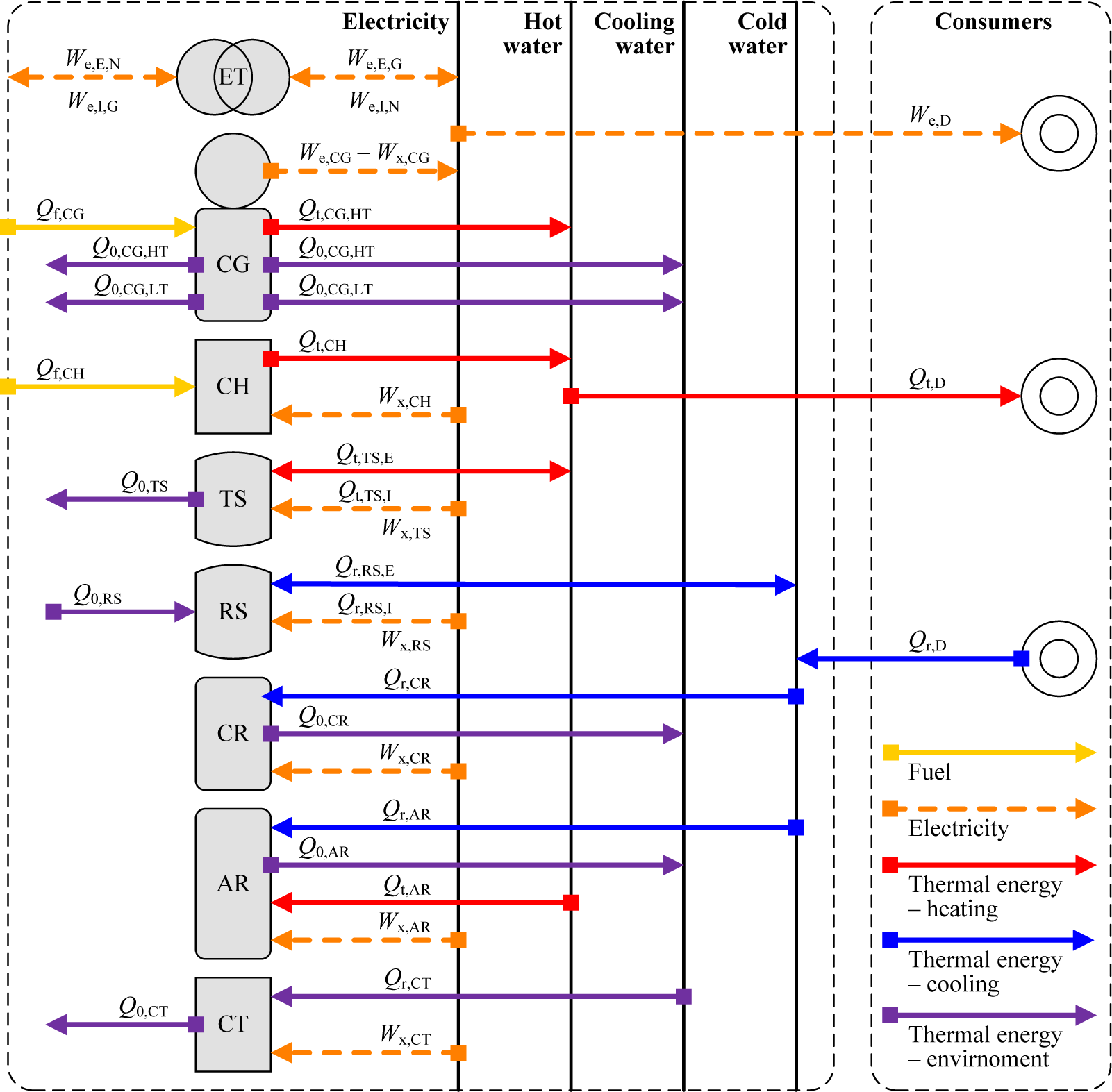
The considered plant might contain the following main types of components: a cogeneration unit (CG), i.e., a reciprocating internal combustion engine or a gas turbine, an additional heating unit, i.e., a hot water boiler (CH), daily heating and cooling storage tanks (TS and RS), an absorption chiller (AR), a compression chiller (CR) and a cooling tower (CT). Larger storage tanks might also be considered, but then it would be desirable to take typical weeks instead of days. System components and energy flows are illustrated in Figure 1. The models and the number of components, as well as their operational strategies are not predefined and should be determined using the presented optimization methodology.

The electricity required for demand satisfaction and operation of the plant components is generated in CGs or imported from the electrical distribution grid via the electrical transformer (ET). Electricity can be exported to the grid via ET. The heating demand and heat required for ARs are satisfied from CGs and CHs. Both are natural gas or biogas fired. Excess heat may be stored in TS and used later. The consumers’ cooling demands are satisfied with ARs and CRs. Only the indirect-fired single-stage ARs are considered here. Both ARs and CRs are water-cooled. If more cooling is produced than required, it can be stored in RS. For both TS and RS, the storage medium is water, which always remains in the liquid state, i.e., there is no phase change. Excess heat from the chillers’ condensers is rejected into the environment via CTs. Excess heat from CGs can also be rejected using CTs or their own coolers with forced convection, which results in additional electricity consumption. It is assumed that high-temperature (HT) heat output from CGs is used for heating and driving ARs, while low-temperature (LT) output is entirely rejected.

This methodology can be extended to include other components such as other types of ARs, air-cooled CRs, electricity storage, photovoltaics, solar thermal heaters, etc.

2.2. Time Frame

The analyzed horizon might be divided into billing periods, that isusually months. In simpler cases, the use of billing periods is not required. The horizon and/or each billing period is represented with one or more typical periods. Each typical period represents an approximation of one or multiple real periods similar in terms of energy demand, energy prices, environment state and other relevant input parameters.

The typical periods are divided into time steps. Here, all of the steps are of the same duration. The fundamental assumptions related to the time steps are:

–

The input parameters, such as energy demand, energy prices and the environment state, are constant during one time step,

–

The operation of each component is stationary during one time step, except eventual short transient start-up and shutdown periods,

–

The load level of each component is constant during one time step,

–

The temperatures of the thermal storage mediums vary during time steps due to charging, discharging and heat losses or gains, but the charging and discharging rates are constant.

The choice of the number of typical periods and the duration of time steps is a matter of compromise between accuracy and efficiency. More typical periods and shorter time steps result in more accurate representations of a real state, but also lead to larger problems that require more time or resources to be solved. The lower bound of time step duration is defined with the requirement that it should be possible to turn on each component to the stationary operation phase during one step.

Here, the analysis is conducted for one year. It is assumed that the year is represented with four typical days with a satisfactory level of accuracy for the purpose of this paper. Each typical day is divided into 24 time steps of 1 h. Longer or shorter steps could also be applied.

2.3. Energy Demand

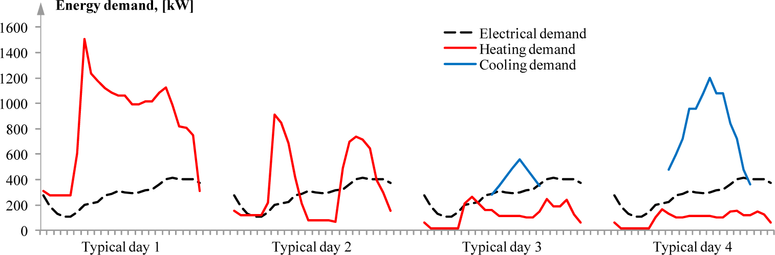
Energy demand profiles for the typical days are illustrated in Figure 2. They are obtained combining the results of the actual on-site measurements of electricity and heat consumption and the detailed hourly simulations of buildings behavior for an entire year. The simulations are performed using the weather data from [43]. Typical Days 1 and 2 represent 103 and 76 cold and mild days during a heating season, respectively, while Days 3 and 4 represent 106 mid-season and 80 summer days.

3. Mathematical Model

The mathematical model is similar to [42,44]. However, here, a more generalized and slightly improved version of the model is presented.

3.1. Input Parameters

The methodology presented in this paper is based on the following input parameters:

–

Data related to the time frame, e.g., billing periods, typical periods count and time step duration,

–

Environment air state—dry and wet bulb temperatures, relative or absolute humidity and pressure—for each time step,

–

Electricity, heating and cooling demands for each time step,

–

Primary energy conversion factors for fuels, imported and exported electricity,

–

The prices of energy commodities—fuels, imported and exported electricity—for each time step,

–

Relevant technical data for each examined component, e.g., nominal capacities and other relevant design properties, the dependence of capacities on surrounding air states and other parameters, off-design data and their dependences on other input parameters, such as surrounding air states, data related to transient operation during start-up and shutdown, etc.,

–

Finances for each component, e.g., the investment and the operation and maintenance (OM) costs,

–

Relevant economic parameters, such as the inflation or discount rates.

3.2. Synthesis and Design Decision Variables

The aim of the presented optimization methodology is to find the best combination of offered components, i.e., to determine the best set of discrete synthesis and design decision variables with respect to the defined objective functions and constraints. These variables can generally be divided into three categories: (a) binary (0–1) non-dimensional variables, indicating whether a component type or model is included in the plant or not; (b) integer non-negative non-dimensional variables indicating the number of the components of a particular model included in the plant; and (c) discrete variables that do not necessarily have a numeric value, indicating which model of a particular type of components is chosen. The mentioned variables define the investment and OM costs, as well as the plant configuration and design later used to find optimal operation regimes. Additionally, the variables defining demand-side energy saving measures might also be included and influence electricity, heating or cooling demand.

3.3. Objective Functions

The objectives of the synthesis and design optimization problem are to achieve: (a) the minimal ATC of the plant; and (b) the minimal annual PEC of the plant.

ATC, expressed in (EUR), include: the annualized investment (equipment owning) cost, the OM costs for all of the components divided into the constant and the variable part, and the costs and the revenues related to energy commodities, i.e., purchased fuel and electricity and sold electricity:

$$\min Z_{\mathrm{T}}=\frac{r}{1-{(1+r)}^{-T}}{Z}_{\mathrm{Inv}}+{\displaystyle \sum _k{Z}_{\mathrm{OM},C,k}+}\underset{¯}{{\displaystyle \sum _i{\displaystyle \sum _j\left({\displaystyle \sum _k{Z}_{\mathrm{OM},V,k}^{i,j}+Z_{\text{Energy}}^{i,j}}\right)+{\displaystyle \sum _u{\dot{\mathrm{\zeta }}}_{\mathrm{e},\mathrm{I},\mathrm{Cap}}^u}{\dot{W}}_{\mathrm{e},\mathrm{I},\mathrm{Cap}}^u}}}$$

(1)

The underlined part of Equation (1) represents the variable costs of the plant (fuel, electricity, variable OM costs), dependent on the chosen operation regime. In order to calculate ATC, the variable costs have to be determined, i.e., the operation regime must be known. When min Z_T is the only objective, the variable costs must be also minimized. For this purpose, the OO problem is defined and solved.

The other objective, annual PEC of the plant, expressed in (kWh), is defined as shown in Equation (2):

$$\min E_{\mathrm{P}}={\displaystyle \sum _i{\displaystyle \sum _j(({\mathrm{\phi }}_{\mathrm{e},\mathrm{I}}^{i,j}{W}_{\mathrm{e},\mathrm{I}}^{i,j}-{\mathrm{\phi }}_{\mathrm{e},\mathrm{E}}^{i,j}{W}_{\mathrm{e},\mathrm{E}}^{i,j})+{\mathrm{\phi }}_{\mathrm{f}}({\displaystyle \sum _{k=1}^{n_{\mathrm{CG}}}{Q}_{\mathrm{f},\mathrm{CG},k}^{i,j}+}{\displaystyle \sum _{k=1}^{n_{\mathrm{CH}}}{Q}_{\mathrm{f},\mathrm{CH},k}^{i,j}}\left)\right)}}$$

(2)

GHGE might be treated as an objective in the same manner, only using different conversion factors.

In this paper, it is assumed that the operation regime is always cost optimal: chosen to provide the best financial outcome for a given set of equipment, i.e., minimal variable costs.

3.4. Operation Optimization

The OO problem is formulated for a known set of synthesis and design decision variables, i.e., for a defined plant. Thus, some details related to the synthesis and design optimization problem have to be used as inputs to the OO problem. As can be seen from Equations (1) and (2), some outputs from the OO problem are used to evaluate the objective functions of the synthesis and design optimization problem.

The OO problem is defined as an MILP problem.

Decision variables

There are two types of decision variables related to the OO problem: (a) binary (0–1) non-dimensional on/off variables, ${\mathrm{\delta }}_k^{i,j}$, for each time step, indicating whether a component k is operating during a time step i,j or not; and (b) semi-continuous variables representing the components’ energy flows, i.e., load levels for each time step, and the TS and RS mediums’ temperatures at the beginning of each time step. The main operation-related decision variables are presented in

Table 1. Summary of the main operation optimization decision variables. CG, cogeneration unit; ET, electrical transformer; CH, hot water boiler; AR, absorption chiller; CR, compression chiller; CT, cooling tower; TS, heating storage tank; RS, cooling storage tank.

Variable	Label	Unit	Lower Bound	Upper Bound
CG on/off	${\mathrm{\delta }}_{\mathrm{CG},k}^{i,j}$	$\forall i,j,k$ –	0	1
CG electricity output	${\dot{W}}_{\mathrm{e},\mathrm{CG},k}^{i,j}$	$\forall i,j,k$ (kW)	${\mathrm{\delta }}_{CG,k}^{i.j}{\dot{W}}_{\mathrm{e},\mathrm{CG},k,\min }^{i,j}$	${\mathrm{\delta }}_{CG,k}^{i.j}{\dot{W}}_{\mathrm{e},\mathrm{CG},k,max}^{i,j}$
CG XGused heat output	${\dot{Q}}_{\mathrm{t},\mathrm{CG},\mathrm{XG},k}^{i,j}$	$\forall i,j,k$(kW)	0	$Q_{t,CG,\mathrm{XG},\mathrm{T},k}^{i.j}/\mathrm{\tau }$
CG rejected useful heat	${\dot{Q}}_{0,\mathrm{CG},\mathrm{HT},k}^{i,j}$	$\forall i,j,k$ (kW)	0	$Q_{t,CG,\mathrm{HT},\max ,k}^{i.j}/\mathrm{\tau }$
ET import on/off	${\mathrm{\delta }}_{\mathrm{ET},\mathrm{I},}^{i,j}$	$\forall i,j$ –	0	$1;1-{\mathrm{\delta }}_{ET,E}^{i.j}(\text{optional})$
ET export on/off	${\mathrm{\delta }}_{\mathrm{ET},\mathrm{E},}^{i,j}$	$\forall i,j$ –	0	$1;{\mathrm{\delta }}_{ET,E}^{i.j}\le {\displaystyle {\sum }_{k=1}^{n_{\mathrm{CG}}}{\mathrm{\delta }}_{CG,k}^{i.j}}(\text{optional})$
ET electricity import (load)	${\dot{W}}_{\mathrm{e},\mathrm{I},\mathrm{N}}^{i,j}$	$\forall i,j$(kW)	0	${\mathrm{\delta }}_{ET,I}^{i.j}{\dot{W}}_{\mathrm{e},\mathrm{I},\mathrm{N},max}^{i,j}$
ET electricity export (load)	${\dot{W}}_{\mathrm{e},\mathrm{E},\mathrm{N}}^{i,j}$	$\forall i,j$ (kW)	0	${\mathrm{\delta }}_{ET,I}^{i.j}{\dot{W}}_{\mathrm{e},\mathrm{E},\mathrm{N},max}^{i,j}$
ET peak electricity import	${\dot{W}}_{\mathrm{e},\mathrm{I},\mathrm{Cap}}^u$	$\forall u$ (kW)	${max}_{i,j}{W}_{\mathrm{e},\mathrm{I},\mathrm{G}}^{i,j}/\mathrm{\tau },\forall i,j\in u$	–
CH on/off	${\mathrm{\delta }}_{\mathrm{CH},k}^{i,j}$	$\forall i,j,k$ –	0	1
CH heat output	${\dot{Q}}_{\mathrm{t},\mathrm{CH},k}^{i,j}$	$\forall i,j,k$ (kW)	${\mathrm{\delta }}_{\mathrm{CH},k}^{i,j}{\dot{Q}}_{\mathrm{t},\mathrm{CH},k,\min }^{i,j}$	${\mathrm{\delta }}_{CH,k}^{i.j}{\dot{Q}}_{\mathrm{t},\mathrm{CH},k,max}^{i,j}$
AR on/off	${\mathrm{\delta }}_{\mathrm{AR},k}^{i,j}$	$\forall i,j,k$ –	0	1
AR cooling effect	${\dot{Q}}_{\mathrm{r},\mathrm{AR},k}^{i,j}$	$\forall i,j,k$(kW)	${\mathrm{\delta }}_{\mathrm{AR},k}^{i,j}{\dot{Q}}_{\mathrm{r},\mathrm{AR},k,\min }^{i,j}$	${\mathrm{\delta }}_{\mathrm{AR},k}^{i,j}{\dot{Q}}_{\mathrm{r},\mathrm{AR},k,max}^{i,j}$
CR on/off	${\mathrm{\delta }}_{\mathrm{CR},k}^{i,j}$	$\forall i,j,k$ –	0	1
CR cooling effect	${\dot{Q}}_{\mathrm{r},\mathrm{CR},k}^{i,j}$	$\forall i,j,k$ (kW)	${\mathrm{\delta }}_{\mathrm{CR},k}^{i,j}{\dot{Q}}_{\mathrm{r},\mathrm{CR},k,\min }^{i,j}$	${\mathrm{\delta }}_{\mathrm{CR},k}^{i,j}{\dot{Q}}_{\mathrm{r},\mathrm{CR},k,max}^{i,j}$
CT on/off	${\mathrm{\delta }}_{\mathrm{CT},k}^{i,j}$	$\forall i,j,k$ –	0	1
CT rejected heat	${\dot{Q}}_{\mathrm{r},\mathrm{CT},k}^{i,j}$	$\forall i,j,k$ (kW)	0	${\mathrm{\delta }}_{\mathrm{CT},k}^{i,j}{\dot{Q}}_{\mathrm{r},\mathrm{CT},k,max}^{i,j}$
TS on/off	${\mathrm{\delta }}_{\mathrm{TS}}^i$	$\forall i$–	0	1
TS heat import (charging)	${\dot{Q}}_{\mathrm{t},\mathrm{TS},\mathrm{I}}^{i,j}$	$\forall i,j$ (kW)	0	${\mathrm{\delta }}_{\mathrm{TS}}^{i,j}{\dot{Q}}_{\mathrm{t},\mathrm{TS},\mathrm{I}max}^{i,j}$
TS heat export (discharging)	${\dot{Q}}_{\mathrm{t},\mathrm{TS},\mathrm{E}}^{i,j}$	$\forall i,j$ (kW)	0	${\mathrm{\delta }}_{\mathrm{TS}}^{i,j}{\dot{Q}}_{\mathrm{t},\mathrm{TS},\mathrm{E}max}^{i,j}$
TS average temperature	$t_{\mathrm{TS}}^{i,j}$	$\forall i,j$ (°C)	$t_{0,\mathrm{TS},}^{i,j}+{\mathrm{\delta }}_{\mathrm{TS}}^i(t_{\mathrm{TS},\min }^{i,j}-t_{0,\mathrm{TS},}^{i,j})$	$t_{0,\mathrm{TS}}^{i,j}+{\mathrm{\delta }}_{\mathrm{TS}}^i(t_{\mathrm{TS},\max }^{i,j}-t_{0,\mathrm{TS}}^{i,j})$
RS on/off	${\mathrm{\delta }}_{\mathrm{RS}}^i$	$\forall i$ –	0	1
RS heat import (discharging)	${\dot{Q}}_{\mathrm{r},\mathrm{RS},\mathrm{I}}^{i,j}$	$\forall i,j$ (kW)	0	${\mathrm{\delta }}_{\mathrm{RS}}^i{\dot{Q}}_{\mathrm{r},\mathrm{RS},\mathrm{I}max}^{i,j}$
RS heat export (charging)	${\dot{Q}}_{\mathrm{r},\mathrm{RS},\mathrm{E}}^{i,j}$	$\forall i,j$ (kW)	0	${\mathrm{\delta }}_{\mathrm{RS}}^i{\dot{Q}}_{\mathrm{r},\mathrm{RS},\mathrm{E},max}^{i,j}$
RS average temperature	$t_{\mathrm{RS}}^{i,j}$	$\forall i,j$ (°C)	$t_{0,\mathrm{RS},}^{i,j}+{\mathrm{\delta }}_{\mathrm{RS}}^i(t_{\mathrm{RS},\min }^{i,j}-t_{0,\mathrm{RS},}^{i,j})$	$t_{0,\mathrm{RS}}^{i,j}+{\mathrm{\delta }}_{\mathrm{RS}}^i(t_{\mathrm{RS},\max }^{i,j}-t_{0,\mathrm{RS}}^{i,j})$

. Generally, a semi-continuous variable, $x_k^{i,j}$, is limited with lower and upper bounds, $x_{k,\min }^{i,j}$ and $x_{k,max}^{i,j}$, if the related ${\mathrm{\delta }}_k^{i,j}$ is one, and has another value, $x_k^{\ast i,j}$, otherwise: $x_k^{\ast i,j}+{\mathrm{\delta }}_k^{i,j}(x_{k,\min }^{i,j}-x_k^{\ast i,j})\le x_k^{i,j}\le x_k^{\ast i,j}+{\mathrm{\delta }}_k^{i,j}(x_{k,max}^{i,j}-x_k^{\ast i,j})$, for each time step i,j. The bounds depend on the model and the nominal capacity of a component, but also on air temperature, pressure, some design parameters, etc. However, they, as well as $x_k^{\ast i,j}$, are considered as the inputs to the OO problem.

Additional variables

In addition to the decision variables summarized in Table 1, other variables are introduced in order to make the model clearer, easier to understand and less error-prone during software implementation. These additional variables are not treated as decisions, but as their linear functions, i.e., expressions. As such, they do not represent any overhead to the computationally-intensive process of OO, since they are directly inserted into the existing constraints and objectives without requiring the introduction of new decision variables or constraints.

First, having in mind the assumption of stationary operation during each time step, for each decision variable ${\dot{X}}_k^{i,j}$ from Table 1 that is expressed in (kW) and related to a specific energy flow, i.e., a load level, an additional variable $X_k^{i,j}$, in (kWh), is introduced, such that, $X_k^{i,j}={\dot{X}}_k^{i,j}\mathrm{\tau }$, where τ is the time step in (h). Here, τ = 1 h. Other energy flows for each component k and each time step i, j are represented with the additional variables, $Y_k^{i,j}$, expressed in (kWh). They are formulated as linear functions of the related decision variables and summarized in

Table 2. Summary of the main additional variables representing energy flows, given in (kWh).

Variable	Label	Variable	Label
CG electricity output	$W_{\mathrm{e},\mathrm{CG},k}^{i,j}$	AR cooling effect	$Q_{\mathrm{r},\mathrm{AR},k}^{i,j}$
CG XG used heat output	$Q_{\mathrm{t},\mathrm{CG},\mathrm{XG},k}^{i,j}$	AR heat input	$Q_{\mathrm{t},\mathrm{AR},k}^{i,j}$
CG rejected useful heat	$Q_{0,\mathrm{CG},\mathrm{HT},k}^{i,j}$	AR auxiliary electricity input	$W_{\mathrm{x},\mathrm{AR},k}^{i,j}$
CG XG total available heat	$Q_{\mathrm{t},\mathrm{CG},\mathrm{XGT},k}^{i,j}$	AR rejected heat	$Q_{0,\mathrm{AR},k}^{i,j}$
CG engine cooling heat at HT	$Q_{\mathrm{t},\mathrm{CG},\mathrm{HT},k}^{i,j}$	CR cooling effect	$Q_{\mathrm{r},\mathrm{CR},k}^{i,j}$
CG engine cooling heat at LT	$Q_{\mathrm{t},\mathrm{CG},\mathrm{LT},k}^{i,j}$	CR electricity input	$W_{\mathrm{r},\mathrm{CR},k}^{i,j}$
CG fuel input	$Q_{\mathrm{f},\mathrm{CG},k}$	CR rejected heat	$Q_{0,\mathrm{CR},k}^{i,j}$
CG auxiliary electricity input	$W_{\mathrm{x},\mathrm{CG},k}^{i,j}$	CT rejected heat (input)	$Q_{\mathrm{r},\mathrm{CT},k}^{i,j}$
ET net electricity import (load)	$W_{\mathrm{e},\mathrm{I},\mathrm{N}}^{i,j}$	CT electricity input	$W_{\mathrm{x},\mathrm{CT},k}^{i,j}$
ET net electricity export (load)	$W_{\mathrm{e},\mathrm{E},\mathrm{N}}^{i,j}$	TS heat import (storage charging)	$Q_{\mathrm{t},\mathrm{TS},\mathrm{I}}^{i,j}$
ET gross electricity import (source)	$W_{\mathrm{e},\mathrm{I},\mathrm{G}}^{i,j}$	TS heat export (storage discharging)	$Q_{\mathrm{t},\mathrm{TS},\mathrm{E}}^{i,j}$
ET gross electricity export (source)	$W_{\mathrm{e},\mathrm{E},\mathrm{G}}^{i,j}$	TS auxiliary electricity input	$W_{\mathrm{x},\mathrm{TS}}^{i,j}$
CH heat output	$Q_{\mathrm{t},\mathrm{CH},k}^{i,j}$	RS heat import (storage discharging)	$Q_{\mathrm{r},\mathrm{RS},\mathrm{I}}^{i,j}$
CH fuel input	$Q_{\mathrm{f},\mathrm{CH},k}^{i,j}$	RS heat export (storage charging)	$Q_{\mathrm{r},\mathrm{RS},\mathrm{E}}^{i,j}$
CH auxiliary electricity input	$W_{\mathrm{x},\mathrm{CH},k}^{i,j}$	RS auxiliary electricity input	$W_{\mathrm{x},\mathrm{RS}}^{i,j}$

.

When the stationary operation assumption holds, it is often sufficient to assume a linear dependence:

$${\dot{Y}}_k^{i,j}={\displaystyle \sum _{l=1}^{n_X}{a}_{k,l}^{i,j}{\dot{X}}_{k,l}^{i,j}+b_k^{i,j}{\mathrm{\delta }}_k^{i,j},0\le {\mathrm{\delta }}_k^{i,j}}{\dot{X}}_{k,l,\min }^{i,j}\le {\dot{X}}_{k,l}^{i,j}\le {\mathrm{\delta }}_k^{i,j}{\dot{X}}_{k,l,max}^{i,j},l=1,2,\dots ,n_X\forall i,j$$

(3)

where ${\dot{Y}}_k^{i,j}$ is an energy flow, in (kW), n_X is the number of related semi-continuous decision variables, while $a_{k,l}^{i,j}$ and $b_k^{i,j}$ are the linear regression coefficients, usually measured or provided by the manufacturers of components for each model separately, which might depend on various input parameters, such as the air temperature. In any case, they are considered as inputs to the OO problem. This approach allows the precise and detailed consideration of off-design and part-load performance characteristics and their variation with the environment temperature and other relevant input data.

If the linear function from Equation (3) is not accurate enough, a piecewise linear approximation of a relation between ${\dot{Y}}_k^{i,j}$ and any ${\dot{X}}_{k,l}^{i,j}$ might be established. It can be done in several ways, one of which will be presented here. In order to approximate a semi-continuous function y = f (x), where ${\mathrm{\delta }}_k^{i,j}{x}_{\min }\le x\le {\mathrm{\delta }}_k^{i,j}{x}_{max}$, n sampling points are chosen, with coordinates (X₁,Y₁), (X₂,Y₂),…,(X_n,Y_n), such that $x_{\min }=X_1\le X_2\le \cdots \le X_n=x_{max}$. Also, n auxiliary continuous nonnegative decision variables λ₁,λ₂,…,λ_n are introduced, such that they form a special ordered set of Type 2 (SOS2), i.e., an ordered set of nonnegative variables of which only two successive might be non-zero. Then, the linear approximation of y, y_L, the decision variable x and the additional constraints to the problem are:

$$y_{\mathrm{L}}={\displaystyle \sum _{q=1}^n{Y}_q{\mathrm{\lambda }}_q},x={\displaystyle \sum _{q=1}^n{X}_q{\mathrm{\lambda }}_q},{\displaystyle \sum _{q=1}^n{\mathrm{\lambda }}_q={\mathrm{\delta }}_k^{i,j},}({\mathrm{\lambda }}_1,{\mathrm{\lambda }}_2,\dots ,{\mathrm{\lambda }}_n):\mathrm{SOS}2$$

(4)

When using this approach to represent a relation between ${\dot{Y}}_k^{i,j}$ and ${\dot{X}}_{k,l}^{i,j}$, ${\dot{X}}_{k,l}^{i,j}$

may be optionally eliminated from the set of decision variables and $X_{k,l}^{i,j}$ and $Y_k^{i,j}$ expressed directly as functions of λ₁,λ₂,…,λ_n.

The number of the sample points can vary depending on the desired accuracy. A bigger number of points leads to higher accuracy, but also to larger problems. The coordinates of the sample points might vary with time steps and depend on input data, just as the values of the coefficients $a_{k,l}^{i,j}$ and $b_k^{i,j}$.

In addition to stationary operation, some corrections are used to take into account transient non-stationary start-up and shutdown processes. A complete expression for defining any energy flow $Y_k^{i,j}$, expressed in (kWh), related to a component k and a time step i, j is:

$$Y_k^{i,j}=\stackrel{\text{Stationary operation}}{\overbracket{({\displaystyle \sum }_{l=1}^{n_X}{a}_{k,l}^{i,j}{\dot{X}}_{k,l}^{i,j}+b_k^{i,j}{\mathrm{\delta }}_{k,l}^{i,j})\mathrm{\tau }}}+\stackrel{\text{Start-up correction}}{\overbracket{{\displaystyle \sum }_{l=1}^{n_{\mathrm{\sigma }}}{Y}_{\mathrm{\sigma },k,l}^{i,j}\underset{¯}{{\mathrm{\delta }}_k^{i,j}{\displaystyle \prod }_{q=1}^l(1-{\mathrm{\delta }}_k^{i,j-q})}}}+\stackrel{\text{Shutdown correction}}{\overbracket{Y_{\mathrm{\varsigma },k,1}^{i,j}\underset{¯}{{\mathrm{\delta }}_k^{i,j}(1-{\mathrm{\delta }}_k^{i,j+1})}}}\forall i,j$$

(5)

where n_σ is the number of previous time steps taken into account, while $Y_{\mathrm{\sigma },k,l}^{i,j}$ and $Y_{\mathrm{\varsigma },k,l}^{i,j}$ are the correctedamounts of energy related to start-ups and shutdowns, in (kWh), that might depend on input data and vary with time. These corrections are often neglected in the literature, while one previous time step is considered in [16,45]. Here, a more generalized approach is presented, but three previous time steps are actually observed. In order to obtain linear relationships instead of the products of the binary variables in Equation (5), for each time step i, j, the following auxiliary binary variables are introduced to replace the underlined terms:

$${\mathrm{\sigma }}_{k,1}^{i,j}={\mathrm{\delta }}_k^{i,j}(1-{\mathrm{\delta }}_k^{i,j-1}),{\mathrm{\sigma }}_{k,l}^{i,j}={\mathrm{\sigma }}_{k,l-1}^{i,j}(1-{\mathrm{\delta }}_k^{i,j-1}),l=2,3,\dots n_{\mathrm{\sigma }},{\mathrm{\varsigma }}_k^{i,j}={\mathrm{\delta }}_k^{i,j}(1-{\mathrm{\delta }}_k^{i,j+1})\forall i,j$$

(6)

as well as the additional inequality constraints related to them:

$${\mathrm{\sigma }}_{k,1}^{i,j}\le {\mathrm{\delta }}_k^{i,j},{\mathrm{\sigma }}_{k,1}^{i,j}\le 1-{\mathrm{\delta }}_k^{i,j-1},{\mathrm{\sigma }}_{k,1}^{i,j}\ge {\mathrm{\delta }}_k^{i,j}-{\mathrm{\delta }}_k^{i,j-1}i,j$$

(7a)

$${\mathrm{\sigma }}_{k,1}^{i,j}\le {\mathrm{\sigma }}_{k,l-1}^{i,j},{\mathrm{\sigma }}_{k,1}^{i,j}\le 1-{\mathrm{\delta }}_k^{i,j-1},{\mathrm{\sigma }}_{k,1}^{i,j}\ge {\mathrm{\sigma }}_{k,l-1}^{i,j}-{\mathrm{\delta }}_k^{i,j-1}l=2,3,\dots ,n_{\mathrm{\sigma }}\forall i,j$$

(7b)

$${\mathrm{\varsigma }}_k^{i,j}\le {\mathrm{\delta }}_k^{i,j},{\mathrm{\varsigma }}_k^{i,j}\le 1-{\mathrm{\delta }}_k^{i,j+1},{\mathrm{\varsigma }}_k^{i,j}\ge {\mathrm{\delta }}_k^{i,j}-{\mathrm{\delta }}_k^{i,j+1}\forall i,j$$

(7c)

Basically, ${\mathrm{\sigma }}_{k,1}^{i,j}$ shows whether a component k is turned on at the beginning of a time step i, j, ${\mathrm{\sigma }}_{k,l}^{i,j}$ shows whether it is turned on after l or more time steps of being off; and ${\mathrm{\zeta }}_k^{i,j}$ shows whether it is turned off at the end of the step i,j. A similar approach is proposed in [18] and a slightly different one in [17].

OM costs, given in (EUR), are also expressed as linear functions of decision variables for each component k. Generally, they consist of constant and variable costs [46]:

$$Z_{\mathrm{OM},\mathrm{T},k}=Z_{\mathrm{OM},C,k}+Z_{\mathrm{OM},\mathrm{V},k}=Z_{\mathrm{OM},C,k}+{\displaystyle \sum _i{\displaystyle \sum _j{Z}_{\mathrm{OM},V,k}^{i,j}}}$$

(8)

Constant OM costs depend only on the model of the component, while variable ones depend on the operation parameters, such as energy flows and the time of operation:

$$Z_{\mathrm{OM},V,k}^{i,j}=\left({\displaystyle \sum _{l=1}^{n_X}{\mathrm{\alpha }}_{k,l}^{i,j}{\dot{X}}_{k,l}^{i,j}+{\mathrm{\beta }}_k^{i,j}{\mathrm{\delta }}_k^{i,j}}\right)\mathrm{\tau }\forall i,j$$

(9)

where ${\mathrm{\sigma }}_{k,1}^{i,j}$ and ${\mathrm{\beta }}_k^{i,j}$ are the linear regression coefficients, while ${\dot{X}}_{k,1}^{i,j}$ represent n_X decision variables used to define OM costs of a component k during a time step i,j, in (kW). The additional costs related to start-ups and shutdowns might also be included.

Energy-related cash flows for each time step i,j include the incomes for sold electricity and the outcomes for purchased electricity and fuel:

$$Z_{\text{Energy}}^{i,j}={\mathrm{\zeta }}_{\mathrm{e},}^{i,j}{W}_{\mathrm{e},}^{i,j}-{\mathrm{\zeta }}_{\mathrm{e},\mathrm{E}}^{i,j}{W}_{\mathrm{e},\mathrm{E}}^{i,j}+{\mathrm{\zeta }}_{\mathrm{f},\mathrm{CG}}^{i,j}{\displaystyle \sum _{k=1}^{n_{\mathrm{CG}}}{Q}_{\mathrm{f},\mathrm{CG},k}^{i,j}+{\mathrm{\zeta }}_{\mathrm{f},\mathrm{CH}}^{i,j}}{\displaystyle \sum _{k=1}^{n_{\mathrm{CH}}}{Q}_{\mathrm{f},\mathrm{CH},k}^{i,j}}\forall i,j$$

(10)

Objective function

It is assumed that the energy supply system of interest is operating in the financially optimal mode, i.e., generating minimal variable costs that include all of the cash flows depending on the operation regimes: the variable OM costs, the energy costs and the peak power costs. Thus, the objective of the OO problem is defined as:

$$\min Z_{\mathrm{v}}={\displaystyle \sum _i{\displaystyle \sum _j\left({\displaystyle \sum _k{Z}_{\mathrm{OM},V,k}^{i,j}+}{Z}_{\text{Energy}}^{i,j}\right)+{\displaystyle \sum _u{\dot{\mathrm{\zeta }}}_{\mathrm{e},\mathrm{I},\mathrm{Cap}}^u}{\dot{W}}_{\mathrm{e},\mathrm{I},\mathrm{Cap}}^u}}$$

(11)

Constraints

Some constraints of the OO problem are already listed in Table 1. They are related to the basic lower and upper bounds of the decision variables. In addition to them and to the auxiliary constraints from Equations (7), energy balances and other limitations on the energy flows should be included. For example, it may be useful to limit exported electricity with the amount generated by the system:

$$W_{\mathrm{e},\mathrm{E},\mathrm{G}}^{i,j}\le {\displaystyle \sum _{k=1}^{n_{\mathrm{CG}}}{W}_{\mathrm{e},\mathrm{CG},k}^{i,j}\forall i,j}$$

(12)

Total heat removed using CTs should match the heat rejected from ARs and CRs and, optionally, CGs (if they do not have coolers). It is assumed that LT heat from CGs is rejected entirely, thus:

$${\displaystyle \sum _{k=1}^{n_{\mathrm{CT}}}{Q}_{\mathrm{r},\mathrm{CT},k}^{i,j}=}{\displaystyle \sum _{k=1}^{n_{\mathrm{AR}}}{Q}_{0,\mathrm{AR},k}^{i,j}+}{\displaystyle \sum _{k=1}^{n_{\mathrm{CR}}}{Q}_{0,\mathrm{CR},k}^{i,j}+{\displaystyle \sum _{k=1}^{n_{\mathrm{CG}}}(Q_{0,\mathrm{CG},\mathrm{HT},k}^{i,j}+Q_{\mathrm{t},\mathrm{CG},\mathrm{LT},k}^{i,j})\forall i,j}}$$

(13)

Energy balances of TS and RS imply the relation to the mediums’ temperatures at the beginning of each of two consecutive time steps:

$$t_{\mathrm{TS}}^{i,j+1}=\begin{array}{l}\left(\frac{a_{\mathrm{t},\mathrm{TS},\mathrm{I}}^{i,j}{\dot{Q}}_{\mathrm{t},\mathrm{TS},\mathrm{I}}^{i,j}-a_{\mathrm{t},\mathrm{TS},\mathrm{E}}^{i,j}{\dot{Q}}_{\mathrm{t},\mathrm{TS},\mathrm{E}}^{i,j}+b_{\mathrm{t},\mathrm{TS}}^{i,j}{\mathrm{\delta }}_{0,\mathrm{TS}}^{i,j}}{U_{\mathrm{TS}}{A}_{\mathrm{TS}}}\right)(1-\exp (-\frac{U_{\mathrm{TS}}{A}_{\mathrm{TS}}\mathrm{\tau }}{m_{\mathrm{TS}}{c}_{\mathrm{TS}}}\left)\right)\\ +t_{\mathrm{TS}}^{i,j}\exp =(-\frac{U_{\mathrm{TS}}{A}_{\mathrm{TS}}\mathrm{\tau }}{m_{\mathrm{TS}}{c}_{\mathrm{TS}}})+(1-{\mathrm{\delta }}_{\mathrm{TS}}^i)(t_{0,\mathrm{TS}}^{i,j+1}-t_{0,\mathrm{TS}}^{i,j})\forall i,j\end{array}$$

(14)

$$t_{\mathrm{RS}}^{i,j+1}=\begin{array}{l}(\frac{a_{\mathrm{r},\mathrm{RS},\mathrm{I}}^{i,j}{\dot{Q}}_{\mathrm{r},\mathrm{RS},\mathrm{I}}^{i,j}-a_{\mathrm{r},\mathrm{RS},\mathrm{E}}^{i,j}{\dot{Q}}_{\mathrm{r},\mathrm{RS},\mathrm{E}}^{i,j}+b_{\mathrm{r},\mathrm{RS}}^{i,j}{\mathrm{\delta }}_{\mathrm{RS}}^{i,j}}{U_{\mathrm{TS}}{A}_{\mathrm{TS}}}+t_{0,\mathrm{RS}}^{i,j})(1-\exp (-\frac{U_{\mathrm{RS}}{A}_{\mathrm{RS}}\mathrm{\tau }}{m_{\mathrm{RS}}{c}_{\mathrm{RS}}}\left)\right)\\ +t_{\mathrm{RS}}^{i,j}\exp =(-\frac{U_{\mathrm{RS}}{A}_{\mathrm{RS}}\mathrm{\tau }}{m_{\mathrm{RS}}{c}_{\mathrm{RS}}})+(1-{\mathrm{\delta }}_{\mathrm{RS}}^i)(t_{0,\mathrm{RS}}^{i,j+1}-t_{0,\mathrm{RS}}^{i,j})\forall i,j\end{array}$$

(15)

These equations are derived by integrating the energy balances in the differential form over time and assuming constant the storage overall heat transfer coefficient, U, and the area, A, as well as the medium mass, m, and the heat capacity, c. The last terms on the right-hand sides of Equations (14) and (15) are not derived from the energy balances, but added to artificially maintain the storage and environment temperatures equal for the typical periods when a storage is not used, i.e., ${\mathrm{\delta }}_{\mathrm{TS}}^i=0$ or ${\mathrm{\delta }}_{\mathrm{RS}}^i=0$, and thus, the temperature is not relevant. When storage is used, this term is zero.

The demand-satisfaction constraints are given in Equations (16)–(18), which ensure the possibility of the plant to satisfy consumers’ electricity, heating and cooling demands during each observed time step i, j:

$$W_{\mathrm{e},\mathrm{D}}^{i,j}=\begin{array}{l}{W}_{\mathrm{e},\mathrm{I},\mathrm{N}}^{i,j}-W_{\mathrm{e},\mathrm{E},\mathrm{G}}^{i,j}+{\displaystyle \sum _{k=1}^{n_{\mathrm{CG}}}(W_{\mathrm{e},\mathrm{CG},\mathrm{k}}^{i,j}-W_{\mathrm{x},\mathrm{CG},k}^{i,j})-}{\displaystyle \sum _{k=1}^{n_{\mathrm{CH}}}{W}_{\mathrm{x},\mathrm{CH},k}^{i,j}-W_{\mathrm{x},\mathrm{TS}}^{i,j}}\\ -{\displaystyle \sum _{k=1}^{n\mathrm{AR}}{W}_{\mathrm{x},\mathrm{AR},k}^{i,j}-}{\displaystyle \sum _{k=1}^{n_{\mathrm{CR}}}{W}_{\mathrm{x},\mathrm{CR},k}^{i,j}-{\displaystyle \sum _{k=1}^{n_{\mathrm{CT}}}{W}_{\mathrm{x},\mathrm{CT},k}^{i,j}}-W_{\mathrm{x},\mathrm{RS}}^{i,j}\forall i,j}\end{array}$$

(16)

$$Q_{\mathrm{t},\mathrm{D}}^{i,j}=\begin{array}{l}{\displaystyle \sum _{k=1}^{n_{{}_{\mathrm{CG}}}}(Q_{\mathrm{t},\mathrm{CG},\mathrm{XG},k}^{i,j}+Q_{\mathrm{t},\mathrm{CG},\mathrm{HT},k}^{i,j}-Q_{0,\mathrm{CG},\mathrm{HT},k}^{i,j})+}{\displaystyle \sum _{k=1}^{n_{\mathrm{CH}}}{Q}_{\mathrm{t},\mathrm{CH},k}^{i,j}}\\ -{\displaystyle \sum _{k=1}^{n_{\mathrm{AR}}}{Q}_{\mathrm{t},\mathrm{AR},k}^{i,j}+}{Q}_{\mathrm{t},\mathrm{TS},\mathrm{E}}^{i,j}-Q_{\mathrm{t},\mathrm{TS},\mathrm{I}}^{i,j}\forall i,j\end{array}$$

(17)

$$Q_{\mathrm{r},\mathrm{D}}^{i,j}={\displaystyle \sum _{k=1}^{n\mathrm{AR}}{Q}_{\mathrm{r},\mathrm{AR},k}^{i,j}+}{\displaystyle \sum _{k=1}^{n\mathrm{CR}}{Q}_{\mathrm{r},\mathrm{CR},k}^{i,j}+}{Q}_{\mathrm{r},\mathrm{RS},\mathrm{I}}^{i,j}-Q_{\mathrm{r},\mathrm{RS},\mathrm{E}}^{i,j}\forall i,j$$

(18)

It is also possible to add other, problem-specific constraints, e.g., legal [20], the boundaries on load-level variation for some components [47], the minimum number of the time steps for which the component can be on or off [16], the environmental impact of the system, etc.

Initial and final conditions

These conditions are important for time-coupling constraints. Here, the assumption is that each typical period is preceded and followed by the identical period, with equal input parameters and, consequently, the same operation regime. Thus, the initial conditions are related to the end and the final to the beginning of the observed period. For example, if n_τ is the number of time steps per period, we assume that the time step i,0 is preceded by the step i,n_τ − 1. Generally, the correct indexes of the step i,j ± n, which occurs n steps after or before i,j, are determined as i, (j ± n) mod n_τ, if the division remainder is calculated in a way to always be positive.

4. Methodology

The methodology presented here is based on the conceptual decomposition [2] and the combination of MH methods and MILP.

4.1. Conceptual Decomposition

The problem is decomposed into two levels of optimization, similar to [48]:

• synthesis and design optimization,

• operation optimization.

Thus, two nested problems are obtained: (a) the main problem of synthesis and design optimization and (b) the inner problem of OO. The synthesis and design decision variables considered here are discrete and related only to the choice of the models and the number of the components to be installed, making the main problem combinatorial. Eventually, demand-side energy-saving measures might be also chosen using discrete variables. The operation-related decision variables are binary and semi-continuous. The OO problem is defined as an MILP problem.

4.2. Solution Procedure

MH methods are used to find the optimal or near-optimal combination of the synthesis and design variables. There are many such methods, but what is common to all of them is that the value of the objective function is calculated repeatedly, many times, for various candidate solutions, hopefully approaching the optimum. Every time the value of the objective function is to be calculated for some evaluated set of the synthesis and design variables, the optimal operation regime is determined, i.e., the OO problem is constructed and solved using an appropriate method, e.g., the branch-and-cut method. Solving MILP OO problems is computationally by far the most intensive part of this process.

The following procedure is used to evaluate each combination of the synthesis and design variables:

• Check in the database of already evaluated vectors if this combination is saved. If yes, simply find the appropriate values of the objective functions and go to Step 5. Otherwise, go to Step 2.

• Define and solve the OO problem following this procedure:

(a)

Create the OO problem with respect to the evaluated plant parameters, i.e., the given synthesis and design variables, but also with respect to other input data: energy demand, energy prices, part-load performance characteristics of the examined components, the environment state, etc.

(b)

Solve this problem using the MILP solver (in this case, based on the branch-and-cut method).

(c)

Remember the obtained values of the operation variables and the objectives.

(d)

Free the computer resources used to solve this problem.

• Calculate the values of the objective functions of the synthesis and design the optimization problem using the input data and the solution of OO, e.g., using Equations (1) and (2).

• Save the values of the decision variables and the objective functions in the database of already evaluated vectors (combinations).

• Return the value(s) of the objective function(s).

The construction of the OO problem for each examined set of the synthesis and design variables is one of the main aspects of this approach. It is the procedure that is performed precisely and quickly using the appropriate software tool connected to both the energy-system-related software component and the MILP solver. It is not computationally intensive compared to solving this problem; on the contrary, it is actually negligible (it takes less than 1% of the total solving time). On the other hand, it might significantly improve the flexibility in mathematical modeling and lead to the reduction of the OO problem size and, consequently, the computation time.

Using the database of already evaluated vectors and Steps 1 and 4 are not necessary. However, this is useful, because it leads to significantly shorter computation times. When using MH methods, it often happens that the same combination of the synthesis and design variables is evaluated multiple times during the same run, especially in the later phases of the algorithm, when the optimal solution is close to being or already found. This way, the unnecessary operations 2 and 3 can be avoided, especially the calls to the MILP solver requesting it to solve the problem that has already been solved.

4.3. Optimization Methods

The optimization methods used to find the optimal values of the synthesis and design variables are:

–

genetic algorithms (GNA),

–

particle swarm optimization (PSO),

–

ant colony optimization (ACO),

–

simulated annealing (SAN),

–

harmony search (HMS),

–

tabu search (TBS).

All of these methods are very convenient for discrete optimization, except PSO. This was originally created for continuous problems, but several attempts have been made to adjust it to discrete ones, such as [49,50]. However, here, the algorithm is used as described in [17], and the obtained coordinates decimal values are simply rounded to the nearest integers.

This methodology might involve other approaches for the determination of operation regimes. First, methods other than the branch-and-cut might be used to solve the OO MILP problem. This problem might also be defined as nonlinear and solved using some appropriate method. It is also possible to use the moving-horizon short-term optimization approach [10,11]. If it is satisfactory for the user, operation regimes might be just assumed, without doing optimization at all, etc.

4.4. Decomposition over Time

If typical periods are used, it might be possible to decompose the inner OO problem over time. If there are no constraints coupling multiple billing periods, such as allowed environmental impact per year, the OO problem might be divided and solved for each billing period separately. Similarly, if there are no constraints coupling the typical periods from the same billing period, such as the ones that involve the peak imported electricity, ${\dot{W}}_{\mathrm{e},\mathrm{I},\mathrm{Cap}}^u$, the problem might be solved for each typical period separately. This decomposition usually results in the reduction of the computational time and effort required to solve the problem. Moreover, if the OO problem for one period is infeasible or unbounded, the examined combination of synthesis/design variables can be rejected without solving the problems for other periods.

4.5. Multiple Objectives Consideration

The result of the MO optimization is usually not a single solution, but a set of the Pareto optimal solutions, i.e., the solutions that cannot be improved with respect to one objective value without deteriorating at least one of the other values of the objective functions [51].

In order to obtain the Pareto optimal solutions of the MO version of this problem, the epsilon-constraint method is used. Only one objective function is kept, while all others are constrained with some constant values. These bounds are parametrically varied, and the optimization procedure is repeated. The primary objective here is to minimize ATC, while the secondary objective, PEC, is constrained with target values using the inequality constraints.

4.6. Flexibility-Related Considerations

MH methods and the structural decomposition allow a high degree of flexibility when defining the mathematical model. The overall objective functions and the constraints not directly related to the operation variables do not have to be linear. One might use numerical procedures to determine the value of an objective function (e.g., the internal rate of return). Conflicting objectives on different optimization levels, e.g., the variable costs and PEC, are acceptable. Soft constraints might be defined and treated in many ways. As already mentioned, the choice of the approaches for solving OO problems is wide, and if selected, the typical-periods-based approach is suitable for usually beneficial decomposition over time.

4.7. Software Solution

The full description of the software used here is beyond the scope of this paper. It should be underlined that it performs three main tasks: (a) creates the OO problem based on the set of components included in the plant; (b) solves optimization problems; and (c) calculates output parameters. Its most important elements are: the main element related to the energy system and its components that stores performance data and other inputs and defines functions for calculations, the solvers for six MH methods and the component that creates the OO problems and communicates with the external MILP solvers, i.e., sends them the requests to solve the defined problems, accepts the solutions and provides them to the main element. The external MILP solvers used are Gurobi Optimizer [52], Solver Foundation [53] and LP Solve [54].

This software solution, named ESO-MS, is an object-oriented multi-platform tool, developed in the C# programming language by the first author of this paper. It works on the .Net and Mono frameworks. The suitability of the object-oriented approach for this type of software is stressed in [16,55].

5. Results and Discussion

The proposed approach is applied for the optimization of an energy plant that might supply a residential settlement in Niš, Serbia. The analysis is performed for one typical year within the horizon of 15 years, the annual inflation rate of 8% and the neglected residual value of the equipment after the horizon observed. The considered options for the synthesis and design decision variables—the models and the number of units—are given in

Table 3. Synthesis and design decision variables and characteristic solution values.

Variable	Values					Solutions
	0	1	2	3	4	A	B	C
CG model	M0 (315 kWe)	M1 (460 kWe)	M2 (570 kWe)	M3 (803 kWe)	M4 (1,464 kWe)	3	4	4
CGs units count	–	1	2	–	–	1	1	1
CHs units count	0	1	2	3	4	0	1	0
TS size	M0 (4 t)	M1 (40 t)	M2 (80 t)	M0 (160 t)	M4 (400 t)	4	4	4
AR model	M0 (380 kWr)	M1 (868 kWr)	M2 (1,402 kWr)	M3 (2,595 kWr)	M4 (3,021 kWr)	0	0	0
CR model	M0 (236 kWr)	M1 (367 kWr)	M2 (455 kWr)	M3 (641 kWr)	M4 (842 kWr)	3	0	3
CRs units count	0	1	2	3	4	1	4	1
RS size	10% of TS mass	30% of TS mass	50% of TS mass	70% of TS mass	90% of TS mass	4	2	4
CT model	M0 (500 kWt)	M1 (1,000 kWt)	–	–	–	1	1	1
CTs units count	–	1	2	–	–	1	1	1

. The price of natural gas is 0.04 EUR kWh⁻¹ based on the lower heating value; the price of purchased electricity is 0.10 EUR kWh⁻¹ during days (from 7 to 23 h) and 0.025 EUR kWh⁻¹ during nights (from 23 to 7 h); and the price of sold electricity is 0.10 EURkWh⁻¹.

5.1. Optimal Solutions

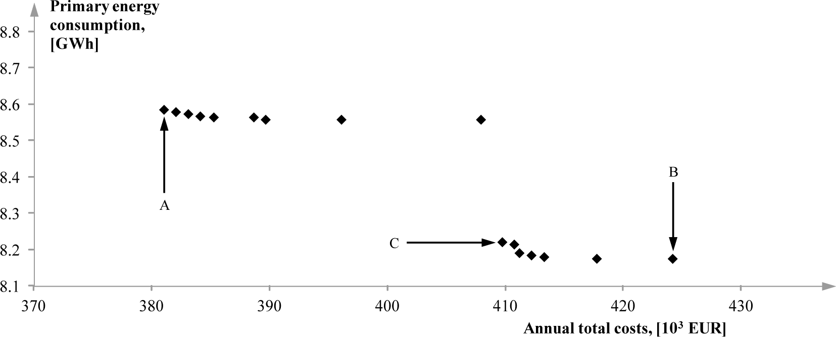
The solution with minimal ATC is denoted as Solution A, and the solution with minimal PEC is Solution B. Another solution, C, appears to be a good compromise between A and B. It differs from A only in the CG size. The values of the decision variables for these solutions are shown in Table 3 and those of the corresponding objective functions in

Table 4. Values of the objective functions for Solutions A, B and C.

Objective Function	Solution A	Solution B	Solution C
Annual total costs, (EUR)	381,068	424,198	409,752
Primary energy consumption, (MWh)	8,584.4	8,174.1	8,219.7

. All of the Pareto optimal solutions closer to A have one CG of 803 kW_e, while the ones closer to B have one CG of 1,464 kW_e. All of them have the largest offered TS. The regimes ensure cost optimal operation for given sets of equipment and are characterized with the extensive use of CG, TS and RS, the absence of heat rejection and low utilization of AR.

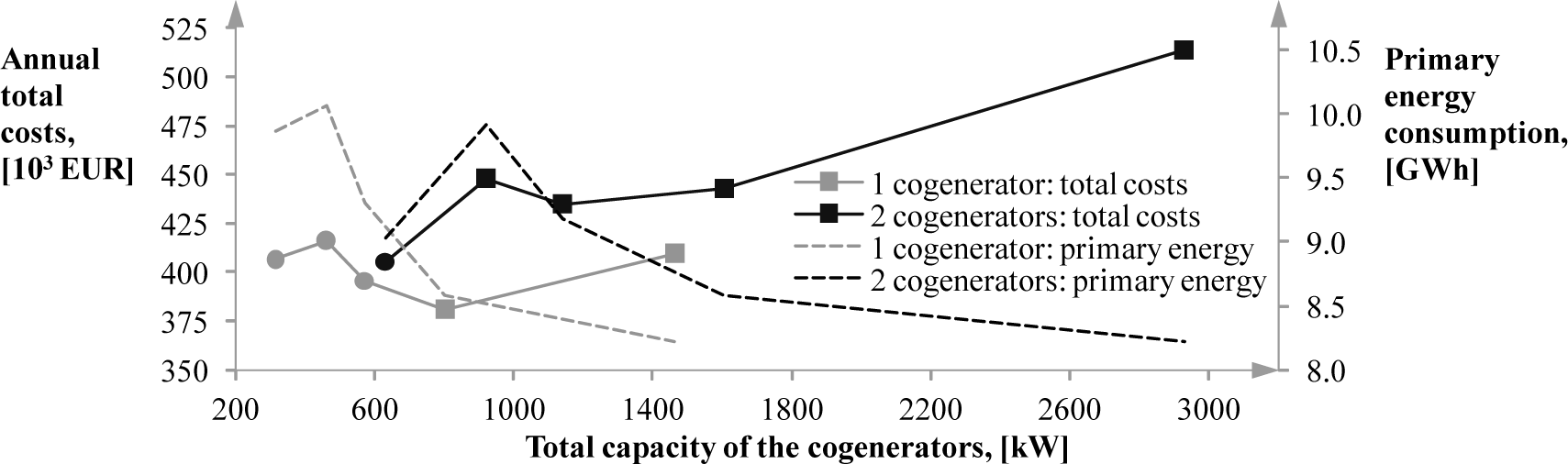
The solutions with fewer CGs are preferable. They generally require lower investment costs for the same nominal capacities, and in some cases, units of higher capacities are more efficient than smaller ones. Solutions with two or more units are more flexible in operation, but in this case, the desired flexibility is ensured with TS and RS. The significant dependence of ATC and PEC on the models and the number of CGs is illustrated in Figure 4. It is related to Solution A with the first two variables changed—the CG model and the number of units. For the cases where additional heating capacities were required to ensure the feasibility of the solution, denoted with the circles on the chart, one CH was added.

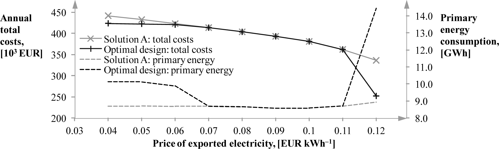
One of the most important input parameters for the plant economy is the price of exported electricity. In Figure 5, the sensitivity of ATC and PEC to the electricity price change is shown for the case where only ATC are minimized. In the range of electricity prices from 0.07 to 0.11 EUR kWh⁻¹, Solution A remains optimal. For the prices from 0.04 to 0.06 EUR kWh⁻¹, the solution with one CG of the lowest capacity and one CH is optimal. If the price is 0.12 EUR kWh⁻¹ or greater, the optimal solution has two CGs of the highest capacities and no CHs. Only in this scenario is the optimal operation regime the one where the rejection of useful heat into the environment is foreseen following the strategy to produce as much electricity as possible and sell it at a high price. Otherwise, no excess heat is produced.

5.2. Metaheuristic Methods Comparison

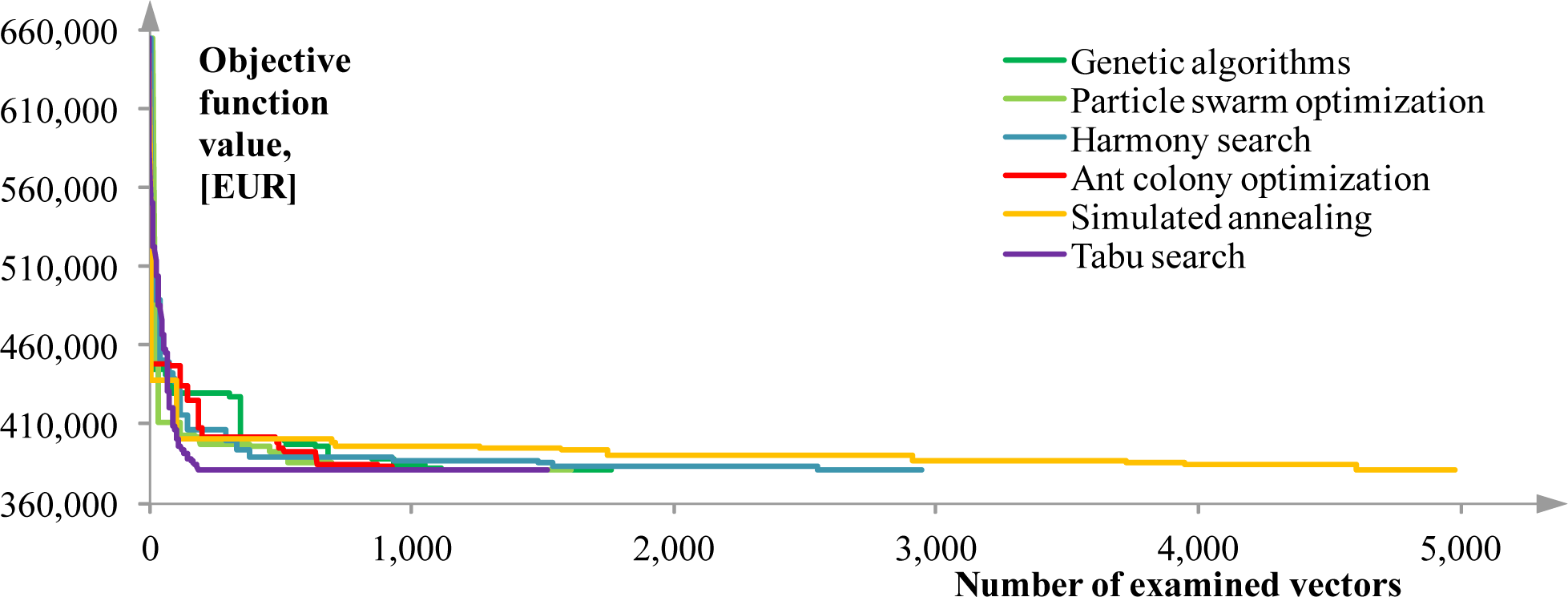
All of the exploited MH methods, except TBS, are stochastic, and it is expected that they sometimes result in solutions worse than the ones from Figure 3. This, as well as the efficiency of the MH methods, significantly depends on the adjustment of their parameters. Unfortunately, for many MH methods, there are no straightforward rules on how to set these parameters. There are some suggestions, but finally, the user has to make the decision for each problem, based on experience and multiple trial attempts. From this point of view, the methods, such as TBS, PSO or SAN, have the advantage, because they require fewer inputs. The best sets of input parameters, found after extensive testing, in terms of the quality of the solution, that provide satisfying efficiency at the same time, are shown in

Table 5. Input parameters used for metaheuristic methods comparison. GNA, genetic algorithm; PSO, article swarm optimization; ACO, ant colony optimization; SAN, simulated annealing; HMS, harmony search; TBS, tabu search.

GNA	PSO	ACO	SAN	HMS	TBS
Population size:	Swarm size:	Ants count:	Cycles count:	Memory size:	Tabu duration:
100	140	200	220	10	200
Selection method:	Min. inertia weight:	Initial trail:	Initial temperature:	Adjusting rate:
Elite	0.55	1.00	200,000.00	0.10–0.50
Mutation rate:		Decay factor:	Reduction factor:	Considering rate:
0.80		0.50	0.975	0.95
Crossover rate:		Deposit factor:
0.80		1.00
Rand.selection rate:		Importance degree:
0.05		1.00

. The results from

Table 6. Objective function values, in (EUR), for each metaheuristic method.

Run No.	GNA	PSO	ACO	SAN	HMS	TBS
1	381,068	381,418	381,068	381,068	381,068	381,068
2	381,068	381,068	384,007	381,068	384,007	381,068
3	381,068	381,068	382,081	381,068	381,068	381,068
4	381,068	381,418	381,068	381,068	381,068	381,068
5	381,068	381,068	381,068	381,068	382,431	381,068
6	384,007	381,068	381,068	381,068	381,068	381,068
7	381,068	381,068	381,068	381,068	382,431	381,068
8	381,068	381,418	384,007	381,068	381,068	381,068
9	381,068	381,068	381,068	381,418	381,068	381,068
10	381,068	381,068	381,418	381,068	384,007	381,068

correspond to 10 observed runs of each method with the parameters from Table 5 when minimizing ATC without PEC-related constraints (Solution A is optimal). The initial vector always has the largest values allowed. Convergence towards minimal ATC for this case is illustrated in Figure 6.

In addition to the reliability comparison from Table 6,

Table 7. Comparison of the applied approaches and methods.

Method	Time			Objective Function
	Exact Solution Finding	Task Completion	Relative	Value, (EUR)	Error
GNA, slower	1,251 s	1,846 s	43.5%	381,068	0.00%
GNA, quicker	108 s	358 s	8.4%	381,068	0.00%
PSO, slower	653 s	1080 s	25.5%	381,068	0.00%
PSO, quicker	259 s	350 s	8.3%	381,068	0.00%
HMS, slower	2,215 s	2,594 s	61.2%	381,068	0.00%
HMS, quicker	–	549 s	12.9%	384,007	0.77%
ACO, slower	914 s	954 s	22.5%	381,068	0.00%
ACO, quicker	–	228 s	5.4%	383,579	0.66%
SAN, slower	4,502 s	4,822 s	113.7%	381,068	0.00%
SAN, quicker	–	518 s	12.2%	384,007	0.77%
TBS, slower	1,262 s	1,372 s	32.3%	381,068	0.09%
TBS, quicker	–	790 s	18.6%	381,418	0.00%
MILP, full problem	1,278 s (0.81%)	4,242 s	100.0%	381,068	0.00%
MILP, with start values	1,240 s (0.36%)	2,975 s	70.1%	381,068	0.00%
MILP, reduced problem A	853 s (0.52%)	3,508 s	82.7%	381,068	0.00%
MILP, reduced problem B	126 s (0.58%)	1,900 s	44.8%	381,068	0.00%

illustrates the efficiency comparison of the MH methods. For each method, a slower, but more reliable, and a quicker variant are observed. The slower variants have parameters from Table 6, while parameter adjustment for the quicker ones enabled a faster completion of the optimization task: in less than 10 min. All of the tests were performed on a computer with a 64-bit operating system, 8 GB RAM and an Intel i7-4710HQ processor with 2.5 GHz, four cores and eight threads. The MILP solver used is the Gurobi Optimizer, version 6.0.

GNA and SAN were the most reliable at finding the exact solution. Although SAN is slow, its efficiency might be improved with nonlinear temperature reduction. PSO and ACO appeared faster, but sometimes tended to converge slightly prematurely to very good sub-optimal solutions. Their precision is satisfying. PSO’s premature convergence is mostly related to the binary variables. TBS always found the best solution. However, this method is not stochastic (at least not the implementation used in this research), and since the initial vector was always the same, it followed the same path in each run.

5.3. Comparison to the Superstructure-Based Approach

The illustrated approach based on the structural decomposition and MH methods is compared to the alternative and widely-used approach based on the plant superstructure. The described software solution is used to define the MILP problem that integrates synthesis, design and operation optimization. All considered plant components are included in the superstructure. The goal is to determine the models and the number of components that will be included in the plant final structure and design. This problem is similar to the original. The only difference is in the values of the RS size. Five discrete values are offered and constrained to be less than or equal to 90% of the TS size. The objective used for the comparison is ATC.

It could be problematic to define an MO problem like the one considered in this paper, since different levels of optimization might have conflicting objectives; here, the operation regimes are always cost optimal, not taking into account PEC, while synthesis and design optimization tends to minimize PEC.

The superstructure-based problem is solved with the same resources as the original one.

The results are given in Table 7. The percentages in parentheses represent the largest possible gaps from the optimum estimated when the solutions are found. Both approaches found the same optimal solution. Since this solution was found with the superstructure-based approach and MILP, it is verified as exact. The superstructure-based approach needed more time to complete the optimization task.

For the purpose of comparison, the full MILP problem was relaxed bythe operation-related binary variables, as well as part-load performance, lower bounds on the equipment load and start-up and shutdown correction considerations. This problem was solved within 4 s, yielding the sub-optimal solution that has CG model M2, one CH and other synthesis/design values the same as the optimal ones.

5.4. Combining Decomposition- and Superstructure-Based Approaches

The decomposition-based approach might also be very useful as a pre-solving concept. Other results from Table 7 represent how a combination of the two approaches might be beneficial.

First, the MILP solver found the solution of the superstructure problem 29.9% faster (in 2,975 s) when the start values of the synthesis/design variables were predefined. This is because the early determination of good feasible solutions is an important part of the branch-and-bound and branch-and-cut algorithms from the efficiency point of view. MH methods are convenient to quickly find these values. Linear relaxation might be used here, as well, but it can result in an infeasible solution, since the problems are not equivalent.

Second, the large set of good and feasible solutions quickly obtained using MH methods can be used to derive some conclusions and preselect candidate solutions, i.e., eliminate some options, reduce the problem superstructure and shrink the search space of MILP problems. From the set of vectors examined using the MH methods, it is concluded that the solutions with one CG, smaller AR models and larger TS are favorable, as well as that the ones with one CT model M1 are always better than the alternatives. Thus, the reduced Problem A is limited to the combinations with one CG, AR models M0, M1 and M2, one CT M1 and TS models M2, M3 and M4. This MILP problem is solved in 3,508 s or 17.3% faster than the full problem. Further simplification leads to the reduced Problem B, limited to one CG and models M2, M3 and M4, a maximum of two CHs, one CR, one CT M1, the largest TS and the two largest RS. It is solved in 1,900 s or 55.2% faster than the full problem.

6. Conclusions

This paper presents an approach to optimize buildings’ trigeneration energy supply plants and represents an extension of the previous work of the authors. It might be extended to other plant types.

The approach is based on the structural decomposition of the optimization problem into the synthesis and design optimization problem and the operation optimization problem. The first one is combinatorial and solved with six different metaheuristic methods: genetic algorithms, particle swarm optimization, ant colony optimization, simulated annealing, harmony search and tabu search. The second one is a mixed integer linear programming problem solved with the branch-and-cut method. These two problems are nested: whenever the objective function value is calculated for a given set of the synthesis and design variables, the operation optimization problem is constructed and solved to determine the optimal operation regime. The construction of the operation optimization problem for each candidate solution is not computationally intensive, but provides flexibility in mathematical modeling and the opportunity for operation optimization problem reduction.

This approach was applied to optimize a trigeneration plant that could be used to supply a real residential settlement in Niš, Serbia, with the objective of minimizing both the annual total costs and the primary energy consumption of the plant. The same result, shown as the Pareto curve, is obtained using each of the methods examined.

An alternative approach, based on the plant superstructure, is also used. It defines the integrated synthesis, design and operation optimization problem and solves it using the branch-and-cut method. It is used to minimize the annual total costs of the same plant and found the same optimal solution as the approach based on the structural decomposition and metaheuristics.

The approach that uses the structural decomposition and metaheuristics was faster, but sometimes near-optimal solutions were found instead of the optimal ones. It is more flexible, easier to implement and more convenient for complex or large problems. On the other hand, the superstructure-based approach that uses mixed integer linear programming is more efficient and convenient for smaller and simpler problems. It always finds the exact solution (if any), while the error gap (if allowed) might be controlled.

In addition to being faster, but reliable enough, the approach based on the structural decomposition appeared to be convenient as a part of the pre-solving process in the frame of the superstructure-based approach. The approaches were combined in two ways. In the first case, the solution found quickly with metaheuristics is used to define the starting values of the variables for the superstructure-based problem. In the second case, the superstructure is reduced using the conclusions derived from the large set of good candidate solutions obtained with metaheuristics. Consequently, the optimization problem became smaller and easier to solve. In both cases, a significant solving time reduction is achieved, compared to the full superstructure-based MILP problem.

The main focus of further work will be the exploitation of the flexibility this approach offers in the process of energy system design, especially to consider different design-related soft constraints. Furthermore, using moving-horizon short-term operation optimization [10], instead of typical periods, although computationally more intensive, might be beneficial, because it does not require one to choose typical periods, which is a critical process from the accuracy aspect, and allows the consideration of an entire horizon.

References

- EDUCOGEN—The European Educational Tool on Cogeneration; The European Association for the Promotion of Cogeneration: Brussels, Belgium, 2001.
- Frangopoulos, C.A.; von Spakovsky, M.R.; Sciubba, E. Brief Review of Methods for the Design and Synthesis Optimization of Energy Systems. Int. J. Appl. Thermodyn. 2002, 5, 151–160. [Google Scholar]
- Piacentino, A.; Cardona, E. EABOT—Energetic analysis as a basis for robust optimization of trigeneration systems by linear programming. Energy Convers. Manag. 2008, 49, 3006–3016. [Google Scholar]
- Orlando, J.A. Cogeneration Design Guide; ASHRAE: Atlanta, GA, USA, 1996. [Google Scholar]
- Oh, S.-D.; Lee, H.-J.; Jung, J.-Y.; Kwak, H.-Y. Optimal planning and economic evaluation of cogeneration system. Energy 2007, 32, 760–771. [Google Scholar]
- Buoro, D.; Pinamonti, P.; Reini, M. Optimization of a Distributed Cogeneration System with solar district heating. Appl. Energy 2014, 124, 298–308. [Google Scholar]
- Ortiga, J.; Bruno, J.C.; Coronas, A. Selection of typical days for the characterisation of energy demand in cogeneration and trigeneration optimisation models for buildings. Energy Convers. Manag. 2011, 52, 1934–1942. [Google Scholar]
- Fazlollahi, S.; Bungener, S.L.; Mandel, P.; Becker, G.; Maréchal, F. Multi-objectives, multi-period optimization of district energy systems: I. Selection of typical operating periods. Comput. Chem. Eng. 2014, 65, 54–66. [Google Scholar]
- Rieder, A.; Christidis, A.; Tsatsaronis, G. Multi criteria dynamic design optimization of a small scale distributed energy system. Energy 2014, 74, 230–239. [Google Scholar]
- Stojiljković, M.M.; Ignjatović, M.G.; Vučković, G.D. Greenhouse gasses emission assessment in residential sector through buildings simulations and operation optimization, Proceedings of the 1st South East Europe Conference on Sustainable Development of Energy, Water and Environment Systems, Ohrid, Macedonia, 29 June–4 July 2014; pp. 0134.1–0134.15.
- Ommen, T.; Markussen, W.B.; Elmegaard, B. Comparison of linear, mixed integer and non-linear programming methods in energy system dispatch modelling. Energy 2014, 74, 109–118. [Google Scholar]
- Pruitt, K.A.; Braun, R.J.; Newman, A.M. Evaluating shortfalls in mixed-integer programming approaches for the optimal design and dispatch of distributed generation systems. Appl. Energy 2013, 102, 386–398. [Google Scholar]
- Aki, H.; Oyama, T.; Tsuji, K. Analysis of energy service systems in urban areas and their CO2 mitigations and economic impacts. Appl. Energy 2006, 83, 1076–1088. [Google Scholar]
- Magnani, F.S.; da Silva, P.P.; Guerra, M.R.; Hornsby, E.M. Adaptability of optimized cogeneration systems to deal with financial changes occurring after the design period. Energy Build. 2013, 58, 183–193. [Google Scholar]
- Petruschke, P.; Gasparovic, G.; Voll, P.; Krajačić, G.; Duić, N.; Bardow, A. A hybrid approach for the efficient synthesis of renewable energy systems. Appl. Energy 2014, 135, 625–633. [Google Scholar]
- Dvořák, M.; Havel, P. Combined heat and power production planning under liberalized market conditions. Appl. Therm. Eng. 2012, 43, 163–173. [Google Scholar]
- Rao, S.S. Engineering Optimization: Theory and Practice; John Wiley & Sons, Inc.: Hoboken, NJ, USA, 2009. [Google Scholar]
- Ferrari-Trecate, G.; Gallestey, E.; Letizia, P.; Spedicato, M.; Morari, M.; Antoine, M. Modeling and Control of Co-Generation Power Plants: A Hybrid System Approach; Technical Report AUT01-18; ETH Zürich, Automatic Control Laboratory: Zürich, Switzerland, 2002. [Google Scholar]
- Lozano, M.A.; Ramos, J.C.; Carvalho, M.; Serra, L.M. Structure optimization of energy supply systems in tertiary sector buildings. Energy Build. 2009, 41, 1063–1075. [Google Scholar]
- Lozano, M.A.; Ramos, J.C.; Serra, L.M. Cost optimization of the design of CHCP (combined heat, cooling and power) systems under legal constraints. Energy 2010, 35, 794–805. [Google Scholar]
- Casisi, M.; Pinamonti, P.; Reini, M. Optimal lay-out and operation of combined heat & power (CHP) distributed generation systems. Energy 2009, 34, 2175–2183. [Google Scholar]
- Seo, H.; Sung, J.; Oh, S.-D.; Oh, H.-S.; Kwak, H.-Y. Economic optimization of a cogeneration system for apartment houses in Korea. Energy Build. 2008, 40, 961–967. [Google Scholar]
- Arcuri, P.; Florio, G.; Fragiacomo, P. A mixed integer programming model for optimal design of trigeneration in a hospital complex. Energy 2007, 32, 1430–1447. [Google Scholar]
- Wakui, T.; Yokoyama, R. Optimal sizing of residential SOFC cogeneration system for power interchange operation in housing complex from energy-saving viewpoint. Energy 2012, 41, 65–74. [Google Scholar]
- Wakui, T.; Yokoyama, R. Optimal structural design of residential cogeneration systems in consideration of their operating restrictions. Energy 2014, 64, 719–733. [Google Scholar]
- Steen, D.; Stadler, M.; Cardoso, G.; Groissböck, M.; DeForest, N.; Marnay, C. Modeling of thermal storage systems in MILP distributed energy resource models. Appl. Energy 2015, 137, 782–792. [Google Scholar]
- Piacentino, A.; Barbaro, C.; Cardona, F.; Gallea, R.; Cardona, E. A comprehensive tool for efficient design and operation of polygeneration-based energy µgrids serving a cluster of buildings. Part I: Description of the method. Appl. Energy 2013, 111, 1204–1221. [Google Scholar]
- Piacentino, A.; Barbaro, C. A comprehensive tool for efficient design and operation of polygeneration-based energy µgrids serving a cluster of buildings. Part II: Analysis of the applicative potential. Appl. Energy 2013, 111, 1222–1238. [Google Scholar]
- Mehleri, E.D.; Sarimveis, H.; Markatos, N.C.; Papageorgiou, L.G. Optimal design and operation of distributed energy systems: Application to Greek residential sector. Renew. Energy 2013, 51, 331–342. [Google Scholar]
- Liu, P.; Georgiadis, M.C.; Pistikopoulos, E.N. An energy systems engineering approach for the design andoperation of microgrids in residential applications. Chem. Eng. Res. Des. 2013, 91, 2054–2069. [Google Scholar]
- Liang, H.; Zhuang, W. Stochastic Modeling and Optimization in a Microgrid: A Survey. Energies 2014, 7, 2027–2050. [Google Scholar]
- Bracco, S.; Dentici, G.; Siri, S. Economic and environmental optimization model for the design and the operation of a combined heat and power distributed generation system in an urban area. Energy 2013, 55, 1014–1024. [Google Scholar]
- Menon, R.P.; Paolone, M.; Maréchal, F. Study of optimal design of polygeneration systems in optimal control strategies. Energy 2013, 55, 134–141. [Google Scholar]
- Piacentino, A.; Cardona, E. On thermoeconomics of energy systems at variable load conditions: Integrated optimization of plant design and operation. Energy Convers. Manag. 2007, 48, 2341–2355. [Google Scholar]
- Li, H.; Nalim, R.; Haldi, P.-A. Thermal-economic optimization of a distributed multi-generation energy system—A case study of Beijing. Appl. Therm. Eng. 2006, 26, 709–719. [Google Scholar]
- Burer, M.; Tanaka, K.; Favrat, D.; Yamada, K. Multi-criteria optimization of a district cogeneration plant integrating a solid oxide fuel cell-gas turbine combined cycle, heat pumps and chillers. Energy 2003, 28, 497–518. [Google Scholar]
- Weber, C.; Maréchal, F.; Favrat, D.; Kraines, S. Optimization of an SOFC-based decentralized polygeneration system for providing energy services in an office-building in Tokyo. Appl. Therm. Eng. 2006, 26, 1409–1419. [Google Scholar]
- Moradi, M.H.; Hajinazari, M.; Jamasb, S.; Paripour, M. An energy management system (EMS) strategy for combined heat and power (CHP) systems based on a hybrid optimization method employing fuzzy programming. Energy 2013, 49, 86–101. [Google Scholar]
- Fazlollahi, S.; Mandel, P.; Becker, G.; Maréchal, F. Methods for multi-objective investment and operating optimization of complex energy systems. Energy 2012, 45, 12–22. [Google Scholar]
- Gholamhossein, Abdollahi. H.S. Application of the multi-objective optimization and risk analysis for the sizing of a residential small-scale CCHP system. Energy Build. 2013, 60, 330–344. [Google Scholar]
- Barbato, A.; Capone, A. Optimization Models and methods for demand-side management of residential users: A survey. Energies 2014, 7, 5787–5824. [Google Scholar]
- Stojiljković, M.M.; Stojiljković, M.M.; Blagojević, B.D. Optimization of trigeneration Systems: A combinatorial metaheuristic approach, Proceedings of the 16th Symposium on Thermal Science and Engineering of Serbia, Sokobanja, Serbia, 22–25 October 2013; University of Niš, Faculty of Mechanical Engineering in Niš: Crveni Krst, Niš, Serbia, 2013; pp. 601–615.
- EnergyPlus Energy Simulation Software. Weather Data, Available online: http://apps1.eere.energy.gov/buildings/energyplus/weatherdata/6_europe_wmo_region_6/SRB_Belgrade.132720_IWEC.zip accessed on 6 December 2014.
- Stojiljković, M.M.; Blagojević, B.D.; Vučković, G.D.; Ignjatović, M.G.; Mitrović, D.M. Optimization of operation of energy supply systems with co-generation and absorption refrigeration. Therm. Sci. 2012, 16, 409–422. [Google Scholar]
- Sakawa, M.; Kato, K.; Ushiro, S. Operational planning of district heating and cooling plants through genetic algorithms for mixed 0–1 linear programming. Eur. J. Oper. Res. 2002, 137, 677–687. [Google Scholar]
- Bejan, A.; Tsatsaronis, G.; Moran, M. Thermal Design and Optimization; John Wiley & Sons Inc.: New York, NY, USA, 1996. [Google Scholar]
- Cardona, E.; Sannino, P.; Piacentino, A.; Cardona, F. Energy saving in airports by trigeneration. Part II: Short and long term planning for the Malpensa 2000 CHCP plant. Appl. Therm. Eng. 2006, 26, 1437–1447. [Google Scholar]
- Frangopoulos, C.A.; Dimopoulos, G.G. Effect of reliability considerations on the optimal synthesis, design and operation of a cogeneration system. Energy 2004, 29, 309–329. [Google Scholar]
- Jarboui, B.; Damak, N.; Siarry, P.; Rebai, A. A combinatorial particle swarm optimization for solving multi-mode resource-constrained project scheduling problems. Appl. Math. Comput. 2008, 195, 299–308. [Google Scholar]
- Tchomté, S.K.; Gourgand, M. Particle swarm optimization: A study of particle displacement for solving continuous and combinatorial optimization problems. Int. J. Prod. Econ. 2009, 121, 57–67. [Google Scholar]
- Mavrotas, G.; Diakoulaki, D.; Florios, K.; Georgiou, P. A mathematical programming framework for energy planning in services’ sector buildings under uncertainty in load demand: The case of a hospital in Athens. Energy Policy 2008, 36, 2415–2429. [Google Scholar]
- Gurobi Optimizer, Version 6.0, Available online: http://www.gurobi.com accessed on 6 December 2014.
- Microsoft Solver Foundation, Version 3.1, Available online: http://msdn.microsoft.com/en-us/devlabs/hh145003.aspx accessed on 6 December 2014.
- LP Solve, Version 5.5.2.0, Available online: http://sourceforge.net/projects/lpsolve/ accessed on 6 December 2014.
- Grekas, D.N.; Frangopoulos, C.A. Automatic synthesis of mathematical models using graph theory for optimisation of thermal energy systems. Energy Convers. Manag. 2007, 48, 2818–2826. [Google Scholar]