Article

Numerical and Theoretical Investigations Concerning the Continuous-Surface-Curvature Effect in Compressor Blades

1
Key Laboratory for Thermal Science and Power Engineering of Ministry of Education, Department of Thermal Engineering, Tsinghua University, Beijing 100084, China
2
Collaborative Innovation Center of Advanced Aero-Engine, Beijing 100191, China
*
Author to whom correspondence should be addressed.
Energies 2014, 7(12), 8150-8177; https://doi.org/10.3390/en7128150
Submission received: 3 October 2014 / Revised: 24 November 2014 / Accepted: 27 November 2014 / Published: 9 December 2014

Abstract

:
Though the importance of curvature continuity on compressor blade performances has been realized, there are two major questions that need to be solved, i.e., the respective effects of curvature continuity at the leading-edge blend point and the main surface, and the contradiction between the traditional theory and experimental observations in the effect of those novel leading-edge shapes with smaller curvature discontinuity and sharper nose. In this paper, an optimization method to design continuous-curvature blade profiles which deviate little from datum blades is proposed, and numerical and theoretical analysis is carried out to investigate the continuous-curvature effect on blade performances. The results show that the curvature continuity at the leading-edge blend point helps to eliminate the separation bubble, thus improving the blade performance. The main-surface curvature continuity is also beneficial, although its effects are much smaller than those of the blend-point curvature continuity. Furthermore, it is observed that there exist two factors controlling the leading-edge spike, i.e., the curvature discontinuity at the blend point which dominates at small incidences, and the nose curvature which dominates at large incidences. To the authors’ knowledge, such mechanisms have not been reported before, and they can help to solve the sharp-leading-edge paradox.

1. Introduction

The design principles and methods for blade profiles have been studied over the years to improve fan or compressor efficiency, and thus improve the overall performance of gas turbine-based power plants and aeroengines. The continuity or discontinuity of blade surface curvature is a relatively new topic in the design or optimization of blade profiles in terms of its potential effects on the surface boundary layer and thus the total pressure loss and the effective incidence range. In fact, discontinuity of surface curvature is very common in compressor blade profiles, existing either at the blend point of the conventional circular or elliptical leading edges to the main parts of the surface or within the main parts themselves, e.g., at the blend points between adjacent sections of a multi-circular arc (MCA) airfoil.
The curvature discontinuity at the blend point of a leading edge to the main surface is highly related to the leading edge shape. The traditional circular leading edge results in a large curvature discontinuity when it is blended with the main surface, which is thought to lead to a large spike in the pressure distribution on the profile and result in a narrow working range of the blade cascade. A lot of effort has been put into optimizing the circular leading edge to overcome its drawback. The most famous one is the elliptical leading edge [1,2], which has already been widely used in industry, and some other new leading-edge shapes have also been presented, e.g., [3,4]. If the above new leading-edge shapes are compared with the circular one, it is found that these new shapes with smaller curvature discontinuity have generally shown sharper nose when the main surface of the blade is fixed, which can be seen from Figure 1 and Figure 2. Unfortunately, the effect of such new sharper leading edge has not been completely understood yet and there still exists some contradiction between the present theory and the observed physical phenomena. The conventional airfoil theory suggested that a sharp leading edge usually leads to a large spike in the pressure distribution on the profile and results in a narrow working range of the blade cascade, which can be seen from the criteria for leading-edge separation proposed by Tuck [5] and Elmstrom et al. [6]. However, it has been found paradoxically in experiments and numerical computations by several researchers that instead the sharpest leading edge has the widest working range [3,7], and it has been widely accepted that the elliptical leading edge helps to avoid the separation bubble, to reduce the profile loss and to enlarge the working range [1,2,8,9,10]. Therefore, further studies are still needed to clarify the real effects of curvature continuity at the blend points and to resolve the paradox about the leading edge sharpness.
The importance of the main-part curvature of the blade has also been realized by some authors. Korakianitis [11,12,13] found that the aerodynamic and heat transfer performances of turbine cascades are affected significantly by the curvature distributions and proposed a design method for turbine blades, in which a curvature distribution of the blade is prescribed to construct a blade surface with both a continuous curvature and gradient of curvature.
Figure 1. New leading-edge shape proposed in [4].
Energies 07 08150 g001
Figure 2. Spikeless continuous-curvature leading edge in [3]: (a) circular LE; (b) elliptical LE; (c) spikeless continuous-curvature LE.
Energies 07 08150 g002
The method has been further extended to compressor blades and reduction of losses inside the boundary layer on the suction surface as well as improvement of blade performance is observed numerically for the optimized compressor blades [14]. Sommer [15] and Fathi [16] also presented surface curvature optimizations for compressor blades. It should be noted that in their research the curvature as well as the gradient of curvature of the blade surface are both continuous, since the curvature distributions are defined by Bezier splines or B-splines.
The advantages in designing a blade surface with a continuous or smooth curvature have been shown in the above results, the effects of main-part curvature continuity, nevertheless, still need further research in the following respects. Firstly, curvatures within the main surface and at the blend point of the leading edge to the main surface are optimized at the same time in the above research, and it is difficult to tell whether the improvement is induced by optimization of the leading edge or of the main surface. Secondly, in their research, optimization of the blades has led to distinctively different blade shapes, including their camber lines and thickness distributions, so it is not clear how much loss reduction is brought about by the curvature continuity itself, rather than by alteration of the blade shapes.
Hence, the objectives of this paper are to solve the abovementioned two questions concerning the effect of curvature continuity of compressor blade profiles, that is: what are the respective effects of curvature continuity at the leading-edge blend point and in the main surface; how to explain the sharp leading edge paradox. Thus, first an optimization method for designing continuous-curvature blade profiles without severe modification to datum ones will be proposed, and then the curvature effects at the blend point and in the main surface on the blade performance will be investigated numerically. Finally, theoretical analysis will be carried out to find deeper explanations for the above questions, which can also support the numerical results.

2. The Optimization Method of Continuous-Curvature Blade Profile

Unlike the optimization methods in [11,12,13,14,15,16], which aim at building a blade surface with the best aerodynamic performance and result in much alteration of the shape of blade surface, the method suggested in this paper is to get an optimized continuous curvature blade without major modification to the datum blade geometry, which helps to exclude the influence of blade shape alteration when analyzing the effect of curvature continuity. The method for the leading edge and the main surface, respectively, is detailed as follows.

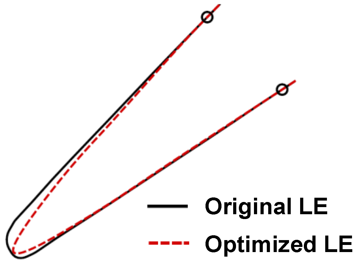
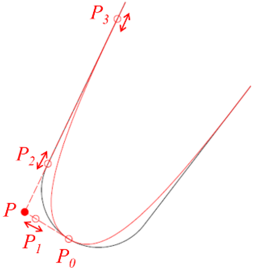
2.1. The Optimization of Leading Edge

The alternative leading-edge geometry is defined with two cubic Bezier splines, separated by the nose of the datum blade. The cubic Bezier spline is used for the characteristics of its endpoint tangent vector. As shown in Figure 3, the four control points of the upper Bezier spline are P0, P1, P2 and P3. P0 is fixed at the nose of the datum blade, and the tangent vector at P0 is fixed to the datum nose tangential direction. P3 is moveable along the suction surface of the datum blade, and the tangent vector at P3 is also determined by the datum tangential direction there. P is the intersection point of the tangent vectors at P0 and P3, then the control point P1 must be located in the line P0P, while P2 in P3P, so as to ensure the smooth transition of the profile at the nose (P0) as well as at the blend point with the main surface (P3). The coordinates of P0, P1, P2, P3 and P are denoted as (X0, Y0), (X1, Y1), (X2, Y2), (X3, Y3) and (X, Y), respectively. Two new design variables are defined to describe the locations of P1 and P2, i.e.:
ϕ 1 = ( X 1 X 0 ) / ( X X 0 )
ϕ 1 = ( X 2 X 3 ) / ( X X 3 )
Figure 3. Leading-edge geometry definition.
Energies 07 08150 g003
Then the independent design variables can be reduced to X3, ϕ1 and ϕ2. The value of design variables should ensure the curvature continuity at P3, i.e.:
| K P 3 , Leading edge K P 3 , Main surface | ε 1
The following additional constraints should also be fulfilled:
| X 3 X 0 | / C x ε 2
K 0 ε 3
Constraint Equation (3) is used to ensure the curvature continuity at the blend point, so the value of ɛ1 should be small enough. Constraint Equation (4) is used to limit the geometry variation within the leading-edge region, so that the main-part geometry of the blade surfaces will not be altered. Constraint Equation (5) is used to prevent too sharp a leading-edge geometry, the reason of which will be discussed hereinafter. In the present research, the value of ɛ1, ɛ2 and ɛ3 are chosen as 0.1, 0.05 and 20 mm−1, respectively. The design variables can be optimized to satisfy the above requirements manually or automatically with any heuristic or evolutionary-algorithm optimization method. The design method for the other half of the leading edge is the same, so it is omitted here. It should also be noted that the curvature continuity at P0 between the two halves of the leading-edge curve must be maintained.

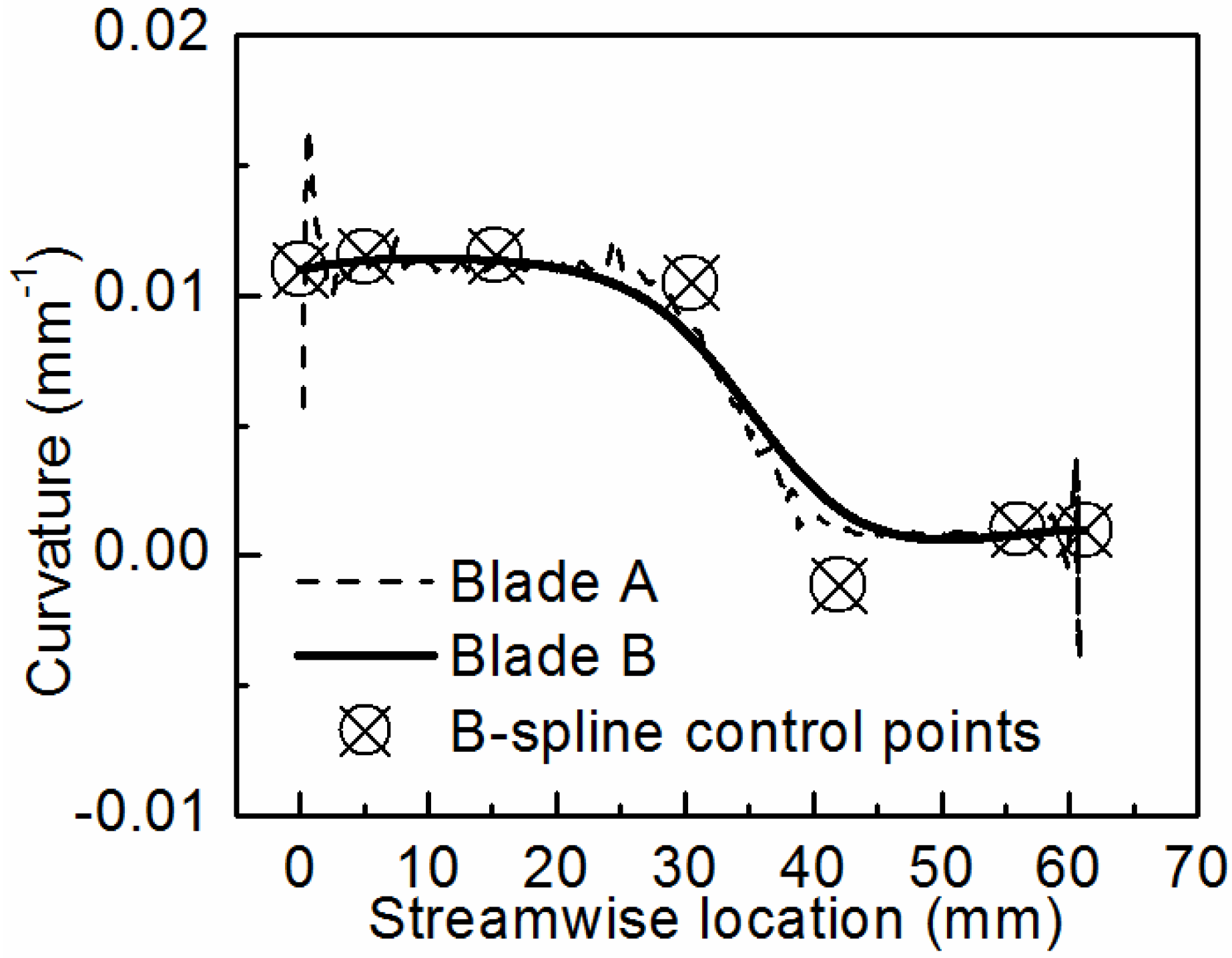
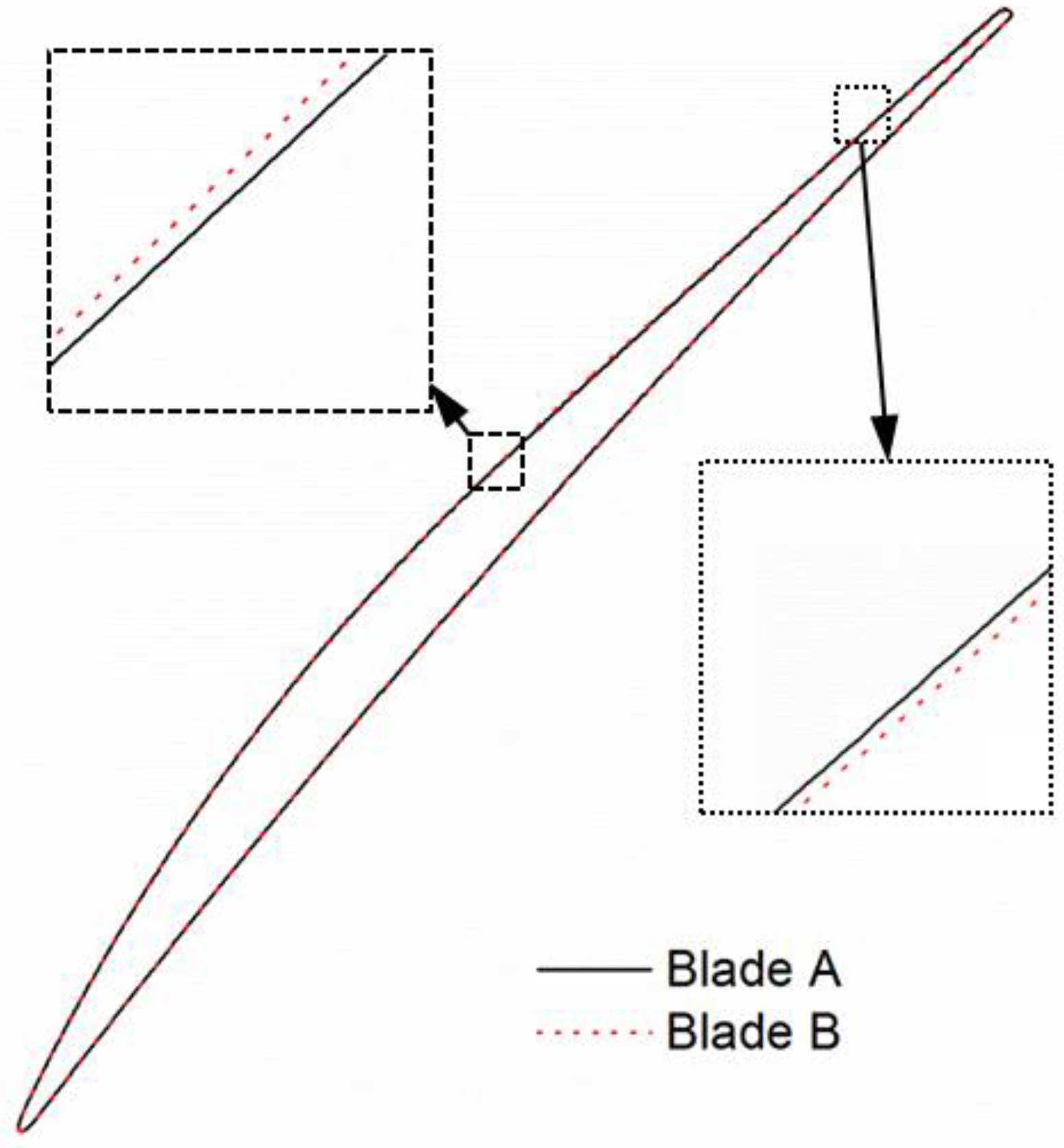
2.2. The Optimization of the Main Part of Blade Surface

In order to get a blade surface with continuous curvature, the blade surface is represented by its streamwise curvature distribution, which is specified using a cubic B-spline curve as in [15].
The streamwise curvature distribution may be described as:
[ s ( u ) K ( u ) ] = i = 0 n 1 N i , p ( u ) Q i , 0 u 1
The basis functions N i , p ( u ) are defined as:
N i , 0 ( u ) = { 1 , for u i u < u i + 1 0 , for u   at   elsewhere
N i , j ( u ) = u u i u i + j u i N i , j 1 ( u ) + u i + j + 1 u u i + j + 1 u i + 1 N i + 1 , j 1 ( u ) , j = 1 , 2 , ... , p .
A cubic B-spline curve with 7 control points is used to define the curvature distribution and calculate the blade surface. A uniform knot vector is defined as:
U = [ 0 , 0 , 0 , 0 , 0.25 , 0.5 , 0.75 , 1 , 1 , 1 , 1 ] T
The blade surface coordinates are calculated from the curvature distribution as follows. For an infinitesimal element ds of the blade surface as shown in Figure 4, the following equations can be derived:
d x = cos ( φ ) d s
d y = sin ( φ ) d s
where φ is related to the slope of the curve, φ = arctan(k). The infinitesimal element can be approximated as a circular arc, so there is:
d s = K
Those equations will be used in the following steps:
(1)
The control points Qi (si, Ki) of the cubic B-spline curve for curvature distribution are defined.
(2)
The coordinates (x0, y0) and slope k0 at the starting point of the main surface, i.e., at the blend point, are defined according to the datum blade, and the slope angle φ0 is calculated.
(3)
The streamwise distribution of curvature K(s) is discretized by Equations (6)–(9).
(4)
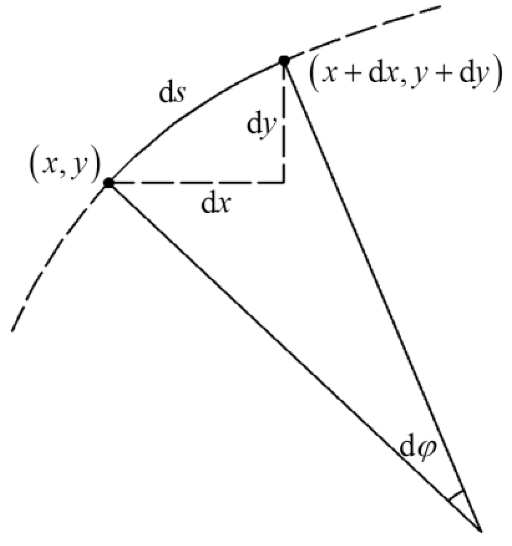
The streamwise distribution of the slope angle φ(s) is calculated by Equation (12).
(5)
The Cartesian coordinates of the new blade surface along the streamwise direction are calculated by Equations (10) and (11).
Figure 4. An infinitesimal element of the blade surface.
Energies 07 08150 g004
Thus, the obtained main surface will have a continuous curvature distribution. In order to get the optimized continuous curvature main surface without much deviation from the shape of the datum blade, a combination of Sequential Quadratic Programming method and Mixed Integer Optimization method is used to get the favorable B-spline control points, and the objective function reads as:
min [ max j ( d j ) ]
where dj represents the distance between the discrete point (xj, yj) on the optimized main surface and the datum blade surface.
The following constraints are adopted:
0 s i S ori
0 K i K max
where Sori is the streamwise length of the datum-blade main surface, and Kmax is a predefined maximum curvature to prevent the divergence of optimization process, which will not alter the final result and a value of 10 mm−1 is adopted in the present research.
Moreover, it should be noted that the optimized main surface in the present research has not only continuous curvature but also continuous gradient of curvature, since the curvature distribution is defined by the cubic B-spline curve.
After optimization of main surfaces, the trailing edge is rebuilt with the original camber length maintained. Since the trailing-edge geometry is not the focus of this research, the detailed rebuilding procedures are omitted here for simplicity.
In summary, the characteristics of the optimized blade are continuous curvature on the leading edge as well as at the blend point of the leading edge to the main surface; continuous curvature and gradient of curvature distributions in the main surfaces deviating little from the datum profile.

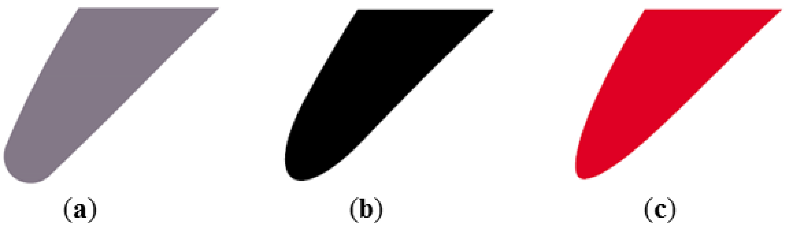
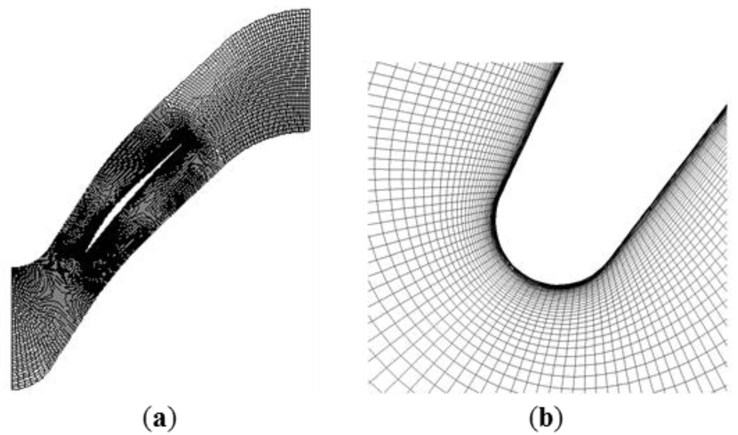
3. Objects and Numerical Methods

In the present study, an industrial compressor blade profile will be optimized by using the above methods. The performances of the datum and optimized blade profiles will be computed and compared to show the effects of surface curvature continuity. The geometry of the blade is shown in Figure 5. The inlet total pressure is 1.644 × 10⁶ Pa, the total temperature is 632.33 K, and the outlet static pressure is 1.610 × 10⁶ Pa, corresponding to the actual working condition with a Reynolds number around 106. The inlet turbulence intensity is 5% and the viscosity ratio is 10.
Figure 5. Details of the studied blade profile.
Energies 07 08150 g005
A Computational Fluid Dynamics (CFD) method is used to analyze performances and flow details of the datum and optimized continuous-curvature blade, that is, the commercial code CFX based on RANS equations with k-ω SST turbulence model and the correlation-based γ-Reθ transition model is adopted. Accurate prediction of transition in the boundary layer is crucial for successful computation of compressor cascade flows. The γ-Reθ transition model has shown very good results for transitional flows in turbomachinery [17,18,19,20], and it is considered to be the state of the art [21]. More specifically, Langtry [17] validated CFX with the γ-Reθ model on computing the flowfield around a double-circular airfoil, and Korakianitis [14] used the software FLUENT with the γ-Reθ model in his curvature-based blade optimization system. Marciniak [21] validated the ability of γ-Reθ model on predicting the performance of a CDA profile. In his paper the results from the different turbulence and transition models and the experimental measurements are discussed in terms of loss coefficients and Mach number distributions, and it is found that by γ-Reθ model the computed losses are closer to the experimental values compared with MultiMode transition model and the k-ω and k-ω SST turbulence models, and the physics of the flow is also well reproduced in a wide range of flow conditions.
An HOH-type grid is used for calculations, as shown in Figure 6. The grid near the leading edge is refined to capture more flow details there, and y+ <1 is ensured at the blade surface to satisfy the requirement of the turbulence and transition models.
Figure 6. Calculation grid: (a) the whole grid; (b) the grid near the leading edge.
Energies 07 08150 g006
The grid quality is very important for modeling of transitional flows, so a grid independence test is carried out for the datum blade. The sizes of three different grids are shown in Table 1. The loss buckets of the blade calculated for the above grids are shown in Figure 7, which indicate that Grid 2 would be sufficient for the following computations.
Table 1. Sizes of different grids.
No.Total sizeSize of the O-type region
119,527309 × 57
243,307481 × 81
393,707721 × 121
Figure 7. Loss buckets calculated for different grids.
Energies 07 08150 g007

4. Numerical Investigations about the Continuous-Curvature Effect

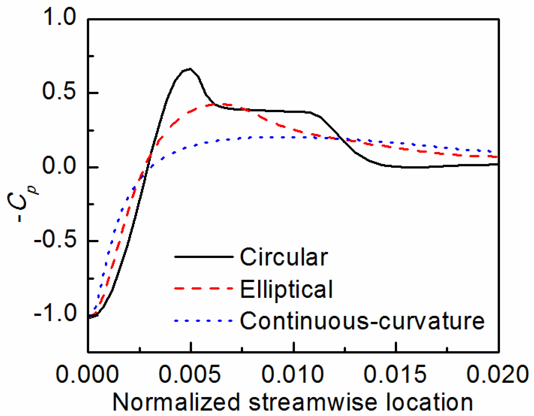
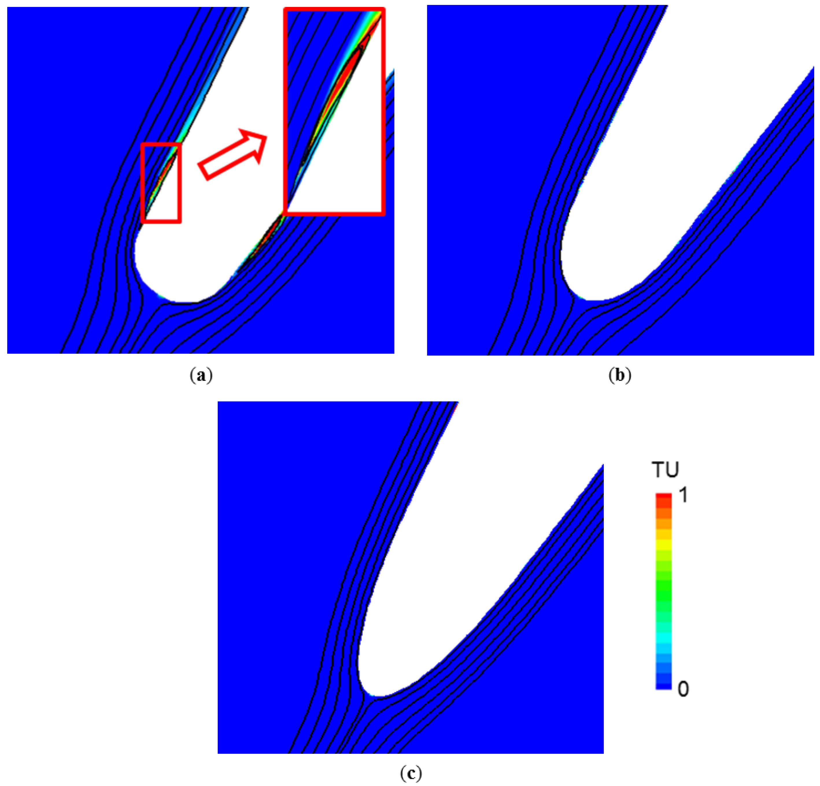
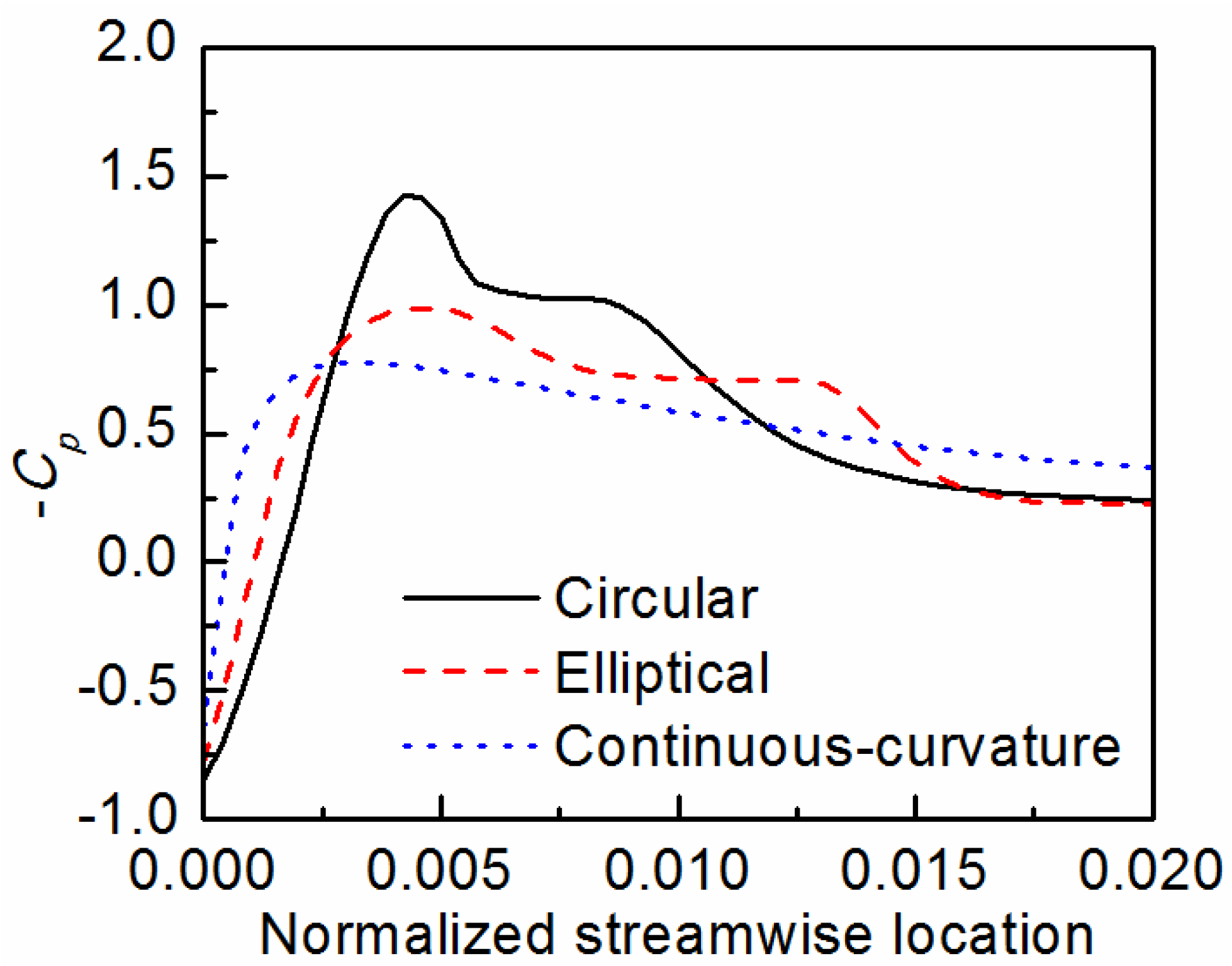
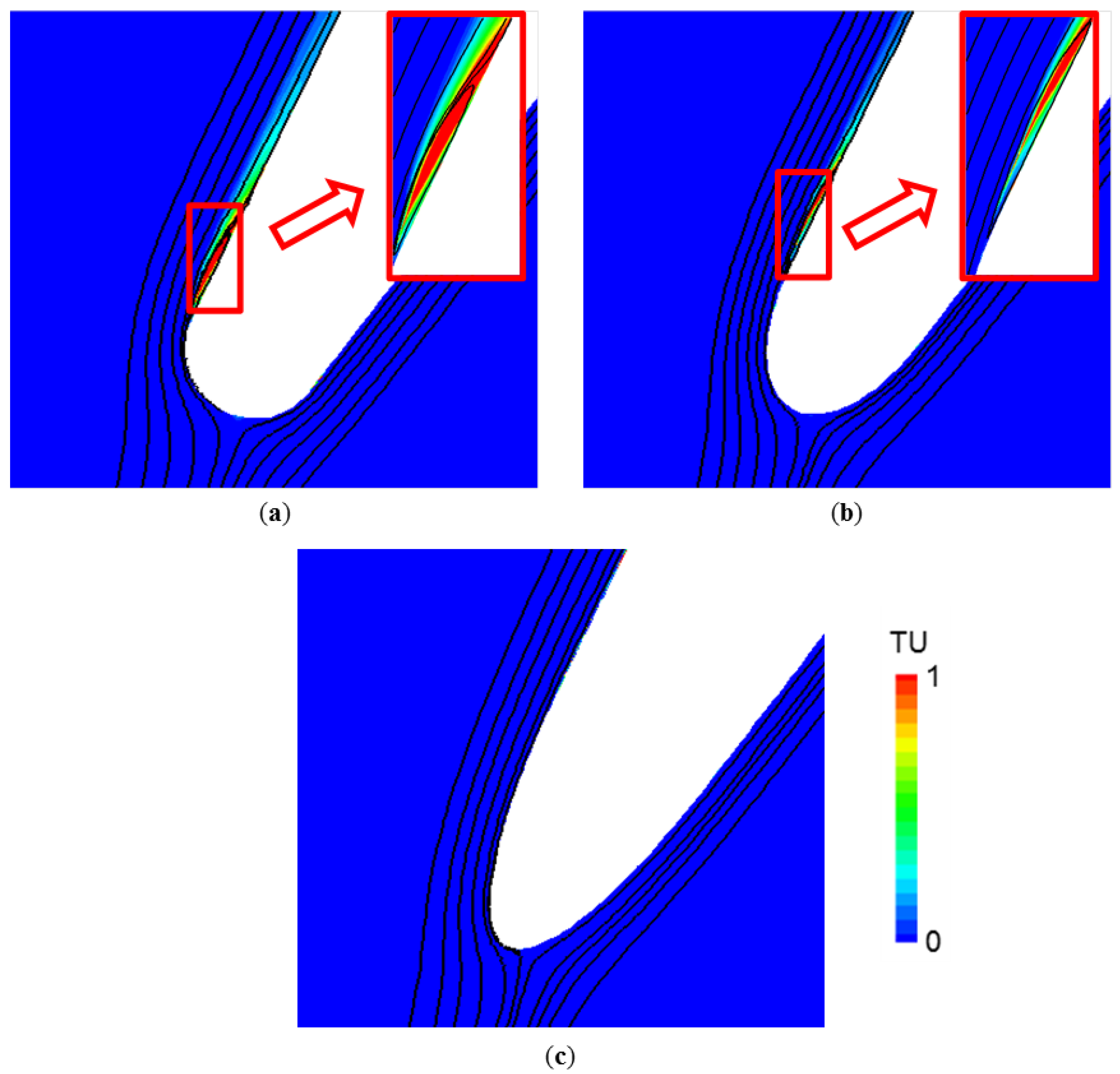
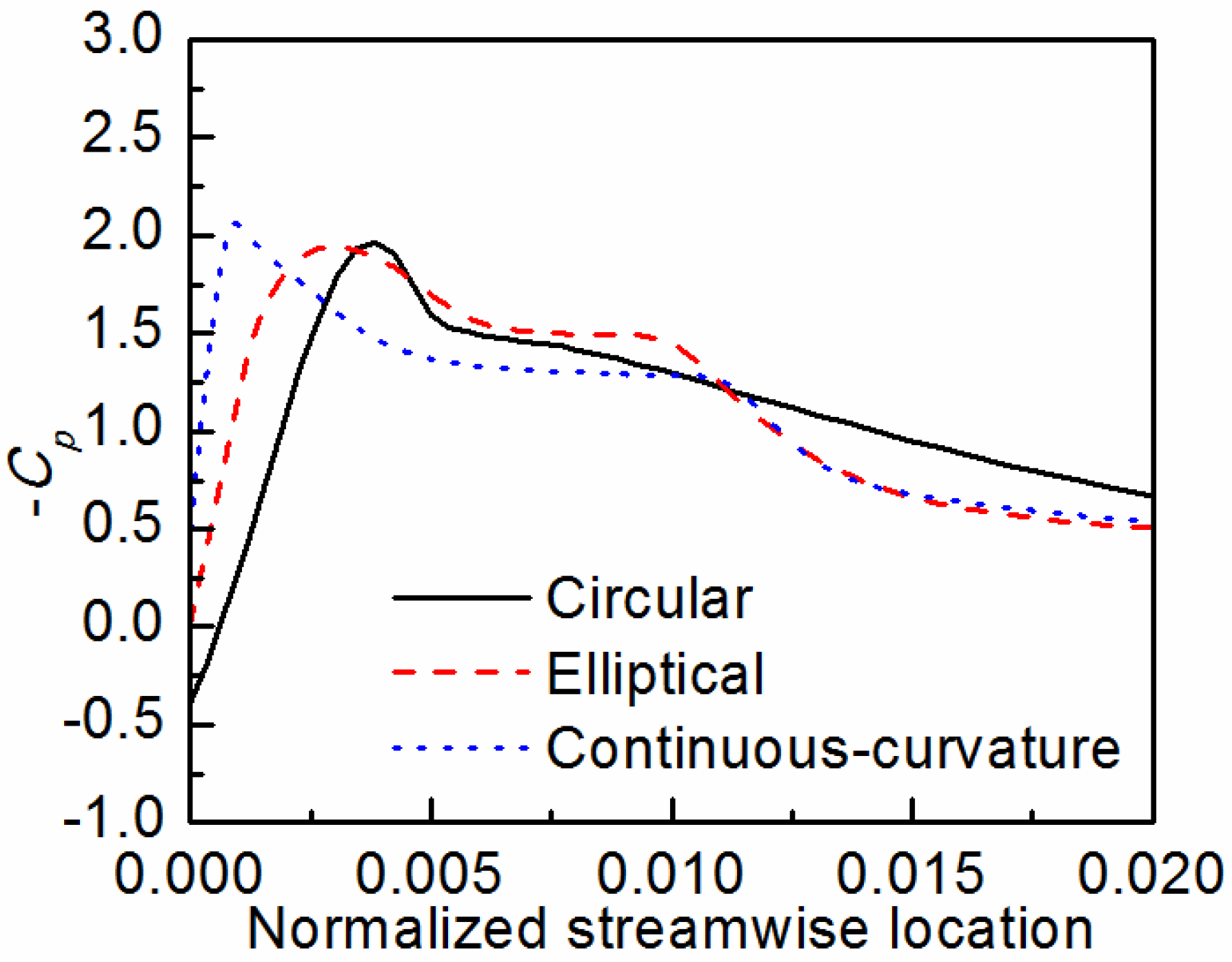
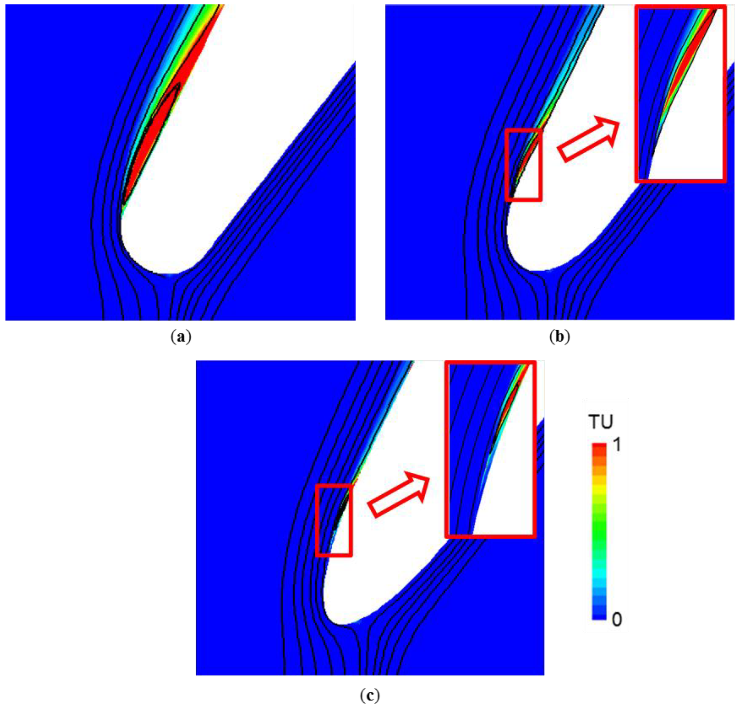
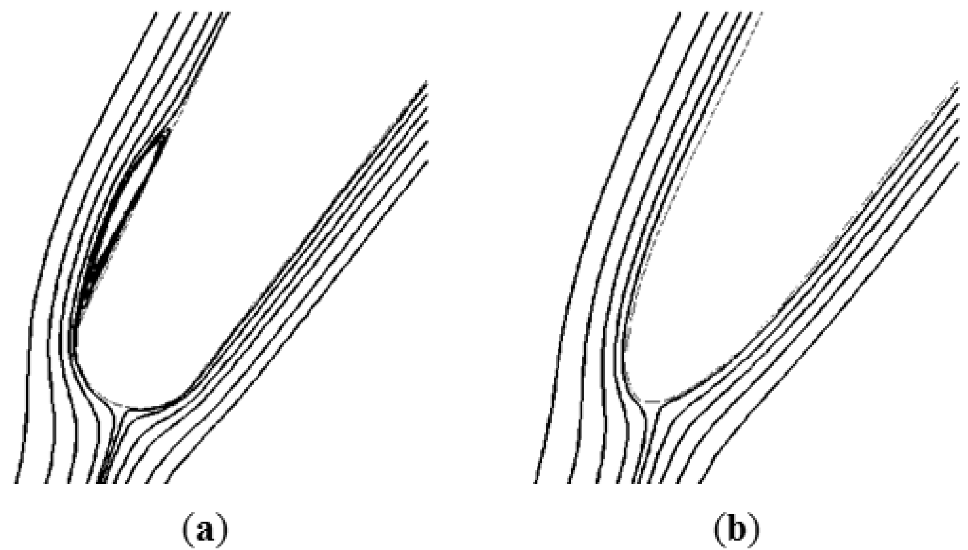
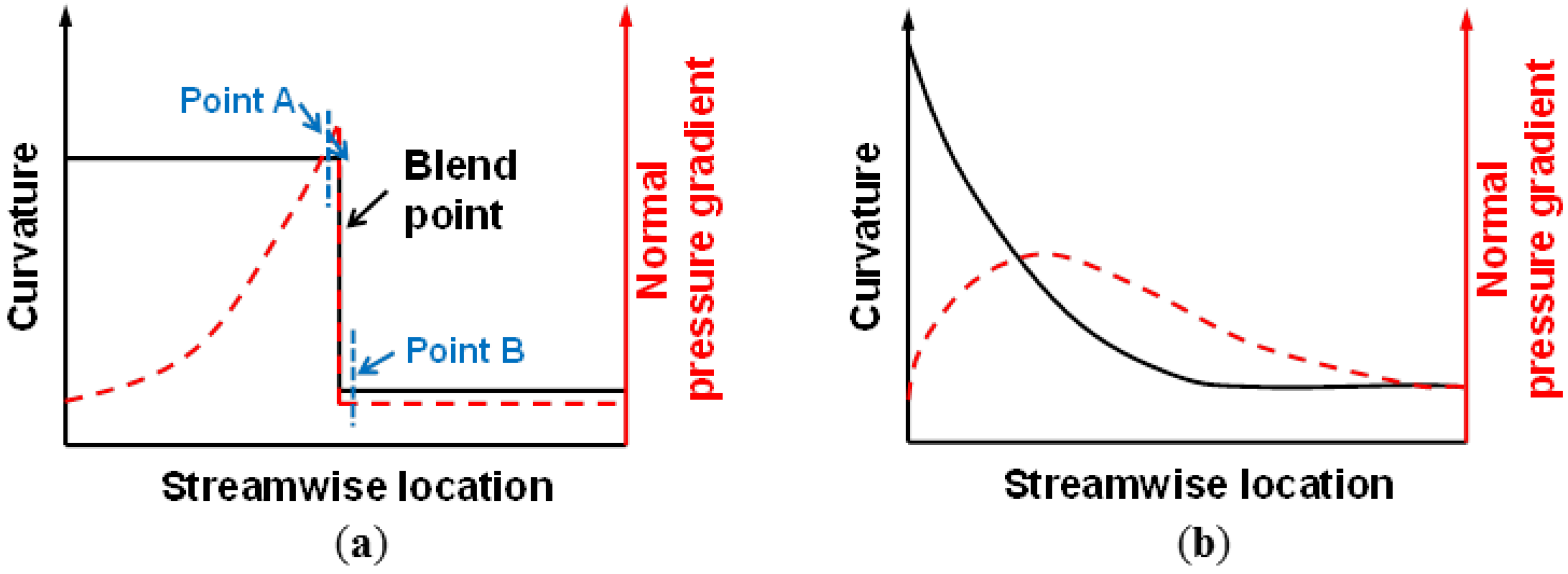
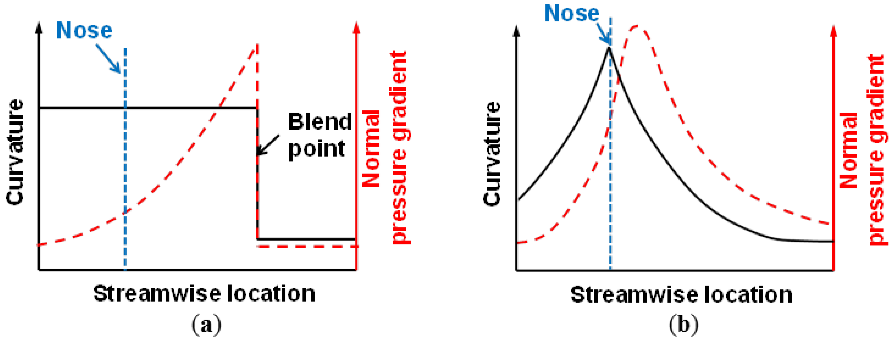
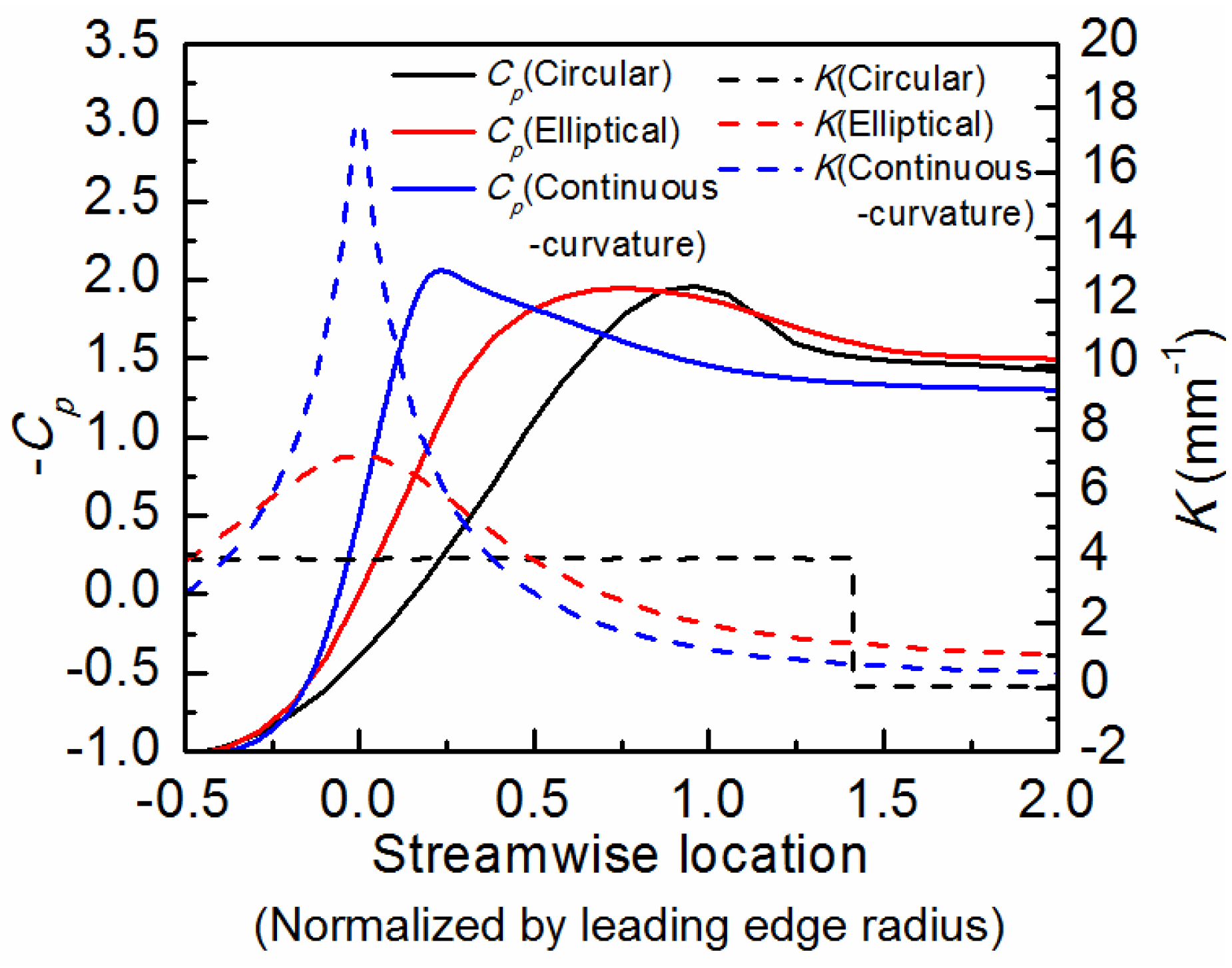
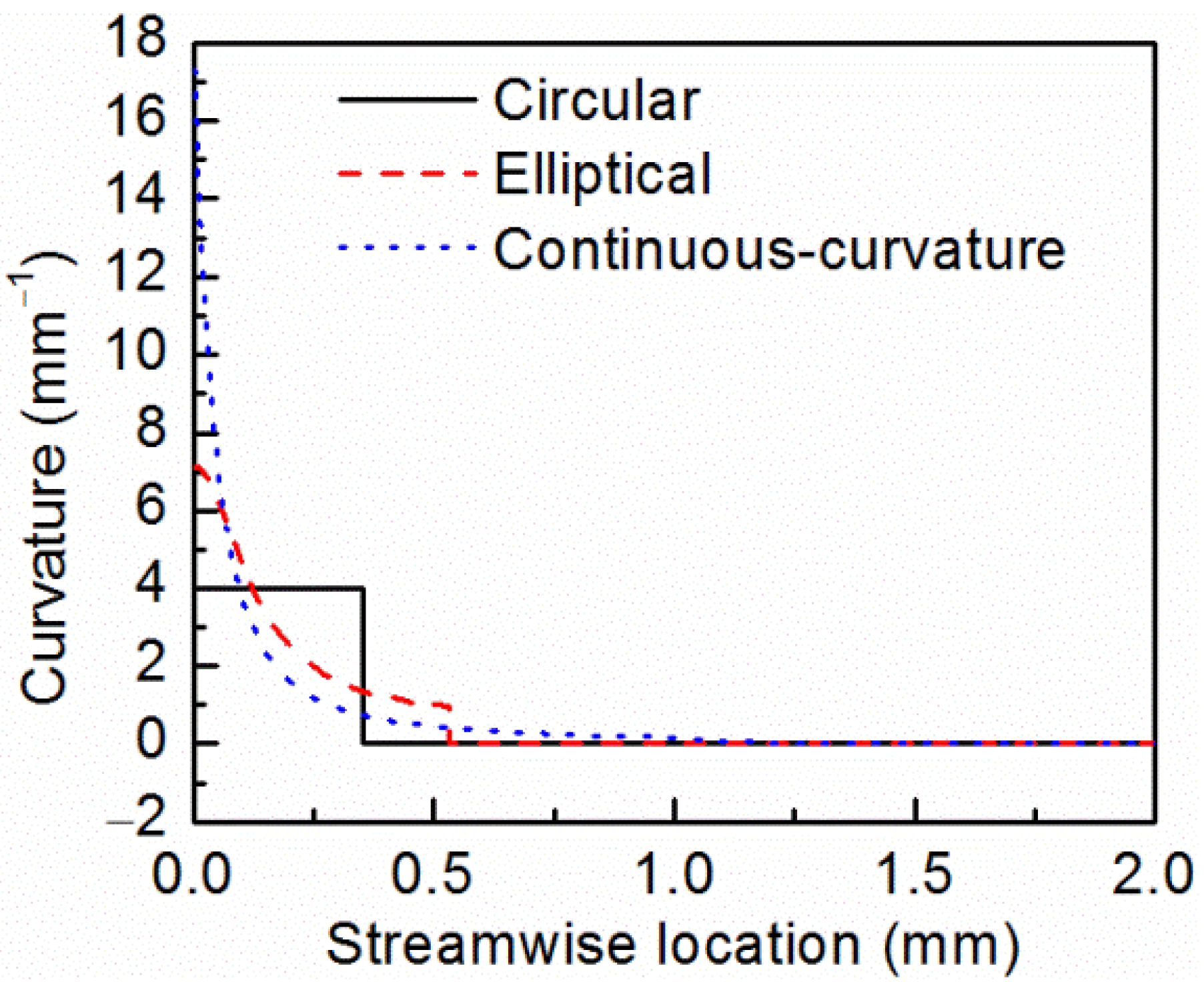
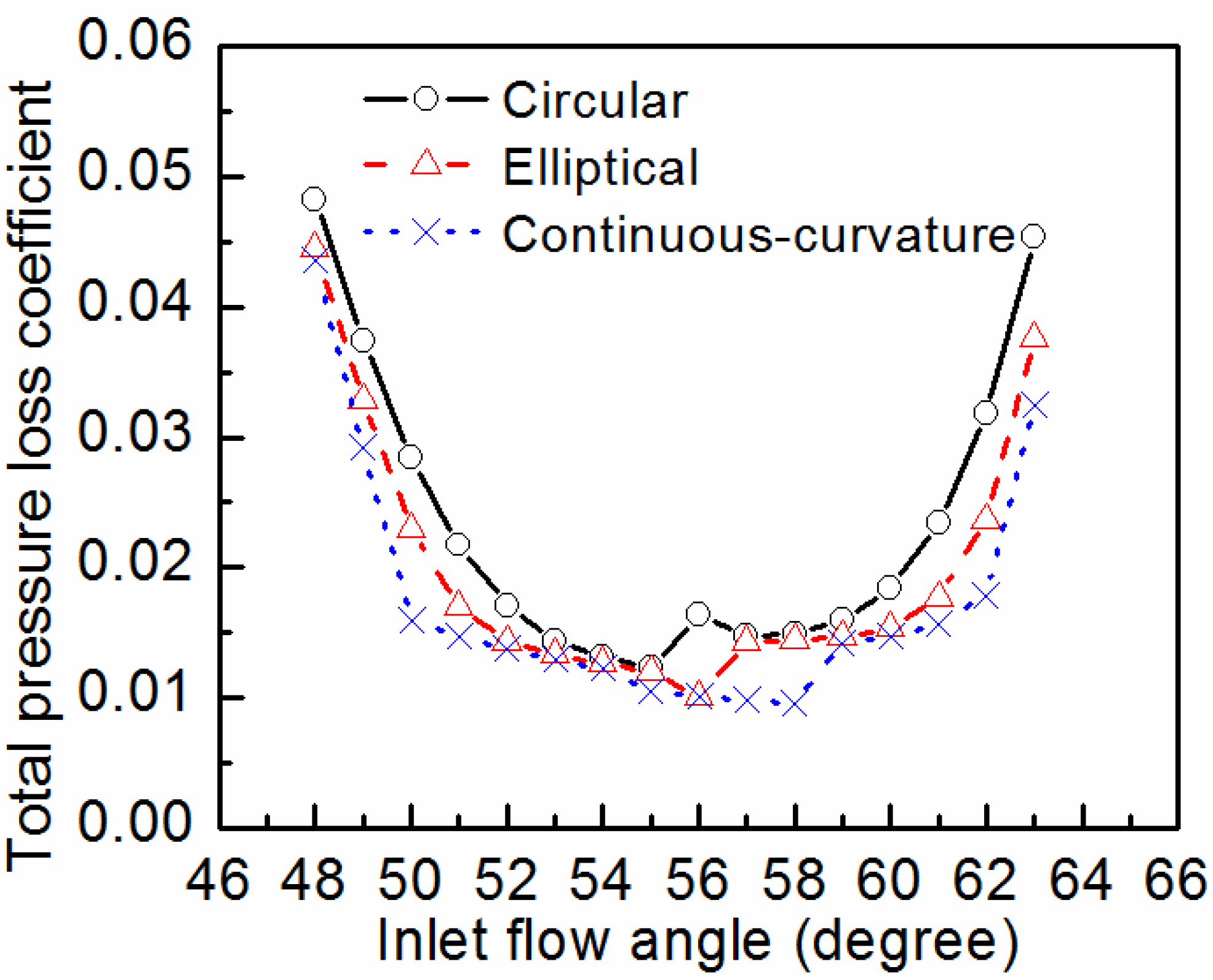
4.1. Effect of Curvature Continuity at the Leading Edge Blend Point

In order to study the effect of curvature continuity at the leading edge blend point, only the leading edge of the datum blade is optimized using the above-mentioned method. The optimized continuous-curvature leading edge as well as its curvature distribution is compared with conventional circular and elliptical leading edges in Figure 8 and Figure 9. It can be seen from Figure 9 that obvious curvature discontinuities exist at the blend points of blades with circular and elliptical leading edges, whereas the front-end curvature distribution of blade with the optimized leading edge is continuous (note that signs of the curvature values are neglect in the figures of this paper for simplicity).
Figure 8. Comparison between different leading-edge geometries: (a) circular LE; (b) elliptical LE (a/b = 2); (c) continuous-curvature LE.
Energies 07 08150 g008
Figure 9. Front-end curvature distributions of blades with different leading edges.
Energies 07 08150 g009
Figure 10 shows the calculated loss buckets of the blades with different leading-edge shapes. The blade with continuous-curvature leading edge achieves a 2.5° improvement in working range (the range of incidences with total pressure loss lower than twice minimum loss) compared with the circular-leading-edge blade, and a 1.2° improvement compared with the elliptical one. The minimum loss has also been reduced with the continuous-curvature leading edge. In order to investigate the reason of the performance improvement, the flow details at three different inlet flow angles are analyzed.
At the inlet flow angle α = 56°, the elliptical and continuous-curvature leading edges have similar losses, whereas the circular leading edge encounters an abrupt increase of loss (Figure 10). Figure 11 shows the suction-side pressure coefficient distributions around different leading edges at α = 56°, while Figure 12 compares the corresponding streamlines and turbulence intensity distributions. (Note that—Cp is shown in plots of pressure distribution, so the pressure spikes appear positive, and the streamwise location is normalized by the streamwise length of the blade surface.) For the circular leading edge, an obvious suction-side spike is observed. The flow accelerates quickly at the leading edge because of the small surface radius of curvature, and then starts to decelerate where the leading edge blends to the main surface, forming the pressure spike in Figure 11. The flow encounters large adverse pressure gradient because of the spike and separates close to the blend point, which can be seen from the streamlines in Figure 12a. The flow separation causes transition of the laminar boundary layer, as shown in the turbulence intensity distributions. The induced turbulent boundary layer then reattaches, forming the leading edge separation bubble in Figure 12a. The plateau of pressure in Figure 11 also shows the presence of the separation bubble. It has been claimed by Tain [2] and Goodhand [3] that this kind of separation bubbles results in a sharp increase in the trailing edge energy thickness, thus inducing a high loss. A smaller spike also exists in the pressure distribution of the elliptical leading edge, but the mild adverse pressure gradient does not cause the boundary layer to separate. As for the continuous-curvature leading edge, its pressure distribution is completely free of spike and no separation exists near the leading edge. The prevention of separation bubbles has resulted in the low losses of the elliptical and continuous-curvature leading edges.
Figure 10. Loss buckets of blades with different leading-edge shapes.
Energies 07 08150 g010
Figure 11. Pressure distributions at α = 56°.
Energies 07 08150 g011
Figure 12. Streamlines and turbulence intensity distributions at α = 56°: (a) circular LE; (b) elliptical LE; (c) continuous-curvature LE.
Energies 07 08150 g012
As shown in Figure 13 and Figure 14, at α = 58°, the flows around both circular and elliptical leading edges have suction-side spikes in their pressure distributions, and separation bubbles are induced, which cause large losses for the two. However, the elliptical leading edge exhibits a smaller separation bubble than the circular one, thus its loss is also a little smaller. At this flow angle, the continuous-curvature leading edge is still without a spike in its pressure distribution and can get the lowest loss.
Figure 13. Pressure distributions at α = 58°.
Energies 07 08150 g013
Figure 14. Streamlines and turbulence intensity distributions at α = 58°: (a) circular LE; (b) elliptical LE; (c) continuous-curvature LE.
Energies 07 08150 g014
As shown in Figure 15 and Figure 16, at α = 60°, all the three leading edges have induced separation bubbles and exhibit relatively high losses. However, the size of the separation bubble is obviously depressed for the continuous-curvature leading edge. Comparing the spikes induced by different leading edges reveals a special phenomenon that the continuous-curvature leading edge induces the highest spike at α = 60°. It can be seen from Figure 15 that the spike induced by the circular leading edge locates at a relative streamwise location of 0.4%, which corresponds to the blend point, and the spike location of the elliptical leading edge is basically the same as the circular one, only with a small advancement. However, the spike location of the continuous-curvature leading edge is much different, at a relative streamwise location of 0.08%, very near the leading-edge nose. The difference in spike locations indicates that the spike-generating mechanism of the continuous-curvature leading edge may be different, which will be discussed theoretically hereinafter.
Figure 15. Pressure distributions at α = 60°.
Energies 07 08150 g015
Figure 16. Streamlines and turbulence intensity distributions at α = 60°: (a) circular LE; (b) elliptical LE; (c) continuous-curvature LE.
Energies 07 08150 g016
The above analysis is based on the inlet turbulence intensity of 5%. Calculations at a high inlet turbulence intensity of 10% and a viscosity ratio of 100 have also been carried out for one typical inlet flow angle of 58°, and the results are presented in Figure 17. It can be found that the continuous-curvature leading edge is also beneficial in eliminating leading-edge separation at such high inlet turbulence intensity.
Figure 17. Streamlines and turbulence intensity distributions at high inlet turbulence intensity (α = 58°); (a) circular LE; (b) elliptical LE; (c) continuous-curvature LE.
Energies 07 08150 g017

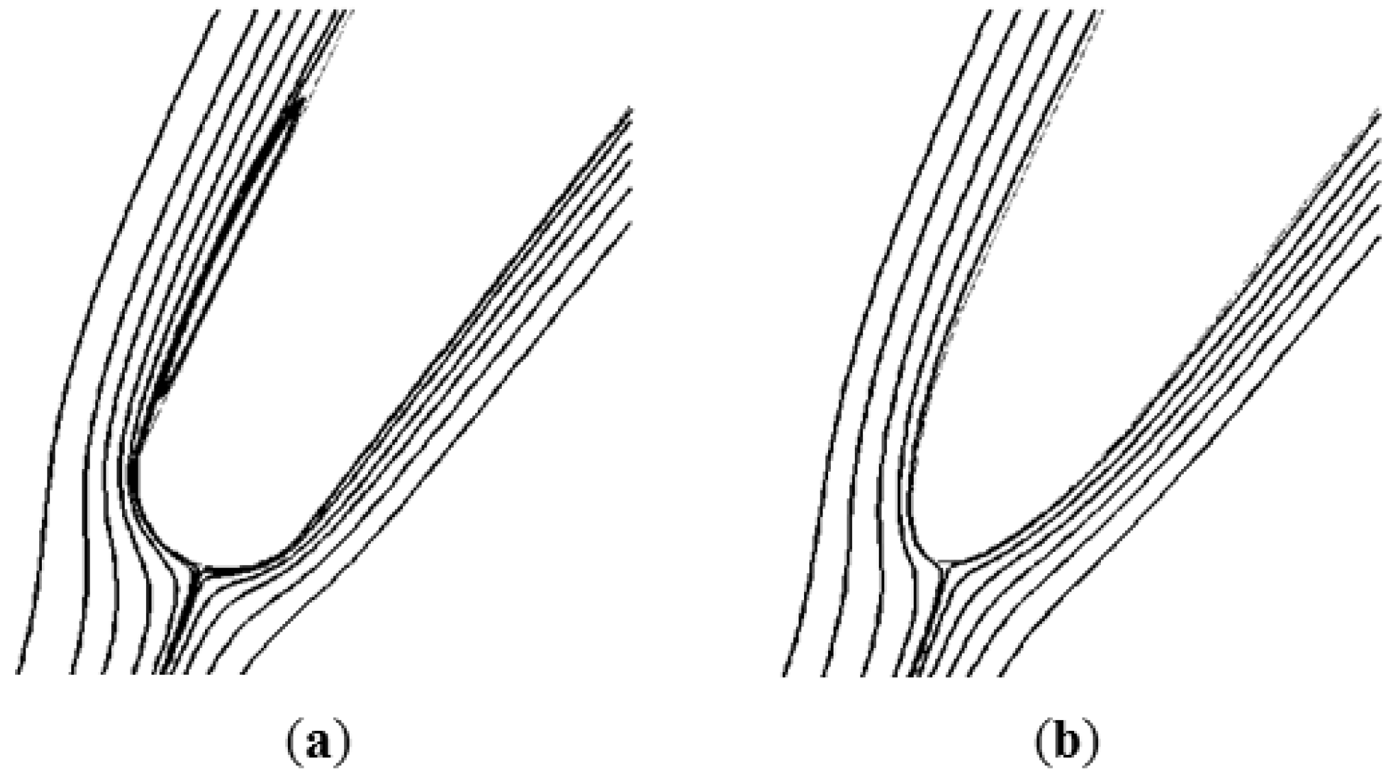
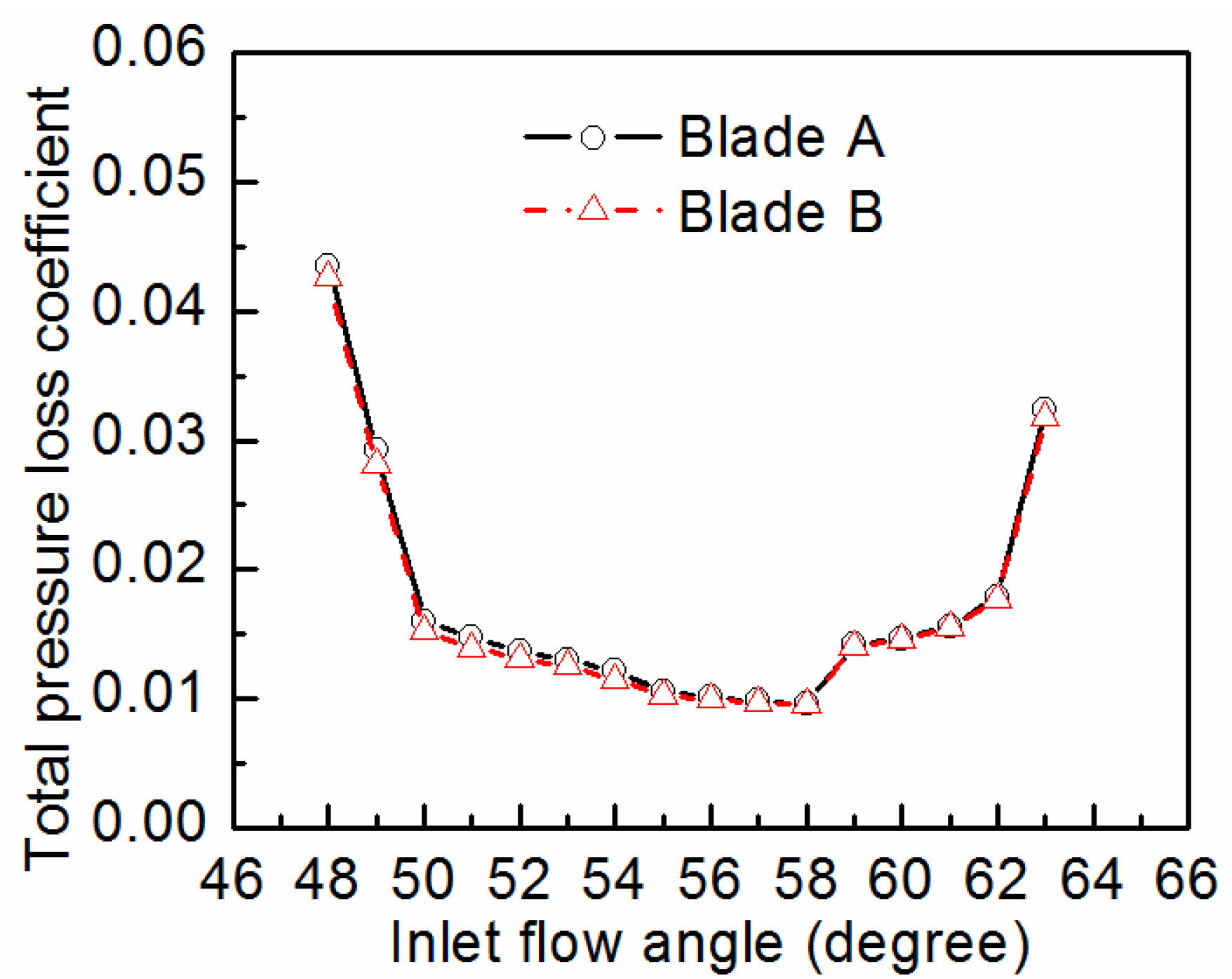
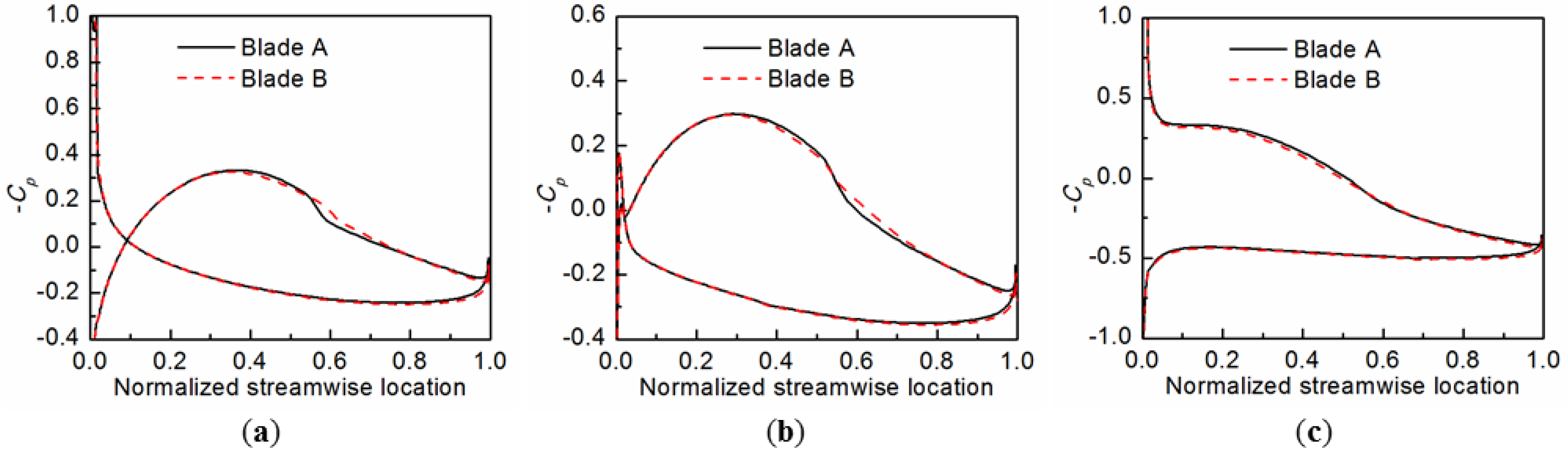
4.2. Effect of Curvature Continuity in the Main Surface

In order to study the effect of the main-surface curvature continuity, in this section the main blade surface is further optimized to be curvature-continuous and the resulted blade is denoted as Blade B, while the blade with only its leading edge optimized as described in the previous section is known as Blade A for comparison.
The main-suction-surface curvature distributions of Blade A and B are shown in Figure 18. Blade A, just like the datum blade, has discontinuous curvature or gradient of curvature in the main surface. (It should be noted that the datum curvature distribution is calculated by using 3-point difference method as in [14], so the discontinuities in curvature cannot be accurately captured.) But Blade B is represented by the B-spline curvature distribution, so the continuity of the curvature as well as the gradient of curvature is satisfied implicitly. Figure 19 compares the geometries of the two blades. The shape of Blade B is much similar to that of Blade A, with a maximum deviation around 0.1 mm, thus it is expected that any significant influence on blade performances would be caused by improvement of the curvature continuity rather than by the blade shape alteration.
Figure 18. Main-surface curvature distributions of Blade A and B.
Energies 07 08150 g018
Figure 19. Geometries of Blade A and Blade B (with parts of the suction surface enlarged).
Energies 07 08150 g019
The flowfields in two cascades using Blade A and B separately are also calculated by RANS computations with the same transition model. It can be seen from Figure 20 that the profile loss of Blade B is in general slightly lower than that of Blade A, but the improvement is much smaller than that by optimization of the leading-edge shape (Figure 10), indicating that the influence of main-part curvature continuity is not so remarkable as that of leading-edge curvature continuity.
Although the improvement by main-part continuous-curvature optimization is not so significant for the specific example, optimization methods prescribing the surface curvature distribution can still be regarded as effective tools for designing compressor blades for two reasons. Firstly, the pressure distributions at different inlet flow angles are smoother by the main-surface optimization, as shown in Figure 21, which will surely be beneficial for the blade performance. The small improvement in the performance of each blade row may result in visible accumulated improvement of multistage compressor performance. Secondly, the continuous-curvature optimization method is easy to realize, that is, there is no apparent increase in complexity of the blade representation method prescribing curvature distribution compared with the conventional ones, and meanwhile, it is suggested by Fathi and Shadaram [16] that the curvature-based optimization method can increase the speed of design process because of the closer relationship between design parameters with the flowfield.
Figure 20. Loss buckets of Blade A and B.
Energies 07 08150 g020
Figure 21. Pressure distributions of Blade A and B at different inlet flow angles: (a) α = 52°; (b) α = 55°; (c) α = 60°.
Energies 07 08150 g021

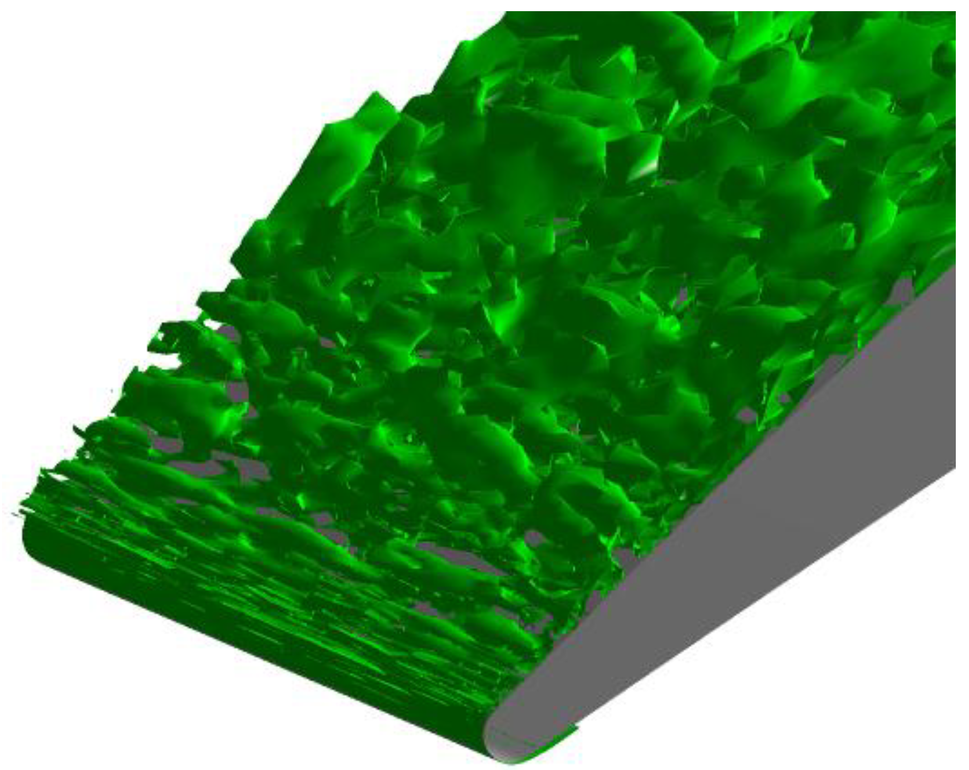
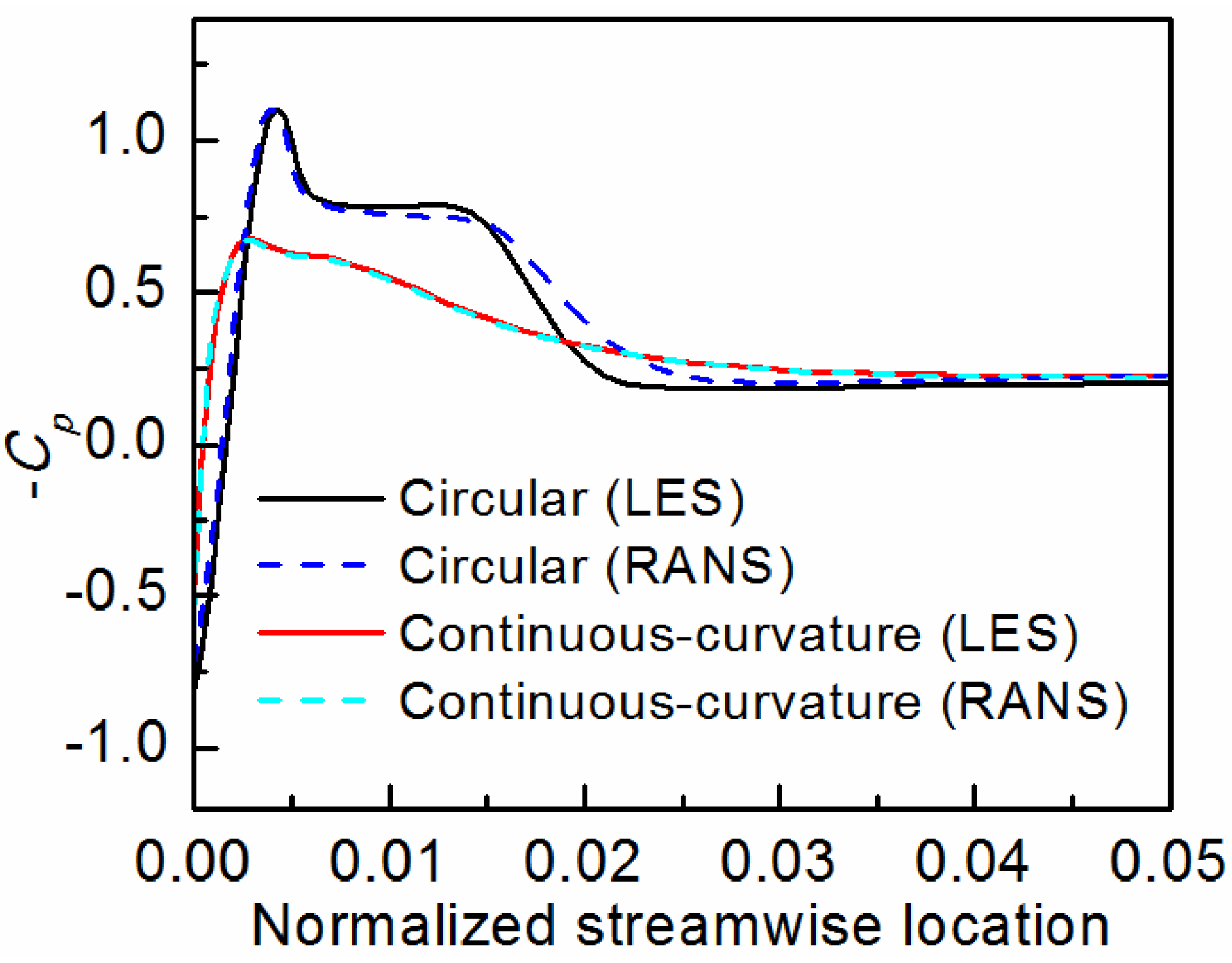
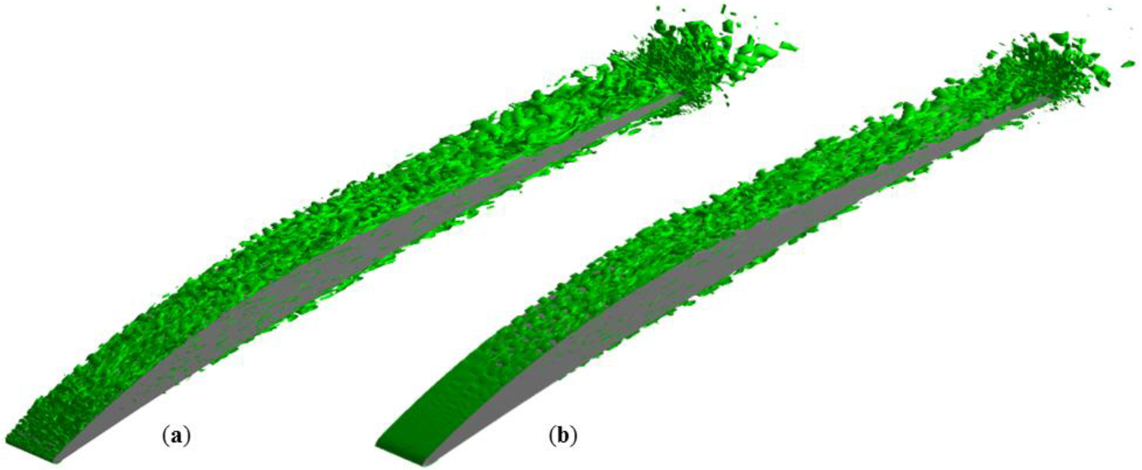
4.3. Validation of the RANS Computations with LES

Due to a lack of experimental data, LES is carried out to validate the above RANS computation results. Since the leading-edge curvature continuity seems to be more important than the main-part curvature continuity, the validation is focused on the effects of the leading-edge optimization. In the present research, the flowfields of blades with the conventional circular leading edge and the optimized continuous-curvature leading edge are calculated using LES at a singular inlet flow angle of 58° and a Reynolds number of 5 × 10⁵, which is limited by the author’s current computer resources.
The mesh used for 3D LES has a topology similar to that for 2D RANS computation in the blade-to-blade surface, but is three-dimensional and further refined to capture the large scale eddies. The total number of nodes is 3285500. The maximum normal distance of the nearest cell center to the blade surface is ∆n+ < 0.5, and the spanwise cell sizes are ∆z+ < 30. The commercial solver CFX is used to perform LES, with the wall-adapted local eddy-viscosity model [22] to take into account the sub-grid stress.
The instantaneous vortex structures on the suction side of the two cases are shown in Figure 22, with the Q-criterion [23] used to highlight the vortex cores. It can be seen that the transition of the laminar boundary layer has been delayed by the continuous-curvature leading-edge optimization. Initiation, instability, and transition of the spanwise K-H vortices produced by the leading-edge separation can be seen around the circular leading edge, as shown in Figure 23. It should also be noted that the number of grid points used in the present study is still limited by the current computer resources owned by the authors, and increased number of grid points will help to resolve more flow details as streamwise streaks in the transition process, as suggested in [24], and it will be one of the tasks for the authors’ future research.
Figure 22. Iso-surface of the Q-criterion on the suction side: (a) circular LE; (b) continuous-curvature LE.
Energies 07 08150 g022
Figure 23. Iso-surface of the Q-criterion around the circular leading edge.
Energies 07 08150 g023
The time-averaged pressure distributions for the two leading edges are compared in Figure 24. The calculated pressure distributions in RANS computations for the same Reynolds number are also presented to be compared with the LES results. For the blade with circular leading edge, both LES and RANS results show the spike and plateau of pressure, and the spike location and height as well as the initial position of separation predicted by RANS computations agree well with the LES results. For the blade with continuous-curvature leading edge, both methods show similar pressure distributions which are free of spike. Figure 25 shows the time-averaged streamlines by LES, which also confirm that the continuous-curvature leading edge has removed the pressure spike as well as the separation bubble.
Figure 24. Time-averaged pressure distributions at mid-span.
Energies 07 08150 g024
Figure 25. Time-averaged streamlines at mid-span (Re = 5 × 10⁵): (a) circular LE; (b) continuous-curvature LE.
Energies 07 08150 g025
LES is also performed at Re = 105, which corresponds to the low-Reynolds-number working conditions. As in Figure 26, a separation bubble appears around the blend point of the circular leading edge, similar to but longer than that at the higher-Reynolds-number condition.
Figure 26. Time-averaged streamlines at mid-span (Re = 105): (a) circular LE; (b) continuous-curvature LE.
Energies 07 08150 g026
The same variation of the bubble size with Reynolds number has been observed experimentally by Walraevens [1] and Perkins [25], which in turn can validate the present calculation results. It is also shown in Figure 26 that the flow around continuous-curvature leading edge is still free of separation even at such a low-Reynolds-number condition.

5. Theoretical Investigations

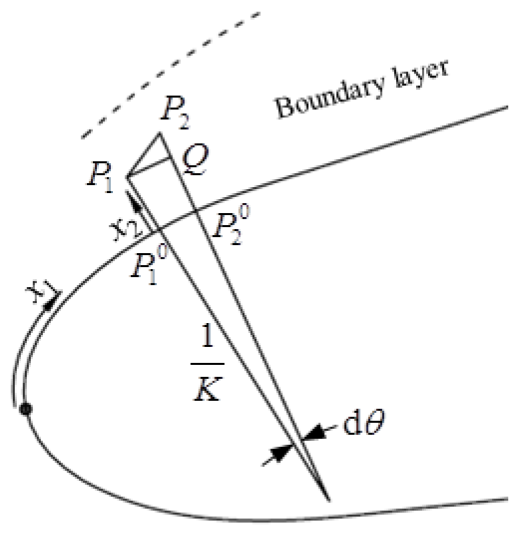
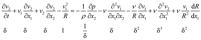
5.1. Analysis of the Boundary-Layer Equations for the Leading-Edge and Main-Surface Regions

In this section, the boundary-layer equations for flow along the blade surface are derived and used to seek a theoretical explanation of the continuous-curvature effects. Although the derivation of the boundary-layer equations for curved boundaries has been carried out by previous authors, e.g., Mager [26] and Rosenhead [27], the present study aims at offering a more precise and detailed derivation and comparison of the governing equations for the leading-edge region and the main-surface region, in which the respective roles and effects of curvature in the different regions can be shown.
As in [27], the general equations of the two-dimensional motion of a viscous fluid referred to an orthogonal curvilinear coordinate system are:
x 1 ( h 2 v 1 ) + x 2 ( h 1 v 2 ) = 0
v 1 t v 2 Ω 3 = 1 h 1 x 1 [ p ρ + v 1 2 + v 2 2 2 ] ν h 2 Ω 3 x 2
v 2 t + v 1 Ω 3 = 1 h 2 x 2 [ p ρ + v 1 2 + v 2 2 2 ] + ν h 1 Ω 3 x 1
where:
Ω 3 = 1 h 1 h 2 [ ( h 2 v 2 ) x 1 ( h 1 v 1 ) x 2 ]
As shown in Figure 27, the coordinate x1 is defined as the distance measured along the blade surface, and x2 the distance measured normal to the blade surface. Respect to the infinitesimal section P1P2 in Figure 27, the Lamé coefficients can be written as:
h 1 = P 1 Q d x 1 = [ R ( x 1 ) + x 2 ] R ( x 1 ) = 1 + K ( x 1 ) x 2
h 2 = P 2 P 2 0 P 1 P 1 0 d x 2 = 1
Figure 27. Coordinates for boundary-layer flow along the blade surface.
Energies 07 08150 g027
In the boundary layer near the leading edge and at the main surface, there always exists:
R > > x 2
Then Equations (16)–(21) can be reduced to:
v 1 x 1 + v 2 x 2 = 0
v 1 t + v 1 v 1 x 1 + v 2 v 1 x 2 + v 1 v 2 R = 1 ρ p x 1 + ν [ 2 v 2 x 1 x 2 + 2 v 1 x 2 2 + 1 R v 1 x 2 + 1 R v 2 x 1 1 R 2 v 1 ]
v 2 t + v 1 v 2 x 1 + v 2 v 2 x 2 v 1 2 R = 1 ρ p x 2 + ν [ 2 v 1 x 1 x 2 1 R v 1 x 1 + 2 v 2 x 1 2 + v 1 R 2 d R d x 1 ]
The orders of magnitude of variables in the above equations can be defined as:
x 1 , v 1 , p , ρ ~ O ( 1 )
x 2 , v 2 ~ O ( δ ) < < O ( 1 )
ν ~ O ( δ 2 )
The order of the curvature varies significantly where the leading-edge blends to the main surface, so the boundary-layer equations for the two different sections are derived respectively as follows.
For the main surface, the radius of curvature has the same order of magnitude as the characteristic length, i.e., R~O(1). Then the orders of different terms in Equations (24) and (25) are given under the equations:
Energies 07 08150 i001
Energies 07 08150 i002
On neglecting those terms with smaller orders of magnitude, the boundary-layer equations for the main surface can be written as:
v 1 t + v 1 v 1 x 1 + v 2 v 1 x 2 = 1 ρ p x 1 + ν 2 v 1 x 2 2
p x 2 = 0
which indicate that the effect of curvature on the main-part boundary layer can be neglected because of the large radius of curvature there. It is consistent with the above numerical results.
As for the leading-edge region, the curvature is much larger than that in the main surface. The radius of curvature R~O(RLE) does not have the same order as the characteristic length, so some of the terms including R may not be small enough to be neglected. Under this condition, Equations (24) and (25) can be rewritten as:
   v 1 t + v 1 v 1 x 1 + v 2 v 1 x 2 + K v 1 v 2 = 1 ρ p x 1 + ν ( 2 v 1 x 2 2 + K v 1 x 2 K 2 v 1 )
1 ρ p x 2 = K v 1 2
These equations indicate that curvature has important influence on the boundary-layer behavior around the leading edge. It should be noted that Equation (34) has the same form as the inviscid Bernoulli equation expressed in natural coordinates, which shows that the viscous effect in the normal direction is negligible in the boundary layer around curved surface.
To summarize, the above derivations help to confirm the numerical results about the curvature continuity effects, that is, the curvature continuity in the leading-edge region has significant effect on the blade loss, but the effect of curvature continuity in the main surface is much smaller. In addition, it should be noted that the effects of turbulence and compressibility have been neglected in the above analysis, which thus could be further improved accordingly.

5.2. Further Investigation of the Spike-Generation Mechanism

Since the effect of curvature continuity on the leading edge has much more significant effects on the blade performances and such effects are related to the pressure spikes near the leading edge, in this section the spike-generation mechanism and its relationship with the curvature continuity are further investigated based on the above boundary-layer equations.
The boundary-layer equation along the normal direction, i.e., Equation (34), is used to analyze the effects of curvature continuity at different incidences. Prior to the analysis, the assumption used thoughout should be mentioned, that is, it is assumed that the local variation of free-stream pressure is much less compared with that of the normal pressure gradient in the boundary layer, thus the streamwise increase of normal pressure gradient near the boundary will cause the streamwise decrease of near-wall pressure and vice versa.
At first, the streamwise pressure variations along different leading-edge shapes at the effective incidence of zero are analyzed. Figure 28 presents schematically streamwise variations of curvature and normal pressure gradient, in which the streamwise coordinate starts from the stagnation point. As shown in Figure 28a, when the airflow leaves the stagnation point and goes downstream along the circular leading edge, the streamwise velocity v1 firstly begins to increase. Since the wall curvature remains constant, according to Equation (34), the normal pressure gradient goes up because of the increase of velocity, which further results in a drop of near-wall pressure. The flow on the surface will in turn be accelerated by the streamwise decrease of pressure. Thus the velocity as well as the negative pressure coefficient rises rapidly with an increasing growth rate. However, when the flow passes the blend point, things become very different. Looking into the two adjacent points A and B located just before and after the blend point, it is found that the normal pressure gradients at the two points varies dramatically because of the curvature discontinuity at the blend point, which can be written as:
p x 2 | A = K L E ρ v 1 2 > > 0
p x 2 | B = K M a i n ρ v 1 2 0
Thus an abrupt decrease of normal pressure gradient will take place around the blend point as shown in Figure 28a (note that in the real environment the streamwise distribution of pressure gradient will show a rapid and continuous decrease, rather than a discontinuous decrease.) Since the free-stream pressure varies little between points A and B which are very close to each other, the rapid decrease of normal pressure gradient causes a steep decrease of –Cp, thus forming the leading-edge spike as previously mentioned.
Figure 28. Schematic streamwise variation of curvature and normal pressure gradient at zero effective incidence: (a) Circular LE; (b) Continuous-curvature LE.
Energies 07 08150 g028
As to the continuous-curvature leading edge, the curvature reaches its maximum value at the nose and then gradually decreases to near zero, as shown in Figure 9 and Figure 28b. At the effective incidence around zero, the stagnation point locates at the nose, so when the airflow goes downstream from the stagnation point, the streamwise velocity v1 begins to increase, whereas the curvature K decreases, and K v 1 2 as well as the normal pressure gradient will increase at first with a decreasing rate and decrease after a certain distance. Furthermore, since there exists no curvature discontinuity, no abrupt decrease of normal pressure gradient would occur. This kind of pressure-gradient variation (Figure 28b) results in a spikeless streamwise pressure distribution as in Figure 11, which prevents the leading edge separation. It should also be noted that the above theoretical analysis about the pressure distributions of different leading-edge shapes at zero incidences agrees with the numerical results as in Figure 11.
Figure 29 shows the schematic streamwise variations of curvature and normal pressure gradient at positive incidences. The streamwise coordinate again starts from the stagnation point, which is away from the nose under this situation. For the circular leading edge, the suction-side pressure variations are similar as those at zero incidence, only with increased spike heights because of the larger distance between the stagnation point and the blend point, as in Figure 29a.
Figure 29. Schematic streamwise variation of curvature and normal pressure gradient at a positive effective incidence: (a) Circular LE; (b) Continuous-curvature LE.
Energies 07 08150 g029
However, the flow conditions for continuous-curvature leading edge at a relatively large positive effective incidence may be much different. Under this condition, the stagnation point locates at a considerable distance apart from the nose on the pressure side, from where the curvature increases in the streamwise direction until the nose is reached. As shown in Figure 29b, the normal pressure gradient may at first rise rapidly because of the concurrent increase of K and v1 and almost reaches its maximum at the nose point, where K turns to decreasing very quickly with the normal pressure gradient starting to decrease a short distance downstream rather abruptly. It is this mechanism that induces the spike located very near the nose point as shown in Figure 15, where its generation has been questioned. It should also be noted that this effect would be significant only at incidences large enough for the airflow to obtain a considerable acceleration before reaching the nose, and at small positive incidences, the leading-edge pressure distribution is still favorable, as in Figure 13.
To verify the spike-generating mechanisms at large incidences for the different leading edges, the suction-side pressure distribution at α = 60° calculated by CFD and the curvature distributions are plotted together in Figure 30. The horizontal coordinate is the streamwise location normalized by the radius of circular leading edge with its range including the stagnation positions. It is clear that the spike and separation of the circular leading edge locates near the blend point, indicating that it is generated by the curvature discontinuity, whereas the spike of the continuous-curvature leading edge locates next to the nose point, indicating that it is generated by the large curvature at the nose point, which agrees with the above theoretical analysis. Like the blend-point spike, the nose-point spike also disrupts the boundary layer and induces a high loss. The loss buckets in Figure 10 show that when the flow angle becomes larger than 62 degrees, the loss of the continuous-curvature leading edge grows with a rate larger than that of the circular or elliptical leading edge. In addition, the moderate spike of the elliptical leading edge seems influenced simultaneously by the blend-point-curvature discontinuity and the large curvature at the nose point.
Figure 30. Relationship between suction-surface spike and curvature (α = 60°).
Energies 07 08150 g030
The above analysis reveals that a leading-edge spike may be controlled by a blend-point curvature discontinuity or a large nose curvature or both. At zero or small incidences the curvature discontinuity is the dominating factor, and at large incidences the effect of the large nose curvature becomes more significant. This can also help to explain the sharp-leading-edge paradox mentioned in the introduction. In general, a sharper leading edge usually represents a larger nose-point curvature with a smaller blend-point curvature discontinuity, so whether it is beneficial or harmful to the working range should be determined by the compromise of the two factors. It may also be noted that in most cases, such as the one in this paper, sharp leading edges help to enlarge the working range because the effect of large nose-point curvature only emerges at too high incidences. However, the maximum nose curvature must be limited as in the present leading edge optimization method, not only because of the structural constraint but also because of its harmful effects on aerodynamic performance at large incidences.

6. Conclusions

In this paper, an optimization method of continuous-curvature blade profile is proposed and the effects of curvature continuity on blade performances are investigated both numerically and theoretically. The RANS computations for blades with different leading-edge shapes show that the continuous-curvature leading edge reduces the minimum loss and enlarges the working range because the leading edge spike is removed with the separation bubble eliminated or reduced, and these results are confirmed with Large Eddy Simulations. It is also found that a large spike occurs very near the nose of the continuous-curvature leading edge when the incidence becomes large enough. Then, the effect of the continuous-curvature optimization for the main surface specifically is studied by comparing performances of the blade with only its leading edge optimized and the same blade with its main surface further optimized to be curvature-continuous but deviating little from the shape of the datum blade. RANS computations show that the performance improvement by the continuous-curvature optimization of the main surface is much smaller than that by the leading edge optimization. Although the direct improvement in blade performance is small, the continuous-curvature blade optimization method could still be regarded as an efficient tool for blade design because of the improvement in pressure distribution and the possible benefits in increasing the speed of design process.
Theoretical analysis based on proper boundary-layer equations in terms of order of magnitude gives a physical insight of the larger effects of the leading-edge-blend-point curvature continuity and the smaller effects of the main-surface curvature continuity. Then further investigations based on the boundary-layer equation around the leading edge demonstrate the different spike-generation mechanisms at zero and positive incidences. It is concluded that there exist two factors controlling the leading-edge spike, i.e., the curvature discontinuity at the blend point and the nose curvature. The former is dominant at zero or small incidences, while the latter becomes more important at larger incidences. To the authors’ knowledge, such dual spike-generating mechanisms have not been reported before. The sharp-leading-edge paradox can be explained accordingly, since sharper leading edge usually represents larger nose curvature and smaller blend-point curvature discontinuity as the elliptical one compared to the circular one. It should also be noted that in most cases, such as the one in this paper, the curvature discontinuity at the leading-edge blend point plays a more significant role within almost the whole effective incidence range, since the effect of large nose-point curvature only emerges at too high incidences, thus the leading edge shape with smaller blend point curvature discontinuity usually helps enlarge the working range of the compressor blade.

Acknowledgments

This work is supported by National Natural Science Foundation of China (Grant No. 51136003) and China Postdoctoral Science Foundation (Grant No. 2014M560965). An earlier version of this paper was presented at the conference Turbo Expo 2014.

Author Contributions

In this paper, Yin Song proposed the blade optimization method, did the analysis and wrote the manuscript; Chun-Wei Gu provided guidance for the numerical and theoretical analysis and polished the manuscript; Yao-Bing Xiao carried out part of the numerical calculation.

Nomenclature

C
chord length
Cp
pressure coefficient, C p = ( p p 1 ) / ( p t 1 p 1 )
Cx
axial chord length
di
distance between the point and the datum surface
h i or h 1 , h 2 , h 3
Lamé coefficients
K
curvature
K 0
nose curvature
k
slope of curve or turbulent kinetic energy
N i , j ( u )
basis functions of B-splines
n
number of B-spline control points
p
pressure or degree of B-splines
p 1
pressure at the inlet of the cascade
p t
total pressure
p t 1
total pressure at the inlet of the cascade
Q i
control points of B-splines
R
radius of curvature, R = 1 / K
Re θ
momentum thickness Reynolds number
S
streamwise length of the blade main surface
s
streamwise coordinate
T U
turbulence intensity, T U = ( 2 k / 3 ) 1 / 2 / U
U
knot vector of B-splines
u
parameter of B-splines
u i
components of B-spline knot vector
v i or v 1 , v 2 , v 3
components of velocity referred to an orthogonal curvilinear coordinate
X , Y
Cartesian coordinates of Bezier control points
x , y
Cartesian coordinates
x 1 , x 2 , x 3
coordinates of an orthogonal curvilinear coordinate system

Greek Symbols

α
inlet flow angle
γ
intermittency
δ
boundary layer thickness
ε i
constraint values
φ
slope angle
ν
kinematic viscosity
ρ
density
Ω i
components of vorticity
ω
total pressure loss coefficient

Abbreviations

LE
leading edge
LES
Large Eddy Simulation
RANS
Reynolds-averaged Navier-Stokes

Conflicts of Interest

The authors declare no conflict of interest.

References

  1. Walraevens, R.E.; Cumpsty, N.A. Leading edge separation bubbles on turbomachine blades. ASME J. Turbomach. 1995, 117, 115–125. [Google Scholar] [CrossRef]
  2. Tain, L.; Cumpsty, N.A. Compressor blade leading edges in subsonic compressible flow. J. Mech. Eng. Sci. 2000, 214, (Part C). 221–242. [Google Scholar] [CrossRef]
  3. Goodhand, M.N.; Miller, R.J. Compressor leading edge spikes: A new performance criterion. ASME J. Turbomach. 2011, 133, 021006:1–021006:8. [Google Scholar] [CrossRef]
  4. Giebmanns, A.; Backhaus, J.; Frey, C.; Schnell, R. Compressor leading edge sensitivities and analysis with an adjoint flow solver. In Proceedings of the ASME Turbo Expo 2013: Turbine Technical Conference and Exposition, San Antonio, TX, USA, 3–7 June 2013; ASME: New York, NY, USA, 2013. [Google Scholar]
  5. Tuck, E. A criterion for leading-edge separation. J. Fluid Mech. 1991, 222, 33–37. [Google Scholar] [CrossRef]
  6. Elmstrom, M.E.; Millsaps, K.T.; Hobson, G.V.; Patterson, J.S. Impact of nonuniform leading edge coatings on the aerodynamic performance of compressor airfoils. ASME J. Turbomach. 2011, 133, 041004:1–041004:9. [Google Scholar] [CrossRef]
  7. Carter, A. Blade profiles for axial-flow fans, pumps, compressors, etc. Proc. Instn. Mech. Engrs. 1961, 175, 775–806. [Google Scholar] [CrossRef]
  8. Liu, H.; Liu, B.; Li, L.; Jiang, H. Effect of leading-edge geometry on separation bubble on a compressor blade. In Proceedings of the ASME Turbo Expo 2003, collocated with the 2003 International Joint Power Generation Conference, Atlanta, GA, USA, 16–19 June 2003; ASME: New York, NY, USA, 2003. [Google Scholar]
  9. Lu, H.; Xu, L. Circular leading edge with a flat for compressor blades. J. Propuls. Technol. 2003, 24, 532–536. (In Chinese) [Google Scholar]
  10. Wheeler, A.P.S.; Sofia, A.; Miller, R.J. The effect of leading-edge geometry on wake interactions in compressors. ASME J. Turbomach. 2009, 131, 041013:1–041013:8. [Google Scholar] [CrossRef]
  11. Korakianitis, T.; Papagiannidis, P. Surface-curvature-distribution effects on turbine-cascade performance. ASME J. Turbomach. 1993, 115, 334–341. [Google Scholar] [CrossRef]
  12. Korakianitis, T. Prescribed-curvature-distribution airfoils for the preliminary geometric design of axial-turbomachinery cascades. ASME J. Turbomach. 1993, 115, 325–333. [Google Scholar] [CrossRef]
  13. Korakianitis, T.; Wegge, B.H. Three dimensional direct turbine blade design method. In Proceedings of the AIAA 32nd Fluid Dynamics Conference and Exhibit, St. Louis, MO, USA, 24–26 June 2002; AIAA: Reston, VA, USA, 2002. AIAA paper 2002-3347. [Google Scholar]
  14. Korakianitis, T.; Hamakhan, I.A.; Rezaienia, M.A.; Wheeler, A.P.S. Two- and three-dimensional prescribed surface curvature distribution blade design (circle) method for the design of high efficiency turbines, compressors, and isolated airfoils. In Proceedings of the ASME 2011 Turbo Expo: Turbine Technical Conference and Exposition, Vancouver, BC, Canada, 6–10 June 2011; ASME: New York, NY, USA, 2011. [Google Scholar]
  15. Sommer, L.; Bestle, D. Curvature driven two-dimensional multi-objective optimization of compressor blade sections. Aerosp. Sci. Technol. 2011, 15, 334–342. [Google Scholar] [CrossRef]
  16. Fathi, A.; Shadaram, A. Multi-level multi-objective multi-point optimization system for axial flow compressor 2D blade design. Arab. J. Sci. Eng. 2013, 38, 351–364. [Google Scholar] [CrossRef]
  17. Langtry, R.B. A Correlation-Based Transition Model Using Local Variables for Unstructured Parallelized CFD Codes. Ph.D. Thesis, University of Stuttgart, Stuttgart, Germany, 2006. [Google Scholar]
  18. Langtry, R.B.; Menter, F.R.; Likki, S.R.; Suzen, Y.B.; Huang, P.G.; Völker, S. A correlation-based transition model using local variables—Part II: Test cases and industrial applications. ASME J. Turbomach. 2006, 128, 423–434. [Google Scholar] [CrossRef]
  19. Langtry, R.B.; Menter, F.R. Correlation-based transition modeling for unstructured parallelized computational fluid dynamics codes. AIAA J. 2009, 47, 2894–2906. [Google Scholar] [CrossRef]
  20. Du, H.; Zhao, S.; Gong, J.; Lu, X.; Zhu, J. Effects of low-Reynolds number on flow stability of a transonic compressor. In Proceedings of the ASME Turbo Expo 2012, Copenhagen, Denmark, 11–15 June 2012; ASME: New York, NY, USA, 2012. [Google Scholar]
  21. Marciniak, V.; Longhitano, M.; Kügeler, E. Assessment of transition modeling for the design of controlled diffusion airfoil compressor cascades. In Proceedings of the ASME Turbo Expo 2013: Turbine Technical Conference and Exposition, San Antonio, TX, USA, 3–7 June 2013; ASME: New York, NY, USA, 2013. [Google Scholar]
  22. Nicoud, F.; Ducros, F. Subgrid-scale stress modelling based on the square of the velocity gradient tensor. Flow Turbul. Combust. 1999, 62, 183–200. [Google Scholar] [CrossRef]
  23. Jeong, J.; Hussain, F. On the Identification of a Vortex. J. Fluid Mech. 1995, 285, 69–94. [Google Scholar] [CrossRef]
  24. Gostelow, J.P.; McMullan, W.A.; Walker, G.J.; Mahallati, A. The role of streamwise vorticity in flows over turbomachine blade suction surfaces. In Proceedings of the ASME 2011 Turbo Expo: Turbine Technical Conference and Exposition, Vancouver, BC, Canada, 6–10 June 2011; ASME: New York, NY, USA, 2011; pp. 1091–1102. [Google Scholar]
  25. Perkins, S.; Henderson, A.D. Separation and relaminization at the circular arc leading edge of a controlled diffusion compressor stator. In Proceedings of ASME Turbo Expo 2012, Copenhagen, Denmark, 11–15 June 2012; ASME: New York, NY, USA, 2012; pp. 69384:1–69384:12. [Google Scholar]
  26. Mager, A.; Hansen, A. Laminar Boundary Layer over Flat Plate in a Flow Having Circular Streamlines; NACA Report No. TN-2658; NACA: Roxbury, MA, USA, 1952. [Google Scholar]
  27. Rosenhead, L. Laminar Boundary Layers: An Account of the Development, Structure, and Stability of Laminar Boundary Layers in Incompressible Fluids, Together with a Description of the Associated Experimental Techniques; Clarendon Press: Gloucestershire, UK, 1963; Chapter III. [Google Scholar]

