Reliability-Based Structural Optimization of Wave Energy Converters

Abstract

More and more wave energy converter (WEC) concepts are reaching prototype level. Once the prototype level is reached, the next step in order to further decrease the levelized cost of energy (LCOE) is optimizing the overall system with a focus on structural and maintenance (inspection) costs, as well as on the harvested power from the waves. The target of a fully-developed WEC technology is not maximizing its power output, but minimizing the resulting LCOE. This paper presents a methodology to optimize the structural design of WECs based on a reliability-based optimization problem and the intent to maximize the investor’s benefits by maximizing the difference between income (e.g., from selling electricity) and the expected expenses (e.g., structural building costs or failure costs). Furthermore, different development levels, like prototype or commercial devices, may have different main objectives and will be located at different locations, as well as receive various subsidies. These points should be accounted for when performing structural optimizations of WECs. An illustrative example on the gravity-based foundation of the Wavestar device is performed showing how structural design can be optimized taking target reliability levels and different structural failure modes due to extreme loads into account.

1. Introduction

Nowadays, the cost of electricity from wave energy converters (WECs) is estimated to be between 0.30 and 0.38 €/KWh [1]. This cost range is much higher compared with electricity from other renewable energy sources, like offshore wind or solar. Furthermore, no WEC technology has reached the commercial stage, where their electricity costs are as low as for offshore wind turbines, so far. Therefore, in order to drive the development of WECs further and make them competitive with other renewable electricity sources, the levelized cost of energy (LCOE) needs to be decreased. A possibility to decrease LCOE is by performing reliability-based structural optimizations. Other ways to decrease LCOE include arranging WECs in parks or using so-called hybrid solutions, where the WEC is embedded in other coastal or offshore structures, like offshore wind turbines, offshore platforms, ports or coastal defenses. An example of a hybrid WEC solution is given in [2].

Reliability-based optimizations do not focus on maximizing the harvested power output, but consider the whole system, including the benefit from selling electricity, expenses due to the structural design, structural failures, as well as maintenance and inspection costs. Reliability-based optimizations are used with success for (offshore) wind turbines in order to decrease LCOE; see, e.g., [3–5].

Maximization of harvested power may increase the income due to the sale of more electricity, but it also tends to increase loads on the structure, as shown in [6], where different control algorithms, as well as loads on welded details of the Wavestar are analyzed. Larger loads on the structure will increase the investment costs for a given working principle or, in general, lead to larger failure rates for a given design and, consequently, higher maintenance and inspection costs. Thus, it is important to focus on the whole system and the expected lifetime of the WEC in order to minimize the overall costs. This paper presents how you minimize overall costs for WEC applications with the aid of structural reliability assessments.

Structural reliability assessments are based on probabilistic approaches where uncertainties related to limited dataset lengths, measurements, considered models and physical parameters are included. Probabilistic reliability assessments can be used to define target reliability levels, as well as to calibrate partial safety factors (see, e.g., [7,8]).

Different development stages of a technology may lead to different optimal designs. At a prototype level, where subsidies for produced electricity are often available, the main purpose is checking the performance of the device, and when it comes to commercial stage, where no or limited subsidies are available and investors need to be convinced to invest in this kind of technology, the purpose will be minimizing LCOE in order to maximize the investor’s own benefit.

This paper shows a case study with a focus on the Wavestar device, where different development stages for a device are considered. The considered example focuses on reliability-based structural optimization of the gravity-based foundation of the Wavestar device, including the most common failure modes of the foundations. Furthermore, there is a discussion on some information about the probabilistic design of WEC structures, as well as the change of reliability-based optimal designs for different development stages of WECs.

2. Different Development Stages of a WEC Technology

When a new technology is under development, the structural design is driven by different objectives over time. Knowledge that is gained during ongoing development processes should be accounted for in the following development stage. Furthermore, financial subsidies, which may help to develop a new technology, do not always remain at the same level during the whole development process.

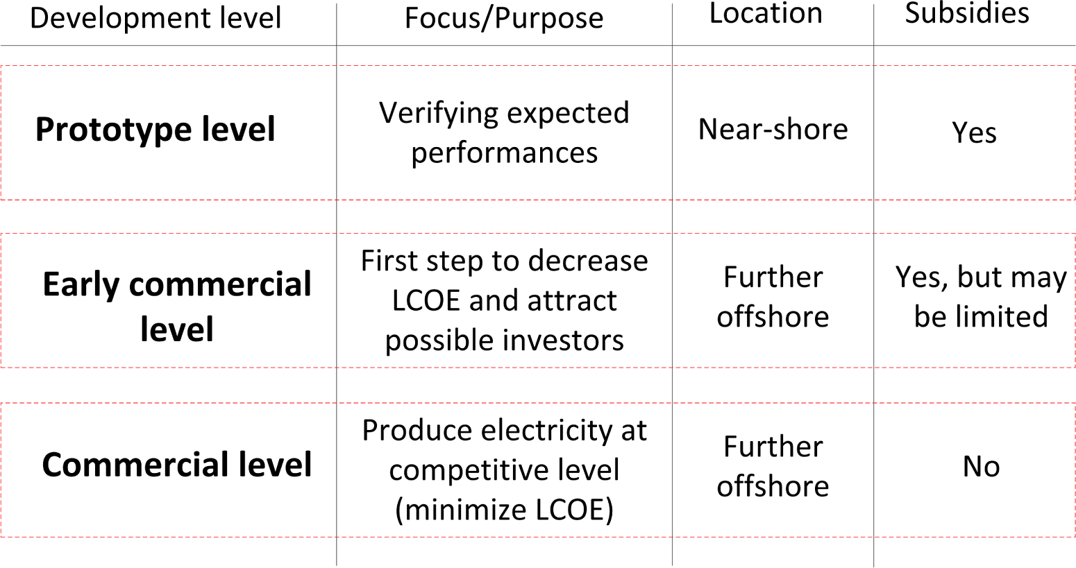
Figure 1 shows a flow chart of how a development process from the prototype level to the commercial level of a WEC concept could look like. In the first step, the prototype level shows that the expected power performance is as anticipated. Furthermore, knowledge that will be included for improvements in the next development stage needs to be gained. In order to hold the maintenance costs low and to guarantee the high accessibility of the device, the device should be placed near the shore. At this location, the wave power density can assumed to be low, which prevents extreme loads on the structure, which may lead to structural failure. When subsidies (e.g., per produced kWh electricity) are received, the low cost of electricity is not the focus for the prototype level. For a prototype, risk to a certain extent should be minimized due to the fact that, often, only one prototype is built, and the structural collapse of a prototype could mean the end for this company. Furthermore, failure of a prototype may not only have influence on the owner’s reputation, but also on the acceptance of a certain technology by society. Partial structural failure of the prototype leads to delays in the development process. However, it might be desired that a critical component fails at the prototype level, because the design can be easily adapted on this development level and only needs to be done for one prototype machine.

In the next development stage, which is here called the early commercial level, the technology is driven towards the commercial stage, and the knowledge gained during the prototype development stage is implemented, leading to design improvements. The focus during this development stage is to make the first steps towards decreasing LCOE in order to attract possible investors for this technology. These investments are necessary to bring the technology to a fully commercial stage. The device might be placed further offshore in order to increase the gained electricity. Subsidies may still be available, but might be smaller compared with subsidies at the prototype level.

Finally, when the technology reaches the commercial stage, the device is optimized in order to produce electricity at a competitive level. When a technology reaches a fully developed stage, subsidies cannot be expected anymore, and optimizations in order to decrease LCOE are based on the knowledge gained during the development process. In order to guarantee high power production, the commercial stage devices may be placed in high wave power density locations.

3. Probabilistic Structural Reliability Assessment

Optimization of WECs is performed in order to decrease the LCOE. The target of a fully-developed WEC technology is not to maximize its power output, but to minimize the resulting LCOE. For LCOE assessments, the overall system, including the structural design, should be considered. Structural design and its optimizations can be performed by using probabilistic reliability methods.

Probabilistic reliability assessments make it possible to include uncertainties related to the limited available data (statistical uncertainty), the simplified models used, e.g., to calculate loads/stresses (model uncertainties), uncertainties related to measurements (measurement uncertainties), as well as physical uncertainties due to Mother Nature (e.g., inter-annual variation of extreme values) for a certain failure mode. The statistical, model and measurement uncertainties are also called epistemic uncertainties and can be reduced when more information/knowledge becomes available. The physical uncertainties are also called aleatory uncertainties and cannot be reduced although more information becomes available.

The uncertainties in probabilistic reliability analyses are considered as stochastic variables, which are summarized in a vector called X = [X₁, X₂, …]. For a certain failure mode, a limit state equation, g(X, t), consisting of the resistance R(X, t) and the load S(X, t) can be established as a function of time t, if relevant as, e.g., for fatigue failures:

$$g(\mathrm{X},t)=R(\mathrm{X},t)-S(\mathrm{X},t)$$

(1)

From the limit state equation, based on Monte Carlo simulations or FORM/SORM techniques (first/second order reliability methods), the probability of failure, P_F, can be estimated for a certain failure mode and is equal to the probability that the limit state equation is smaller than or equal to zero. More information about probabilistic reliability methods for structural details can be found, e.g., in [9,10]. From FORM/SORM techniques, the so-called reliability index, β(X, t), is determined and can be used to estimate the probability of failure in the time interval [0, t]:

$$P_F(\mathrm{X},t)=P_F(g(\mathrm{X},t)\le 0)=\mathrm{\Phi }(-\beta (\mathrm{X},t))$$

(2)

where Φ() is the standardized normal distribution. The time interval, for which the reliability is estimated, is often assumed to be one year. The annual probability of failure, ΔP_F (X, t) given survival up to time t, can be estimated from the cumulative probability of failure (P_F (X, t)) at a certain time t:

$$\mathrm{\Delta }{P}_F(\mathrm{X},t)=\frac{P_F(t)-P_F(t-T)}{[1-P_F(t)]\cdot T}$$

(3)

where T = 1 year and t > T.

When performing reliability-based optimizations, target reliability levels need to be defined. The target reliability levels mainly depend on the consequences in the case of failure. In the case of structural failure, WECs have a low impact on the environment; there is no danger of fire and negligible danger of loss of human life, since they are operating unmanned. This means that the consequences in the case of failure are mainly of monetary value for WECs. [11] proposed minimal annual probabilities of failure for ultimate limit states in the range between 10⁻³ and 10⁻⁴, which is equal to a minimal annual reliability index, Δβ, of 3.1 and 3.7, for cases where the relative cost of the safety measure is large and the objective is to minimize the overall costs. The same annual maximal probability of the failure range is used for offshore wind turbines (see, e.g., [8]).

A structural component can often fail in different ways. Therefore, instead of focusing on just one failure mode, all possible modes for which a component might fail should be analyzed. Depending on whether each failure mode (serial system) or a combination of failure modes (parallel system) lead to the collapse of the structure, the total probability of failure can be estimated. When assuming that all considered failure modes lead directly to failure, the upper bound of the annual probability of failure, ΔP_F,sys, of the system is:

$$\mathrm{\Delta }{P}_{F,sys}={\displaystyle \sum _{i=1}^n\mathrm{\Delta }{P}_{F,i}}$$

(4)

where ΔP_F,i is the annual probability of failure for a certain failure mode i and n equals the number of considered failure modes.

4. Cost Models

In order to optimize the structural expenses, a cost model needs to be defined. The optimization proposed by [12] considers a purely monetary optimization, which can be applied for WECs due to the fact that the probability of the loss of human life is negligible. WECs are only manned during inspection and maintenance actions, which are performed during calm wave states (device accessible by boat) when storm events are unlikely to occur and the device is typically not in operation.

The purpose of an optimization is maximizing the profitability, W, which is the difference between the income (e.g., earned money from selling electricity) and the needed investment costs (e.g., building, maintenance and failure costs). It can be assumed that WECs are systematically reconstructed in the case of failure. In this case, the cost optimization problem can be written as [12]:

$$\begin{array}{c}\underset{\mathrm{z}}{\max }W(\mathrm{z})=\frac{b}{r{C}_0}-\frac{C_I(z)}{C_0}-\left(\frac{C_I(z)}{C_0}+\frac{C_F}{C_0}\right)\frac{\lambda P_F(z)}{r+\lambda P_F(z)}\\ s.t.z_i^l\le z_i\le z_i^u\\ \lambda P_F(\mathrm{z})\le \mathrm{\Delta }{P}_F^{\mathit{max}}\end{array}$$

(5)

where z = [z₁, …, z_n] indicates the main design variables, C_I(z) is equal to the initial building costs, C_F shows the expected direct failure costs, b is the yearly benefit from selling electricity, C₀ the reference costs and r shows the real rate of interest. Failure events are modeled by a Poisson process with annual rate λ. If the probability of failure is equal to P_F (z), the annual failure rate is equal to λP_F (z). The side constraints consider upper bounds z^u and lower bounds z^l for the design variables, as well as maximum annual failure rates $\mathrm{\Delta }{P}_F^{\mathit{max}}$ for a certain system that should not be exceeded.

An optimal design z^* can be determined as the solution from Equation (5). The annual probability of failure for a limit state equation g(X) of a certain failure mode can be estimated based on a probabilistic reliability assessment (see Section 3).

The cost model shown in Equation (5) is also applied to (offshore) wind turbine structure optimizations; see [3,4]. In Equation (5), it is assumed that only one device is considered. When more devices are considered and arranged in farms, the cost model should be written for the whole WEC farm and not only for a single device.

5. Case Study: Wavestar WEC

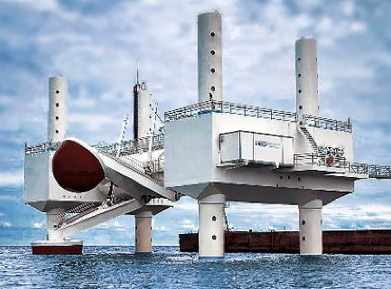
In this case study, the gravity-based foundation of the Wavestar WEC is considered. A prototype consisting of four piles, a platform and two floaters is installed near Hanstholm at the west coast of the Danish North Sea. Figure 2 shows a picture of the device. The floaters, which are moving when waves are passing, drive a hydraulic cycle, which impels a turbine and a generator for electricity production. The prototype produced electricity between January 2010, and September 2013. Its power capacity is equal to 110 kW (55 kW per floater). It needs to be mentioned that this WEC prototype is not optimized for the site where it is located. At the moment, remodeling work is going on in order to implement a new PTO (Power Take-Off) system (see [13]), as well as to install two additional floaters. The prototype is expected to come into service again in summer, 2015. The first commercial device will consist of 20 floaters with a total capacity of 600 kW (see [14]).

Three different development stages, as presented in Figure 1, are considered in this study.

Table 1. Considered development stages of the Wavestar concept.

Case	Development Level	Number of Floaters	Installed Capacity (kW)
1	Prototype	2	110
2	Pre-commercial	20	600
3	Commercial	(cost) data from offshore wind turbines

summarizes the installed capacity and number of installed floaters of the device. For the commercial device, no data is available, and therefore, (cost) data is taken from similar studies on offshore wind turbines.

This case study focuses on reliability-based optimization of the gravity-based foundation and the pile dimensions of the Wavestar device. The main design parameters for the foundation/pile are:

• Radius R of the foundation,

• Outer diameter D of the piles and

• Thickness t of the piles

which are used as design parameters and determined based on a reliability-based optimization. The considered failure modes, used to determine the values of the design parameter are:

$${}_{•\text{Overturning of device},}^{•\text{Sliding of the gravity-based foundation,}}\}\text{Focus on the complete Wavestar device}$$

$${}_{•\text{Bending capacity of piles}.}^{•\text{Soil bearing capacity failure and}}\}\text{Focus on one pile of the Wavestar device}$$

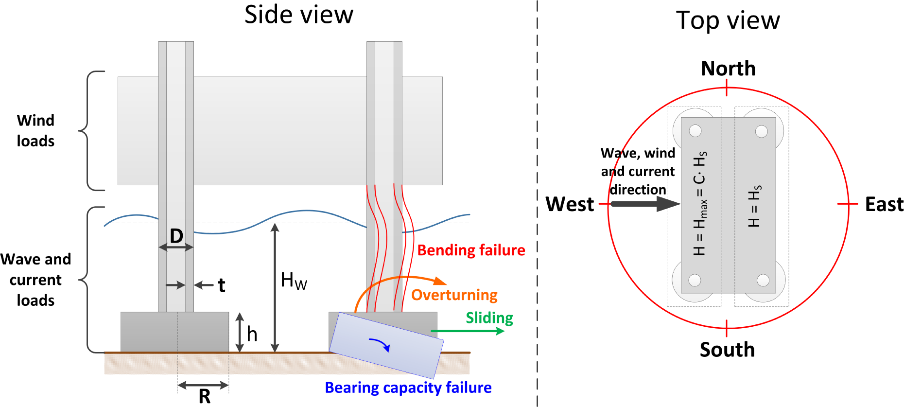
Figure 3 shows where the three optimization parameters are located at the device and to what the four considered failure modes can lead. The foundation is considered as concrete-based cylinder. More advanced foundation forms, like cone-shaped foundations, which may lead to further optimizations, are not investigated here. During storms, the floaters of the Wavestar are moved into storm protection mode. Therefore, for extreme wave and current loads, only the piles and the foundation need to be considered. Wind loads are considered on the platform. The diameter of the piles is assumed to be constant over height. A practical installation, which enables lifting and lowering of the whole platform, will disable the diameter change of the piles over height in the contemporary design. The load directions are assumed to be aligned and incoming from the west. Extreme loads due to extreme wave heights do not occur at all four piles at the same time. Therefore, for two piles, extreme significant wave height H_S is assumed to occur (see Figure 3, top view), whereas at the two other piles, the individual extreme wave height H_max, given extreme significant wave height H_S, is considered. The individual extreme significant wave height can be calculated as [15]:

$$H_{\mathit{max}}=C{X}_{meas}{X}_{st}{H}_S$$

(6)

where C is the factor leading from the significant wave height to the extreme individual wave height, X_meas represents the measurement uncertainty and X_st is equal to the climate statistics (including statistical uncertainty and inter-annual variation).

It is assumed, due to a lack of dynamic and frequency-related analyses for this static approach, that the moment of inertia of the piles (I_pile) remains constant for all different designs:

$$I_{pile}=\frac{\pi }{64}[D^4-{(D-2t)}^4]=0.172m^4$$

(7)

An important factor used for the considered limit state equations is the so-called eccentricity e, which occurs due to eccentrically-loaded foundations with a certain load W and a moment M due to wave, wind and current loads:

$$e=\frac{M}{W}=\frac{0.25M_{wi}+M_{Morison}}{0.25gW-F_b}$$

(8)

where M_wi is the moment at the foundation due to the wind acting on the platform of the device, M_Morison the moment due to Morison (current and wave) loads at the foundation and the pile, W the total weight of the device, g the gravitational acceleration and F_b the buoyancy force of the piles and the foundation in the water. The weight, W, of the whole WEC consists of the weight of the platform (W_platform), the piles (W_pile) and the foundation (W_foundation):

$$W=W_{platform}+4\underset{W_{pile}}{\underbrace{Dt\pi {\rho }_{steel}lg}}+4\underset{W_{foundation}}{\underbrace{R^2\pi h{\rho }_{concrete}g}}$$

(9)

where l is the length of the pile, g the gravitational acceleration, ρ_steel the density of steel and ρ_concrete the density of concrete. The weight of the platform (including the weights of the floaters) depends in this example on the development stage. The weight of the platform, W_platform, is assumed to be normal distributed with values shown in

Table 2. Stochastic model used for the different limit states explained in Sections 5.1, 5.2, 5.3 and 5.4. Values in () are only valid for Case 1. G, Gumbel distributed; N, normal distributed, LN, log-normal distributed; D, deterministic; COV, coefficient of variation; unc., uncertainty.

Name	Description	Type	Stochastic Model		Source
			Expected Value	COV
HS	Annual extreme sign. wave height	G	5.68 m (3.80 m)	0.02 (0.1)	[21,22]
Xmeas	HS measurement unc.	LN	1	0.03	[23]
Wplatform	Weight platform	N	375 tons (100 tons)	0.1	[3,14]
f	Friction coefficient	LN	0.4	0.15	[3]
Xm,s, Xm,ot, Xm,lb, Xbc	Model uncertainties static approach	LN	1	0.1	[3,11]
CD	Drag coefficient	LN	1	0.2	[11]
CM	Inertia coefficient	LN	2	0.15	[11]
XM	Model unc. Morrison Equation and water depth limits and linear wave model	LN	1	0.3	[11]
ρair	Density air	D	1.225 kg/m3
ρwater	Density water	D	1,000 kg/m3
ρsteel	Density steel	D	7,800 kg/m3
ρconcrete	Density concrete	D	2,300 kg/m3
r	Rate of interest	D	5%
l	Length pile	D	29 m (20 m)		[14]
h	Height foundation	D	1.5 m
L	Width Wavestar	D	17 m		[14]
A	Cross-section area Wavestar	D	455 m2 (210 m2)		[14]
C	Extreme individual wave height factor	G	1.86	0.09	[15]
Xst	Climate uncertainties	LN	1	0.05	[11]
K	Current velocity multiplicator	N	0.02	0.2	[24]
E	Young’s modulus steel	LN	2.1e5 MPa	0.02	[4]
XE	Model unc. Young’s modulus	LN	1	0.02	[4]
FY	Yield stress steel	DLN	240 MPa	0.05	[4]
XFY	Model unc. yield stress	LN	1	0.05	[4]
Xcr	Unc. critical load capacity	LN	1	0.1	[4]
ϕ	Friction angle	D	200
Xϕ	Unc. friction angle	LN	1	0.1	[11,25]
γ	Effective unit soil weight	LN	18 kN/m3	0.1	[11]
c	Soil cohesion	LN	80 kN/m3	0.4	[11]
XNγ	Model unc. Nγ	LN	1	0.06	[18]
XNc	Model unc. Nc	LN	1	0.3	[26]

.

The buoyancy force, F_b, of a hollow pile, which is filled with water, and a cylindrical foundation can be calculated in the following way:

$$F_b={\rho }_{water}g\pi (Dt(H_W-h)+R^{2}h)$$

(10)

where H_W is the water depth, ρ_water the water density, h the height of the foundation (=1.5 m) and D, t and R the optimization parameters.

Important for the limit states are the horizontal loads due to wind, current and waves. The wind load (F_wi) only acts on the platform of the device and can be calculated as:

$$F_{wi}=0.5{\rho }_{air}{C}_{D}A{V}_{wi}^2$$

(11)

where A is the cross-sectional area of the platform, ρ_air the air density, C_D the drag coefficient of the platform and V_wi the wind speed, which can be modeled conditional on the annual extreme significant wave height, as the wave load is the dominating load.

The total wave and current load on the pile is calculated based on Morison’s Equation and linear deep water wave theory:

$$F_{Morison}=\frac{\pi }{4}{\rho }_{water}{C}_M{D}^2{\displaystyle {\int }_{-H_W}^{H/2}{\dot{U}}_X(z)dz{X}_m+0.5{\rho }_{water}{C}_{D}D}{\displaystyle {\int }_{-H_W}^{H/2}{[V_c+U_X(z)]}^{2}dz{X}_m}$$

(12)

where U_X(z) is the horizontal wave-induced particle velocity, H_W is the mean water depth, H the considered wave height and V_c the current speed, which is assumed to be constant over depth. The modeling uncertainty, X_m, represents the model uncertainty considering deep linear theory instead of non-linear depth-limited waves. For estimating velocities above the mean water depth, Wheeler stretching [16] is used.

The moments shown in Equation (8) are calculated in the following. The moment at the foundation induced by the wind force F_wi is equal to:

$$M_{wi}=F_{wi}(H_W+5m)$$

(13)

The platform is mounted five meters above the water surface. The moments at the seabed due to waves and current are calculated from Morison loads as:

$$\begin{array}{r}{M}_{Morison}=\frac{\pi }{4}{\rho }_{water}{C}_M{D}^2{\displaystyle {\int }_0^{H_W+H/2}{\dot{U}}_X}(z)zdz{X}_m+\\ 0.5{\rho }_{water}{C}_{D}D{\displaystyle {\int }_0^{H_W+H/2}{[V_c+U_X(z)]}^{2}zdz{X}_m}\end{array}$$

(14)

In the following, the limit-state equations for the failure modes shown in Figure 3 are presented. Fatigue loads, which are not considered in this case study, may also have an influence on foundation design.

5.1. Sliding of Gravity-Based Foundation

The limit state equation for sliding of the gravity-based foundation due to extreme horizontal wave, wind and current loads is built up from [3]:

$$g_s=f(gW-4F_B)\frac{A_{eff}}{R^2\pi }-(4F_{Morison}+F_{wi})X_{m,s}$$

(15)

where W is the weight of the Wavestar device, f the friction coefficient, F_B the buoyancy force, R the radius of the foundation, A_eff the effective elliptical foundation area, F_Morison the wave and current loads, F_wi wind loads and X_m,s the uncertainty about the static load model, which accounts for dynamic responses. The effective elliptical foundation area (A_eff) can be calculated as:

$$A_{eff}=2R^2\arccos \left(\frac{e}{R}\right)-e\sqrt{R^2-e^2}$$

(16)

where R is the radius of the foundation and e the eccentricity (see Equation (8)). Table 2 presents the considered values and distribution parameters related to the failure mode ‘sliding of the gravity-based foundation’.

5.2. Overturning of Device

Failure mode ‘overturning of the Wavestar device’ considers the moment necessary to overturn the device. The general limit state equation can be written as:

$$g_o=(gW-4F_B)(0.5L+R-e)-(4M_{Morison}+M_{wi})X_{m,ot}$$

(17)

where g is the gravitational acceleration, L is the length of the device, R the foundation radius, e the eccentricity and X_m,ot the load model uncertainty (includes uncertainties about dynamic effects of the structure when considering a static approach). The total weight (W) of the Wavestar device is shown in Equation (9), the buoyancy (F_B) is presented in Equation (10) and the moments due to wind, wave and currents (M_wi and M_Morison) are given in Equations (13) and (14). The values and distribution parameters of the considered parameters in Equation (17) are presented in Table 2.

5.3. Bearing Capacity Failure

The bearing capacity depends on the soil properties. A limit state equation for the maximum load per square meter when eccentricity (e) occurs due to horizontal wind, wave and current loads can be derived, e.g., from [17] and leads to:

$$g_{cb}=q_{\mathit{max}}-\frac{0.25gW-F_b}{R^2\pi }\left(1+\frac{6e}{R}\right)X_{m,bc}$$

(18)

where q_max is the maximum pressure the soil can withstand and X_m,bc is the model uncertainty, which accounts for 3D effects, as well as dynamic responses.

The maximum soil pressure (ultimate bearing capacity) can be calculated according to Terzaghi’s superposition method and leads for a circular foundation on the seabed surface (see, e.g., [17,18]) to:

$$q_{\mathit{max}}=c{N}_c{E}_c{I}_c{X}_{Nc}+0.3\gamma 2R{N}_{\gamma }{E}_{\gamma }{I}_{\gamma }{X}_{N\gamma }$$

(19)

where γ is the effective soil weight, c the soil cohesion, R the radius of the foundation, N_γ the bearing capacity factor, E_γ and E_c the eccentricity factors due to bending moments, I_γ and I_c the inclination factors due to horizontal and vertical loads and X_Nγ, as well as X_Nc represent the model uncertainties related to the bearing capacity calculation. The eccentricity factor and inclination factor can be calculated according to [19] as:

$$\begin{array}{l}{I}_{\gamma }={\left(1-\frac{\alpha }{\varphi X_{\varphi }}\right)}^2,E_{\gamma }=1+0.1{\left[\tan \left(45+\frac{\varphi °X_{\varphi }}{2}\right)\right]}^2\\ I_c={\left(1-\frac{\alpha °}{90}\right)}^2,E_c=1+0.2{\left[\tan \left(45+\frac{\varphi °X_{\varphi }}{2}\right)\right]}^2\end{array}$$

(20)

where ϕ is the soil friction angle and α the inclination angle due to horizontal (F_H) and vertical loads (F_V):

$$\alpha =\frac{F_H}{F_V}=\arctan \left(\frac{gW-4F_B}{4F_{Morison}+F_{wi}}\right)$$

(21)

The bearing capacity factors N_c and N_γ can be calculated as [20]:

$$\begin{array}{l}{N}_{\gamma }=\frac{1}{2}\left(\frac{k_{p\gamma }}{{\cos }^2(\varphi X_{\varphi })}-1\right)\tan (\varphi X_{\varphi })\\ N_c=\left(\frac{\exp {(0.75\pi -\varphi X_{\varphi }/2)}^2}{2cos{(45°+\varphi °X_{\varphi }/2)}^2}-1\right)\cot (\varphi X_{\varphi })\end{array}$$

(22)

where X_ϕ represents the model uncertainty of the bearing capacity factor calculation. The passive earth pressure k_pγ is calculated dependent on the soil friction angle ϕ [20]:

$$k_{p\gamma }=5.82\exp (0.074\varphi X_{\varphi }),\varphi =15°-35°$$

(23)

The model uncertainty X_ϕ is assumed to be log-normal distributed as suggested in [11]. Table 2 shows values, and distribution types for other considered parameters.

5.4. Bending Capacity

The bending capacity of the pile depends on the used material and its dimensions. The critical bending capacity of a steel pile with diameter D and thickness t can be written according to [4] as:

$$M_{cr}=\frac{1}{6}\left(1-0.84\frac{D}{t}\frac{F_y{X}_{Fy}}{E{X}_E}\right)[D^3-{(D-2t)}^3]F_y{X}_{Fy}{X}_{cr}$$

(24)

where F_y is the yield stress of structural steel, including material uncertainties, E is the Young’s modulus of structural steel, X_Fy represents the model uncertainty about yield stress, the uncertainty about E is given by X_E and the overall model uncertainty of M_cr calculation is given by X_cr. Table 2 in shows the values and distribution types of the parameters presented in Equation (24).

The limit state equation for critical bending considering one pile is equal to:

$$g_{lb}=M_{cr}-(M_{Morison}+0.25M_{wi})X_{m,lb}$$

(25)

where X_m,lb represents the model uncertainty related to the considered static approach and possible 3D effects, which are not directly considered here.

5.5. Considered Cost Model

It is assumed that the WEC device is rebuilt in the case of structural failure, and therefore, the cost model presented by [12] (see Equation (5)) can be applied. The investment costs C_I(z) can be further separated in investment costs of the different Wavestar components. The following model is applied for the Wavestar device:

$$\frac{C_I(\mathrm{z})}{C_0}=C_{Foundation}(\mathrm{z})+C_{Piles}(\mathrm{z})+C_{Platform}+C_{Floaters}+C_{others}$$

(26)

where the investment cost for the foundation (C_Foundation(z)) and for the piles (C_Piles(z)) are dependent on the design parameters z. The costs for the platform (C_Platform), the floaters (C_Floaters) and, e.g., electricity cable to shore or installation costs, which are summarized in additional costs (C_others), remain constant for different design parameters z. The reference device leading to the reference costs, C₀, is chosen to be the prototype located at Hanstholm with:

• Foundation radius R₀ = 3.5 m,

• Pile outer diameter D₀ = 2 m,

• Length of pile l₀ = 20 m,

• Pile thickness t₀ = 60 mm and

• Foundation height h₀ = 1.5 m.

The relative cost distributions are approximated from preliminary studies from Wavestar, and the resulting optimized values may differ for different devices due to the fact that the considered device is a prototype. Therefore, it is assumed here that when the power plant is up-scaled and further developed, the design specifications (e.g., four piles, one platform) remain the same.

Table 3. The considered cost factors (portion of total investment costs when the reference device is built) and the cost function for dimension-dependent costs. R, radius of the foundation; h, height of the foundation; D, diameter of the piles; t, thickness of the piles.

Component Costs	Cost Factor (z = z0)	Cost Function
CFoundation (z)	$\frac{1}{10}$	$\frac{1}{10}\cdot \left(\frac{R^{2}h}{R_0^2{h}_0}\right)$
CPiles (z)	$\frac{1}{10}$	$\frac{1}{10}\cdot \left(\frac{Dtl}{D_0{t}_0{l}_0}\right)$
CFloaters	$\frac{7}{30}$	$\frac{7}{30}$
CPlatform	$\frac{7}{30}$	$\frac{7}{30}$
Cothers	$\frac{1}{3}$	$\frac{1}{3}$
CI(z = z0)	1

shows how the costs for the different Wavestar components change when the structural design is changed. The initial investment costs of the foundation are assumed to be proportional to the volume of the foundations and covers 10% of the overall total expenses. The cost about the piles for a certain design with pile diameter D and pile thickness t is assumed to be proportional to the material weight and equal to 10% of the total investment costs. The normalized resulting investment costs for the floaters (C_Floaters) and the platform (C_Platform) are assumed to be equally distributed and constant for the different foundation and pile dimensions. Furthermore, the other costs (C_other) are assumed to be constant for different foundation designs.

Due to the fact that no knowledge about the cost and relations between design parameters and resulting costs is available, assumptions have to be made. Furthermore, the design optimization strongly depends on the water depth (design of foundation) and the working principle of the device (loads on the structure). In this study, three different cases indicating different stages of development of the Wavestar device at two different locations are analyzed. The first case, Case 1, considers the Wavestar prototype located at Hanstholm. Case 2 represents the early commercial level (see Figure 1) where the Wavestar device is placed further offshore, which increases the failure costs, as well as the income from selling electricity due to larger wave resources. The commercial level is represented in Case 3. Due to a lack of experience and cost expectations for the pre-development level, as well as the commercial development level, the costs need to be taken from other offshore studies, which focus on reliability-based structural optimizations.

The income, b, due to selling electricity depends on the location (different wave resources), the number of installed floaters, the subsidies received per kWh produced electricity, as well as overall system optimizations, like, e.g., the energy conversion efficiency increase. The failure costs, C_F, depend on the experience and the resulting improvements, as well as the distance to shore and the wave environment. The benefits and the failure costs are different for the considered cases.

Table 4. The expected normalized failure costs (C_F/C₀), other costs (C_others) and the expected annual benefit (b/C₀) for different development stages of the Wavestar concept.

Case	Development Level	Failure Costs CF/C0	Benefit b/C0	Annual Electricity Production kWh/year	Electricity Prize DKK/kWh
1	Prototype	1/50	1/55 + 1/20	45,400	3.5
2	Pre-commercial	1/36	1/12	1.4 106	0.45
3	commercial	1/36	1/8	2.1 106	0.45

shows the considered normalized costs for the different cases.

For Case 1, the failure costs (C_F) are low due to the fact that direct access from shore, which lowers transportation costs, is possible. The benefit costs are estimated based on a feed-in tariff of 3.5 DKK (Danish krone)/kWh [27] for a WEC prototype. The Wavestar prototype is assumed to produce 45,400 kWh [28] of electricity annually. The benefit due to selling electricity is small and only 1/55 of the investment costs. However, the purpose of a prototype is also to gain knowledge and to improve the system. Therefore, for the prototype, there is an additional benefit, which is set equal to 1/20 of the investment costs and represents the system improvements, as well as the gain of information/knowledge used in the early commercial device. The further developed Wavestar concept (Case 2) is assumed to be placed further offshore. This increases the power output, but also increases the failure costs due to longer transportation routes and lower accessibility due to stronger environmental conditions. Due to the lack of failure cost estimations, the relative failure costs are taken from offshore wind turbine studies (see [4]). The early commercial Wavestar device is assumed to have 20 floaters and may be able to produce 1.4 GWh of electricity per year [29]. For the fully-developed Wavestar device (Case 3), no data and estimations about failure and benefit costs are available. Therefore, numbers used for offshore wind turbines from [3,4] for C_F/C₀, b/C₀ are considered in Case 3. The electricity feed-in tariff for Cases 2 and 3 is equal to 0.45 DKK/kWh, which is commonly used for offshore wind turbine assessments (see, e.g., [30]) in Denmark.

5.6. Stochastic Model

The environmental conditions are estimated from a 30-year hindcast simulation for the North Sea region at Hanstholm where wind speed, as well as significant wave height and mean zero-crossing wave periods are estimated. No current speed (V_c) data are available. According to [31], the current speed can be estimated from the wind speed V_wi:

$$V_c=0.916K{V}_{wi}$$

(27)

where K is assumed to be normal distributed with a mean value equal to 0.02 and a standard deviation of 0.004. The different objectives of different development levels of the Wavestar lead to different locations where the device should be placed. In order to account for that, two different locations are considered. For Case 1 (prototype level), a location (see

Table 5. Location dependent values from [21] for the different Wavestar cases.

Name	Latitude (0N)	Longitude (0E)	Depth HW (m)	Location for Cases
Location 1	8.620	57.129	10	Case 1
Location 2	8.582	57.131	19	Case 2, Case 3

) close to shore with low water depth is considered, whereas for the two others, the device is placed further offshore. At both locations, the seabed mainly consists of clay.

Table 2 presents the considered stochastic model for the different limit-states explained in Sections 5.1, 5.2, 5.3 and 5.4. The stochastic model for the environmental parameters (H_S, T, V_wi) is based on 30-year hindcast simulations (see [21]). The mean zero-crossing wave period (T), as well as the wind speed (V_wi) are assumed to be conditional on the significant wave height and log-normal distributed. A log-normal distribution for parameter X conditional on H_S looks like:

$$F_{X|H_S}(x|h)=\mathrm{\Phi }\left(\frac{\ln (x)-{\mu }_{X|H_S}}{{\sigma }_{X|H_S}}\right)$$

(28)

where ${\mu }_{X|H_S}$ and ${\sigma }_{X|H_S}$ are the conditional distribution parameters. The parameter ${\sigma }_{X|H_S}$ of the wind speed and the mean wave period is assumed to be constant for all H_S values. The distribution parameter ${\mu }_{X|H_S}$ is modeled with a linear relationship with H_S as performed, e.g., in [32].

Table 6. Conditional distribution parameters for mean zero-crossing wave period T and 10-min mean wind speed V_wi. The distribution parameters are based on a 30-year hindcast simulation [21]. Values in () are only valid for Case 1. LN, log-normal distributed.

Name	Description	Type	Distribution Parameters
			${\mu }_{{\mathrm{X}|\mathrm{H}}_{\mathrm{S}}}$	${\sigma }_{{\mathrm{X}|\mathrm{H}}_{\mathrm{S}}}$
T|HS	Conditional period mean wave	LN	0.30HS + 1.32 (0.12HS + 1.52)	0.12 (0.06)
Vwi|HS	Conditional wind speed	LN	0.50HS + 1.60 (0.16HS + 2.22)	0.13 (0.08)

shows the conditional distribution parameters for wind speed V_wi and mean wave period T of the two considered locations.

5.7. Results

Reliability-based optimization is performed based on FORM techniques, and the MATLAB-based FERUM4.1 program [33] is used. The expected lifetime of all considered devices is equal to 20 years, and the real rate of interest is equal to 5%. Due to the fact that four different failure modes are analyzed, the probability of the failure of the system needs to be assessed. It is assumed that the occurrence of one failure mode leads to the collapse of the overall structure. Furthermore, bearing capacity and bending failure consider one foundation and pile, respectively. The Wavestar consists of four piles and foundations, which need to be accounted for when estimating the overall system failure probability.

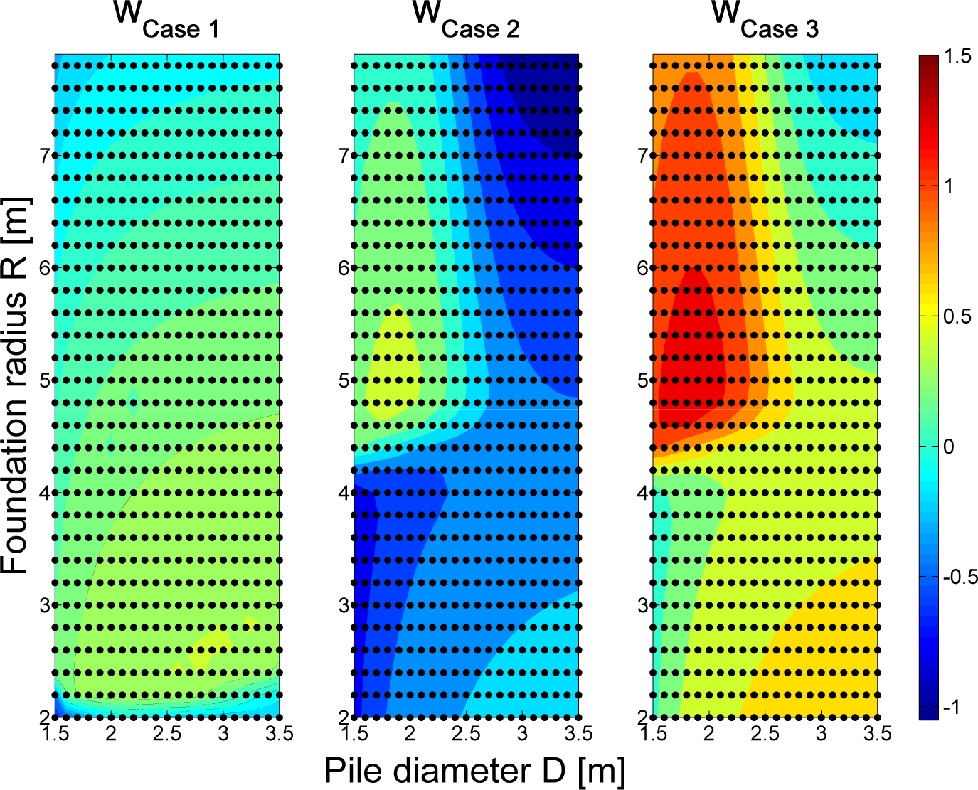
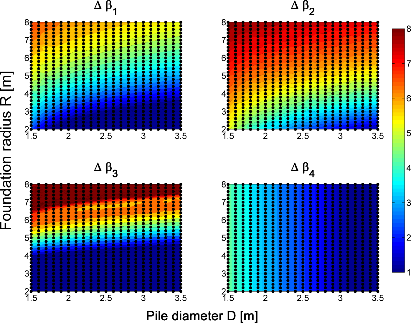
Figure 4 shows an example of how the reliability indices of the considered four failure modes behave dependent on the foundation diameter D and the foundation radius R for Case 3. Important for optimal design parameters is not only the reliability of the different failure modes, but the maximum profitability W (difference between the benefit and the total investment costs). Figure 5 shows different W values for the considered three cases.

Table 7. Foundation dimensions where the resulting profitability W is maximized for three cases with different development levels, including the reliability indices of the four different considered failure modes together with the total annual reliability index of the considered system (Δβ_sys). Δβ₁: annual reliability index sliding foundation; Δβ₂: annual reliability index overturning of device; Δβ₃: annual reliability index bearing capacity failure; Δβ₄: annual reliability index bending failure pile; W: benefit minus total costs over lifetime.

Case	Δβ1	Δβ2	Δβ3	Δβ4	Δβsys	D (m)	t (mm)	R (m)	W (−)
1	3.35	5.44	5.86	8.36	3.35	2.85	19.31	2.60	0.151
2	4.45	6.35	3.77	3.44	2.97	1.86	7.71	4.88	0.464
3	4.45	6.35	3.77	3.44	2.97	1.86	7.71	4.88	1.298

shows the resulting foundation and pile dimensions leading to maximized benefit minus total costs for the three different cases, including the resulting reliability indices for the four different failure modes. The reliability indices, as well as the dimensions D, t and R for Cases 2 and 3 are the same, because these two devices are assumed to be placed at the same location (same environmental conditions). For Case 1, the design is mainly driven by failure due to sliding of the gravity-based foundation. For Cases 2 and 3, the device is larger and placed at a location where the wave loads are increased. Therefore, the design for Cases 2 and 3 is mainly limited by the bearing failure of the seabed, as well as the bending failure of the piles. For all considered cases, overturning of the device is not of importance. The value of W is increasing when moving from the prototype (Case 1) over Case 2 (early commercial device) to Case 3 (commercial device) and, thus, increases the profitability of the investments. From the results in Table 7, it can be concluded that the optimal annual reliability index Δβ for components is around 3.3 and for the system reliability circa 3.0. More failure modes could decrease the system reliability, but due to the correlation of the considered failure modes, it is not assumed to result in a significant smaller reliability level.

As a side condition, the failure modes might be equal to or larger than a certain reliability index in order to fulfill a certain safety level.

Table 8. Foundation and pile dimensions where the profitability W is maximized for three cases with different development levels, including the reliability indices of the four different considered failure modes together with the total annual reliability index of the considered system (Δβ_sys), including a minimal annual reliability index for the different failure modes equal to or larger than 3.7 (Δβ_X ≥ 3.7) as a side condition. Δβ₁: annual reliability index sliding foundation; Δβ₂: annual reliability index overturning of device; Δβ₃: annual reliability index bearing capacity failure; Δβ₄: annual reliability index bending failure pile; W: benefit minus total costs over lifetime.

Case	Δβ1	Δβ2	Δβ3	Δβ4	Δβsys	D (m)	t (mm)	R (m)	W (−)
1	3.70	5.95	6.93	8.74	3.70	2.70	22.82	2.74	0.146
2	4.46	6.46	3.80	3.71	3.19	1.73	10.09	4.82	0.449
3	4.46	6.46	3.80	3.71	3.19	1.73	10.09	4.82	1.282

shows the resulting foundation and pile parameters when demanding annual failure indices of the considered failure modes to be larger or equal to 3.7. For Case 1, the probability of sliding of the device needs to be decreased, whereas for the two other cases, the reliability index related with bending failure of the piles needs to be increased. When introducing minimal annual reliability indices of 3.7, the profitability W decreases slightly (4% or less), which results from a change in the dimensions of the foundation and piles and leading to different loads on the structure, as well as to different investment costs. For all three cases, D decreases and R and t become larger when demanding a certain structural safety level (see Table 8) compared with no restrictions (see Table 7). This means that the safety level is mainly reached by decreasing the horizontal wave loads on the structure.

In general, the resulting optimal dimensions of the foundation and the piles, the reliability indices, as well as the value of W depend on the considered input costs. Therefore, a sensitivity analysis needs to be performed in order to assess the influence of certain input parameters. In the following, different values for the real rate of interest, the benefit and the expected failure costs are taken, and the impact on the profitability W, as well as the optimal foundation and pile dimensions are investigated.

5.7.1. Influence of Expected Failure Costs C_F

Changes in the failure costs, C_F, may change the maximum profitability W, as well as the corresponding dimensions of the piles and foundation.

Table 9. Profitability W for different development stages (cases) and different relative expected failure costs. C_F: expected cost in the case of failure; C₀: total investment cost.

Relative Failure Costs	Case 1	Case 2	Case 3
1.5 · CF/C0	0.149	0.464	1.297
1.0 · CF/C0	0.151	0.464	1.298
0.5 · CF/C0	0.150	0.465	1.298

shows the resulting profitability when varying the failure costs by ±50%. The differences in W are negligible when taking different failure costs. Furthermore, the cost-optimized dimensions are not affected by the failure cost range considered in Table 9. The optimal β-values (safety values) and dimensions of the piles and foundation remain the same for the expected failure cost range considered in Table 9.

5.7.2. Sensitivity of Income b

Changes in the benefit only affect the profitability W whereas the optimal design parameters, as well as the resulting reliability indices of the different failure modes remain the same.

Table 10. Profitability W for different development stages (cases) and different relative benefit values. b: benefit; C₀: total investment cost.

Relative Benefit	Case 1	Case 2	Case 3
1.1 · b/C0	0.257	0.631	1.548
1.0 · b/C0	0.151	0.464	1.298
0.9 · b/C0	0.045	0.298	1.048

shows the change in W for the three development stages dependent on the benefit changes. In general, W decreases when the relative income b/C₀ is decreased. The optimal β-values (safety values) and dimensions of the piles and foundation remain the same for the income range considered in Table 10.

An important aspect for the prototype level is that not only normalized financial benefit from selling electricity (= 1/55; see Table 4) is included, but also from gaining knowledge (= 1/20; see Table 4). When only the financial benefit from selling electricity is considered, the profitability W becomes equal to −0.627. Negative profitability means that the structure should not be built.

5.7.3. Sensitivity of Real Rate of Interest r

The influence of the considered real rate of interest, r, is assessed by using different r-values between 2% and 8%.

Table 11. Foundation and pile dimensions for Case 1 dependent on real rate of interest r. Δβ₁: annual reliability index sliding foundation; Δβ₂: annual reliability index overturning of device; Δβ₃: annual reliability index bearing capacity failure; Δβ₄: annual reliability index bending failure pile; Δβ_sys: total annual reliability index of the considered system; W: benefit minus total costs over lifetime.

r	Δβ1	Δβ2	Δβ3	Δβ4	Δβsys	D (m)	t (mm)	R (m)	W (−)
2%	3.57	5.97	6.84	8.28	3.57	2.84	19.52	2.76	1.735
5%	3.35	5.44	5.86	8.36	3.35	2.85	19.31	2.60	0.151
8%	3.21	5.56	5.39	8.23	3.21	2.86	19.10	2.54	−0.243

,

Table 12. Foundation and pile dimensions for Case 2 dependent on real rate of interest r. Δβ₁: annual reliability index sliding foundation; Δβ₂: annual reliability index overturning of device; Δβ₃: annual reliability index bearing capacity failure; Δβ₄: annual reliability index bending failure pile; Δβ_sys: total annual reliability index of the considered system; W: benefit minus total costs over lifetime.

r	Δβ1	Δβ2	Δβ3	Δβ4	Δβsys	D (m)	t (mm)	R (m)	W (−)
2%	4.58	6.47	4.03	3.63	3.20	1.77	9.25	4.92	2.931
5%	4.45	6.35	3.77	3.44	2.97	1.86	7.71	4.88	0.464
8%	4.36	6.10	3.67	3.34	2.85	1.91	7.02	4.87	−0.146

and

Table 13. Foundation and pile dimensions for Case 3 dependent on real rate of interest r. Δβ₁: annual reliability index sliding foundation; Δβ₂: annual reliability index overturning of device; Δβ₃: annual reliability index bearing capacity failure; Δβ₄: annual reliability index bending failure pile; Δβ_sys: total annual reliability index of the considered system; W: benefit minus total costs over lifetime.

r	Δβ1	Δβ2	Δβ3	Δβ4	Δβsys	D (m)	t (mm)	R (m)	W (−)
2%	4.58	6.47	4.03	3.63	3.20	1.77	9.25	4.92	5.014
5%	4.45	6.35	3.77	3.44	2.97	1.86	7.71	4.88	1.298
8%	4.36	6.10	3.67	3.34	2.85	1.91	7.02	4.87	0.375

show the annual reliability indices, the optimal dimensions and the profitability value W dependent on the real rate of interest for Cases 1, 2 and 3, respectively. A higher real rate of interests generally decreases the profitability, the reliability indices for the considered failure modes, as well as affects the optimal dimensions of the foundation and the pile. With a real rate of interest equal to 8%, the W values become negative for Cases 1 and 2. This means the overall benefit is lower than the costs, and therefore, it does not make sense to build these devices from an economical point of view.

In general, the optimization problem is very sensitive to the real rate of interest, and its value might even decide on the success or failure of the technology from an economical point of view.

6. Conclusions

This paper presents how structural designs of wave energy converters (WECs) can be optimized using a reliability-based approach. This optimization enables a decrease in the cost of energy in order for wave energy to become more competitive with other renewable electricity sources. The presented approach is used in nearby industries, like structures for wind turbines, and it assumes systematic rebuilding in the case of structural failure. Structural optimization may have different objectives for different steps of a technology development process. At a prototype level, the working principle needs to be tested and validated. Easy access to the device is important, and therefore, prototypes are often placed nearshore. Subsidies for produced electricity can be expected for prototypes. Hence, maximizing electricity production is not a major task for a prototype. When moving towards commercial devices, structural optimization becomes important, and the working principle is placed further offshore, where larger wave power resources appear and higher electricity production rates occur. Furthermore, knowledge gain should be accounted for when optimizing WEC systems.

This paper presents a case study, which focuses on reliability-based optimization of the structural design of the gravity-based foundation, showing how the methodology can be applied for WEC-specific designs. Parametric studies are performed in order to assess the influences and sensitivities of different input parameters on the overall design of the foundation. The case study shows that changes in income, e.g., due to selling electricity, will have a larger impact on the overall profitability of the device than changes in the expected failure costs. The real rate of interest is very important and may even decide over failure or success of a certain technology/design. The results indicate that the cost-optimal reliability level corresponds to an annual component reliability index of roughly 3.3 and an annual system reliability level around 3.0.

References

- The Carbon Trust, Accelerating Marine Energy—The Potential for Cost Reduction—Insights from the Carbon Trust Marine Energy Accelerator; The Carbon Trust: London, UK, 2011.
- Vicinanza, D.; Contestabile, P.; Quvang Harck Nørgaard, J.; Lykke Andersen, T. Innovative rubble mound breakwaters for overtopping wave energy conversion. Coast. Eng. 2014, 88, 154–170. [Google Scholar]
- Sørensen, J.D.; Tarp-Johansen, N.J. Reliability-based optimization and optimal reliability level of offshore wind turbines. Int. J. Offshore Polar Eng. 2005, 15, 141–146. [Google Scholar]
- Tarp-Johansen, N.J.; Sørensen, J.D.; Madsen, P.H. Experience with acceptance criteria for offshore wind turbines in extreme loading, In Proceedings of JCSS Workshop on Reliability Based Code Calibration, Zurich, Switzerland, 21–22 March 2002.
- Sørensen, J.D. Optimal, reliability-based turbine placement in offshore wind turbine parks. Civil Eng. Environ. Syst. 2007, 24, 99–109. [Google Scholar]
- Ferri, F.; Ambühl, S.; Fischer, B.; Kofoed, J.P. Balancing power output and structural fatigue of wave energy converters by means of control strategies. Energies 2014, 7, 2246–2273. [Google Scholar]
- Sørensen, J.D. Reliability-based calibration of fatigue safety factors for offshore wind turbines. Int. J. Offshore Polar Eng. 2012, 22, 234–241. [Google Scholar]
- Marquez-Dominquez, S.; Sørensen, J.D. Fatigue reliability and calibration of fatigue design factors for offshore wind turbines. Energies 2012, 5, 1816–1834. [Google Scholar]
- Madsen, H.O.; Krenk, S.; Lind, N.C. Methods of Structural Safety; Dover Publication Inc.: Mineola, NY, USA, 1986. [Google Scholar]
- Lemaire, M. Structural Reliability; ISTE Ltd.: London, UK, 2009. [Google Scholar]
- Probabilistic Model Code; Joint Committe on Structural Safety (JCSS): Zurich, Switzerland, 2001.
- Rackwitz, R. Risk control and optimization for structural facilities. Syst. Model. Optim. 2011, 130, 143–167. [Google Scholar]
- Hansen, R.H.; Kramer, M.M.; Vidal, E. Discrete displacement hydraulic power take-off system for the wavestar wave energy converter. Energies 2013, 6, 4001–4044. [Google Scholar]
- Kramer, M.M.; Marquis, L.; Frigaard, P. Performance evaluation of the wavestar prototype, In Proceedings of the 9th European Wave and Tidal Energy Conference (EWTEC), Southampton, UK, 5–9 September 2011.
- Ambühl, S.; Kofoed, J.P.; Sørensen, J.D. Influence of wave state uncertainties on probabilistic reliability assessments of wave energy devices, In Proceedings of the 10th European Wave and Tidal Energy Conference (EWTEC), Aalborg, Denmark, 2–5 September 2013.
- Wheeler, J.D. Methods for calculating forces produced by irregular waves, In Proceedings of the Offshore Technology Conference (OTC), Houston, TX, USA, 18–21 May 1969.
- Das, B.M. Principles of Foundation Engineering, Cengage Learning, 7th ed; Thomson Canada Ltd.: Toronto, ON, Canada, 2010. [Google Scholar]
- Ingra, T.S.; Baecher, G.B. Uncertainty in bearing capacity of sands. J. Geotech. Engrg. 1983, 109, 899–914. [Google Scholar]
- Meyerhof, G.G. Some recent research on the bearing capacity of foundations. Canad. Geotech. J. 1963, 1, 16–26. [Google Scholar]
- Terzhagi, K. Theoretical Soil Mechanics; John Wiley & Sons: New York, NY, USA, 1943. [Google Scholar]
- Tacher, E.; Thornfeldt Sørensen, J.V.; Golestani, M. Long-Term Wave Prediction—Deliverable D1.1. In Structural Design of Wave Energy Device (SDWED); Danish Hydraulic Institute (DHI): Hørsholm, Denmark, 2013. [Google Scholar]
- Ambühl, S.; Kofoed, J.P.; Sørensen, J.D. Stochastic modeling of long-term and extreme value estimation of wind and sea conditions for probabilistic reliability assessments of wave energy devices. Ocean Eng 2014, 89, 243–255. [Google Scholar]
- Allender, J.; Audunson, T.; Barstow, S.; Bjerken, S.; Krogstad, H.; Steinbakke, P.; Vartdal, L.; Borgman, L.; Graham, C. The WADIC project: A comprehensive field evaluation of directional wave instrcumentation. Ocean Eng 1989, 16, 505–536. [Google Scholar]
- Wind Turbines—Part 3: Design Requirements for Offshore Wind Turbines; IEC 61400-3; International Electrotechnical Commision: Geneva, Switzerland, 2009.
- Shahin, M.-A.; Cheung, E.M. Probabilistic analysis of bearing capacity of strip footings, In Proceedings of the 3rd International Symposium on Geotechnical Risk and Safety (ISGSR), Munich, Germany, 2–3 June 2011.
- Lee, I.K.; White, W.; Ingles, O.G. Geotechnical Engineering; Pitman Publishing Inc.: Boston, MA, USA, 1983. [Google Scholar]
- Nielsen, K.; Krogh, J.; Jensen, N.E.H.; Kofoed, J.P.; Friis-Madsen, E.; Mikkelsen, B.V.; Jensen, A. Bølgekraftteknologi: Strategi for Forskning, Udvikling og Demonstration; Aalborg University: Aalborg, Denmark, 2012; In Danish. [Google Scholar]
- Marquis, L.; Kristensen, B.; Vidal Sanchez, E. Vision and plans for wavestar development, In Proceedings of the 10th European Wave and Tidal Energy Conference (EWTEC), Aalborg, Denmark, 2–5 September 2013.
- Marquis, L.; Kramer, M.; Kringelum, J.; Fernandez Chozas, J.; Helstrup, N.E. Introduction of wavestar wave energy converters at the Danish offshore wind power plant horns rev 2, In Proceedings of the 4th International Conference on Ocean Energy (ICOE), Dublin, Irland, 17–19 October 2012.
- Munksgaard, J.; Morthorst, P.E. Wind power in the Danish liberalised power market-policy measures, price impact and investor incentives. Energy Policy 2008, 36, 3940–3947. [Google Scholar]
- Environmental Conditions and Environmental Loads; DNV RP C-205; Det Norske Veritas: BÃęrum, Norway, 2010.
- Christensen, C.F.; Arnbjerg-Nielsen, T. Return Period for Environmental Loads—Combination of Wind Wind and Wave Loads for Offhore Wind Turbines; Rambøll: Copenhagen, Denmark, 2000. [Google Scholar]
- FERUM: Finite Element Reliability Using Matlab, Available online: http://www.ce.berkeley.edu/projects/ferum/ accessed on 25 August 2014.