The Application of Discontinuous Galerkin Methods in Conjugate Heat Transfer Simulations of Gas Turbines

Abstract

The performance of modern heavy-duty gas turbines is greatly determined by the accurate numerical predictions of thermal loading on the hot-end components. The purpose of this paper is: (1) to present an approach applying a novel numerical technique—the discontinuous Galerkin (DG) method—to conjugate heat transfer (CHT) simulations, develop the engineering-oriented numerical platform, and validate the feasibility of the methodology and tool preliminarily; and (2) to utilize the constructed platform to investigate the aerothermodynamic features of a typical transonic turbine vane with convection cooling. Fluid dynamic and solid heat conductive equations are discretized into explicit DG formulations. A centroid-expanded Taylor basis is adopted for various types of elements. The Bassi-Rebay method is used in the computation of gradients. A coupled strategy based on a data exchange process via numerical flux on interface quadrature points is simply devised. Additionally, various turbulence Reynolds-Averaged-Navier-Stokes (RANS) models and the local-variable-based transition model γ-Re_θ are assimilated into the integral framework, combining sophisticated modelling with the innovative algorithm. Numerical tests exhibit good consistency between computational and analytical or experimental results, demonstrating that the presented approach and tool can handle well general CHT simulations. Application and analysis in the turbine vane, focusing on features around where there in cluster exist shock, separation and transition, illustrate the effects of Bradshaw’s shear stress limitation and separation-induced-transition modelling. The general overestimation of heat transfer intensity behind shock is conjectured to be associated with compressibility effects on transition modeling. This work presents an unconventional formulation in CHT problems and achieves its engineering applications in gas turbines.

1. Introduction

The continuous increase of the combustor outlet temperature has been producing incessant breakthroughs in the performance of modern aero engines and heavy-duty gas turbines. Accordingly, the thermal load of hot-end components has been steadily increasing, which necessitates the application of more complex cooling structures, such as various types of film cooling holes, impingement cooling holes, fins and serpentine-shaped channels, etc. The use of these structures increases the conjugate effects of heat transfer between hot flow, cooling flow and solid. It challenges engineers to precisely evaluate the lifetime of components or even the safety of whole engines, so the development of accurate and efficient conjugate heat transfer (CHT) simulation methods has become an important research area. In 1999, Martin et al. [1] developed a sequential conjugate strategy, by which a code for gas flow field computation and another one for solving heat conduction in solid blade was combined through an inner iteration process. This method taking advantage of available single-filed solvers had then been promptly adopted by some investigations [2,3,4,5,6], most of which used mature parabolic or elliptic equation solvers based on finite element (FE) methods in the solid domain. Meanwhile, partially aiming at enhancing the stability of the algorithm, the direct or full conjugate strategy [7,8,9,10,11] that integrates the governing equations in both fluid and solid domains using a single code also began to be developed and applied.

On or around the interface of two adjacent domains, the numerical accuracy together with the data exchange process has great effects on the computational performance in CHT problems. For improvement in this respect, more accurate algorithms can be enforced in both domains. Furthermore, more direct or localized process of data exchange is also rewarding. On these grounds, the discontinuous Galerkin (DG) methods can be considered to be applied in CHT simulations.

The DG methods that were first put forward by Reed and Hill [12] in 1973 and then further generalized by Cockburn and Shu [13,14,15,16], and Bassi and Rebay [17,18] have been successfully used in the simulations of inviscid, laminar and turbulent flows, to this day. The methods adopt the cell-wise approximate solutions in polynomial space based on the variational principle to obtain arbitrary high-order accuracy, whilst the eigen-decomposition (Riemann Solver usually) is used on cell-boundaries to account for the physics of wave propagation, which ensures good resolution of discontinuities. Comparing with the traditional finite volume (FV) framework for space discretization in computational fluid dynamics (CFD), the DG methods achieve high-order accuracy without the high-order interpolation process that comes at the expense of stencil expansions. As a consequence, it has better compactness and its solution accuracy has a lower dependence on the geometry and mesh properties. For the above reasons, together with the fact that it has been showing superior performance in CFD during last two decades, the introduction of DG methods to the whole domain of CHT problems can be beneficial for improving the accuracy in the region around the interface and localizing the data exchange process, and further enhancing the convergency and stability of the entire computation to some degree, especially in the situation of an interface with complex geometry or meshes of poor quality. Besides, one of the potential advantages of the idea is that the DG methods present a more natural way than the classic FE methods to represent the thermal discontinuities inside the solid, caused by thermal contact resistance [19], and so on.

In this paper, we present a primary framework for CHT simulations applying the DG methods on unstructured grids and a corresponding code fit for general engineering problems in gas turbines is developed. To this end, the compressible fluid dynamic equations and solid heat conduction equations are discretized in space and time under the unified algorithm. Taylor basis expandion at the centroid of each element, regardless of the element geometry type, is adopted. The Bassi-Rebay method [17], the ideology of which is borrowed from the mixed finite element method, is used to compute the gradients, including the temperature gradients of solids. A fully coupled strategy based on the data exchange process via the numerical flux of interface quadrature points is adopted. Moreover, considering the great effects of turbulence and transition behavior of boundary layer on the heat transfer, the code also assimilates various turbulence models and a local-variable-based two-equation transition model, γ-Re_θ developed by Menter and Langtry [20,21] in recent years. All the modeling equations are solved using the DG methods as the basis equations, consequently forming a coupling equation system under a unified algorithm. Some test cases are presented to validate the feasibility of the method. Then we apply it in the simulation and analysis of a convention cooled transonic turbine vane.

2. Discontinuous Galerki Methods for Conjugate Heat Transfer Problems

2.1. Fluid Domain

Here is a description of the DG methods we used in viscous fluid dynamics. The compressible Navier-Stokes or Reynolds-averaged Navier-Stokes (RANS) equations in the fluid domain Ω_F are given by:

$$\frac{\partial \mathbf{\text{U}}}{\partial t}+\frac{\partial {\mathbf{\text{F}}}_j}{\partial x_j}-\frac{\partial {\mathbf{\text{D}}}_j}{\partial x_j}=\mathbf{\text{S}},\text{ in }{\text{Ω}}_{\text{F}}$$

(1)

where:

$$\begin{array}{l}\mathbf{\text{U}}={\left[\begin{array}{ccccc}\text{ρ}& \text{ρ}{\mathbf{V}}^{\text{T}}& \text{ρ}E& {\mathbf{\text{U}}}^{\text{turbT}}& {\mathbf{\text{U}}}^{\text{tranT}}\end{array}\right]}^{\text{T}}\\ {\mathbf{\text{F}}}_j={\left[\text{ρ}{\text{u}}_j{\left(\text{ρ}\mathbf{V}{\text{u}}_j+\text{p}{\mathbf{e}}_j\right)}^{\text{T}}\text{ ρ}H{\text{u}}_j{\mathbf{\text{F}}}_j^{\text{turbT}}{\mathbf{\text{F}}}_j^{\text{tranT}}\right]}^{\text{T}}\\ {\mathbf{\text{D}}}_j={\left[0{\left(\underset{¯}{\mathbf{\text{T}}}\mathbf{\cdot }{\mathbf{e}}_j\right)}^{\text{T}}{\left(\left(\underset{¯}{\mathbf{\text{T}}}\mathbf{\cdot }\mathbf{V}-\mathbf{q}\right)\cdot {\mathbf{e}}_j\right)}^{\text{T}}{\mathbf{\text{D}}}_j^{\text{turbT}}{\mathbf{\text{D}}}_j^{\text{tranT}}\right]}^{\text{T}}\\ \mathbf{\text{S}}={\left[\begin{array}{ccccc}0& \mathbf{0}& 0& {\mathbf{\text{S}}}^{\text{turbT}}& {\mathbf{\text{S}}}^{\text{tranT}}\end{array}\right]}^{\text{T}}\end{array}$$

(2)

The total stress tensor $\underset{¯}{\mathbf{\text{T}}}$ is calculated by viscous constitutive relation (in which the molecular viscosity coefficient obeys the Sutherlands formula for air) and Boussinesq assumption, and the heat flux q is calculated by Fourier’s law (in which the thermal conductivity is λ = c_p(μ/Pr + μ_t/Pr_t). The turbulence and transition variables are calculated through the modeling equations which will be presented below. By means of the inner product of Equation (1) and a test function v in Ω_F and the Green’s formula, we obtain the semi-discrete weak formulation:

$$\begin{gathered} {\displaystyle \sum _{k=1}^n\left[{\displaystyle {\int }_{E_{\text{F}}^k}v\frac{\partial \mathbf{\text{U}}}{\partial t}\text{dΩ}}+{\displaystyle {\oint }_{\partial E_{\text{F}}^k}v\left({\widehat{\mathbf{\text{F}}}}_j-{\widehat{\mathbf{\text{D}}}}_j\right)n_j\text{dσ}}-{\displaystyle {\int }_{E_{\text{F}}^k}\frac{\partial v}{\partial x_j}\left({\mathbf{\text{F}}}_j-{\mathbf{\text{D}}}_j\right)\text{dΩ}}-{\displaystyle {\int }_{E_{\text{F}}^k}v{S}\text{dΩ}}\right]}=0, \\ \forall v\in L^2\left({\text{Ω}}_{\text{F}}\right) \end{gathered}$$

(3)

where ${\left\{E_{\text{F}}^k\right\}}_{k=1}^n$ is a complete element partition of Ω_F, ${\widehat{\mathbf{\text{F}}}}_j$ and ${\widehat{\mathbf{\text{D}}}}_j$ are inviscid and viscous numerical fluxes respectively. Assuming that the numerical solution ${\mathbf{\text{U}}}_{\text{h}}\in {\text{Γ}}_{\text{h}}^{\text{eq}}$ where:

$${\text{Γ}}_{\text{h}}=\left\{v\in L^2\left({\text{Ω}}_{\text{F}}\right):{v|}_{E_{\text{F}}^k}\in P^m\left(E_{\text{F}}^k\right)\text{, }\forall k\right\}$$

(4)

we can translate Equation (3) into the form:

$$\begin{gathered} {\displaystyle \sum _{r=0}^{l-1}\left(\frac{\text{d}{\tilde{\text{u}}}_r^k}{\text{d}t}{\displaystyle {\int }_{E_{\text{F}}^k}{\text{ϕ}}_r^k{\text{ϕ}}_s^k\text{dΩ}}\right)}=-{\displaystyle {\oint }_{\partial E_{\text{F}}^k}{\text{ϕ}}_{\text{s}}^k\left({\widehat{\mathbf{\text{F}}}}_j-{\widehat{\mathbf{\text{D}}}}_j\right)n_j\text{dσ}}+{\displaystyle {\int }_{E_{\text{F}}^k}\frac{\partial {\text{ϕ}}_s^k}{\partial x_j}\left({\mathbf{\text{F}}}_j-{\mathbf{\text{D}}}_j\right)\text{dΩ}}+{\displaystyle {\int }_{E_{\text{F}}^k}{\text{ϕ}}_s^k{S}\text{dΩ}}, \\ 0\le s\le l-1,\forall k \end{gathered}$$

(5)

${\left\{{\text{ϕ}}_s^k\right\}}_{s=0}^{l-1}$ is a set of complete basis of $P^m\left(E_{\text{F}}^k\right)$, and ${\widetilde{\mathbf{\text{u}}}}_s^k$ is one of the freedom of ${{\mathbf{\text{U}}}_{\text{h}}|}_{E_{\text{F}}^k}$ such that the expansion is satisfied:

$${{\mathbf{\text{U}}}_{\text{h}}\left(\mathbf{x},t\right)|}_{E_{\text{F}}^k}={\displaystyle \sum _{s=0}^{l-1}{\widetilde{\mathbf{\text{u}}}}_s^k\left(t\right){\text{ϕ}}_s^k\left(\mathbf{x}\right)}$$

(6)

For the calculation of gradients, the auxiliary variants P_j such that:

$${\mathbf{\text{P}}}_j-\frac{\partial \mathbf{\text{U}}}{\partial x_j}=0,\text{ in }{\text{Ω}}_{\text{F}}$$

(7)

are introduced. The weak form can be derived from the inner product of Equation (7) and a test function v in Ω_F:

$${\displaystyle \sum _{k=1}^n\left({\displaystyle {\int }_{E_{\text{F}}^k}v{\mathbf{\text{P}}}_j\text{dΩ}}-{\displaystyle {\oint }_{\partial E_{\text{F}}^k}v\widehat{\mathbf{\text{U}}}{n}_j\text{dσ}}+{\displaystyle {\int }_{E_{\text{F}}^k}\frac{\partial v}{\partial x_j}{U}\text{dΩ}}\right)}=0,\forall v\in L^2\left({\text{Ω}}_{\text{F}}\right)$$

(8)

Assuming the numerical solution ${\mathbf{\text{P}}}_{\text{h},j}\in {\text{Γ}}_{\text{h}}^{\text{eq}}$, we obtain the gradients calculation:

$${\displaystyle \sum _{r=0}^{l-1}\left({\widetilde{\mathbf{\text{p}}}}_{j,r}^k{\displaystyle {\int }_{E_{\text{F}}^k}{\text{ϕ}}_r^k{\text{ϕ}}_s^k\text{dΩ}}\right)}={\displaystyle {\oint }_{\partial E_{\text{F}}^k}{\text{ϕ}}_s^k\widehat{\mathbf{\text{U}}}{n}_j\text{dσ}}-{\displaystyle {\int }_{E_{\text{F}}^k}\frac{\partial {\text{ϕ}}_s^k}{\partial x_j}{\mathbf{\text{U}}}_{\text{h}}\text{dΩ}},0\le s\le l-1,\forall k$$

(9)

where ${\widetilde{\mathbf{\text{p}}}}_{j,s}^k$ is one of the freedom of ${{\mathbf{\text{P}}}_{\text{h},j}|}_{E_{\text{F}}^k}$ such that:

$${{\mathbf{\text{P}}}_{\text{h},j}\left(\mathbf{x},t\right)|}_{E_{\text{F}}^k}={\displaystyle \sum _{s=0}^{l-1}{\widetilde{\mathbf{\text{p}}}}_{j,s}^k\left(t\right){\text{ϕ}}_s^k\left(\mathbf{x}\right)}$$

(10)

In this paper, the All-Speed-Roe type scheme devised by Li and Gu [22] is selected as the inviscid numerical flux ${\widehat{\mathbf{\text{F}}}}_j$ in Equation (5) to guarantee its reasonable numerical dissipation in the situation of low Mach number, and consequently contributes improvements to the accuracy and stability in the boundary layer regions. The numerical flux ${\widehat{\mathbf{\text{D}}}}_j$ and $\widehat{\mathbf{\text{U}}}$ use the central scheme following [17].

2.2. Solid Domain

We use an analogous numerical method for the solid domain with the fluid one. The Fourier Equation in the solid domain Ω_S are given by:

$${\text{ρ}}_{\text{S}}{c}_{\text{p,S}}\frac{\partial T}{\partial t}+\frac{\partial q_j}{\partial x_j}=0,\text{ in }{\text{Ω}}_{\text{S}}$$

(11)

where:

$$q_j=-{\text{λ}}_{\text{S}}\frac{\partial T}{\partial x_j}$$

(12)

Analogizing with the DG manner Equations (3)–(6), we can derive the formulation:

$${\text{ρ}}_{\text{S}}{c}_{\text{p,S}}{\displaystyle \sum _{r=0}^{l-1}\left(\frac{\text{d}{\widetilde{\text{θ}}}_r^k}{\text{d}t}{\displaystyle {\int }_{E_s^k}{\text{ϕ}}_r^k{\text{ϕ}}_s^k\text{dΩ}}\right)}=-{\displaystyle {\oint }_{\partial E_s^k}{\text{ϕ}}_s^k{\widehat{q}}_j{n}_j\text{dσ}}+{\displaystyle {\int }_{E_s^k}\frac{\partial {\text{ϕ}}_s^k}{\partial x_j}{q}_{\text{h},j}\text{dΩ}},0\le s\le l-1,\forall k$$

(13)

where ${\widetilde{\text{θ}}}_s^k$ is one of the freedom of ${T_{\text{h}}|}_{E_s^k}$ such that:

$${T_{\text{h}}\left(\mathbf{x},t\right)|}_{E_s^k}={\displaystyle \sum _{s=0}^{l-1}{\widetilde{\text{θ}}}_s^k\left(t\right){\text{ϕ}}_s^k\left(\mathbf{x}\right)}$$

(14)

Equation (12) can be also transformed into the equation below as Equation (8) into Equation (10):

$${\displaystyle \sum _{r=0}^{l-1}\left({\widetilde{\text{η}}}_{j,r}^k{\displaystyle {\int }_{E_S^k}{\text{ϕ}}_r^k{\text{ϕ}}_s^k\text{dΩ}}\right)}=-{\displaystyle {\oint }_{\partial E_S^k}{\text{ϕ}}_s^k{\text{λ}}_S\widehat{T}{n}_j\mathrm{d\sigma }}+{\displaystyle {\int }_{E_S^k}\frac{\partial {\text{ϕ}}_s^k}{\partial x_j}{\text{λ}}_S{T}_h\text{dΩ}},0\le s\le l-1,\forall k$$

(15)

where ${\tilde{\eta }}_{j,s}^k$ is one of the freedom of ${q_{h,j}|}_{E_S^k}$ such that:

$${q_{h,j}\left(\mathbf{x},t\right)|}_{E_S^k}={\displaystyle \sum _{s=0}^{l-1}{\widetilde{\text{η}}}_{j,s}^k\left(t\right){\text{ϕ}}_s^k\left(\mathbf{x}\right)}$$

(16)

Again the central scheme is used for the numerical flux ${\widehat{\text{q}}}_j$ and $\widehat{T}$.

2.3. Fluid-Solid Interface

The continuity in physics of the temperature and normal heat flux on the fluid-solid interface should be ensured in any computational process. For this purpose, the precept is adopted that in each time step, the value of temperature computed from the side of solid domain is specified to the side of fluid meanwhile that of normal heat flux computed from the side of fluid domain is specified on the solid side, and the updated data will be treated as new boundary conditions of the respective domains in the next time step. In the DG framework, the solution distribution in each cell is naturally known at a certain time step. If the interface mesh on one side is consistent with that on the other (the situation in which the cases of this paper are), the above data exchange process can be directly achieved via the numerical flux calculations at quadrature points of the interface, without any interpolation. For any monotonicity preserving flux scheme represented by local variables on two sides of cell-boundaries, the numerical flux on the fluid side of the interface can be written as:

$$\widehat{\mathbf{\text{U}}}=\mathbf{\text{U}}\left({T|}_{\text{Solid}},\cdots \right)\text{, }{\widehat{\mathbf{\text{F}}}}_j={\mathbf{\text{F}}}_j\left({T|}_{\text{Solid}},\cdots \right)\text{, }{\widehat{\mathbf{\text{D}}}}_j={\mathbf{\text{D}}}_j\left({T|}_{\text{Solid}},{q_j|}_{\text{Fluid}},\cdots \right)$$

(17)

and the flux on the solid side can be:

$$\widehat{T}={T|}_{\text{Solid}}\text{, }{\widehat{q}}_j={q_j|}_{\text{Solid}}+\left({q_k|}_{\text{Fluid}}-{q_k|}_{\text{Solid}}\right)n_k{n}_j$$

(18)

The formulations of Equations (17) and (18) can implicitly guarantee the thermal coupling workable.

2.4. The Taylor Basis

In the framework, we choose the Taylor series expansion at the centroid of each element as the basis functions to represent the numerical polynomial solutions. The basis can be constructed naturally while generating a mass matrix with relatively small stiffness, and also enable the formulation adaptive to any types of element geometry. Considering the two-dimensional situation, for example, and aiming at rewriting Equation (6) (similarly for the Equations (10), (14) and (16)) as the series formula:

$${\mathbf{\text{U}}}_{\text{h}}\left(x,y,t\right)={{\mathbf{\text{U}}}_{\text{h}}|}_c{\text{φ}}_{00}+{\displaystyle \sum _{0\text{<}r+s\le l}\left({\frac{{\partial }^{r+s}{\mathbf{\text{U}}}_h}{\partial x^r\partial y^s}|}_c{\left(\Delta x\right)}^r{\left(\Delta y\right)}^s\right)}{\text{φ}}_{rs},r+s\le l,\left(x,y\right)\in E^k$$

(19)

where the subscript c represents the values at the centroid of E^k, we can derive a set of appropriate basis functions as:

$${\text{φ}}_{00}=1$$

(20)

and:

$$\begin{gathered} {\text{φ}}_{rs}=\frac{{\left(x\text{-}{x}_c\right)}^r{\left(y\text{-}{y}_c\right)}^s}{r\text{!}s\text{!}{\left(\Delta x\right)}^r{\left(\Delta y\right)}^s}-\overline{\frac{{\left(x\text{-}{x}_c\right)}^r{\left(y\text{-}{y}_c\right)}^s}{r\text{!}s\text{!}{\left(\Delta x\right)}^r{\left(\Delta y\right)}^s}}\text{=}\frac{{\left(x\text{-}{x}_c\right)}^r{\left(y\text{-}{y}_c\right)}^s}{r\text{!}s\text{!}{\left(\Delta x\right)}^r{\left(\Delta y\right)}^s}-\frac{1}{\left|E^k\right|}{\int }_{E^k}\frac{{\left(x\text{-}{x}_c\right)}^r{\left(y\text{-}{y}_c\right)}^s}{r\text{!}s\text{!}{\left(\Delta x\right)}^r{\left(\Delta y\right)}^s}\text{d}x\text{d}y \\ r+s\le l \end{gathered}$$

(21)

in which $\left|E^k\right|$ is the volume of the element. The element scales, ∆x and ∆y can be chosen as:

$$\Delta x=\frac{1}{2}\left(\max \left(x\in E^k\right)-\min \left(x\in E^k\right)\right),\Delta y=\frac{1}{2}\left(\max \left(y\in E^k\right)-\min \left(y\in E^k\right)\right)$$

(22)

3. Numerical treatments for turbulence and Transition models

Various turbulence models, including k-ω [23], Baseline k-ω (BSL) and Shear Stress Transport (SST) [24], are tested in our framework. For these models, the conservative variables and source terms are:

$${\mathbf{\text{U}}}^{\text{turb}}={\left[\begin{array}{cc}\text{ρ}k& \text{ρ}\widetilde{\text{ω}}\end{array}\right]}^{\text{T}}$$

(23)

$${\mathbf{\text{S}}}^{\text{turb}}=\left[\begin{array}{c}{P}_k-D_k\\ P_{\widetilde{\text{ω}}}-D_{\widetilde{\text{ω}}}+C{D}_{\widetilde{\text{ω}}}+Y_{\widetilde{\text{ω}}}\end{array}\right]$$

(24)

The logarithm of turbulence frequency ῶ = lnω is chosen to be in the conservative variable instead of ω, because of the smoother distribution pattern of the former in the near wall region. While the expressions of the production terms P_k, P_ῶ, dissipation terms D_k, D_ῶ and cross diffusion term CD_ῶ can be trivially derived from those in relevant references, the extra term Y_ῶ coming from the diffusion term in the original transport equation of ω has the formula:

$$Y_{\widetilde{\text{ω}}}=\left(\text{μ}+{\text{σ}}_{\text{ω}}{\text{μ}}_{\text{t}}\right)\frac{\partial \widetilde{\text{ω}}}{\partial x_j}\frac{\partial \widetilde{\text{ω}}}{\partial x_j}$$

(25)

To decrease the adverse impact rooted in the stiffness of turbulence source terms on the computations to some extent, we briefly derive an approximate implicit treatment of the source terms to make the models more compatible with the entire explicit code. Following the approximate linearization advised by [24]:

$$\frac{\partial }{\partial k}\left(P_{\text{k}}-D_{\text{k}}\right)\approx -\frac{D_{\text{k}}}{k},\frac{\partial }{\partial \text{ω}}\left(P_{\text{ω}}+C{D}_{\text{ω}}-D_{\text{ω}}\right)\approx -\frac{\left|C{D}_{\text{ω}}\right|+2D_{\text{ω}}}{\text{ω}}$$

(26)

and ignoring Y_ῶ, we can deduce the approximation:

$$\begin{gathered} \frac{\partial }{\partial \left(\rho \widetilde{\text{ω}}\right)}\left(P_{\widetilde{\text{ω}}}-D_{\widetilde{\text{ω}}}+C{D}_{\widetilde{\text{ω}}}+Y_{\widetilde{\text{ω}}}\right)\approx \frac{1}{\rho }\frac{\partial \text{ω}}{\partial \widetilde{\text{ω}}}\frac{\partial }{\partial \text{ω}}\left[\frac{1}{\text{ω}}\left(P_{\text{ω}}-D_{\text{ω}}+C{D}_{\text{ω}}\right)\right] \\ =-\frac{P_{\text{ω}}+D_{\text{ω}}+C{D}_{\text{ω}}+\left|C{D}_{\text{ω}}\right|}{\rho \text{ω}}=-\frac{P_{\widetilde{\text{ω}}}+D_{\widetilde{\text{ω}}}+2\max \left(C{D}_{\widetilde{\text{ω}}},0\right)}{\rho } \end{gathered}$$

(27)

Thus, the source-Jacobian matrix can be written as:

$$\frac{\partial {\mathbf{S}}^{\text{turb}}}{\partial {\mathbf{\text{U}}}^{\text{turb}}}\approx \left[\begin{array}{l}\frac{\partial }{\partial \left(\text{ρ}k\right)}\left(P_k-D_k\right)0\\ 0\frac{\partial }{\partial \left(\rho \widetilde{\text{ω}}\right)}\left(P_{\widetilde{\text{ω}}}-D_{\widetilde{\text{ω}}}+C{D}_{\widetilde{\text{ω}}}+Y_{\widetilde{\text{ω}}}\right)\end{array}\right]\approx \left[\begin{array}{cc}-\frac{D_k}{\rho k}& 0\\ 0& -\frac{P_{\widetilde{\text{ω}}}+D_{\widetilde{\text{ω}}}+2\max \left(C{D}_{\widetilde{\text{ω}}},0\right)}{\rho }\end{array}\right]$$

(28)

The transition model used in the paper, γ-Re_θ, consists the transport equations of turbulence intermittency factor and transition onset Reynolds number based on the momentum thickness of boundary layer. The conservative variables are:

$${\mathbf{\text{U}}}^{\text{tran}}={\left[\begin{array}{cc}\rho \gamma & \rho \tilde{R}{e}_{\text{θ}t}\end{array}\right]}^{\text{T}}$$

(29)

The model is strictly based on local variables, so it has good compatibility with CFD methods on unstructured grids and makes it possible to predict transitions in complex three-dimensional flow fields. More detailed descriptions of the model can be found in the original literatures [20,21], and the modification of separation-induced transition in [21] is also used in this paper because of the shock-induced separation in the case of turbine.

4. Method Verification

For the test cases in the present work, a vertex-based hierarchical slope limiter devised by Kuzmin [25] is used for fluid elements to restrain the pseudo-oscillation near discontinuities and consequently improve the numerical stability. We take second-order accuracy in space, i.e., first-order polynomial base functions for all the numerical examples below. Explicit three-stage Runge-Kutta scheme is used for the time integration of Equations (5) and (13) synchronously to achieve the steady solution ultimately. Unified domain decomposition process of the combined domain, including the fluid and solid, is employed through the software METIS and then the parallel computation can be implemented in each part between which communications are based on the Message Passing Interface (MPI) technology.

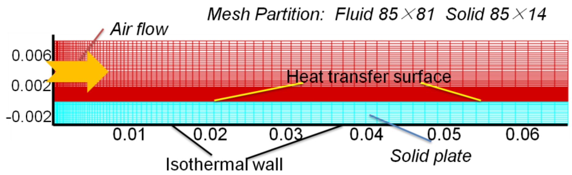
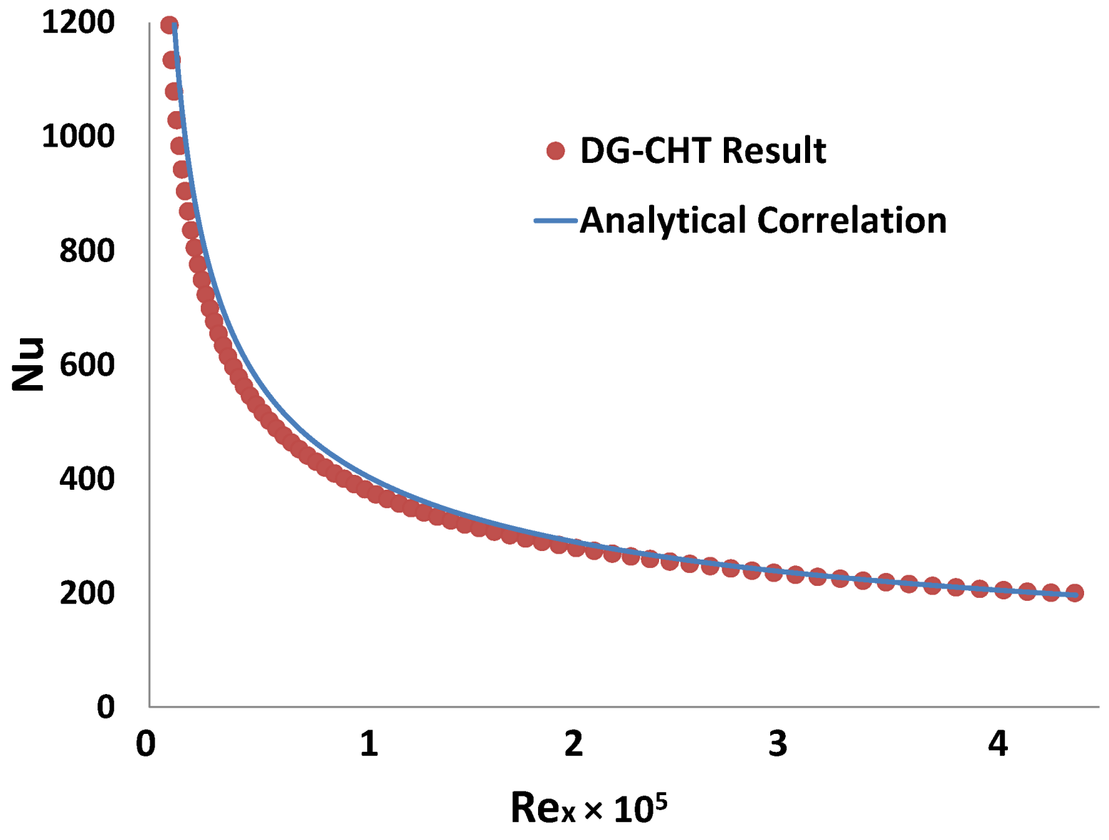
4.1. Heat Convection along a Flat Plate

The first case to validate the method presented in this paper is a 2-D simulation of the heat convection of laminar air flow with a total temperature of Tt_in = 328.97 K and total pressure of pt_in = 107.853 kPa, along a flat plate with the length of L = 66 mm and thickness of d = 3 mm, as showed in Figure 1. The isothermal condition T_b = 288.15 K is enforced on the bottom surface. The Reynolds and Mach numbers are Re_L = 4.4 × 10⁵ and Ma = 0.30. The mesh is devised to ensure more than 20 grid lines located inside the boundary layer region. Various kinds of solid materials are selected such that the thermal conductivity ratios of solid to fluid λ_s/λ_F range from 1 × 10¹ to 1 × 10⁴.

Figure 1. Computational domain and mesh for heat convection along a flat plate.

Figure 1. Computational domain and mesh for heat convection along a flat plate.

Figure 2 illustrates that under the method in this paper, the residual of temperature in the fluid domain can decrease nearly five orders of magnitude and that in the solid it can decrease over seven in this case. The chokes of decreasing residuals are conjectured to mainly originate from the lack of p-multigrid strategy in the available program, which may typically improve the convergence performance of DG formulations with natural or Taylor basis, although the residual minor oscillations in the results do not affect their reliability. Figure 3 shows that the temperature inside the solid has a tendency to the homogeneity with the increase of λ_f/λ_s, and the heat transfer surface also tends to the isothermal state. Figure 4 shows that when λ_f/λ_s ≈ 9 × 10³, the computed distribution of Nusselt number Nu = hL/λ_F along the surface is identical with the analytical correlation derived by Eckert and Weise [26].

Figure 2. The convergence curves of L²-norm of residuals (RMS) in the heat convection cases. (a) Aluminium (λ_f/λ_s ≈ 9 × 10³); (b) concrete (λ_f/λ_s ≈ 3 × 10¹).

Figure 2. The convergence curves of L²-norm of residuals (RMS) in the heat convection cases. (a) Aluminium (λ_f/λ_s ≈ 9 × 10³); (b) concrete (λ_f/λ_s ≈ 3 × 10¹).

Figure 3. Temperature contours inside the boundary layer and solid with different thermal conductivities.

Figure 3. Temperature contours inside the boundary layer and solid with different thermal conductivities.

Figure 4. Comparison of the computational and analytical Nusselt number when λ_s/λ_f≈ 9 × 10³.

Figure 4. Comparison of the computational and analytical Nusselt number when λ_s/λ_f≈ 9 × 10³.

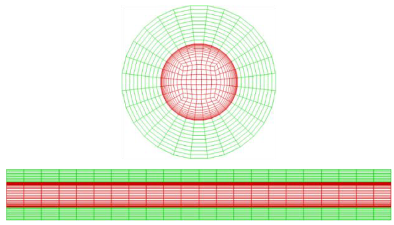
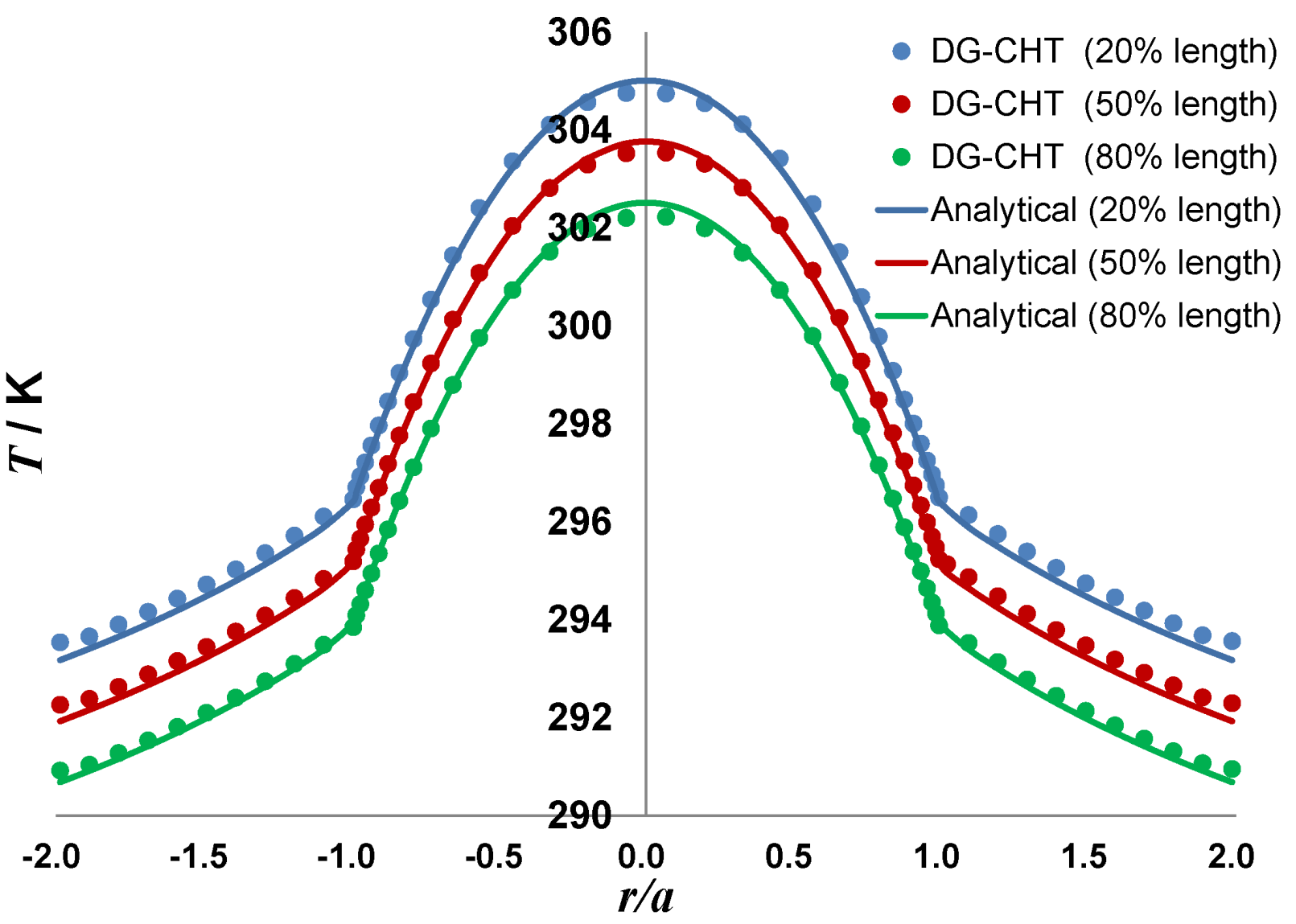
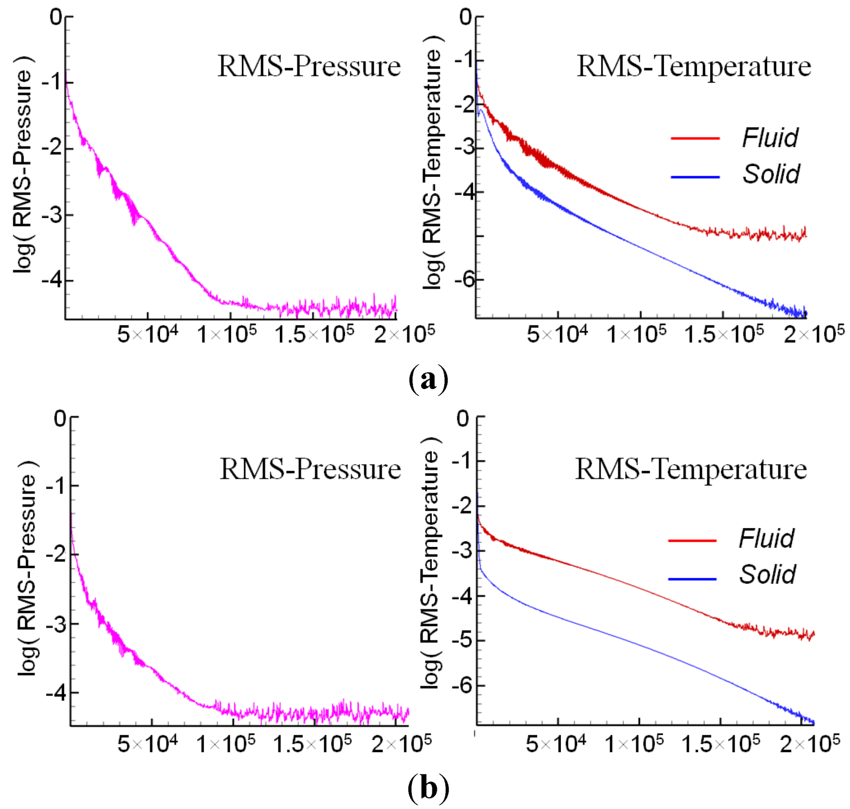
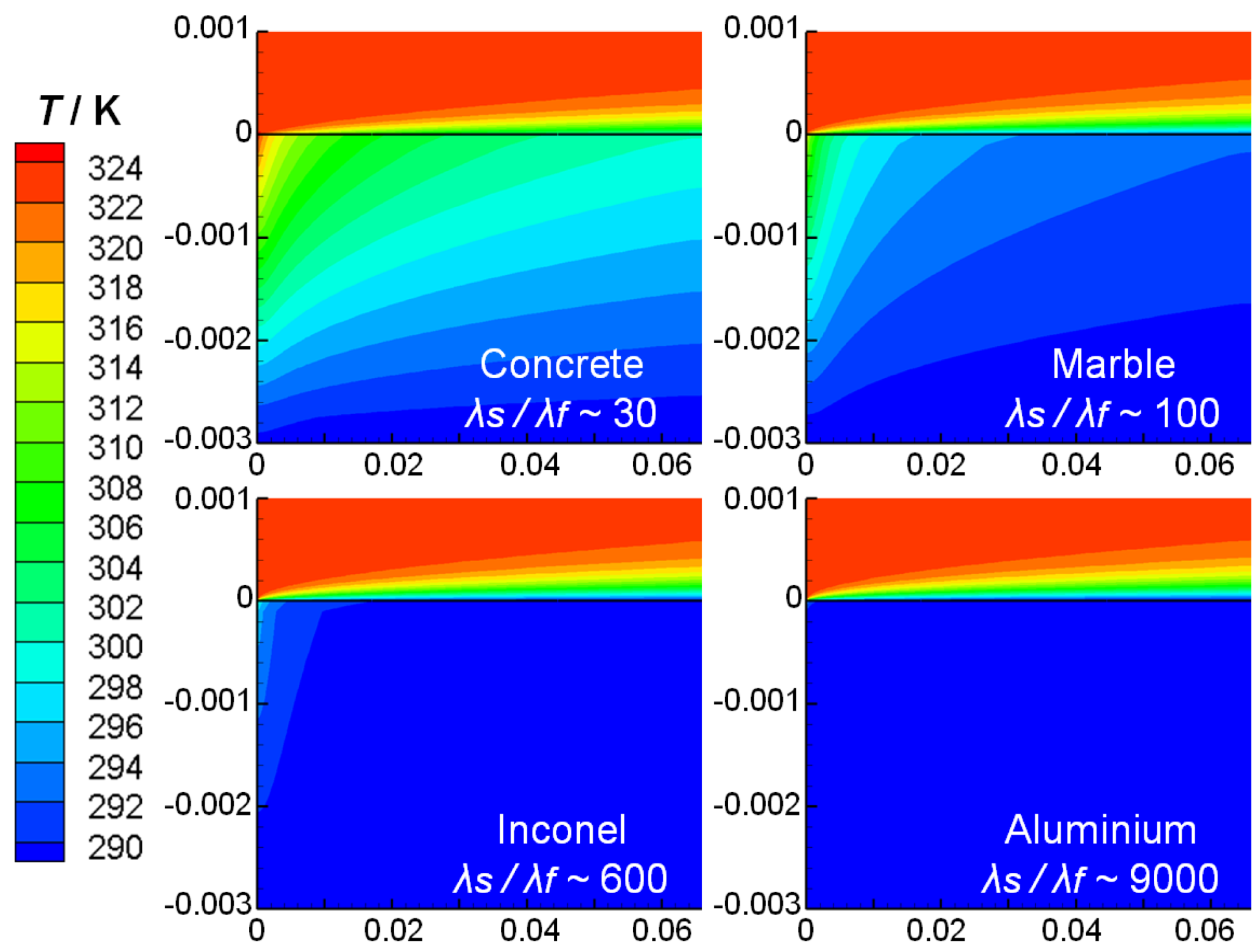
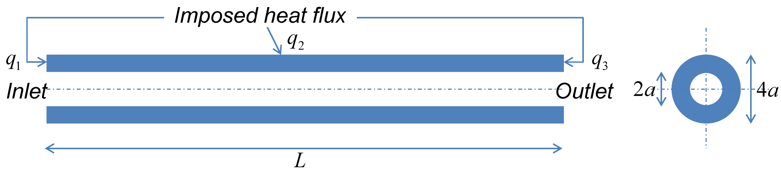
4.2. Heat Transfer of a Poiseuille Pipe Flow

The second case is the conjugate heat transfer of a Poiseuille pipe flow, of which the analytical solution was derived by Montenay et al. [2]. The geometry of the case is sketched in Figure 5. Air flows into a pipe with the length of L = 3 mm, inner diameter of 2a = 0.2 mm and outer diameter of 4a = 0.4 mm. The outer surface and both ends of the pipe are imposed heat flux q₁ = 138.5 W/m², q₂ = −2272 W/m² and q₃ = −138.5 W/m². The inlet static pressure is p_in = 102454 Pa and the static temperature is set to have the profile represented by the formula:

$$T_{\text{in}}=306\text{K}-\left(8.723\times {10}^8{\text{K/m}}^{\text{2}}\right)\cdot r^2$$

(30)

where r is the distance from a certain point to the pipe central line. The outlet condition is p_out = 100.00 kPa. The thermal conductivity is set to be λ_s = 0.1 W). According to our mesh independent study, the fluid and solid domains are partitioned into 8470 and 6160 elements respectively, as shown in Figure 6.

Figure 5. Geometry of the pipe flow case.

Figure 5. Geometry of the pipe flow case.

Figure 6. Computational domain and mesh of the pipe flow case.

Figure 6. Computational domain and mesh of the pipe flow case.

The computational temperature distributions at three different axial locations in Figure 7 appear as parabolic profiles in the fluid region and logarithmic profiles in the solid region, and also show good agreement with the analytical results in [2].

Figure 7. Comparison of temperature distributions of the pipe flow.

Figure 7. Comparison of temperature distributions of the pipe flow.

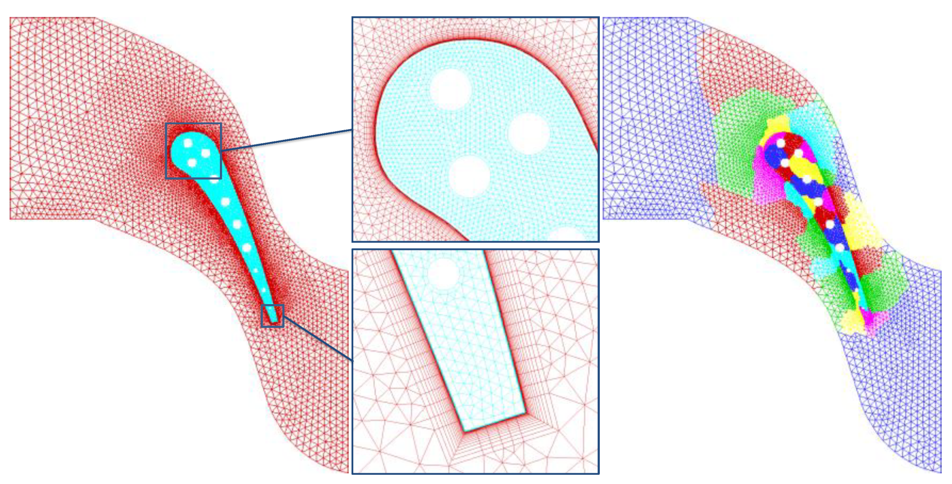
4.3. Application and analysis in a turbine vane

Here we take an application of the constructed platform in the simulation of a convection cooled high-pressure turbine nozzle guide vane named Mark II and analyze the numerical results. 2-D simulations of the condition #5411 (Table 1) in the experiment in [27] are carried out. The average temperatures of the cooling air and heat transfer coefficients of the inner cooling surfaces are given according to the experimental results (Table 2). ASTM 310 stainless steel is chosen to be the material of the vane in the simulation. According to the preparative mesh dependence study, we ultimately partition the fluid and solid regions into grids with the number of 18,597 and 6284, respectively, and with the type of mixed rectangular-triangle elements filled (Figure 8). The y⁺ value of the near wall gird is about 1.0. Figure 8 also shows the domain decomposition for the parallel computation. Different models including k-ω, BSL, SST and SST + γ-Re_θ are used to make a comparison of the results. The reference pressure is p_ref = pt_in = 337.080 kPa and the reference temperature is T_ref = 811 K.

Table 1. Test condition parameters of main flow for the case of the turbine vane Mark II.

Quantity	ptin	Tref	Tuin	pout
Unit	kPa	K	%	kPa
Value	337.080	788.0	6.5	169.849

Table 1. Test condition parameters of main flow for the case of the turbine vane Mark II.

Quantity	ptin	Tref	Tuin	pout
Unit	kPa	K	%	kPa
Value	337.080	788.0	6.5	169.849

Table 2. Test condition parameters of inner holes boundaries for the case of the turbine vane Mark II.

Hole index	Average temperature of cooing air (K)	Average heat transfer coefficient (W/m2·K)
01	336.39	1943.67
02	326.27	1881.45
03	332.68	1893.49
04	338.86	1960.62
05	318.95	1850.77
06	315.58	1813.36
07	326.26	1871.88
08	359.83	2643.07
09	360.89	1809.89
10	414.85	3056.69

Table 2. Test condition parameters of inner holes boundaries for the case of the turbine vane Mark II.

Hole index	Average temperature of cooing air (K)	Average heat transfer coefficient (W/m2·K)
01	336.39	1943.67
02	326.27	1881.45
03	332.68	1893.49
04	338.86	1960.62
05	318.95	1850.77
06	315.58	1813.36
07	326.26	1871.88
08	359.83	2643.07
09	360.89	1809.89
10	414.85	3056.69

Figure 8. Mesh partition and succedent domain decomposition (into 32 subdomains) processes for the case of the turbine vane Mark II.

Figure 8. Mesh partition and succedent domain decomposition (into 32 subdomains) processes for the case of the turbine vane Mark II.

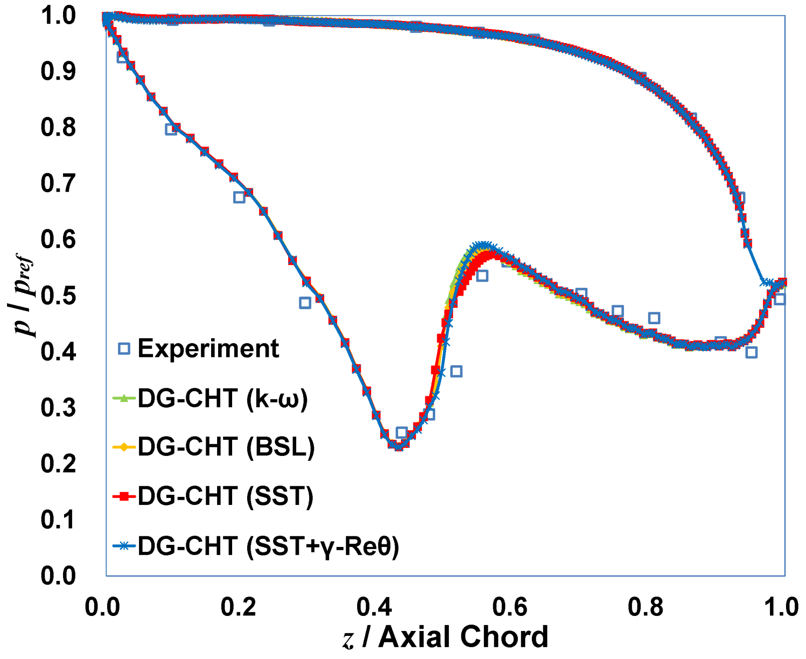
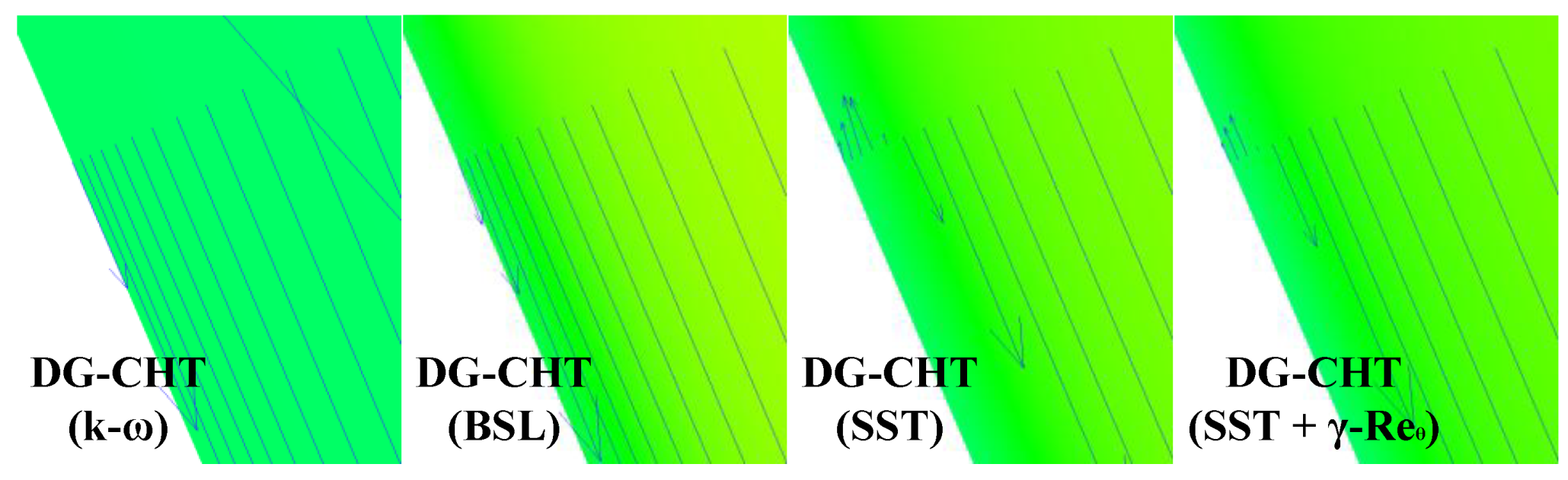
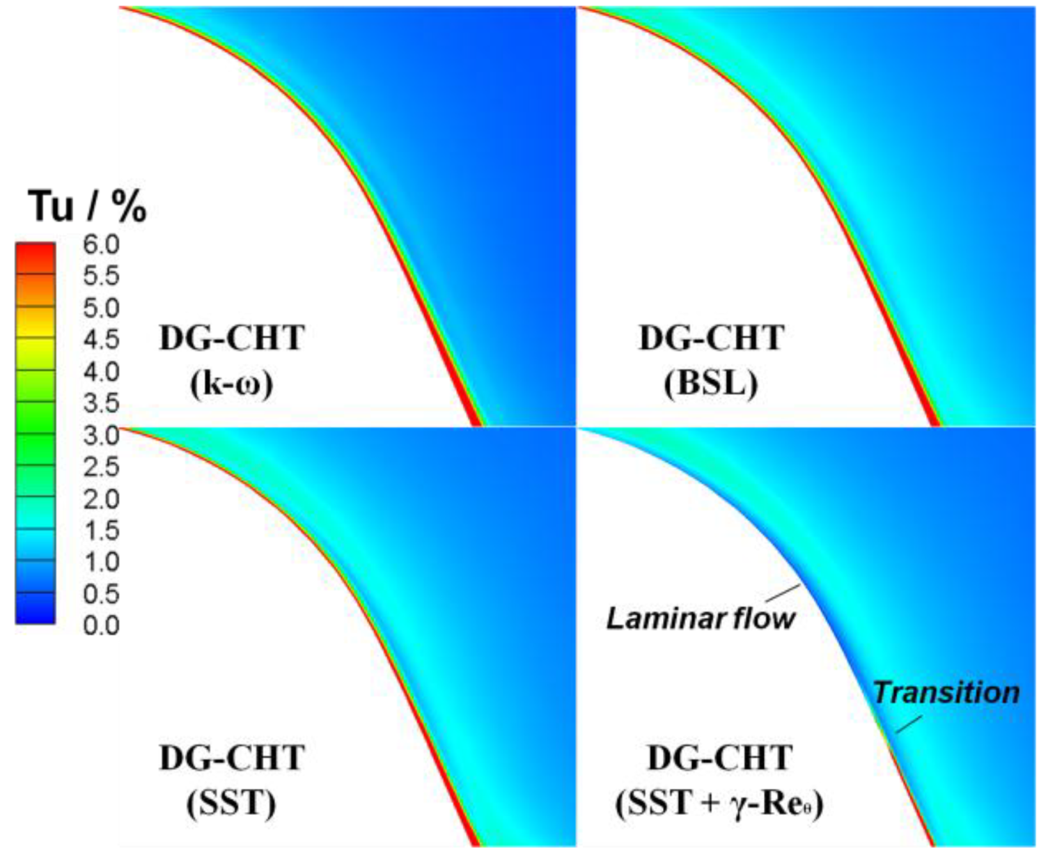
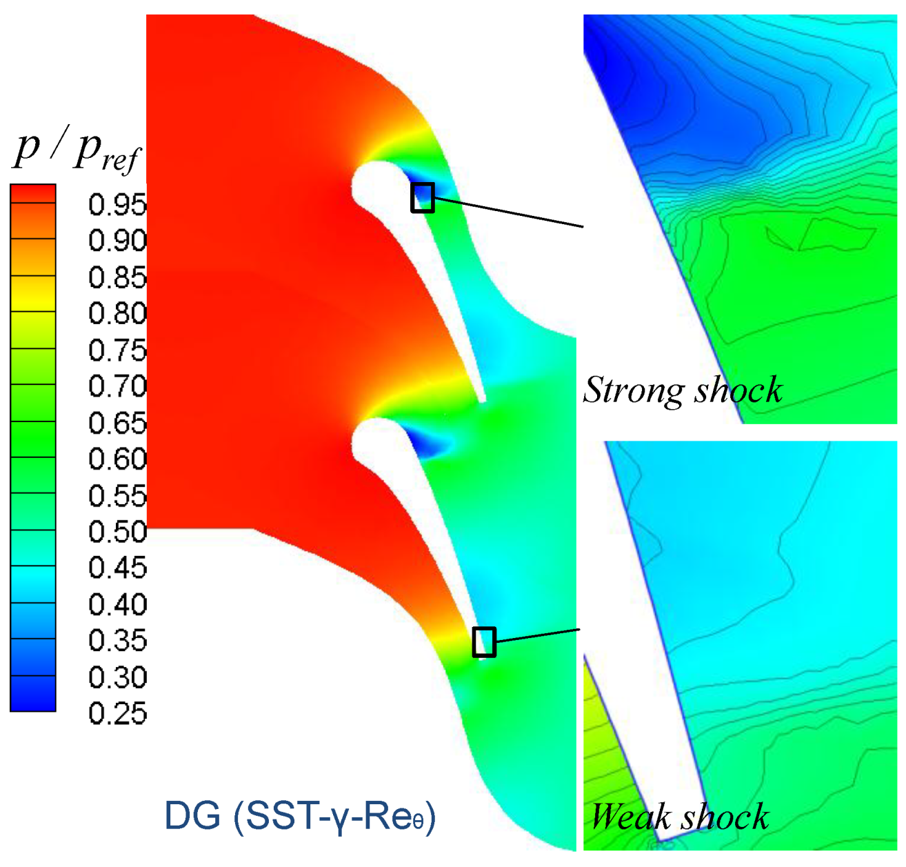
4.3.1. Aerodynamic Features

All the numerical models predict very similar aerodynamic performance illustrated by the good agreements between computed and experimental surface pressure distributions shown in Figure 9. On the suction side, the flow accelerates around the leading edge and forms a strong shock at the location at about a half of the axial chord. It accelerates again to supersonic downstream of the strong shock, and forms the second, relatively weak shock near the trailing edge. On the pressure side, the flow gently accelerates in general. Figure 10 shows the pressure contour and isolines around the shock regions, giving a visualized observation of the computed aerodynamic characteristics. The velocity vectors in Figure 11 illustrate that the shock-induced separation occurs behind the strong shock near suction surface in the results of SST and SST + γ-Re_θ models but doesn’t in those of k-ω and BSL models. The distinction mainly stems from the fact that the SST model adopts the Bradshaw assumption [28] to decrease the computed Reynolds shear stress inside boundary layer and consequently enhance the trend of its separation under adverse pressure gradient.

Figure 9. Pressure distributions on the vane surface.

Figure 9. Pressure distributions on the vane surface.

Figure 10. Computed pressure contour of Mark II (SST + γ-Re_θ).

Figure 10. Computed pressure contour of Mark II (SST + γ-Re_θ).

Figure 11. Near-wall velocity vectors just behind the strong shock wave.

Figure 11. Near-wall velocity vectors just behind the strong shock wave.

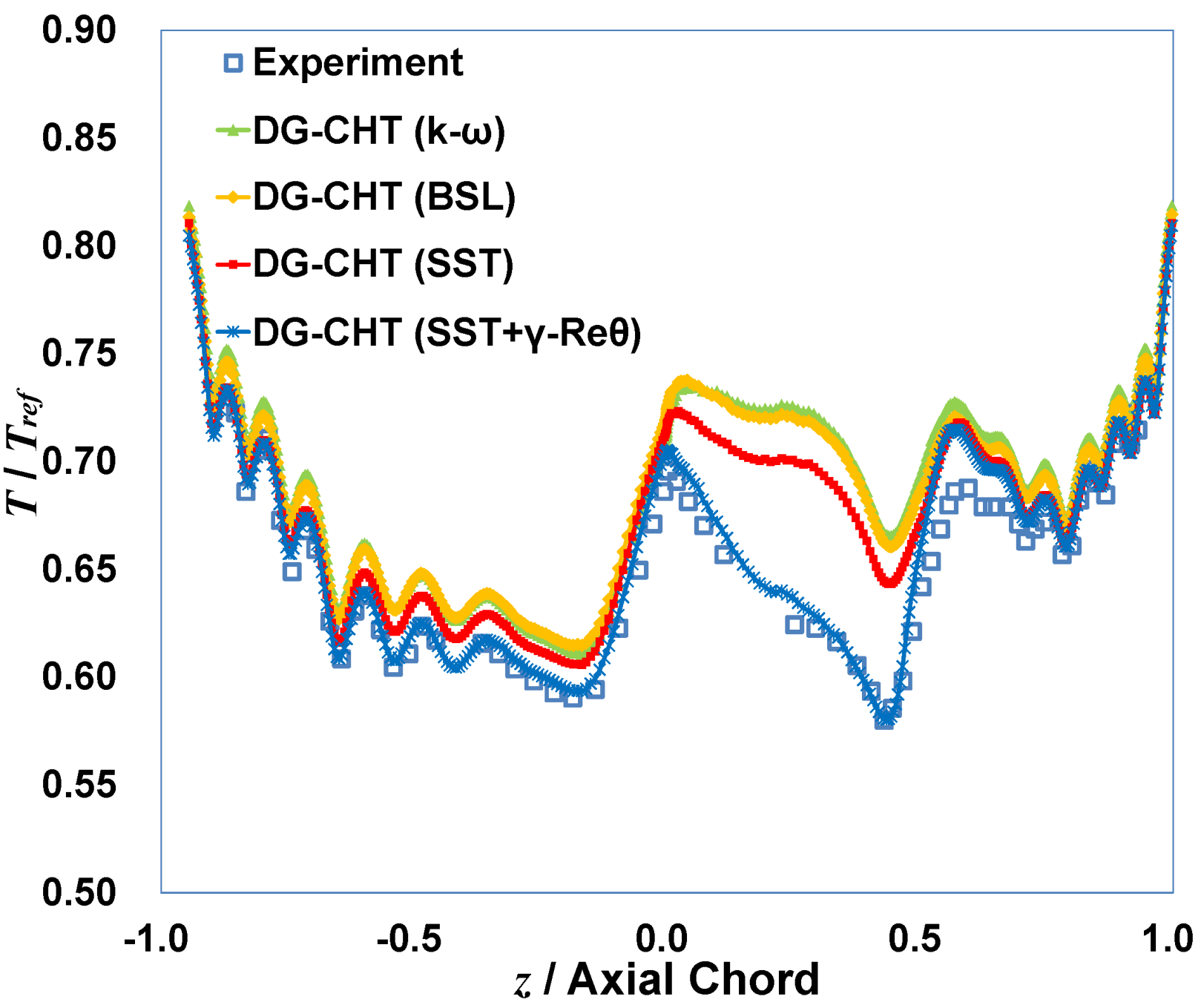
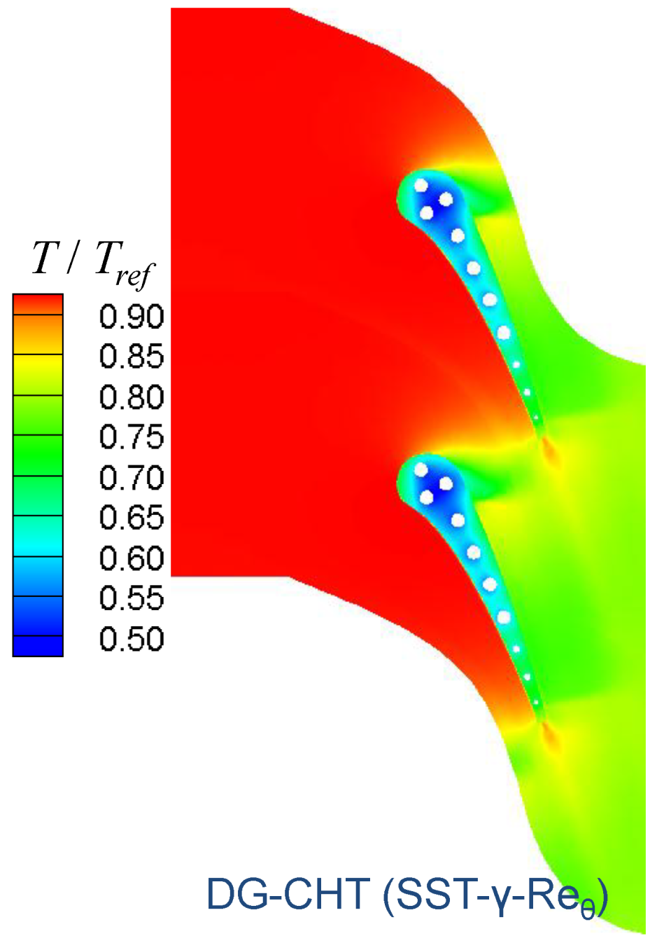
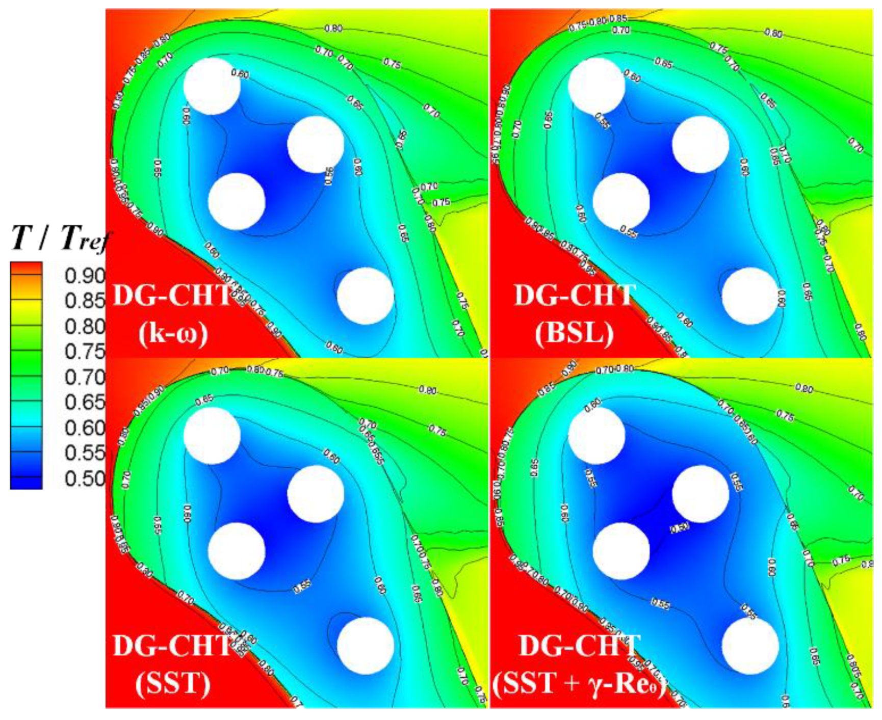
4.3.2. Heat Transfer Features

The comparison of computed and experimental results of vane surface temperature distributions is illustrated in Figure 12. All the results indicate that on the suction side, the surface temperature reaches a local maximum at the stagnation point around the leading edge and then decreases due to the flow acceleration and the cooling effects of the first three channels. It rises sharply when traversing the strong shock. Behind the shock, the surface temperature appears a rising tendency with fluctuations due to the decrease of the vane thickness and the discrete cooling channels. On the pressure side, the minimum of surface temperature exists at the inflection point of the vane profile and then appears a similar tendency with the suction side. Figure 13 shows the temperature contour in the flow passage and inside the vane.

Figure 12. Temperature distributions on the vane surface.

Figure 12. Temperature distributions on the vane surface.

Figure 13. Computed temperature contour of Mark II (SST + γ-Re_θ).

Figure 13. Computed temperature contour of Mark II (SST + γ-Re_θ).

From Figure 12 we can observe the result of the SST + γ-Re_θ model has the best agreement with the experimental one in general, especially in the region from the stagnation point to the strong shock on the suction surface. A more detailed observation is shown in Figure 14 which illustrates that in this region the boundary layer appears to have much lower turbulence intensity predicted by SST + γ-Re_θ model than the other three (k-ω, BSL, and SST), and the transition to turbulence occurs near the end of this region due to strong deceleration induced by the shock. The laminar region existing in the result of SST + γ-Re_θ model makes the computed surface thermal resistance larger than the ones of the other models, and leads to lower (so closer to the real) temperature on the surface and also inside the vane (as in Figure 15). The comparison above implies that numerical models containing no reasonable modes to predict transitions may do not have the potential to precisely simulate this kind of heat transfer problem.

Figure 14. Turbulence intensity contours in the boundary layers above the suction surface around leading edge of the vane.

Figure 14. Turbulence intensity contours in the boundary layers above the suction surface around leading edge of the vane.

Figure 15. Temperature contours around leading edge of the vane.

Figure 15. Temperature contours around leading edge of the vane.

Figure 12 also indicates that all the models overestimate the surface temperature just behind the strong shock. The deviation is conjectured to result from the overestimation of turbulence intensity inside the boundary layer behind the shock. In fact, most two-equation turbulence models without compressibility corrections predict excessive turbulence kinetic energy behind shocks [29]. Moreover, since the transition process is triggered around the shock region concurrently, an alternative reason of the temperature deviation for SST + γ-Re_θ model may be that the start of full turbulent boundary layer (i.e., the end of the transition process) predicted by the γ-Re_θ model is located upstream of the real one, partially due to the model’s overlook of the compressible effects on the transition onset and length. The fact that the compressibility can defer the transition onset and increase its length has been realized by some researches (e.g., [30,31]), although complete experimental correlations as a function of Mach number haven’t been established entirely. So both turbulence and transition models considering compressible effects are worth exploring in the future.

5. Conclusions

In this paper, we have presented a primary framework for the simulation of CHT using DG methods on unstructured grids, and a corresponding simulation platform fit for general engineering problems in gas turbines is developed. The centroid-expanded Taylor basis is adopted for various element types. The Bassi-Rebay method is used in the gradient computation inside both fluid and solid domains. A strategy for data exchange through the fluid-solid interface based on the numerical flux of quadrature points is devised to enforce the fully coupled implementation.

The compressible RANS equations combined with turbulence and transition modeling equations, and the heat conduction Fourier’s equation, are solved under the unified DG algorithm to realize the applications of the advanced numerical models and algorithm in CHT simulations. An approximate implicit treatment of the source terms in k-ω/BSL/SST models, with the turbulence frequency transportation represented by its logarithm, is derived to decrease the adverse impact rooted in the source term stiffness and make them more compatible with the entire explicit framework.

Some cases were studied to validate the feasibility of the method as well as the numerical platform developed. In its application on Mark II, the result of the code combined with the SST + γ-Re_θ model showed very good agreement with the experiment for both aerodynamic and heat transfer features. The numerical reasons of the general overestimation of surface temperature just behind the shock were conjectured to mainly result from the ignorance of the compressibility for both the turbulence models and the transition model based on experiment calibration with low Mach number.

The expected advantages of DG methods in the CHT simulations compared with the traditional FV methods, as briefly analyzed in the first section in this paper, need to be further investigated and confirmed, especially when elements with poor quality or non-conformable elements are used near the interface. In addition, more efficient time integration methods will be considered to alleviate the huge computational cost of the DG methods (the computational time consumed by the available explicit DG program was usually about one order of magnitude higher than the FV-based commercial software for these cases). The present work can be viewed as a first attempt towards further investigations of DG and other high-accuracy methods’ applications in the engineering CHT problems where their superiority can be seen.

References

1. Martin, T.J.; Dulikravich, G.; Han, Z.-X.; Dennis, B.H. Minimization of coolant mass flow rate in internally cooled gas turbine blades. In Proceedings of the ASME Turbo Expo, Indianapolis, IN, USA, 7–10 June 1999.
2. Montenay, A.; Pate, L.; Duboue, J. Conjugate heat transfer analysis of an engine internal cavity. In Proceedings of the ASME Turbo Expo 2000: Power for Land, Sea, and Air, Munich, Germany, 8–11 May 2000.
3. Sondak, D.L.; Dorney, D.J. Simulation of coupled unsteady flow and heat conduction in turbine stage. J. Propuls. Power 2000, 16, 1141–1148. [Google Scholar] [CrossRef]
4. Verdicchio, J.; Chew, J.; Hills, N. Coupled fluid/solid heat transfer computation for turbine discs. In Proceedings of the ASME Turbo Expo 2001: Power for Land, Sea, and Air, New Orleans, LA, USA, 4–7 June 2001; Volume 3.
5. Duchaine, F.; Mendez, S.; Nicoud, F.; Corpron, A.; Moureau, V.; Poinsot, T. Coupling heat transfer solvers and large eddy simulations for combustion applications. In Proceedings of the Summer Program, Stanford, CA, USA, 6 July–1 August 2008; pp. 113–126.
6. Amaral, S.; Verstraete, T.; van den Braembussche, R.; Arts, T. Design and optimization of the internal cooling channels of a HP turbine blade: Part 1—Methodology. In Proceedings of the American Society of Mechanical Engineers (ASME) Turbo Expo 2008: Power for Land, Sea, and Air, Berlin, Germany, 9–13 June 2008.
7. Pelletier, D.; Ignat, L.; Ilinca, F. Adaptive finite element method for conjugate heattransfer. Numer. Heat Trans. Part A Appl. 1997, 32, 267–287. [Google Scholar] [CrossRef]
8. Kao, K.-H.; Liou, M.-S. Application of chimera/unstructured hybrid grids for conjugate heat transfer. AIAA J. 1997, 35, 1472–1478. [Google Scholar] [CrossRef]
9. Han, Z.-X.; Dennis, B.H.; Dulikravich, G.S. Simultaneous prediction of external flow-field and temperature in internally cooled 3-D turbine blade material. Int. J. Turbo Jet Engines 2000, 18, 47–58. [Google Scholar]
10. Agostini, F.; Arts, T. Conjugate heat transfer investigation of rib-roughened cooling channels. In Proceedings of the ASME Turbo Expo 2005: Power for Land, Sea, and Air, Reno, NV, USA, 6–9 June 2005; Volume 3, pp. 239–247.
11. Luo, J.; Razinsky, E.H. Conjugate heat transfer analysis of a cooled turbine vane using the V2F turbulence model. J. Turbomach. 2007, 129, 773–781. [Google Scholar] [CrossRef]
12. Reed, W.; Hill, T. Triangular Mesh Methods for the Neutron Transport Equation; Technical Report LA-UR-73-479; Los Alamos Scientific Laboratory: Los Alamos, NM, USA, 1973. [Google Scholar]
13. Cockburn, B.; Shu, C.-W. TVB Runge-Kutta local projection discontinuous Galerkin finite element method for conservation laws. II. General framework. Math. Comput. 1989, 52, 411–435. [Google Scholar]
14. Cockburn, B.; Lin, S.-Y.; Shu, C.-W. TVB Runge-Kutta local projection discontinuous Galerkin finite element method for conservation laws III: One-dimensional systems. J. Comput. Phys. 1989, 84, 90–113. [Google Scholar] [CrossRef]
15. Cockburn, B.; Hou, S.; Shu, C.-W. The Runge-Kutta local projection discontinuous Galerkin finite element method for conservation laws. IV. The multidimensional case. Math. Comput. 1990, 54, 545–581. [Google Scholar]
16. Cockburn, B.; Shu, C.-W. The Runge-Kutta discontinuous Galerkin method for conservation laws V: Multidimensional systems. J. Comput. Phys. 1998, 141, 199–224. [Google Scholar] [CrossRef]
17. Bassi, F.; Rebay, S. A high-order accurate discontinuous finite element method for the numerical solution of the compressible Navier-stokes equations. J. Comput. Phys. 1997, 131, 267–279. [Google Scholar] [CrossRef]
18. Bassi, F.; Crivellini, A.; Rebay, S.; Savini, M. Discontinuous Galerkin solution of the Reynolds-averaged Navier-Stokes and k-ω turbulence model equations. Comput. Fluids 2005, 34, 507–540. [Google Scholar] [CrossRef]
19. Kanapady, R.; Jain, A.; Tamma, K.; Siddharth, S. Local discontinuous Galerkin formulations for heat conduction problems involving high gradients and imperfect contact surfaces. In Proceedings of the 43rd AIAA Aerospace Sciences Meeting and Exhibit, Reno, NV, USA, 10–13 January 2005; pp. 8447–8455.
20. Menter, F.; Langtry, R.; Likki, S.; Suzen, Y.; Huang, P.; Volker, S. A correlation-based transition model using local variables—Part I: Model formulation. J. Turbomach. 2006, 128, 413–422. [Google Scholar] [CrossRef]
21. Langtry, R.B.; Menter, F.R. Correlation-based transition modeling for unstructured parallelized computational fluid dynamics codes. AIAA J. 2009, 47, 2894–2906. [Google Scholar] [CrossRef]
22. Li, X.-S.; Gu, C.-W. An all-speed roe-type scheme and its asymptotic analysis of low Mach number behaviour. J. Comput. Phys. 2008, 227, 5144–5159. [Google Scholar] [CrossRef]
23. Wilcox, D.C. Reassessment of the scale-determining equation for advanced turbulence models. AIAA J. 1988, 26, 1299–1310. [Google Scholar] [CrossRef]
24. Menter, F.R. Two-equation eddy-viscosity turbulence models for engineering applications. AIAA J. 1994, 32, 1598–1605. [Google Scholar] [CrossRef]
25. Kuzmin, D. A vertex-based hierarchical slope limiter for p-adaptive discontinuous Galerkin methods. J. Comput. Appl. Math. 2010, 233, 3077–3085. [Google Scholar] [CrossRef]
26. Eckert, E.; Weise, W. Die temperatur unbeheizter Koerper in einem Gasstrom hoher Geschwindigkeit. Forsch. Geb. Ing. A. 1941, 12, 40–50. (In German) [Google Scholar] [CrossRef]
27. Hylton, L.; Mihelc, M.; Turner, E.; Nealy, D.; York, R. Analytical and Experimental Evaluation of the Heat Transfer Distribution over the Surfaces of Turbine Vanes; Technical Report for the National Aeronautics and Space Administration (NASA): Indianapolis, IN, USA, 1 May 1983. [Google Scholar]
28. Bradshaw, P.; Ferriss, D.; Atwell, N. Calculation of boundary layer development using the turbulent energy equation. J. Fluid Mech. 1967, 28, 593–616. [Google Scholar] [CrossRef]
29. Coakley, T.; Huang, P. Turbulence modeling for high speed flows. In Proceedings of the AIAA 30th Aerospace Sciences Meeting, Reno, NV, USA, 6–9 January 1992.
30. Bovle, R.; Simon, F. Mach number effects on turbine blade transition length prediction. J. Turbomach. 1999, 121, 694–702. [Google Scholar] [CrossRef]
31. Steelant, J.; Dick, E. Modeling of laminar-turbulent transition for high freestream turbulence. J. Fluids Eng. 2001, 123, 22–30. [Google Scholar] [CrossRef]