1. Introduction
For a horizontal-axis wind turbine (HAWT) system, the efficiency of the system transformation is related to the blade shape. Therefore it is critical to design the most efficient blade shape possible. Blade element momentum (BEM) theory is widely used when designing a HAWT blade shape and predicts its performance using a fairly simple procedure [
1]. This theory requires combining the two-dimensional (2D) airfoil data to obtain the optimum blade shape, including the distributions of chord length and the twist angle along the span-wise direction. It should be noted that the optimization of a HAWT blade is done at the design tip speed ratio (λ
d) and the design angle of attack (α
D). In other words, if the optimal blade is operated at a different tip speed ratio than the one for which it has been designed, it will no longer be optimal [
1,
2]. However, for this paper the performances of the blade are tested for the entire range between the tip speed ratios of 0 and 9. In past research, analysis focused only on the optimal blade shape within a constant-speed operation system [
3,
4,
5]. The purpose of this study is to construct a HAWT system with variable-speed operation in which the optimum blade is determined using BEM theory. For comparative purposes, two other blades are also considered, as will be discussed later.
In general, three methods may be used to analyze the performance of HAWT blades. The first one is the improved BEM model, as performed by Bai
et al. [
6] and this model can quickly predict the blade performance. This improved BEM model includes two modifications that can greatly increase the accuracy for the blade performance curve prediction: tip-loss factor by Prandtl [
7] and the stall delay model [
8,
9]. The second method is to experiment in a wind tunnel. For instances, Hirahara
et al. [
10] and Koki
et al. [
11] propose using the similitude method by measuring the mechanical torque generated by the blade using a small-scale wind turbine system. Both papers use a torque transducer installed on the shaft between the blade and the generator to measure the mechanical torque. Hirahara
et al. [
10] applied an electronic load to change the rotational speed of the rotor blade to obtain performance curves. This technique has been successfully applied to a 500 mm diameter 4-blade HAWT system that ran at a rated rotational speed of 1500 rpm and a rated wind speed of 12 m/s.
Here, the power coefficient (
Cp), which is the efficiency transferred from the blade, was successfully calculated using a torque transducer. In addition, it was found that both the generator’s efficiency and the system’s total efficiency can be determined in this wind tunnel experiment. In a previous experiment, Koki
et al. [
11] used BEM theory to verify and compare the results with the performance curves of a wind tunnel experiment and found that BEM is a good method for predicting the blade performance. Finally, Computational Fluid Dynamic (CFD) is a good method for analyzing and verifying the performance of different types of blade shapes. For example, the National Aerospace Laboratory successfully developed a wind turbine with a 500 kW, low-cost, horizontal-axis, downwind, teetered and stall regulated two-bladed model using the CFD method to consider the optimum blade design and performance analysis [
12]. Tachos,
etc. [
13] have used the Reynolds averaged Navier-Stokes equations combined with the
k-
ω SST turbulence model that describes the three dimensional (3D) steady state flow around the blade solved with the aid of a commercial CFD code for computing the aerodynamic characteristics of the NREL Phase VI rotor blade which is a horizontal-axis downwind turbine rotor [
5,
14].
2. Brief Description of the BEM Method
The aerodynamic curves of the 2D airfoil are needed to analyze and combined these curves with the BEM theory to design the optimal blade shape. In this study, we obtained the NACA4418 airfoil data for BEM calculation by using the freeware XFoil from Massachusetts Institute of Technology [
15]. From
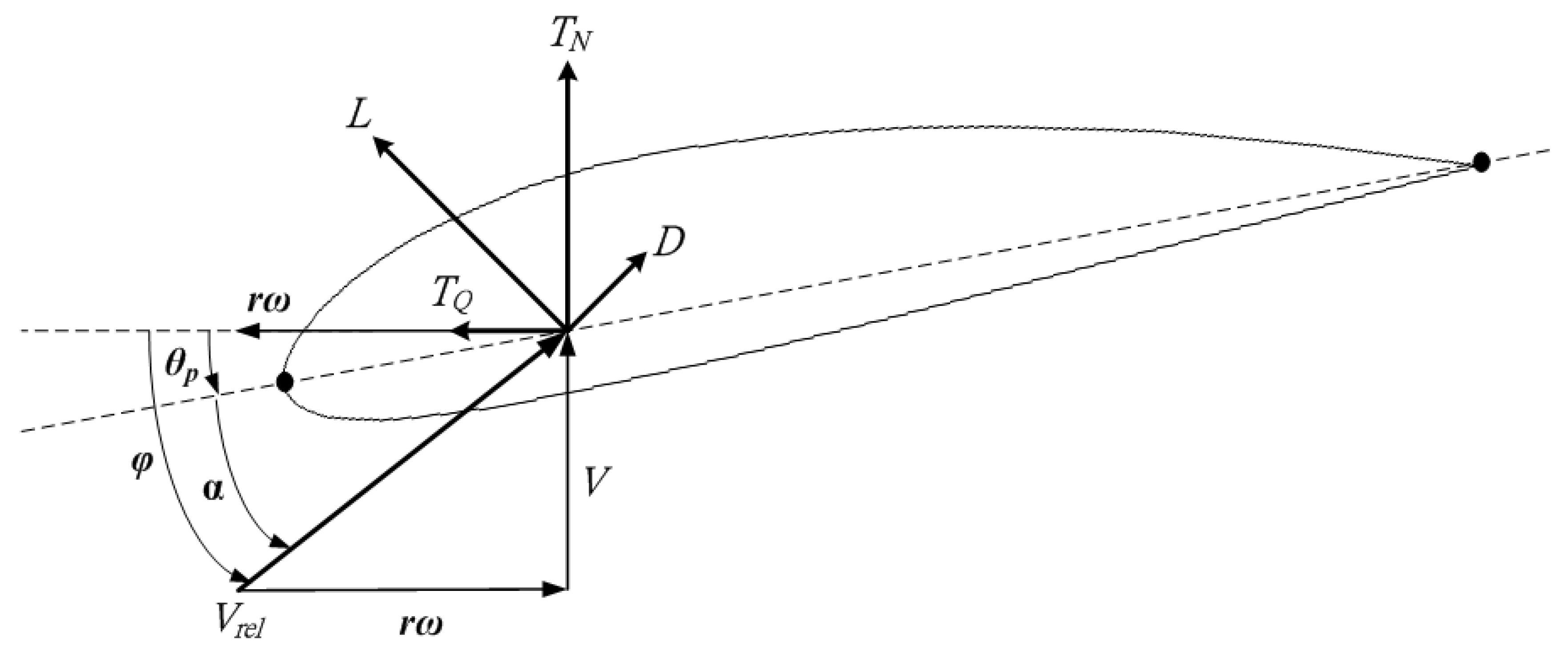
Figure 1, it can be seen that it is possible to obtain the distribution of the angle of relative wind (
φ) which consists of pitch angle (
θp), twist angle (β) and angle of attack (α) on one of the blade sections (airfoil) by employing BEM theory [
1,
2,
6].
Figure 1 also shows the forces acting on an airfoil section, where
TN is defined as the thrust and
TQ is defined as the torque. Both are generated by lift (
L) and drag (
D) forces. The lift and drag are available as functions of the angle of attack and the Reynolds number (
Re) which is defined as:
where
cavg. is the average chord length of each blade section;
ρ is the air density;
μ is the kinematic viscosity; and
Vrel is the relative wind speed which consists of wind speed (
V) and rotational speed (
ω).
Figure 1.
Diagram of angles and forces on one of the blade section.
Figure 1.
Diagram of angles and forces on one of the blade section.
The blade shape used in this paper is a NACA4418 airfoils set with a design angle of attack (α
D) of 5.5°.
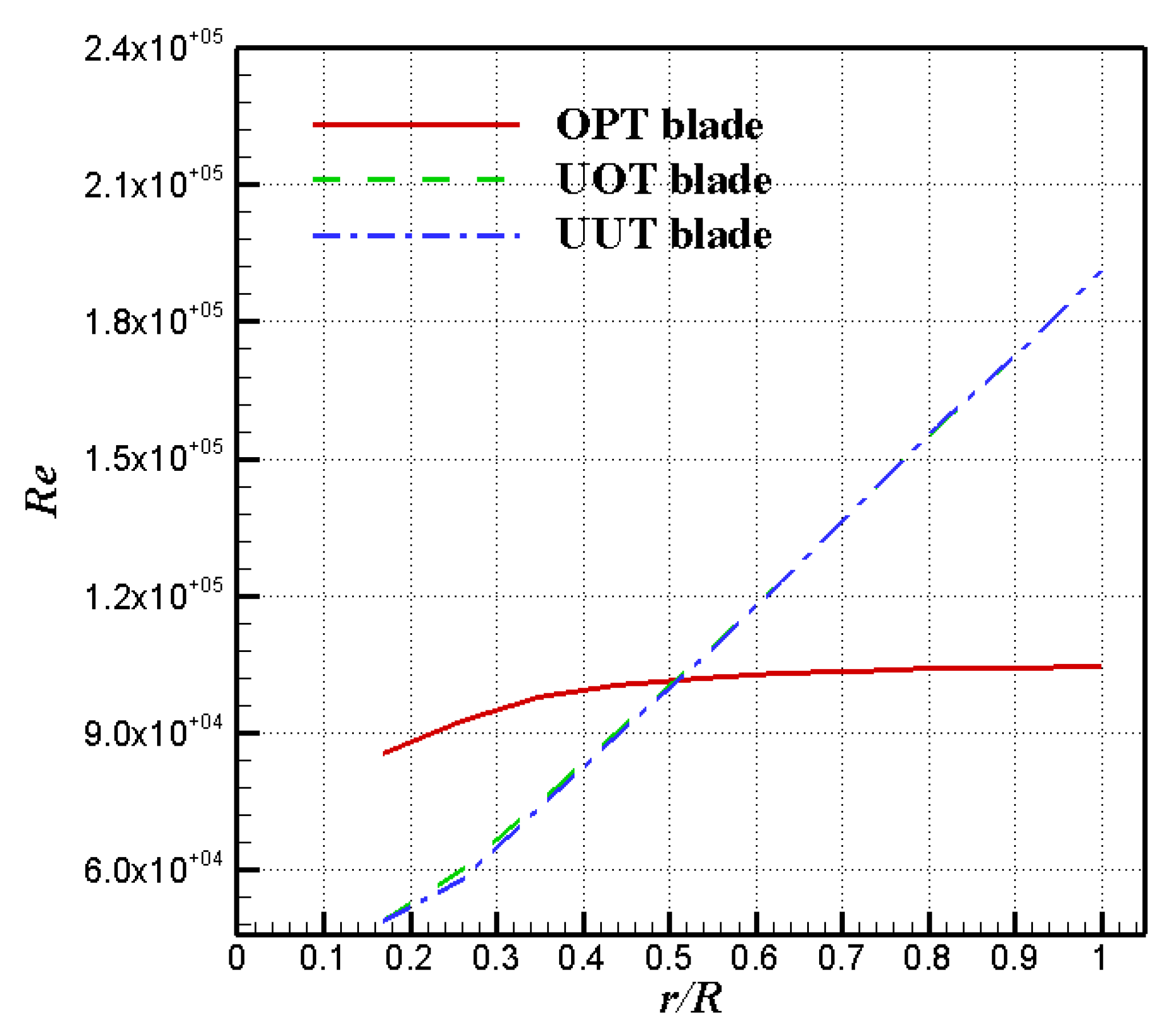
Figure 2 shows the distribution of Reynolds numbers in each section at a wind speed of 10 m/s and tip speed ratio of 5 for the tested blade models used in the following content. We can see the distributions of Reynolds numbers of the OPT blade are between 8.0 × 10
4 and 1.1 × 10
5; there is very little difference in the root region (
r/
R = 0.2–0.4) for the UOT and UUT blades. For this reason, a Reynolds number of 1.0 × 10
5 has been selected for the XFoil software calculation, which results in a lift coefficient (
Cl) of 0.9005 and a lift to drag ratio (
Cl/
Cd) of 48. From
Figure 2 it can be seen that the distributions of Reynolds number in the tested models are between 6.0 × 10
4 and 2.0 × 10
5 and the effect of the transition flow could occur in this case that caused from laminar to turbulence flow. The transition flow in XFoil relies on the e
n method, which has a user-specified parameter called the transition amplification ratio,
Ncrit, which is the log of the amplification of the most-amplified frequency. Thus, the transition amplification ratio,
Ncrit, has been set to 1 in XFoil [
15] which was used in order to simulate both the effects of a wind tunnel free-stream turbulence intensity and blade surface roughness [
15].
Figure 2.
The distributions of Reynolds number in each section at V = 10 m/s and λ = 5.
Figure 2.
The distributions of Reynolds number in each section at V = 10 m/s and λ = 5.
The normalized parameter for tip speed ratio (λ) is defined as:
where
R is the radius of the blade. The test range of λ in this study is restricted between 2 and 9. In a steady state test, such as wind tunnel experiment, the distributions of angle of attack and Reynolds number can be changed with the various tip speed ratios, which will vary with the rotational speed.
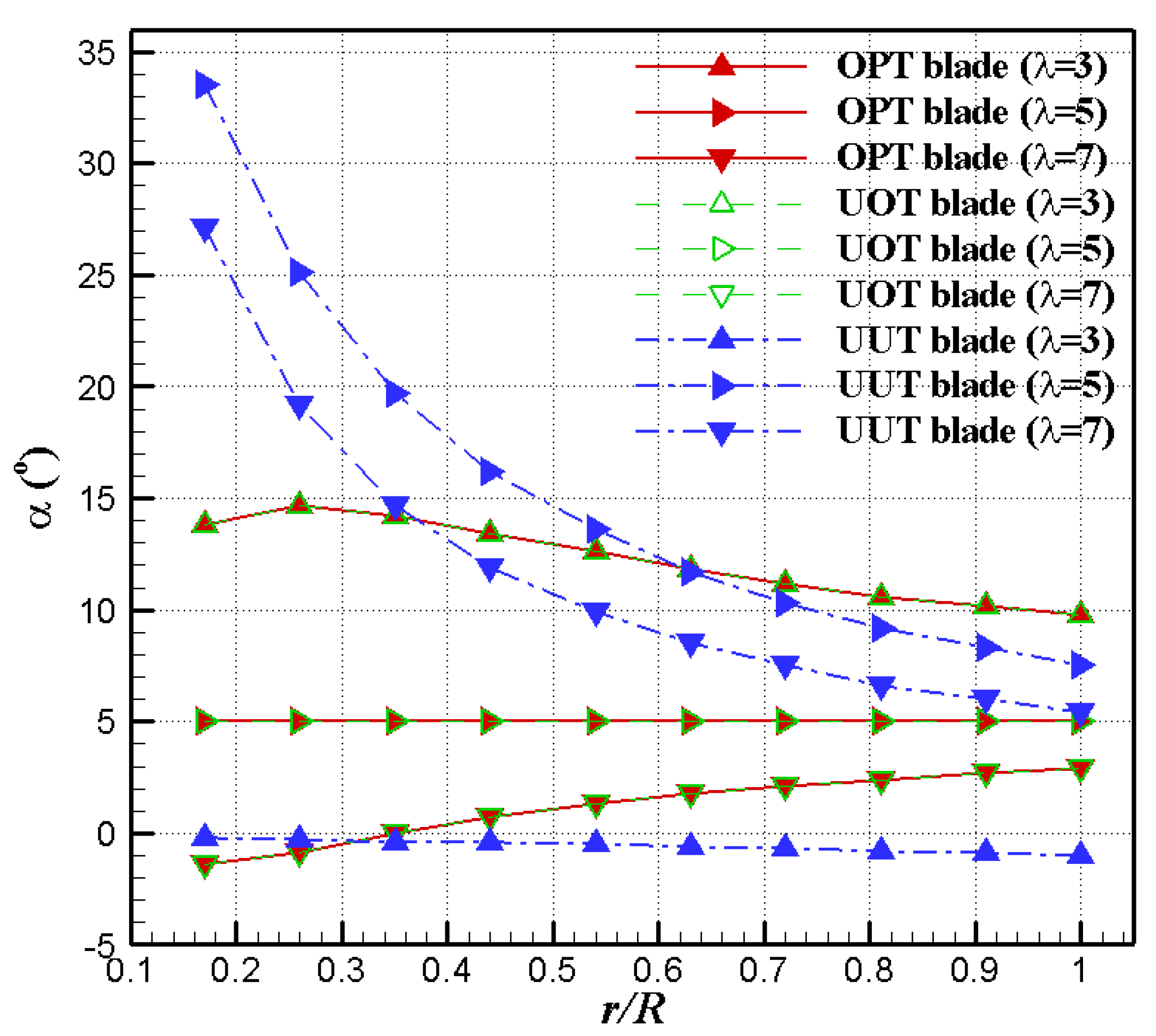
Figure 3 shows the distributions of angle of attack along each section at a wind speed of 10 m/s and tip speed ratios of 3, 5 and 7 for the tested models. Obviously, the distributions of angle of attack in each section between OPT and UOT blades completely overlap, because they have the same pitch angles but different chord length distributions in each section. Because the rotational speed of the blade influences the Reynolds number, it is necessary to check its influence over this lift and drag.
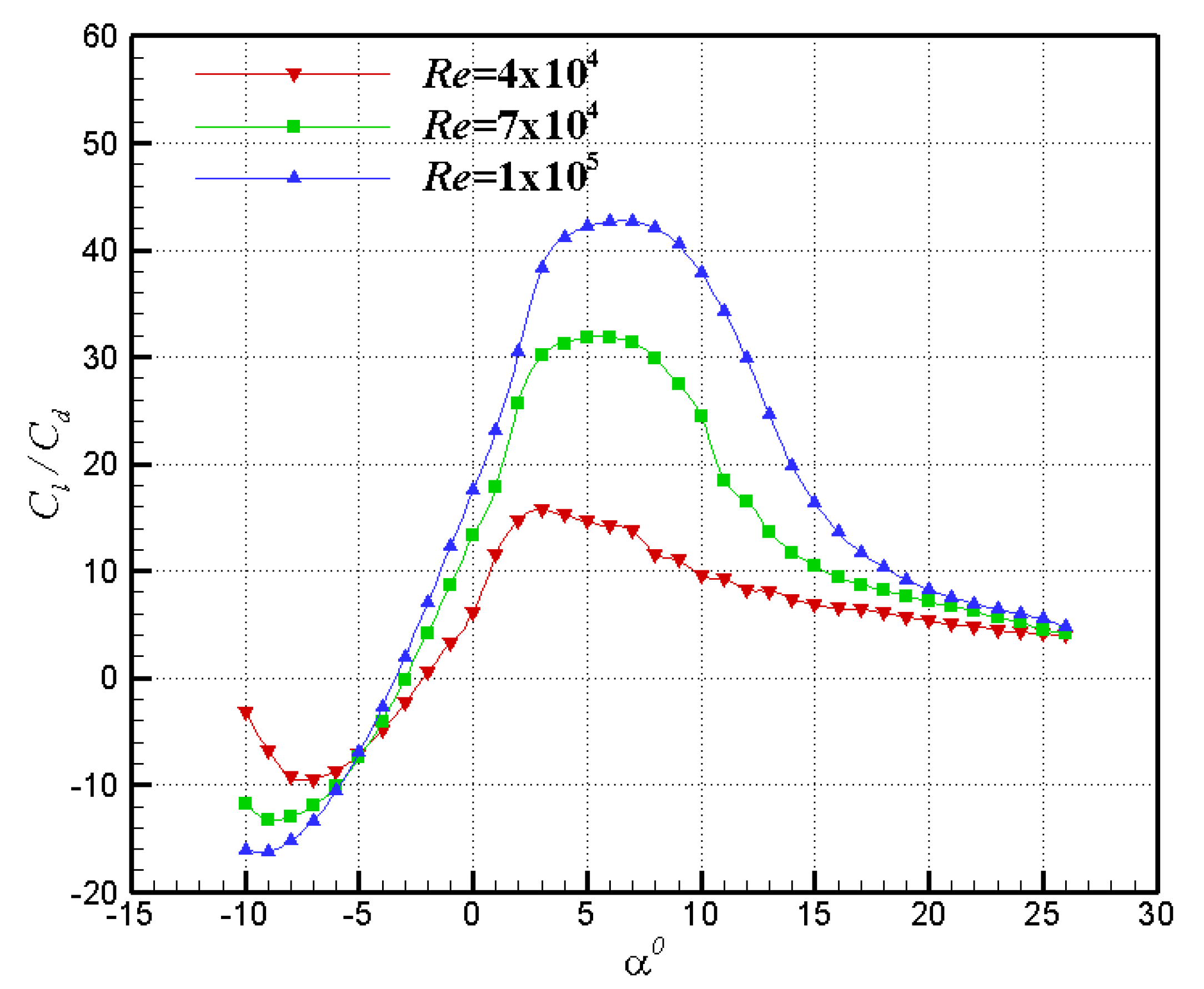
Figure 4 shows the results of a Reynolds number sensibility study made with XFoil over the performance of a NACA4418 airfoil at low Reynolds numbers when
Ncrit = 1. These data can be used to improve the BEM model, design an OPT blade, and predict the blade performance, points which will be developed in the next section. Furthermore, these data also provide the numerical simulation of 2D airfoil in accordance with the results of the lift and drag coefficients that will be shown in detail in
Section 4.
The definition of power coefficient (
Cp) for the blade can be written as:
where
Tm is the mechanical torque (N-m), which can be measured using a torque transducer during the wind tunnel experiment.
Figure 3.
The distributions of angle of attack in each section at V = 10 m/s and λ = 3, 5 and 7.
Figure 3.
The distributions of angle of attack in each section at V = 10 m/s and λ = 3, 5 and 7.
Figure 4.
Airfoil data calculated from XFoil with Ncrit = 1.0 for the BEM predictions.
Figure 4.
Airfoil data calculated from XFoil with Ncrit = 1.0 for the BEM predictions.
Improved BEM Method
An airfoil has stall phenomenon when flow separates at high angles of attack, typically greater than 15°. Beyond this angle, the lift of the airfoil drops and drag increases significantly. To overcome this stall problem in the blade design, Viterna and Corrigan [
16] have proposed a stall model which was successfully applied for predicting the lift and drag coefficients of a HAWT blade in the stall region. The rotational effect of the HAWT rotor blade is a typical case in which the so-called stall delay phenomenon occurs. This state is characterized by maintaining significant lift coefficient that is comparable with the 2D airfoil data measured in the wind tunnel with the occurrence of flow separation for the airfoil at a higher angle of attack beyond the stalled angle [
17]. Even though this phenomenon was first observed in propeller blades [
18], it has been applied to helicopters and we have even used our knowledge of this phenomenon (stall delay model) in wind turbine fields [
2,
6]. Because the pressure on the suction side of the blade is lower than on the pressure side, air tends to flow around the tip from the lower surface to the upper one and in this manner reduces both the lift together and the power production near the tip. This phenomenon is called tip-loss. In this study, the performance data of NACA4418 airfoil, calculated by XFoil at Reynolds number of 4 × 10
4, 7 × 10
4 and 1.0 × 10
5, were used in conjunction with the improved BEM model. The lift and drag coefficients were used to predict the blade performance with the angle of attack of less than 12°. When the angle of attack exceeds 12°, the VC stall model was performed to predict the performance of the blade in the stall region—the tip-loss factor and stall delay model were also combined with the improved BEM model to increase the accuracy of the performance prediction. All pertinent mathematical details can be found in [
2,
6].
3. Experimental Setup
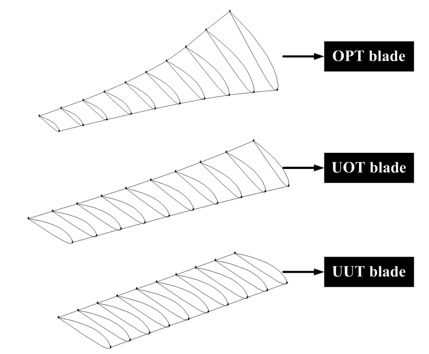
Three different HAWT blade models, shown in
Figure 5, have been tested inside the wind tunnel. The first one is the optimal (OPT) blade shape which was calculated by an in-house code developed using the improved BEM theory. It is composed of a NACA4418 airfoil that is tapered and twisted. Five parameters are needed to define a OPT blade shape design: (1) rated power; (2) rated wind speed; (3) design tip speed ratio; (4) number of blades; and (5) design angle of attack (
Table 1). In this paper, the design angle of attack has been set to 5.5° because it generates the maximum lift to drag ratio when using a Reynolds number of 1.0 × 10
5 (
Figure 4). All the design parameters are summarized in
Table 2. The second blade model is an untapered and optimal twist (UOT) blade that has a constant chord of 0.055 m. The twist distribution is the same as the OPT. The blade radius is also 0.36 m and the NACA4418 airfoil was also used. The final one is an untapered and untwisted (UUT) blade that has the same parameters as the UOT blade, except the twist distribution is set to 0°.
Figure 5.
Three test blade models for wind tunnel experiment.
Figure 5.
Three test blade models for wind tunnel experiment.
Table 1.
The blade design parameters of OPT blade.
Table 1.
The blade design parameters of OPT blade.
| Design parameters | Values |
|---|
| Rated power (W) | 50 |
| Rated wind speed (m/s) | 10 |
| Design tip speed ratio | 5 |
| Number of blades | 3 |
| Design angle of attack (°) | 5.5 |
| Airfoil type | NACA4418 |
Table 2.
Parameters of the OPT blade design.
Table 2.
Parameters of the OPT blade design.
| Seconds | r/R | Airfoil type | Chord length (m) | Twist angle, β(°) |
|---|
| 1 | 0.17 | NACA4418 | 0.096 | 25.92 |
| 2 | 0.26 | NACA4418 | 0.085 | 17.56 |
| 3 | 0.35 | NACA4418 | 0.072 | 12.20 |
| 4 | 0.44 | NACA4418 | 0.061 | 8.61 |
| 5 | 0.54 | NACA4418 | 0.053 | 6.08 |
| 6 | 0.63 | NACA4418 | 0.046 | 4.21 |
| 7 | 0.72 | NACA4418 | 0.041 | 2.78 |
| 8 | 0.81 | NACA4418 | 0.036 | 1.65 |
| 9 | 0.91 | NACA4418 | 0.033 | 0.75 |
| 10 | 1.00 | NACA4418 | 0.030 | 0.00 |
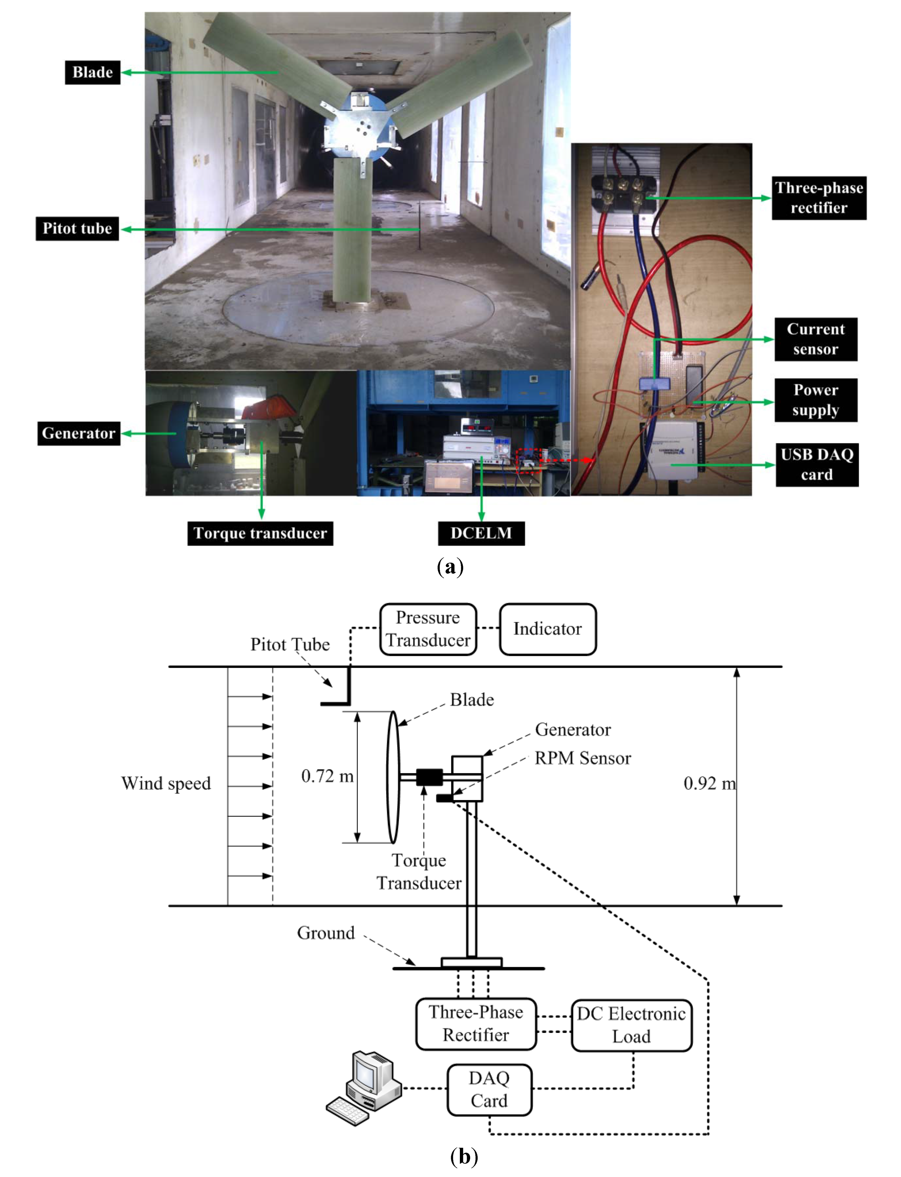
Figure 6 shows the results for the blades when tested inside the wind tunnel. The full scale wind tunnel experiment was used to provide the data for comparison with the BEM code. The test section of this wind tunnel is 1,440 mm long and the area of cross section is 1200 mm wide × 920 mm high. The specifications of the wind tunnel itself, which offers a maximum wind speed of 30 m/s, has been verified through many parameters including: structure vibration, temperature, stability, flow uniformity, turbulence intensity, flow angularity, and boundary layer thickness. The mean flow uniformity is about 0.37%, the turbulent intensity is less than 0.35% and the boundary layer thickness is about 60 mm at the inlet cross section. The flow angularity of pitch and yaw angles are, respectively, about ±0.415° and ±0.97° at a wind speed of 20 m/s. A pitot-static tube was adopted to measure the free stream velocity in the test section because it is stable, accurate and convenient to calibrate. A variable reluctance pressure transducer was connected to the pitot-static tube and transfers the pressure difference between the total pressure and the static pressure into electric voltage. The small analog signal was then amplified and converted using an analog/digital converter to digital dataflow and saved onto a personal computer (PC). The pressure transducer was calibrated using a micro manometer and certified. The flow speed in the test section was then calculated using the incompressible steady Bernoulli’s equation [
19].
Figure 6.
(a) The tested models setup inside the test section of full-scale wind tunnel; (b) The schematic of the tested models setup inside the test section of the full-scale wind tunnel.
Figure 6.
(a) The tested models setup inside the test section of full-scale wind tunnel; (b) The schematic of the tested models setup inside the test section of the full-scale wind tunnel.
In the wind tunnel experiments, the area ratio is defined as A
b/A
w, where A
b is the blade swept area and A
w is the cross section area of the wind tunnel test section. This area ratio is an index of the wind tunnel experiment for the HAWT system and allows us to have a maximum ratio of 30% without any interference effects from the wind tunnel wall on the power coefficient measurement, according to the reference [
20]. In comparison with the area ratio of 8.8% for the NREL full-scale wind tunnel experiments performed using a blade with a radius of 5 m [
21], in this study, the area ratio of the models is 36% and these models were tested in a closed test section. Obviously, our models are a little larger than the allowed maximum ratio, hence the blockage effect in the present study will also be a little higher. After our careful calculation and analysis, following the model of Barlow
et al. [
22], the blockage effect would be expected to cause a wind speed of 10 m/s, as an example, to be reduced by about 3% in the wind tunnel test. Therefore, the results of the power coefficient measurements with respect to the effective wind speed will also show an uncertainty (error) of 3% or less, which is still satisfactory in the experiments. Furthermore, the Betz limit also indicates that as the rotor blade transports, the efficiency from wind energy (power coefficient) should have a maximum value of 59%. Our test results, shown in following section, do not exceed the Betz limit.
In
Figure 6 we can see the torque transducer used to measure the mechanical torque; it was mounted on the main shaft between the rotor blade and the generator. This measurement method, using a torque transducer for a HAWT blade, has been used by many authors [
10,
23], including as Kang
et al. [
23] who showed that the torque transducer can successfully measure the mechanical torque for power coefficient calculation. For the most accurate results, it is essential that the torque transducer be mounted as close as possible to the rotor blade to decrease any shaft frictional losses that might interfere with the measurement of the power coefficient.
The function of a high current DC electronic load module (DCELM) is to simulate the different loads of the circuit. If the circuit loads is changed by the DCELM, the rotational speed of the blade will also be changed. The operating region of the DCELM has four major functions: (1) constant current; (2) constant resistance; (3) constant voltage; and (4) constant power (between 0–60 V and 0–120 A). To be thorough, the signal of the rotational speed for the blade also needs to be measures. In this study a tachometer and proximity switch were used to measure the blades RPM. In this case, only the DC signal can be analyzed, so we used the simplest type of rectifier is a diode bridge circuit which converts the AC to fluctuating DC. The acceptable input voltage of Analog/Digital converter is below 10 V. In order to measure higher voltages, the amount should be shrunk to one quarter. The current meter is an onboard function of the DC electronic load which directly converts the DC current into DC voltage and obtains the signal using an AD converter.
The data acquisition for voltage outputs from these sensors were performed by National Instrument (NI) USB-6008 12 bit AD converter. For the measurement of voltage, current and rotational speed in wind tunnel, the sampling frequency was fixed at 3 kHz and sampled at 6 k per point. The measuring time of data acquisition is 2 s. NI LabVIEW software was used to construct the data acquisition program.
5. Results and Discussion
All the wind tunnel experiments were perfromed at constant wind speed of 10 m/s. The different tip speed ratios (λ) were obtained by adjusting the wind turbine’s rotational speed. The mechanical torque, which is used to compute the power coefficient (
Cp), was measured by averaging ten values of the torque transducer.
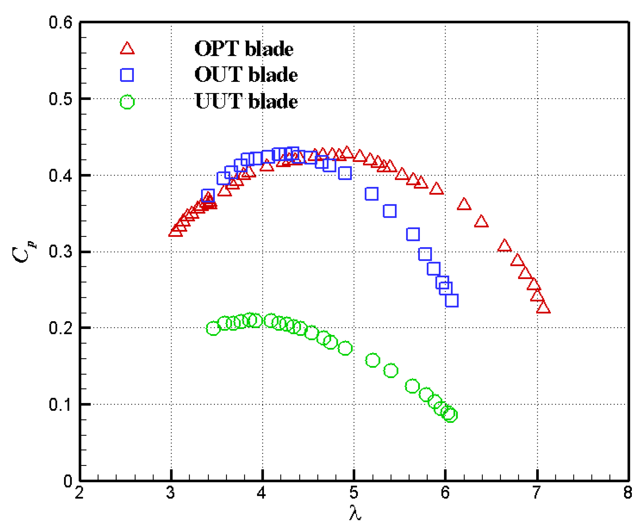
Figure 10 shows the power coefficient distributions of the OPT, OUT and UUT blades at different tip speed ratios.
Figure 10.
The experimental results of power coefficient as function of tip speed ratio for OPT, UOT and UUT blades at V = 10 m/s.
Figure 10.
The experimental results of power coefficient as function of tip speed ratio for OPT, UOT and UUT blades at V = 10 m/s.
The OPT blade has a maximum power coefficient of
Cp = 0.428 at λ = 4.92, which is very close to the design tip speed ratio, which is 5. It can be proven that the OPT blade conforms to the results of the BEM design. Unexpectedly, the UOT blade also obtained a maximum
Cp value of 0.428, while the tip speed ratio is 4.32. Although both the OPT and the OUT blades obtain an excellent power coefficient, we conclude that the OPT blade is better than the UOT blade because it has a higher range of high power coefficients. Indeed, even if the two blades have a similar power coefficient from a tip speed ratio of 3 to 5, the performances of the OUT blade quickly decreases after passing λ = 5 while the OPT blade keeps its high power coefficient until λ = 6. It can be understood from
Figure 10 that the OPT blade operates quite well at high rotational speed. On the other hand, the UUT blade obtains its maximum power coefficient
Cp = 0.210 at λ = 3.86, which is lower than for both the other blades. The main reason why
Cp is so low is due to the stall phenomenon, which will be examined in more detail later.
The first calculations of power coefficient were undertaken using the in-house code which was developed using the BEM theory. All the settings used were set to correspond to the different cases discussed in this paper. The airfoil data, function of the Reynolds number (
Re) given by XFoil have been combined into the code. We developed to compute the power coefficient of tip speed ratios from 0 to 9. This means that the operational range of the NACA4418 used would be from angle of attack −5 to 55, but from
Figure 4 it can be clearly seen that we only have the data for angles of attack from −10 to 28. Here the Viterna-Corrigan stall model [
13] was combined with our code to successfully predict the blade performance both near the stall region and after the stall point.
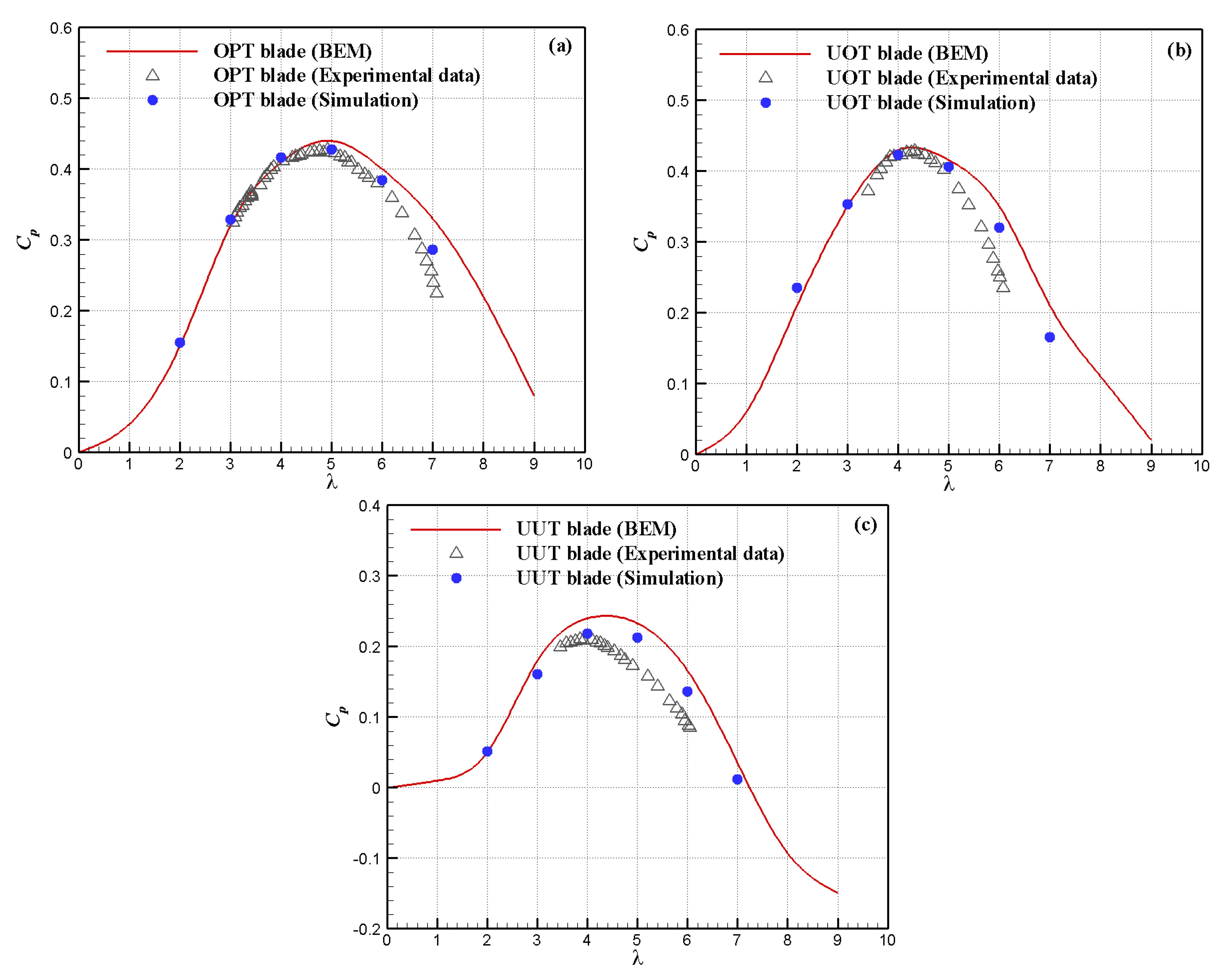
Figure 11 show the power coefficient comparison as a function of the tip speed ratio for the OPT, the UOT and the UUT blades. However the predictions made using the improved BEM method and CFD simulation have a good trend of power coefficient curves when compared with the experimental data.
The BEM method uses some correction factors such as tip loss and rotational augmentation, and these have been included in our in-house code. When the turbine blade was operated at a tip speed ratio of less than 3, the distributions of angle of attack was always greater than 20° and the significant stall effects are occurred at whole blade section for these three blades. This solution is quite good for predicting Cp for low tip speed ratios. Also, we determined that the Viterna-Corrigan stall model is available for this BEM code. Though the BEM method predicts a good trend for higher tip speed ratios (λ > 5), the Cp values clearly over-predict after λ = 5 for these blades. The small differences between the BEM and CFD predict Cp at high tip speed ratios (λ > 5) probably come from the difference in boundary layer development and particularly related to whether or not the flow is turbulent from the leading edge. Indeed, this phenomenon of boundary layer development is not mathematically compatible with the BEM code. However, this could be an indication that the 2D airfoil data used from XFoil are available for a high angle of attack.
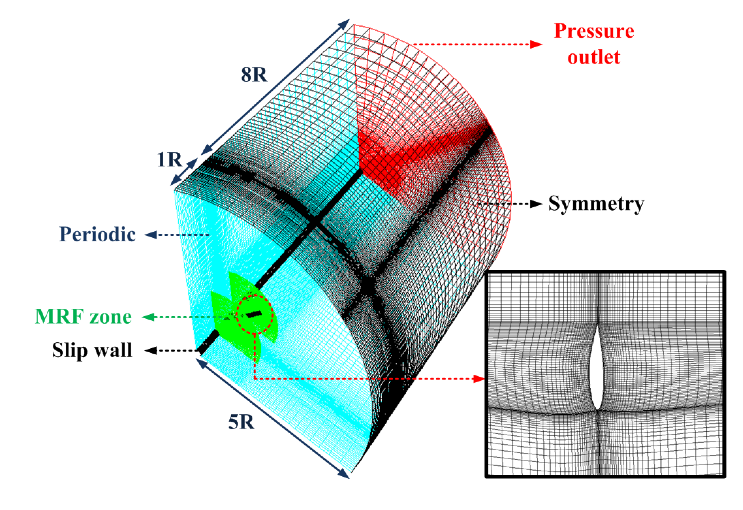
The CFD simulation method gives similar results to the experimental data for all three blade models, and is particularly good at identifying the maximum point of
Cp, which comes out the same for all three. This conclusion strongly supports the fact that we can use the CFD simulation to further numerically observe the pressure distribution and the flow fields along the spanwise direction of the blade.
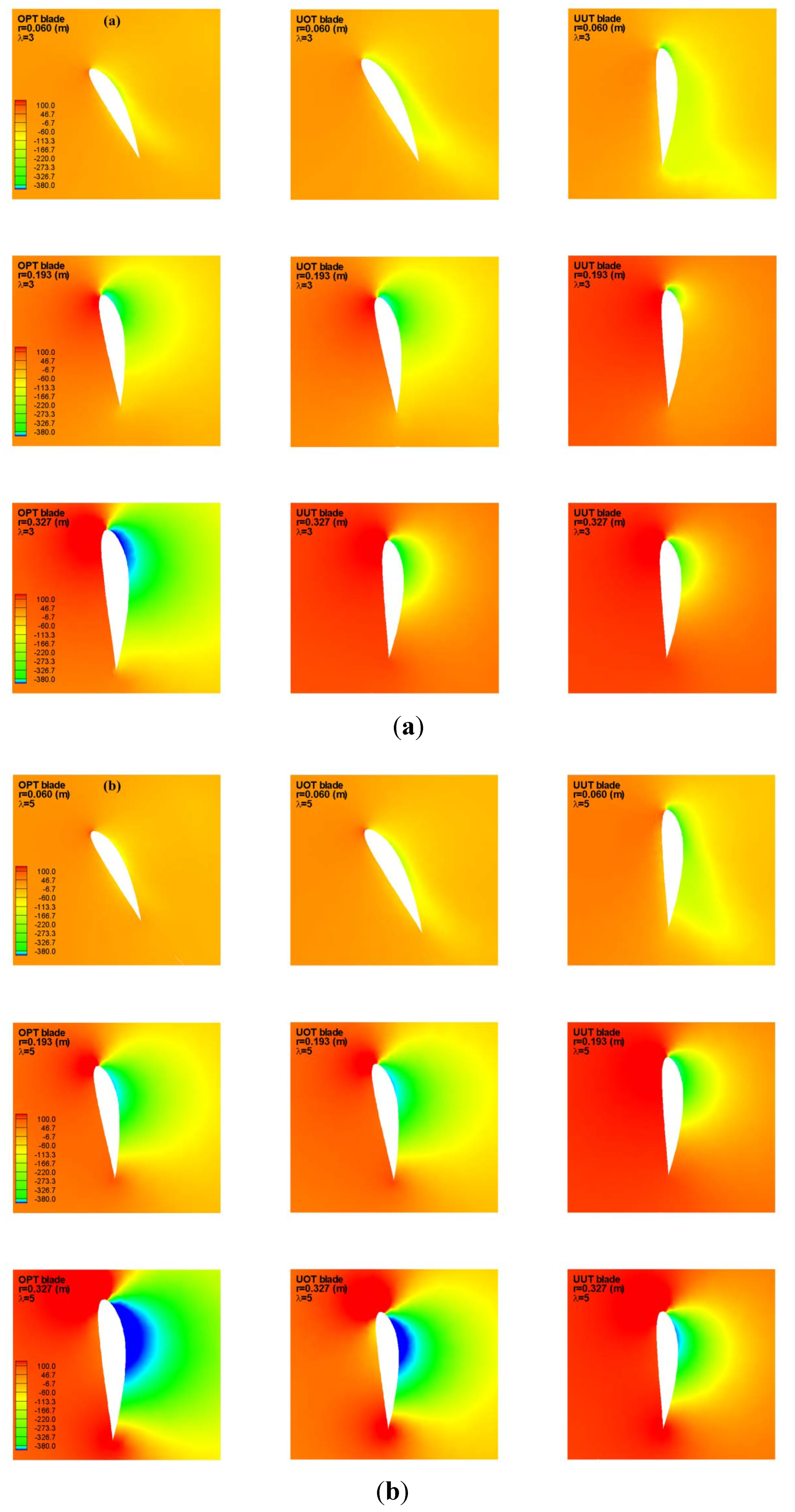
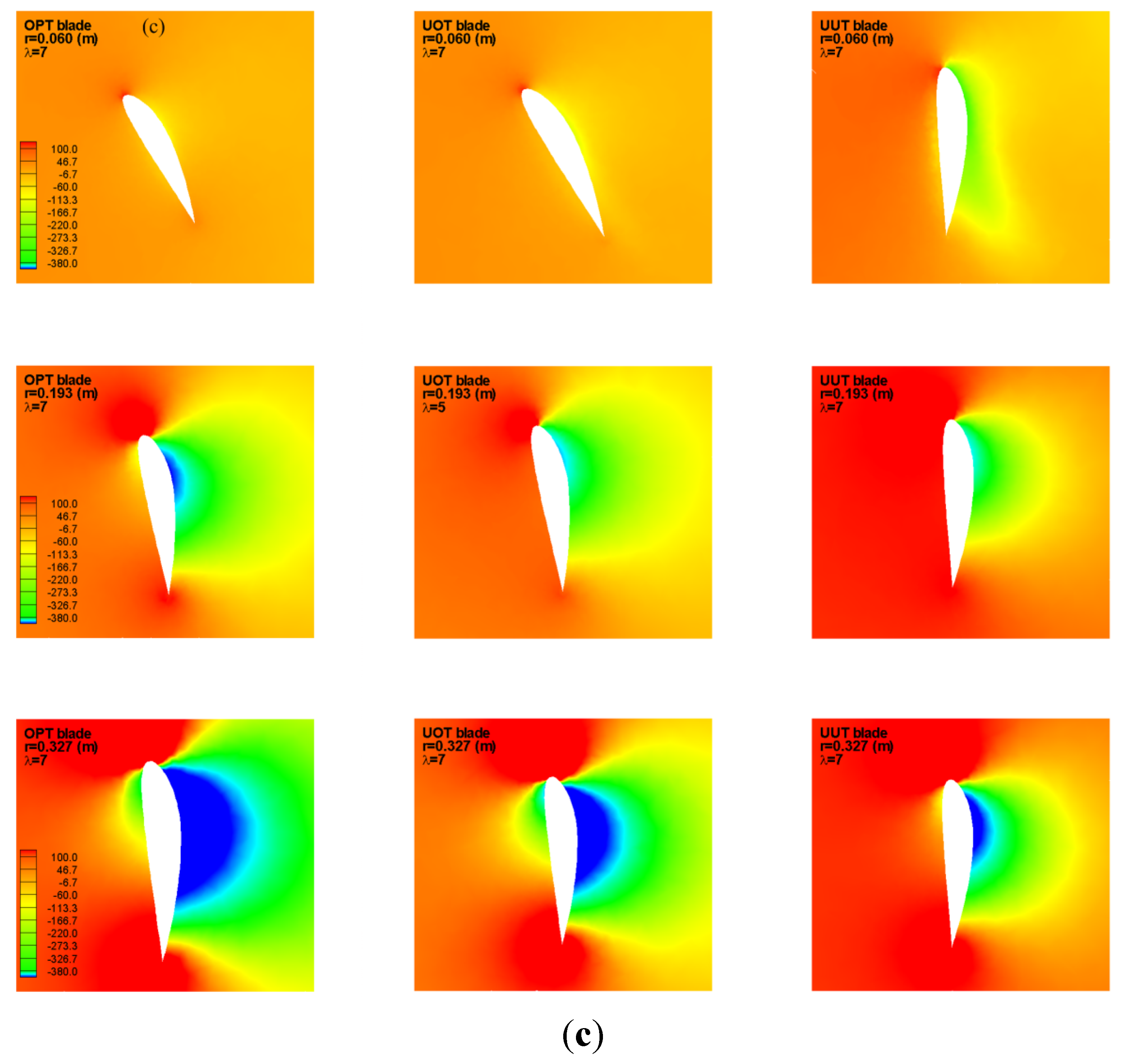
Figure 12 shows the sectional pressure fields of different radial sections for the OPT, the UOT and the UUT blades. Several things should be noticed. First of all, it can be seen that there is almost no pressure difference at the blade roots (
r = 0.060 m) for λ = 3, 5, and 7. Similarly, we find that the OPT and the UOT blades have almost the same pressure difference at
r = 0.193 m for λ = 3 and λ = 5 while the UUT blade has a larger pressure difference. The larger difference of the pressure for these three blades is at around the two-thirds mark (
r = 0.327 m). Also, in comparing the upper and lower surfaces at λ = 7 for these blades, we see that the OPT blade has a slightly larger low-pressure area than other two, which may be why more power is predicted for the OPT blade, a result which explains why the OPT blade produces more
Cp value than other two blades in the experimental results. From the experimental data (
Figure 10), the
Cp value of the OPT blade is slightly larger than the UOT blade and a fair amount larger than the UUT blade at λ = 5, which is the design tip speed ratio. The differences in the OPT and UOT blades can be observed in the CFD simulation shown as
Figure 12b, in which the pressure distribution is almost the same at
r = 0.060 m and
r = 0.193 m and there is a slight difference at
r = 0.327 m.
Figure 11.
(a) Power coefficient calculated for OPT blade using BEM and simulation methods as compared with experimental data; (b) Power coefficient calculated for UOT blade using BEM and simulation methods as compared with experimental data; (c) Power coefficient calculated for UUT blade using BEM and simulation methods as compared with experimental data.
Figure 12.
(a) The distributions of the pressure field for OPT, UOT and UUT blades in r = 0.060 (m), r = 0.193 (m) and r = 0.327 (m) at V = 10 (m/s) and λ = 3; (b) λ = 5; (c) and λ = 7.
Figure 12.
(a) The distributions of the pressure field for OPT, UOT and UUT blades in r = 0.060 (m), r = 0.193 (m) and r = 0.327 (m) at V = 10 (m/s) and λ = 3; (b) λ = 5; (c) and λ = 7.
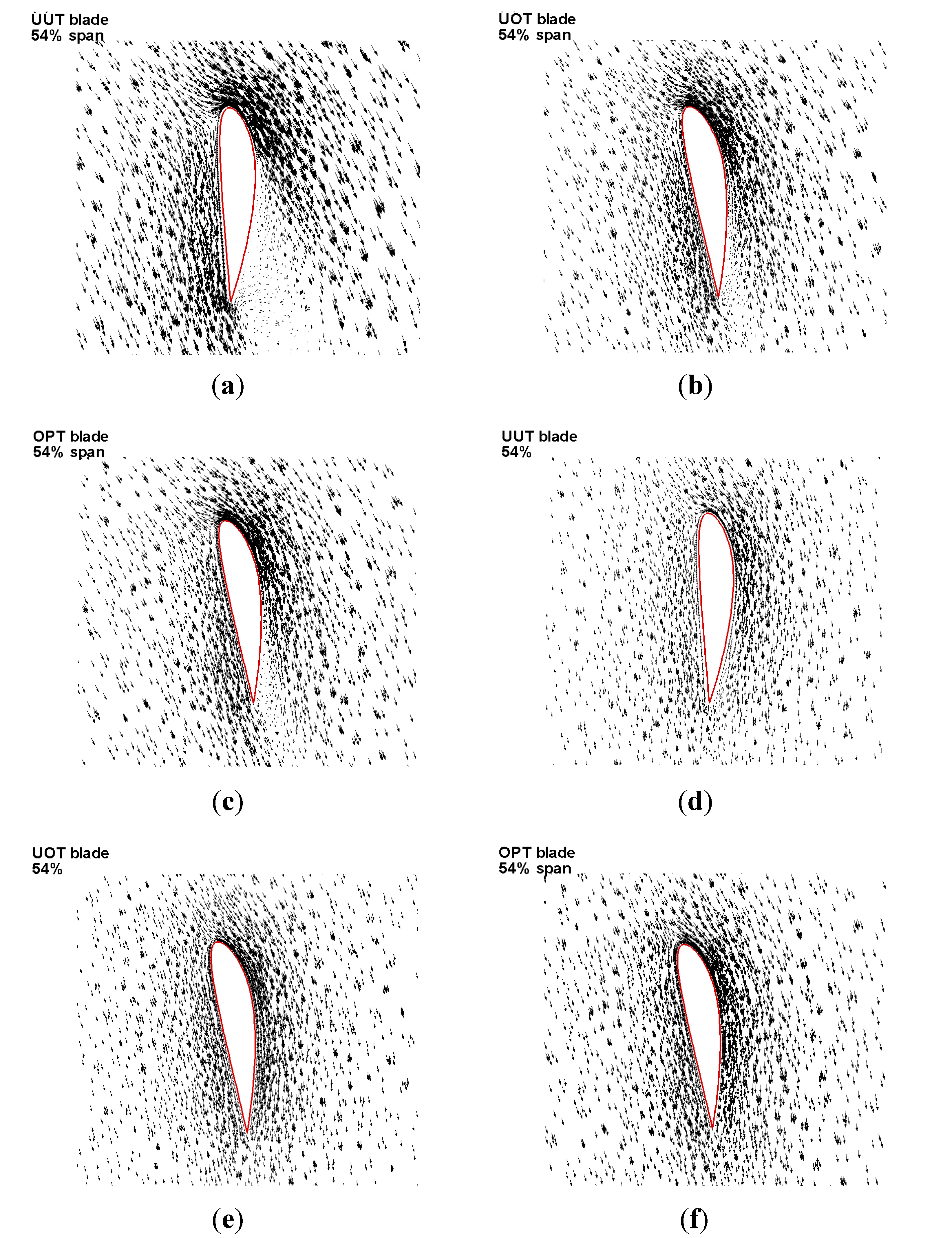
Figure 13a–c shows the vector plots at 54% of the span of the OPT, the UOT and the UUT blades at λ = 3 and
V = 10 m/s. It is clear that the UUT blade suffers from a deep stall phenomenon over the entire suction surface, mainly because the operating angle of attack is about 21°. This phenomenon partially explains why the power coefficient of the UUT blade is lower than the OPT and the UOT blades. As expected, the vector plots for the OPT and the UOT blades at λ = 5, which is the design tip speed ratio, show that the flow behaves well as shown in
Figure 13e,f. It should be noted that though the flow is good at λ = 7 for these three blades, the maximum lift to drag (
Cl/
Cd) ratio of λ = 5 is 42, which is larger than λ = 7 (
Cl/
Cd = 23). Consequently, the OPT blade obtains its best power coefficient (0.428 from the experimental data) at λ = 5.
The rotational effect of the HAWT rotor blade can lead to the so-called stall delay phenomenon, which is characterized by maintaining a significant lift coefficient. This situation is like the corresponding two-dimensional (2D) airfoil data measured in a wind tunnel in which the flow separation for the airfoil is at a higher angle of attack, beyond the stalled angle. Although the angle of attack is greater than 12° in 54% span at λ = 5 for the UUT blade,
Figure 13d implies that the flow is still appropriate and the lift coefficient is 1.933.
Figure 13e,f also show that the UOT and OPT blades have a healthy flow with an angle of attack of 5° in 54% span at λ = 5. The lift coefficients for these are 1.922 for the UOT blade and 1.936 for the OPT blade. These results were calculated using a Fluent
k-
ω SST turbulence model.
Figure 13.
(a) The vector plots of flow field for UUT blade in 54% at V = 10 (m/s) and λ = 3; (b) The vector plots of flow field for UOT blade in 54% at V = 10 (m/s) and λ = 3; (c) The vector plots of flow field for OPT blade in 54% at V = 10 (m/s) and λ = 3; (d) The vector plots of flow field for UUT blade in 54% at V = 10 (m/s) and λ = 5; (e) The vector plots of the flow field for the UOT blade in 54% at V = 10 (m/s) and λ = 5; (f) The vector plots of flow field for OPT blade in 54% at V = 10 (m/s) and λ = 5.
6. Conclusions
The wind tunnel test results presented in this paper show that the OPT and the UOT blades obtain the same maximum power coefficient (Cp = 0.428) but at different tip speed ratio points. However, we conclude that the OPT blade is better than the UOT blade because its measured power coefficient is higher over a wider range of tip speed ratios, which go from 4.5 to 7. The UUT blade obtains the lowest Cp value because it almost always operates in stall conditions, indicating that the optimal design for the blade shape using the BEM method is needed, especially in the distribution of twist and chord length along the direction of the blade, spanwise. This paper also shows that the in-house code, which uses the BEM theory, is useful not only for designing the optimal blade shape but also at predicting the blade performance.
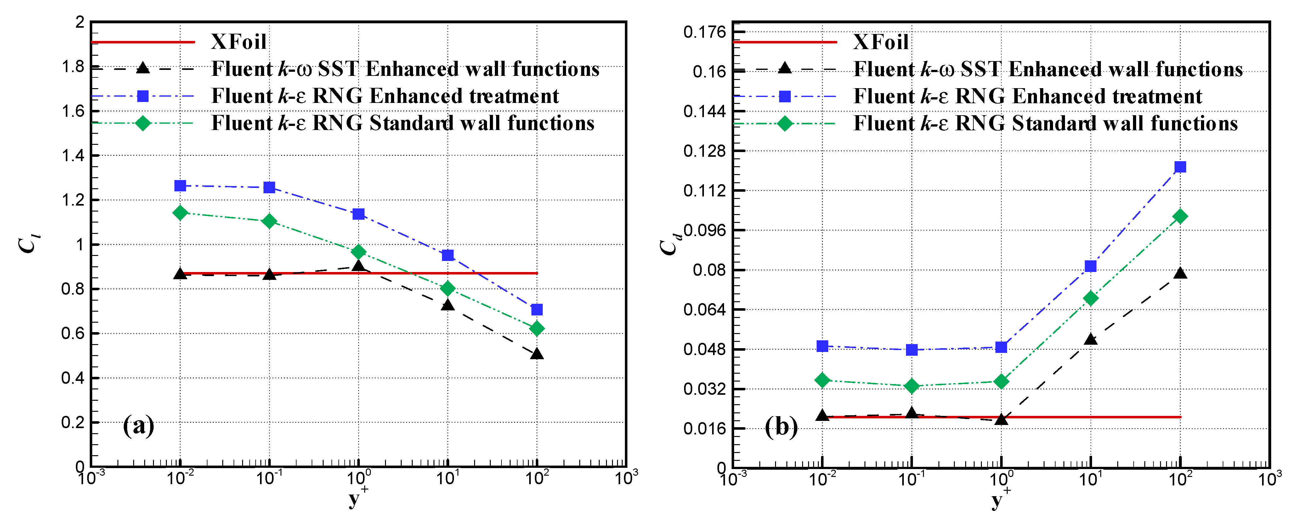
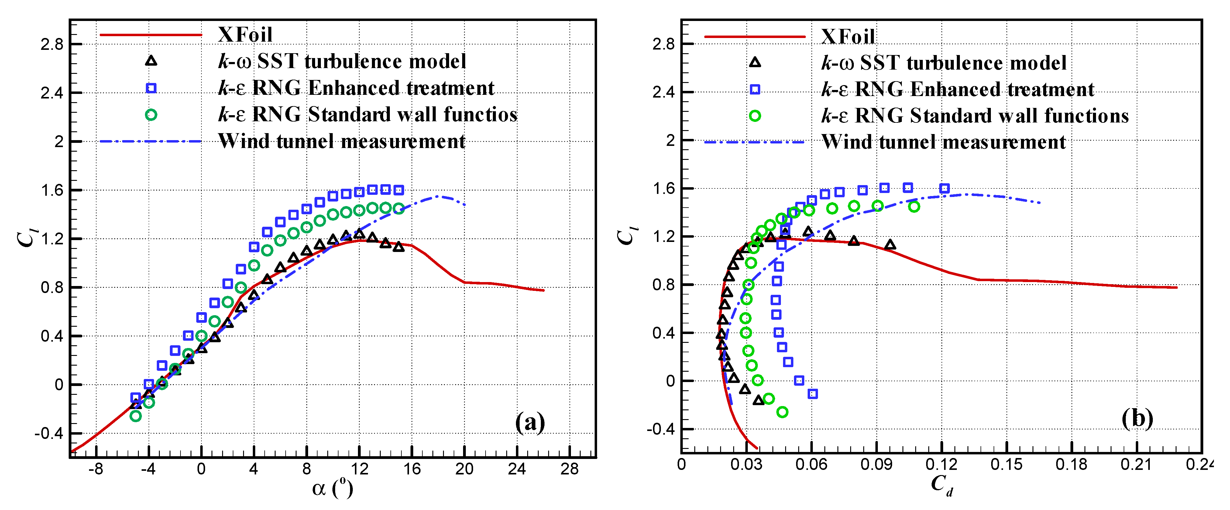
This review has also shown that XFoil is a good tool for predicting the lift coefficient, although in our test it tended to underestimate the drag coefficient a bit. This is shown in the CFD simulations using the commercial code Fluent, which consistently computed the same lift coefficients but higher drag coefficients.
Detailed flow fields were also investigated using full 3D CFD simulations by means of the commercial code Fluent and the k-ω SST turbulence model. The good agreement between the power coefficient computed by the Fluent package and the experimental data has been used in the validation process where it indicates that the Fluent package can be used to successfully predict the performances of a wind turbine.


