Second-Order Discrete-Time Sliding Mode Observer for State of Charge Determination Based on a Dynamic Resistance Li-Ion Battery Model

Abstract
:1. Introduction
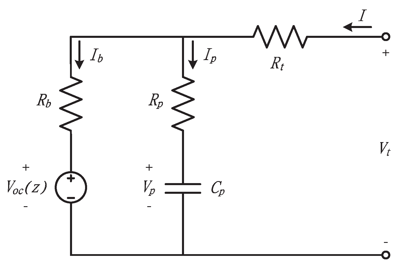
2. Battery Modeling
3. Second-Order DSMO for SOC Estimation
4. Experimental Results
- improvement of the battery modeling accuracy with the dynamic resistance varied with the operating conditions;
- the SOC estimation method using the second-order DSMO for the elimination of chattering.
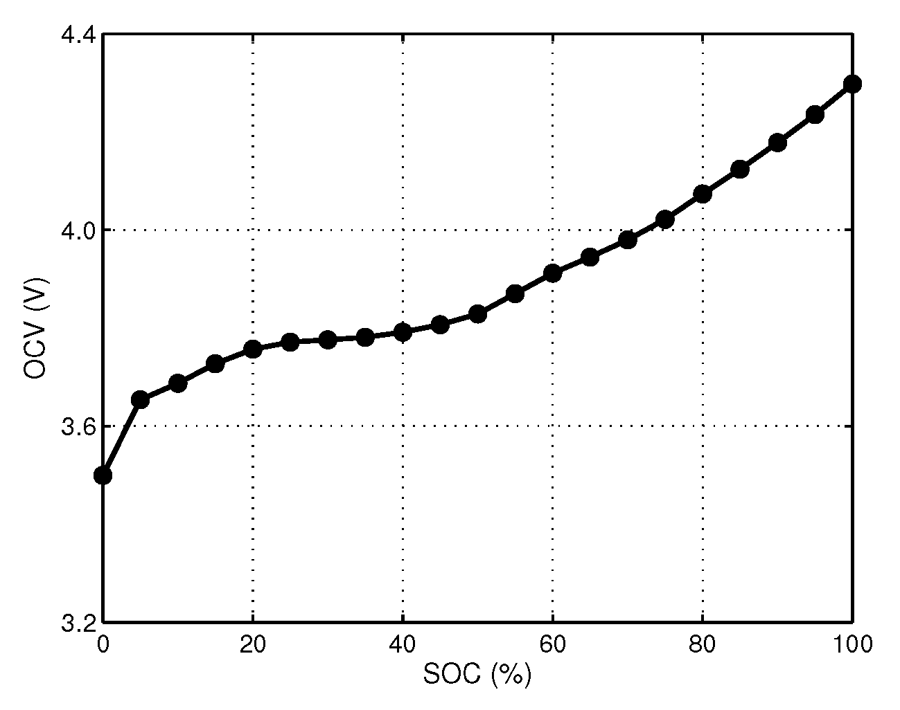
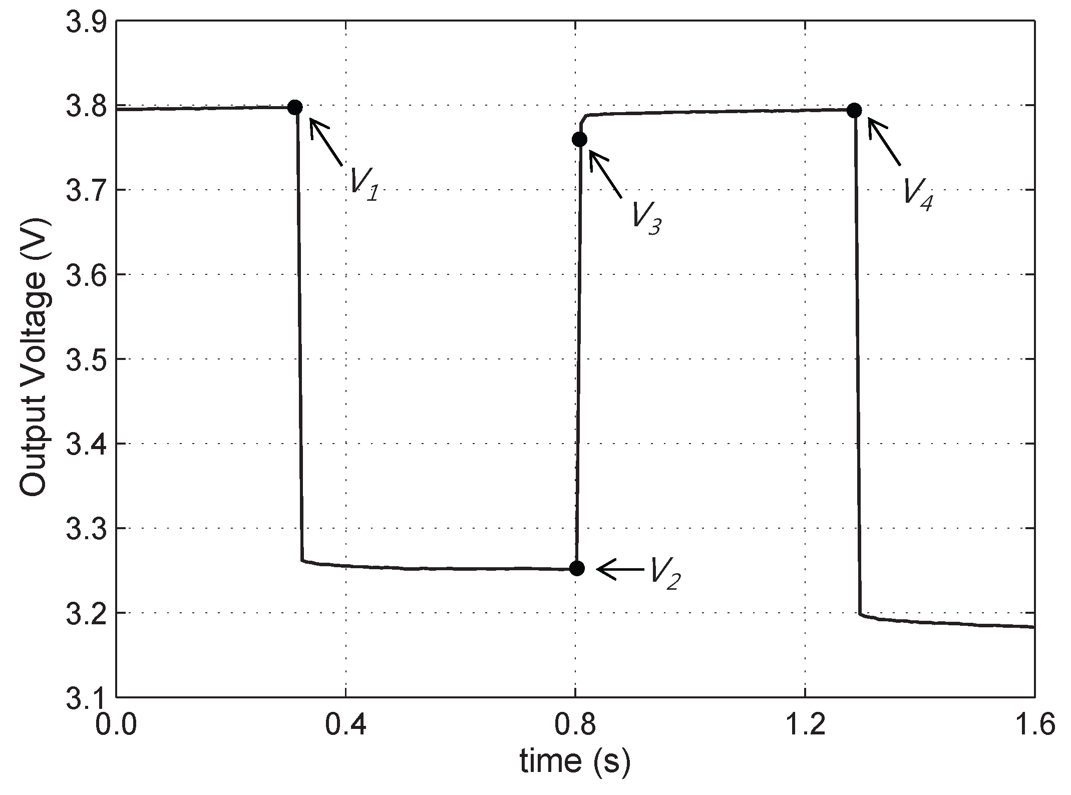
4.1. Parameter Extraction
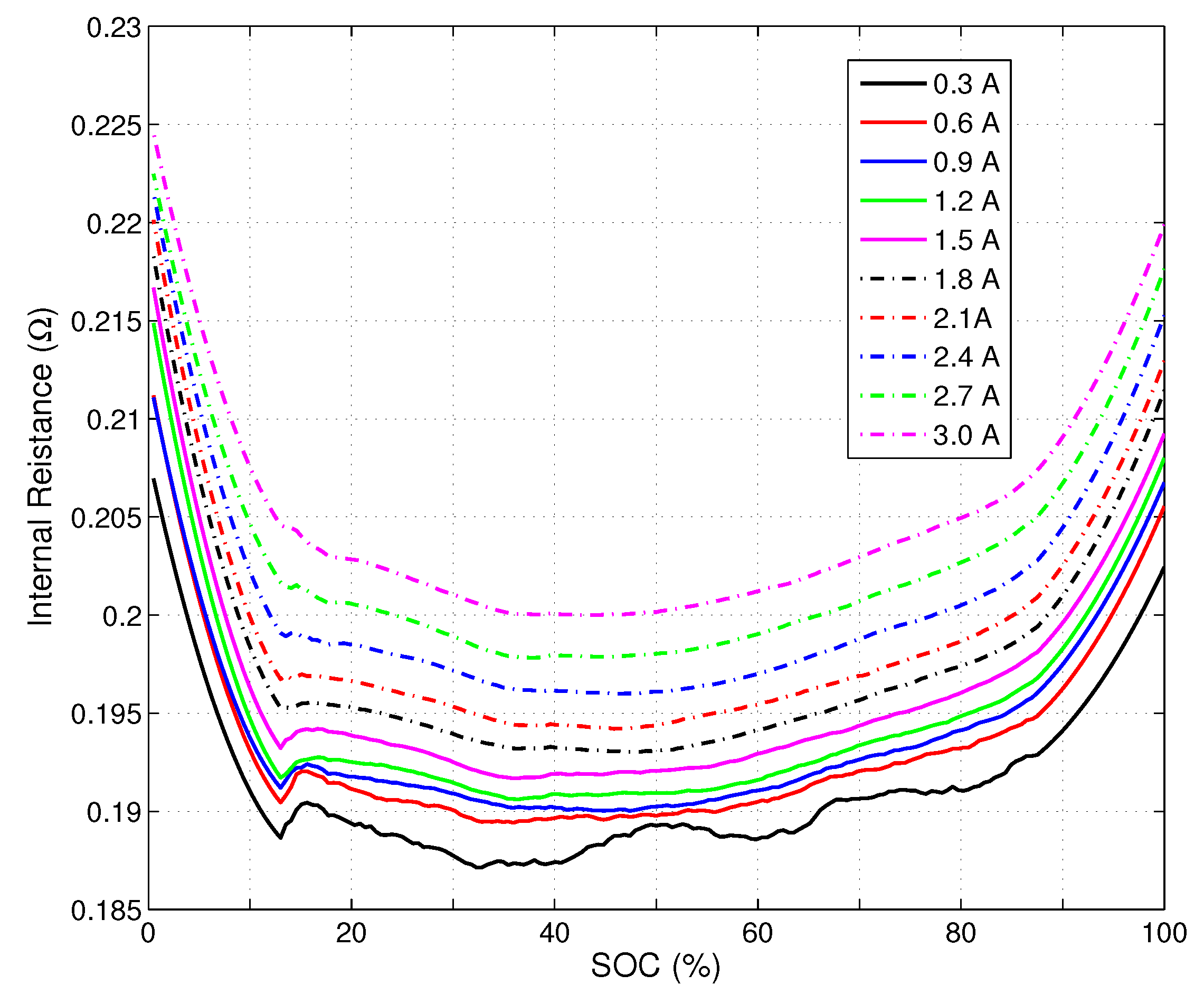
4.2. Dynamic Resistance

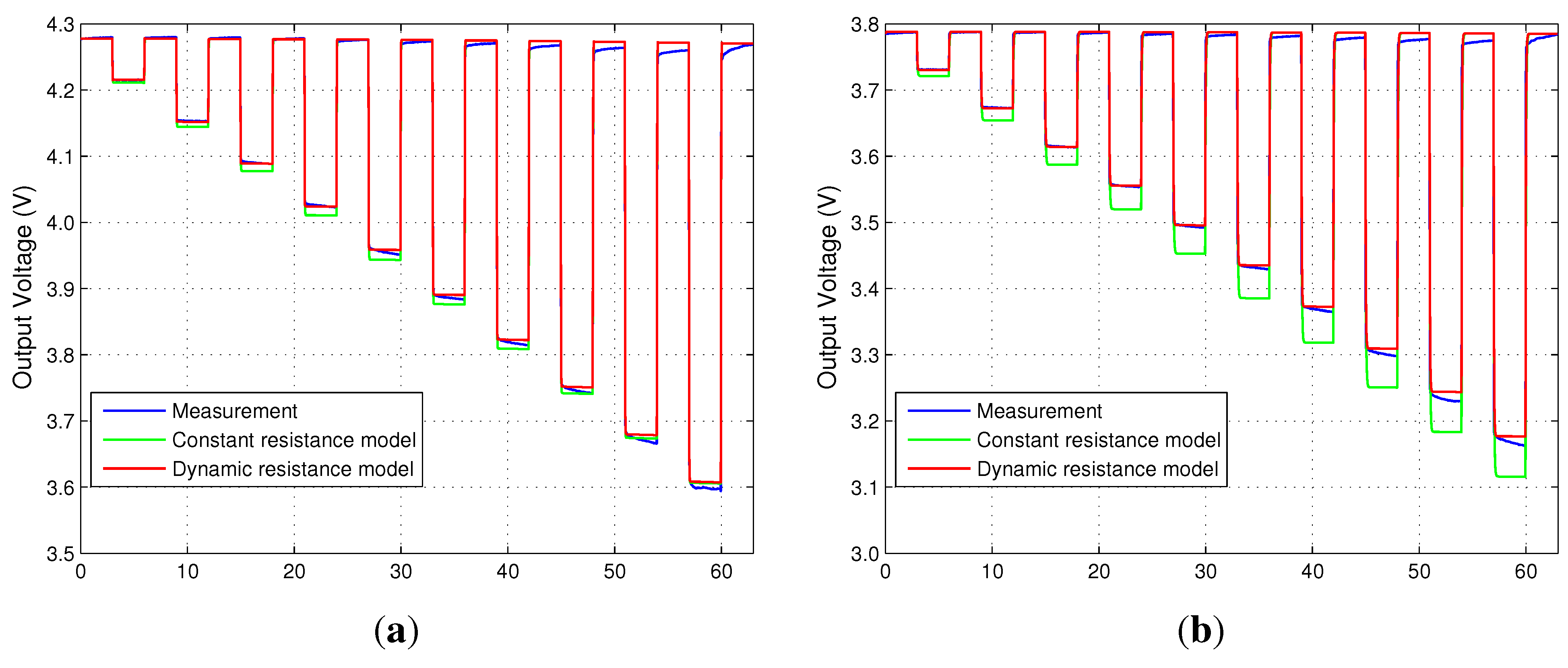
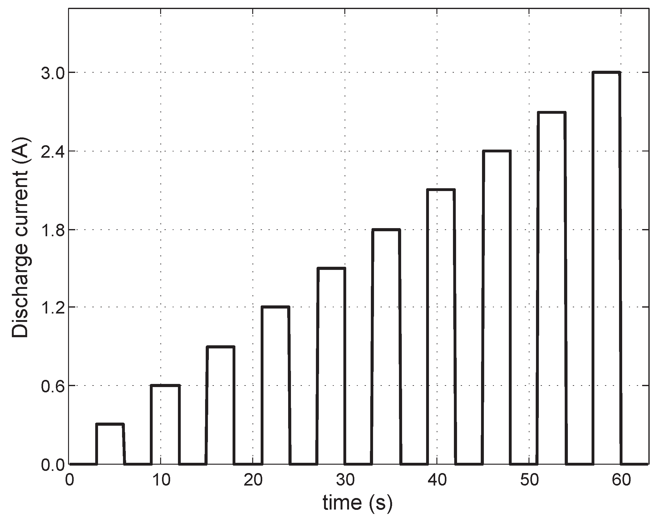
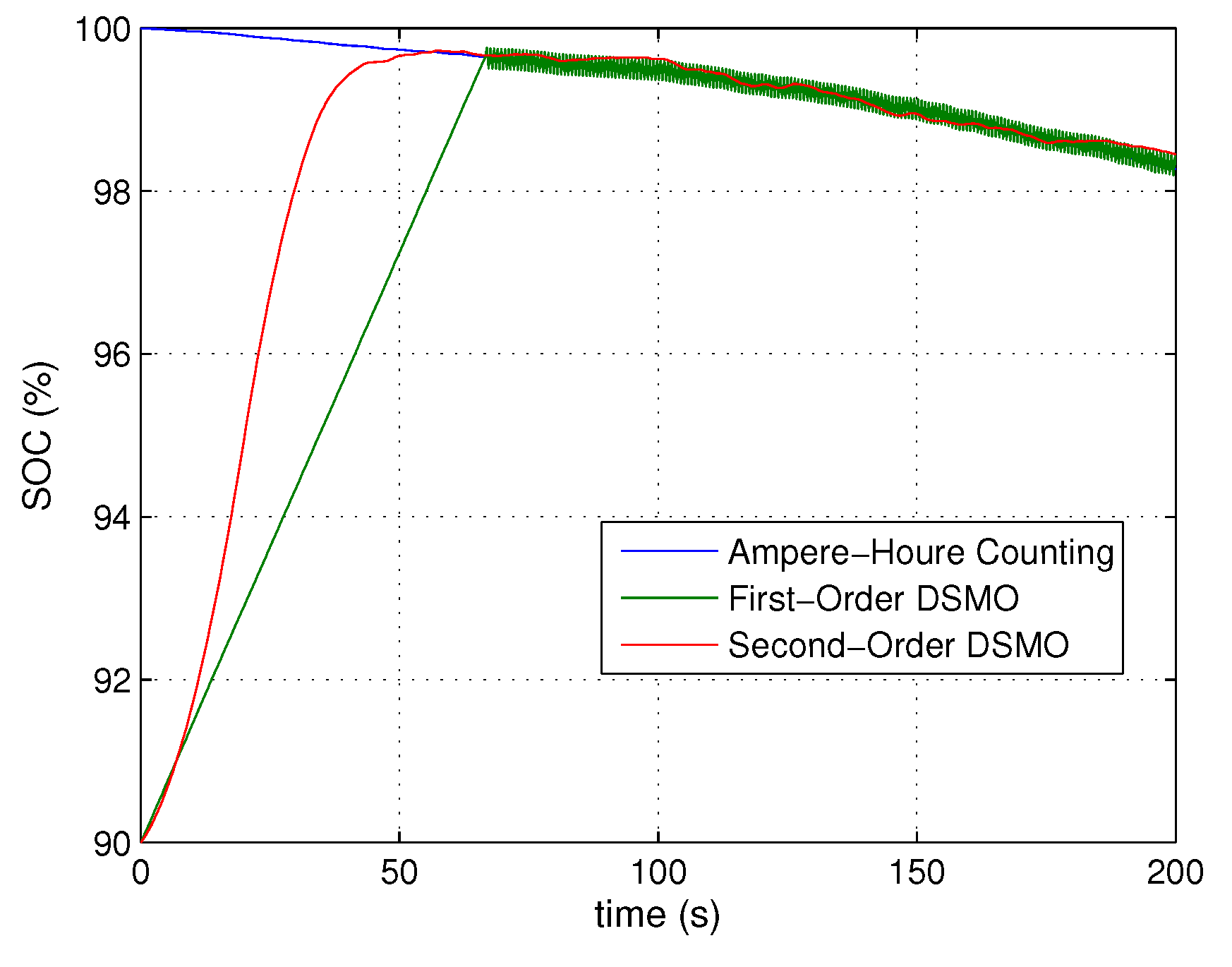
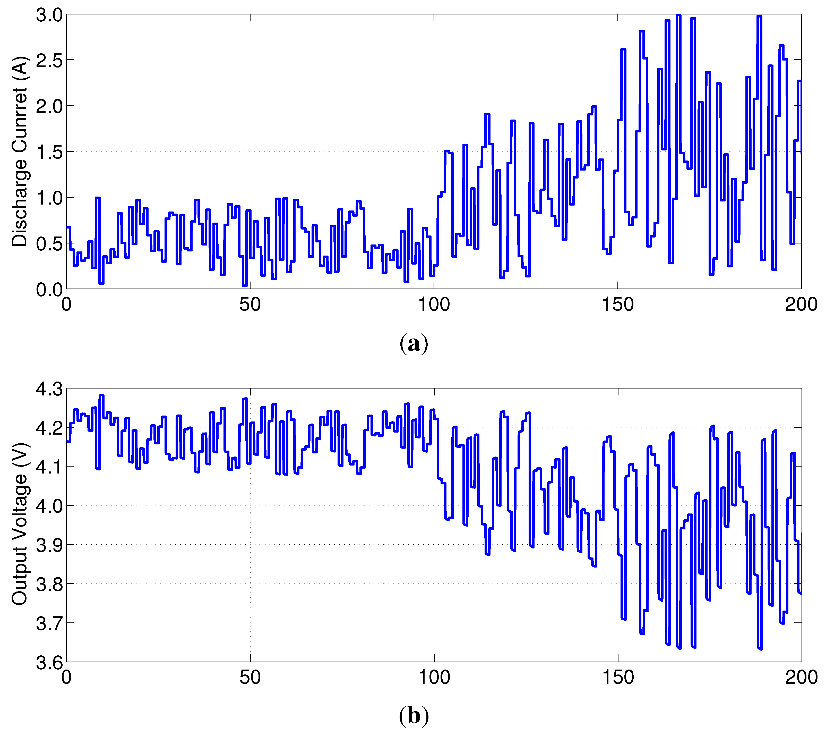
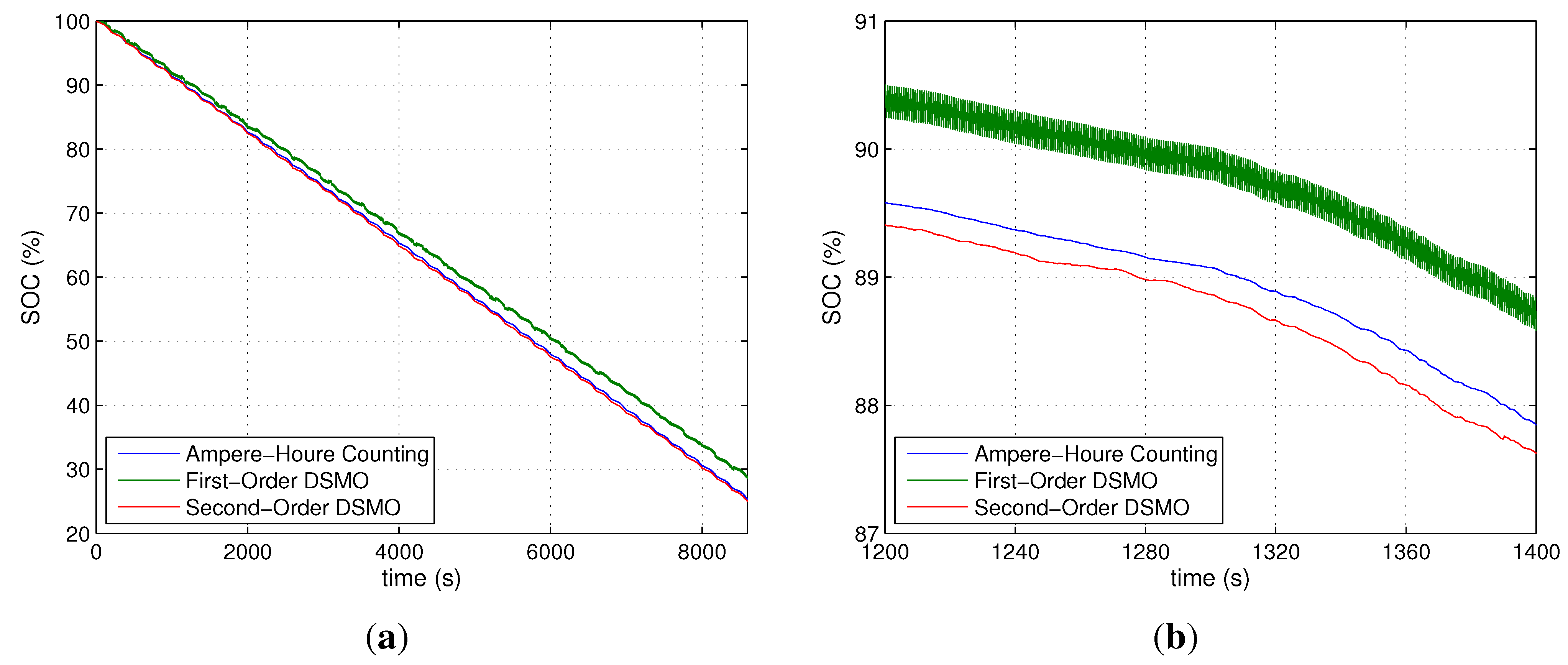
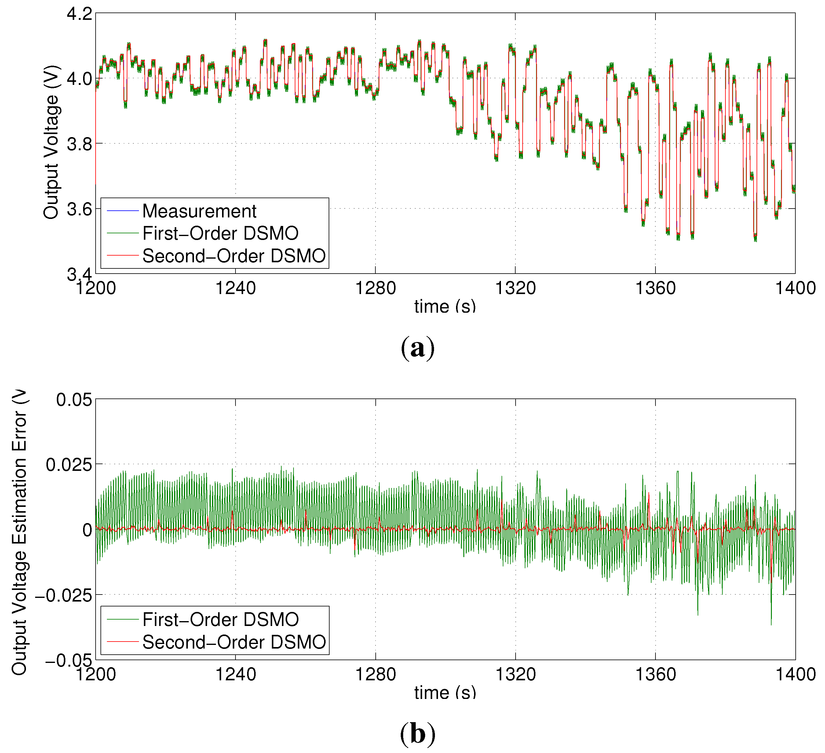
4.3. Random Current Discharge Test

5. Conclusions
Appendix: Stability Analysis
- Case 1 : suppose that .In this case, we have:By Lemma 1 in [13], for , there exists a bounded function F(k) ≥ 0 such that:where:Thus, Equation (18) can be written as follows:From Equation (22), we obtain the state equations:where:It is easily to ensure the convergence of Z(k) when eigenvalues’ modules of matrix A are smaller than one. Therefore, the convergence of the estimation error is also guaranteed.
- Case 2: .In this case, Equation (18) can be expressed as:Then we have:where:Consequently, if the uncertainty Λ(k) satisfies the condition in Equation (8) and eigenvalues’ modules of matrix A’ are smaller than one, Z(k)′ is bound. Also, the estimation error is bounded.
Acknowledgments
Conflicts of Interest
References
- Xing, Y.; Ma, E.W.; Tsui, K.L.; Pecht, M. Battery management systems in electric and hybrid vehicles. Energies 2011, 4, 1840–1857. [Google Scholar]
- Piao, C.; Fu, W.; Lei, G.; Cho, C. Online parameter estimation of the Ni-MH batteries based on statistical methods. Energies 2010, 3, 206–215. [Google Scholar] [CrossRef]
- Hu, X.; Sun, F.; Zou, Y. Estimation of state of charge of a lithium-ion battery pack for electric vehicles using an adaptive Luenberger observer. Energies 2010, 3, 1586–1603. [Google Scholar] [CrossRef]
- Chen, M.; Rincon-Mora, G.A. Accurate electrical battery model capable of predicting runtime and IV performance. IEEE Trans. Energy Convers. 2006, 21, 504–511. [Google Scholar] [CrossRef]
- Piller, S.; Perrin, M.; Jossen, A. Methods for state-of-charge determination and their applications. J. Power Sources 2001, 96, 113–120. [Google Scholar] [CrossRef]
- Alzieu, J.; Smimite, H.; Glaize, C. Improvement of intelligent battery controller: State-of-charge indicator and associated functions. J. Power Sources 1997, 67, 157–161. [Google Scholar] [CrossRef]
- Sato, S.; Kawamura, A. A New Estimation Method of State of Charge Using Terminal Voltage and Internal Resistance for Lead Acid Battery. In Proceedings of the Power Conversion Conference (PCC), Osaka, Japan, 2–5 April 2002; Volume 2, pp. 565–570.
- Cheng, B.; Zhou, Y.; Zhang, J.; Wang, J.; Cao, B. Ni–MH batteries state-of-charge prediction based on immune evolutionary network. Energy Convers. Manag. 2009, 50, 3078–3086. [Google Scholar] [CrossRef]
- Huet, F. A review of impedance measurements for determination of the state-of-charge or state-of-health of secondary batteries. J. Power Sources 1998, 70, 59–69. [Google Scholar] [CrossRef]
- Bhangu, B.; Bentley, P.; Stone, D.; Bingham, C. Nonlinear observers for predicting state-of-charge and state-of-health of lead-acid batteries for hybrid-electric vehicles. IEEE Trans. Veh. Technol. 2005, 54, 783–794. [Google Scholar] [CrossRef]
- Kim, I.S. Nonlinear state of charge estimator for hybrid electric vehicle battery. IEEE Trans. Power Electron. 2008, 23, 2027–2034. [Google Scholar]
- Utkin, V.; Lee, H. Chattering Problem in Sliding Mode Control Systems. In Proceedings of the International Workshop on Variable Structure Systems, Alghero, Italy, 5–7 June 2006; pp. 346–350.
- Mihoub, M.; Said Nouri, A.; Ben Abdennour, R. A second order discrete sliding mode observer for the variable structure control of a semi-batch reactor. Control Eng. Pract. 2011, 19, 1216–1222. [Google Scholar] [CrossRef]
- Davila, J.; Fridman, L.; Levant, A. Second-order sliding-mode observer for mechanical systems. IEEE Trans. Autom. Control 2005, 50, 1785–1789. [Google Scholar] [CrossRef]
- Moreno, J.A.; Osorio, M. A Lyapunov Approach to Second-Order Sliding Mode Controllers and Observers. In Proceedings of the 47th IEEE Conference on Decision and Control, Cancun, Mexico, 9–11 December 2008; pp. 2856–2861.
- Plett, G.L. Extended Kalman filtering for battery management systems of LiPB-based HEV battery packs: Part 2. Modeling and identification. J. Power Sources 2004, 134, 262–276. [Google Scholar] [CrossRef]
- Andrea, D. Battery Management Systems for Large Lithium-Ion Battery Packs, 1st ed.; Artech House: London, UK, 2010; pp. 1–105. [Google Scholar]
© 2013 by the authors; licensee MDPI, Basel, Switzerland. This article is an open access article distributed under the terms and conditions of the Creative Commons Attribution license (http://creativecommons.org/licenses/by/3.0/).
Share and Cite
Kim, D.; Koo, K.; Jeong, J.J.; Goh, T.; Kim, S.W. Second-Order Discrete-Time Sliding Mode Observer for State of Charge Determination Based on a Dynamic Resistance Li-Ion Battery Model. Energies 2013, 6, 5538-5551. https://doi.org/10.3390/en6105538
Kim D, Koo K, Jeong JJ, Goh T, Kim SW. Second-Order Discrete-Time Sliding Mode Observer for State of Charge Determination Based on a Dynamic Resistance Li-Ion Battery Model. Energies. 2013; 6(10):5538-5551. https://doi.org/10.3390/en6105538
Chicago/Turabian StyleKim, Daehyun, Keunhwi Koo, Jae Jin Jeong, Taedong Goh, and Sang Woo Kim. 2013. "Second-Order Discrete-Time Sliding Mode Observer for State of Charge Determination Based on a Dynamic Resistance Li-Ion Battery Model" Energies 6, no. 10: 5538-5551. https://doi.org/10.3390/en6105538
APA StyleKim, D., Koo, K., Jeong, J. J., Goh, T., & Kim, S. W. (2013). Second-Order Discrete-Time Sliding Mode Observer for State of Charge Determination Based on a Dynamic Resistance Li-Ion Battery Model. Energies, 6(10), 5538-5551. https://doi.org/10.3390/en6105538