An Innovative Hybrid 3D Analytic-Numerical Approach for System Level Modelling of PEM Fuel Cells


Abstract
:1. Introduction
- -
- Fully empirical models such as equivalent circuits, neural-network models, support and relevance vector machines which are all highly accurate and require very short computational times. However, these, unlike the CFD models, lack any predictability since they are characteristic of a specific (i.e., non general) system part and are thus useful in simulations only as computer model representation of an existing or a non-modifiable component. Examples found in references: [17,18,19,20].
- -
- -
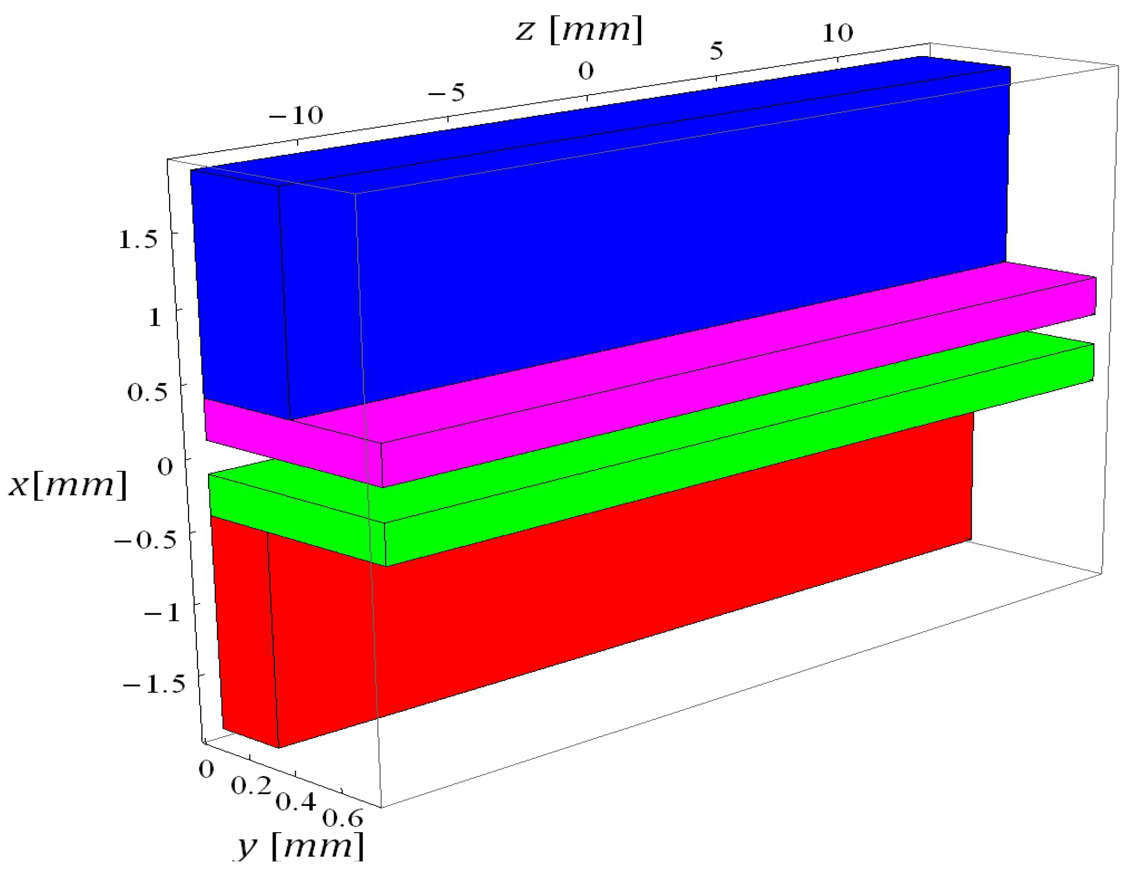
- Reduced dimensionality models which are predictable mechanistic models that feature reduced computational load yet retain higher accuracy of current density predictions. These are typically 2D models (e.g., [28], the 2D model in [29]) modelling straight channel fuel cell configurations (such as depicted in Figure 1) solving governing equations in the plane that is parallel to the gas flow and perpendicular to the membrane (e.g., green plane in Figure 1). Further simplification of 2D models leads to the so called 1D + 1D (e.g., [30]) models where mathematical treatment of the dimension that runs along direction of gas flow addresses only the most dominant physical phenomena (e.g., mass transport via bulk gas flow in channel). Applying these 2D models to a fuel cell geometry such as presented in Figure 1 leads to certain systematic discrepancies since the area through which mass is exchanged between the gas diffusion layer (GDL) and the channel is considerably smaller than the area where mass is exchanged between the membrane and the GDL. To compensate for this discrepancy some models employ additional correction parameters, obtained through fitting results of full 3D CFD models or experimental data, yielding pseudo 3D models (e.g., [31,32] and Sherwood number adjusted 2D model in [29]). An alternative to this pseudo 3D modelling is the so called 2D + 1D approach (as found in [29]) where the physical phenomena are fully addressed in the plane perpendicular to the gas flow and the reduced treatment of the 1D + 1D approach is used in the direction of gas flow.
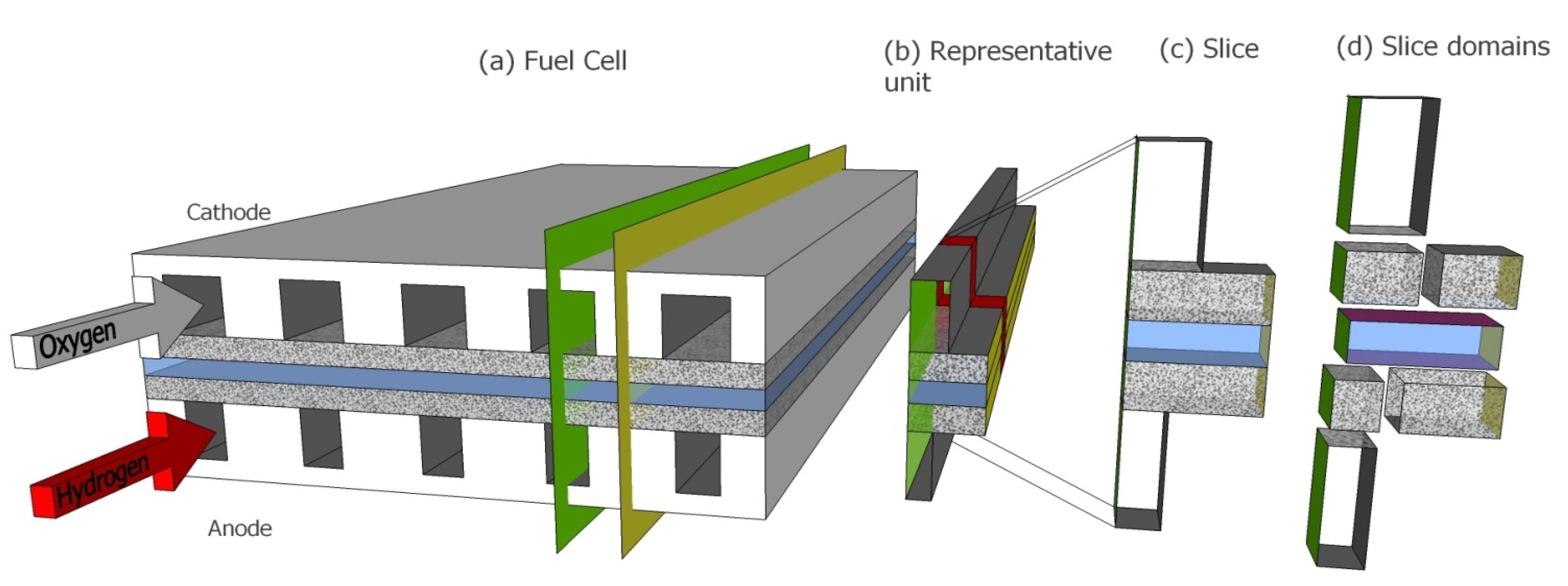
- The HAN-ST principle extended to more general realistic straight parallel channel FC geometries by devising the 2D analytic solution on a jigsaw puzzle of multiple domains and
- An electrochemistry sub-model efficiently coupled to this extended HAN-ST sub-model.
2. Model Assumptions and Geometry
- A steady state solution of the problem is sought.
- The problem is isothermal meaning a constant uniform temperature is assumed for the whole fuel cell and no energy equation is calculated.
- The gases are treated as ideal.
- There is no liquid water in GDLs and Channels.
- Pressure variations are small enough that constant pressure is assumed in gas equations and the gas flow is assumed incompressible over the whole fuel cell. This is justifiable due to very small pressure variations in the fuel cell owing to the short straight channel geometry.
- The diffusion system is always bi-componential (either oxygen and water vapour or hydrogen and water vapour) with a constant binary diffusion coefficient.
- The effective (macroscopic) diffusion constant used in GDL is the diffusion constant for empty space (which applies in the channel) divided by the tortuosity of GDL.
- Diffusion in gas in the direction of channel gas-flow is neglected due to the large aspect ratio of the relevant fuel cell dimensions.
- In GDL there is no convective transport in the direction of channel gas flow. The very small pressure drop from inlet to outlet produces only negligible convective flow in the GDL in the direction along channel length.
- The flow in channels is laminar.
- XI.
- There is no gas crossover in the membrane. Thus water is the only species transported through the membrane besides protons.
- XII.
- The mobility of both water molecules and protons (in form of hydronium ions) at a given point in membrane are linearly proportional to the membrane water content at that point.
- XIII.
- Species transport within the membrane only occurs in the direction perpendicular to the membrane sheet.
- XIV.
- The average number of water molecules dragged by the electro-osmotic pull of each proton is an independent constant.
- XV.
- The concentration of mobile protons is constant within the whole membrane. This is due to the humidification of membrane being always sufficiently high that full or close to full proton dissociation can be assumed.
- XVI.
- The membrane water content at the membrane/gas boundary is in equilibrium with water vapour concentration in the gas.
- XVII.
- Only the electrochemical kinetics of oxygen reduction on the cathode catalyst is considered. The electrochemical kinetics of hydrogen oxidation on the anode catalyst is much faster and its contribution to the over-potential is several orders of magnitude smaller and thus neglected.
- XVIII.
- The catalyst layer is infinitely thin and characterised by an effective exchange current density as current per unit area [A/m2].
- XIX.
- The electrical resistance of the GDL is neglected and uniform constant electrical potential is assumed within the whole GDL.
3. Governing Equations
3.1. Gas Part
3.1.1. GDL Domains
- -
- the first, defined by Equation (A31), deals with species transport induced by convective transport along the coordinate, and thus does not apply to GDL domains;
- -
- the second, defined by Equation (A41), deals with species transport induced by the boundary conditions at the boundaries of the 2D computational domains and applies also to GDL domains.
3.1.2. Channel Domain
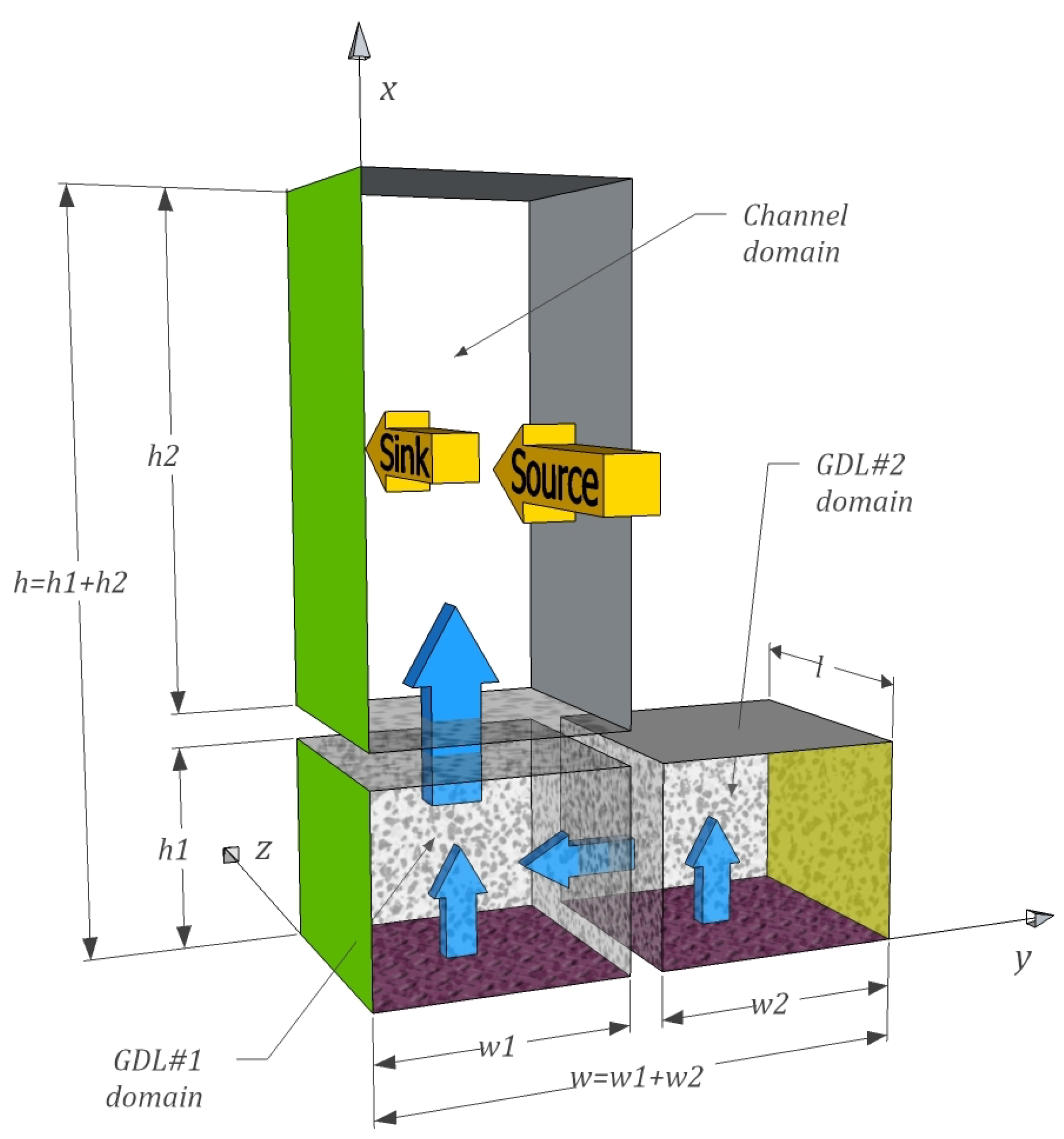
- The total molar gas flow and the molar flux of water vapour between the channel and the GDL, schematically represented with the wider vertical blue arrow in Figure 2, manifest as boundary conditions:and:where denotes the position at the GDL/channel boundary and is the gas velocity component perpendicular to the boundary between GDL#1 and channel evaluated at that boundary.
- Analogous to conditions (15) and (16) there is no flux through walls and across the symmetry plane, leading to the boundary condition for the other three edges:and:where , and denote the position at the two walls and the symmetry plane respectively.
3.2. MEA Part

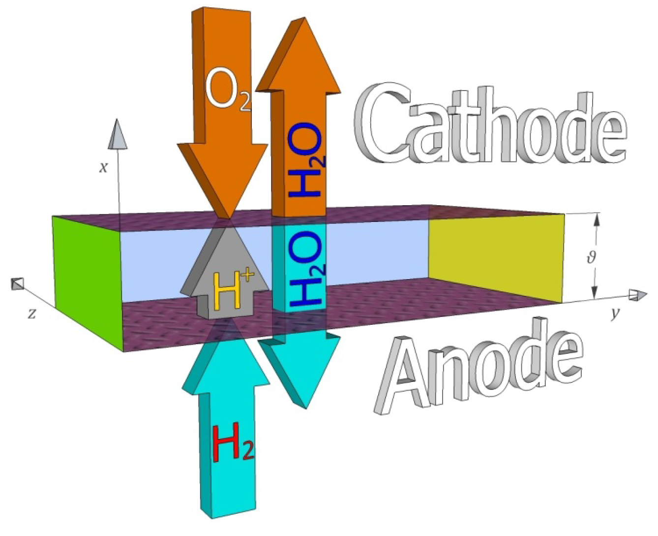
- species transport across the membrane (water molecules and hydronium ions represented by the cyan “H2O” and the gray “H+” arrow in Figure 3);
- species production and consumption by the electrochemical reactions on the catalysts that are on the top and bottom boundary of the MEA domain as observed in Figure 3.
3.2.1. Species Transport across Membrane
3.2.2. Electrochemical Reaction Kinetics
3.3. Coupling of General Solutions in Domains

| GDL domains | ||
|---|---|---|
| Species transport | Governing equation | |
| Boundary conditions | ||
| Velocity profile | Governing equation | |
| Boundary conditions | ||
| Channel domain | ||
| Species transport | Governing equation | |
| Boundary conditions | ||
| Velocity profile | Governing equation | |
| Boundary conditions | ||
| MEA domain | ||
| Species transport | Governing equation | |
| Boundary conditions | ||
| Electrochemical kinetics | ||
3.4. Solution for the Whole Cell
3.4.1. 2D Analytic Solution for a Slice
- Within a slice the coupling of two domains at their common boundary via the coupling conditions described in Section 3.3 is, on the level of eigen functions, manifested in algebraic coupling of the two sets of Fourier coefficients pertaining to the two linear combinations of harmonics in the two domains as described in Section A.3.1 of Appendix A.
- Coupling to the neighbour upstream slice via the two source terms in cathode and anode channel domain fully defines the solution for a slice (at a given operational voltage). Coupling to the downstream slice has no influence on the solution in the slice in question since sink terms are fully defined by concentration distribution in the two channel domains and are, due to assumption VIII, not influenced by the conditions in the neighbour downstream slice. Source terms, defined in Equation (28), also come in the form of a linear combination of eigen functions [Equation (A27)] thus the seven linear combinations that constitute the full solution for a slice are an algebraic function of the two linear combinations of the two source terms.
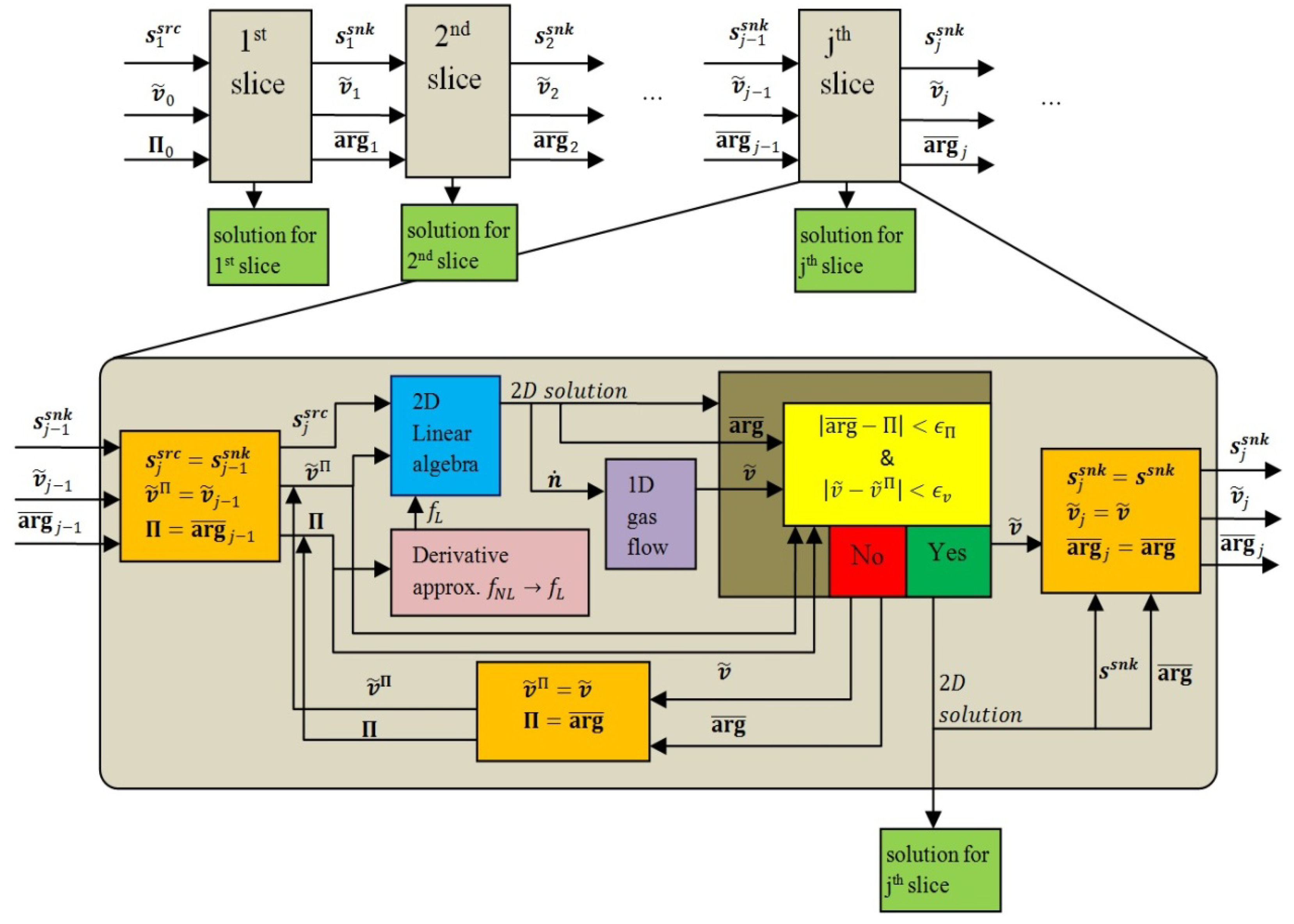
3.4.2. 1D Gas-Flow Equations
3.5. HAN Concept Extendibility
4. Simulation Setup
| Parameter | Symbol | Value |
|---|---|---|
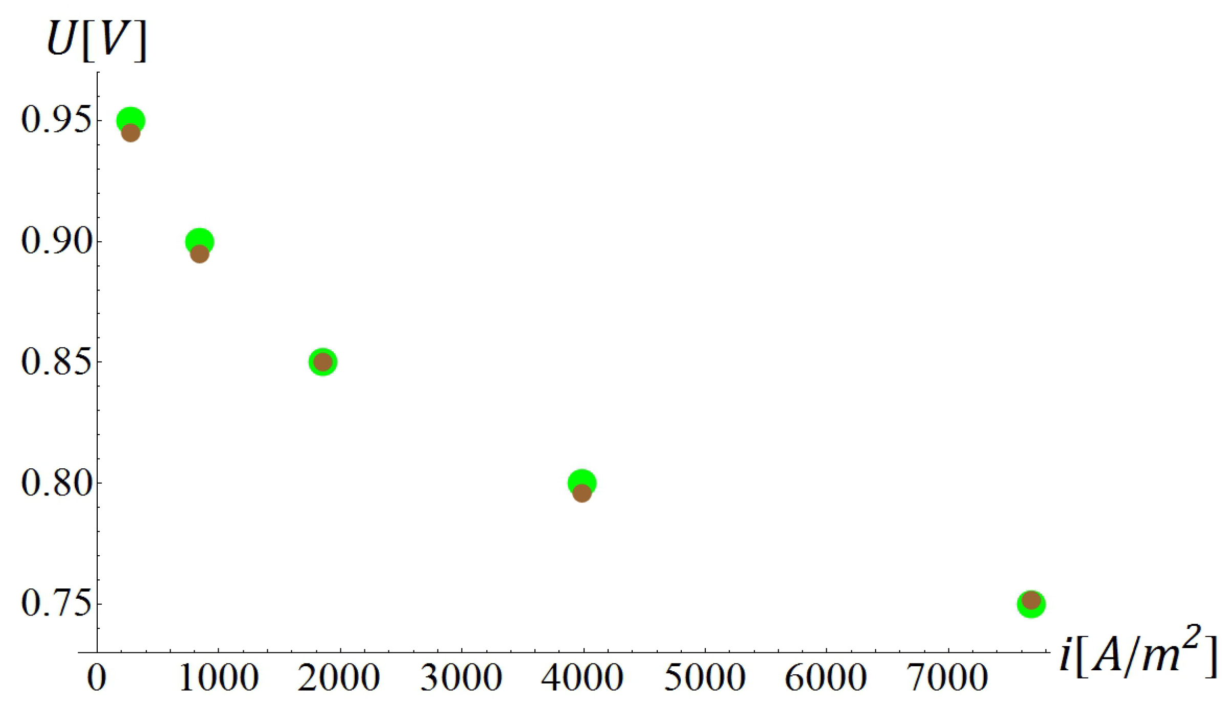
| Operational voltage | 0.95 V, 0.9 V, 0.85 V, 0.8 V, 0.75 V | |
| Temperature | 343.15 K | |
| Pressure * | 1.0 × 10⁵ Pa | |
| Inlet gas velocity (anode and cathode) | 0.3 m/s | |
| saturated water vapour partial pressure at 343.15 K | 3.12 × 10⁴ Pa | |
| Inlet gas relative humidity (anode and cathode) | 0.5 | |
| H2O(g)/O2 binary diffusion coeff. (at 343.15 K) ** | 3.01 × 10⁻⁵ m2/s | |
| H2O(g)/H2 binary diffusion coeff. (at 343.15 K) ** | 1.12 × 10⁻⁴ m2/s | |
| Coefficient of proportionality to water content of water diffusion coefficient in membrane (at 343.15 K) | 2.1 × 10⁻⁷ m2/s | |
| Coefficient of proportionality to water content of proton diffusion coefficient in membrane (at 343.15 K) | 1.6 × 10⁻⁸ m2/s | |
| Membrane sulphonic group concentration | 1900 mol/m3 | |
| GDL gaseous phase volume fraction (anode and cathode) | 0.78 | |
| GDL tortuosity (anode and cathode) | 1.34 | |
| Cathode charge transfer coefficient | 0.855 | |
| Channel height (anode and cathode) | 1.5 × 10⁻³ m | |
| Half of anode channel width | 2.5 × 10⁻⁴ m | |
| Half of cathode channel width | 3.75 × 10⁻⁴ m | |
| GDL thickness (anode and cathode) | 2.85 × 10⁻⁴ m | |
| width of representative unit | 7.5 × 10⁻⁴ m | |
| length of Representative unit | 2.7 × 10⁻² m | |
| Membrane thickness | 3.5 × 10⁻⁴ m |

- In HAN3 only first 3 modes per each coordinate. (i.e., 3 modes along y and 3 modes along x coordinate) are taken into account in harmonics in each gas part computational domain.
- In HAN6 first 6 modes per each coordinate are taken into account in harmonics in each gas part computational domain.
- In HAN9 first 9 modes per each coordinate are taken into account in harmonics in each gas part computational domain.
5. Calibration and Results

5.1. Calibration

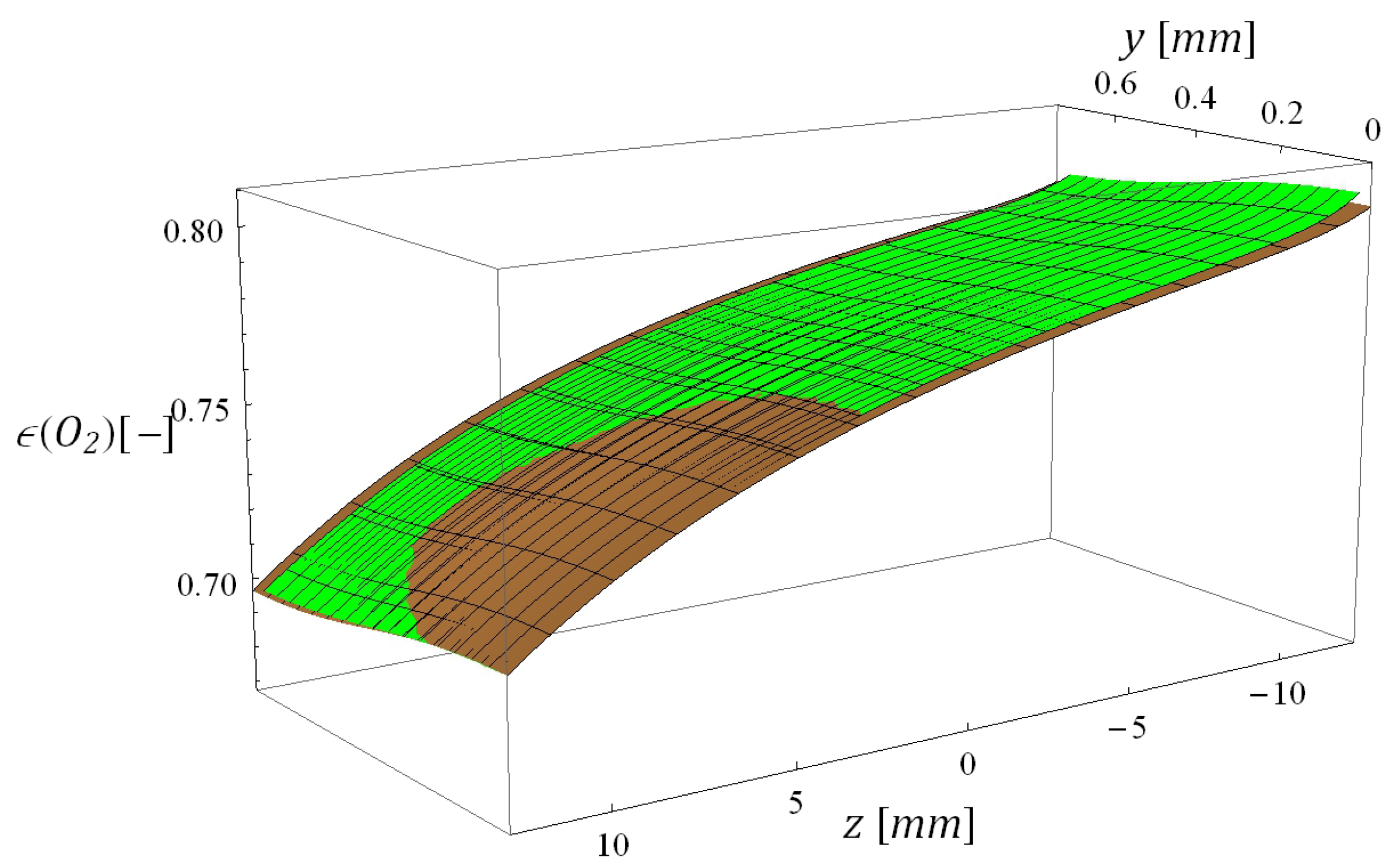
5.2. Plots of Comparative Results


5.3. Computational Times
| Model | Resolution | No. of iterations * | CPU cores used | CPU time (s) | Total time (s) |
|---|---|---|---|---|---|
| CFD(denser) | 34,560 vol. el. | 10,000 | 4 | 38,000 | 13,000 |
| CFD(coarser) | 4320 vol. el. | 5000 | 4 | 2400 | 640 |
| HAN3 | 3 modes | 1 | 1 | 0.85 | 0.85 |
| HAN6 | 6 modes | 1 | 1 | 3.7 | 3.7 |
| HAN9 | 9 modes | 1 | 1 | 6.0 | 6.0 |
6. Conclusions
- The 1D numerical treatment of gas flow;
- The analytic 2D solution for the species concentration profile in the plane perpendicular to the gas flow and
- The electrochemical sub-model.
Nomenclature
Symbols
Channel cross-sectional area | |
Velocity potential in channel domain | |
concentration in channel domain | |
water activity | |
Argument of a nonlinear function | |
Butler-Volmer function | |
Velocity potential in GDL#1 domain | |
concentration in GDL#1 domain | |
Water vapour concentration | |
Velocity potential in GDL#2 domain | |
concentration in GDL#2 domain | |
Membrane sulphonic group concentration | |
Concentration of dissociated protons in membrane | |
Total molar concentration of gas | |
catalyst surface concentration of reaction product | |
catalyst surface concentration of reactant | |
reference concentration | |
concentration of saturated water vapour | |
Gaseous binary diffusion constant | |
diffusion constant of protons in membrane | |
diffusion constant of water in membrane | |
coefficient of proportionality of proton diffusivity to water content | |
coefficient of proportionality of water diffusivity to water content | |
Faraday constant | |
Linearised nonlinear function | |
Nonlinear function | |
Either or | |
Sum of channel height and GDL thickness | |
GDL thickness | |
Channel height | |
Electric/proton current density | |
Cathode catalyst effective exchange current density | |
Molar flux of water | |
Molar flux of protons | |
Length of representative unit | |
Depth of slice | |
Index of modes along coordinate | |
Coordinate normal to boundary plane/index of modes along coordinate | |
Molar flux | |
Electroosmotic drag coefficient | |
Pressure | |
Gas constant/membrane ohmic resistance | |
Source or sink term for species concentration | |
time | |
Temperature | |
Velocity potential in plane | |
Velocity vector (3D) | |
Electric potential | |
Operational voltage | |
Membrane overpotential | |
Velocity | |
Average velocity | |
Sum of and | |
Width of GDL#1 domain | |
Width of GDL#2 domain | |
Coordinate perpendicular to membrane | |
Coordinate perpendicular to channel gas-flow and parallel to membrane | |
Coordinate parallel to direction of channel gas-flow | |
concentration defined in (A2) |
Greek Letters
Cathode catalyst electron transfer coefficient/any of | |
Velocity vector in plane (2D) | |
Membrane thickness | |
Volume fraction of non-solid space in GDL | |
Membrane water content | |
Eigen value of eigen function | |
Integration constant | |
Predictor value | |
Source or sink term for velocity potential | |
Dimensionless shape of velocity profile | |
Cathode Galvani potential | |
Cathode open circuit Galvani potential at reference conditions | |
Cathode open circuit Galvani potential at standard conditions | |
Eigen function for flow from boundary | |
Eigen function for channel flow terms | |
Ohmic function | |
Geometrical factor |
Superscripts or Subscripts
GDL#1 domain/argument 1 | |
GDL#2 domain/argument 2 | |
Anode | |
Bottom boundary | |
Channel domain | |
Either or | |
Cathode | |
diffusion from boundary | |
Gas diffusion layer | |
Hydrogen | |
Left boundary | |
Membrane domain | |
Number of modes taken into account | |
Oxygen | |
Previous (upstream) | |
Right boundary | |
Sink | |
Source | |
Top boundary | |
Water |
Conflicts of Interest
Appendix A
A.1. Gas Part
A.1.1. Diffusion Differential Equation
A.1.2. Eigen Functions
A.1.2.1. Eigen Functions for Channel Flow Terms
A.1.2.2. Eigen Functions for Flow from Boundary
A.1.2.3. Additional Conditions for Sum of all Contributions in a Domain
- Channel domain
- GDL#1 domain
- GDL#2 domain
A.2. MEA Domain
A.3. Coupling of Linear Combinations of Eigen Functions
- Couplings between domains of a slice that require continuity of water activity and molar fluxes and
- Couplings between channel domains in consecutive slices that require computing sink terms that serve as source terms in neighbour downstream slices.
A.3.1. Couplings between Domains of a Slice
- From channel domain side taking into account the definition of in Equation (A31):
- And from GDL#1 side taking into account the definition of in Equation (A41):
A.3.2. Coupling between Slices
A.4. Analytic 2D Solution for a Slice
Appendix B
References
- Hellman, H.L.; van den Hoed, R. Characterising fuel cell technology: Challenges of the commercialisation process. Int. J. Hydrog. Energy 2007, 32, 301–315. [Google Scholar] [CrossRef]
- Ly, H.; Birgersson, E.; Vynnycky, M. Fuel cell model reduction through the spatial smoothing of flow channels. Int. J. Hydrog. Energy 2012, 37, 7779–7795. [Google Scholar] [CrossRef]
- Haraldsson, K.; Wipke, K. Evaluating PEM fuel cell system models. J. Power Sources 2004, 126, 88–97. [Google Scholar] [CrossRef]
- Cheddie, D.; Munroe, N. Review and comparison of approaches to proton exchange membrane fuel cell modeling. J. Power Sources 2005, 147, 72–84. [Google Scholar] [CrossRef]
- Gurau, V.; Mann, J.A., Jr. A Critical overview of computational fluid dynamics multiphase models for proton exchange membrane fuel cells. SIAM J. Appl. Math. 2009, 70, 410–454. [Google Scholar] [CrossRef]
- Meng, H. A three-dimensional PEM fuel cell model with consistent treatment of water transport in MEA. J. Power Sources 2006, 162, 426–435. [Google Scholar] [CrossRef]
- Sivertsen, B.R.; Djilali, N. CFD-based modelling of proton exchange membrane fuel cells. J. Power Sources 2005, 141, 65–78. [Google Scholar] [CrossRef]
- Al-Baghdadi, M.A.R.S. Three-dimensional computational fluid dynamics model of a tubular-shaped ambient air-breathing proton exchange membrane fuel cell. J. Power Energy 2008, 222, 569–585. [Google Scholar] [CrossRef]
- Wang, Y.; Wang, C.Y. Ultra large-scale simulation of polymer electrolyte fuel cells. J. Power Sources 2006, 153, 130–135. [Google Scholar] [CrossRef]
- Campanari, S.; Manzolini, G.; de la Iglesa, F.G. Energy analysis of electric vehicles using batteries or fuel cells through well-to-wheel driving cycle simulations. J. Power Sources 2009, 186, 464–477. [Google Scholar] [CrossRef]
- Moore, R.M.; Hauer, K.H.; Ramaswamy, S.; Cunningham, J.M. Energy utilization and efficiency analysis for hydrogen fuel cell vehicles. J. Power Sources 2006, 159, 1214–1230. [Google Scholar] [CrossRef]
- Xue, X.; Smirnova, A.; England, R.; Sammes, N. System level lumped-parameter dynamic modeling of PEM fuel cell. J. Power Sources 2004, 133, 188–204. [Google Scholar] [CrossRef]
- Lee, C.; Yang, J. Modeling of the Ballard-Mark-V proton exchange membrane fuel cell with power converters for applications in autonomous underwater vehicles. J. Power Sources 2011, 196, 3810–3823. [Google Scholar] [CrossRef]
- Pathapati, P.R.; Xue, X.; Tang, J. A new dynamic model for predicting transient phenomena in a PEM fuel cell system. Renew. Energy 2005, 30, 1–22. [Google Scholar] [CrossRef]
- Moore, R.M.; Hauer, K.H.; Friedman, D.; Cunningham, J.; Badinnarayanan, P.; Ramaswamy, S.; Eggert, A. A dynamic simulation tool for hydrogen fuel cell vehicles. J. Power Sources 2005, 141, 272–285. [Google Scholar] [CrossRef]
- Boulon, L.; Agbossou, K.; Hissel, D.; Sicard, P.; Bouscayrol, A.; Pérad, M.C. A macroscopic PEM fuel cell model including water phenomena for vehicle simulation. Renew. Energy 2012, 46, 81–91. [Google Scholar] [CrossRef]
- Hatti, M.; Tioursi, M. Dynamic neural network controller model of PEM fuel cell system. Int. J. Hydrog. Energy 2009, 34, 5015–5021. [Google Scholar] [CrossRef]
- Hinaje, M.; Raël, S.; Noiying, P.; Nguyen, D.A.; Davat, B. An equivalent electrical circuit model of proton exchange membrane fuel cells based on mathematical modelling. Energies 2012, 5, 2724–2744. [Google Scholar] [CrossRef]
- Tirnovan, R.; Giurgea, S.; Miraoui, A.; Cirrincione, M. Corresponding author contact information, Surrogate model for proton exchange membrane fuel cell (PEMFC). J. Power Sources 2008, 175, 773–778. [Google Scholar] [CrossRef]
- Zhong, Z.-D.; Zhu, X.-J.; Cao, G.-Y. Modeling a PEMFC by a support vector machine. J. Power Sources 2006, 160, 293–298. [Google Scholar] [CrossRef]
- Gurau, V.; Barbir, F.; Liu, H. An analytical solution of a half-cell model for PEM fuel cells. J. Electrochem. Soc. 2000, 147, 2468–2477. [Google Scholar] [CrossRef]
- Maggio, G.; Recupero, V.; Pino, L. Modeling polymer electrolyte fuel cells: An innovative approach. J. Power Sources 2001, 101, 275–286. [Google Scholar] [CrossRef]
- Springer, T.E.; Zawodzinski, T.A.; Gottesfeld, S. Polymer electrolyte fuel cell model. J. Electrochem. Soc. 1991, 138, 2334–2342. [Google Scholar] [CrossRef]
- Tirnovan, R.; Giurgea, S.; Miraoui, A.; Cirrincione, M. Proton exchange membrane fuel cell modelling based on a mixed moving least squares technique. Int. J. Hydrog. Energy 2008, 33, 6232–6238. [Google Scholar] [CrossRef]
- Iftikar, M.U.; Riu, D.; Druart, F.; Rosini, S.; Bultel, Y.; Retière, N. Dynamic modeling of proton exchange membrane fuel cell using non-integer derivatives. J. Power Sources 2006, 160, 1170–1182. [Google Scholar] [CrossRef]
- Wohr, M.; Bolwn, K.; Schnurnberger, W.; Fischer, M.; Neubrand, W.; Eigenberger, G. Dynamic modeling and simulation of a polymer membrane fuel cell including mass transport limitation. Int. J. Hydrog. Energy 1998, 23, 213–218. [Google Scholar] [CrossRef]
- Xue, X.D.; Cheng, K.W.E.; Sutanto, D. Unified mathematical modelling of steady-state and dynamic voltage—Current characteristics for PEM fuel cells. Electrochim. Acta 2006, 52, 1135–1144. [Google Scholar] [CrossRef]
- Ee, S.L.; Birgersson, E. Two-dimensional approximate analytical solutions for the direct liquid fuel cell. J. Electrochem. Soc. 2011, 158, 1224–1234. [Google Scholar] [CrossRef]
- Kim, G.; Sui, P.C.; Shah, A.A.; Djilali, N. Reduced-dimensional models for straight-channel proton exchange membrane fuel cells. J. Power Sources 2010, 195, 3240–3249. [Google Scholar] [CrossRef]
- Esmaili, Q.; Ranjbar, A.A.; Abdollahzadeh, M. Numerical simulation of a direct methanol fuel cell through a 1D + 1D approach. Int. J. Green Energy 2013, 10, 190–204. [Google Scholar] [CrossRef]
- Ling, C.Y.; Ee, S.L.; Birgersson, E. Three-dimensional approximate analytical solutions for direct liquid fuel cells. Electrochimica Acta 2013, 109, 305–315. [Google Scholar] [CrossRef]
- Chang, P.; Kim, G.-S.; Promislow, K.; Wetton, B. Reduced dimensional computational models of polymer electrolyte membrane fuel cell stacks. J. Comput. Phys. 2007, 223, 797–821. [Google Scholar]
- Tavčar, G.; Katrašnik, T. A computationally efficient hybrid 3D analytic-numerical approach for modelling species transport in a proton exchange membrane fuel cell. J. Power Sources 2013, 236, 321–340. [Google Scholar] [CrossRef]
- Berg, P.; Promislow, K.; Pierre, J.; Stumper, J.; Wetton, B. Water management in PEM fuel cells. J. Electrochem. Soc. 2004, 151, 341–353. [Google Scholar] [CrossRef]
- Cussler, E.L. Diffusion: Mass Transfer in Fluid Systems, 3rd ed.; Cambridge University Press: Cambridge, UK, 2009. [Google Scholar]
- O’Hayre, R.; Cha, S.-W.; Colella, W.G.; Prinz, F.B. Fuel Cell Fundamentals; Wiley: Hoboken, NJ, USA, 2009. [Google Scholar]
- Wang, Y.; Feng, X. Analysis of reaction rates in the cathode electrode of polymer electrolyte fuel cell I. Single-layer electrodes. J. Electrochem. Soc. 2008, 155, 1289–1295. [Google Scholar] [CrossRef]
- He, R.; Qingfeng, L.; Xiao, G.; Bjerrum, N.J. Proton conductivity of phosphoric acid doped polybenzimidazole and its composites with inorganic proton conductors. J. Membr. Sci. 2003, 226, 169–184. [Google Scholar] [CrossRef]
- Qingfeng, L.; Hjuler, H.A.; Bjerrum, N.J. Phosphoric acid doped polybenzimidazole membrane: Physiochemical characterisation and fuel cell applications. J. Appl. Electrochem. 2001, 31, 773–779. [Google Scholar] [CrossRef]
- Fink, C.; Fouquet, N. Three-dimensional simulation of polymer electrolyte membrane fuel cells with experimental validation. Electrochim. Acta 2011, 56, 10820–10831. [Google Scholar] [CrossRef]
- Fouquet, N.; Fink, C.; Tatschl, R. 3D Modeling of PEM Fuel Cell with AVL Fire. In Proceedings of the AVL Advanced Simulation Technologies International User Conference 2011, Graz, Austria, 28–30 June 2011.
- AVL LIST GmbH. Fire v20111—Electrification & Hybridization. In AVL FIRE Version 2011 User Manual; Document No. 08.0205.2011; AVL LIST GmbH: Graz, Austria, 2011. [Google Scholar]
© 2013 by the authors; licensee MDPI, Basel, Switzerland. This article is an open access article distributed under the terms and conditions of the Creative Commons Attribution license (http://creativecommons.org/licenses/by/3.0/).
Share and Cite
Tavčar, G.; Katrašnik, T. An Innovative Hybrid 3D Analytic-Numerical Approach for System Level Modelling of PEM Fuel Cells. Energies 2013, 6, 5426-5485. https://doi.org/10.3390/en6105426
Tavčar G, Katrašnik T. An Innovative Hybrid 3D Analytic-Numerical Approach for System Level Modelling of PEM Fuel Cells. Energies. 2013; 6(10):5426-5485. https://doi.org/10.3390/en6105426
Chicago/Turabian StyleTavčar, Gregor, and Tomaž Katrašnik. 2013. "An Innovative Hybrid 3D Analytic-Numerical Approach for System Level Modelling of PEM Fuel Cells" Energies 6, no. 10: 5426-5485. https://doi.org/10.3390/en6105426
APA StyleTavčar, G., & Katrašnik, T. (2013). An Innovative Hybrid 3D Analytic-Numerical Approach for System Level Modelling of PEM Fuel Cells. Energies, 6(10), 5426-5485. https://doi.org/10.3390/en6105426