Evolution of Hydrate Dissociation by Warm Brine Stimulation Combined Depressurization in the South China Sea

Abstract

To evaluate the gas production performance of the hydrate accumulations in the South China Sea, a numerical simulation with warm brine stimulation combined depressurization has been conducted. A dual horizontal well system is considered as the well configuration in this work. In order to reduce energy input and improve energy utilization, warm brine (<30 °C) instead of hot brine (>50 °C) is injected into the reservoir for hydrate dissociation. The effect of the intrinsic permeability of the hydrate reservoir, the salinity and the temperature of the injected brine to gas hydrate exploitation have been investigated. The numerical simulation results indicate that the average gas production rate Q_avg is about 1.23 × 10⁵ ST m³/day for the entire hydrate deposit, which has the same order of magnitude compared with the commercially viable production rate. The injected brine can be pumped out from the upper production well directly after the hydrate between the two wells is dissociated completely. Thus, the effective region of heat and inhibitor stimulation is limited. The sensitivity analyses indicate that the dissociation rate of hydrate can be enhanced by increasing the temperature of the injected brine and raising the salinity of the injected brine. The parametric study of permeability shows that the hydrate of the reservoir with the larger permeability has a higher dissociation rate.

1. Introduction

1.1. Background

Natural gas hydrates are crystalline solids composed of water and gas, in which the gas molecules (guests) are trapped in the water cavities (hosts). The water cavities are comprised of hydrogen-bonded water molecules. Methane, ethane, propane, and carbon dioxide are recognized as the typical natural gas molecules [1]. Given the restricted conventional fossil fuel reserves and the ever-increasing global energy demand, natural gas hydrate is regarded as a potential energy resource because the current estimated amount of natural gases encaged in gas hydrate is vast [2]. It is generally accepted that gas hydrate exists widely in oceanic sediments and the permafrost region where the conditions of high pressure and low temperature are favorable for its formation and stability [3].

The study on how to decompose the solid hydrate economically and effectively is a crucial issue in gas hydrate exploitation. The major methods of hydrate dissociation include depressurization [4,5], thermal stimulation [6], and the use of thermodynamic inhibitors [7]. On account of the fact that each approach has its pros and cons, the combined utilization of depressurization and thermal stimulation has been proven to be favorable for hydrate dissociation [8]. Hot brine stimulation combines the advantages of thermal stimulation and inhibitor stimulation. Li et al. [9] indicated that the hot brine stimulation experiment could obtain a higher energy efficiency than that using hot water stimulation. Subsequently, Li et al. [10] further indicated that the hydrate dissociation rate increased with the increase of salinity. Recently, Moridis et al. [11] showed that the dual horizontal well system is better than the single horizontal well layout because of preferable heat transference. Much research in recent years has focused on hydrate dissociation under hot water stimulation, but few studies have investigated warm brine stimulation, especially with dual horizontal wells.

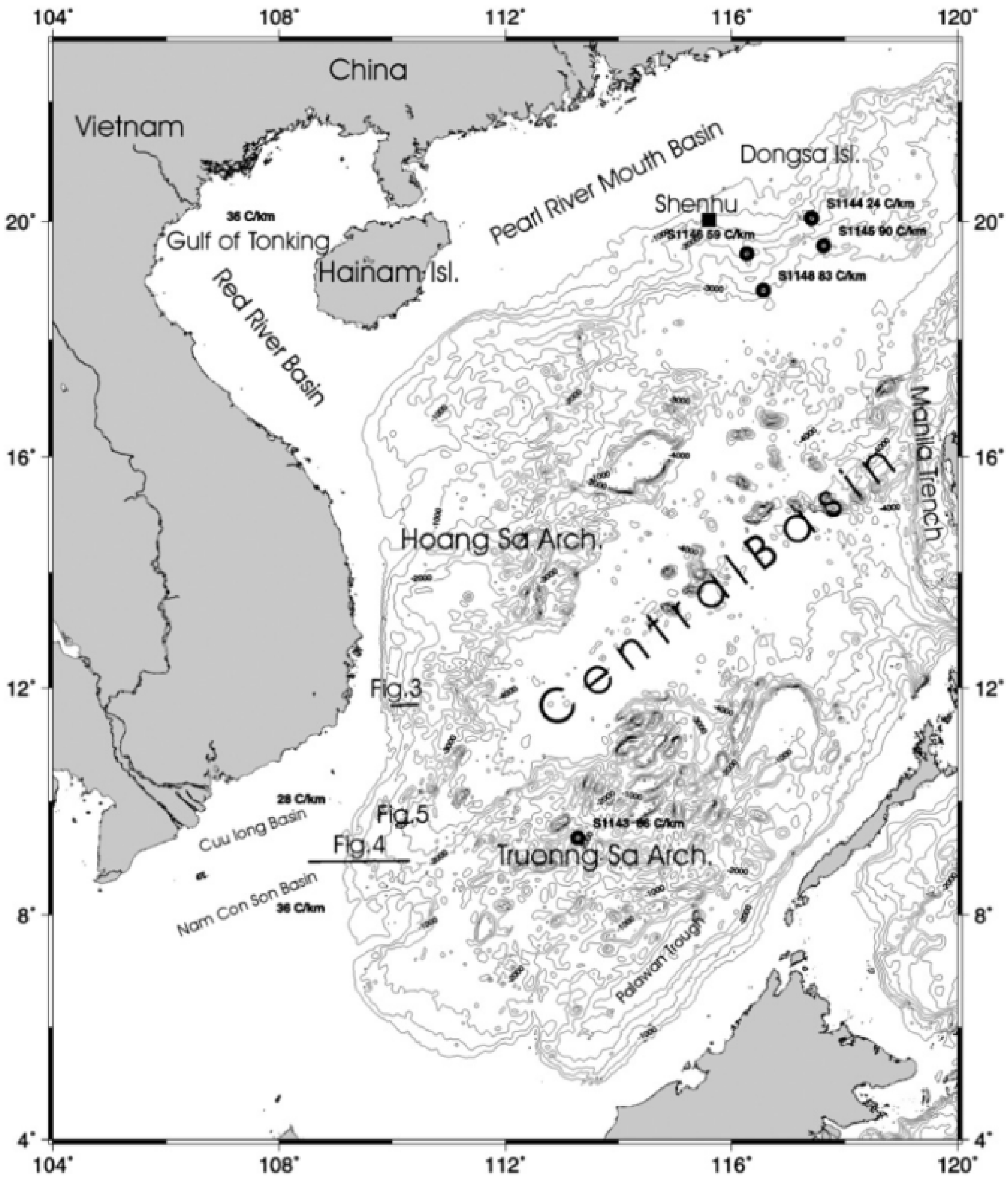
1.2. Oceanic Hydrates and the Hydrates in the South China Sea

As the oceans comprise 70% of the Earth’s surface, the oceanic hydrate accumulations constitute approximately 99% of the total gas hydrate resource [2]. The Gulf of Mexico and the Nankai Trough are considered as two models for evaluating the oceanic gas hydrate prospects [12]. Japan obtained gas from the oceanic hydrates by depressurization in the Nankai Trough in March of 2013 [13], which was the world’s first successful production of gas from hydrate reservoir at the bottom of the ocean. In the northern Gulf of Mexico, a logging-while-drilling expedition was conducted in April and May of 2009 [14]. The drilling tests showed that high S_H (from 50% to 90%) hydrate samples were acquired in two wells in Walker Ridge 313 and two in Green Canyon 955. Because of the limited long-term production data from hydrate-bearing accumulations, numerical simulation has been regarded as an effective way in evaluating gas production [15].

Nowadays, research results indicate that abundant gas hydrate exists in the continental slope of the South China Sea (SCS, Figure 1) [16,17,18]. In May, 2007, gas hydrate samples were discovered in the Shenhu Area of the SCS during the scientific expedition carried out by the China Geological Survey.

Figure 1. Map of the South China Sea [16].

Figure 1. Map of the South China Sea [16].

Li et al. [19] and Su et al. [20] established their models based on the measurement data from different sites in the Shenhu Area. They both used the huff and puff method to investigate the gas production performance from the hydrate sediments with a horizontal well and a vertical well respectively. The results demonstrate that the gas production relies on the initial intrinsic permeability, the temperature, the hydrate saturation of the Hydrate-Bearing Layer (HBL), and the temperature of the well. However, the gas production rates are several orders of magnitude less than acceptable standards of commercial viable gas production.

1.3. Objectives

This study aims to evaluate the gas production potential from hydrate accumulations in the SCS by numerical simulation. A model of gas hydrate reservoir is established from the available data in the SCS [16,21,22]. The well configuration is the dual horizontal wells in this study, like the work of Moridis et al., the lower horizontal well is set as the injection well and the upper one is the production well. In addition, the warm brine (<30 °C) instead of hot brine (>50 °C) is applied in this work for improving energy utilization. The gas production of the hydrate reservoir is investigated by combining the depressurization, the thermal stimulation, and the inhibitor stimulation. The sensitivities of gas production to the injected temperature, the salinity of the injected brine, and the intrinsic permeability of the hydrate reservoir are also investigated.

2. Production Schemes and Well Design

2.1. Dissociation Method

Moridis et al. [23] reported that the Class 1 hydrate deposit was characterized by a HBL and an underlying two-phase fluid zone with free gas. Similarly, the Class 2 hydrate deposit consists of a HBL and an underlying zone of mobile water. The hydrate accumulation in the SCS is similar to the Class 3 deposit which involves only a HBL without underlying mobile fluid zones, and this kind of hydrate reservoir is regarded as “challenging” for gas production [24].

Depressurization has been widely used in gas hydrate studies for its technical viability and economic advantage [4,25]. Konno et al. [26] employed the numerical simulator MH21-HYDRES to evaluate the gas productivity of the four different kinds of hydrate reservoir by the depressurization method with a single vertical well. The results showed that depressurization was the most feasible technique in the Class 1 hydrate reservoir. Whereas the depressurization-induced method was unattractive for the Class 3 hydrate reservoir because of the absence of a free gas zone underneath the HBL. Earlier studies verified that the combined utilization of depressurization and thermal stimulation was favorable for gas production. However, simple hot water injection seemed to be ineffective due to the energy loss [23]. In this work, the gas production is conducted by combining warm brine stimulation and depressurization with dual horizontal wells.

2.2. Well Configuration

The investigation of Moridis et al. [27] indicated that the utilization of a horizontal well resulted in a dramatic increase of gas production from Class 2 and the Class 3 reservoirs compared with vertical wells. Thus a dual horizontal wells in the same vertical plane layout was applied in this study. The warm brine is injected into the lower horizontal well and the fluids are produced from the upper one under constant pressure conditions.

In this model, the distance between two wells is 20 m (shown in Figure 2a). The radius r_W of the wells are both 0.1 m. There are 12 grooves located along the circumference of the wells [28]. The porosity of the wellbores is assumed to be 1.0. The permeability k and the capillary pressure P_cap are set as 5.0 × 10⁻⁹ m² (5000 Darcies) and 0, respectively [19].

Figure 2. (a) Schematic of the marine hydrate reservoir in the South China Sea; (b) The corresponding 2-D hybrid mesh.

Figure 2. (a) Schematic of the marine hydrate reservoir in the South China Sea; (b) The corresponding 2-D hybrid mesh.

3. Numerical Models and Simulation Method

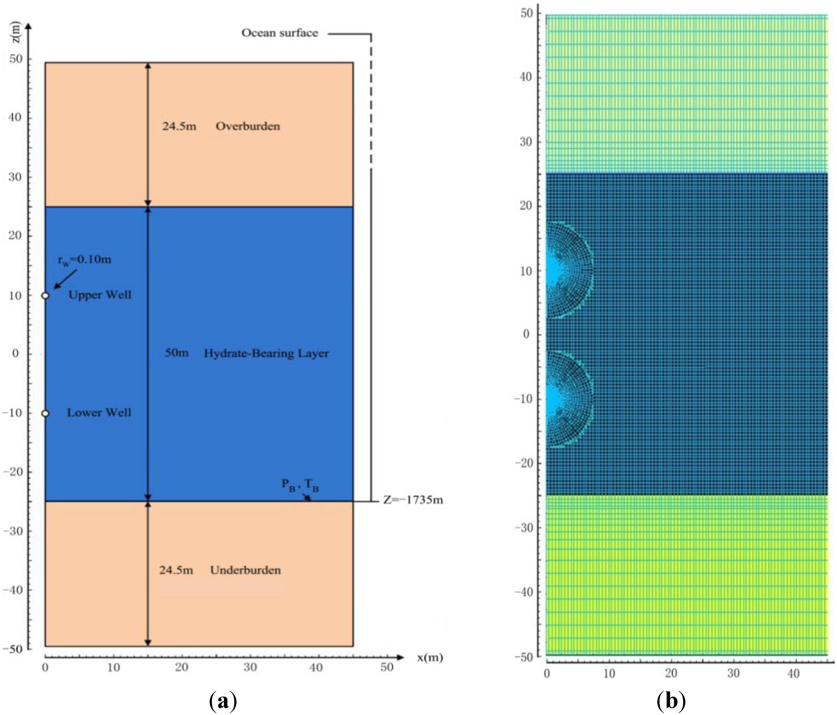
3.1. Geometry, Domain Discretization, and System Properties

Both the serial and parallel versions of the TOUGH+HYDRATE code [29,30] are applied in this study to perform the numerical simulation. In order to investigate the dissociation performance of the oceanic hydrate, the geologic parameters of this study is in accordance with the hydrate accumulations of the SCS. It is necessary to make reasonable estimations of the media properties since the field measurement data are quite limited. In this model, methane is assumed to be the only hydrate-forming gas.

The geometry and the configuration of the hydrate deposit with two parallel horizontal wells are shown in Figure 2a. The 50 m-thick HBL is located in the middle of the deposit. On the top of the HBL, a permeable overburden exists, and a permeable underburden lies under the HBL as well, which allows fluids flow and heat exchange in them. The thickness of the overburden and underburden both are 24.5 m, which are sufficient to permit accurate heat exchange, mass exchange, and pressure transfer in the hydrate accumulation. As seen in Figure 2, the total thickness of the whole domain simulated in this study is 99 m. In order to minimize the gas escape from the overburden and underburden, the two parallel wells are situated at z = 10 m and z = −10 m, respectively. This work set a simulation region of 0 ≤ x ≤ 45 m which indicates a well spacing of 90 m for symmetry, and there is no heat and mass flow at x = 0 and x = 45 m.

As shown in Figure 2b, a 2-D hybrid mesh (y = 1 m) is applied to conduct the simulation. This model can describe the performance of the entire 1000 m-long well. The mesh includes 12,228 elements, and 12,008 of them are active elements. The inactive elements belong to the boundary and steel gridblocks. The overburden and underburden are set as inactive boundary cells which meet constant temperature and pressure. For the sake of accurate prediction, Δz is finely discretized to be less than 0.5 m along the z axis in the top of the underburden, the HBL, and the bottom of the overburden. And the discretization far from the HBL becomes coarse. The regions around the horizontal wells are discretized to be pretty fine in order to describe the temperature and pressure precisely. The area of r < 7.5 m around the two wells are discretized into refined cylindrical meshes to accurately capture the complex physical and chemical processes. The first cylindrical layer (r = 0.1 m) has six gridblocks standing for the grooves of the well, and the remaining ones are the impermeable steel elements representing the wall of the well. The warm brine is injected into the HBL at a constant rate Q_inj from the six gridblocks which act as source terms in the injection well, while the six gridblocks in the upper well perform as sink terms. The discretization in the core of the circle is very fine, but it gets coarser in the direction of the radius. Supposing the hydrate dissociation with inhibitors in equilibrium state [29], the number of the coupled equations in this simulation is 48,032, which is from multiplying by 12,008 (active cells) and 4 (the equations of per cell include the mass balance equations of gas, water and salt, as well as the energy balance equation [31,32]).

3.2. Initial Conditions.

According to the available data [33], the depth of seawater H, the geothermal gradient G, and the salinity of the seawater X_S are selected as 1500 m, 45 K/km, and 3.50%, respectively. The remaining parameters used in this work are shown in Table 1.

Since the actual temperature and pressure measurements are unavailable, the T- and P-distribution of the system are estimated by the following methods. On the basis of the field measurements [16,21,22], the temperature of the sea floor T₀ is selected as 277.15 K. Then the T-distribution of the whole system including the temperatures T_T (at the top of the HBL) and T_B (at the bottom of the HBL, at z = −1735 m) are estimated in the light of the two basic parameters (T₀ and G). The initial temperature of T_B is 288.28 K (shown in Table 1). Afterwards, the hydrate pressure and temperature (P-T) equilibrium curve is employed to determine the lower restriction of P_B at the bottom of the HBL for keeping the steady state of the initial HBL. In this study, P_B is 18.25 MPa which is initialized a bit higher than the equilibrium pressure to guarantee the hydrate stability. Such system is easy to destabilize under thermal stimulation or depressurization [19].

Finishing initializing the P and T distributions in each gridblock (shown in Figure 2b), the other initial conditions, such as the saturation of gas (S_G), the saturation of water (S_A), and the salinity of brine (X_S) in the reservoir, can be achieved by another short simulation. As displayed in Table 1, the S_H and the S_A in the HBL, and the S_A of the overburden and underburden are 0.451, 0.549, and 1.0, respectively, which means no free gas existing in the whole system. The salinity of water in the model is 0.350. After completing initialization, any condition of the entire system will keep unchangeable unless a disturbance from outside occurs.

Table 1. Physical properties and simulation models in marine deposit of the South China Sea.

Parameter	Value	Parameter	Value
Thickness of HBL	50 m	Capillary pressure model [34]	Pcap = − P01 [(S*)−1/λ − 1] 1−λ S* = (SA − SirA)/(SmxA − SirA)
Thickness of OB and UB	24.5 m	SirA	0.29
Position of HBL below the ground	160.5 m	λ	0.45
distance between two wells	20 m	P01	105 Pa
Initial PB and TB (at base of HBL)	18.25 MPa, 288.28 K	Relative permeability Model	krA = (SA*)n krG = (SG*)nG SA* = (SA − SirA)/(1 − SirA) SG* = (SG − SirG)/(1 − SirA)
Gas composition	100% CH4	P01	105 Pa
Composite thermalconductivity model [29,35]	kΘC = kΘRD + (SA1/2 + SH1/2 ) (kΘRW − kΘRD) + ϕSIkΘI	Relative permeability Model	krA = (SA*)n krG = (SG*)nG SA* = (SA − SirA)/(1 − SirA) SG* = (SG − SirG)/(1 − SirA)
		n	3.572
		nG	3.572
Sea floor temperature T0	277.15 K	Relative permeability Model	krA = (SA*)n krG = (SG*)nG SA* = (SA − SirA)/(1 − SirA) SG*= (SG − SirG)/(1 − SirA)
Geothermal gradient G	0.045 K/m
Water salinity (mass fraction)	3.50%
Intrinsic permeability kx = ky= kz (HBL, OB & UB)	7.5 × 10−14 m2 (= 0.075 mD)	n	3.572
		nG	3.572
Porosity ϕ (all formations)	0.40	SirG	0.05
Initial hydrate saturation	SH = 0.451	SirA	0.30

Table 1. Physical properties and simulation models in marine deposit of the South China Sea.

Parameter	Value	Parameter	Value
Thickness of HBL	50 m	Capillary pressure model [34]	Pcap = − P01 [(S*)−1/λ − 1] 1−λ S* = (SA − SirA)/(SmxA − SirA)
Thickness of OB and UB	24.5 m	SirA	0.29
Position of HBL below the ground	160.5 m	λ	0.45
distance between two wells	20 m	P01	105 Pa
Initial PB and TB (at base of HBL)	18.25 MPa, 288.28 K	Relative permeability Model	krA = (SA*)n krG = (SG*)nG SA* = (SA − SirA)/(1 − SirA) SG* = (SG − SirG)/(1 − SirA)
Gas composition	100% CH4	P01	105 Pa
Composite thermalconductivity model [29,35]	kΘC = kΘRD + (SA1/2 + SH1/2 ) (kΘRW − kΘRD) + ϕSIkΘI	Relative permeability Model	krA = (SA*)n krG = (SG*)nG SA* = (SA − SirA)/(1 − SirA) SG* = (SG − SirG)/(1 − SirA)
		n	3.572
		nG	3.572
Sea floor temperature T0	277.15 K	Relative permeability Model	krA = (SA*)n krG = (SG*)nG SA* = (SA − SirA)/(1 − SirA) SG*= (SG − SirG)/(1 − SirA)
Geothermal gradient G	0.045 K/m
Water salinity (mass fraction)	3.50%
Intrinsic permeability kx = ky= kz (HBL, OB & UB)	7.5 × 10−14 m2 (= 0.075 mD)	n	3.572
		nG	3.572
Porosity ϕ (all formations)	0.40	SirG	0.05
Initial hydrate saturation	SH = 0.451	SirA	0.30

4. Results and Discussion

4.1. Dual Horizontal Wells Design with Warm Brine Injection

The simulation of gas production performance in the oceanic hydrate accumulation of the SCS is conducted by combining warm brine stimulation and depressurization. For the sake of evaluating the influence of the water salinity on the gas production, three cases with different salinities of the injected brine (salinity = 3.5%, 5.0%, and 7.0%) are carried out in this work. In addition, gas production is investigated through cases with different temperatures of the injected brine, and with the different intrinsic permeabilities of the hydrate reservoir.

As shown in Figure 3, points A1 to D1 represent the actual pressures of the bottom of the overburden, the upper wellbore, the lower wellbore, as well as the top of the underburden; and points A2 to D2 stand for the corresponding equilibrium pressures of the same location.

Figure 3. Profiles of the depressurization situation of the marine hydrate reservoir in the South China Sea.

Figure 3. Profiles of the depressurization situation of the marine hydrate reservoir in the South China Sea.

Pumping out the mass of the reservoir from the upper well is operated at a constant pressure. The constant pressure P_W of the upper wellbore is 10.00 MPa (point B3 in Figure 3). And the initial pressure P_W0 of the upper well bore is 17.88 MPa (point B1 in Figure 3). The pressure drop ΔP_W (ΔP_W = P_W0 − P_W) is 0.44 P_W0 in the depressurization process. The equilibrium pressure P_Weq (point B2 in Figure 3) of the upper wellbore is 12.01 MPa, which means that the hydrate starts to decompose only when the pressure decreases below 12.01 MPa. Consequently, the effective hydrate dissociation driving force ΔP_W of the depressurization process is just 0.17 P_Weq.

Considering that the pores in the HBL are filled with hydrate and water without free gas, the pressure of the lower wellbore may rise to an extraordinary high level if the warm brine is poured into the lower well at the start of the simulation. For the sake of operation safety, 40 days of depressurization is conducted in the lower well to decompose the hydrate around the wellbore, and the pressure of the lower wellbore is set as 11.00 MPa (point C3 in Figure 3). Then the warm brine is injected into the lower well at a constant injection rate.

4.2. The Reference Case and the Gas and Water Production

In the reference case, the initial pressure and temperature of the HBL at z = 10 m (the location of the production well) are 17.88 MPa and 12.01 °C, respectively. At the beginning, a constant-pressure production in both of the horizontal wells is applied in the first 40 days. The pressures of the upper wellbore and the lower wellbore are set as 10.00 MPa and 11.00 MPa, respectively. Since the 41st day, the warm brine is injected into the lower well, and the injection rate is 21.6 kg/s (1000 m length of the well). Meanwhile, the upper well is kept at the same depressurization situation as that in the first 40 days. The temperature of the injected brine is 28 °C. The salinity of the brine is 3.5%. And the intrinsic permeability of the hydrate reservoir is 75 mD.

Figure 4 reveals the evolution of the volumetric rates (1 m of the horizontal well) of CH₄ in the total gas production (Q_PT) at the well, the CH₄ production rate in the gas phase (Q_PG), the gas releasing rate from hydrate dissociation (Q_R), the aqueous phase mass flow rate (Q_W), and their dependence on the salinity of the injected brine. In this section, the description of gas and water production is only about the reference case.

Figure 4. Volumetric rate of CH₄ production in the total gas production at the well Q_PT, the CH₄ production rate in the gas phase Q_PG, the gas releasing rate from hydrate dissociation Q_R, and the aqueous phase mass flow rate Q_W, and their dependence on the salinity of the injected brine during hydrate dissociation.

Figure 4. Volumetric rate of CH₄ production in the total gas production at the well Q_PT, the CH₄ production rate in the gas phase Q_PG, the gas releasing rate from hydrate dissociation Q_R, and the aqueous phase mass flow rate Q_W, and their dependence on the salinity of the injected brine during hydrate dissociation.

As seen in Figure 4, during the initiatory 40 days, Q_R is characterized by increasing in the beginning, and descending after about 20 days. The increasing trend results from the hydrate dissociation when the reservoir pressure drops below the equilibrium pressure. Hydrate dissociation is an endothermic reaction, but the sensible heat provided from the hydrate reservoir is limited in the absence of inputting external energy, causing the reduction of hydrate dissociation rate. The change of Q_PG is similar to that of Q_R, while the descending point of Q_PG comes a little later than that of Q_R, indicating that the produced gas mainly originates from the released gas. In this period, Q_PT and Q_W keep monotonically increasing, suggesting that the hydrate is dissociated continuously under the driving force of depressurization. In the course of the initial 40 days simulation, Q_PG is much smaller than Q_PT and Q_R, because a large portion of the produced gas is dissolved in the brine, instead of maintaining in the free gas phase.

From the 41st day on, warm brine is injected into the hydrate reservoir from the lower horizontal well. Meanwhile, the produced gas and water are pumped out from the upper well. The profiles of Figure 4 change abruptly when warm brine is injected into the hydrate reservoir. At this point, a considerable amount of hydrate is dissociated under the effect of thermal stimulation, which leads to a peak value of Q_R. Nonetheless, it’s evident that Q_W, Q_PT, and Q_PG decrease drastically after this point. This is because that the lower production well is changed to be the injection well, causing that the fluids are just produced out from one well. Afterwards, the remaining hydrate is dissociated under the synergistic effects of depressurization, thermal stimulation, and inhibitor stimulation, resulting in the increase of gas and water production rates. After about 78 days of warm brine injection, Q_PT, Q_PG, and Q_R achieve the maximum value (at point E, F, G, respectively). At point F, Q_R reaches the peak value (49.5 ST m³ per day), and then declines to a very low level (about 1.2 ST m³ per day) over time. The change of Q_PG keeps in the same trend with that of Q_R, and Q_PG is less than Q_R all the time, suggesting that a portion of the released gas is dissolved in the liquid phase. Q_W slowly increases before the inflection point (point H). In the following time, it tends to grow rapidly. The abrupt increase of water production rate is because that the two horizontal wells are connected after the hydrates between the two wells are dissociated. Subsequently, the injected warm brine can be pumped out from the production well directly. Q_PT, which contains the Q_PG and the gas dissolved in the liquid, increases to 70 ST m³ per day (at point E), because of the growing of Q_PG and Q_W. Although Q_PG keeps declining until the end of simulation, Q_PT gradually increases to a constant rate (about 63 ST m³ per day), because the change of Q_PT mainly depends on the increase of Q_W. After 30 years of production, the average gas production rate Q_avg is about 1.23 × 10⁵ ST m³/day for the whole hydrate reservoir (calculated by multiplying the simulation results with 2000). Comparing with the commercially viable production rate (2.8 × 10⁵ ST m³/day) in the Gulf of Mexico [11], the gas production in this simulation seems to be promising. However, the corresponding water production rate Q_W is about 3.98 × 10⁷ kg/day, which is massive and uneconomic for exploitation.

4.3. Energy Efficiency and Gas-to-Water Ratio

Figure 5 displays the evolution of the gas-to-water ratios R_GW, the energy efficiency η, and their dependence on the salinity of the injected brine in the entire simulation process. In this section, only the reference case is discussed. In this work, R_GW = 1000 V_P/M_W, in which V_P is the cumulative volume of the produced CH₄; M_W represents the cumulative mass of the produced water. R_GW is a relative criterion to assess the performance of gas production. The hydration number of the hydrate in this work is 6. If the produced gas and water are just originated from hydrate dissociation, R_GW is calculated to be 207 in standard state. However, R_GW is less than 8 in this work, indicating that a substantial quantity of the produced water stems from the free water in the reservoir.

As shown in Figure 5, during the first 40 days of depressurization in two wells, R_GW decreases slightly. In the injection process (J1 and J2 are the beginning of the injection process), R_GW appears a local minimum point K1 (t = 77 day) and a local maximum point L1 (t = 124 day). From J1 to K1, R_GW drops as the warm brine is injected into the reservoir, and then increases because that hydrate is rapidly dissociated under the synergetic driving force of depressurization, thermal stimulation, and inhibitor stimulation. After reaching the maximum point L1, R_GW keeps monotonically decreasing until the end of the simulation due to the continuous increase of water production and the decrease of gas production.

Figure 5. Evolution of the energy efficiency η, the gas-to-water ratio R_GW, and their dependence on the salinity of the injected brine during hydrate dissociation.

Figure 5. Evolution of the energy efficiency η, the gas-to-water ratio R_GW, and their dependence on the salinity of the injected brine during hydrate dissociation.

Another important parameter to evaluate the commercial profit of natural gas hydrate exploitation is the energy efficiency η. Figure 5 shows the evolution of η in the process of hydrate dissociation with warm brine stimulation combined depressurization. The calculation method of η is shown in the following equation [28]:

$$\eta =\mathrm{\Delta }{H}_C/(W+Q)$$

(1)

In the equation, ΔH_c is the total combustion enthalpy of methane (1 atm, 25 °C, 889.6 kJ/mol). W is the energy used for pumping the produced fluids from the well to the ground. Q is the total heat injected into the reservoir [28]. Meanwhile, Q can be explained as C_minjΔT, here C stands for the specific of water (4.2 kJ/kg/K); minj represents the mass of the injected water; the water is assumed to be heated from 20 °C to 28 °C.

It is evident in Figure 5 that the change trend of η is almost similar to that of R_GW, which is characterized by appearing two extreme points synchronously. η is higher in the depressurization process than that in the injection process, which is because that the injected heat plays a leading role in η.

There is a sharp decline of η at the 41st day because of the warm brine injection. During the injection process, the maximum of η is about 12.4 (point L2). After reaching the maximum point, η gradually declines to about 6.5 and keeps a steady level until the end of simulation. In spite of the large amount of the produced water in this work, η is higher than 6 in the whole dissociation process. In this work, the brine is just heated to 28 °C. The high η indicates that the warm brine (rather than hot brine) can improve energy utilization because of the low energy demand to heat the injected brine and the low energy loss in the injection process. In general, the production performance in the marine hydrate reservoir of the SCS with the warm brine stimulation combined depressurization seems to have good economic benefit due to the results of high gas production rate and high energy efficiency.

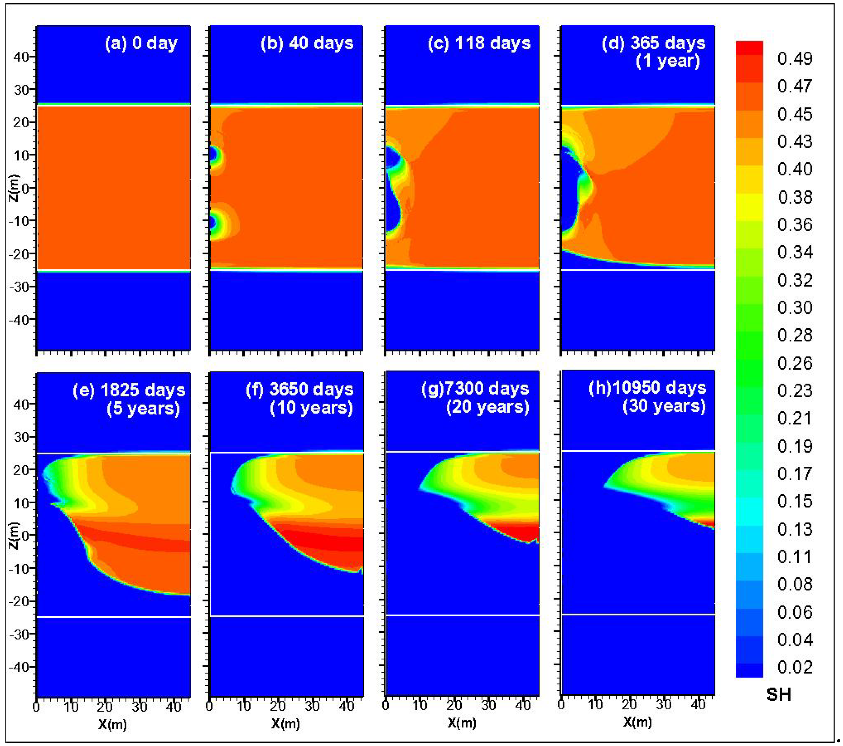
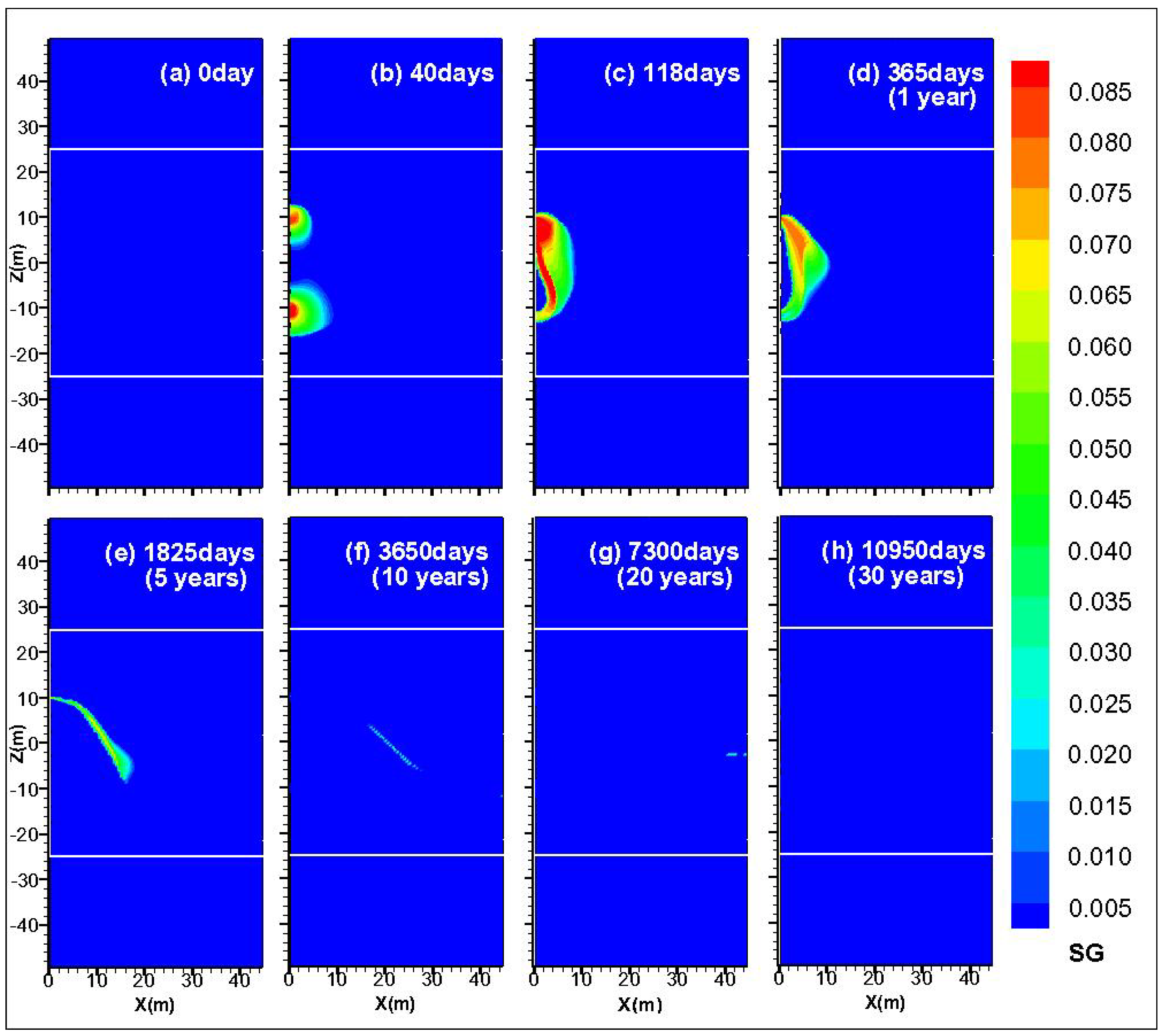
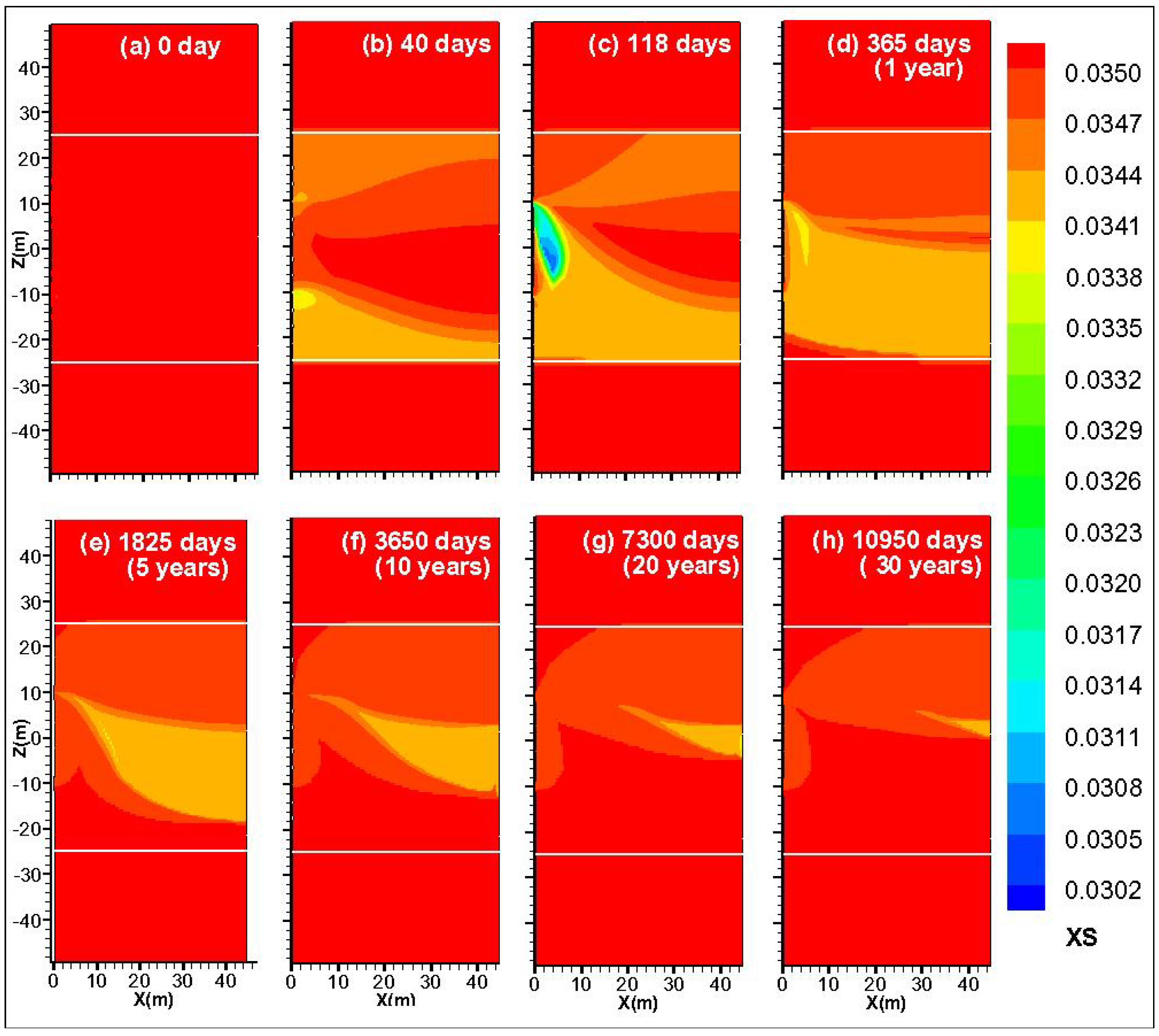
4.4. Spatial Distribution of S_H, S_G and X_S

Figure 6 and Figure 7 display the evolution of S_H (hydrate saturation) distributions and S_G (gas saturation) distributions during hydrate dissociation. It is shown from Figure 6 and Figure 7 that (i) during the initial 40 days, the hydrate is dissociated around the wells with limited cylindrical dissociation interfaces, and then the dissociation interfaces move forward (Figure 6b,c); (ii) the hydrate distribution region around the lower well is dissociated faster than that of the upper one (Figure 6c); (iii) after one year production, the hydrate located between the two wells is dissociated completely (Figure 6d); (iv) a dissociation interface emerges between the HBL and the underburden, and gradually merges with the cylindrical dissociation interface around the lower well (Figure 6d,e); (v) a similar dissociation interface occurs between the HBL and the overburden at about the 5th year (Figure 6e); (vi) limited secondary hydrate is formed in the front edge of the dissociation interface near the upper well in the initial 5 years, subsequently, some hydrate formed in the lower region of the hydrate reservoir (Figure 6b–h); (vii) the released gas accumulated around the frontier of the cylindrical dissociation interface (Figure 7b–e); (viii) the released gas nearly disappear after ten years exploitation (Figure 7f).

Figure 6. Evolution of the spatial distribution of S_H during hydrate dissociation (the Reference Case).

Figure 6. Evolution of the spatial distribution of S_H during hydrate dissociation (the Reference Case).

Of those, (i) and (iii) are the results of hydrate dissociation under the synergetic effect of depressurization, thermal stimulation, and inhibitor stimulation; (ii), (iv), and (v) are because on the one hand, the warm brine acts on the dissociation of hydrate located in the vicinity of the lower well, and on the other hand, the hydrate dissociation is influenced by the fluid flow from the overburden and the underburden; (vi) is because that the endothermic effect of hydrate dissociation causes the decrease of temperature near the dissociation interface, meanwhile, the released gas accumulates around this region, where the pressure condition is favorable for hydrate formation.

Figure 7. Evolution of the spatial distribution of S_G during hydrate dissociation (the Reference Case).

Figure 7. Evolution of the spatial distribution of S_G during hydrate dissociation (the Reference Case).

The secondary hydrate formation could reduce the effective permeability k_eff and prevent the released gas rising. (vii) and (viii) are because that the released gas is pumped out from the upper well as the dissociation interface enlarges. The hydrate between the two wells is dissociated completely after about 118 days. A channel connects the two wells as the dissociation interface expands. And then the injected warm brine tends to be produced from the upper well directly, which further results in the gas accumulation in the vicinity of the upper well. The interspace between the two wells weakens the heat conduction to the inner part of the HBL, and decreases the rate of gas releasing.

Figure 8 shows the evolution of the distributions of salt concentration X_S (the mass fraction of salt X_S in the aqueous phase) in the entire hydrate reservoir. As shown in Figure 8, X_S decrease in the hydrate dissociation area in the initial 40 days, which is due to the dilution effect of the free water released from the hydrate. As the injection process starts, the saline water from the overburden and underburden (both of them are permeable boundary) penetrates into the HBL under the effect of the depressurization, causing the increase of the higher X_S region. The X_S distribution in the vicinity of the wells on one hand increases with the influence of the injected brine, on the other hand decreases under the effect of the dilution.

Figure 8. Evolution of the spatial distribution of X_S during hydrate dissociation (the Reference Case).

Figure 8. Evolution of the spatial distribution of X_S during hydrate dissociation (the Reference Case).

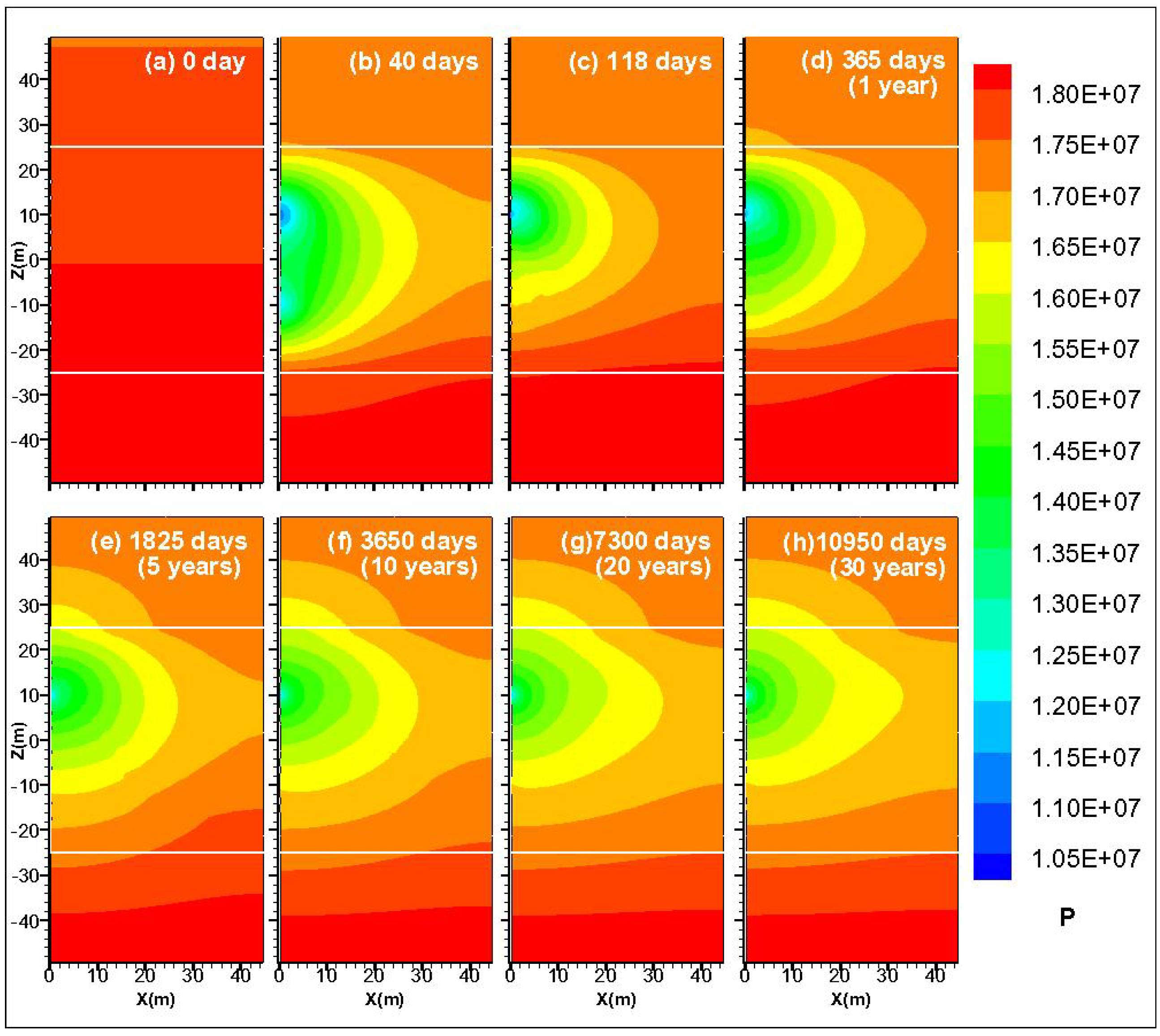
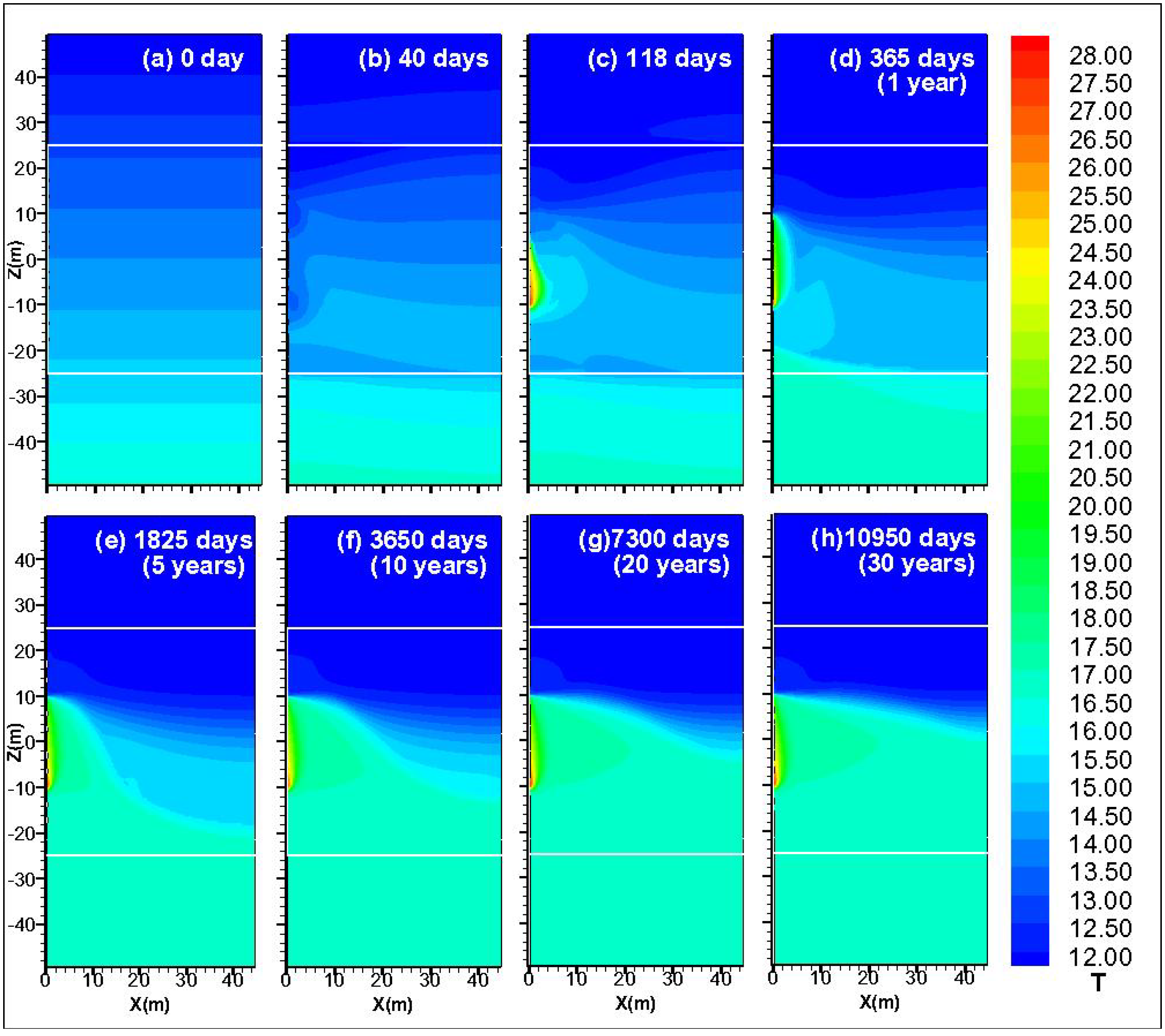
4.5. Spatial Distribution of P and T

Figure 9 shows the change of the pressure distributions over time in the whole hydrate deposit. The area between the white lines stands for the HBL. As can be seen in Figure 9, (i) there is a cylindrical pressure gradient around the well in the initial 40 days (Figure 9b); (ii) the depressurization trend moves up over time (Figure 9b–h); (iii) the pressure gradient decreases gradually (Figure 9b–h); (iv) the pressure distribution in the hydrate reservoir changes slowly from the 5th year to the 30th year (Figure 9e–h); (v) there are inflection points of pressure distribution on the white line between the overburden and the HBL (Figure 9d–h). Of those, (i) results from the simultaneous depressurization in the two wells; (ii) and (iii) are caused by the flow of the released fluid and the permeability of the boundary; (iv) is because that the gas-liquid flow field is relatively stable after the production well and injection well are connected; (v) originates from the different effective permeabilities of the overburden and the HBL.

Figure 10 demonstrates the evolution of the temperature distributions in the entire hydrate reservoir. As shown in Figure 10: (i) the temperature around the wells decreases because of the endothermic effect of hydrate dissociation (Figure 10b); (ii) the temperature declines near the top boundary of the HBL, and increases near the bottom boundary caused by the effect of fluids flow (Figure 10b); (iii) as the injection process starts, the temperature around the lower well increases and the heat is transferred deep into the HBL under the effect of the temperature gradient(Figure 10c–h); (iv) as soon as the hydrate between the two wells is dissociated completely, the temperature near the upper well rises because the injected warm brine flows up (Figure 10d–h); (v) the thermal gradient spreads further into the HBL over time due to the effect of fluids flow(Figure 10d–h); (vi) the temperature distribution in the whole hydrate reservoir changes slowly from 5 to 30 years because the fluid flow situation keeps stable during this period (Figure 10e–h). It is evident from Figure 10c–h that the temperature distributions in the overburden and underburden nearly keep unchangeable, which is attributed to that abundant saline water flow from the overburden and underburden to the initial HBL area.

Figure 9. Evolution of the spatial distribution of P during hydrate dissociation (the Reference Case).

Figure 9. Evolution of the spatial distribution of P during hydrate dissociation (the Reference Case).

Figure 10. Evolution of the spatial distribution of T during hydrate dissociation (the Reference Case).

Figure 10. Evolution of the spatial distribution of T during hydrate dissociation (the Reference Case).

4.6. Sensitivity Analyses

In this work, different cases are implemented to investigate the sensitivities of gas production on the temperature of the injected brine T_W, the salinity of the injected brine, and the intrinsic permeability k of the hydrate reservoir.

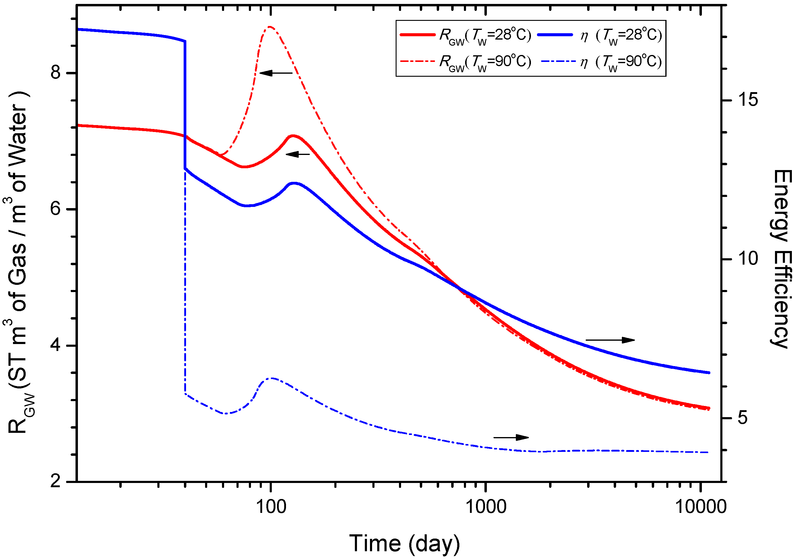
4.6.1. Sensitivity to the Temperature of the Injected Water T_W

Figure 11 shows the evolution of Q_PT, Q_R, and Q_W over time with different temperatures of the injected brine (T_W = 28 °C, 90 °C). In the reference case, T_W is 28 °C. The rest parameters between these two cases are same.

Figure 11. Evolution of Q_PT, Q_R, Q_W, and their dependence on the temperature of the injected brine during hydrate dissociation.

Figure 11. Evolution of Q_PT, Q_R, Q_W, and their dependence on the temperature of the injected brine during hydrate dissociation.

When T_W increases from 28 °C to 90 °C, it costs just 42 days (accounts for 35% of the reference case) to dissociate the hydrate blocking the region between the two wells. The peak value of Q_PT is 142.12 ST m³/day/m of well when T_W is 90 °C, which is 2.02 times larger than that of the reference case. The warm brine flows to the production well directly after the two wells are connected which diminishing the impact of heat convection and conduction. Thus, at the later stage of exploitation, the distinction of hydrate dissociation and gas production is mild between the two different T_W cases. Q_W increases with the enhancement of T_W as well. This is because more hydrate is dissociated under the stimulation of high temperature brine.

Figure 12 displays the dependence of R_GW and η on T_W. R_GW grows corresponding to the rise of Q_PT in the higher T_W case, which is because increasing the temperature of the injected brine can strengthen the heat-transfer effect. This phenomenon further results in advantageous gas production rate.

Figure 12. Evolution of the energy efficiency η, the gas-to-water ratio R_GW, and their dependence on the temperature of the injected brine during hydrate dissociation.

Figure 12. Evolution of the energy efficiency η, the gas-to-water ratio R_GW, and their dependence on the temperature of the injected brine during hydrate dissociation.

Unfortunately, the other criterion η declines remarkably with the enhancement of T_W, which is uneconomical for hydrate exploitation. This is because the higher T_W case needs more energy to heat the injected brine and causes more energy loss in the cause of injecting the brine.

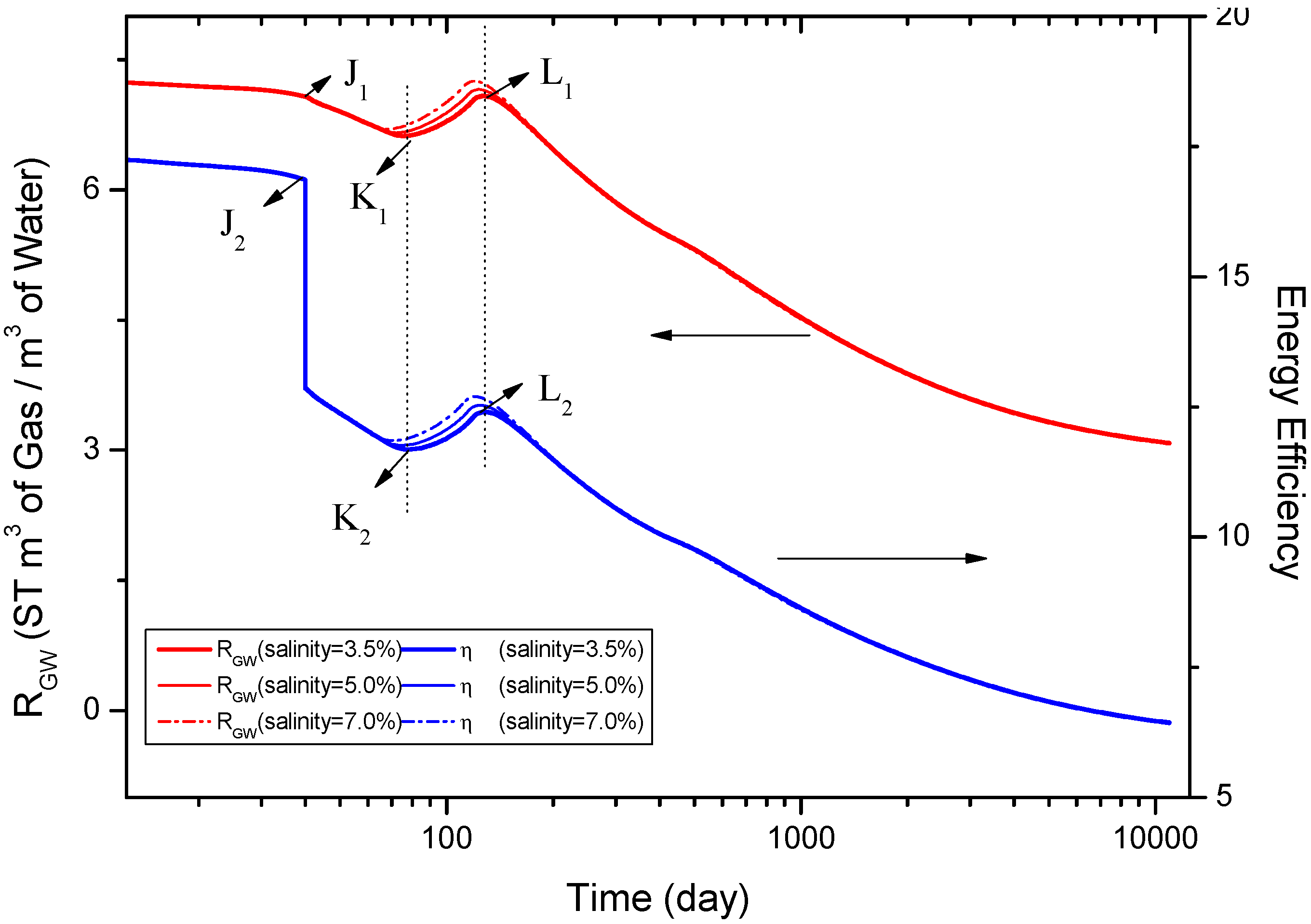
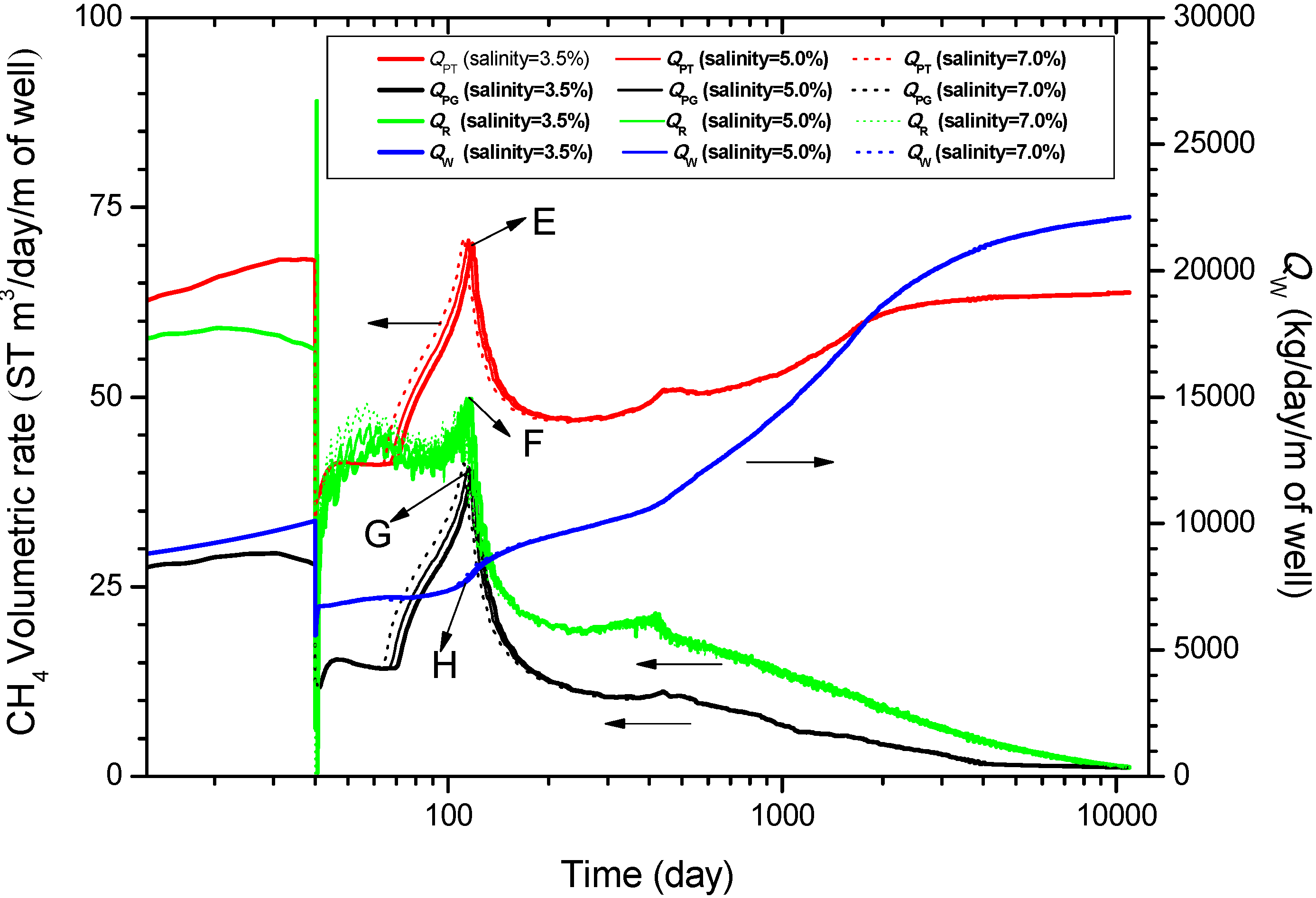
4.6.2. Sensitivity to the Salinity of the Injected Water

Figure 4 and Figure 5 show the evolution of Q_PT, Q_R, Q_W, R_GW, η, and their dependence on the salinity of the injected brine, respectively. In the reference case, the salinity of the injected brine is 3.5%. Except for the different salinity of the injected brine, the other system conditions in the three cases remained the same.

As shown in Figure 4, the profiles of Q_PT, Q_R, and Q_W from different cases are similar in the whole simulation process. The differences among the three cases appear as the injection process starts. Figure 4 shows that the higher the salinity of the injected brine is, the faster the Q_PT and Q_R become, which is in good agreement with the experimental investigation by Li et al. [10].

The model of the inhibitor effects on hydrate equilibrium can be simplified by the following equation [29]:

$$\mathrm{\Delta }{T}_D=\mathrm{\Delta }{T}_{D,r}\frac{\text{ln}(1-x_A^i)}{\text{ln}(1-x_{A,r}^i)}$$

(2)

Where $x_A^i$ is the mole fraction of the inhibitor in the aqueous phase; $x_{A,r}^i$ is the reference mole fraction of the inhibitor in the aqueous phase [K]; $\mathrm{\Delta }{T}_D$ is the inhibitor-induced temperature depression [K]; $\mathrm{\Delta }{T}_{D,r}$ is the temperature depression at the reference mole fraction $x_{A,r}^i$ As can be seen from Equation (2), when th $x_A^i$ (the salinity of the injected water) gets larger, it is more easily to break the hydrate equilibrium.

Once the hydrate blocking area between the two wells is dissociated completely, the distinction among the three cases gets smaller and almost fades away after 205 days injection. This is because that the injected warm brine can be pumped out through the cavity between the two wells to the upper production well directly, which weakens the inhibitor effects on the hydrate far from the injected well.

The injection rates of the brine are the same and the distinction of hydrate dissociation rates is little among the three cases. Thus the difference in Q_W is very small when the salinity of the injected brine increases from 3.5% to 7.0%. As shown in Figure 5, the gas-to-water ratio and the energy efficiency can be enhanced by increasing the salinity of the injected brine before the two horizontal wells are connected. Subsequently, the value of Q_W and η among the three cases almost keep the same, which is in line with the changes of gas and water production.

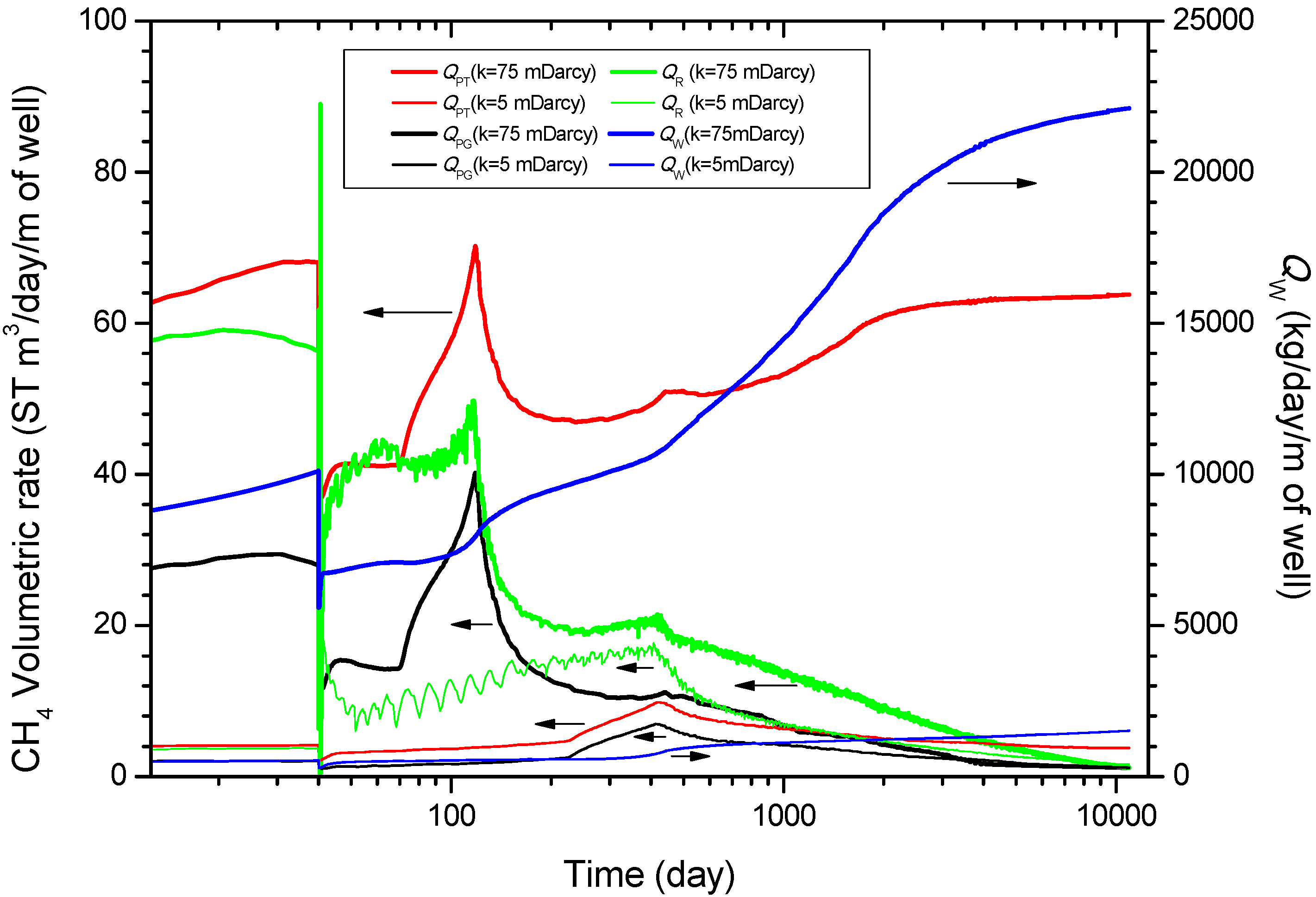
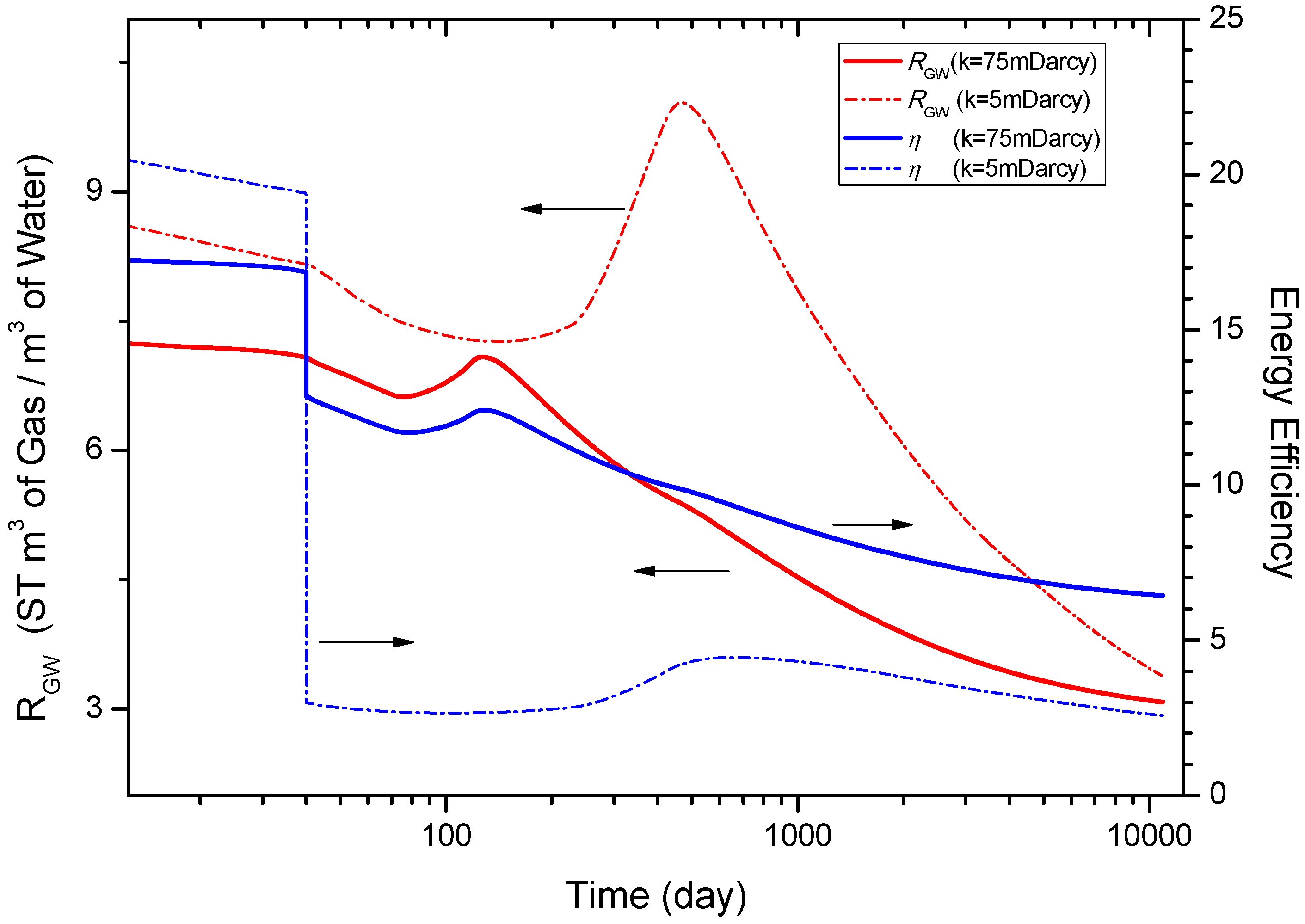
4.6.3. Sensitivity to the Intrinsic Permeability k of the Hydrate Reservoir

The effect of different intrinsic permeabilities of the hydrate reservoir on the production performance is also investigated. Except for the different intrinsic permeabilities of the two cases, the other operation conditions remain the same.

Figure 13 and Figure 14 show the dependences of Q_PT, Q_R, Q_W, R_GW, and η on the intrinsic permeability k of the hydrate reservoir, respectively. Reducing k from 75 mD to 5 mD causes a dramatic decline of gas production. Q_PT reaches the maximum value (70.19 ST m³/day/m of well) when the two wells are totally connected in the reference case. However, the maximum value of Q_PT is just 9.86 ST m³/day/m of well when k drops to 5 mD. In the later stage of simulation, Q_PT of the reference case is about 16.7 times larger than that of the lower k case. Moreover, the water production rate in the lower k case drops dramatically compared with the reference case. This is because when the intrinsic permeabilities become small, it’s more difficult for the fluids flow in the hydrate reservoir, which further decreases the production rate of gas/water.

Figure 13. Evolution of Q_PT, Q_R, Q_W, and their dependence on the intrinsic permeability k of the hydrate reservoir during hydrate dissociation.

Figure 13. Evolution of Q_PT, Q_R, Q_W, and their dependence on the intrinsic permeability k of the hydrate reservoir during hydrate dissociation.

Figure 14. Evolution of the energy efficiency η, the gas-to-water ratio R_GW, and their dependence on the intrinsic permeability k of the hydrate reservoir during hydrate dissociation.

Figure 14. Evolution of the energy efficiency η, the gas-to-water ratio R_GW, and their dependence on the intrinsic permeability k of the hydrate reservoir during hydrate dissociation.

Another noteworthy phenomenon is that Q_R is larger than Q_PT in the initial 1438 days. It means the produced gas mainly originates from the released gas from the hydrate reservoir rather than the gas dissolved in the produced water in the lower k case.

As shown in Figure 14, because of the substantial reduction of water production rate, R_GW in the lower k case is evidently larger than that in the reference case. The other criterion η is much lower than that of the reference case, which is uneconomic for gas production.

5. Conclusions

Based on the available limited data about the South China Sea, a marine hydrate reservoir model is established in order to investigate the gas production performance under warm brine stimulation combined depressurization with dual horizontal wells. The following conclusions can be drawn:

(1)

A dual horizontal well layout has been considered as the well configuration for this work. During the exploitation process, the upper well is regarded as the production well. A constant flow rate of warm brine is simultaneously injected into the hydrate reservoir through the lower well. For avoiding the pressure of the area around the lower well increase to an extremely high level by continuous injection at the start of the production process, a period of constant-pressure production in the lower well to decompose the hydrate and free the pores around the well is needed.

(2)

During the depressurization production stage, two cylindrical dissociation fronts exist around the two wells. As the injection process starts, the dissociation fronts enlarge with the injection of warm brine. The gas production rate increases when the hydrate between the two wells is gradually dissociated. Meanwhile, Q_PT and Q_R reach the peak value when the two wells are connected completely. A dissociation interface emerges between the HBL and the underburden, and then gradually merges with the cylindrical dissociation interface around the lower well. A similar dissociation interface occurs in the upper well and the overburden lately.

(3)

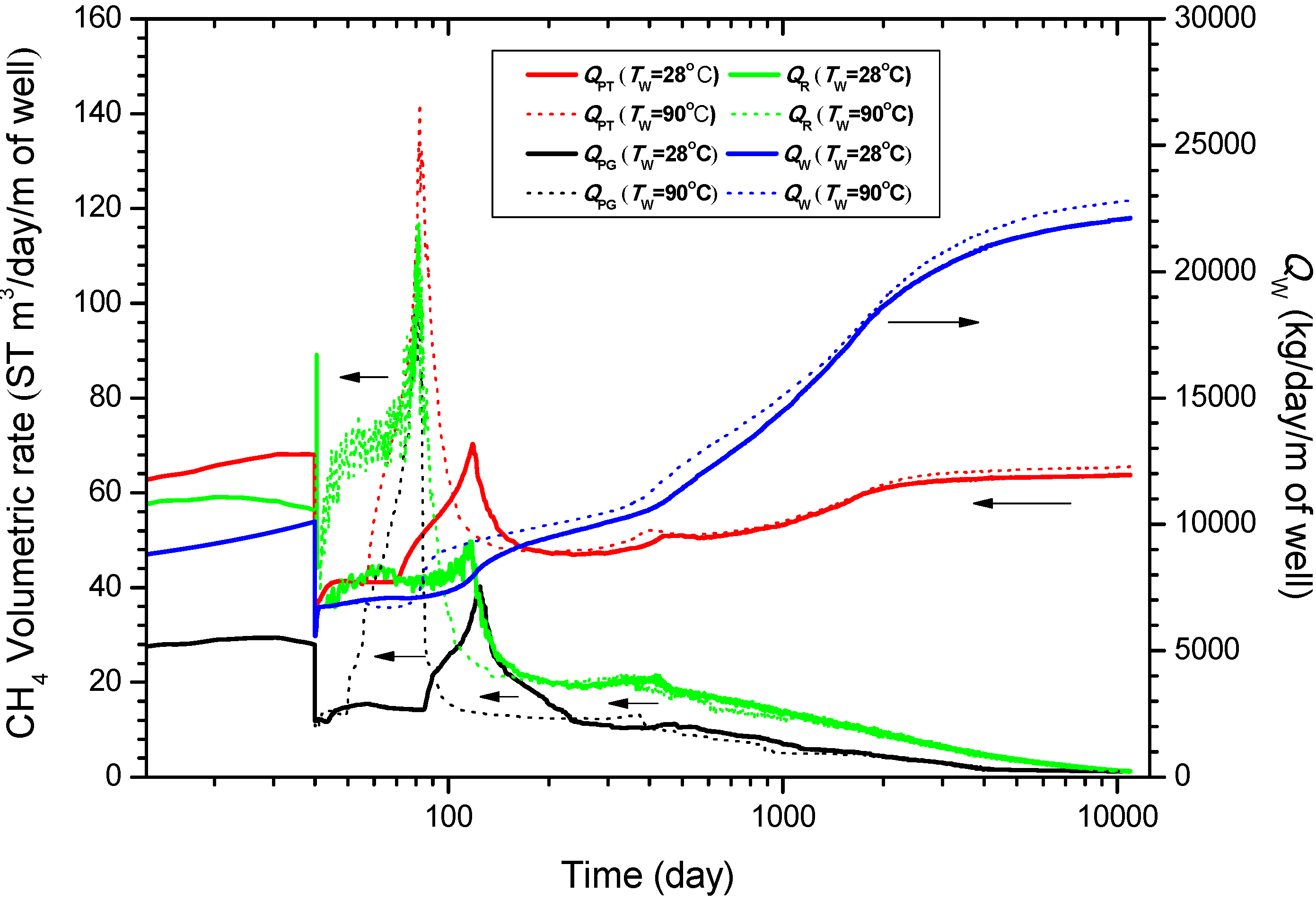
In the reference case, Q_PT exceeds Q_R and Q_PG in the whole production of 30 years, indicating that most of the produced gas comes from the CH₄ dissolved in the water rather than from the free gas. A maximum value (17.3 ST m³/day/m) of Q_PT is obtained before a decline starts at the 118th day. The variation of Q_R is similar to that of Q_PT. The average gas production rate Q_avg is about 1.23 × 10⁵ ST m³/day for a 1000 m-long well with spacing of 90 m, which can obtain the same order of magnitude compared with the commercially viable production rate. The corresponding water production rate Q_W is about 3.98 × 10⁷ kg/day which is massive. Furthermore, it causes a relative low level of R_GW (from 3.08 to 7.35). The other criterion η gets the range of 6.43 to 17.5. The simulation results provide economical feasibility of the warm brine stimulation combined depressurization method from the point of high level of energy efficiency.

(4)

The analysis of sensitivity to the temperature of the injected brine indicates that increasing T_W can enhance Q_PT, Q_R, and R_GW remarkably when the injection process starts. However, the advantage gradually disappears as the hydrate blocking the channel of the two wells is dissociated totally. The analysis of sensitivity to the salinity of the injected brine comes to the conclusion that the larger the X_S is, the faster the gas production rate is. But this advantage gradually fades away after the two wells are connected. Consequently, some practical methods such as enlarging the distance between the two wells may be taken into account to make the warm brine injected deep into the hydrate reservoir.

(5)

Sensitivity analysis shows that the gas and water production are strongly dependent on the intrinsic permeability of the hydrate reservoir. The gas and water production rates decrease when the intrinsic permeability decline from 75 mD to 5 mD. The energy efficiency η also gets an evident decrease with the reduction of k, on the other hand, an obvious enhancement of the gas-to-water ratio R_GW can be observed. When k decreases to 5 mD, Q_R is larger than Q_PT in the initial 1475 days, suggesting that the produced gas mainly comes from the released gas.

References

1. Shiraki, M. Physical characterization of TRK-720 hydrate, the very late Antigen-4 (VLA-4) inhibitor, as a solid form for inhalation: Preparation of the hydrate by solvent exchange among its solvates and mechanistical considerations. J. Pharm. Sci. 2010, 99, 3986–4004. [Google Scholar] [PubMed]
2. Sloan, E.D.; Koh, C.A. Clathrate Hydrates of Natural Gases, 3rd ed.; CRC Press: Boca Raton, FL, USA, 2008. [Google Scholar]
3. Moridis, G.J. Challenges, uncertainties and issues facing gas production from gas hydrate deposits. SPE Reserv. Eval. Eng. 2011, 14, 76–112. [Google Scholar] [CrossRef]
4. Li, G.; Li, B.; Li, X.S.; Zhang, Y.; Wang, Y. Experimental and numerical studies on gas production from methane hydrate in porous media by depressurization in pilot-scale hydrate simulator. Energy Fuels 2012, 26, 6300–6310. [Google Scholar] [CrossRef]
5. Zhao, J.F.; Yu, T.; Song, Y.C.; Liu, D.; Liu, W.G.; Liu, Y.; Yang, M.J.; Ruan, X.K.; Li, Y.H. Numerical simulation of gas production from hydrate deposits using a single vertical well by depressurization in the Qilian Mountain permafrost, Qinghai-Tibet Plateau, China. Energy 2013, 52, 308–319. [Google Scholar] [CrossRef]
6. Li, X.S.; Wang, Y.; Duan, L.P.; Li, G.; Zhang, Y.; Huang, N.S.; Chen, D.F. Experimental investigation into methane hydrate production during three-dimensional thermal huff and puff. Appl. Energy 2012, 94, 48–57. [Google Scholar] [CrossRef]
7. Mohammadi, A.H.; Richon, D. Phase equilibria of hydrogen sulfide and carbon dioxide simple hydrates in the presence of methanol, (methanol plus NaCl) and (ethylene glycol plus NaCl) aqueous solutions. J. Chem. Thermodyn. 2012, 44, 26–30. [Google Scholar] [CrossRef]
8. Moridis, G.J.; Collett, T.S.; Dallimore, S.R.; Satoh, T.; Hancock, S.; Weatherill, B. Numerical studies of gas production from several CH4 hydrate zones at the Mallik site, Mackenzie Delta, Canada. J. Petrol. Sci. Eng. 2004, 43, 219–238. [Google Scholar] [CrossRef]
9. Li, G.; Tang, L.; Huang, C.; Feng, Z.; Fan, S. Thermodynamic evaluation of hot brine stimulation for natural gas hydrate dissociation. J. Chem. Ind. Eng. (China) 2006, 57, 2033–2038. [Google Scholar]
10. Li, X.S.; Wan, L.H.; Li, G.; Li, Q.P.; Chen, Z.Y.; Yan, K.F. Experimental investigation into the production behavior of methane hydrate in porous sediment with hot brine stimulation. Ind. Eng. Chem. Res. 2008, 47, 9696–9702. [Google Scholar] [CrossRef]
11. Moridis, G.J.; Reagan, M.T.; Boyle, K.L.; Zhang, K. Evaluation of the gas production potential of some particularly challenging types of oceanic hydrate deposits. Transp. Porous Media 2011, 90, 269–299. [Google Scholar] [CrossRef]
12. Moridis, G.J.; Collett, T.S.; Boswell, R.; Kurihara, M.; Reagan, M.T.; Koh, C.; Sloan, E.D. Toward production from gas hydrates: current status, assessment of resources, and simulation-based evaluation of technology and potential. SPE Reserv. Eval. Eng. 2009, 12, 745–771. [Google Scholar] [CrossRef]
13. Japan Taps “Fiery Ice” Fuel from Seabed. Available online: http://www.newscientist.com/blogs/shortsharpscience/2013/03/japan-taps-methane-hydrate-fro.html (accessed on 13 March 2013).
14. Boswell, R.; Frye, M.; Shelander, D.; Shedd, W.; McConnelle, D.R.; Cook, A. Architecture of gas-hydrate-bearing sands from Walker Ridge 313, Green Canyon 955, and Alaminos Canyon 21: Northern deepwater Gulf of Mexico. Mar. Pet. Geol. 2012, 34, 134–149. [Google Scholar] [CrossRef]
15. Myshakin, E.M.; Gaddipati, M.; Rose, K.; Anderson, B.J. Numerical simulations of depressurization-induced gas production from gas hydrate reservoirs at the Walker Ridge 313 site, northern Gulf of Mexico. Mar. Petrol. Geol. 2012, 34, 169–185. [Google Scholar] [CrossRef]
16. Trung, N.N. The gas hydrate potential in the South China Sea. J. Petrol. Sci. Eng. 2012, 88–89, 41–47. [Google Scholar]
17. Liu, H.L.; Yao, Y.J.; Deng, H. Geological and geophysical conditions for potential natural gas hydrate resources in southern South China Sea waters. J. Earth Sci. (China) 2011, 22, 718–725. [Google Scholar] [CrossRef]
18. Wang, C.J.; Du, D.W.; Zhu, Z.W.; Liu, Y.G.; Yan, S.J.; Yang, G. Estimation of potential distribution of gas hydrate in the northern South China Sea. Chin. J. Oceanol. Limn. 2010, 28, 693–699. [Google Scholar] [CrossRef]
19. Li, G.; Moridis, G.J.; Zhang, K.; Li, X.S. The use of huff and puff method in a single horizontal well in gas production from marine gas hydrate deposits in the Shenhu Area of South China Sea. J. Petrol Sci. Eng. 2011, 77, 49–68. [Google Scholar] [CrossRef]
20. Su, Z.; Moridis, G.J.; Zhang, K.; Wu, N. A huff-and-puff production of gas hydrate deposits in Shenhu area of South China Sea through a vertical well. J. Petrol. Sci. Eng. 2012, 86–87, 54–61. [Google Scholar]
21. Yao, B.C. The gas hydrate in the South China Sea. J. Trop. Oceanogr. 2001, 20, 20–28. [Google Scholar]
22. Wang, S.; Yan, W.; Song, H. Mapping the thickness of the gas hydrate stability zone in the South China Sea. Terr. Atmos. Ocean Sci. 2006, 17, 815–828. [Google Scholar]
23. Moridis, G.J.; Reagan, M.T. Strategies for Gas Production From Oceanic Class 3 Hydrate Accumulations. In Proceedings of the OTC 18865, 2007 Offshore Technology Conference, Houston, TX, USA, 30 April–3 May 2007.
24. Moridis, G.J.; Reagan, M.T.; Boyle, K.L.; Zhang, K. Evaluation of the Gas Production Potential of Challenging Hydrate Deposits. In TOUGH Symposium; Lawrence Berkeley National Laboratory: Berkeley, CA, USA, 14–16 September 2009. [Google Scholar]
25. Li, X.S.; Zhang, Y.; Li, G.; Chen, Z.Y.; Wu, H.J. Experimental investigation into the production behavior of methane hydrate in porous sediment by depressurization with a novel three-dimensional cubic hydrate simulator. Energy Fuels 2011, 25, 4497–4505. [Google Scholar] [CrossRef]
26. Konno, Y.; Masuda, Y.; Hariguchi, Y.; Kurihara, M.; Ouchi, H. Key factors for depressurization-induced gas production from oceanic methane hydrates. Energy Fuels 2010, 24, 1736–1744. [Google Scholar] [CrossRef]
27. Moridis, G.J.; Reagan, M.T.; Zhang, K. The Use of Horizontal Wells in Gas Production from Hydrate Accumulations. In Proceedings of the 6th International Conference on Gas Hydrates (ICGH 2008), Vancouver, BC, Canada, 6–10 July 2008.
28. Li, X.S.; Li, B.; Li, G.; Yang, B. Numerical simulation of gas production potential from permafrost hydrate deposits by huff and puff method in a single horizontal well in Qilian Mountain, Qinghai province. Energy 2012, 40, 59–75. [Google Scholar] [CrossRef]
29. Moridis, G.J.; Kowalsky, M.B.; Pruess, K. Tough+Hydrate v1.1 User’s Manual: A Code for the Simulation of System Behavior in Hydrate-Bearing Geologic Media; Lawrence Berkeley National laboratory: Berkeley, CA, USA, 2009. [Google Scholar]
30. Wang, D.; Li, D.L.; Zhang, H.L.; Fan, S.S.; Zhao, H.B. Laboratory measurement of longitudinal wave velocity of artificial gas hydrate under different temperatures and pressures. Sci. China Ser. G Phy. Mech. Astron. 2008, 51, 1905–1913. [Google Scholar] [CrossRef]
31. Gamwo, I.K.; Liu, Y. Mathematical modeling and numerical simulation of methane production in a hydrate reservoir. Ind. Eng. Chem. Res. 2010, 49, 5231–5245. [Google Scholar] [CrossRef]
32. Liu, Y.; Strumendo, M.; Arastoopour, H. Simulation of methane production from hydrates by depressurization and thermal stimulation. Ind. Eng. Chem. Res. 2009, 48, 2451–2464. [Google Scholar] [CrossRef]
33. Yao, B.C.; Yang, M.Y.; Wu, S.G.; Wang, H.B. The gas hydrate resources in the China seas. Geoscience (China) 2008, 22, 333–341. [Google Scholar]
34. Van Genuchten, M.T. A closed-form equation for predicting the hydraulic conductivity of unsaturated soils. Soil Sci. Soc. Am. J. 1980, 44, 892–898. [Google Scholar] [CrossRef]
35. Moridis, G.J.; Seol, Y.; Kneafsey, T.J. Studies of Reaction Kinetics of Methane Hydrate Dissociation in Porous Media. In Proceedings of the 5th International Conference on Gas Hydrate, Trondheim, Norway, 3–5 June 2005; pp. 1004–1014.