Analysis of Power System Cost Evolution Characteristics Under Different Thermal Power Substitution Modes

Abstract

With the continuous decline in the cost of renewable energy such as wind power and photovoltaic power generation, the economic competitiveness in the power supply structure is increasing, and traditional thermal power units are gradually being replaced, resulting in a profound adjustment of the power supply structure. However, the unclear alternative between units may lead to system redundancy configuration or power supply shortage. At the same time, the volatility of the new energy output and the flexible allocation of resources and other factors work together, resulting in the cost of the power system showing complex evolution characteristics. Therefore, it is of great significance to study the evolution of system cost in the process of thermal power substitution. This paper first analyzes the internal mechanism of the cost change of the new power system. Second, the cost accounting model of the power system is constructed to reveal the relationship between ‘thermal power substitution mode-system cost’ in the process of thermal power installed capacity substitution. Finally, the Garver-6 system is taken as an example to carry out simulation analysis, solve the optimal thermal power substitution mode under different renewable energy penetration rates, and explore the evolution law of system cost. The results of the example show that with the increase of renewable energy penetration, the total cost of the system first decreases and then increases, and the optimal substitution method is ‘unit thermal power to replace more renewable energy’.

1. Introduction

In the development stage of the traditional power system, the power structure is dominated by fossil fuel units. The power generation side exhibits strong controllability and stability, and the system operation follows the typical “generation follows load” scheduling logic, resulting in a relatively stable system cost structure [1,2]. Historically, provinces such as Shanxi, Shaanxi, Liaoning, Jilin, and Heilongjiang have had abundant coal reserves and a well-developed infrastructure, which were the primary prerequisites for the development of thermal power plants in Northeast and Central China. It is also worth noting that, historically, thermal power plants in China were developed using a condensing cycle. By the end of 2025, the installed capacity of renewable energy in China had exceeded 2.159 billion kW, accounting for 59.2% of the country’s total installed power generation capacity, surpassing thermal power for the first time to become the dominant power source in the power system [3]. The high penetration of wind and photovoltaic power has gradually shifted the power supply side from being predominantly controllable to predominantly stochastic. The volatility and uncertainty of the renewable energy output have been significantly enhanced, and the system operation logic has gradually evolved from “generation follows load” to a new paradigm of “source–load bidirectional interaction” and even “load follows generation” [4,5]. Meanwhile, the large-scale integration of new resources such as distributed generation and energy storage has progressively transformed the power system structure from a centralized network with traditional unidirectional power flow to a complex network system characterized by multi-node, multi-agent collaborative interaction [6,7]. This structural transformation of the new power system, by increasing the demand for flexibility resources and strengthening real-time balancing and coordination management, has shifted the system costs from being stable and controllable to being highly complex and heavily dependent on flexibility.

The above structural changes do not simply reduce the overall cost of the system but profoundly reshape the cost structure of the power system. On the one hand, renewable energy has a low marginal generation cost. As its installed capacity continues to expand, it has gradually become the dominant power source in the new power system. The share of fuel costs in the total cost of power generation is gradually decreasing [8], leading to a reduction in the cost of electricity production. However, the change in the system’s energy structure introduces power and energy balance issues. To cope with the power deviations caused by fluctuations in renewable energy output, the system’s demand for flexibility resources has increased significantly. This includes increased investments in energy storage power and capacity allocation, flexible retrofitting of thermal power plants, and the construction of peak-shaving and frequency-regulation resources. Reference [9] effectively alleviates the long-term supply–demand imbalance risk in the system by constructing a flexibility resource allocation mechanism for managing long-term supply–demand imbalance risks. Reference [10] constructs a source–storage–transmission joint planning model, improving the overall regulation capability of the system through energy storage participation. Reference [11] points out that when a sudden flexibility shortage occurs in the system, energy storage can achieve energy throughput and regulation compensation through emergency dispatch, thereby alleviating system operation risks. China’s national power grid currently has approximately 30 Ultra-High Voltage Direct Current (UHVDC) lines, which facilitate the integration of large-scale solar and wind power plants by enabling long-distance, low-loss transmission of renewable energy from resource-rich regions to load centers.

At the same time, the centralized development of wind and solar power, together with the need for large-scale long-distance transmission, has revealed insufficient grid strength in the existing system. Existing transmission corridors in some regions struggle to meet power transmission demands, making grid expansion and transmission capacity enhancement important supporting measures for renewable energy integration. References [12,13] avoid waste in energy storage investment and redundancy in line expansion by optimizing the coordinated planning of energy storage and transmission lines, effectively improving weak links in the grid. Based on a mixed-integer linear programming (MILP) approach, References [14,15,16] minimize transmission investment costs while ensuring line transmission capacity.

Therefore, compared with the traditional power system, the cost change in the new power system is a systematic reconstruction process driven jointly by the transformation of the power supply structure and the change in system operation mechanisms [17,18]. It is not merely a simple substitution of traditional energy sources (such as coal and natural gas) with higher marginal costs by renewable energy sources (such as wind and solar) with very low marginal costs. The shift in system operation mode caused by the change in system structure makes the calculation of system costs more complex. In this context, characterizing the evolution of system costs under different renewable energy penetration rates and revealing the impact of flexibility resource allocation on cost changes have become key issues in new power system research. However, existing research mostly focuses on the economic analysis of a single technology or static scenario comparisons, lacking a systematic characterization of the dynamic evolution path of overall system costs. Based on this, it is necessary to construct a multi-scenario, multi-agent collaborative analysis framework to systematically study the reconstruction process and evolution mechanism of the power system cost structure under high renewable energy penetration, thereby providing a decision-making basis for power structure optimization and system cost control under high renewable energy penetration.

To clarify the cost composition structure of the new power system, distinguish the cost shares of its various components (power sources and regulation resources), analyze the factors driving system cost changes, and thereby understand the evolution law of system costs during renewable energy development, this paper provides path guidance for power structure optimization and regulation resource allocation under the new power system. Specifically, this paper carries out the following:

(1)

Analyzes the factors driving system cost changes

(2)

Defines the substitution method between traditional thermal units and renewable energy

(3)

Constructs a cost accounting model for the power system

(4)

Uses the Garver-6 system as a case study to conduct simulation analysis, determine the optimal thermal power substitution mode under different renewable energy penetration rates, and explore the evolution law of system costs.

2. Analysis of System Cost Change Motivation

To clarify the evolution of system costs during increasing renewable energy penetration, it is first necessary to identify the factors influencing system costs. This section examines four key aspects: power system transformation, flexibility requirements under different renewable penetration scenarios, the impact of transmission lines on system flexibility and costs, and the determination of thermal power substitution modes. The objective is to clarify what factors affect system costs and how they evolve. A detailed point-by-point analysis is provided below.

2.1. Energy Structure Transformation

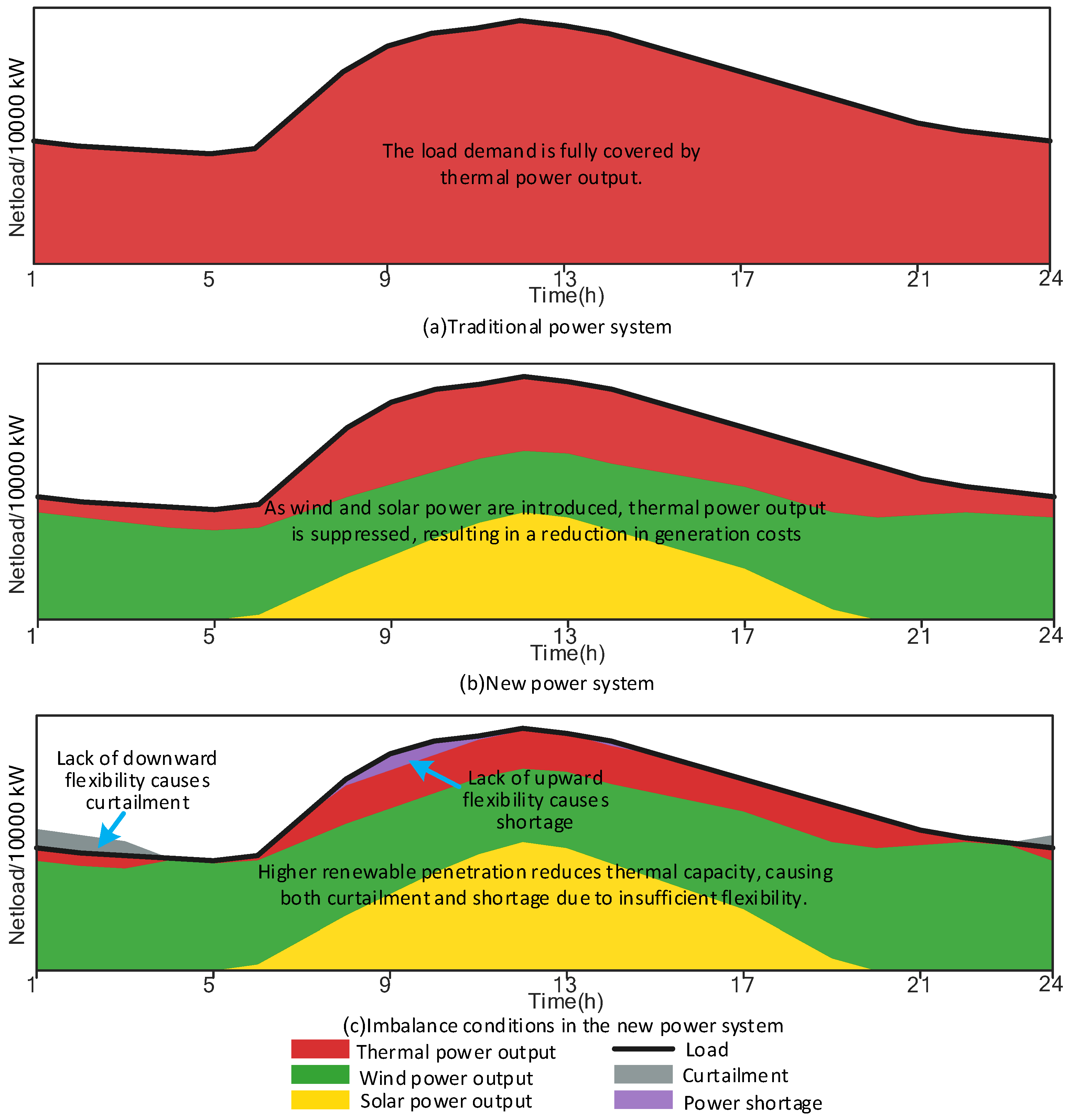
In the new power system, the “source” side, i.e., the electricity production stage, undertakes the core function of converting primary energy into electrical energy and connecting it to the power grid. As shown in Figure 1 (drawn by the authors), the profound transformation of the energy structure from traditional fossil fuels to high-proportion renewable energy is becoming one of the key driving factors behind system cost changes.

With the acceleration of the energy transition, the energy structure of the new power system is undergoing profound changes. The installed capacity of clean energy sources such as wind and solar power is increasing rapidly, gradually replacing traditional thermal power generation. However, wind and solar power are characterized by intermittency, volatility, and randomness, and cannot generate power on demand like traditional sources. Consequently, the power supply has shifted from being deterministic to uncertain. When renewable energy generation is high, it cannot be fully absorbed by the power grid, resulting in curtailment of wind and solar power. Conversely, during periods with no wind or sunlight, or during peak demand, power shortages occur. Thus, curtailment and shortage coexist.

To address these issues, the new power system requires more flexible resources, such as battery energy storage and pumped storage hydropower. The investment and operational costs of these resources are very high. As the share of renewable energy increases, the demand for such resources also grows, which significantly increases the overall system cost. The transformation from the traditional power system to the new power system is fundamentally a shift from a centralized dispatch mode dominated by controllable power sources to a multi-energy complementary mode with large-scale renewable energy integration. This transformation also changes the system’s operation mode and cost structure.

2.2. Flexibility Analysis of New Power System

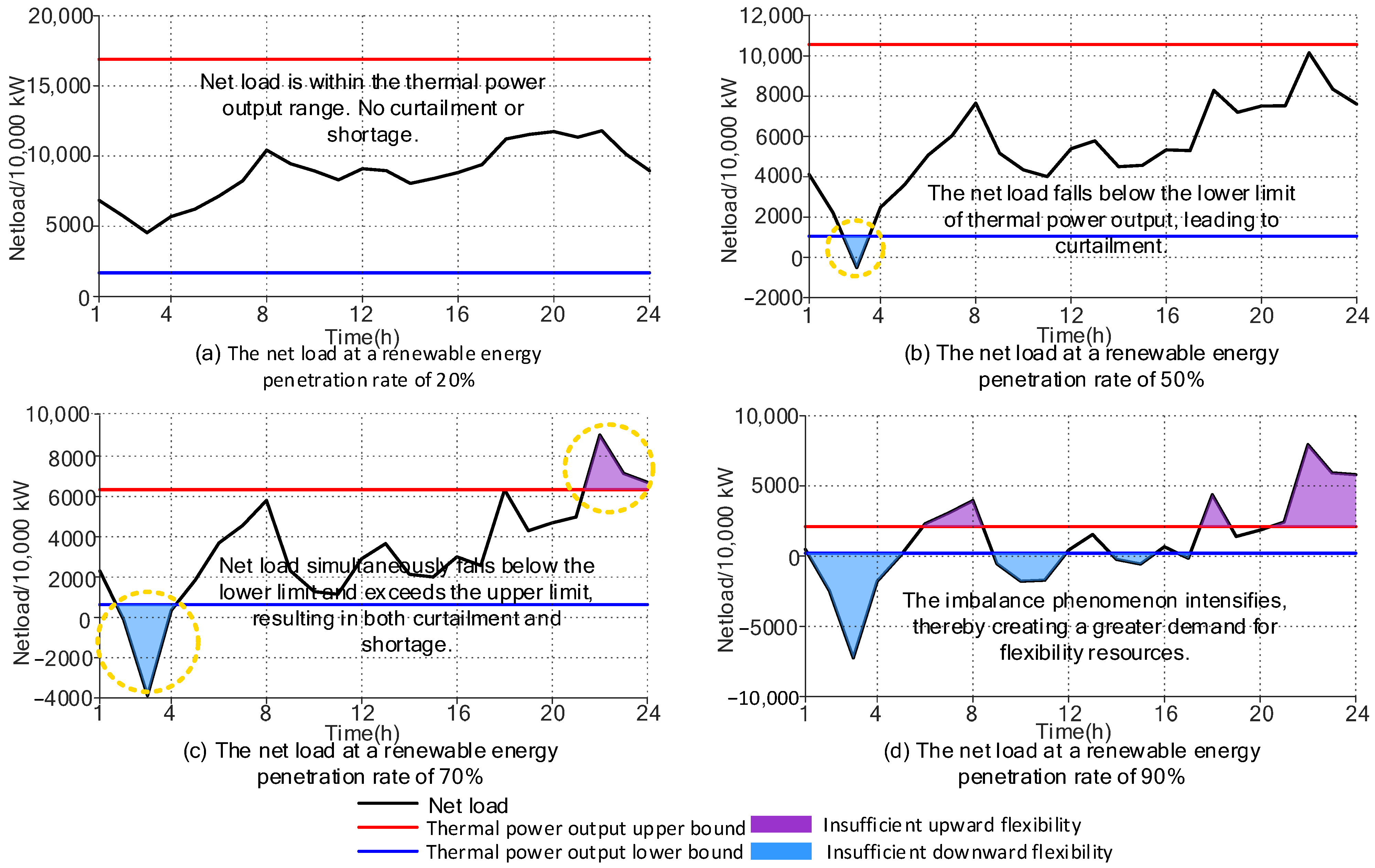
Under different renewable energy penetration rates, the net load curve exhibits significant variation, which in turn imposes differentiated requirements on the regulation capability of flexible resources. Taking a typical 24 h operating day of the new power system as an example, this study reveals the factors influencing system cost changes by comparing net load and curtailment characteristics across various penetration rates.

As shown in Figure 2, in the low penetration rate stage illustrated in Figure 2a, as the renewable energy penetration rate increases, thermal power remains the absolute main body, undertaking the base load and most of the flexibility tasks. At this stage, system flexibility is abundant, generation costs decrease, and the system cost shows a declining trend.

When the renewable energy penetration rate reaches 50%, as shown in Figure 2b, the net load becomes negative and falls below the thermal power output lower bound. At this point, relying solely on thermal power peak regulation can no longer meet system flexibility requirements, and curtailment occurs. Additional flexibility resources are needed to regulate the power balance, leading to an increase in system cost.

As the renewable energy penetration rate rises to 70% or even higher, as shown in Figure 2c,d, thermal power gradually transforms from a base load power source to a regulating power source, with some units being retired. During specific periods, such as hours 2–4, even when the thermal power output has been reduced to its minimum, the wind and solar output still exceed the load, resulting in mandatory curtailment. During hours 22–24, insufficient upward flexibility occurs, and part of the load cannot be supplied. The source–load temporal mismatch intensifies, and curtailment and shortage occur simultaneously within a single day. More flexibility resources need to be added to shift the power and reduce the occurrence of imbalance events, leading to a significant increase in system cost.

Through the analysis of the above four daily penetration rate scenarios, it can be seen that with the increase in renewable energy penetration, although clean, low-cost wind and solar power have replaced relatively expensive thermal power, the decline in thermal power installed capacity has led to a serious shortage of system flexibility. Flexibility resources must be allocated to address curtailment and shortage in the system. The resulting increase in regulation cost leads to a change in the total system cost.

2.3. Analysis of Line Expansion of New Power System

In the process of the transformation of the new power system, more and more new power sources such as distributed photovoltaic and distributed wind power are beginning to be connected to the transmission grid. This results in the traditional ‘centralized power generation, long-distance transmission’ model changing. The new model should not only achieve local balance but also achieve wide-area mutual assistance.

This change has also led to a strategic shift in the expansion of the transmission network. The focus of grid investment is changing. In the traditional power system, the investment is mainly focused on large thermal power and hydropower bases. However, the focus of investment in the new power system has shifted to areas with rich scenery resources but they may be far away from the power center. These areas are also known as new energy hubs. The extension and strengthening direction of transmission lines are densely directed to the collection stations of large-scale wind power and photovoltaic clusters. At the same time, in order to integrate the distributed power supply, it is also very important to strengthen the transmission channel and regional networking lines of the original distribution network.

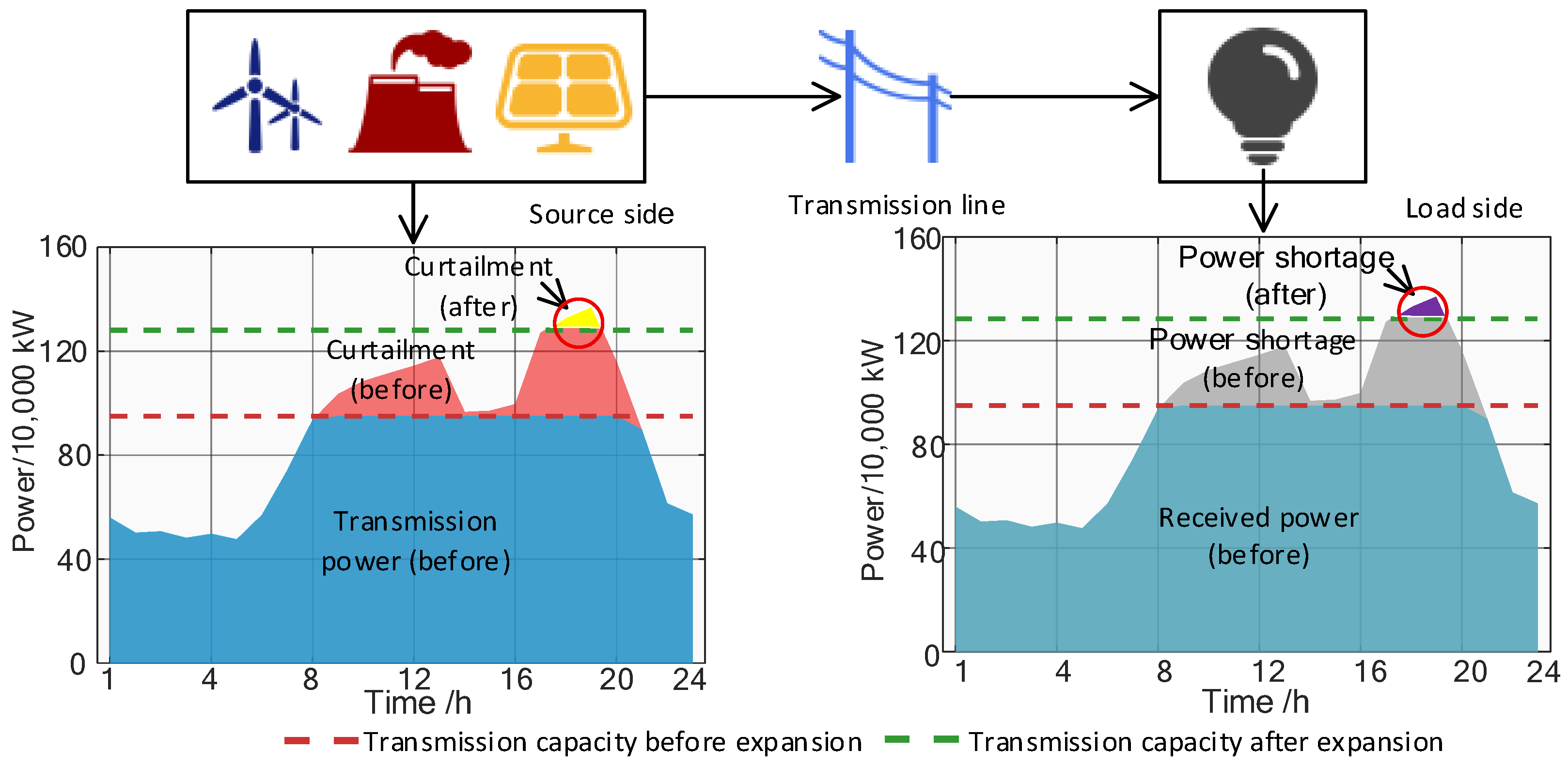
As shown in Figure 3, unlike thermal power with stable and controllable output, wind and solar power are characterized by intermittency and strong randomness. To ensure that all electricity can be transmitted and utilized during concentrated output periods, and to avoid curtailment caused by network congestion, line planning cannot be based solely on average transmission power. Instead, it is necessary to increase the number of line circuits and coordinate them with energy storage to ensure transmission capacity while reducing imbalances on both the source side and the load side. Consequently, system costs will change; increasing the number of transmission line circuits raises grid investment, while reducing imbalances caused by insufficient transmission capacity lowers system penalty costs.

2.4. Determination of the Thermal Power Substitution Mode

The replacement ratio of thermal power installed capacity is also a factor affecting system cost. If thermal power replaces less new energy, the phenomenon of power abandonment may occur; if more new energy is replaced, the load may not be supplied. In this paper, alternative mode 2 is set up: with the increase of the renewable energy penetration rate by 10%, the thermal power will reduce the load supply by 10%, so as to calculate the power generation capacity of the thermal power and calculate the installed capacity of the thermal power under different penetration rates with equivalent utilization hours of 4500 h. By analogy, the installed capacity of thermal power units under different alternative modes is obtained, as shown in

Table 1. Thermal power installed capacity under different penetration rates (Unit: 10,000 kW).

RE Penetration Rate	0%	10%	20%	30%	40%	50%	60%	70%	80%	90%	100%
Mode 1	2111	2111	2111	2111	2111	2111	2111	2111	2111	2111	2111
Mode 2	2111	2090	2069	2048	2027	2006	1985	1964	1942	1921	1900
Mode 3	2111	2069	2027	1985	1942	1900	1858	1816	1774	1731	1689
Mode 4	2111	2048	1985	1921	1858	1795	1731	1668	1605	1541	1478
Mode 5	2111	2027	1942	1858	1774	1689	1605	1520	1436	1351	1267
Mode 6	2111	2006	1900	1795	1689	1584	1478	1372	1267	1161	1056
Mode 7	2111	1985	1858	1731	1605	1478	1351	1225	1098	971	845
Mode 8	2111	1964	1816	1668	1520	1372	1225	1077	929	781	633
Mode 9	2111	1942	1774	1605	1436	1267	1098	929	760	591	422
Mode 10	2111	1921	1731	1541	1351	1161	971	781	591	401	211

.

3. Power System Cost Accounting Model and Cost Evolution

To characterize the evolution of power system costs under increasing renewable energy penetration, this chapter develops a comprehensive optimization model for power system cost accounting. The model is formulated within a Mixed Integer Linear Programming (MILP) framework to ensure computational tractability while accurately capturing the operational characteristics of thermal power units, renewable generation, and energy storage systems. This paper uses a DC power flow model. Therefore, the model considers only active power and voltage phase angles. All calculations are performed with a mandatory active power balance. Reactive power and voltage magnitude variations at nodes are not considered. This is a common simplification in power system expansion planning studies. This study adopts a deterministic modeling framework. Hourly wind and solar generation profiles, as well as load profiles, are treated as known exogenous inputs.

3.1. Power System Cost Accounting Model Framework

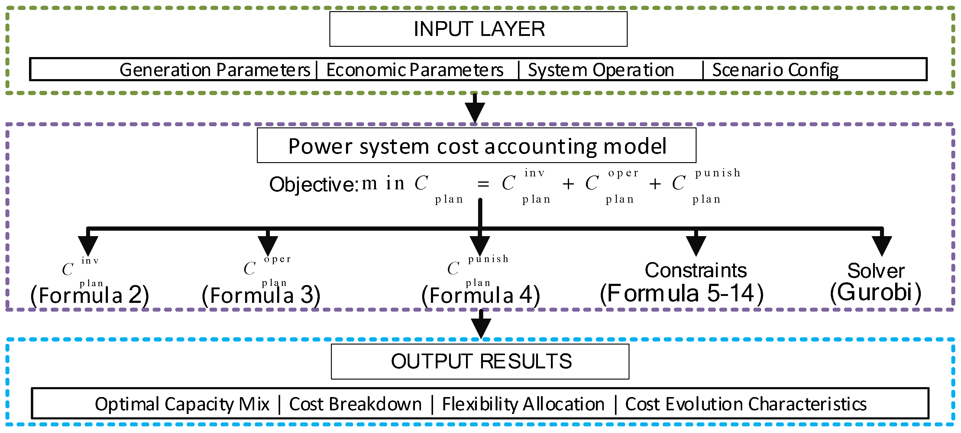
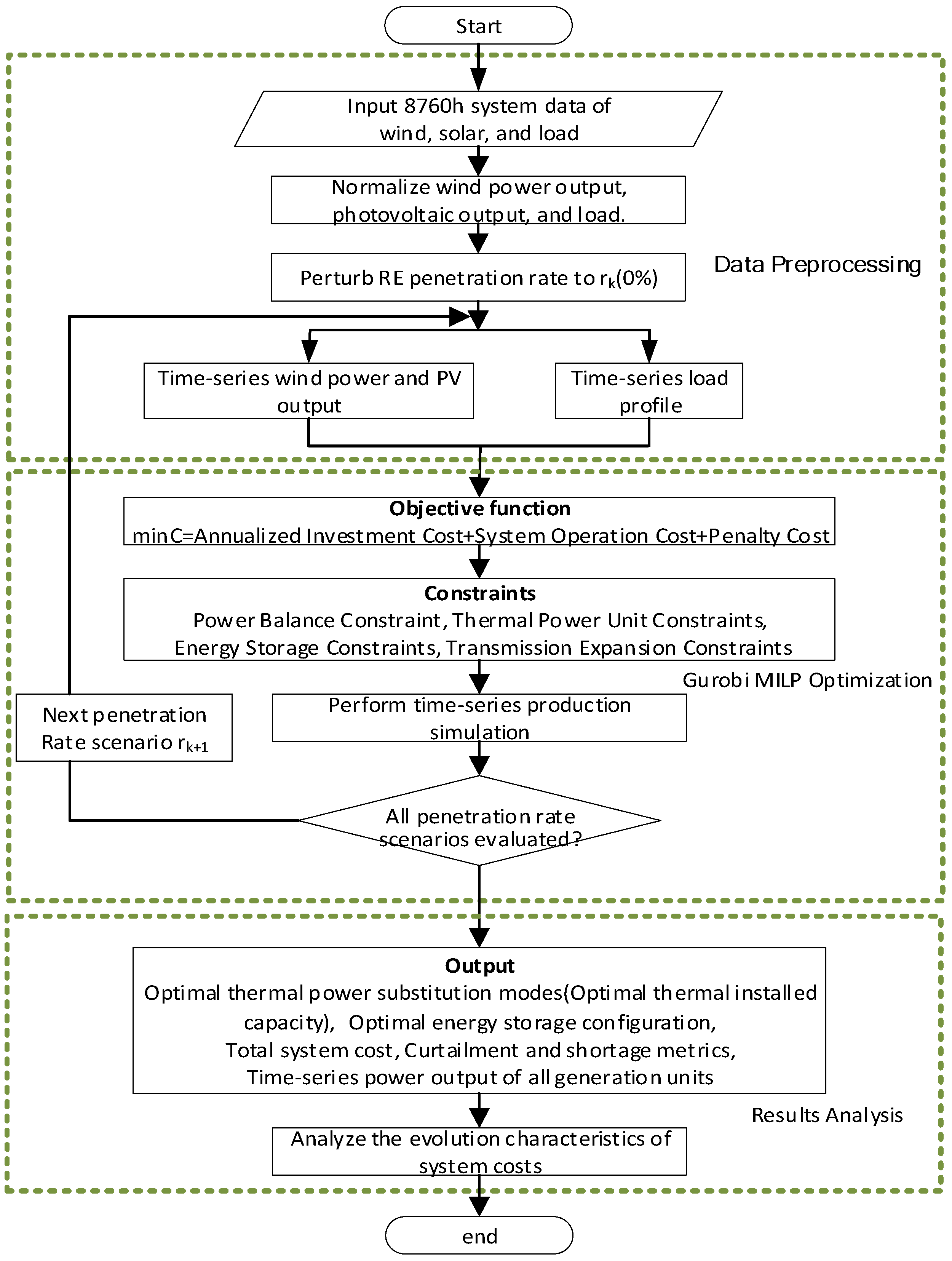
The framework of the power system cost accounting model established in this paper is illustrated in Figure 4. As shown, the formulation comprises three core cost components—investment cost, operation cost, and penalty cost—subject to a set of technical and operational constraints.

The model established in this chapter serves as the theoretical foundation for the Garver-6 system case study presented in Section 4. Detailed specifications of variables, parameters, and equations are provided in the subsequent subsections.

3.2. Objective Function

The proposed model aims to minimize the total annualized system cost under varying renewable energy penetration rates. The total cost comprises three components: annualized investment cost for generation and storage capacity, system operation cost including fuel and maintenance expenditures, and penalty cost incurred from load shedding and renewable energy curtailment. The objective function is formulated as follows:

$$\min C_{\mathrm{plan}}=C_{\mathrm{plan}}^{\mathrm{inv}}+C_{\mathrm{plan}}^{\mathrm{oper}}+C_{\mathrm{plan}}^{\mathrm{punish}}$$

(1)

where $C_{\mathrm{plan}}^{\mathrm{inv}}$, $C_{\mathrm{plan}}^{\mathrm{oper}}$, and $C_{\mathrm{plan}}^{\mathrm{punish}}$ denote the annualized investment cost, system operation cost, and penalty cost, respectively. The detailed formulations of these three components are provided in Equations (2)–(4).

3.2.1. Annualized Investment Cost

The annualized investment cost $C_{\mathrm{plan}}^{\mathrm{inv}}$ converts the upfront capital expenditure of generation and storage capacity into an equivalent annual cost over the planning horizon, which is expressed as follows:

$$C_{\mathrm{plan}}^{\mathrm{inv}}={\displaystyle \frac{\eta {(1+\eta )}^{N_{\mathrm{s}}}}{{(1+\eta )}^{N_{\mathrm{s}}}-1}}(c_{\mathrm{gen}}^{\mathrm{inv}}{P}_{\mathrm{gen}}+c_{\mathrm{wind}}^{\mathrm{inv}}{P}_{\mathrm{wind}}+c_{\mathrm{sun}}^{\mathrm{inv}}{P}_{\mathrm{sun}}+c_{\mathrm{pess}}^{\mathrm{inv}}{P}_{\mathrm{e}}+c_{\mathrm{ess}}^{\mathrm{inv}}{E}_{\mathrm{e}})$$

(2)

where $c_{\mathrm{gen}}^{\mathrm{inv}}$, $c_{\mathrm{wind}}^{\mathrm{inv}}$, $c_{\mathrm{sun}}^{\mathrm{inv}}$, $c_{\mathrm{pess}}^{\mathrm{inv}}$ and $c_{\mathrm{ess}}^{\mathrm{inv}}$ are the unit investment cost coefficients of thermal power, wind, photovoltaic, energy storage power and energy storage capacity, respectively (yuan/kW or yuan/kWh); P_gen, P_wind, P_sun, and P_e denote the installed capacity of each technology (kW); E_e is the energy storage capacity (kWh); η is the discount rate (5%); N_s is the planning horizon (15 years).

3.2.2. System Operation Cost

The system operation cost $C_{\mathrm{plan}}^{\mathrm{oper}}$ accounts for the annual expenditures on fuel consumption, environmental treatment, and operation and maintenance, which is given by the following:

$$C_{\mathrm{plan}}^{\mathrm{oper}}=({\alpha }_g+{\beta }_g)P_{g,t}+P_{\mathrm{gen}}{R}_{\mathrm{g}}+P_{\mathrm{wind}}{R}_{\mathrm{w}}+P_{\mathrm{sun}}{R}_{\mathrm{s}}+(c_{\mathrm{pess}}^{\mathrm{inv}}{P}_{\mathrm{e}}+c_{\mathrm{ess}}^{\mathrm{inv}}{E}_{\mathrm{e}}){\mathrm{R}}_{\mathrm{e}}$$

(3)

where α_g and β_g are the fuel and environmental cost coefficients of thermal units (yuan/kWh); P_g,t is the output of the thermal power unit at time t; R_g, R_w, R_s, and R_e are the operation and maintenance cost coefficients (yuan/kW).

3.2.3. Penalty Cost

The penalty cost $C_{\mathrm{plan}}^{\mathrm{punish}}$ captures the economic penalties associated with power shortage and renewable energy curtailment, which is formulated as follows:

$$C_{\mathrm{plan}}^{\mathrm{punish}}={\delta }^{\mathrm{d}}{D}_{n,t}^{\mathrm{cut}}+{\delta }^{\mathrm{w}}{P}_{w,t}^{\mathrm{cut}}+{\delta }^{\mathrm{pv}}{P}_{pv,t}^{\mathrm{cut}} \forall t\in T$$

(4)

where δ^d, δ^w, δ^pv are the penalty coefficients for power shortage, wind curtailment, and photovoltaic curtailment, respectively (yuan/kWh); $D_{n,t}^{\mathrm{cut}}$ is the power shortage at time $t$ (kW); $P_{w,t}^{\mathrm{cut}}$, $P_{pv,t}^{\mathrm{cut}}$ are the curtailed wind and photovoltaic power at time $t$ (kW).

3.3. Constraints

The minimization of the objective function is subject to a set of technical and operational constraints that ensure the feasibility and reliability of the system operation. These constraints govern power balance, generation limits, ramping capabilities, transmission capacity, energy storage dynamics, and network expansion limits. The detailed formulations are presented in the following subsections.

3.3.1. Power Balance Constraint

The power balance constraint ensures that generation and storage discharge equal load and storage charging at every time step, accounting for power shortage and renewable curtailment:

$$P_{g,t}+P_{w,t}+P_{pv,t}+P_{e,t}^{\mathrm{dis}}-P_{e,t}^{cha}=D_{n,t}-D_{n,t}^{\mathrm{cut}}-P_{w,t}^{\mathrm{cut}}-P_{pv,t}^{\mathrm{cut}} \forall t\in T$$

(5)

where P_g,t is the output of the thermal power unit at time t; P_w,t and P_pv,t are the wind and photovoltaic power outputs at time t; $P_{e,t}^{\mathrm{dis}}$ and $P_{e,t}^{cha}$ are the discharging and charging power of energy storage at time t; D_n,t is the system load at time t; T is the set of time periods.

3.3.2. Generation Limits of Thermal Power Units

The output of each thermal power unit is constrained within its technical minimum and maximum limits:

$$P_g^{\min }\le P_{g,t}\le P_g^{\max } \forall t\in T$$

(6)

where $P_g^{\min }$ and $P_{g,t}^{\max }$ are the minimum and maximum output limits of the thermal power unit.

3.3.3. Ramping Constraints of the Thermal Power Unit

The ramping constraints limit the rate at which thermal units can increase or decrease their output between consecutive time periods:

$$-\mu P_{\mathrm{gen}}\le P_{g,t+1}-P_{g,t}\le \mu P_{\mathrm{gen}} \forall t\in T$$

(7)

where μ is the ramping rate coefficient of the thermal power unit (50%).

3.3.4. Energy Storage Constraints

Lithium-ion battery energy storage is considered as the primary flexibility resource. Lithium-ion batteries offer advantages including fast response, high energy density, and high cycle efficiency, making them the most widely deployed electrochemical storage technology in modern power systems. The operation of energy storage is governed by power limits, state-of-charge dynamics, and daily energy balance requirements:

$$0\le P_{e,t}^{\mathrm{dis}}\le P_e , 0\le P_{e,t}^{\mathrm{cha}}\le P_e \forall t\in T$$

(8)

$$SO{C}_t=SO{C}_{t-1}+{\eta }_e{P}_{e,t}^{\mathrm{cha}}-P_{e,t}^{\mathrm{dis}}/{\eta }_e \forall t\in T$$

(9)

$$SO{C}_{\min }\le SO{C}_t\le SO{C}_{\max } \forall t\in T$$

(10)

$$SOC(24)=SO{C}_{ini}$$

(11)

where $P_{e,t}^{\mathrm{dis}}$ and $P_{e,t}^{\mathrm{cha}}$ represent the discharging power and charging power of the energy storage; η_e represents the charging/discharging efficiency of the energy storage (taken as 0.95); SOC_t and SOC_t−1 represent the state of charge of the energy storage at time t and time t − 1; SOC_min and SOC_max represent the minimum and maximum state of charge limits of the energy storage (taken as 10% and 90%); SOC_ini represents the initial state of charge of the energy storage (taken as 50%).

3.3.5. Available Transfer Capability Limitation of Lines (DC Power Flow)

The power flow on each transmission line is governed by the DC power flow model and must respect the line’s thermal capacity limits (The supplementary content is shown in Appendix A):

$$B{\theta }_t=P_{\mathrm{g},t}+P_{\mathrm{w},t}+P_{pv,t}+P_{e,t}^{\mathrm{dis}}-P_{e,t}^{cha}-D_{n,t} \forall t\in T$$

(12)

where B is the node admittance matrix (susceptance matrix); θ_t is the vector of nodal voltage phase angles at time t.

3.3.6. New Line Construction Constraints

The number of new transmission lines that can be constructed is subject to corridor capacity limits:

$$0\le x_{ij}^{\mathrm{new}}\le N_{i,j}^{\max } \forall (i,j)\in {\mathrm{\Omega }}_{\mathrm{line}}$$

(13)

where $x_{ij}^{\mathrm{new}}$ is the number of new transmission lines constructed in corridor (i, j); $N_{i,j}^{\max }$ is the maximum allowable number of new lines in that corridor; Ω_line is the set of candidate transmission corridors.

3.3.7. Transmission Line Power Flow Constraints

The power flow on each transmission corridor is limited by the total capacity of existing and newly constructed lines:

$$\left|P_{ij,t}\right|\le (x_{ij}^0+x_{ij}^{\mathrm{new}})\left|P_{ij}^{\max }\right| \forall (i,j)\in {\mathrm{\Omega }}_{\mathrm{line}}\hspace{1em}\forall t\in T$$

(14)

where P_ij,t is the actual power flow on corridor (i, j) at time t; $P_{ij}^{\max }$ is the maximum capacity of a single transmission line in that corridor, $x_{ij}^0$ is the number of existing lines; $x_{ij}^{\mathrm{new}}$ is the number of newly constructed lines.

3.4. Solving Procedure

The solution methodology employs a two-level framework that couples scenario-based parameter analysis at the outer level with Mixed Integer Linear Programming (MILP) optimization at the inner level. The outer level systematically varies the renewable energy penetration rate to characterize cost evolution trajectories. For each penetration scenario, the inner level solves a full MILP problem to optimality using the Gurobi solver 10.0, determining the optimal thermal capacity, energy storage configuration, and hourly dispatch decisions. The overall solution framework is illustrated in Figure 5.

The solving steps are as follows.

• Step 1: Data Input and Preprocessing

Input 8760 h system data of wind power, photovoltaic generation, and load. Normalize the wind power output, photovoltaic output, and load profiles. Perturb (or adjust) the renewable energy penetration rate to the initial stage $r_k$ (e.g., 0%). Complete data preprocessing to obtain time-series wind/PV output curves and time-series load profiles.

• Step 2: Optimization Model Formulation

Formulate an optimization model aimed at minimizing total system cost. The objective function comprises three components: annualized investment cost, system operation cost, and penalty cost. Constraints include power balance constraints, thermal power unit constraints, energy storage constraints, and transmission expansion constraints. The model is solved using the Gurobi optimizer via Mixed Integer Linear Programming (MILP).

• Step 3: Time-Series Production Simulation

Perform time-series production simulation to evaluate the system operating state under the current penetration scenario.

• Step 4: Scenario Iteration Check

Check whether all predefined penetration rate scenarios have been evaluated. If No, update to the next penetration scenario $r_{k+1}$ and return to Step 3. If Yes, proceed to Step 5.

• Step 5: Output Results

Output the optimal planning scheme for each penetration scenario, including the following: optimal thermal power substitution modes (optimal thermal installed capacity), optimal energy storage configuration, total system cost, curtailment and shortage metrics, and time-series power output of all generation units.

• Step 6: Results Analysis

Compile the results across all scenarios and analyze the evolution characteristics of the system costs with increasing renewable energy penetration. Complete the results analysis.

4. Case Study

To validate the effectiveness of the proposed cost evolution framework and to investigate the mechanism by which renewable energy penetration influences system costs, this section presents a comprehensive case study based on the modified Garver-6 test system. The analysis encompasses multiple renewable energy penetration rate scenarios, progressively transitioning from a thermal-dominated baseline configuration to a high-renewable future scenario. The calculation parameters are first provided, followed by a comparison of different thermal power substitution modes and the determination of the optimal thermal substitution strategy. Finally, the system cost evolution characteristics are derived and analyzed.

4.1. Base Data

In order to analyze the influence of the change of the renewable energy penetration rate on the total cost of the power system and obtain the evolution path of the system cost, this paper uses the measured wind and solar load data of a province in Northeast China in recent years to analyze as an example.

Perturb the renewable energy penetration rate with 10% as the step size, simulate the system cost, and analyze its change trend under the condition of penetration rate from 0% to 100% through time series production simulation. The planning period of this paper is 15 years, and the discount rate is 5%. The calculation parameters used are shown in

Table 2. Design conditions.

Parameter	Numerical Value	Parameter	Numerical Value
Thermal power construction cost	50,000 yuan/kW	Thermal power operation and maintenance cost	3000 yuan/kW
Wind power construction cost	54,000 yuan/kW	Fuel cost	2.8 yuan/kW
Photovoltaic construction cost	33,000 yuan/kW	Thermal power environmental protection cost	3000 yuan/kW
Energy storage power cost	1000 yuan/kW	Wind power operation and maintenance cost	1500 yuan/kW
Energy storage capacity cost	6000 yuan/kWh	Photovoltaic operation and maintenance cost	2000 yuan/kW
Curtailment penalty	830 yuan/kWh	Energy storage operation and maintenance cost coefficient	1.05
Power shortage penalty	100 yuan/kWh	Transmission line construction cost	1000 yuan/kW/km

.

4.2. Analysis of Cost Evolution Trend Under a 1:1 Replacement Scenario

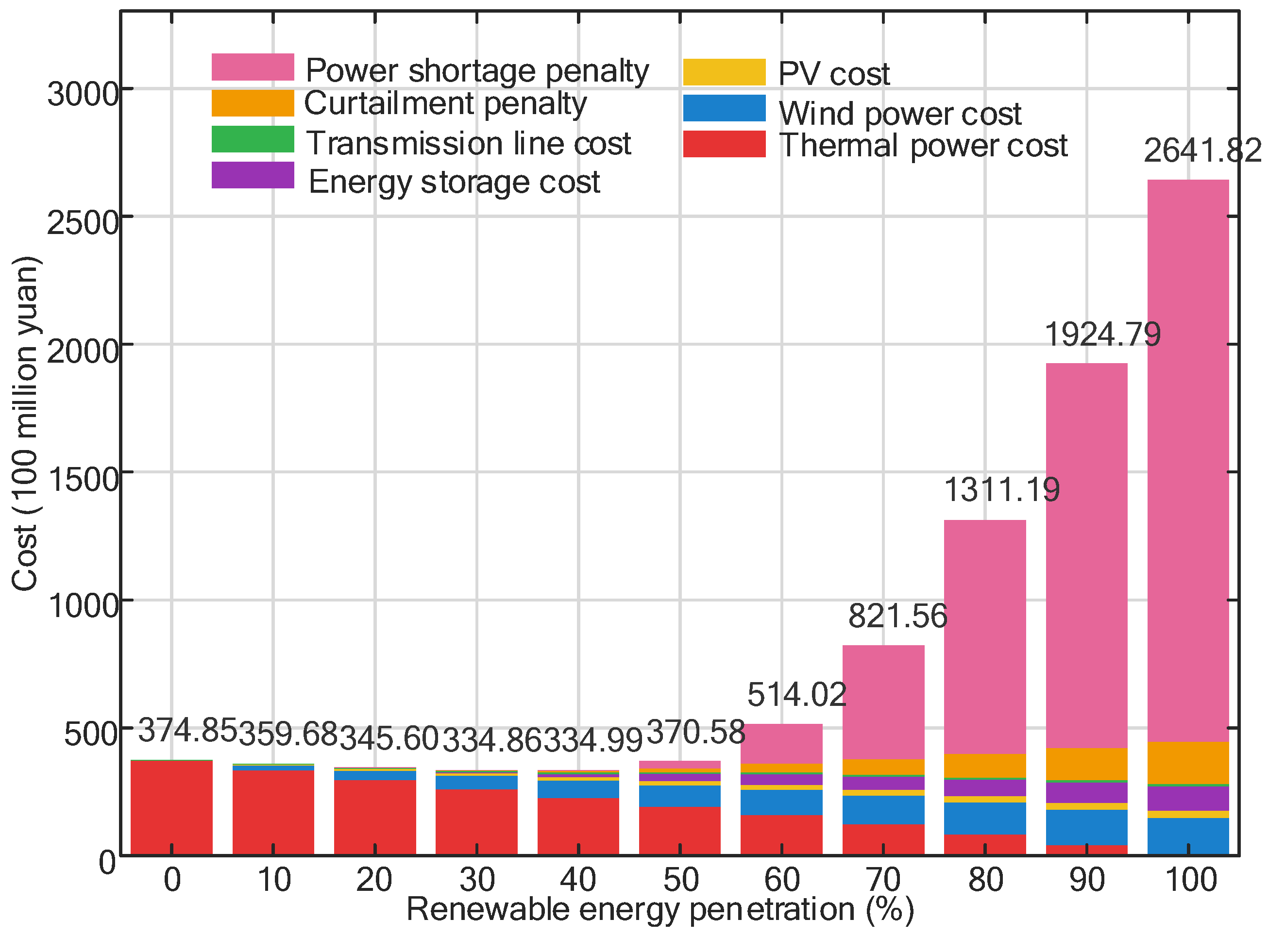
Through the above steps, the production simulation is solved under different renewable energy penetration rates, and the cost composition and changes in the system are obtained as shown in Figure 6.

From Figure 6, it can be seen that with the increase of penetration rate, the total cost of the system shows a trend of decreasing first and then increasing. At 30%, the total cost is the lowest at 334.86 billion yuan. The main reason is that renewable energy sources with relatively low costs such as wind power and photovoltaics are connected to the power system, resulting in the compression of the output space of the thermal power units and the continuous decline of the thermal power costs. It decreased from yuan 37.23 billion at the initial 0% penetration rate to yuan 0 billion at the 100% penetration rate. Due to the 100% penetration rate, the installed capacity of thermal power is 0, thermal power no longer provides electricity, so the cost is 0 billion yuan.

When the penetration rate is low, it is not necessary to configure short-term energy storage or configure a small amount of short-term energy storage to maintain the stability of the system, and there are fewer violations such as load shedding; that is, the increase in the adjustment cost of wind, light, and power connected to the system is less than the reduction in the cost of the thermal power output. Therefore, the total cost of the system decreases from 374.85 billion yuan at 0% to 334.86 billion yuan at 30%, a total decrease of 3.999 billion yuan; with the gradual increase of penetration rate, the output of wind power and photovoltaic power in the system increases. It is necessary to configure more short-term energy storage and expand more lines to increase the flexibility of the system, ensure the smooth transmission of power, and reduce the lack of peak shaving and the blocking of transmission lines. With the increase of the penetration rate, the energy storage cost increases monotonously, reaching a maximum of 9.49 billion yuan when the penetration rate is 100%. The number of line expansions increases, and the expansion center of gravity shifts to wind power and photovoltaic nodes. At the same time, the adjustment cost and the cost of scenery construction have risen sharply, and there are also more load shedding phenomena, so the total cost of the system has increased by up to 230.696 billion yuan.

Based on the above analysis, under this thermal power substitution mode, the total cost of the system and the cost of electricity are first decreased and then increased, and the minimum value is obtained at 30% penetration rate. On the one hand, wind power and photovoltaic renewable energy, as a ‘double-edged sword’, reduce the system cost while causing the system adjustment cost to rise. As the penetration rate increases, the difference between the two increases, and the total system cost increases; on the other hand, renewable energy is gradually replacing thermal power, the installed capacity of thermal power is declining, the system has no power supply, and there is no flexible resource to solve the problem of long-term abandonment and shortage of electricity. Therefore, a large number of abandonments and shortages of electricity have a great impact on the system cost.

4.3. Comparative Analysis of Cost Evolution Law Under Different Alternative Methods

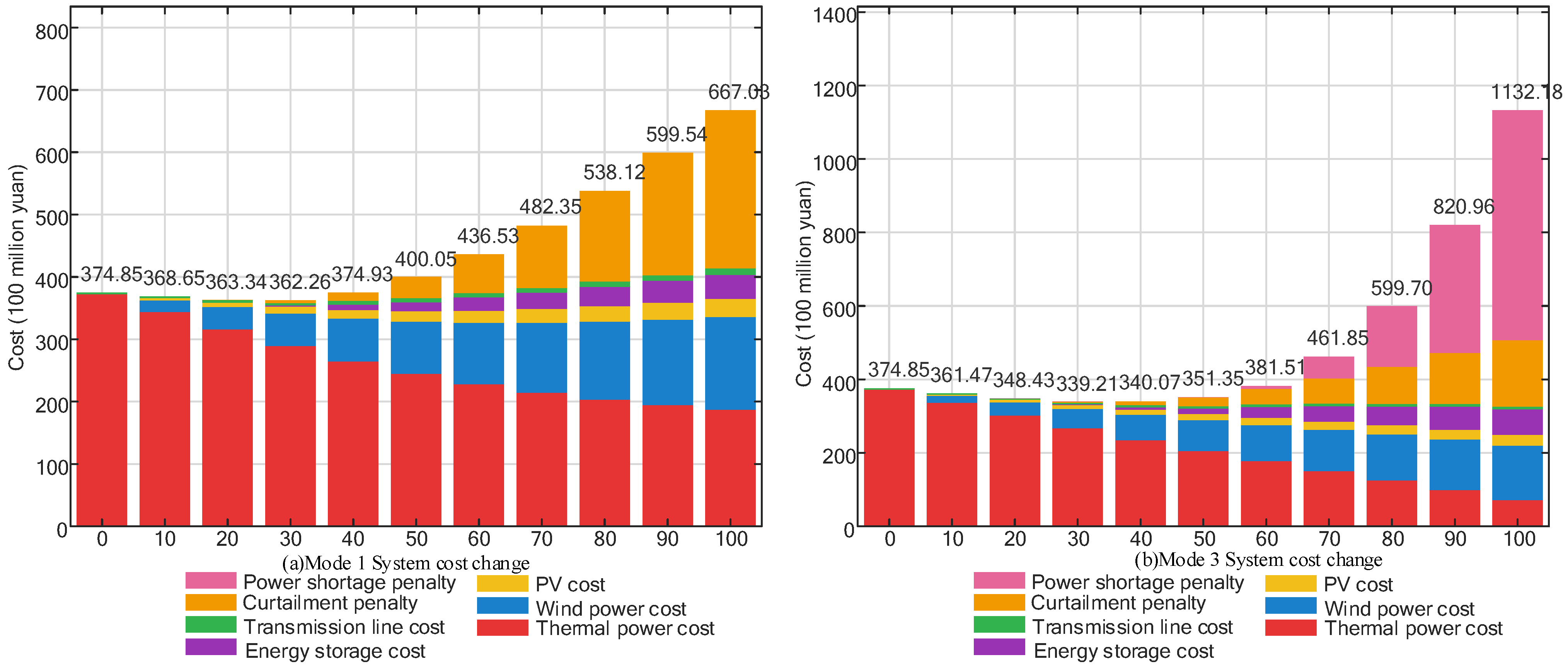
According to the comparison between mode 1 and mode 3 as shown in Table 1, the influence of different thermal power substitution modes on system cost is analyzed.

From Figure 7, it can be seen that under the two different thermal power substitution modes, the change of the system cost composition is quite different, but the overall change trend is first to decrease and then increase, and both reach the lowest value at 30% penetration rate, which is 362.26 billion yuan and 339.21 billion yuan respectively.

(1)

Analysis of system cost change in mode 1

First, in mode 1, because the installed capacity of the thermal power units is sufficient and does not change with the increase of the renewable energy penetration rate, the system is flexible enough at this time. As the main provider of flexibility, the thermal power can increase or decrease the output as the system needs, and the cost of thermal power is still an important part of the total cost of the system, accounting for a high proportion. However, due to its limitation of minimum output, the downward flexibility of the system is low, and problems such as inability to absorb wind power and photovoltaics occur at a high penetration rate, resulting in a continuous increase in the system’s abandonment rate and a monotonous increase in the abandonment penalty. At 100% penetration rate, it is up to 25.32 billion yuan; however, the system has sufficient upward flexibility, and no power shortage occurs. The specific energy storage configuration and line expansion are shown in

Table 3. Mode 1. Energy storage configuration.

RE Penetration Rate	Energy Storage Power/10,000 kW	Energy Storage Capacity/10,000 kWh	Energy Storage Cost/100 Million Yuan
0%	0	0	0
10%	0	0	0
20%	0	0	0
30%	174.8	342.5	1.9
40%	482.6	1670.4	8.9
50%	766.9	2685.6	14.2
60%	1009.0	4081.5	21.5
70%	1211.4	5022.6	26.4
80%	1445.3	5944.5	31.3
90%	1627.0	6792.8	35.7
100%	1644.6	7361.9	38.6

and

Table 4. Mode 1. Line expansion.

RE Penetration Rate	Line 1–2	Line 1–4	Line 1–5	Line 2–3	Line 2–4	Line 3–5	Line 2–6	Line 3–6	Line 4–6
0%	1	1	1	1	0	0	0	0	0
10%	1	1	1	1	0	0	0	0	0
20%	1	1	1	1	0	1	1	0	1
30%	1	1	1	1	0	1	1	0	1
40%	1	1	1	1	0	1	2	1	2
50%	1	1	1	1	0	1	3	1	2
60%	1	1	1	1	0	1	3	1	2
70%	1	1	1	1	0	1	3	1	3
80%	1	1	1	1	1	1	3	1	4
90%	1	1	1	1	1	1	3	1	4
100%	1	1	1	1	1	1	3	2	5

. Although the installed capacity of thermal power is sufficient and the system flexibility is high, the configuration of energy storage is still an effective means to solve the unbalanced power, and it is also of least cost. The focus of line expansion is still shifting to renewable energy nodes.

(2)

Analysis of system cost change in mode 3

In mode 3, it can be seen from Figure 7b that in the process of gradually reducing the installed capacity of thermal power, the power shortage in the system is aggravated. When the penetration rate is 70% and above, the power shortage penalty has a huge impact on the total cost of the system, accounting for the most cost. As the penetration rate increases, the upward and downward flexibility in the system decreases, and the penalty for power abandonment also increases. As a flexible resource, short-term energy storage still cannot solve the uneven distribution of renewable energy power in the season and can only solve the flexibility shortage on some days, resulting in a sharp rise in cost after the penetration rate is 30%. The specific energy storage configuration and line expansion are shown in

Table 5. Mode 3. Energy storage configuration.

RE Penetration Rate	Energy Storage Power/10,000 kW	Energy Storage Capacity/10,000 kWh	Energy Storage Cost/100 Million Yuan
0%	0	0	0
10%	0	0	0
20%	0	0	0
30%	189.9	256	1.5
40%	390.7	1235.4	6.6
50%	761.2	2840.2	15
60%	1034.5	5692.8	29.7
70%	1286.3	8078.4	41.9
80%	1534.5	9814.1	50.9
90%	1623	12,086.2	62.5
100%	1795.8	13,356.3	69

and

Table 6. Mode 3. Line expansion.

RE Penetration Rate	Line 1–2	Line 1–4	Line 1–5	Line 2–3	Line 2–4	Line 3–5	Line 2–6	Line 3–6	Line 4–6
0%	1	1	1	1	0	0	0	0	0
10%	1	1	1	1	0	0	0	0	0
20%	1	1	1	1	0	0	1	0	1
30%	1	1	1	1	0	1	2	1	2
40%	1	1	1	1	0	1	2	1	2
50%	1	1	1	1	0	1	3	1	2
60%	0	1	1	1	1	1	3	1	2
70%	0	1	1	1	1	1	3	1	3
80%	0	1	1	2	0	1	3	1	4
90%	0	1	1	2	0	2	3	1	4
100%	0	1	0	2	0	2	3	1	5

.

In summary, under different thermal power installed capacity substitution methods, the cost evolution law of the system is similar, showing a trend of decreasing first and then increasing. At a low penetration rate, the total system cost of different thermal power installed capacity substitution methods is less different. The main reason is that the thermal power installed capacity is high and basically meets the load. At the same time, the wind power photovoltaic output is low, and the system just needs to pay less adjustment cost to ensure the system power balance and to reduce the occurrence of unbalanced events. With the further increase of the penetration rate, the different alternatives begin to appear, which is embodied in the contradiction between the installed capacity of thermal power and the punishment of power abandonment and power shortage. When the installed capacity of the thermal power is redundant, the system abandonment penalty is high due to the influence of the minimum output constraint. When the installed capacity of the thermal power is insufficient, the load cannot be supplied, and the penalty of system power shortage is high.

4.4. Cost Evolution Trend Under Optimal Thermal Power Substitution Mode

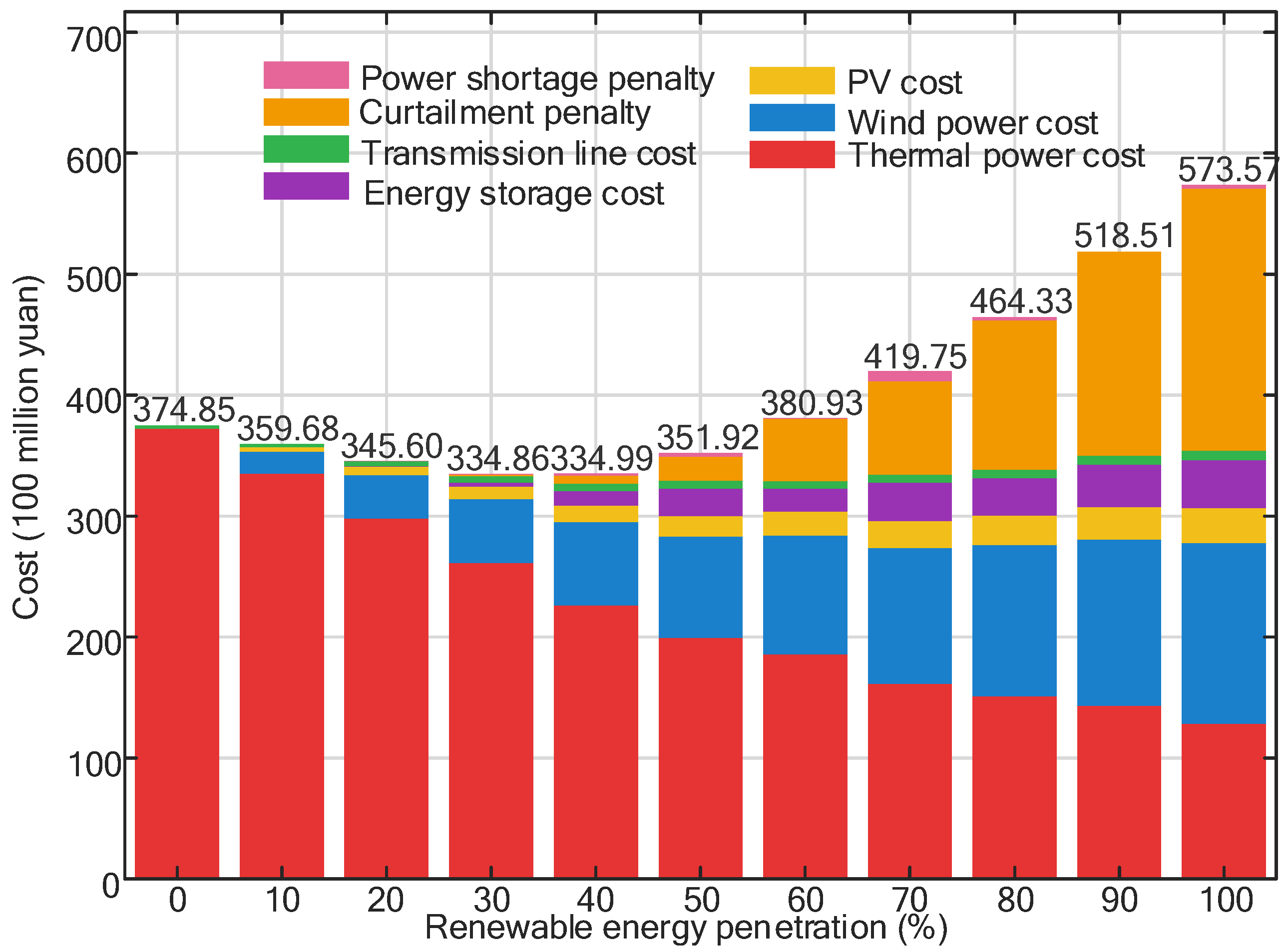
Considering the relationship between the replacement ratio of thermal power installed capacity and the system cost under different penetration rates, the optimal replacement ratio of thermal power installed capacity and the total cost are obtained as shown in

Table 7. Optimal thermal power installed capacity substitution ratio and total cost under different penetration rates.

RE Penetration Rate	Replacement Mode	Thermal Power Installed Capacity/10,000 kW	Total Cost/100 Million Yuan
0%	/	2111	374.9
10%	1:1	1900	359.7
20%	1:1	1689	345.6
30%	1:1	1478	334.9
40%	1:1	1267	335.0
50%	0.9:1	1161	351.9
60%	0.7:1	1225	380.9
70%	0.7:1	1077	419.7
80%	0.6:1	1098	464.3
90%	0.5:1	1161	518.5
100%	0.5:1	1056	573.6

and Figure 8 by solving all the above methods.

Through Table 7 and Figure 8, it can be seen that the trend of the total cost of the system under the optimal replacement ratio of thermal power installed capacity is still first decreasing and then increasing, and the lowest is 334.9 billion yuan when the penetration rate is 30%. However, in the process of rising system costs, it can be seen that the installed capacity of thermal power is almost maintained between 10–12 million kW. Although having a large number of wind power and photovoltaic access sources, the thermal power installed capacity to maintain a high level to increase the flexibility of the system is still a good choice; the thermal power installed capacity alternative to the unit capacity of thermal power to replace more renewable energy change also shows the importance of thermal power when the flexibility of resources is limited under a high penetration rate. The specific energy storage configuration is shown in

Table 8. Energy storage configuration of the optimal alternative method.

RE Penetration Rate	Energy Storage Power/10,000 kW	Energy Storage Capacity/10,000 kWh	Energy Storage Cost/100 Million Yuan
0%	0	0	0
10%	0	0	0
20%	16.8	22.1	0.1
30%	250	596.1	3.2
40%	513.2	2248.5	11.8
50%	832.2	4364.8	22.8
60%	957.9	3658.2	19.3
70%	1271.9	6111.6	32
80%	1458	5803.6	30.6
90%	1451	6718.9	35.2
100%	1676	7603.9	39.9

. As a flexible resource, energy storage can solve some unbalanced events, but the cost of energy storage is increasing steadily.

4.5. Sensitivity Analysis of Key Parameters

To assess the robustness of the identified cost evolution characteristics and optimal thermal power substitution modes, a sensitivity analysis was conducted with respect to the investment costs of wind and photovoltaic generation. Two additional scenarios were considered.

Scenario S1: Wind and PV investment costs are reduced by 10% relative to the reference case.

Scenario S2: Wind and PV investment costs are reduced by 20% relative to the reference case.

The reference case uses the original cost assumptions as presented in Table 2.

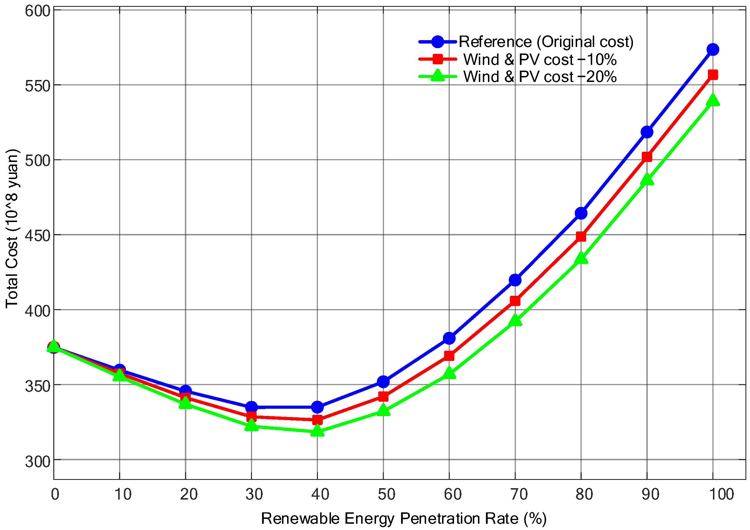
Figure 9 presents the evolution of the total annualized system cost across the three scenarios as renewable penetration increases from 0% to 100%. The following observations can be made.

In all three scenarios, the system cost exhibits the same characteristic “U-shaped” trajectory—initially decreasing as low-cost renewable energy displaces thermal generation, reaching a minimum, and subsequently increasing as flexibility resource requirements (energy storage and transmission expansion) become dominant. The overall shape of the cost curve remains unchanged, confirming that the underlying cost structure is driven primarily by the physical constraints of the system rather than the absolute level of the renewable investment costs. As expected, reducing wind and PV investment costs lowers the total system cost across all penetration levels. The magnitude of the reduction is approximately proportional to the share of renewable investment in the total cost. Delay of the optimal penetration point: The penetration rate at which the minimum system cost occurs shifts to the right as the renewable costs decrease. Specifically, the optimal penetration rate increases from 30% in the reference case to 40% in S1 and S2. This indicates that lower renewable costs make higher penetration levels economically attractive before flexibility constraints begin to dominate.

Table 9. Impact of wind and PV cost reduction on optimal thermal power substitution mode.

RE Penetration Rate	Reference (Original Cost)	Scenario S1 (Cost −10%)	Scenario S2 (Cost −20%)
0%	/	/	/
10%	1:1	1:1	1:1
20%	1:1	1:1	1:1
30%	1:1	1:1	1:1
40%	1:1	1:1	1:1
50%	0.9:1	1:1	1:1
60%	0.7:1	0.7:1	0.8:1
70%	0.7:1	0.7:1	0.7:1
80%	0.6:1	0.6:1	0.6:1
90%	0.5:1	0.5:1	0.5:1
100%	0.5:1	0.5:1	0.5:1

compares the optimal thermal power substitution mode selected under each renewable penetration level for the three cost scenarios.

The optimal substitution mode remains largely consistent across the three scenarios, particularly at low and high penetration extremes. This suggests that the choice of substitution strategy is governed more by system flexibility constraints than by renewable cost assumptions.

Minor differences are observed in the intermediate penetration range (50–60%), where the cost differential between adjacent substitution modes is relatively small. In this region, Scenarios S1 and S2 exhibit increased optimal energy storage deployment compared to the reference case. The additional storage capacity enhances system flexibility, enabling lower renewable energy costs to support a more aggressive thermal substitution strategy—that is, accommodating greater renewable generation with less thermal capacity. Consequently, lower renewable costs tend to favor lower modes over a wider range of penetration levels.

Overall, the sensitivity analysis confirms that the main findings of this study are robust to the reasonable variations in the renewable energy investment cost assumptions. The U-shaped cost evolution trajectory remains qualitatively unchanged; The optimal substitution modes are stable at the extremes and exhibit only localized, explainable variations in the intermediate penetration range.

These results reinforce the validity of the proposed cost accounting framework and the identified optimal thermal power substitution strategies.

5. Conclusions

With the increasing proportion of renewable energy grid-connected, the source–load operation mode in the traditional power system is difficult to sustain, and the flexibility demand increases sharply. Based on the actual development and future trend of China’s new power system, this paper analyzes the changes of system flexibility and the factors affecting system cost and proposes a cost evolution model considering the development of the new power system in the future. Through the analysis of examples, the differences and problems of system cost evolution under different thermal power installed capacity substitution ratios are compared, and the optimal thermal power installed capacity substitution ratio under different penetration rates is obtained. The following conclusions are obtained:

• From the perspective of the daily penetration rate, in the process of increasing wind power and photovoltaic penetration rate, the installed capacity of thermal power is being gradually reduced, and the flexibility of the system is becoming sharply reduced. At the same time, there is a problem of insufficient flexibility in up-regulation and down-regulation, which needs to be solved by configuring energy storage.
• The main factors affecting the system cost are the cost of reducing the output of compressed thermal power after the integration of wind power and photovoltaic power and the cost of increasing the allocation of flexible resources when the system flexibility is in short supply during the change of the renewable energy penetration rate. At the same time, the replacement ratio of the installed capacity of different thermal power units also has a great impact on the system cost.
• The example analysis shows that with the increase of the penetration rate, the system cost shows a trend of first decreasing and then increasing. When the installed capacity of the thermal power is balanced with the flexible resource allocation, the system cost is the lowest. The substitution method of thermal power installed capacity is also changing to replace more renewable energy with less thermal power, indicating that the system still needs a certain thermal power to ensure the stability of the system at a high penetration rate.
• Finally, while renewable energy penetration continues to increase, thermal power plants still play an indispensable role as the main backbone of the system, providing essential flexibility and reliability services that cannot yet be fully replaced by renewable generation or energy storage.

The Garver-6 system used in this study is suitable for methodological validation but is too small to capture the geographic diversity of wind and solar power, realistic congestion models, or the variety of flexibility products in large-scale power systems. Future research will focus on the following two directions:

• The proposed model will be tested on larger, more realistic test systems (e.g., IEEE 118-bus system or a provincial-level power system in China) with multi-region modeling to capture the spatial and temporal variability of wind and solar resources.
• The current deterministic framework will be extended to incorporate stochastic or robust optimization techniques to account for the variability and uncertainty of renewable energy generation and load demand, which is critical for real-world applications.
• We note that incorporating shiftable loads, price-responsive demand, and electric vehicle charging flexibility would enable a more comprehensive assessment of the system cost evolution under high renewable penetration.