Article

An Adaptive Switching Method for Sensorless Startup of High-Speed SPMSM Based on the Cosine of the Angle Error

by
Wei Chen
1,2,*,
Shiwei Zhang
1,
Zhiqiang Wang
1,
Xinmin Li
1,
Shuxin Xiao
3 and
Zhezhun Xu
4
1
School of Electrical Engineering, Tiangong University, Tianjin 300387, China
2
Zhejiang University Advanced Electrical Equipment Innovation Center, Hangzhou 311107, China
3
China North Engine Research Institute, National Key Laboratory of Vehicle Power System, Tianjin 300405, China
4
Technical Center of Hangzhou Customs, Hangzhou 310007, China
*
Author to whom correspondence should be addressed.
Energies 2026, 19(9), 2140; https://doi.org/10.3390/en19092140
Submission received: 13 March 2026 / Revised: 20 April 2026 / Accepted: 24 April 2026 / Published: 29 April 2026

Abstract

To address the current surge and speed fluctuation that occur when high-speed surface-mounted permanent magnet synchronous motors (HSPMSMs) switch from I-f open-loop control to sensorless closed-loop control, an adaptive switching method based on the cosine of the angle error is proposed. In this method, the angle error between the I-f open-loop reference angle and the angle estimated by the sensorless observer serves as the regulating variable, and its cosine is introduced to construct an adaptive attenuation factor, so that the rate of current reduction can vary continuously with the angle error. Specifically, a relatively large rate of current reduction is generated in the early stage of the switching process, when the angle error is large, to shorten the switching time. As the angle error decreases, the rate of current reduction is gradually lowered, allowing the current regulation process to better match the convergence process of the angle error and thereby improving switching stability. The proposed switching method is validated on a high-speed air compressor experimental platform. The experimental results show that the proposed method can shorten the switching time, reduce the current surge and speed fluctuation at switching, and exhibit good robustness under varying operating conditions.

1. Introduction

High-speed permanent magnet synchronous motors (HPMSMs) have been widely applied in industrial compressors, aerospace systems, and other fields due to their high power density, wide speed range, and excellent dynamic response [1,2]. The stable operation of HPMSMs relies on rotor position information, while high-speed operating environments impose more stringent requirements on the installation and operation of position sensors. Therefore, sensorless control technologies for HPMSMs have attracted significant attention [3,4].
Different sensorless control methods are typically employed for HPMSMs in different speed ranges [5]. In the zero- and low-speed range, commonly used methods include speed closed-loop control based on high-frequency signal injection [6] and speed open-loop control based on V/f [7] and I-f [8,9,10,11,12,13,14,15,16,17,18,19,20,21,22,23]. The former relies on the magnetic saliency of the motor to obtain position information and has a relatively complex control structure. For high-speed surface-mounted permanent magnet synchronous motors (HSPMSMs) with low magnetic saliency, as well as for low-cost applications such as fans and pumps, speed open-loop control based on V/f or I-f is more commonly adopted.
I-f control is a control scheme with closed-loop current regulation and open-loop speed regulation. Due to its open-loop nature, it is generally used only during the startup process and is not suitable for steady-state operation in the medium- and high-speed range. When the system switches from I-f open-loop control to sensorless closed-loop control at medium and high speeds, differences exist between the two control modes in terms of reference frames and current vector definitions. If the switching is performed before these state variables become consistent, current surge and speed fluctuation may occur, and in severe cases, the motor may even lose synchronism. Therefore, the stability of the switching process is critical when I-f control is adopted for motor startup.
To improve the stability of the switching process, various switching methods have been proposed in the literature. Early studies adopted a constant rate to reduce the current [12], allowing the state variables of the open-loop and closed-loop systems to gradually approach each other and thereby alleviating switching transients. However, such methods usually require a relatively long switching time and may lead to instability in the later stage of the switching process. Subsequently, methods based on piecewise-rate current reduction were proposed [13,14,15]. In these methods, different rates are assigned according to the angle error intervals, and the rate is reduced in the later stage of the switching process to improve switching stability. For example, a two-stage design was adopted in [13], which was extended to three stages in [14] and further to four stages in [15]. By adjusting the rate of current reduction according to the angle error intervals, these piecewise methods improve the switching speed and stability to a certain extent.
To further improve switching performance, nonlinear current reduction methods have also been investigated. For example, exponential functions were introduced into the rate of current reduction in [16,17], resulting in a nonlinear regulation process. However, the regulation law in these methods is still mainly determined by time or predefined curves, and their adaptability to varying operating conditions remains limited.
Since the angle error is a key variable reflecting the switching process, subsequent studies introduced the angle error into the current regulation process. In [18], a linear angle reduction method was proposed to achieve approximately linear reduction of the angle error during switching by regulating the current. However, its adaptability to load disturbances is limited. In [19,20], the squared term of the angle error was further incorporated to accelerate convergence at large angle errors, but these methods still exhibit high regulation sensitivity in the later stage of switching. In [21,22], the angle error was used as the input of a PI controller to generate the regulating current, enabling closed-loop regulation of the current. In [23], a segmented nonlinear coefficient was further introduced ahead of the PI controller to apply different feedback regulation relationships in different angle error intervals. Nevertheless, this method is more sensitive to angle estimation accuracy, and estimation errors may cause the switching process to deviate from the expected trajectory.
Therefore, existing methods still have room for improvement in terms of switching stability and switching time. To address this issue, this study proposes an adaptive switching method for sensorless startup of HSPMSM. First, by analyzing the differences between I-f open-loop control and sensorless closed-loop control in terms of reference frame and current decomposition, the relationship between the angle error and switching stability is established, and the reasons why traditional switching methods tend to become unstable in the later stage of the switching process are analyzed. On this basis, an adaptive mapping between the angle error and the rate of current reduction is constructed by introducing an attenuation factor based on the cosine of the angle error. This cosine-based attenuation factor can provide a relatively large rate of current reduction when the angle error is large, and gradually reduce the attenuation rate as the angle error approaches zero. As a result, better coordination between switching speed and synchronous stability can be achieved. Then, the stability of the proposed method is analyzed based on a small-signal linearized model, and guidelines for parameter tuning are provided. By introducing the angle error into the adaptive attenuation factor, the proposed method exhibits good robustness to variations in speed and load. Finally, the experimental results verify the feasibility and the effectiveness of the proposed method.

2. Analysis of the Startup Process Under I-f Control

2.1. Startup Process Under I-f Control

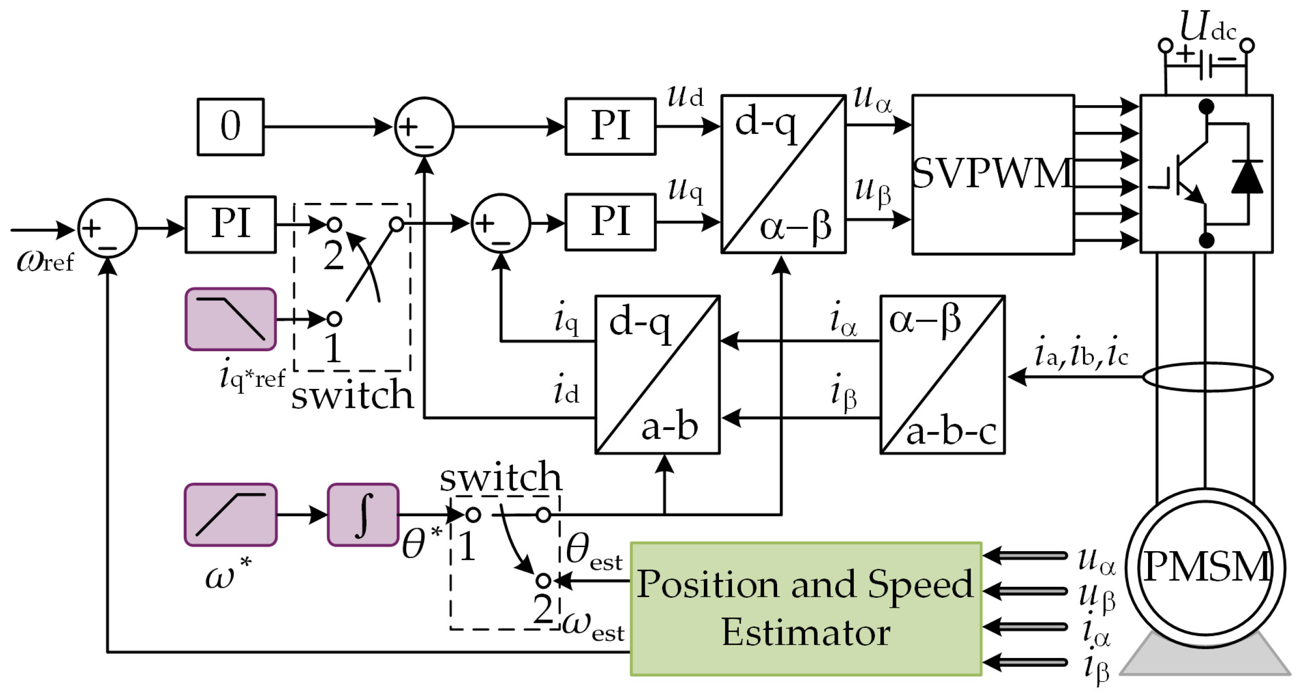
I-f control is a control strategy characterized by closed-loop current regulation and open-loop speed regulation. By regulating the amplitude and frequency of the stator current vector, a rotating magnetic field is established, thereby generating electromagnetic torque to drive the motor. As shown in Figure 1, when the switch in the dashed box is connected to position 1, the system operates in the I-f control mode, which consists of a frequency reference and a closed-loop current regulator. Specifically, the frequency reference determines the rotational speed of the current vector, while the current regulator ensures accurate tracking of the stator current amplitude reference.
The startup process under I-f control involves adjusting the amplitude and frequency of the current vector in stages to drive the motor from a standstill to an operating state that meets the criteria for sensorless closed-loop control. This process is generally divided into four stages. First is the rotor alignment stage, where a current vector in a fixed direction is applied to stabilize the rotor at a predetermined initial position. Subsequently, the acceleration stage begins, in which the frequency reference is gradually increased while maintaining a constant stator current amplitude to accelerate the rotor. When the speed reaches the preset switching speed, the system enters the constant-speed switching stage, during which the frequency reference remains constant while the current amplitude is progressively reduced to bring the operating state closer to closed-loop control. Finally, when the criteria for mode switching are met, the system switches from I-f control to sensorless closed-loop control, corresponding to the case where the switch in the dashed box of Figure 1 is connected to position 2.

2.2. Angle Error and Torque Self-Balancing Characteristic

In the I-f control process, since the actual rotor position is unknown, the coordinate transformation adopts virtual electrical angle θ*, which is obtained by integrating the frequency reference ω*, expressed as:
θ * = ω * d t
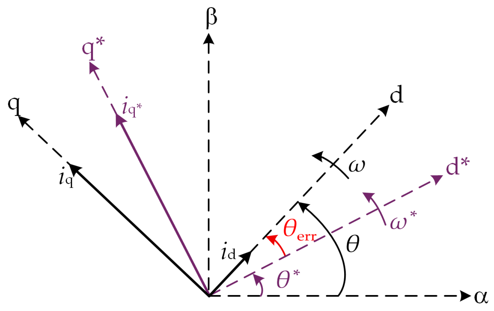
For the convenience of analysis, a virtual d*q* synchronous rotating coordinate system is established, as shown by the purple dashed lines in Figure 2.
Since θ* does not coincide with the actual electrical angle θ, an angle error θerr exists between the dq coordinate system and the d*q* coordinate system. The existence of θerr causes differences in the decomposed components of the same vector in the two coordinate systems. Taking the stator current vector as an example, as shown in Figure 2, the stator current is commanded along the q*-axis in the d*q* coordinate system, appearing only as the q*-axis component iq*. However, in the dq coordinate system, the stator current simultaneously contains both a d-axis component id and a q-axis component iq.
As shown in Figure 2, the space vector components in the d*q* coordinate system and the dq coordinate system satisfy the following relationship:
x d x q = cos θ err sin θ err sin θ err cos θ err x d * x q *
where x represents space vectors such as current and voltage; xd and xq are the components in the dq coordinate system; xd* and xq* are the components in the d*q* coordinate system; and the angle error θerr is given by:
θ err = θ θ *
The above relationship indicates that when θerr is non-zero, there are differences in the representations of the same space vector components in the two coordinate systems. To achieve a smooth switching process, θerr must converge to zero during the switching stage so that the state variables in the two coordinate systems approach consistency.
In I-f control, the current command is given along the q*-axis; i.e., id* = 0. By applying Equation (2) to the stator current vector, the following relationship can be obtained:
i d = i q * sin θ err
i q = i q * cos θ err
Equations (4) and (5) indicate that variations in θerr alter the projected components of the stator current vector on the d- and q-axes, which in turn cause changes in the electromagnetic torque. The electromagnetic torque generated by the HSPMSM during the I-f control process can be expressed as:
T e = 1.5 n p ψ f i q = 1.5 n p ψ f i q * cos θ err
where ψ f represents the permanent magnet flux linkage.
The mechanical equation of motion of the HSPMSM is expressed as:
J n p d ω d t = T e T L B ω n p
where J is the moment of inertia, np is the number of pole pairs, ω is the electrical angular velocity, TL is the load torque, Te is the electromagnetic torque, and B is the viscous friction coefficient of the motor.
The electromagnetic torque changes induced by θerr are fed back to the rotor operating state through the mechanical system, which in turn leads to further changes in θerr according to Equation (3). This process enables the system to exhibit a self-balancing characteristic between the electromagnetic torque and the angle error.
By defining the torque required to maintain motor rotation in Equation (6) as the motor’s demand torque Td, the following can be obtained:
T d = J n p d ω d t + T L + B ω n p
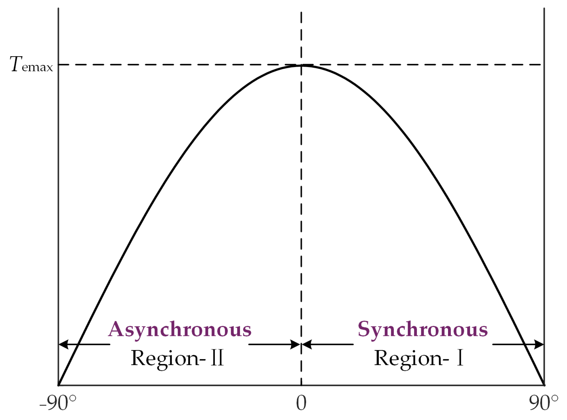
The I-f open-loop control process is essentially a continuous balancing process between Te and Td. The variation of Te with respect to θerr during the I-f control process is shown in Figure 3. During motor operation, θerr varies within the range of −90° to 90°. When θerr = 0°, the electromagnetic torque generated by the motor reaches its maximum value Temax:
T emax = 1.5 n p ψ f i q *
When Temax exactly balances Td, θerr converges to 0°. Based on whether θerr is greater than 0°, the system’s operating regions can be divided into Synchronous Region I and Asynchronous Region II. In Synchronous Region I, Te increases as θerr decreases; once Te and Td reach equilibrium, the system can maintain stable operation. Conversely, in Asynchronous Region II, Te decreases as θerr decreases, thereby breaking the torque balance between Te and Td, eventually leading to loss of synchronism and startup failure. Therefore, I-f control and its switching process must maintain system operation within Synchronous Region I to ensure that θerr possesses the self-balancing convergence characteristic.

2.3. Analysis of the Switching Dynamics of Traditional Switching Methods

In the constant-speed switching stage, ignoring the variations in load torque, the demand torque Td and the q-axis current component iqneed required to generate Td can be approximately regarded as constant. The electromagnetic torque expression in Equation (6) indicates that Te is jointly determined by θerr and iq*. To ensure the convergence of θerr, iq* must be adjusted during the switching stage. The torque balance relationship can be equivalently expressed as a matching relationship between iq* and iqneed, and the relationship between θerr and these two variables satisfies the following equation:
θ err = arccos i qneed i q *
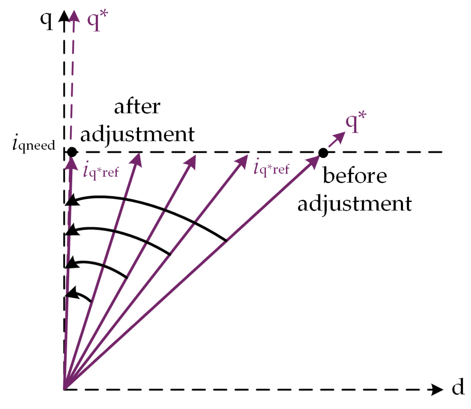
Equation (9) indicates that as iq* gradually decreases, θerr will decrease accordingly. When θerr approaches zero, the system meets the criteria for switching to sensorless closed-loop control. The schematic diagram of the process of completing the switch by reducing the q*-axis current is illustrated in Figure 4.
The traditional switching method reduces the q*-axis current at a constant rate, and the current reduction process can be expressed as:
i q * ref t = i q * t 0 k s t t 0
where ks is the rate of current reduction; t is the current time; t0 is the switching start time; iq*(t) is the q*-axis current reference at time t; and iq*(t0) is the q*-axis current at the start of the switching process.
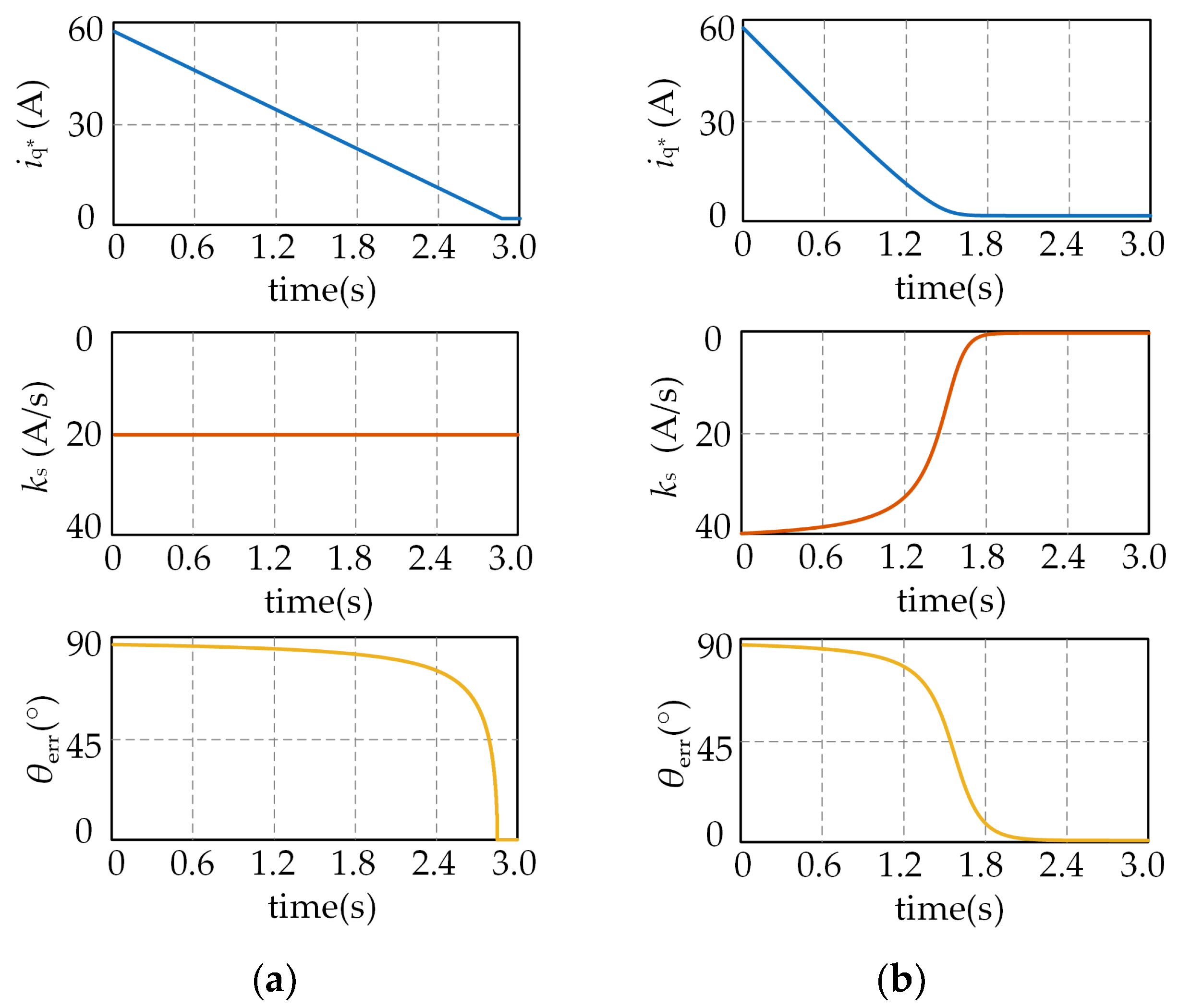
When the traditional switching method is adopted, the variation trends of iq*, ks, and θerr are illustrated in Figure 5a. As observed in the figure, the impact of iq* variations on θerr exhibits significant regional differences. In the early stage of the switching process when θerr is large, this impact is relatively weak; even a substantial change in current only causes a slight variation in the angle error. Conversely, in the later stage of the switching process when θerr approaches the boundary of the synchronous region, this impact is significantly enhanced, and even a small current change can lead to a pronounced variation in θerr. Once θerr drops below 0°, the system will cross the boundary and enter the unstable asynchronous region. Under light-load or no-load conditions, iqneed decreases. Equation (10) indicates that this further amplifies the sensitivity of θerr to iq* variations in the later stage, making it easier for θerr to rapidly cross into the asynchronous region.
Furthermore, the response of the mechanical system to torque variations is slower than that of the current loop regulation. Consequently, θerr exhibits a dynamic lag relative to the variations in iq*, and the convergence of θerr often lags behind the regulation process of iq*. If the current reduces too rapidly in the later stage of the switching process, iq* may have already dropped close to iqneed before θerr has converged. By the time θerr finally converges, iq* may have reached an even lower level, causing the system operating point to cross the synchronous region boundary and enter the asynchronous region, thereby triggering loss of synchronism. Moreover, the mismatch between the convergence process of θerr and the regulation of iq*, caused by the mechanical lag, induces an instantaneous reconfiguration of components such as current and voltage at switching. This results in current surge and speed fluctuation, which adversely affect switching stability.

3. Proposed Adaptive Switching Method Based on the Cosine of the Angle Error

3.1. Design of the Adaptive Attenuation Factor

Under the condition that the total current reduction required to complete the switching remains constant, the switching time is primarily determined by the rate of current reduction ks. A larger ks leads to a shorter switching time; however, an excessively rapid current reduction will cause the angle error to vary too quickly during the later stage of the switching process, thereby increasing the risk of crossing the boundary into the asynchronous region. Conversely, a smaller rate of current reduction can ensure stability in the later stage, but it prolongs the overall switching time.
The design of the rate of current reduction during the switching stage should minimize the switching time under the constraints of the synchronous region while ensuring stability in the later stage of the switching process. Considering the variation trend of the angle error, a larger rate of current reduction should be permitted in the early stage of the switching process when θerr is large to accelerate the process. In the later stage of the switching process when θerr is small, the rate of current reduction should be as small as possible and its variation should remain gradual. This avoids rapid variations in θerr, provides sufficient adjustment time for the mechanical lag, and reduces the risk of crossing into the asynchronous region during the later stage of the switching process.
To regulate ks according to θerr, this study introduces an adaptive attenuation factor related to the cosine of the angle error to perform online adjustment of the baseline rate of current reduction, ks0. The rate of current reduction is designed as follows:
k s = k s 0 α θ err
where α(θerr) is the dimensionless adaptive attenuation factor, expressed as:
α θ err = 1 cos θ err
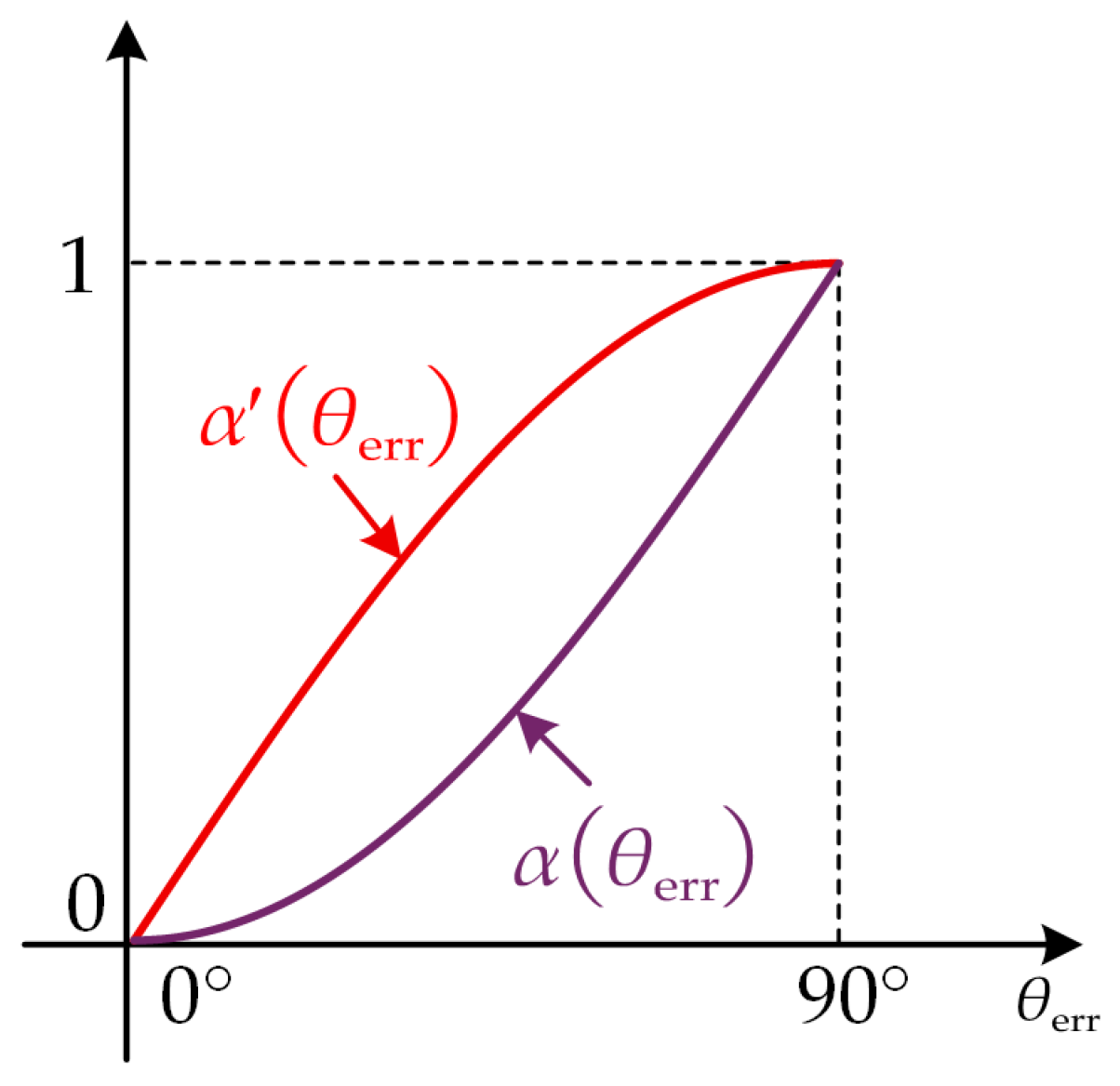
Figure 6 illustrates the variation trends of α(θerr) and its derivative α′(θerr) = sin(θerr) within the range of 0° to 90°. By adopting this attenuation factor, the rate of current reduction can be continuously adjusted with θerr. When θerr is large, α(θerr) is close to 1, allowing a high rate of current reduction in the early stage of the switching process to shorten the switching time. As the angle error decreases, α(θerr) gradually reduces, naturally slowing down the current reduction process. In the later stage of the switching process, when θerr approaches the synchronous region boundary of 0°, α(θerr) approaches 0, thereby mitigating the rapid variation in the angle error. Meanwhile, the fact that α′(θerr) also approaches 0 as θerr nears 0° indicates that α(θerr) varies slowly. This provides sufficient adjustment time for the mechanical lag and alleviates the mismatch between θerr convergence and iq* regulation.
Meanwhile, during the switching process, θerr can directly reflect the synchronization state of the system. When operating conditions change, the torque balance relationship adjusts accordingly, and θerr varies synchronously. By introducing θerr into the adaptive attenuation factor, the rate of current reduction can be adjusted online according to the synchronization state. This allows the current regulation process to respond promptly to variations in operating conditions and adapt accordingly, thereby reducing the risk of crossing the boundary caused by disturbances and enhancing the disturbance rejection capability and robustness during the switching process.

3.2. Generation of the Current Reference

Before the establishment of sensorless closed-loop control, the angle error θerr can be calculated as:
θ err = θ est θ *
where θest is the electrical angle estimated by the sensorless observer.
The reduction process of the q*-axis current reference is expressed as:
i q * ref t = i q * t 0 k s 0 1 cos θ err d t
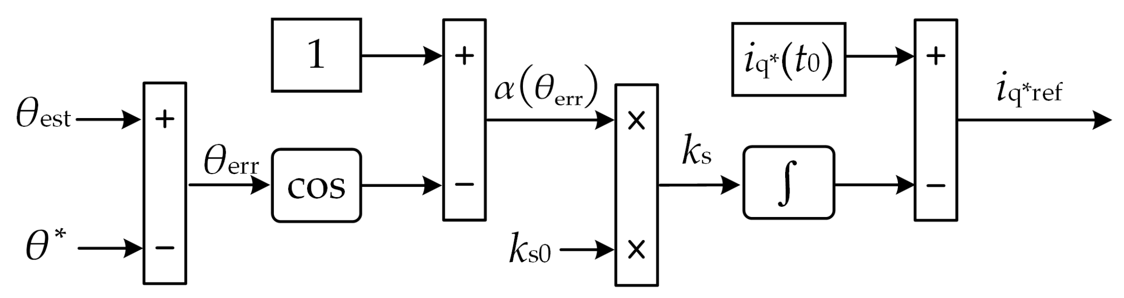
Figure 7 illustrates the block diagram of q*-axis current reference generation in the proposed switching method. As shown, the proposed method takes θerr as the input to generate the adaptive attenuation factor α(θerr), which is then multiplied by the baseline rate of current reduction ks0 to obtain the instantaneous rate of current reduction ks. Subsequently, ks is integrated and subtracted from the initial value of the q*-axis current at the start of the switch to obtain the q*-axis current reference.
Figure 5b illustrates the variation processes of iq*, ks, and θerr when the proposed method is adopted. As shown in the figure, ks varies continuously throughout the switching process. It remains at a relatively large value during the early stage, allowing a faster current reduction, and gradually decreases as θerr decreases. Furthermore, as θerr approaches 0°, ks tends towards 0 and varies slowly, which enables a smoother convergence of θerr. This effectively mitigates the rapid variation of θerr in the later stage of the switching process and reduces the risk of crossing the boundary into the asynchronous region.

3.3. Stability Analysis and Parameter Tuning

3.3.1. Small-Signal Stability Analysis

In the I-f control process, a frequency correction method based on active power fluctuation is typically introduced to enhance system damping and suppress low-frequency oscillations. According to [20,21], by linearizing the system around the steady-state operating point during the constant-speed switching stage, the transfer function from the q*-axis current perturbation to the angle error can be obtained as:
Δ θ err s Δ i q * s = n p K I J s 2 + B eq s + K eq
where ∆θerr represents the small-signal perturbation around the steady-state angle error θerr0 (i.e., ∆θerr = θerrθerr0), and other small-signal terms are defined similarly. Kp is the active power feedback gain, the parameters KI and Kθ can be calculated by Equation (16), and the definitions of Beq and Keq are given in Equation (17).
K θ = T e θ err θ err 0 = 1.5 n p ψ f i q * sin θ err 0 K I = T e i q * θ err 0 = 1.5 n p ψ f cos θ err 0
B eq = B + ω 0 K p K θ J n p K eq = n p K θ 1 + K p 2 B ω 0 n p 2 + T L 0 n p
Linearizing Equation (15) around the steady-state operating point θerr0 yields:
d Δ i q * d t = k s 0 sin θ err 0 Δ θ err 0
Transforming Equation (19) into the s-domain yields:
Δ i q * s = k s 0 sin θ err 0 s Δ θ err s
By substituting Equation (20) into Equation (16), the closed-loop characteristic equation of the system can be obtained as:
J s 3 + B eq s 2 + K eq s + n p K I k s 0 sin θ err 0 = 0
Within the synchronous region (0° < θerr < 90°), we have sin(θerr0) > 0, Beq > 0, and Keq > 0. By applying the Routh–Hurwitz criterion to Equation (20), the key inequality required to ensure system stability is obtained as:
B eq K eq > J n p K I k s 0 sin θ err 0
The stability range of ks0 can be obtained from Equation (21) as:
k s 0 < B eq K eq J n p K I sin θ err 0 = B eq i q 0 * 1 + K p 2 B ω 0 n p 2 + T L 0 n p J cos θ err 0
When ks0 satisfies the constraint in Equation (22), it is ensured that ks remains within the allowable stability limits, thereby ensuring the overall stability of the system.

3.3.2. Parameter Tuning

According to Equation (23), the baseline rate of current reduction ks0 is jointly constrained by the mechanical inertia J and Beq. For the convenience of tuning, a conservative lower bound for the baseline rate of current reduction ks0 can be calculated under the limit condition where θerr0 is 0°, as expressed in the following equation:
k s 0 < i q 0 * B 1 + K p 2 B ω 0 + T L 0 J
Since the angle error threshold for mode switching, θth, is greater than 0°, the actual permissible lower bound of ks0 is greater than the conservative value given in Equation (24). In this paper, θth is set to 5°. The minimum baseline rate of current reduction ks0 obtained through experimental testing is 210 A/s, while the conservative lower bound calculated by Equation (24) is approximately 190 A/s.
During parameter tuning, ks0 is used to balance the switching speed and stability constraints. The tuning should be constrained to ensure that the angle error does not cross the boundary of the synchronous region. Under the premise of satisfying stability, ks0 should be as large as possible and adjusted empirically based on the system’s moment of inertia and the target switching time.

4. Experimental Results and Analysis

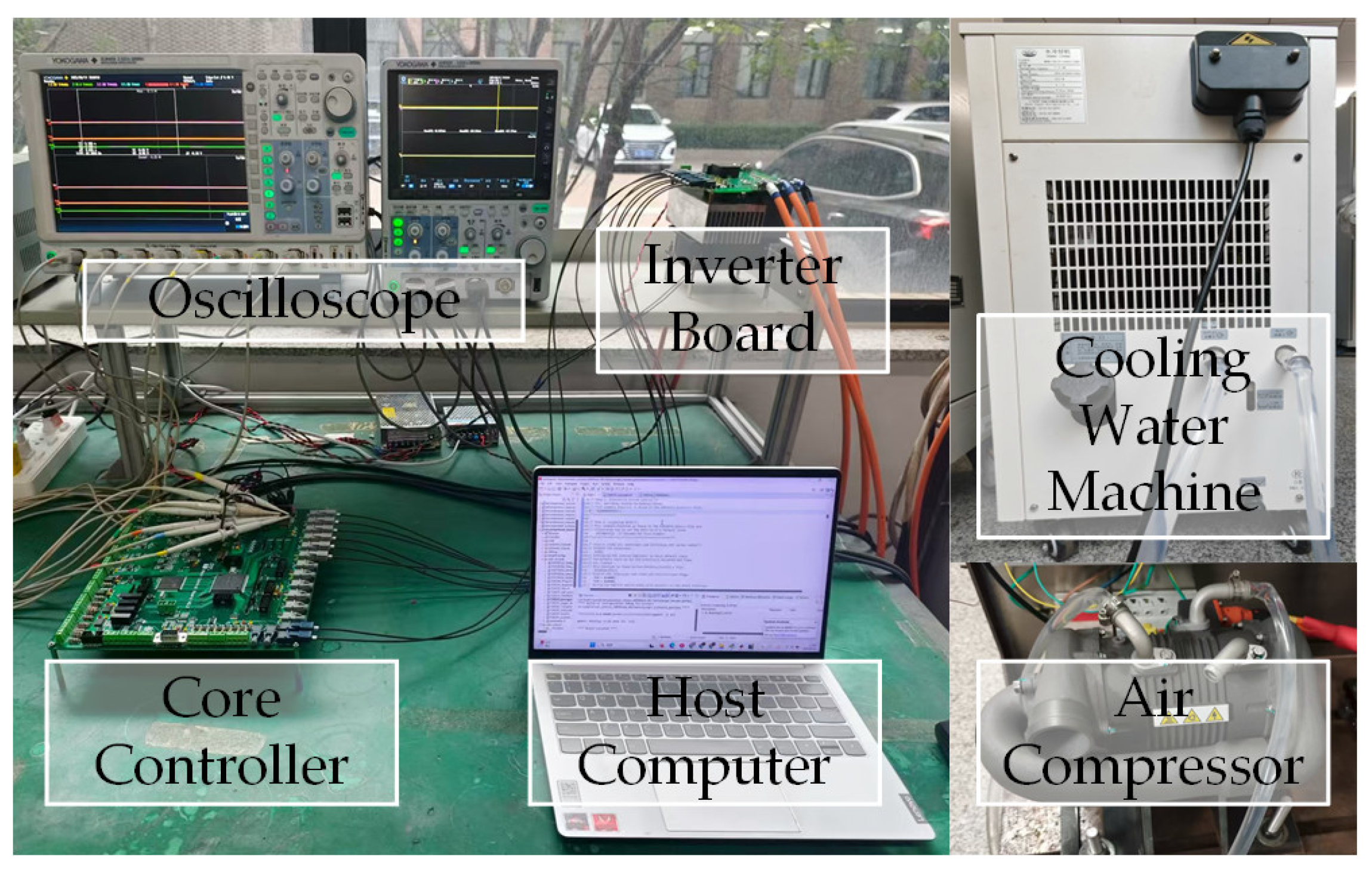
To verify the effectiveness of the proposed adaptive switching method, experimental validation was conducted on the high-speed air compressor experimental platform shown in Figure 8. The experimental motor is an HSPMSM, and its main parameters are listed in Table 1. The motor is equipped with air bearing, and the floating speed of the air bearing is 20,000 r/min. Therefore, the continuous operating speed of the motor must be maintained above this threshold. The control system utilizes a DSP (TMS320F28335) and an FPGA (EP1C6Q240C8) as the central control units. SiC devices are employed for the inverter power stage. Both the control frequency and the sampling frequency are 40 kHz.
In the experiments, the motor accelerates to the switching speed with an acceleration of 60,000 r/min/s during the acceleration stage, followed by the execution of the switching process. The switching is determined to be complete when the angle error θerr remains below the predefined threshold θth = 5° for 50 consecutive control cycles. At medium and high speeds, a sliding mode observer combined with a phase-locked loop structure [24,25,26] is employed to estimate the rotor position and speed.

4.1. Comparison of Minimum Switching Time

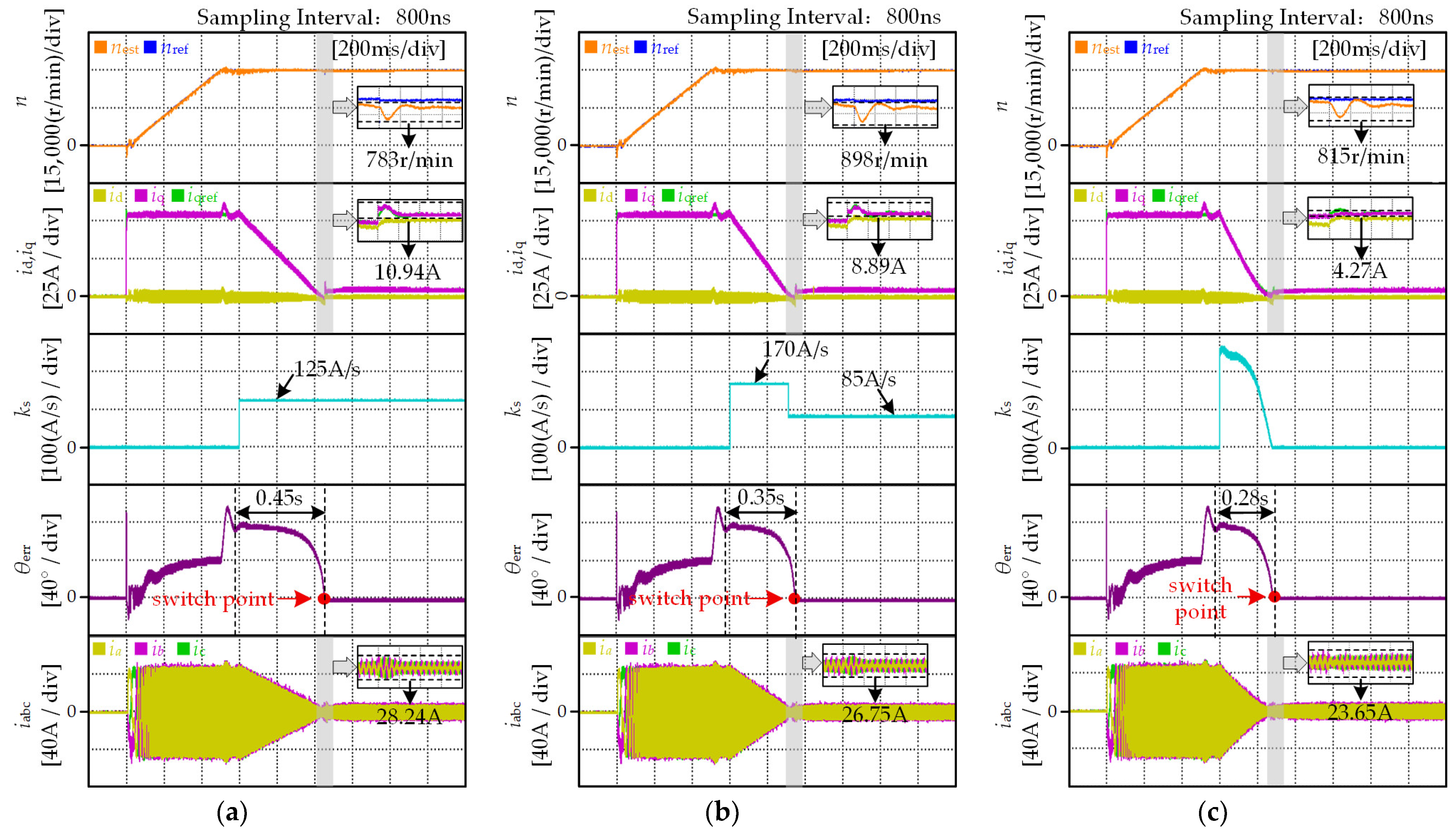
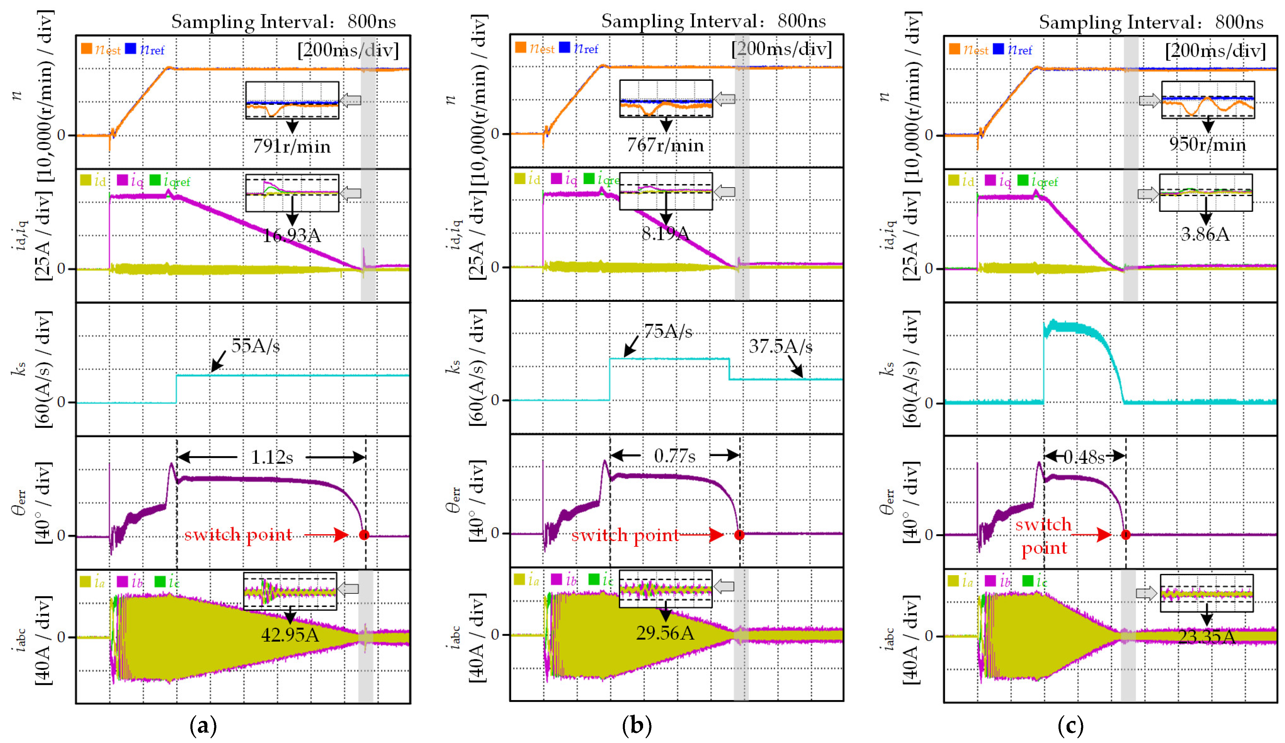
To ensure that the system does not lose synchronism, the minimum switching times achievable by different methods were compared. In the experiments, the constant-rate switching method in [12], the piecewise-rate switching method in [13], and the proposed adaptive switching method were implemented. By gradually increasing the rate of current reduction, the shortest switching time achieved immediately before loss of synchronism was defined as the minimum switching time for each method. The results are summarized in Table 2. The startup processes under the minimum switching times for each method at 20,000 r/min and 30,000 r/min are shown in Figure 9 and Figure 10, respectively. Unless otherwise stated, the gray stripes in the following figures indicate the regions enlarged in the inner subplots, and the black dashed lines in the inner subplots indicate the upper and lower envelopes of the waveforms.
As shown in Table 2, at a switching speed of 20,000 r/min, the minimum switching time of the proposed method is 0.48 s, while those of the constant-rate and piecewise-rate methods are 1.12 s and 0.77 s, respectively. Compared with these two methods, the proposed method achieves time reductions of 57.14% and 37.66%. At 30,000 r/min, the minimum switching time of the proposed method is 0.28 s, representing reductions of 37.77% and 20.00% compared to the 0.45 s of the constant-rate method and 0.35 s of the piecewise-rate method, respectively. Furthermore, during the startup process under the minimum switching time, the current surge at switching for the proposed method remains at a low level; the q-axis current fluctuation is 3.86 A at 20,000 r/min and 4.27 A at 30,000 r/min. This indicates that while satisfying system stability constraints, the proposed method effectively suppresses switching transient oscillations and mitigates current surges.
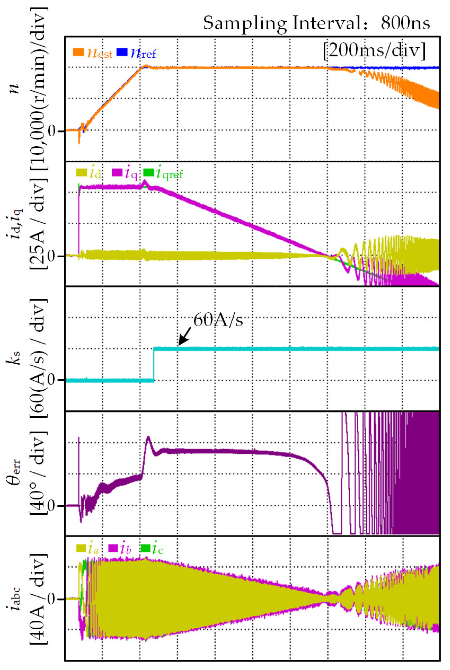
The process of losing synchronism for the constant-rate switching method is shown in Figure 11. It can be observed that with a large rate of current reduction, θerr varies rapidly and crosses the boundary of synchronous region in the later stage of the switching process. Consequently, the torque balance is disrupted, leading to loss of synchronism and startup failure.

4.2. Comparison of Switching Process Stability Under Identical Switching Times

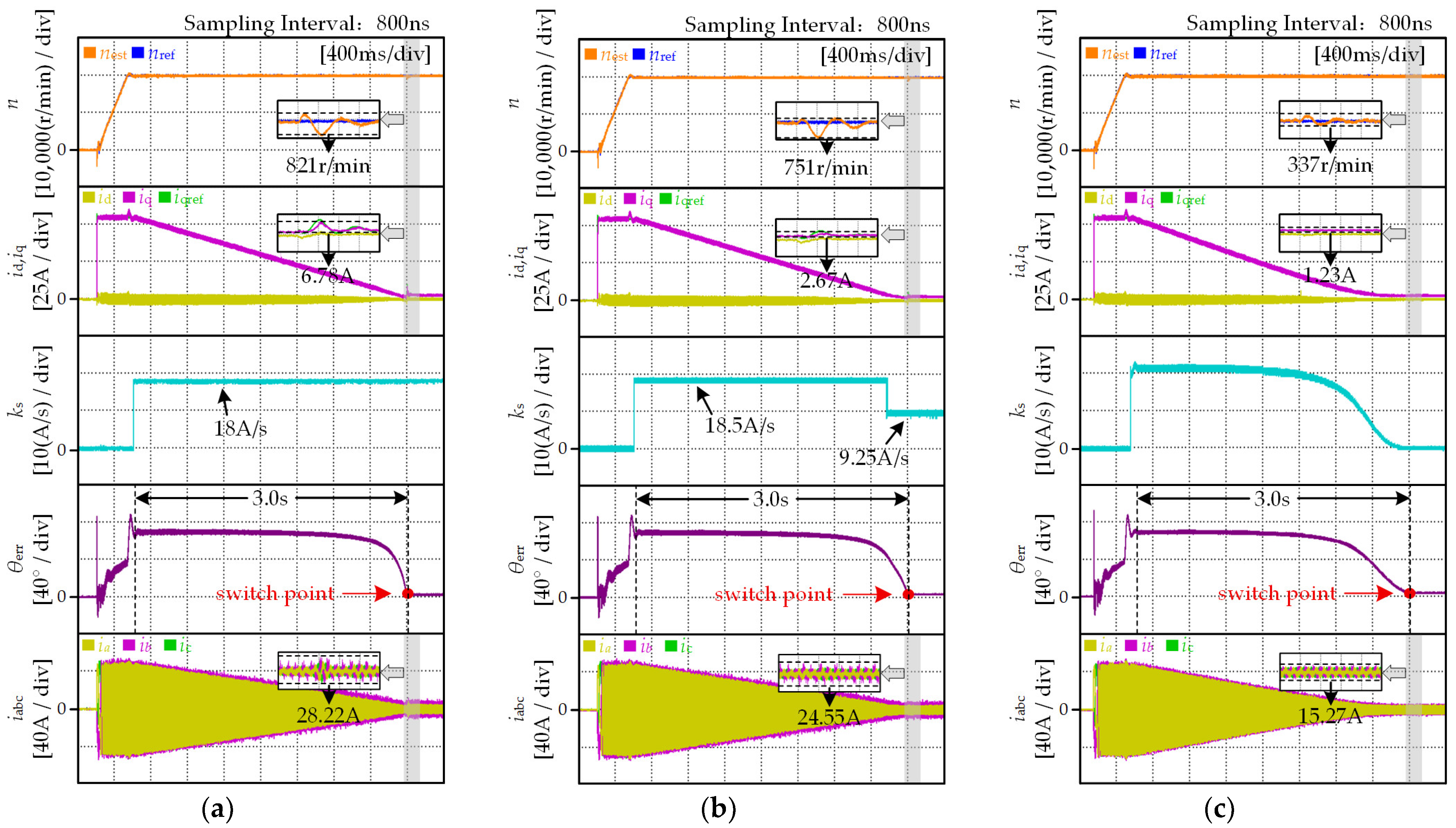
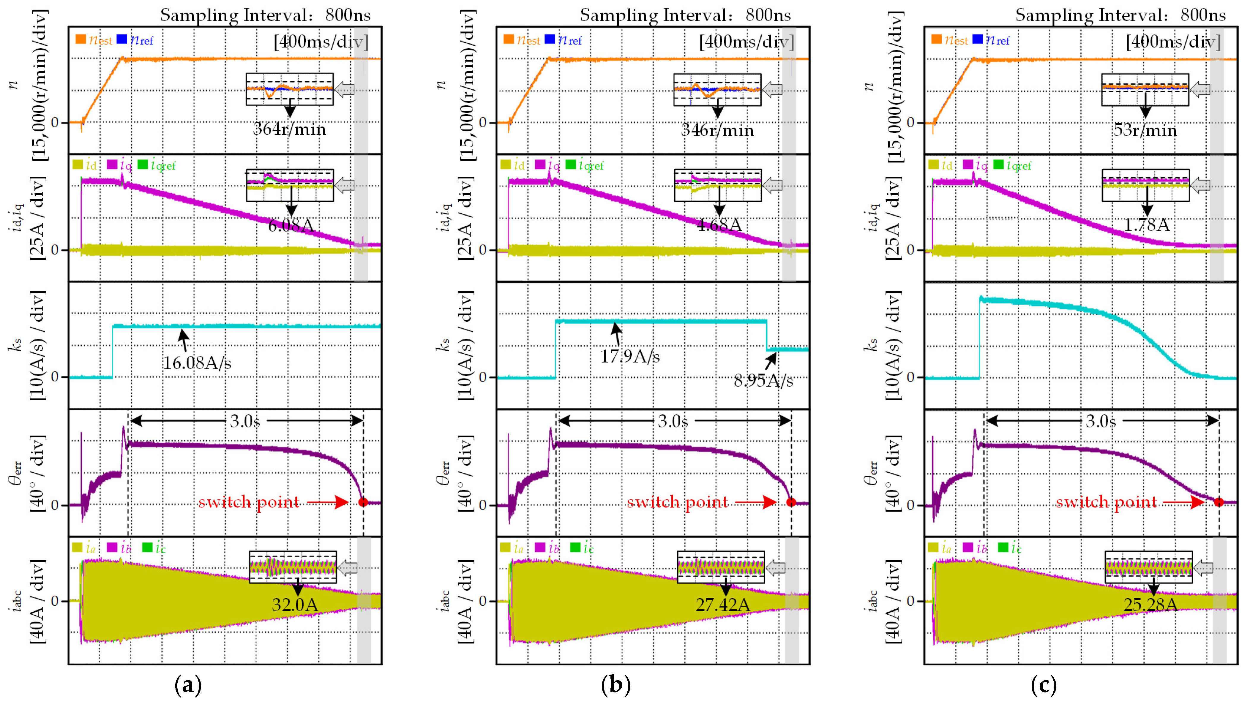
Under the condition of identical switching times, the switching stability of different switching methods was compared under experimental conditions. In the experiments, the switching times were set to 3.0 s through parameter tuning. The startup processes at switching speeds of 20,000 r/min and 30,000 r/min are shown in Figure 12 and Figure 13, respectively, and their main performance indicators are summarized in Table 3.
As shown in Table 3, there are distinct differences in the switching stability among the different methods. At a switching speed of 20,000 r/min, the speed fluctuation amplitude with the proposed switching method is 337 r/min, which is significantly lower than the 821 r/min of the constant-rate switching method and the 751 r/min of the piecewise-rate switching method. Simultaneously, the q-axis current fluctuation amplitude is reduced to 1.23 A, and the peak-to-peak value of the three-phase current is also markedly decreased. At 30,000 r/min, the speed fluctuation amplitude of the proposed method further decreases to 53 r/min, and the q-axis current fluctuation is 1.78 A, both of which are superior to those of the other two methods.
The above results indicate that the traditional constant-rate switching method exhibits the most pronounced speed and current fluctuations after switching is completed. Although the piecewise-rate switching method can reduce the impact to some extent, significant speed and current fluctuations still persist. In contrast, the proposed switching method effectively suppresses these fluctuations at both switching speeds, achieving a smoother switching process.

4.3. Robustness Verification Under Varying Operating Conditions

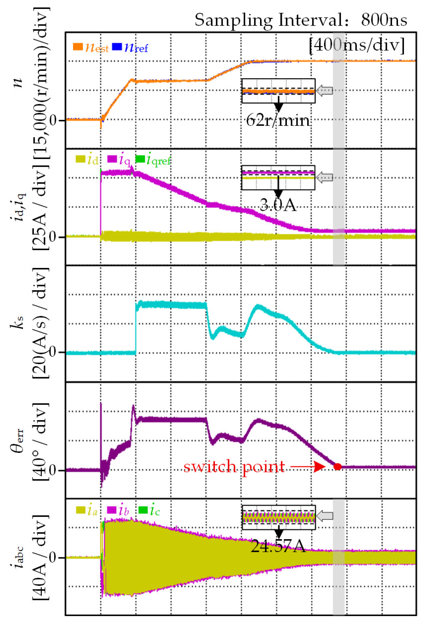
To verify the robustness of the proposed switching method under varying operating conditions, a case involving speed variations during the switching process was introduced. Since the load torque of the air compressor is speed-dependent, a change in speed inherently represents a change in load torque. In the experiment, the motor accelerated from 20,000 r/min to 30,000 r/min at an acceleration of 20,000 r/min/s at 1.2 s during the switching process. The startup process is shown in Figure 14.
As shown in Figure 14, the speed variation leads to a realignment of the torque balance, causing θerr to change accordingly. Consequently, the rate of current reduction is adjusted online based on θerr: during acceleration, θerr decreases, and the rate of current reduction decreases accordingly; after acceleration is completed, θerr increases, and the rate of current reduction increases as well. Throughout the entire switching process, the speed and current remain continuous and smooth without obvious abnormal oscillations, which verifies the robustness of the proposed method under varying operating conditions.

5. Conclusions

This study proposes an adaptive switching method based on the cosine of the angle error for sensorless startup of HSPMSMs using I-f control. Firstly, the torque self-balancing characteristic of the angle error and the instability mechanism of traditional switching methods are analyzed. Subsequently, the cosine of the angle error is introduced into the current regulation process to achieve online adjustment of the rate of current reduction and a small-signal stability analysis is performed to guide parameter design. The proposed method features a simple structure and requires only a few tuning parameters. Finally, the proposed method is verified on a high-speed air compressor experimental platform. The experimental results show that, under an identical switching time of 3.0 s, the speed fluctuation is reduced to 337 r/min and 53 r/min, and the q-axis current fluctuation is reduced to 1.23 A and 1.78 A at 20,000 r/min and 30,000 r/min, respectively. In addition, the proposed method achieves minimum switching times of 0.48 s and 0.28 s at switching speeds of 20,000 r/min and 30,000 r/min, respectively.
Future work will focus on extending the proposed method beyond the constant-speed switching condition. In particular, more attention will be given to achieving fast and smooth switching during the acceleration process, so that the switching stage can be completed earlier without waiting for speed stabilization. This is expected to further shorten the overall startup time and improve the dynamic performance of HSPMSM sensorless startup.


Author Contributions

Conceptualization, W.C.; Funding acquisition, W.C., X.L. and S.X.; Investigation, S.Z., X.L. and S.X.; Methodology, W.C. and S.Z.; Project administration, W.C. and Z.W.; Resources, X.L. and Z.X.; Software, S.Z.; Supervision, W.C.; Validation, S.Z.; Writing—original draft, S.Z.; Writing—review and editing, W.C., Z.W. and Z.X. All authors have read and agreed to the published version of the manuscript.

Funding

This research was funded by the Zhejiang Province Pioneer Project (Grant No. 2024C01014), the Joint Fund Key Project of the National Natural Science Foundation of China (Grant No. U23A20643), the National Natural Science Foundation of China (Grant No. 52477060), and the Basic Scientific Research Institute Stability Support Project (Grant No. WDZC-2023-ZNKZ-01).

Data Availability Statement

Data is contained within the article.

Conflicts of Interest

The authors declare no conflicts of interest. The funders had no role in the design of the study; in the collection, analyses, or interpretation of data; in the writing of the manuscript; or in the decision to publish the results.

References

  1. Zhang, Y.; Xu, W.; Wang, J. A rapid sensorless startup method with instantaneous control mode switching for high-speed vane-motor based on hybrid speed-position-current tracking controller. IEEE Trans. Power Electron. 2024, 39, 6125–6135. [Google Scholar] [CrossRef] [Scilit]
  2. Niedermayr, P.; Alberti, L.; Bolognani, S.; Abl, R. Implementation and experimental validation of ultrahigh-speed PMSM sensorless control by means of extended Kalman filter. IEEE J. Emerg. Sel. Top. Power Electron. 2022, 10, 3337–3344. [Google Scholar] [CrossRef] [Scilit]
  3. Upadhyaya, A.; Nair, A.M.; Petersen, N.P.; Severson, E.L. Back-EMF based self-sensing drive for ultra-high-speed surface mount PMSM. IEEE Trans. Ind. Appl. 2025, 61, 9281–9294. [Google Scholar] [CrossRef] [Scilit]
  4. Zuo, Y.; Lai, C.; Iyer, K.L.V. A review of sliding mode observer based sensorless control methods for PMSM drive. IEEE Trans. Power Electron. 2023, 38, 11352–11367. [Google Scholar] [CrossRef] [Scilit]
  5. Ye, M.; Cao, Y.; Chen, W.; Shi, T.; Xia, C. Full-speed-range sensorless control of high-speed permanent magnet synchronous motor based on the prediction methodology. IEEE Trans. Power Electron. 2025, 40, 3405–3418. [Google Scholar] [CrossRef] [Scilit]
  6. Chen, S.; Ding, W.; Wu, X.; Huo, L.; Hu, R.; Shi, S. Sensorless control of IPMSM drives using high-frequency pulse voltage injection with random pulse sequence for audible noise reduction. IEEE Trans. Power Electron. 2023, 38, 9395–9408. [Google Scholar] [CrossRef] [Scilit]
  7. Rangarajan, S.; Agarwal, V. Novel active damping scheme for stable and high performance v/f controlled permanent magnet synchronous motor driven passenger elevator system. IEEE Trans. Ind. Electron. 2025, 72, 5636–5645. [Google Scholar] [CrossRef] [Scilit]
  8. Tang, Q.; Chen, D.; He, X. Integration of improved flux linkage observer and I-f starting method for wide-speed-range sensorless SPMSM drives. IEEE Trans. Power Electron. 2020, 35, 8374–8383. [Google Scholar] [CrossRef] [Scilit]
  9. Gong, J.; Zhang, J.; Wang, X.; Ky Nguyen, N. A robust full-speed position-sensorless control for a nonsinusoidal seven-phase permanent magnet machine. IEEE Trans. Transp. Electrif. 2025, 11, 9048–9059. [Google Scholar] [CrossRef] [Scilit]
  10. Kim, H.; Song, J.; Lee, K. Q-MRAS based I-F startup for model predictive current controlled sensorless SPMSM drive. IEEE Trans. Ind. Appl. 2025, 61, 9394–9403. [Google Scholar] [CrossRef] [Scilit]
  11. Nair, S.V.; Hatua, K.; Prasad, N.V.P.R.D.; Reddy, D.K. A quick I-f starting of PMSM drive with pole slipping prevention and reduced speed oscillations. IEEE Trans. Ind. Electron. 2021, 68, 6650–6661. [Google Scholar] [CrossRef] [Scilit]
  12. Liu, P.; Liu, D.; Shen, Y.; Liu, A.; Yang, X.; Zhao, J. Full speed range position-sensorless compound control scheme for PMSMs. J. Power Electron. 2022, 22, 1302–1312. [Google Scholar] [CrossRef] [Scilit]
  13. Wang, Q.; Wang, S.; Chen, C. A novel full-speed sensorless control strategy based on electric vehicle PMSM. In Proceedings of the 21st International Conference on Electrical Machines and Systems, Jeju, Republic of Korea, 7–10 October 2018; pp. 1680–1685. [Google Scholar] [CrossRef] [Scilit]
  14. Wang, C.; Zhang, W.; Yu, G.; Wang, W.; Xu, Y. Position sensorless startup scheme for PMSM drives with single current sensor. In Proceedings of the IEEE Transportation Electrification Conference and Expo, Asia-Pacific, Harbin, China, 28–31 October 2022; pp. 1–6. [Google Scholar] [CrossRef] [Scilit]
  15. Xu, Y.; Lin, C.; Xing, J.; Zeng, Q.; Sun, J. I-f starting rapid and smooth transition method of full-speed sensorless control for low current harmonic ultra-high-speed PMSM. In Proceedings of the IEEE Applied Power Electronics Conference and Exposition, Houston, TX, USA, 20–24 March 2022; pp. 1820–1826. [Google Scholar] [CrossRef] [Scilit]
  16. Wang, M.; Xu, Y.; Zou, J.; Lan, H. An optimized I-f startup method for BEMF-based sensorless control of SPMSM. In Proceedings of the IEEE Transportation Electrification Conference and Expo, Asia-Pacific, Harbin, China, 7–10 August 2017; pp. 1–6. [Google Scholar] [CrossRef] [Scilit]
  17. Li, H.; Zhang, X.; Liu, S.; Xu, C. Hybrid sensorless control based on I/F and sliding mode observer using current nonlinear regulation for PMSM drives. In Proceedings of the 22nd International Conference on Electrical Machines and Systems, Harbin, China, 11–14 August 2019; pp. 1–5. [Google Scholar] [CrossRef] [Scilit]
  18. Li, Z.; Wang, S. A novel switching method for all-speed sensorless control strategy based on aviation motor. In Proceedings of the 2021 24th International Conference on Electrical Machines and Systems (ICEMS), Gyeongju, Republic of Korea, 31 October–3 November 2021; pp. 147–152. [Google Scholar] [CrossRef] [Scilit]
  19. Zhang, Z.; Guo, H.; Liu, Y.; Zhang, Q.; Zhu, P.; Iqbal, R. An improved sensorless control strategy of ship IPMSM at full speed range. IEEE Access 2019, 7, 178652–178661. [Google Scholar] [CrossRef] [Scilit]
  20. Wang, L.; Zhang, Y.; Zhao, L.; Chen, G. An improved 3-step startup method based on sensorless vector control of PMSM. In Proceedings of the IEEE PES Asia-Pacific Power and Energy Engineering Conference, Macao, China, 1–4 December 2019; pp. 1–5. [Google Scholar] [CrossRef] [Scilit]
  21. Chen, D.; Lu, K.; Wang, D.; Hinkkanen, M. I-F control with zero Daxis current operation for surface-mounted permanent magnet synchronous machine drives. IEEE Trans. Power Electron. 2023, 38, 7504–7513. [Google Scholar] [CrossRef] [Scilit]
  22. Song, Z.; Yao, W.; Lee, K.; Li, W. An efficient and robust I-f control of sensorless IPMSM with large startup torque based on current vector angle controller. IEEE Trans. Power Electron. 2022, 37, 15308–15321. [Google Scholar] [CrossRef] [Scilit]
  23. Ning, B.; Zhao, Y.; Cheng, S. An Improved Sensorless Hybrid Control Method of Permanent Magnet Synchronous Motor Based on I/F Startup. Sensors 2023, 23, 635. [Google Scholar] [CrossRef] [Scilit] [PubMed]
  24. Shabani, A.; Mirzaie, M.; Khamesipour, M.; Khaburi, D.A. A modified adaptive complex coefficient filter based on sigmoid function for sensorless control of SPM motors with an I-F startup strategy. In Proceedings of the 2025 16th Power Electronics, Drive Systems, and Technologies Conference, Tabriz, Iran, 4–6 February 2025; pp. 1–6. [Google Scholar] [CrossRef] [Scilit]
  25. Yang, H.; Xu, A.; Zhang, Y.; Chai, X. Error analysis and design of sliding-mode-observer-based sensorless PMSM drives under a low sampling ratio. IEEE Trans. Power Electron. 2024, 39, 7783–7792. [Google Scholar] [CrossRef] [Scilit]
  26. Liu, G.; Zhang, H.; Song, X. Position-estimation deviation-suppression technology of PMSM combining phase self-compensation SMO and feed-forward PLL. IEEE J. Emerg. Sel. Top. Power Electron. 2021, 9, 335–344. [Google Scholar] [CrossRef] [Scilit]
Figure 1. Block diagram of I-f control.
Energies 19 02140 g001
Figure 2. Schematic diagram of the dq and d*q* coordinate systems.
Energies 19 02140 g002
Figure 3. Variation in electromagnetic torque with respect to angle error in I-f control.
Energies 19 02140 g003
Figure 4. Schematic diagram of completing the switching by reducing the q*-axis current.
Energies 19 02140 g004
Figure 5. Variation processes of q*-axis current iq*, rate of current reduction ks, and angle error θerr under different switching methods: (a) Traditional method; (b) Proposed method.
Energies 19 02140 g005
Figure 6. Variation in α(θerr) and α′(θerr) within the range of 0° to 90°.
Energies 19 02140 g006
Figure 7. Block diagram of q*-axis current reference generation in the proposed switching method.
Energies 19 02140 g007
Figure 8. Photographs of the high-speed air compressor experimental platform.
Energies 19 02140 g008
Figure 9. Startup processes under minimum switching times at a switching speed of 20,000 r/min: (a) Constant-rate switching method; (b) Piecewise-rate switching method; (c) Proposed adaptive switching method.
Energies 19 02140 g009
Figure 10. Startup processes under minimum switching times at a switching speed of 30,000 r/min: (a) Constant-rate switching method; (b) Piecewise-rate switching method; (c) Proposed adaptive switching method.
Energies 19 02140 g010
Figure 11. Experimental waveforms of the process of loss of synchronism with the constant-rate switching method.
Energies 19 02140 g011
Figure 12. Switching process under identical switching time at 20,000 r/min with different methods: (a) Constant-rate switching method; (b) Piecewise-rate switching method; (c) Proposed adaptive switching method.
Energies 19 02140 g012
Figure 13. Switching process under identical switching time at 30,000 r/min with different methods: (a) Constant-rate switching method; (b) Piecewise-rate switching method; (c) Proposed adaptive switching method.
Energies 19 02140 g013
Figure 14. Switching process of the proposed switching method under varying speed conditions.
Energies 19 02140 g014
Table 1. Main parameters of the experimental motor.
ParameterValue
Rated Power10.8 kW
Rated Speed110,000 r/min
Rated current (RMS)34.6 A
Minimum Speed20,000 r/min
DC bus voltage500 V
Pole pairs1
Stator resistance33.95 mΩ
d-/q-axis inductance96.5 μH
Motor inertia0.00009843 kg·m2
Flux linkage0.01666 Wb
Table 2. Comparison of minimum switching time for different methods at various switching speeds.
Switching Speed
(r/min)
Minimum Switching Time (s)
Constant-Rate Switching MethodPiecewise-Rate Switching MethodProposed Adaptive Switching Method
20,0001.120.770.48
30,0000.450.350.28
Table 3. Comparison of fluctuation indicators under identical switching times.
Switching Speed (r/min)Switching MethodSpeed Fluctuation (r/min)q-Axis Current
Fluctuation (A)
Three-Phase
Peak-to-Peak Current (A)
20,000constant-rate switching8216.7828.22
piecewise-rate switching7512.6724.55
proposed adaptive switching3371.2315.27
30,000constant-rate switching3646.0832.0
piecewise-rate switching3464.6827.42
proposed adaptive switching531.7825.28
Disclaimer/Publisher’s Note: The statements, opinions and data contained in all publications are solely those of the individual author(s) and contributor(s) and not of MDPI and/or the editor(s). MDPI and/or the editor(s) disclaim responsibility for any injury to people or property resulting from any ideas, methods, instructions or products referred to in the content.