Article

Comparison of Analytical and Numerical Methods for Predicting the Shell-Side Heat Transfer Coefficient in Heat Exchanger with Segmental Baffles

Institute of Energy, Gdańsk University of Technology, Narutowicza 11/12, 80-233 Gdańsk, Poland
*
Author to whom correspondence should be addressed.
Energies 2026, 19(9), 2114; https://doi.org/10.3390/en19092114
Submission received: 17 March 2026 / Revised: 9 April 2026 / Accepted: 23 April 2026 / Published: 28 April 2026

Abstract

This study reports the calculated values results of the shell-side heat transfer coefficient for a shell-and-tube heat exchanger with an inner shell diameter of 200 mm and a length of 518 mm, containing 85 tubes arranged in a staggered layout. Shell-side cross-flow was generated by nine standard segmental baffles with a 25% baffle cut and a baffle pitch of 48 mm. In particular, the effect of 13 combinations of shell-to-baffle and baffle-to-tube gaps on the heat transfer coefficient was investigated. Moreover, the influence of sealing strips and tube bundle diameter on the heat transfer coefficient was also examined. The calculations were carried out using three different approaches, namely the Gaddis-Gnielinski method, the extended Bell-Delaware method, and Aspen EDR code. Numerical simulations for an idealized heat exchanger were also conducted using Ansys Fluent and OpenFOAM. As far as the authors are aware, this is the first study to compare two computational methods widely regarded as reference approaches for shell-and-tube heat exchangers, namely the Bell-Delaware and the Gaddis-Gnielinski approaches. The results obtained using the Aspen EDR code, a widely recognized software tool for modeling and design of heat exchangers, were evaluated against the forecast of the Bell-Delaware and Gaddis-Gnielinski approaches.

1. Introduction

In most thermal systems, heat exchangers serve as essential components. Some, such as car radiators, are produced in tens of millions of units each year. Due to dwindling resources of raw materials and energy, computational methods for heat exchangers have been continuously developed for over a hundred years.
Several parameters affect the heat transfer coefficient (HTC) inside shell. Apart from baffle spacing and baffle cut, these parameters include tube layout and tube pitch, the tube bundle diameter, the gap between the baffle and the tube, the gap between the shell and the baffle, and the number of sealing strips [1,2,3,4]. Each of these parameters influences the shell-side flow pattern and, consequently, the obtained HTC.

1.1. Analytical Approaches

A considerable number of models for analytical prediction of shell-side HTCs have been published in the literature [5]. Most modern analytical models of shell-and-tube heat exchangers (STHEx) are founded on Tinker’s approach, which assumes that the fluid stream entering the shell is divided into four main streams, namely the cross-flow, the baffle-to-tube leakage flow, the shell-to-baffle flow and the bypass flow [6,7]. The most important parameters affecting the formation of these streams are baffle spacing and baffle cut [8]. Consequently, most studies concentrate on baffling [9]. Among the analytical models, the Kern model [10], the Donohue model [11], the Žhukauskas model [12], the extended Bell-Delaware (Bell-D) approach [13], and the Gaddis-Gnielinski approach, known as the Verein Deutscher Ingenieure (VDI) method [14], are most frequently chosen as reference approaches. Roetzel and Lee [15] showed that the Žhukauskas model predicts the shell-side HTC, as determined from their empirical dispersion model, to within ±5%. Kücük et al. [16] experimentally demonstrated that the Kern and VDI methods predict the HTC within a range −15% to +10% for a mini-channel heat exchanger. Abdelkader and Zubair [17] calculated the HTC using the Kern, Bell-D, and Wills et al. methods [18] across a range of baffle numbers, mass flow rates, tube bundle layouts, fluid thermal properties, as well as baffle cuts. They established that the Bell-D approach most accurately predicts the published experimental findings. Abbas et al. [19] experimentally established that the Donohue and Kern approaches underpredicted their experimental findings by approximately 40–48%. Recently, Di Bono et al. [20] determined the HTC using the Kern and Bell-D approaches, utilizing the technical specifications of the STHEx experimentally examined by Zhang et al. [21]. Moreover, Di Bono et al. compared the calculation results obtained using the Kern and Bell-D approaches with those generated by Alperen et al. [22] using the standard HTRI Xchanger code, for the technical specifications of the STHEx examined by Zhang et al. [21]. The study found that the Bell-D approach predicts the experimental findings reported by Zhang et al. exceptionally well, whereas the Kern method and the HTRI Xchanger code overestimate the experimental HTC by about 10% and 21% for the same mass flow rate. Moreover, it was established that, under identical baffle pitch and the count of sealing strips, the HTC estimated by the Bell-D approach may differ by approximately 50% to 180% compared with that calculated by the Kern approach. On the basis of the literature review, the Bell-D approach emerges as the most commonly cited reference model.

1.2. Numerical Approaches

Increasingly, with advances in computing power, numerical methods are being used more often, including those based on commercial software such as Ansys Fluent, as well as tools that offer greater freedom in defining the mathematical description, such as the OpenFOAM software. Mohammadi et al. [23] used Fluent 6.1 code to investigate the impact of baffle cut position on the HTC, defined in a manner similar to the VDI method. It was found that the discrepancy between the Computational Fluid Dynamics (CFD) results and the predictions of the VDI method ranged from −50% to +50% for fluids with Prandtl number 0.7 ≤ Pr ≤ 206. It was emphasized that the baffle-to-tube and bypass streams can explain the differences between performance of vertical and horizontal configurations of segmental baffles. Ozden and Tari [24] used Ansys Fluent 6.3 package to examine the influence of baffle cut on the shell-side HTC for a small (seven tubes) STHEx. It was observed that both methods, namely the Bell-D and Kern approaches, underestimate the HTC relative to the numerically calculated values, with maximum deviations of 52% and 35%, respectively. Mellal et al. [25] used COMSOL Multiphysics 5.1 software to examine the influence of baffle spacing and orientation, as well as the number of baffles for an unconventional 38% baffle cut on the HTC of a small—only nine tubes—STHEx. By contrast to the findings of Ozden and Tari [24], the Kern method overpredicts the CFD results with a maximum deviation of about 20.8%. Alperen et al. [22] used the HTRI Xchanger software [13] to calculate the HTC related to the heat exchanger examined experimentally by Zhang et al. [21]. Two additional calculation methods employed were the Kern and Bell-D approaches. The empirical results reported by Zhang et al. served as the benchmark for evaluating the results. The predictions indicate that the Kern approach and HTRI Xchanger code overestimate the HTC across the entire mass flow rate range considered, from about 10% at lower mass flow rates to a maximum of approximately 35% at higher mass flow rates. Conversely, the Bell-D method yields HTC values that are, on average, approximately 11% lower, and its agreement with the experimental results improves with increasing mass flow rate. Gómez et al. [26] proposed an OpenFOAM approach to support the design of STHEx. The calculation findings were compared with empirical results from an existing heat exchanger. The difference between measured and calculated heat transfer flow rate was less than 4.5%. He et al. [27] proposed an OpenFOAM solver for 3D numerical calculations of STHEx using the concept of the porous media model. The CFD predictions were experimentally validated with a maximum deviation of ±13.3%. Arumsari and Ginting [28] also used the HTRI Xchanger software to estimate the shell-side HTC. The HTC calculated using HTRI Xchanger software was approximately 83% higher than that obtained from the Gnielinski correlation [29]. Wang et al. [30] used Ansys Fluent to study the impact of leakage between the shell and the baffle, as well as between the baffle and the tubes, on the flow pattern inside the shell and the thermal performance of the STHEx. The deviation between the simulation results and the predictions from the Bell-D approach was below 7.1%. Adebayo et al. [31] employed Ansys Fluent to examine the performance of a small seven-tube STHEx equipped with segmental baffles and an unconventional 36% baffle cut. It was established that the Kern method underpredicts the HTC, with a maximum deviation of about 25% at the highest mass flow rate. This result may appear questionable, since the Kern method is generally considered applicable only to a 25% baffle cut [32]. Hoang et al. [33] used Ansys Fluent to study the performance of STHEx with new types of baffles. For the validation test of the STHEx with segmental baffles (23% baffle cut, 70 mm spacing), it was revealed that the mean deviation between the numerically predicted HTC and the value estimated by the Bell-D approach, used as the reference, did not exceed 6.7%. Ullah et al. [34] used Aspen EDR to design a reference model of the STHE using industrial data. The literature review indicates that the most frequently used approach for modeling STHEx is based on Ansys Fluent, while studies employing OpenFOAM are comparatively rare.
The above review reveals that no published study has been identified in which the two methods regarded as references approaches, namely the VDI and Bell-D methods, were directly compared. Moreover, no study has been identified in which the HTC was determined using not only the Bell-D and VDI methods, but also the Aspen EDR code, which is founded on the same underlying principles as the other two approaches. The only study in which Aspen EDR was employed as a reference benchmark is that reported in [19]. Another novel contribution is the comparison of the shell-side HTC predictions obtained numerically using two CFD codes, namely OpenFOAM and Ansys Fluent, with those produced by three reference methods for a quasi-ideal STHEx, defined as a configuration without any clearances, but with a bypass stream around the tube bundle. The calculations placed particular emphasis on the influence of the clearances on the resulting HTC.

2. Model Heat Exchanger

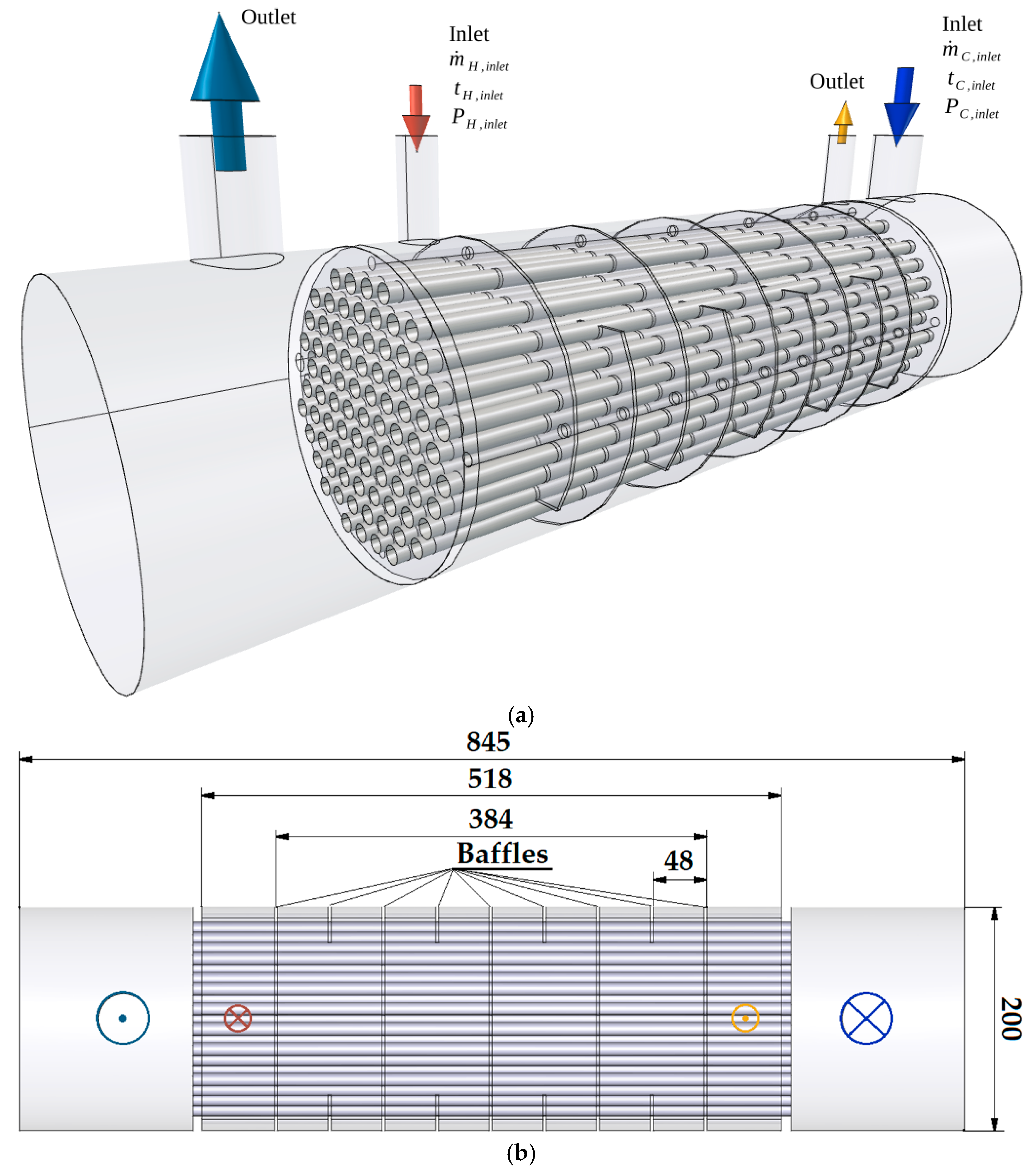
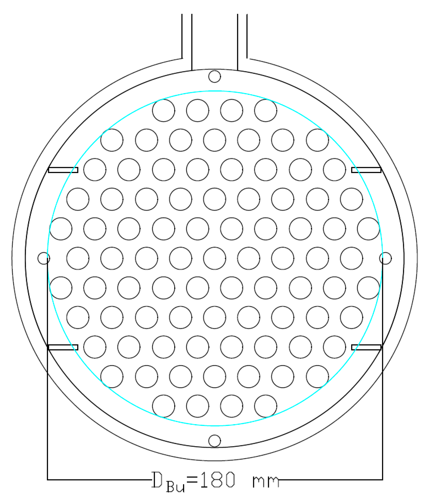
The geometry and dimensions of the analyzed STHEx were adopted from [35]. Figure 1 illustrates the flow arrangement and the principal dimensions of the tested STHEx, whereas Table 1 summarizes the dimensions and the operating conditions.
Table 2 illustrates the gap combinations used in the analysis.

3. Materials and Methods

3.1. Hand Calculation Methods

This study employed two widely accepted and commonly used manual calculation methods: the Bell-D and VDI approaches. Both methods allow for input of thermal-flow parameters, such as mass flow rate and temperature, as well as very detailed data concerning the geometry of the STHEx.

3.1.1. The Bell-Delaware Method

Essentially, the Bell-D method is based on determining the HTC for an ideal tube bundle and applying numerous correction factors that account for, among other things, the effects of clearances between the baffle and the shell, as well as between the baffle and the tube bundle. As the procedures used to determine the correction factors are highly complex, their detailed presentation is beyond the scope of this article. The computational milestones of the Bell-D method are presented in [13,36], while the calculations in this study were based on [37], which provides a step-by-step algorithm for calculating the HTC.

3.1.2. The VDI Method

In essence, the VDI method involves determining the HTC for a single tube and then using several correction factors that account for the complex geometry of the STHEx. Similarly to the Bell-D method, the procedures used to predict the HTC are highly intricate; therefore, their discussion is beyond the scope of this paper. The key computational steps of the VDI method are presented in [14,36], while calculations in this study were based on [38], which provides a step-by-step algorithm for predicting the HTC.

3.2. Numerical Methods

3.2.1. OpenFOAM Approach

The system of equations governing flow with heat transfer can be expressed as
ρ τ + · ρ u = 0
τ ρ u + · ρ u u = ρ g P + · μ u + ·   μ d e v 2 u T
τ ρ K + h + · ρ u K + h = P τ + ρ g · u + · λ h
In the system in Equations (1)–(3), u is the velocity vector, dev2 T = T − 2/3 δtrT, and δ is the unity tensor. The kinetic energy is of the form K = 1/2 ‖u2.
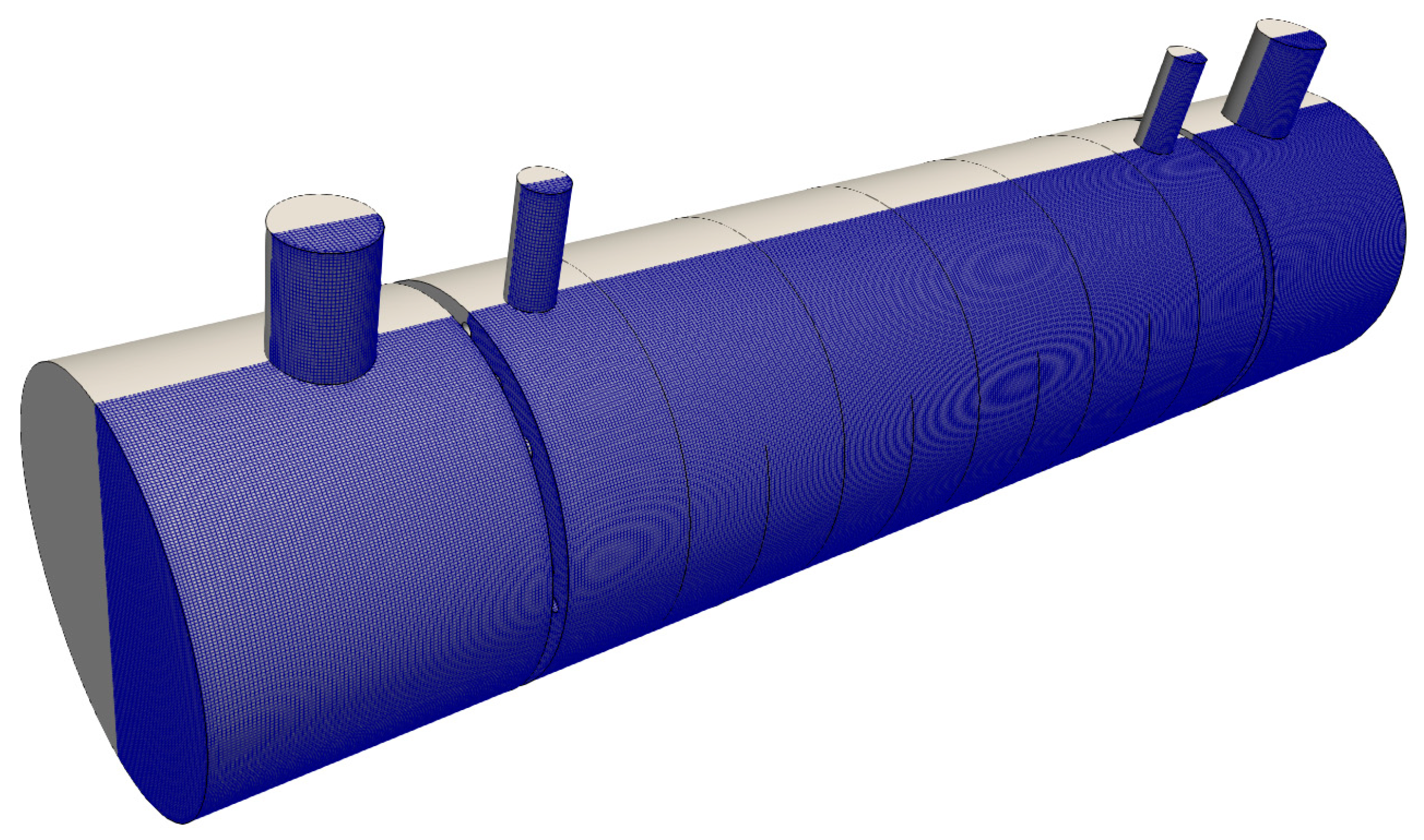
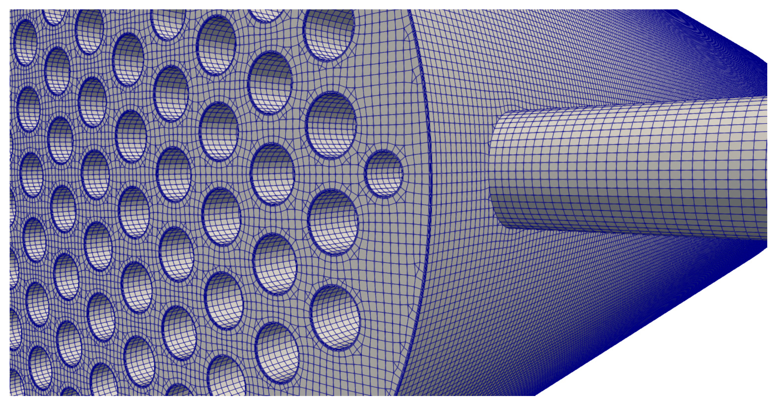
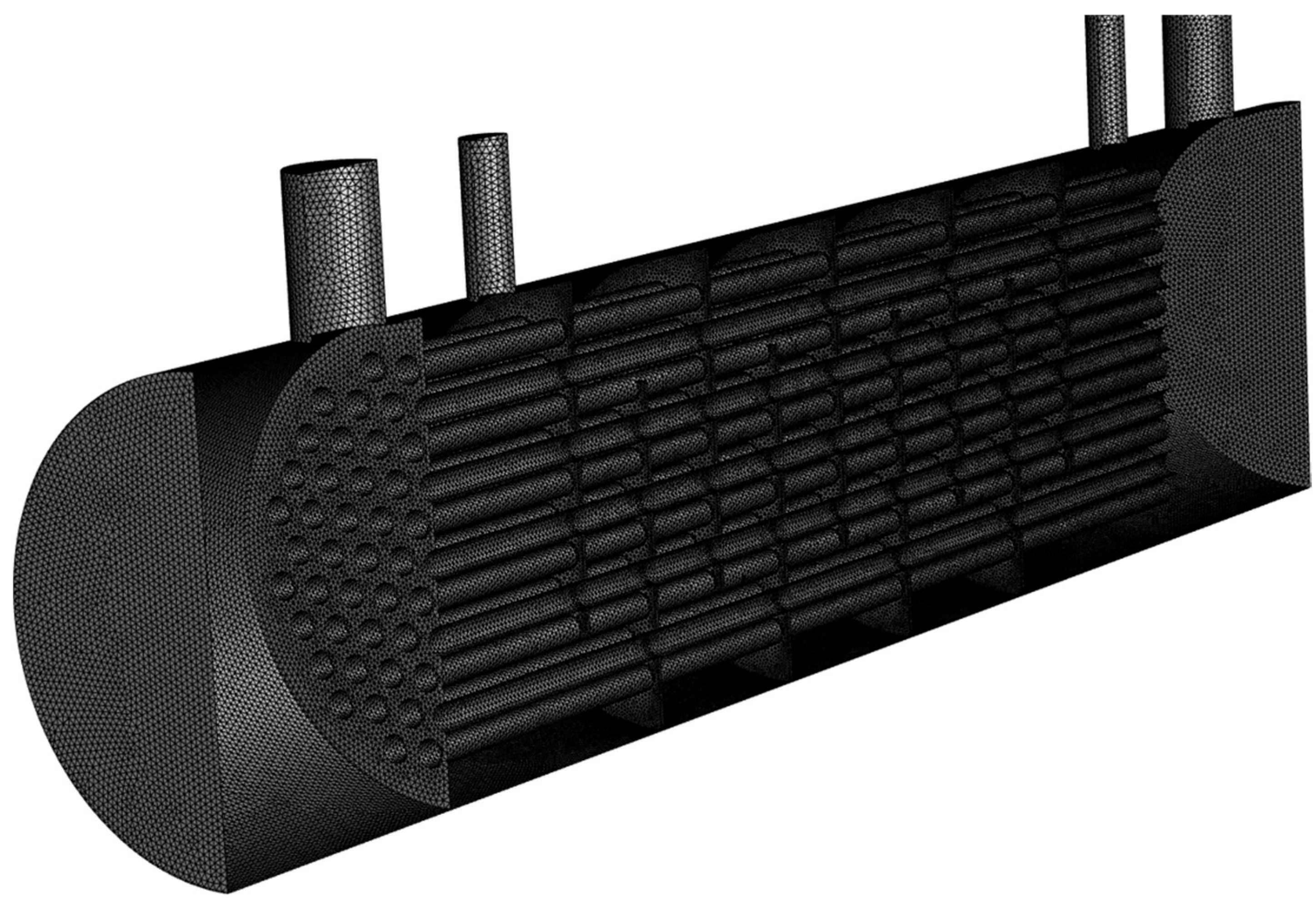
The boundary conditions, such as inlets and outlets to individual domains, are shown in Figure 1. All other surfaces are defined as no-slip walls. The averaged transport Equations (1)–(3) were solved using the Reynolds-Averaged Simulation approach to turbulence, together with the k-ω SST turbulence model [39]. The open-source software OpenFOAM 2312 [40] was used to solve the discretized equations by means of the Finite Volume Method (FVM). The computational Cartesian mesh consisted of 9.92 million nodes—Figure 2. Mesh details near the walls are presented in Figure 3. The SIMPLE algorithm and the GAMG solver were used to solve the system Equations (1)–(3). More details about the OpenFOAM procedure are discussed in [35,36].
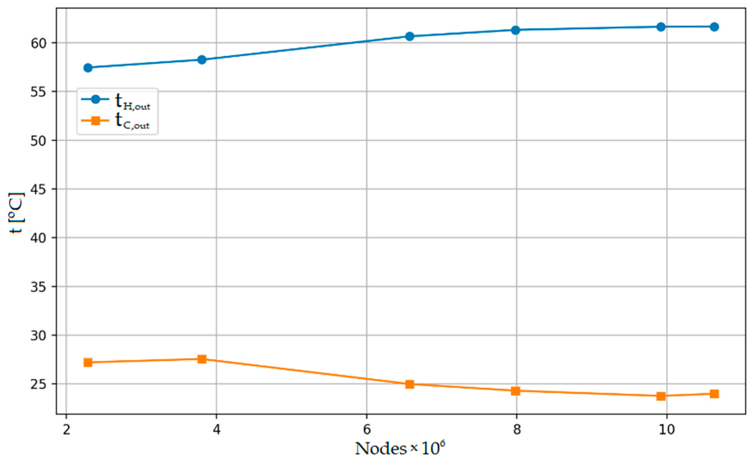
Figure 4 presents the effect of the computational mesh on the outlet temperature of both hot, tH, and cold, tC, fluids. Six cases were examined, spanning from 2.2 million to almost 11 million nodes.
Figure 4 shows that the exit temperature of both hot and cold fluids vary with mesh refinement up to 9.9 million nodes. Further refinement of the mesh does not lead to appreciable changes. A mesh of 9.92 million nodes was therefore selected for subsequent analysis. The mesh sensitivity was investigated for m ˙ H = 2.707 kg/s, tH,in = 77.82 °C, m ˙ C = 3.173 kg/s, and tC,in = 9.81 °C.

3.2.2. Ansys Fluent Approach

Ansys Fluent 21.1 was utilized for conducting the numerical simulations [41]. For the case considered, the system of conservation equations was resolved in the following form
· u = 0
ρ u · u = P + · τ
ρ c p u · T = · λ e f f T
where τ represents the stress tensor including the contributions of molecular and turbulent viscosity of the fluid.
Similarly to the OpenFOAM approach, the boundary conditions, including the inlets and outlets to individual domains, are shown in Figure 1. All other surfaces are defined as no-slip walls. The system of Equations (4)–(6) was solved by means the FVM together with the k-ε turbulence model. The SIMPLE algorithm was applied to solve the pressure–velocity coupling. The computational domain—shown in Figure 5—was generated using the ANSYS Gambit 2.4.6 program (Fluent Inc., Lebanon, NH, USA). Due to geometric symmetry, only half of the domain was simulated. More details about the Ansys Fluent procedure are discussed in [35,36].
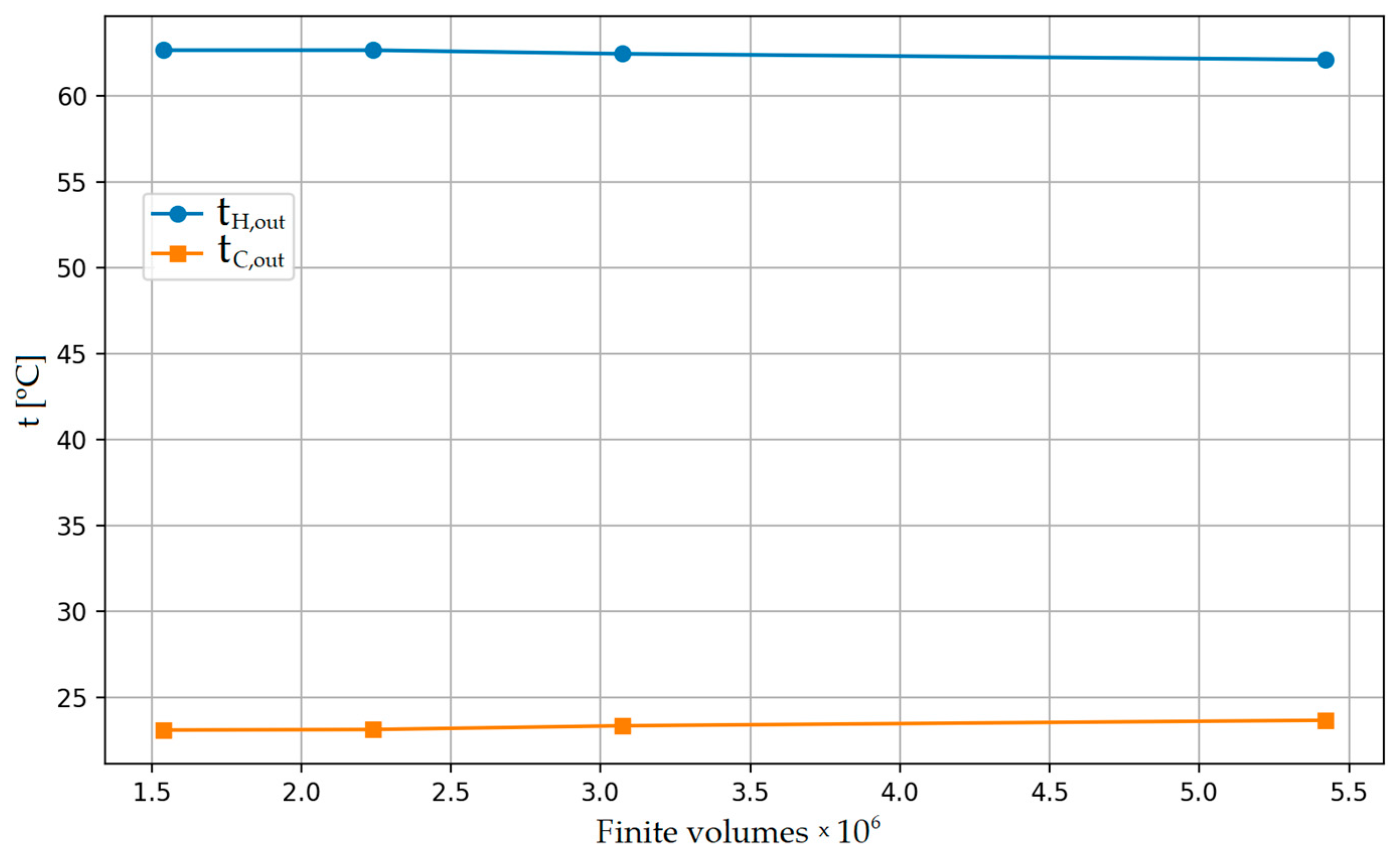
Figure 6 shows the effect of mesh resolution on the exit temperature of both hot, tH,out and cold, tC,out fluids. Four cases were considered, with 1.538 million–5.422 million finite volumes.
Figure 6 indicates that increasing the number of finite volumes from 3.071 million to 5.422 million resulted in an insignificant change in the predicted exit temperatures of both fluids. The mesh sensitivity was investigated for m ˙ H = 3.0 kg/s, tH,in = 75.80 °C, m ˙ C = 3.0 kg/s, and tC,in = 10.0 °C. Since the computation time for the mesh with 5.422 million finite volumes did not differ substantially from that for the mesh with 3.071 million finite volumes, the mesh with the larger number of finite volumes was adopted for further calculations.
Because the k-ω SST and k-ε models are widely used in numerical heat transfer simulations, it was decided to use both in this study. In the modeling of the STHEx, the k-ε model proves effective as a tool for rapid, stable calculations of the system’s overall parameters, whereas the k-ω SST model is more suitable in cases where high local accuracy is crucial—particularly in wall-adjacent regions and in intricate flow inside the shell. Furthermore, the ability of the k-ω SST model to accurately capture near-wall behavior and flow separation phenomena, which predominate inside the shell, has been well documented. This is because the model combines the advantages of the k-ω formulation in near-wall regions and those of the k-ε formulation in the bulk flow. However, the k-ε model is a well-established and reliable approach commonly employed in industrial simulations involving fully developed turbulence, and its computational efficiency and extensive validation studies in the field of heat exchangers make it a suitable reference model for comparative purposes.

3.3. Industrial Software

The academic license under which the calculations were performed does not permit disclosure of the specific correlations used in Aspen Exchanger Design and Rating (Aspen EDR) V15.0 [42]. The shell-side thermohydraulic analysis is performed based on the concept of flow paths in the STHEx originally proposed by Tinker [5,6] and subsequently refined by Palen and Taborek [43]. Aspen EDR is intended primarily for heat exchanger design. However, as demonstrated by the calculations carried out in this study, it also proves to be a highly effective tool for thermohydraulic analysis.

3.4. Water Properties

The properties of hot and cold water were determined using correlations developed on the basis of the database reported in [44]:
-
Dynamic viscosity.
μ = 2.2551418931     3.3948447154   ×   10 2 T   +   2.0532435429   ×   10 4 T 2     6.2294811154   ×   10 7 T 3   +   9.4740755112   ×   10 10 T 4     5.7750953816   ×   10 13 T 5
-
Thermal conductivity.
λ = 2.7689426052   ×   10     4.1570211623   ×   10 1 T   +   2.4968651122   ×   10 3 T 2     7.3889761073   ×   10 6 T 3   +   1.0839020278   ×   10 8 T 4     6.3292341999   ×   10 12 T 5
-
Density.
ρ = 5.8593636805   ×   10 3   +   9.8968557714   ×   10 T     5.7474749375   ×   10 1 T 2   +   1.6856053180   ×   10 3 T 3     2.4989340377   ×   10 6 T 4   +   1.4908022754   ×   10 9 T 5
-
Specific heat.
c p = 1.8561445426   ×   10 5     2.7374285462   ×   10 3 T   +   1.6544683581   ×   10 T 2   5.0060497615   ×   10 2 T 3   +   7.5807970466   ×   10 5 T 4     4.5941525532   ×   10 8 T 5
-
Prandtl number.
Pr = 1130.643576     10.068594 T   +   0.030127 T 2   3   ×   10 3 T 3
The applicable range of Equations (7)–(11) is 10 °C to 80 °C. Within the considered temperature range, the coefficient of determination (R2) equals 1.00000 for dynamic viscosity, thermal conductivity, and density, whereas for specific heat is 0.99987.

4. Results

4.1. An Idealized Heat Exchanger

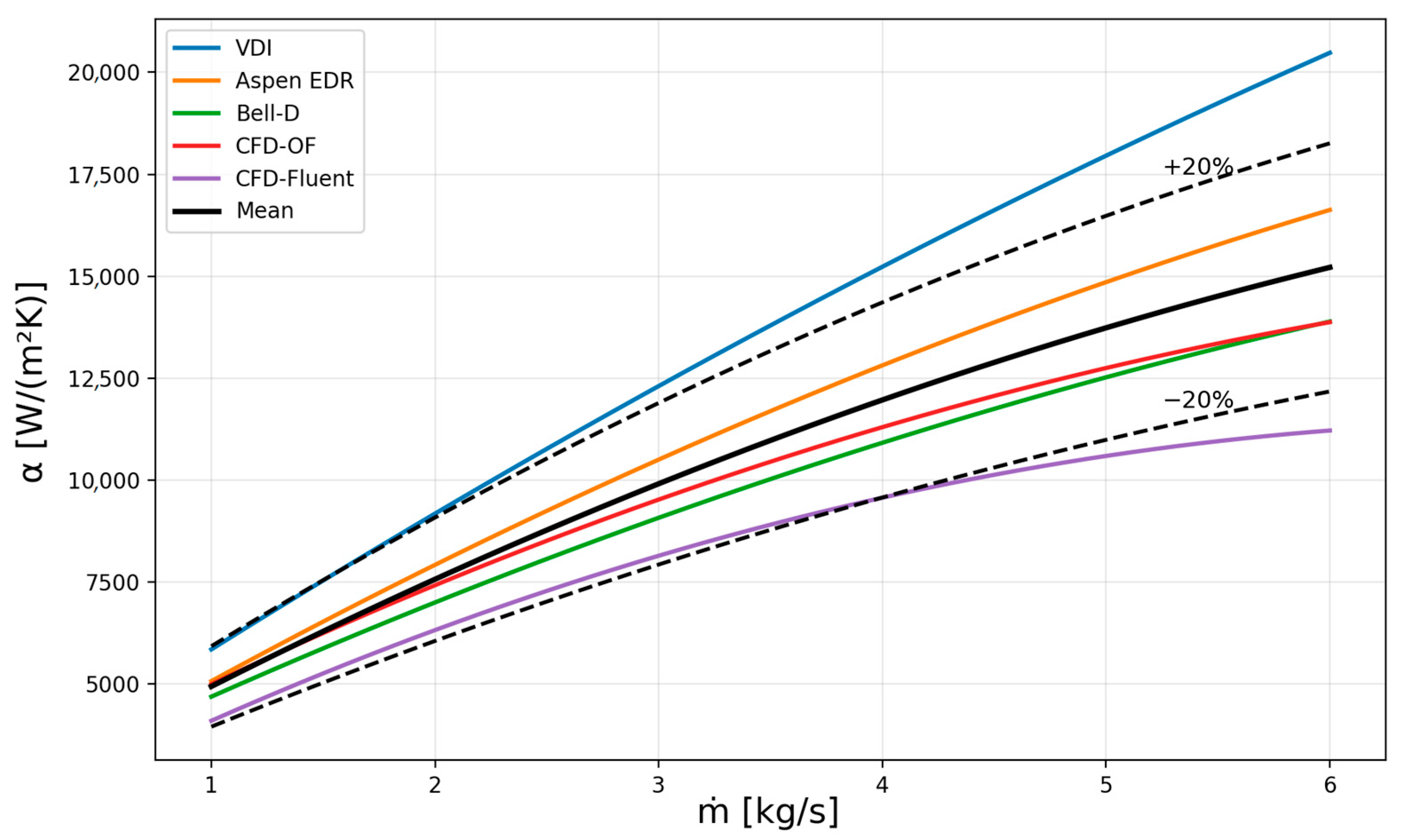
An idealized STHEx is characterized by the absence of leakage between the baffle and the tubes, as well as between the baffle and the shell. However, a bypass stream occurs between the tube bundle and the shell. This fluid stream flows around the outer tubes of the bundle and is therefore not fully utilized for heat transfer. Figure 7 illustrates a comparison of the HTC predicted by all five methods for case A (Table 2).
Figure 7 exhibits that the VDI method predicts the highest HTC, whereas Ansys Fluent yields the lowest value. The discrepancy between the VDI method predictions and the Ansys Fluent results increases as mass flow rate rises, reaching 45% at the highest mass flow rate. The solid black line represents the arithmetic average of the five methods considered, hereafter referred to as the mean. With the exception of the VDI method, the HTCs predicted by the Bell-D method, CFD-OpenFOAM, Ansys Fluent, and Aspen EDR deviate from the mean by no more than ±20%, which indicates close agreement among these methods. The maximum deviation between the values predicted by the VDI method and the mean value was about 34%.
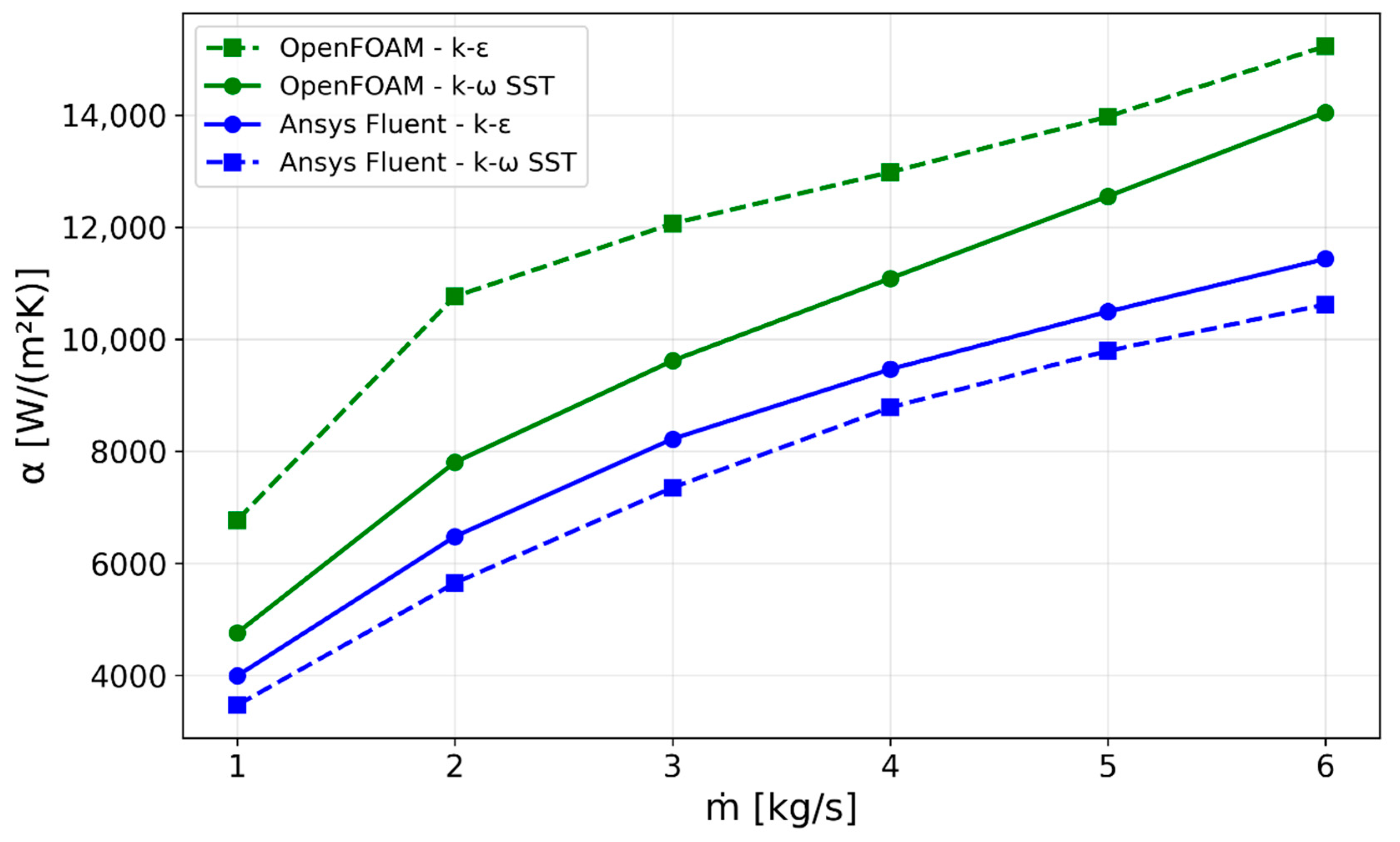
Figure 8 illustrates the HTC predicted by the k-ε and k-ω SST turbulence models for the idealized STHEx corresponding to case A in Table 2.
Figure 8 exhibits that the k-ε formulation implemented in OpenFOAM predicts the highest HTC, while the k-ω SST formulation incorporated in Ansys Fluent yields the lowest. In both CFD approaches, the k-ε turbulence model predicts a higher HTC than the k-ω SST. In the case of OpenFOAM, the discrepancy between the HTC predictions of the k-ε and the k-ω SST models decreases markedly as the mass flow rate increases, amounting to 28% for the lower mass flow rate and 15% for higher mass flow rate. In Ansys Fluent, the discrepancy between the results using the two turbulence models also decreases as the mass flow rate increases, declining from approximately 13% to 7%. The discrepancy between the OpenFOAM predictions and the Ansys Fluent results for the k-ω SST turbulence model decreases slightly as the mass flow rate increases, dropping from approximately 28% to 21%. Similarly, the discrepancy between the OpenFOAM predictions and the Ansys Fluent results for the k-ε model decreases as the mass flow rate increases, falling from approximately 39% to 27%.
Generally, it can be stated that, in Ansys Fluent, the use of either the k-ε or k-ω SST turbulence model does not significantly affect the predicted HTC, whereas for OpenFOAM, the differences in the resulting HTCs are much greater. Importantly, in the case considered, the results obtained with the k-ω SST formulation in OpenFOAM and the k-ε formulation in Ansys Fluent were more consistent than those obtained using the same turbulence model across different computational codes. Therefore, different turbulence models were adopted for the subsequent analysis in the two codes: the k-ω SST in OpenFOAM and the k-ε in Ansys Fluent. It should also be borne in mind that the k-ω SST model provides better handling of near-wall flows, adverse pressure gradients, and flow separation. However, the enhanced predictive capabilities of the k-ω SST model are achieved at the expense of increased computational time. This is because the model is more sensitive to the quality of the computational mesh and requires a correspondingly denser mesh near the wall.
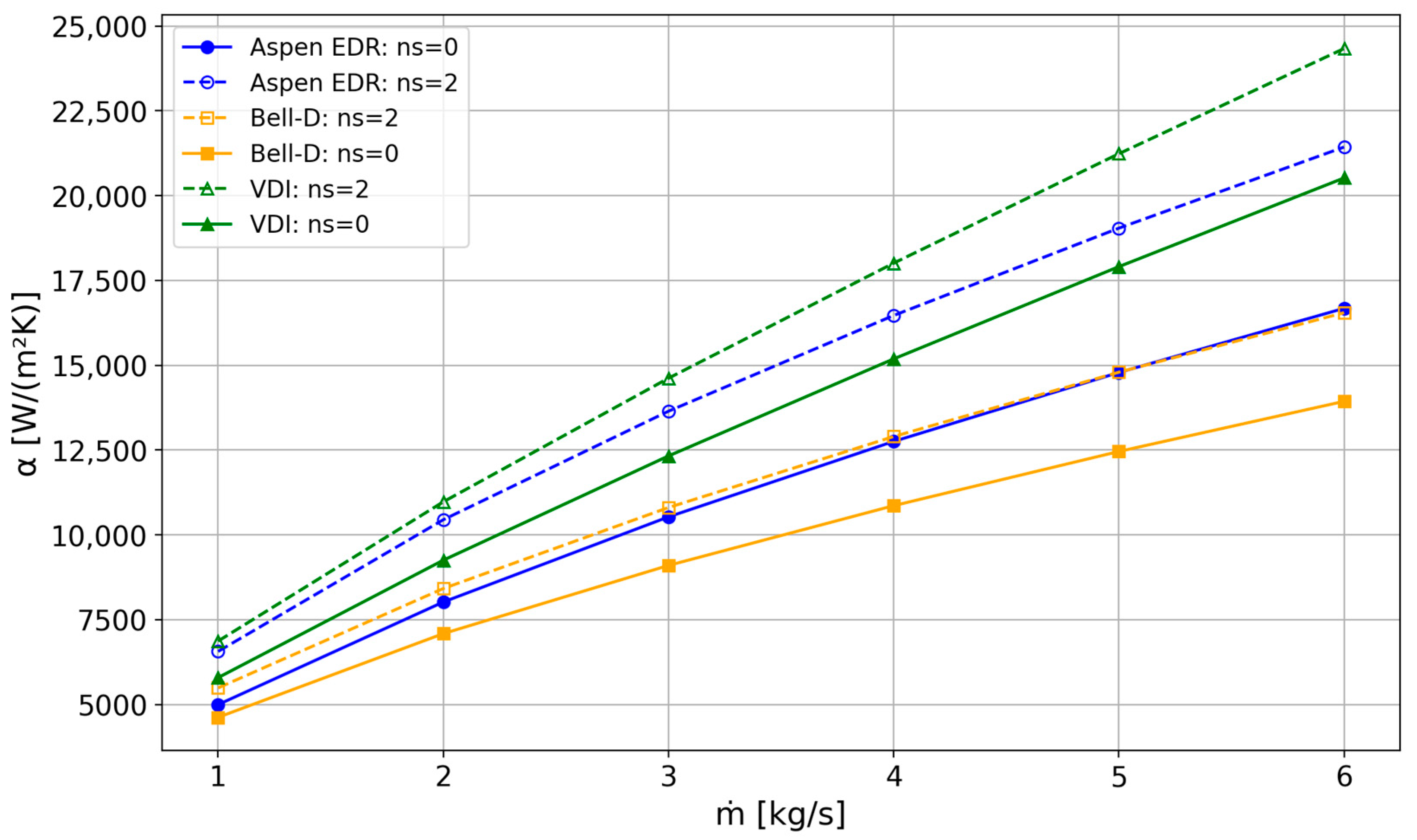
Figure 9 exhibits a cross-sectional view of the idealized STHEx, whereas Figure 10 illustrates the HTC for the cases without and with sealing strips.
Figure 10 exhibits that all three considered methods predict a rise in HTC for the STHEx equipped with sealing strips, as expected, since the sealing strips redirect the bypass stream into cross-flow. While the VDI and Bell-D methods predict virtually the same increase in HTC—18.6% and 18.7%, respectively—regardless of mass flow rate, Aspen EDR yields a rise in HTC of about 30%, which is slightly higher at lower mass flow rates.
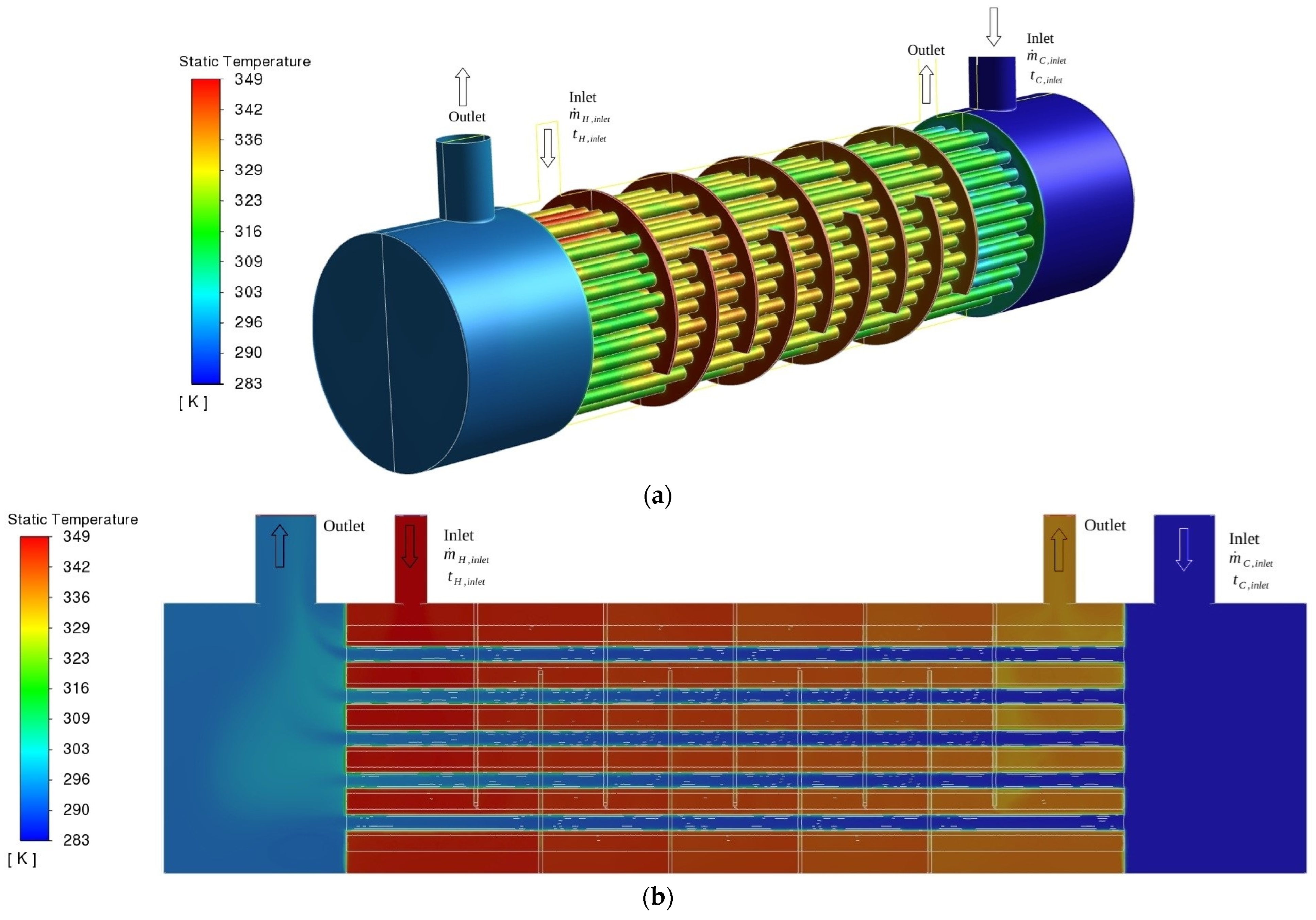
Figure 11 illustrates the temperature distribution obtained from numerical simulations carried out in Ansys Fluent for m ˙ H   = 3 kg/s and m ˙ C   = 3 kg/s, respectively, with inlet temperatures of tH,in = 75.8 °C and tC,in = 10 °C, respectively.
In Figure 11a, the temperature distribution of the baffles is particularly noteworthy. The first three baffles on the hot water inlet side have nearly identical high temperatures, whereas from the fourth baffle onward a clear drop in the baffle temperature can be observed. In Figure 11b, it is characteristic that the hot water temperature drops very sharply already in the first section of the STHEx, which is expected since the hot water comes into contact there with tube surfaces at the lowest temperature, resulting from cold water inlet temperature.
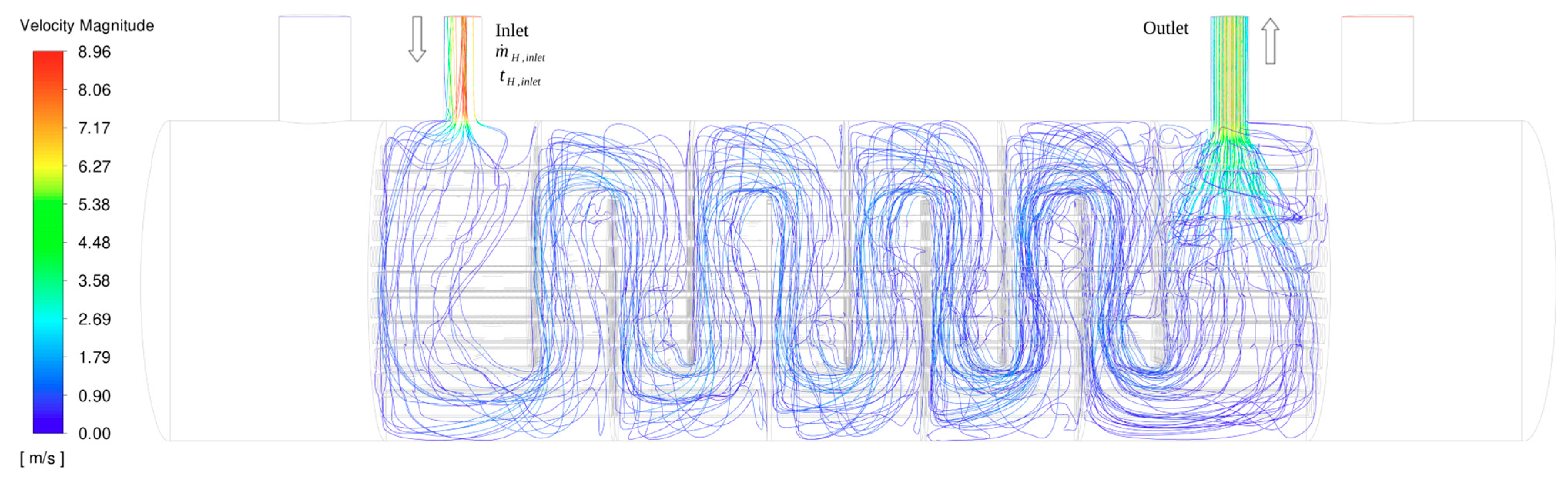
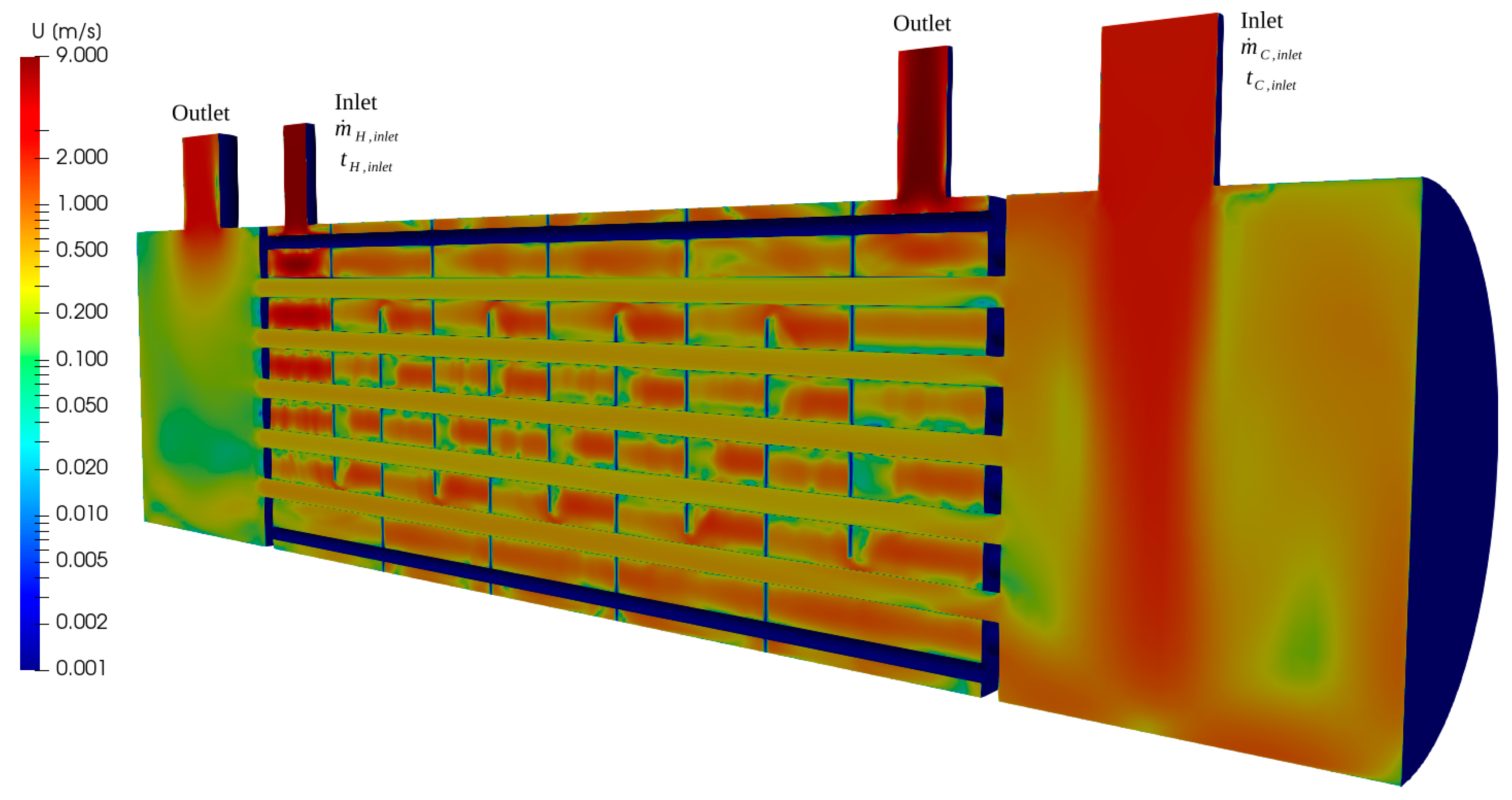
Figure 12 shows the flow map inside the shell of the idealized STHEx for m ˙ H   = 3.0 kg/s.
Figure 12 exhibits that the hot water flow is relatively uniform throughout most of the exchanger, with the exception of the region near the outlet port. The velocity distribution at the outlet port is more uniform than at the inlet port, where a clearly higher velocity is observed along the port axis. Since the case considered involves an idealized STHEx, Figure 12 shows no leakage flows associated with the gaps between the baffle and the tubes or between the baffle and the shell.
Figure 13 shows the velocity distribution in the idealized STHEx.
Figure 13 shows the velocity distributions in the form of vector magnitude in a longitudinal view of the entire unit. The distribution is presented on a logarithmic scale, which permits better visualization of the full range of velocities compared to a linear scale. Figure 13 shows that there are no stagnation zones on either side of the exchanger, which would be represented by dark blue color. In both computational domains, the peak velocities are located in the entrance and exit ports. Localized velocity drops are also visible where the water flows around the baffles. Figure 13 shows that, although the baffles cause the flow to decelerate, these regions are not true stagnation zones, as the velocity remains approximately 0.2 m/s. This local reduction in velocity is accompanied by a slight change in temperature, as shown in Figure 11b. These velocity variations are only visible on a logarithmic scale; otherwise, the distribution would appear uniform.

4.2. Heat Exchanger with Leakage

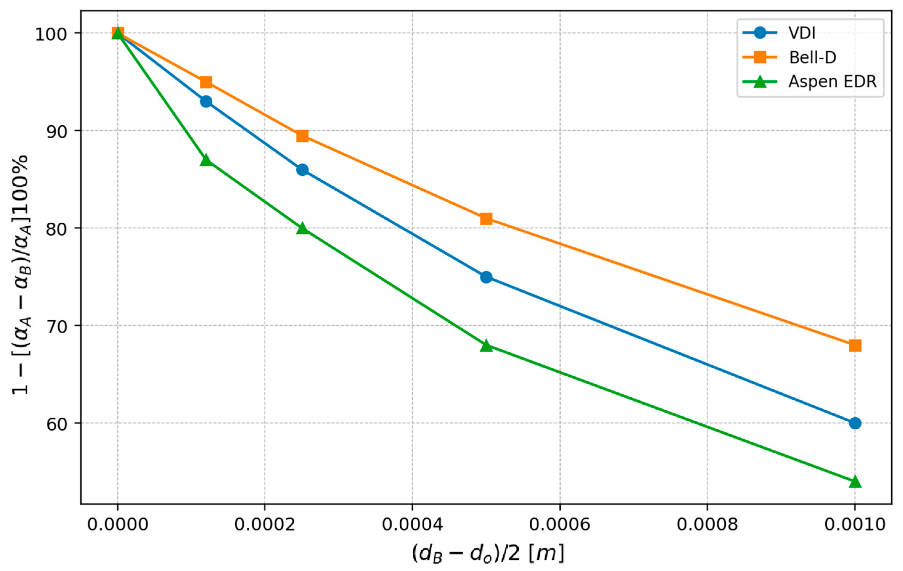
Figure 14 compares the shell-side HTC from the VDI, Bell-D, and Aspen EDR approaches for cases B1 to B4 (Table 2), i.e., for the instances without leakage between the baffle and the shell and with leakage between the baffle and the tubes.
As illustrated in Figure 14, the results show that the HTC decreases as the baffle-to-tube gap increases. This is expected, since baffle-to-tube leakage reduces cross-flow. It should be noted that the decrease in the HTC becomes more pronounced as the clearances increase. At the maximum gap ( δ d = 1 mm), the Bell-D, VDI, and Aspen EDR approaches predict an HTC reduction of about 32%, 40%, and 46%, respectively.
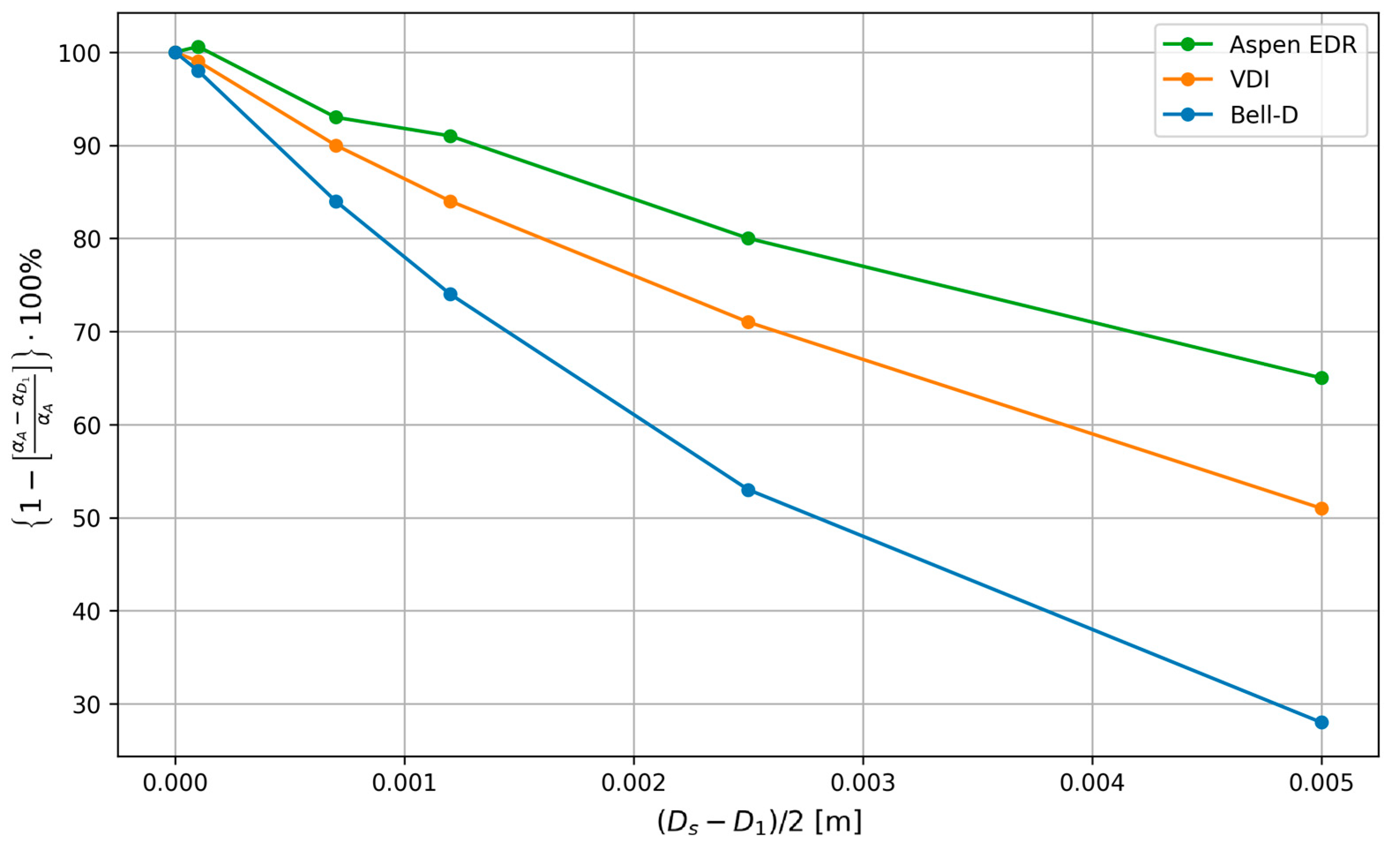
Figure 15 exhibits the variation in the HTC obtained using the VDI, Bell-D, and Aspen EDR approaches with the shell-to-baffle gap for the cases C1–C5 relative to the reference case A (Table 2).
As can be seen from Figure 15, the HTC decreases as the shell-to-baffle gap increases, irrespective of the calculation method applied. This behavior is expected, since a larger shell-to-baffle gap promotes a greater bypass stream, which does not contribute effectively to heat transfer from the tube bundle. The individual methods exhibit different sensitivities to increasing clearances. The most conservative results are obtained with the Bell-D method, which indicates a 72% decrease in HTC for the largest shell-to-baffle gap ( δ D = 5 mm). Aspen EDR is the least sensitive to increasing shell-to-baffle clearances and predicts an HTC decrease of approximately 35% for the largest clearance. The VDI method predicts an HTC reduction of about 50% for the largest clearance.
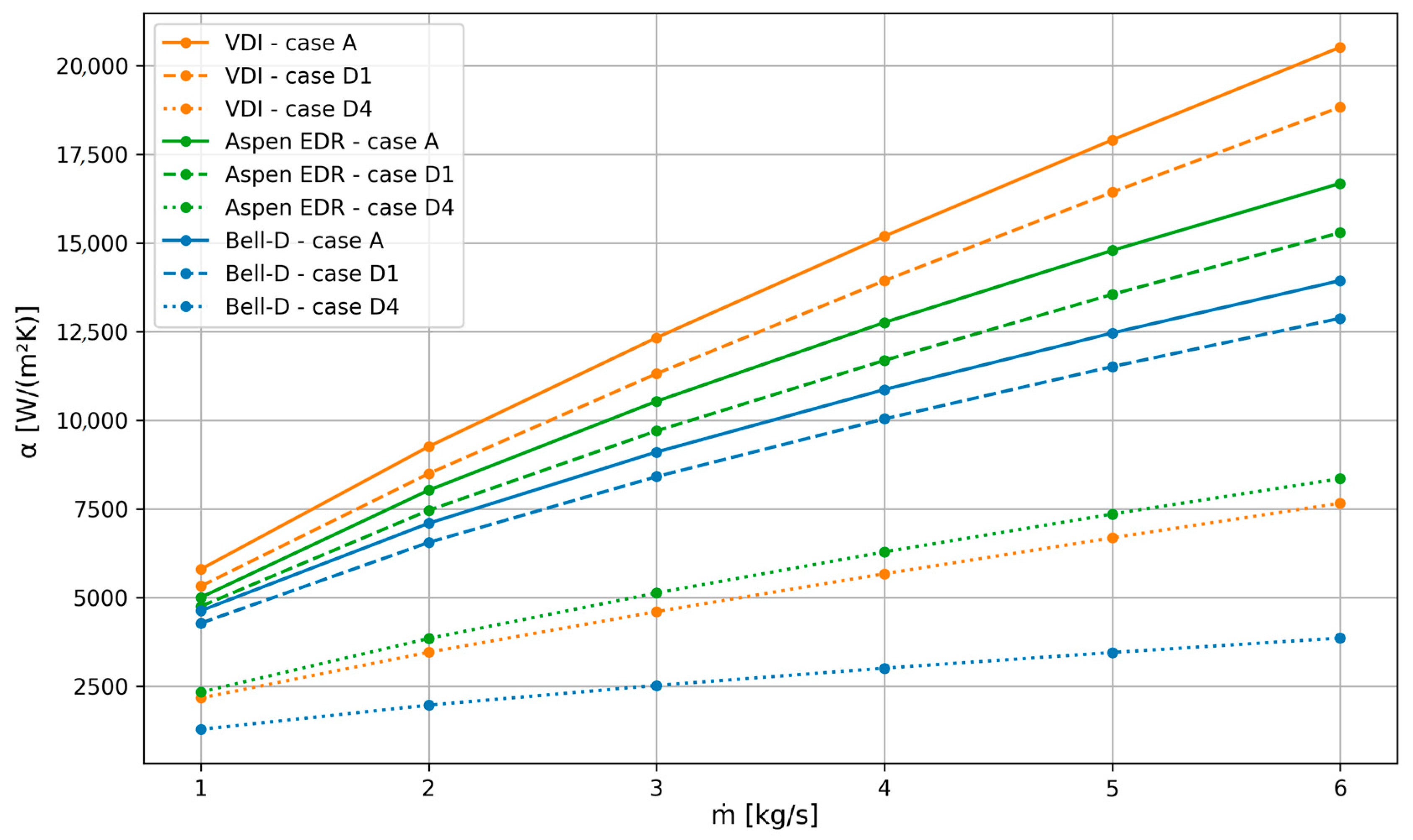
Figure 16 shows the HTC calculated according to the VDI, Bell-D, and Aspen EDR approaches for cases A, D1, and D4 listed in Table 2, which correspond to conditions involving leakage between the baffle and the tubes, as well as between the baffle and the shell.
As can be seen from Figure 16, all three considered methods show a rise in HTC with higher mass flow rate, irrespective of the gap size, from case A with no leakage (solid lines) to case D4 with the maximum values of both types of leakage (dotted lines). Importantly, for case D1 (i.e., for the combination of the smallest gaps, represented by the dashed lines), the considered methods exhibit the same HTC tanking as in case A: the VDI approach yields the highest values, Aspen EDR intermediate, while the Bell-D approach presents the lowest. For case D4, the HTC ranking differs: Aspen EDR predicts the highest HTC values, the VDI method yields intermediate values, while the Bell-D approach gives the lowest.
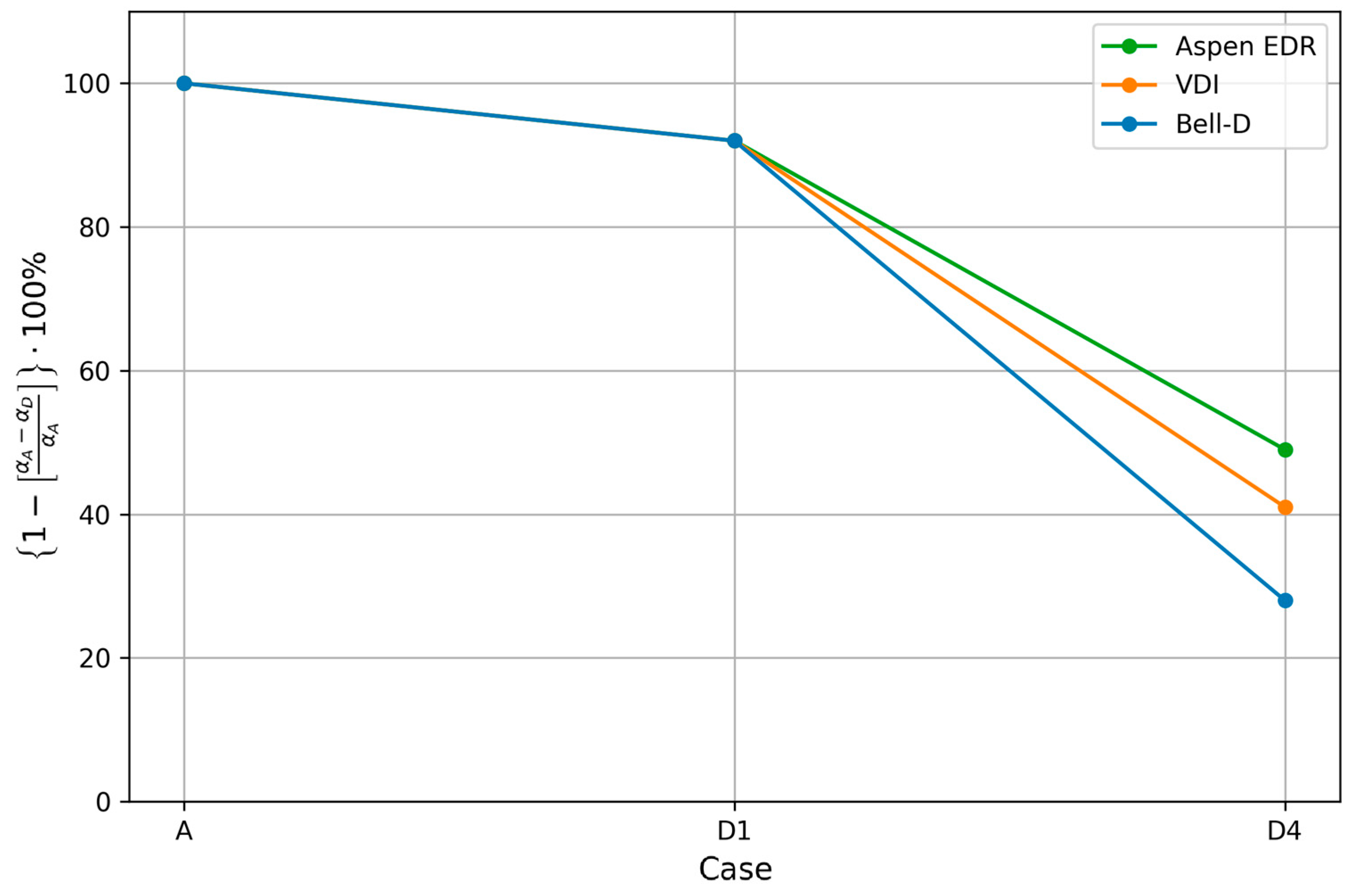
Figure 17 shows the influence of both types of leakage on the HTC, as calculated using the VDI, Bell-D, and Aspen EDR approaches for cases D1 and D4 relative to the reference case A for each method (Table 2).
Figure 17 shows clearly that a reduction in the HTC is predicted by all methods of about 8% for case D1 relative to case A within each respective method. For case D4, however, the situation differs: Aspen EDR, the VDI and Bell-D approaches predict HTC reductions of 55%, 60%, and 65%, respectively, relative to case A.

5. Conclusions

  • Two analytical approaches, namely the VDI method and the extended Bell-D method, two software tools, namely OpenFOAM and Ansys Fluent, as well as Aspen EDR were applied to estimate the shell-side HTC in the STHEx with segmental baffles, considering a wide range of gaps between the baffle and the shell and between the baffle and the tubes as well as varying fluid mass flow rates. This comparative analysis, using analytical methods as the reference benchmark, represents a preliminary stage of a comprehensive study that includes an extensive experimental component for validation.
  • For the idealized STHEx, with the exception of the VDI method, the remaining four methods predict the HTC within ±20% of the mean, defined as the arithmetic average of the results obtained using the five methods considered. The VDI approach overestimates the HTC by approximately 34%.
  • The predictions showed that using two pairs of sealing strips in the idealized STHEx increased the HTC by more than 18% in the VDI and Bell-D approaches, and approximately 30% in Aspen EDR.
  • The calculations showed a strong negative effect of leakage between the baffle and the tubes on the HTC. Specifically, when no shell-to-baffle gap occurs, Aspen EDR predicts a 46% reduction in HTC relative to the idealized STHEx.
  • Shell-to-baffle clearances have a similarly negative impact on the HTC. For the largest clearance-to-shell radius ratio of 5%, and with no leakage between the baffle and the tubes, the Bell-D method predicts an HTC reduction of up to 72% relative to the idealized STHEx.
  • In real STHEx units, both types of leakage occur due to assembly reasons. For the configuration of maximum clearances considered in the calculations, the HTC decreased by at least 50%. The most conservative prediction was obtained with the Bell-Delaware method, which indicated an HTC reduction of about 65% compared with the quasi-ideal STHEx.
  • Both CFD approaches used—OpenFOAM and Ansys Fluent—were found to be highly sensitive to the method used to average the fluid temperature from the computed temperature field (Figure 11), which is a necessary step in determining the HTC.
Future work will include systematic experimental investigations of STHEx units with different baffle configurations.

Author Contributions

Conceptualization, J.T.C.; methodology, J.T.C.; software, J.B., P.D., K.S. and K.T.; validation, J.T.C., J.B., P.D., K.S. and K.T.; formal analysis, J.T.C.; investigation, J.T.C., J.B., P.D., K.S. and K.T.; data curation, J.T.C., J.B., P.D., K.S. and K.T.; writing—original draft preparation, J.T.C.; writing—review and editing, J.T.C., P.D., J.B. and K.T. All authors have read and agreed to the published version of the manuscript.

Funding

This research received no external funding.

Data Availability Statement

The original contributions presented in this study are included in the article. Further inquiries can be directed to the corresponding author.

Conflicts of Interest

The authors declare no conflicts of interest.

Nomenclature

doTube diameter[m]
dBBaffle tube hole diameter[m]
D1Baffle diameter[m]
DBuTube bundle diameter[m]
DsShell diameter[m]
gAcceleration due to gravity [m/s2]
hSpecific enthalpy[J/kg]
m ˙ Mass flow rate[kg/s]
PPressure[Pa]
TTemperature[K]
uVelocity[m/s]
Greek letters
αHeat transfer coefficient[W/(m2K)]
δClearance[m]
λThermal conductivity[W/(mK)]
ρDensity[kg/m3]
μDynamic viscosity[Pas]
Subscripts
ACase A
CCold
effEffective
HHot
inInlet
outOutlet
sShell

Abbreviations

Bell-DBell-Delaware
CFDComputational Fluid Dynamics
FVMFinite Volume Method
HTCHeat Transfer Coefficient
IDInside Diameter
ODOutside Diameter
OFOpenFOAM
STHExShell-and-Tube Heat Exchanger
VDIVerein Deutscher Ingenieure

References

  1. Gupta, J.P. Heat Exchanger and Pressure Vessel Technology; Hemisphere Publishing Corporation: Washington, DC, USA, 1986. [Google Scholar]
  2. Shah, R.K.; Sekulić, D.P. Fundamentals of Heat Exchanger Design; Wiley & Sons, Inc.: Hoboken, NJ, USA, 2003. [Google Scholar]
  3. Thulukkanam, K. Heat Exchanger Design Handbook, 2nd ed.; CRC Press: Boca Raton, FL, USA, 2013. [Google Scholar]
  4. Kakaç, S.; Liu, H.; Pramuanjaroenkij, A. Heat Exchangers: Selection, Rating, and Thermal Design, 4th ed.; CRC Press: Boca Raton, FL, USA; London, UK; New York, NY, USA, 2020. [Google Scholar]
  5. Taborek, J. Survey of Shell-Side Flow Correlations. In Heat Exchanger Design Handbook; Begell House, Inc.: Danbury, CT, USA, 2025. [Google Scholar]
  6. Tinker, T. Shell Side Characteristics of Shell and Tube Heat Exchanger, Parts I–III, General Discussion of Heat Transfer; Institution of Mechanical Engineers: London, UK; ASME: New York, NY, USA, 1951; pp. 84–110. [Google Scholar]
  7. Tinker, T. Shell-Side Characteristics of Shell and Tube Heat Exchanger. J. Heat Transf. 1958, 80, 36–52. [Google Scholar]
  8. Mukherjee, R. Effectively design shell-and-tube heat exchangers. Chem. Eng. Prog. 1998, 94, 21–37. [Google Scholar]
  9. Marzouk, S.A.; Abou Al-Sood, M.M.; El-Said, E.M.S.; Younes, M.M.; El-Fakharany, M.K. A comprehensive review of methods of heat transfer enhancement in shell and tube heat exchangers. J. Therm. Anal. Calorim. 2023, 148, 7539–7578. [Google Scholar] [CrossRef]
  10. Kern, D.Q. Kern’s Process Heat Transfer, 2nd ed.; Wiley & Sons, Inc.: Hoboken, NJ, USA, 2019. [Google Scholar]
  11. Donohue, D.A. Heat Transfer and Pressure Drop in Heat Exchangers. Ind. Eng. Chem. 1949, 41, 2499–2511. [Google Scholar] [CrossRef]
  12. Žukauskas, A. Heat transfer from tubes in crossflow. Adv. Heat Transf. 1972, 8, 93–160. [Google Scholar]
  13. Serth, R.W.; Lestina, T.G. Process Heat Transfer; Elsevier: Amsterdam, The Netherlands, 2014. [Google Scholar]
  14. Gaddis, E.S.; Gnielinski, V. G8 Shell-Side Heat Transfer in Baffled Shell-and-Tube Heat Exchangers. In VDI Heat Atlas; Springer: Berlin/Heidelberg, Germany, 2010; pp. 731–741. [Google Scholar]
  15. Roetzel, W.; Lee, D. Experimental investigation of leakage in shell-and-tube heat exchangers with segmental baffles. Int. J. Heat Mass Transf. 1993, 36, 3765–3771. [Google Scholar]
  16. Kücük, H.; Ünverdi, M.; Yılmaz, M.S. Experimental investigation of shell side heat transfer and pressure drop in a mini-channel shell and tube heat exchanger. Int. J. Heat Mass Transf. 2019, 143, 118493. [Google Scholar] [CrossRef]
  17. Abdelkader, B.A.; Zubair, S.M. The Effect of a Number of Baffles on the Performance of Shell-and-Tube Heat Exchangers. Heat Transf. Eng. 2019, 40, 39–52. [Google Scholar] [CrossRef]
  18. Wills, M.J.N.; Johnston, D.; Harwell, A.E.R.E. A new and accurate hand calculation method for shell-side pressure drop and flow distribution. In Proceedings of the 22nd National Heat Transfer Conference, HTD; ASME: New York, NY, USA, 1984; Volume 36. [Google Scholar]
  19. Abbas, A.; Ismail, T.; Ayub, Z.; Ayub, A.; Cheema, T.A.; Li, W.; Ye, J. Shell Side Single-Phase Experimental Heat Transfer Analysis of a Vertically Oriented Single Segmental Baffle Bundle with Dimpled Tubes. J. Therm. Sci. Eng. Appl. 2020, 12, 011017. [Google Scholar] [CrossRef]
  20. Di Bono, G.; Corcione, M.; Quintino, A. Systematic comparative analysis of Kern and Bell-Delaware methods for the design of shell-and-tube heat exchangers. Appl. Therm. Eng. 2025, 278, 127327. [Google Scholar] [CrossRef]
  21. Zhang, J.F.; Li, B.; Huang, W.J.; Lei, Y.G.; He, Y.L.; Tao, W.Q. Experimental performance comparison of shell-side heat transfer for shell-and-tube heat exchangers with middle-overlapped helical baffles and segmental baffles. Chem. Eng. Sci. 2009, 64, 1643–1653. [Google Scholar] [CrossRef]
  22. Alperen, M.A.; Kayabaşi, E.; Hüseyin Kurt, H. Detailed comparison of the methods used in the heat transfer coefficient and pressure loss calculation of shell side of shell and tube heat exchangers with the experimental results. Energy Sources Part A Recovery Util. Environ. Eff. 2023, 45, 5661–5680. [Google Scholar] [CrossRef]
  23. Mohammadi, K.; Heidemann, W.; Müller-Steinhagen, H. Numerical Investigation of the Effect of Baffle Orientation on Heat Transfer and Pressure Drop in a Shell and Tube Heat Exchanger with Leakage Flows. Heat Transf. Eng. 2009, 30, 1123–1135. [Google Scholar] [CrossRef]
  24. Ozden, E.; Tari, I. Shell side CFD analysis of a small shell-and-tube heat exchanger. Energy Convers. Manag. 2010, 51, 1004–1014. [Google Scholar] [CrossRef]
  25. Mellal, M.; Benzeguir, R.; Sahel, D.; Ameur, H. Hydro-thermal shell-side performance evaluation of a shell and tube heat exchanger under different baffle arrangement and orientation. Int. J. Therm. Sci. 2017, 121, 138–149. [Google Scholar] [CrossRef]
  26. Gómez, A.; Montañés, C.; Cámara, M.; Cubero, A.; Fueyo, N.; Muñoz, J.M. An OpenFOAM-based model for heat-exchanger design in the Cloud. Appl. Therm. Eng. 2018, 139, 239–255. [Google Scholar] [CrossRef]
  27. He, S.; Wang, M.; Tian, W.; Qiu, S.; Su, S.G. Development of an OpenFOAM solver for numerical simulations of shell-and-tube heat exchangers based on porous media model. Appl. Therm. Eng. 2022, 210, 118389. [Google Scholar] [CrossRef]
  28. Arumsari, A.G.; Ginting, P.J. Analysis of Heat Transfer Coefficient of Shell and Tube on Heat Exchanger Using Heat Transfer Research Inch (HTRI) Software. Formosa J. Sustain. Res. 2023, 2, 1175–1184. [Google Scholar] [CrossRef]
  29. Gnielinski, V. New Equations for Heat and Mass Transfer in Turbulent Pipe and Channel Flow. Int. Chem. Eng. 1976, 16, 359–368. [Google Scholar]
  30. Wang, Y.; Liu, K.; Chen, W.; Chen, J.; Wang, K.; Zhou, G. Analysis of stream flow and its impact on thermal performance in shell-side of heat exchangers based on flow dead zone. Appl. Therm. Eng. 2024, 249, 123414. [Google Scholar] [CrossRef]
  31. Adebayo, J.K.; Dare, A.A.; Petinrin, M.O. Performance characteristics of shell and tube heat exchanger using sectoral baffle. J. Eng. Appl. Sci. 2025, 72, 13. [Google Scholar] [CrossRef]
  32. Prithiviraj, M.; Andrews, M.J. Comparison of a Three-Dimensional Numerical Model with Existing Methods for Prediction of Flow in Shell-and-Tube Heat Exchangers. Heat Transf. Eng. 1999, 20, 15–19. [Google Scholar]
  33. Hoang, H.M.K.; Cao, H.-L.; Pham, P.M.Q.; Hajjar, A.; Nguyen, V.L. A novel shell-and-tube heat exchanger design with alternative inclined baffles. Case Stud. Therm. Eng. 2025, 65, 105542. [Google Scholar] [CrossRef]
  34. Ullah, Z.; Ahmad, I.; Samad, A.; Saghir, H.; Ahmad, F.; Kano, M.; Caliskan, H.; Caliskan, N.; Hong, H. Artificial intelligence assisted prediction of optimum operating conditions of shell and tube heat exchangers: A grey-box approach. CAAI Trans. Intell. Technol. 2025, 10, 349–358. [Google Scholar] [CrossRef]
  35. Cieśliński, J.T.; Stasiak, K.; Tesch, K.; Barański, J.; Dąbrowski, P. A Comparative Analysis of Calculation Methods for Flow Resistance in Shell-and-Tube Heat Exchanger with Segmental Baffles. Energies 2026, 19, 1852. [Google Scholar] [CrossRef]
  36. Cieśliński, J.T.; Barański, J.; Dąbrowski, P.; Fabrykiewicz, M.; Stasiak, K.; Tesch, K. Heat Transfer and Pressure Drop in a Shell-and-Tube Heat Exchanger with Segmental Baffles. Energies 2026, 19, 1760. [Google Scholar] [CrossRef]
  37. Thome, J. Wolverine Heat Transfer Engineering Data Book III; Wolverine Tube, Inc.: Shawnee, OK, USA, 2010. [Google Scholar]
  38. Gnielinski, V.; Gaddis, E.S. Berechnung des mittleren Wärmeübergangskoeffizienten im Aussenraum von Rohrbündelwärmeaustauschern mit Segment-Umlenkblechen. Verfahr.-Tech. 1978, 12, 211–217. [Google Scholar]
  39. Menter, F. Two-equations eddy-viscosity turbulence models for engineering applications. AIAA-J. 1994, 32, 1598–1605. [Google Scholar] [CrossRef] [PubMed]
  40. OpenFOAM. Available online: https://www.openfoam.com (accessed on 11 June 2024).
  41. ANSYS Fluent, version 21.1. Fluent 21.1 user’s guide. ANSYS Inc.: Canonsburg, PA, USA, 2018.
  42. AspenTech. Aspen Exchanger Design and Rating, V15.0; AspenTech Inc.: Bedford, MA, USA, 2023. [Google Scholar]
  43. Palen, J.W.; Taborek, J. Solution of Shellside Flow Pressure Drop and Heat Transfer by Stream Analysis Method. Chem. Eng. Prog. Symp. Ser. 1969, 65, 53–63. [Google Scholar]
  44. Lemmon, E.W.; Huber, M.L.; McLinden, M.O. NIST Standard Reference Database 23, Reference Fluid Thermodynamic and Transport Properties (REFPROP), Version 9.0; National Institute of Standards and Technology: Gaithersburg, MD, USA, 2010.
Figure 1. The model STHEx: (a) flow arrangement, (b) principal dimensions.
Energies 19 02114 g001
Figure 2. Computation domain for OpenFOAM.
Energies 19 02114 g002
Figure 3. Mesh details near the walls for OpenFOAM.
Energies 19 02114 g003
Figure 4. Mesh sensitivity for OpenFOAM.
Energies 19 02114 g004
Figure 5. Computational domain and unstructured tetrahedral mesh developed in Ansys Gambit pre-processor.
Energies 19 02114 g005
Figure 6. Mesh sensitivity for Ansys Fluent.
Energies 19 02114 g006
Figure 7. Shell-side HTC from considered five methods.
Energies 19 02114 g007
Figure 8. Comparison of the HTC for different turbulence models.
Energies 19 02114 g008
Figure 9. The idealized STHEx with two pairs of sealing strips.
Energies 19 02114 g009
Figure 10. Influence of sealing strips on the HTC.
Energies 19 02114 g010
Figure 11. Temperature distribution: (a) axonometric view; (b) longitudinal cross section.
Energies 19 02114 g011
Figure 12. Streamlines of hot water in the idealized STHEx.
Energies 19 02114 g012
Figure 13. Velocity distribution in the idealized STHEx.
Energies 19 02114 g013
Figure 14. Effect of baffle-to-tube leakage on the HTC.
Energies 19 02114 g014
Figure 15. Influence of shell-to-baffle leakage on the HTC.
Energies 19 02114 g015
Figure 16. Influence of two leakage types on the HTC.
Energies 19 02114 g016
Figure 17. Relative impact of both clearance types on shell-side HTC.
Energies 19 02114 g017
Table 1. Dimensions and flow parameters of the tested STHEx [35].
ItemValue/Type
Shell inner diameter200 mm
Length of shell518 mm
Total tube number85
OD/ID tube diameter12/10 mm
Tube layoutTriangular (30°)
Tube pitch1.5
Total number of baffles9
Baffle cut25%
Central baffle spacing48 mm
Inlet and outlet sections67 mm
Hot water mass flow rate1–6 kg/s
Cold water mass flow rate3 kg/s
Mean hot water temperature69 °C
Table 2. The set of the analyzed clearances [35].
Case δ d = d B d o / 2 d B δ D = D s D 1 / 2 D 1
A0.00.012000.00.2000
B10.000120.012240.00.2000
B20.000250.012500.00.2000
B30.000500.013000.00.2000
B40.001000.014000.00.2000
C10.00.000120.00010.1998
C20.00.000120.00070.1986
C30.00.000120.00120.1976
C40.00.000120.00250.1950
C50.00.000120.00500.1900
D10.000120.012240.00010.1998
D20.000250.012500.00070.1986
D30.000500.01300.00120.1976
D40.001000.0140.00250.1950
Disclaimer/Publisher’s Note: The statements, opinions and data contained in all publications are solely those of the individual author(s) and contributor(s) and not of MDPI and/or the editor(s). MDPI and/or the editor(s) disclaim responsibility for any injury to people or property resulting from any ideas, methods, instructions or products referred to in the content.