An Efficient Data Cleaning Method for Renewable Energy Power Stations Integrating Anomaly Detection and Feature Enhancement

Abstract
1. Introduction
1.1. Motivation
1.2. Literature Survey
1.3. Our Contributions
- (1)
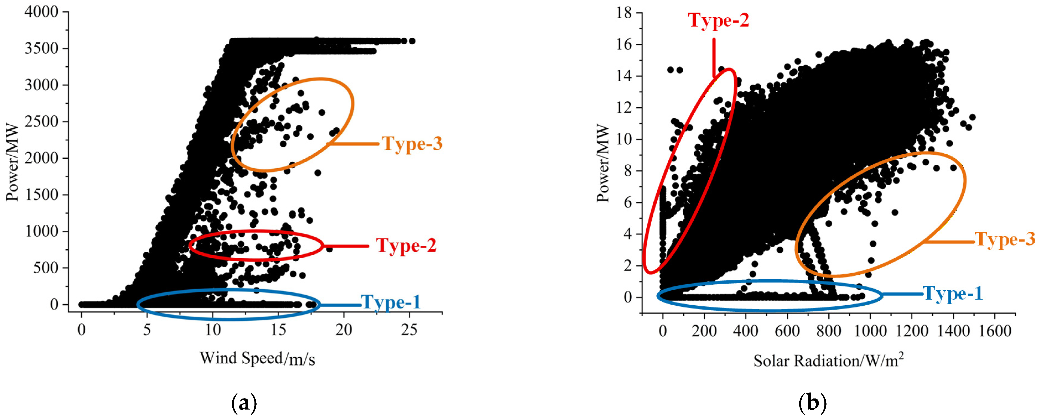
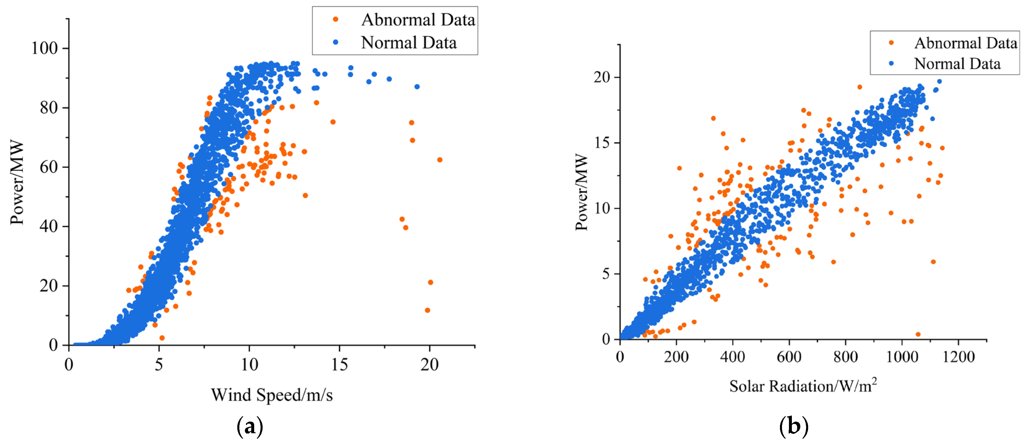
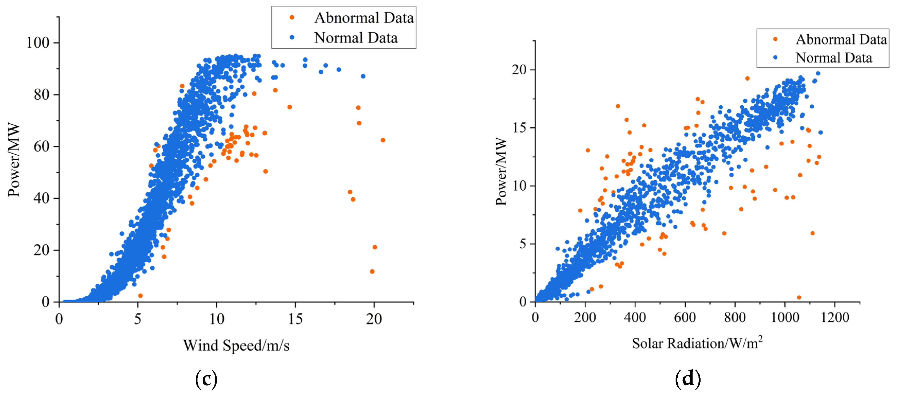
- Adaptive Partitioned Anomaly Detection: Targeting the macroscopic nonlinear density variations in renewable energy data, the Improved DBSCAN algorithm is proposed. By constructing a baseline power curve and utilizing adaptive data partitioning, the density thresholds are dynamically adjusted according to local data density, thereby mitigating the boundary sensitivity defects.
- (2)
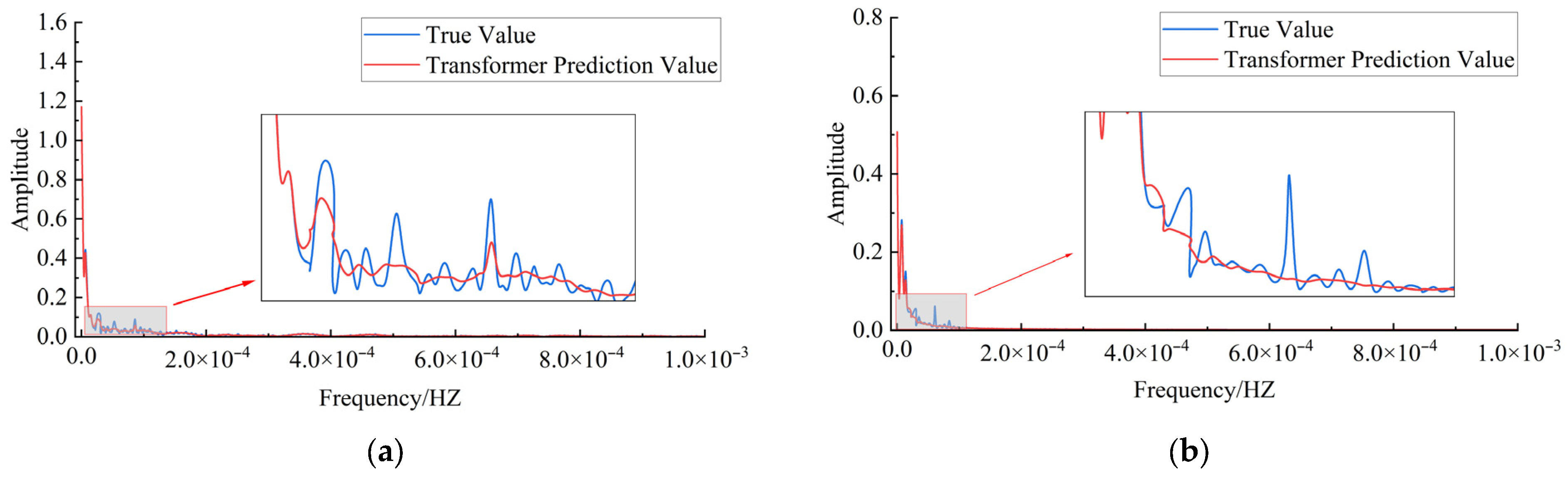
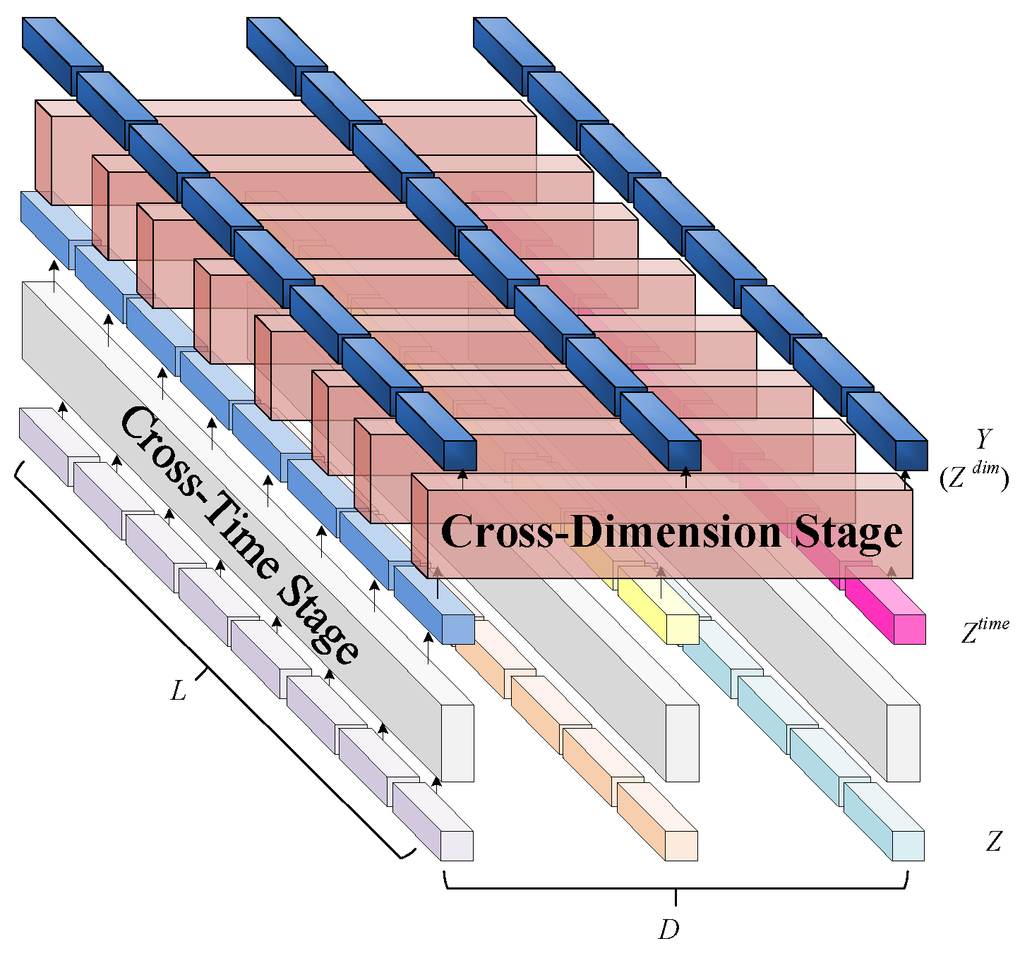
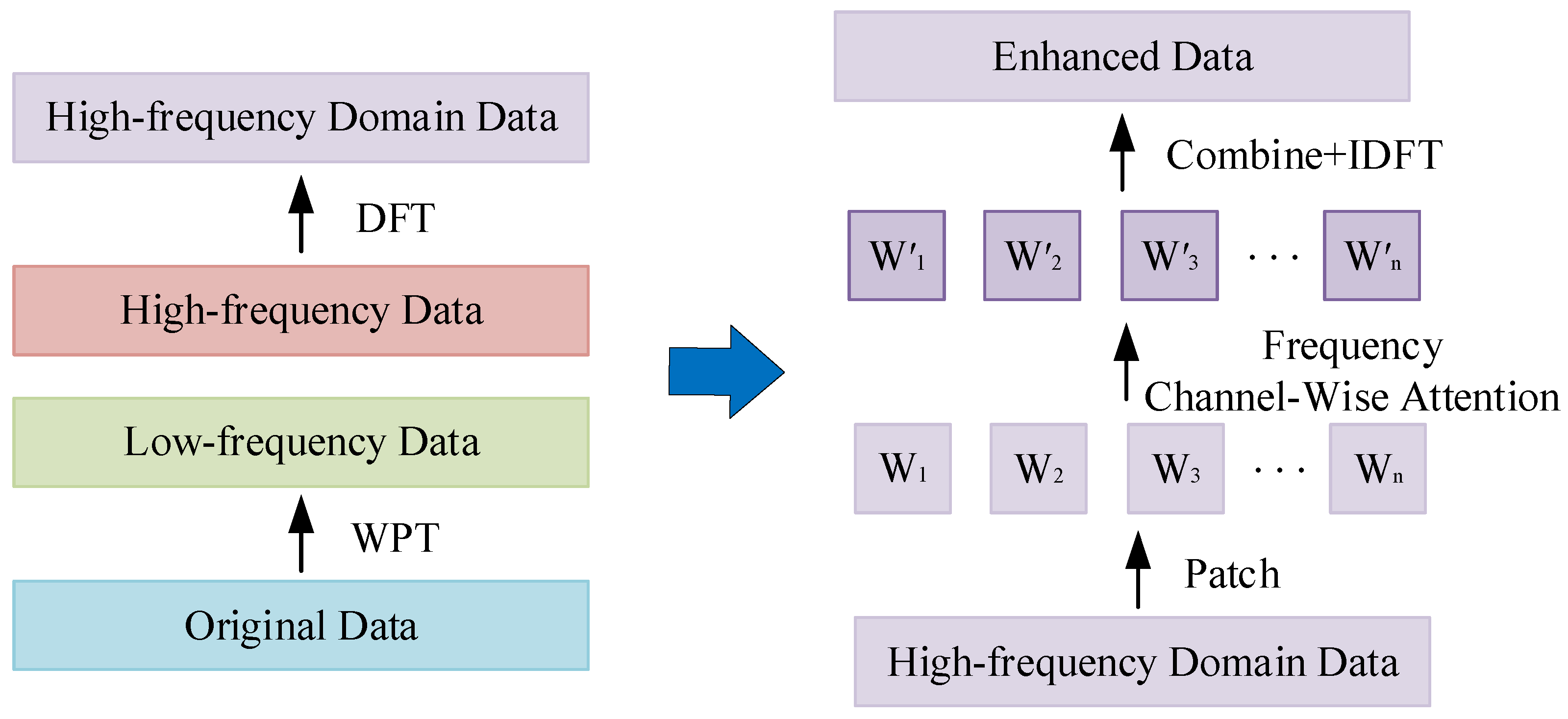
- Decoupled High-/Low-Frequency Feature Enhancement: Addressing the microscopic “frequency bias” in traditional time-series forecasting, a feature enhancement method integrating high–low-frequency decomposition, time–frequency conversion, and an improved attention mechanism is proposed. This forces the network to enhance high-frequency dynamic features that are typically ignored.
- (3)
- Empirical Validation: Based on actual operation data from a renewable energy station in a region of China, the effectiveness of the proposed sequential methodology is verified, demonstrating a significant reduction in prediction errors.
2. Anomaly Data Detection Theory
2.1. Renewable Energy Generator Characteristics Analysis
2.2. Improved DBSCAN Clustering Algorithm
- (1)
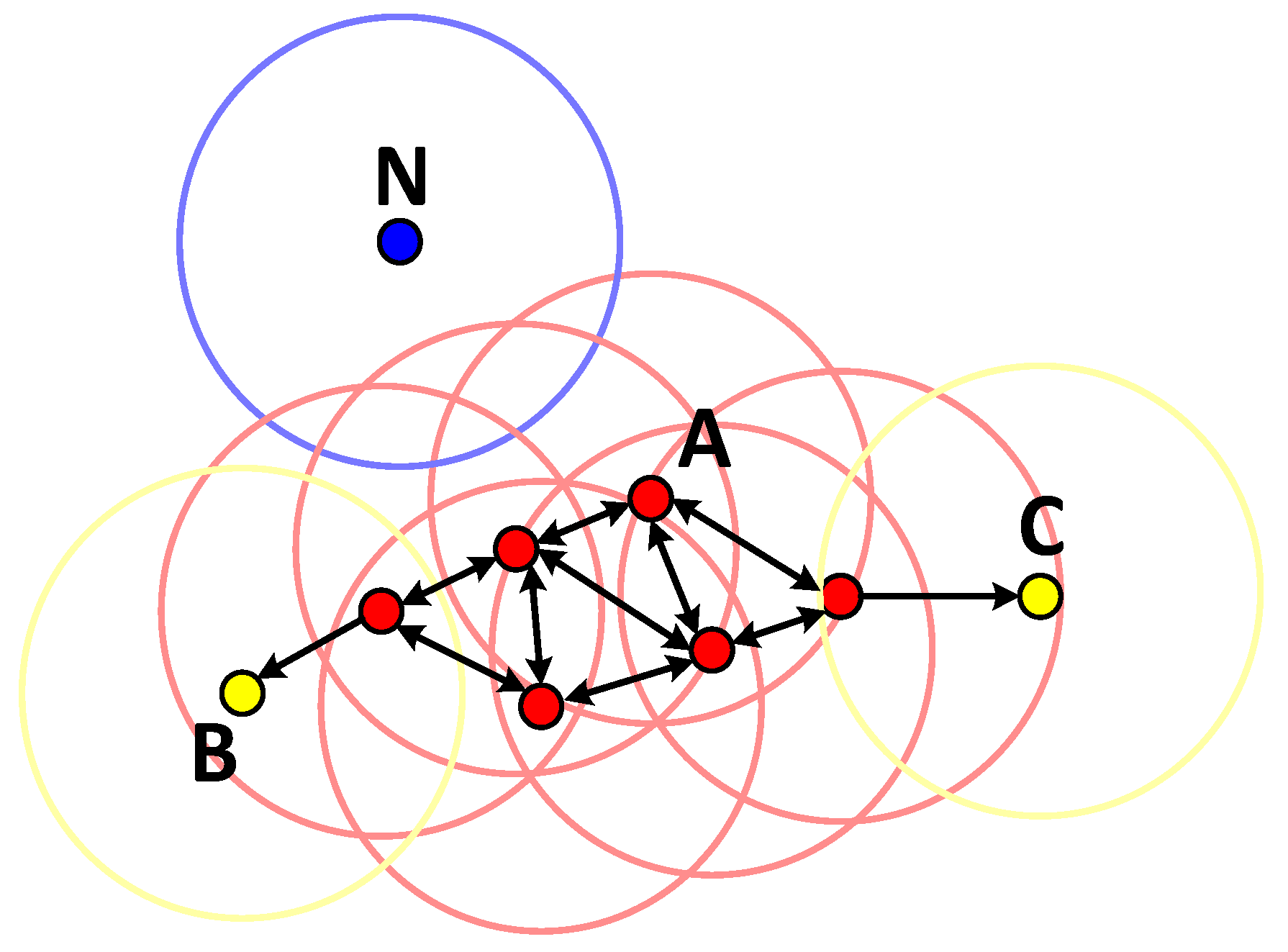
- Core object: An object p is defined as a core object if the number of points contained in its -neighborhood is greater than or equal to the minimum number of points Z:
- (2)
- Directly density-reachable: In the dataset D, if an object p lies within the -neighborhood of an object q, and q satisfies Equation (3) (i.e., q is a core object), then the object q is said to be directly density-reachable from the object p.
- (3)
- Density-reachable: For a given radius and minimum number of points Z, if there exists a chain of objects such that and , and for any adjacent pair pi and pi+1 in the chain, pi+1 is directly density-reachable from pi with respect to and Z, then the object q is said to be density-reachable from the object p with respect to and Z.
- (4)
- Density-connected: If there exists an object such that both object p and object q are density-reachable from object , then the objects p and q are said to be density-connected with respect to and Z.
- (5)
- Clusters and noise: An arbitrary object is selected from the dataset D. Starting from this object p, all points satisfying the threshold Z and the property of density-reachability are searched to form a cluster. Any object that is not contained in any cluster is defined as noise.
- (1)
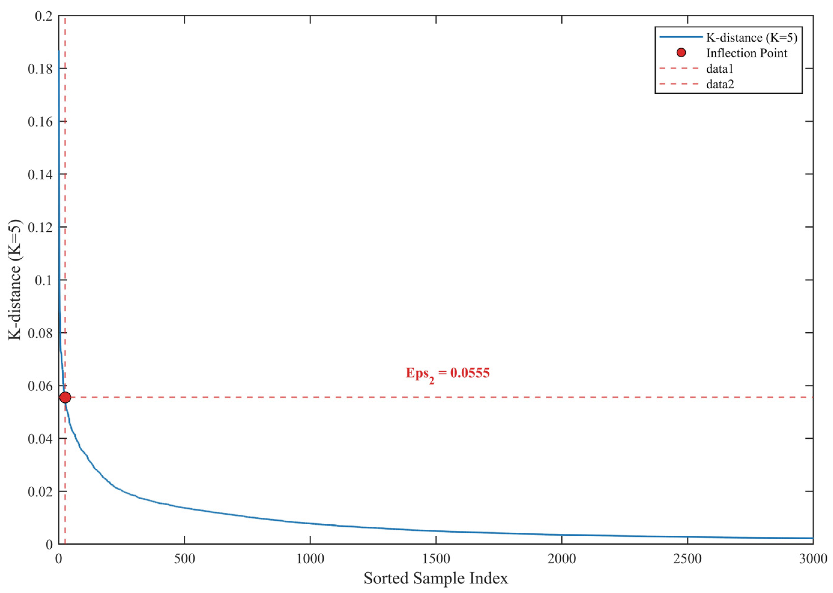
- For each sample point within the dense subset D2, calculate its Euclidean distance to all other sample points in the subset. After sorting the distances in ascending order, the K-th distance is taken as the K-distance of that sample (based on sensitivity analysis validation, this paper adopts K = 5, which yields the optimal overall performance).
- (2)
- Sort the K-distances of all samples in descending order and plot the K-distance curve.
- (3)
- Elbow point determination criterion: The Savitzky–Golay filter (with a window length of 51 and polynomial order of three) is applied to smooth the K-distance curve, eliminating the interference of random noise on the identification of the elbow point. The second derivative of the smoothed curve is calculated, and the point corresponding to the maximum value of the second derivative is taken as the elbow point. This elbow point represents the transition point where the K-distance changes from gradual to steep. The samples before the transition point are densely distributed normal operating data, while the samples after the transition point are sparsely distributed anomalous data. Therefore, the K-distance value corresponding to this elbow point is taken as Eps2. Figure 3 visually illustrates the determination process of Eps2.
- (1)
- Prioritize the denser subset D2 (the subset below the curve), which has a larger sample size and represents the majority of normal operating data, as the baseline. The K-distance method is used to determine Eps2. This is because the dense subset contains most of the normal operating data, and the elbow point feature of its K-distance curve is more pronounced, enabling a more accurate determination of the neighborhood range baseline for normal data and avoiding parameter deviations that could arise if the sparse subset were used as the baseline.
- (2)
- Density-based adaptive adjustment: Based on the ratio of local densities of the two subsets, Eps is inversely adjusted to obtain Eps1 for the sparse subset. For densely distributed regions, the distances between normal samples are smaller, so a smaller Eps is required to distinguish local outliers. For sparsely distributed regions, the distances between normal samples are inherently larger; if the same small Eps as used in dense regions were applied, a large number of normal samples would be misclassified as noise. Therefore, the Eps threshold needs to be adaptively amplified according to the density difference.
- (3)
- Role of overall data density: The overall data density affects the overall distribution of the K-distance curve, thereby influencing the value of the baseline parameter Eps2. Meanwhile, the relative density ratio between the two subsets determines the adjustment magnitude of Eps1 relative to Eps2, addressing the core issue that the traditional DBSCAN with a globally fixed parameter cannot adapt to density variations.
| Algorithm 1. Adaptive DBSCAN Anomaly Detection Based on Baseline Power Curve Partitioning |
| Input: 2D renewable energy dataset D = {(xi, pi)}, rated power Pr Output: Abnormal sample set O, Normal sample set N //Step 1: Build baseline power curve and partition dataset 1: Divide power range into equal intervals with Δp = 0.02 × Pr, 2: For each interval, calculate the average wind speed/irradiance to obtain the baseline curve f(x) via linear interpolation. 3: Split D into sparse subset D1 (pi ≥ f(xi), above curve) and dense subset D2 (pi < f(xi), below curve) //Step 2: Calculate local density of each subset 4: For each subset Di (i = 1, 2): 5: Divide its 2D feature space into 100 × 100 grids, count occupied grid number Mi 6: Compute distribution area Si = Mi × Δx × Δp, local density ρi = |Di|/Si 7: End for //Step 3: Adaptive calculation of DBSCAN core parameters 8: Compute baseline Eps2 for D2 via K-distance method (K = 5): get K-distance curve, smooth with SG filter, take elbow point value as Eps2 9: Calculate adaptive Eps1 = Eps2 × ρ2/ρ1 for sparse subset D1 10: For each subset Di: compute adaptive MinPtsi = ⌈α × ρi × |D|/|Di|⌉ (α = 1.2) 11: End for //Step 4: Block-wise DBSCAN and result merging 12: Run standard DBSCAN on D1 (Eps1, MinPts1) and D2 (Eps2, MinPts2), get abnormal subsets O1, O2 13: Merge abnormal set O = O1 ∪ O2, raw normal set Nraw = D\O 14: Fill gaps in Nraw via linear interpolation to get final normal set N 15: return O, N; |
3. Data Feature Enhancement Theory
3.1. Analysis of the Frequency Learning Bias Issue in Time Series Forecasting
3.2. Wavelet Packet Decomposition-Based Separation of High- and Low-Frequency Features
3.3. Time–Frequency Joint Dual-Channel Attention Feature Enhancement Module
3.3.1. DFT-Based Time–Frequency Domain Conversion Method
3.3.2. Cross-Temporal Attention-Based Feature Enhancement
3.3.3. Frequency-Domain Channel Attention Mechanism
3.3.4. Implementation Process of the Feature Enhancement Method
- (1)
- Separation of high- and low-frequency features: The input time-series data is decomposed using a six-layer wavelet packet decomposition with the db9 wavelet basis. The low-frequency and high-frequency components are identified and separated, achieving effective separation of high- and low-frequency features.
- (2)
- Time–frequency domain conversion: The Discrete Fourier Transform is applied separately to the separated low-frequency and high-frequency components to convert the time-domain signals into frequency-domain sequences, obtaining the frequency-domain characteristics of each component.
- (3)
- Frequency-domain feature enhancement: For the frequency-domain features of the high-frequency components, a frequency-domain channel attention mechanism is employed to adaptively enhance the weights of weak high-frequency features, improving their representational capability. Simultaneously, the frequency-domain features of the low-frequency components are optimized synchronously to preserve core trend information.
- (4)
- Signal reconstruction and output: The enhanced high- and low-frequency time-domain components are reconstructed using a wavelet packet reconstruction algorithm to synthesize the complete feature-enhanced time-series data, which serves as the input for the subsequent power forecasting model.
4. Case Analysis
4.1. Data Source and Evaluation Metrics
4.2. Analysis of Anomaly Detection Effects
4.2.1. Sensitivity Analysis of Core Parameters
4.2.2. Overall Quantitative Performance Evaluation of Anomaly Detection
4.2.3. Comparison of Anomaly Detection Visualization Results
4.3. Analysis of Feature Enhancement Effects
4.3.1. Basis for Selecting Wavelet Packet Decomposition Parameters and Sensitivity Analysis
4.3.2. Sensitivity Analysis of Sliding Window Overlap Ratio
4.3.3. Sensitivity Analysis of High-Frequency Threshold
4.3.4. Analysis of Feature Enhancement Effectiveness
4.4. Performance Analysis and Comparison
5. Conclusions
- (1)
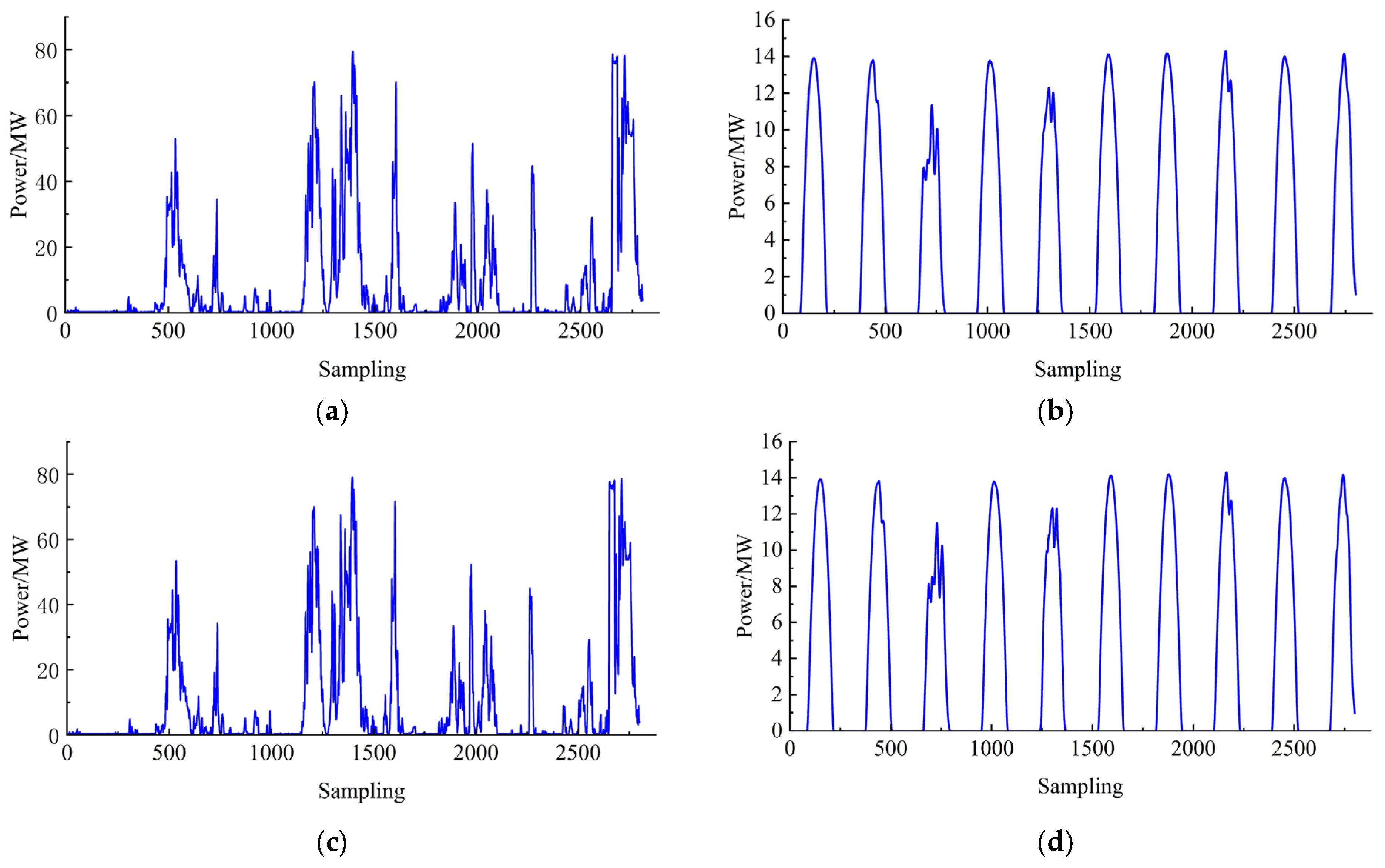
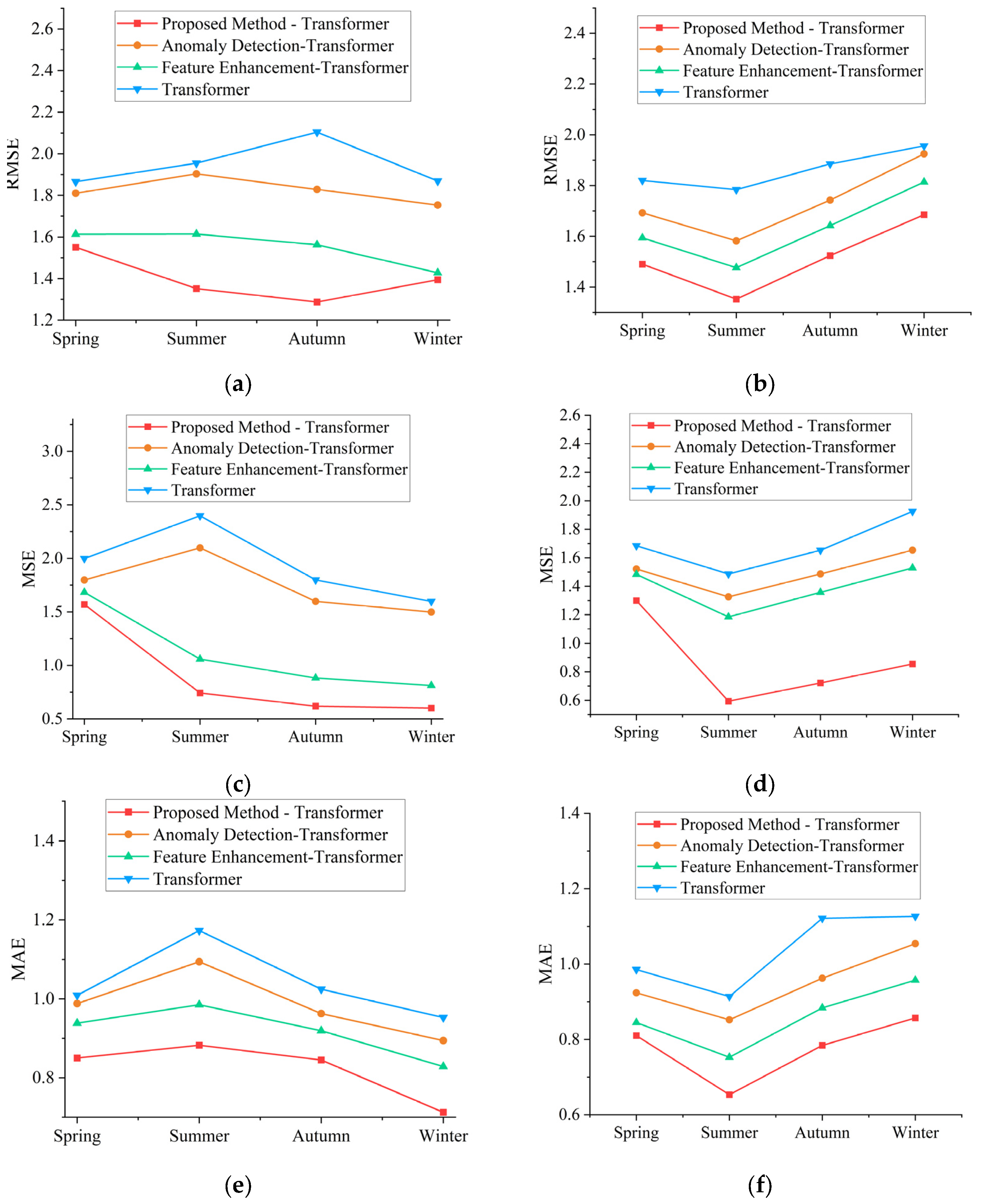
- Considering that DBSCAN has a low ability to identify stacked anomalous data, the original operation data is divided into two parts by constructing a baseline power curve. More accurate anomaly detection is achieved by applying the DBSCAN model to the two subsets, respectively. Anomaly detection not only ensures the quality of power station data but also improves subsequent prediction accuracy. Upon testing, taking the Transformer under wind power data as an example, the proposed method improved its RMSE metric by 3.21%.
- (2)
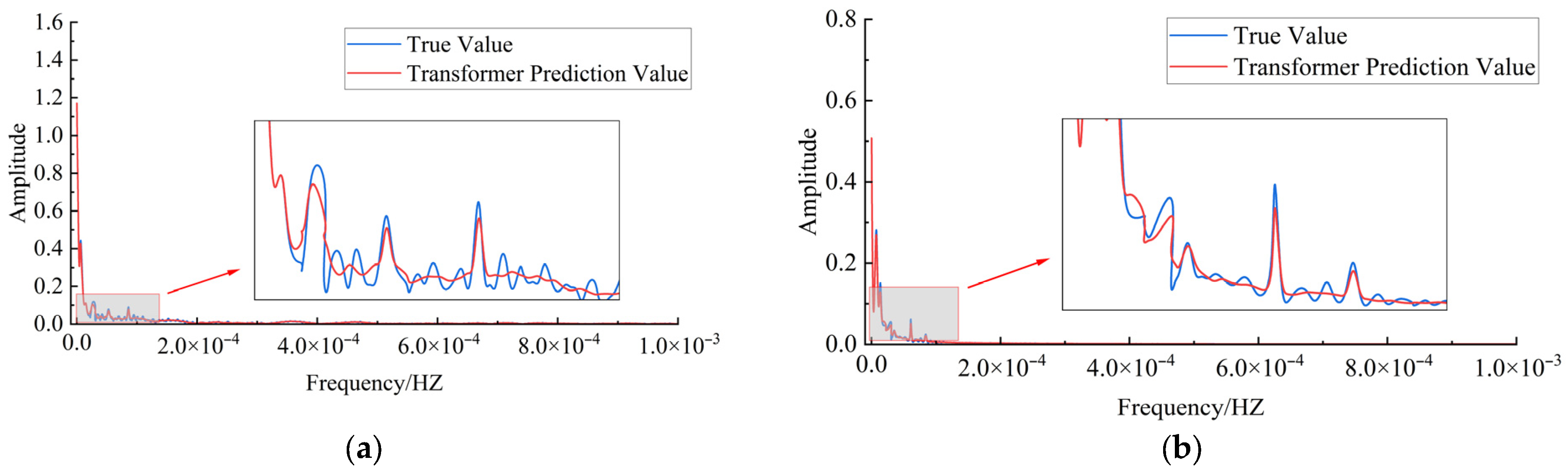
- Aiming at the learning bias problem prevalent in learning networks, this paper used wavelet packet decomposition to achieve the separation of high-frequency data and low-frequency data. Subsequently, the input type was changed through Discrete Fourier Transform, and based on Patch segmentation and dual-channel attention mechanism design, it learned the frequency domain characteristics of the data better, finally realizing the high-frequency feature enhancement of renewable energy data. Through verification, the proposed method successfully made the subsequent prediction network pay attention to the high-frequency information in the data. Taking the Transformer under wind power data as an example, feature enhancement improved its RMSE metric by up to 14.64%.
- (3)
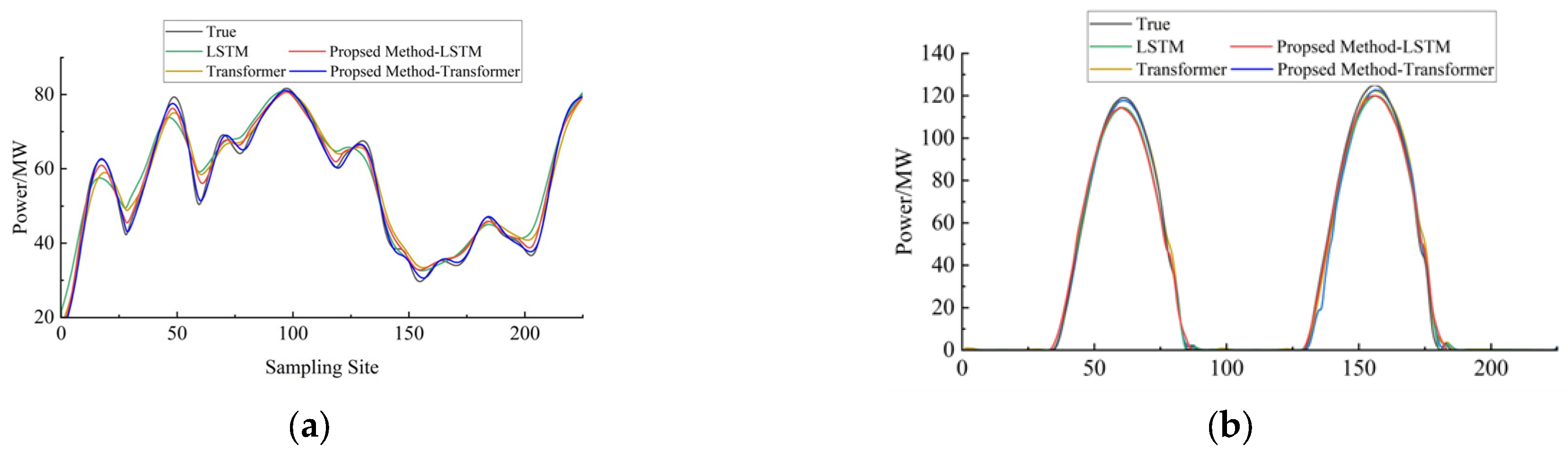
- Different data processing methods are compared with the proposed method. Experimental results show that for renewable energy generation data, the proposed method reduces the Root Mean Square Error (RMSE) of the LSTM and Transformer models by 15.12%, 16.67% and 16.24%, 18.32%, respectively. Compared with other methods, the proposed method is more effective in improving the learning performance of the network.
Author Contributions
Funding
Data Availability Statement
Conflicts of Interest
References
- Yao, Q.; Zhu, H.; Xiang, L.; Su, H.; Hu, A. A novel composed method of cleaning anomaly data for improving state prediction of wind turbine. Renew. Energy 2023, 204, 131–140. [Google Scholar] [CrossRef]
- Mushtaq, K.; Waris, A.; Zou, R.; Shafique, U.; Khan, N.B.; Jameel, M.; Khan, M.I. A comprehensive approach to wind turbine power curve modeling: Addressing outliers and enhancing accuracy. Energy 2024, 304, 131981. [Google Scholar] [CrossRef]
- Ding, J.-W.; Chuang, M.-J.; Tseng, J.-S.; Hsieh, I.-Y.L. Reanalysis and Ground Station data: Advanced data preprocessing in deep learning for wind power prediction. Appl. Energy 2024, 375, 124129. [Google Scholar] [CrossRef]
- Pandit, R.; Wang, J. A comprehensive review on enhancing wind turbine applications with advanced SCADA data analytics and practical insights. IET Renew. Power Gener. 2024, 18, 722–742. [Google Scholar] [CrossRef]
- Zhao, Y.; Ye, L.; Wang, W.; Sun, H.; Ju, Y.; Tang, Y. Data-driven correction approach to refine power curve of wind farm under wind curtailment. IEEE Trans. Sustain. Energy 2017, 9, 95–105. [Google Scholar] [CrossRef]
- Wang, Y.; Infield, D.G.; Stephen, B.; Galloway, S.J. Copula-based model for wind turbine power curve outlier rejection. Wind Energy 2014, 17, 1677–1688. [Google Scholar] [CrossRef]
- Ciulla, G.; D’aMico, A.; Di Dio, V.; Brano, V.L. Modelling and analysis of real-world wind turbine power curves: Assessing deviations from nominal curve by neural networks. Renew. Energy 2019, 140, 477–492. [Google Scholar] [CrossRef]
- Yesilbudak, M. Implementation of novel hybrid approaches for power curve modeling of wind turbines. Energy Convers. Manag. 2018, 171, 156–169. [Google Scholar] [CrossRef]
- Li, W.; Wang, H.; Zhang, Y.; Fang, X.; Tian, X.; Leng, D.; Xie, Y.; Liu, G. Abnormal State Identification Method for Wind Turbines Based on Improved DBSCAN and Random Forests. J. Energy Eng. 2026, 152, 04025110. [Google Scholar] [CrossRef]
- Xiang, L.; Wang, P.; Yang, X.; Hu, A.; Su, H. Fault detection of wind turbine based on SCADA data analysis using CNN and LSTM with attention mechanism. Measurement 2021, 175, 109094. [Google Scholar] [CrossRef]
- Ozcanli, A.K.; Baysal, M. Islanding detection in microgrid using deep learning based on 1D CNN and CNN-LSTM networks. Sustain. Energy Grids Netw. 2022, 32, 100839. [Google Scholar] [CrossRef]
- Li, X.; Zheng, Y. Short-term wind power prediction based on TCN-transformer and STL error correction. In Proceedings of the 2024 IEEE/IAS Industrial and Commercial Power System Asia (I&CPS Asia); IEEE: Piscataway, NJ, USA, 2024; pp. 462–467. [Google Scholar] [CrossRef]
- Alhussein, M.; Aurangzeb, K.; Haider, S.I. Hybrid CNN-LSTM model for short-term individual household load forecasting. IEEE Access 2020, 8, 180544–180557. [Google Scholar] [CrossRef]
- Ren, J.; Yu, Z.; Gao, G.; Yu, G.; Yu, J. A CNN-LSTM-LightGBM based short-term wind power prediction method based on attention mechanism. Energy Rep. 2022, 8, 437–443. [Google Scholar] [CrossRef]
- Al-Ali, E.M.; Hajji, Y.; Said, Y.; Hleili, M.; Alanzi, A.M.; Laatar, A.H.; Atri, M. Solar energy production forecasting based on a hybrid CNN-LSTM-transformer model. Mathematics 2023, 11, 676. [Google Scholar] [CrossRef]
- Xiong, J.; Peng, T.; Tao, Z.; Zhang, C.; Song, S.; Nazir, M.S. A dual-scale deep learning model based on ELM-BiLSTM and improved reptile search algorithm for wind power prediction. Energy 2023, 266, 126419. [Google Scholar] [CrossRef]
- Geng, D.; Wang, B.; Gao, Q. A hybrid photovoltaic/wind power prediction model based on Time2Vec, WDCNN and BiLSTM. Energy Convers. Manag. 2023, 291, 117342. [Google Scholar] [CrossRef]
- Ding, Y.; Chen, Z.; Zhang, H.; Wang, X.; Guo, Y. A short-term wind power prediction model based on CEEMD and WOA-KELM. Renew. Energy 2022, 189, 188–198. [Google Scholar] [CrossRef]
- Zhu, A.; Zhao, Q.; Wang, X.; Zhou, L. Ultra-short-term wind power combined prediction based on complementary ensemble empirical mode decomposition, whale optimisation algorithm, and elman network. Energies 2022, 15, 3055. [Google Scholar] [CrossRef]
- Lydia, M.; Kumar, S.S.; Selvakumar, A.I.; Kumar, G.E.P. Wind resource estimation using wind speed and power curve models. Renew. Energy 2015, 83, 425–434. [Google Scholar] [CrossRef]
- Morrison, R.; Liu, X.; Lin, Z. Anomaly detection in wind turbine SCADA data for power curve cleaning. Renew. Energy 2022, 184, 473–486. [Google Scholar] [CrossRef]
- Wang, H.; Zhang, N.; Du, E.; Yan, J.; Han, S.; Li, N.; Li, H.; Liu, Y. An adaptive identification method of abnormal data in wind and solar power stations. Renew. Energy 2023, 208, 76–93. [Google Scholar] [CrossRef]
- Sardarabadi, A.; Ardakani, A.H.; Matrone, S.; Ogliari, S. Multi-temporal PV power prediction using long short-term memory and wavelet packet decomposition. Energy AI 2025, 21, 100540. [Google Scholar] [CrossRef]
- Zhao, L.; Wen, G.; Wang, J.; Liu, Z.; Huang, X. Transmission tower bolt-loosening time–frequency analysis and localization method considering time-varying characteristics. Struct. Health Monit. 2025, 24, 566–589. [Google Scholar] [CrossRef]
- Tang, J.; Liu, Z.; Hu, J. Spatial-temporal wind power probabilistic forecasting based on time-aware graph convolutional network. IEEE Trans. Sustain. Energy 2024, 15, 1946–1956. [Google Scholar] [CrossRef]
- Song, C.; Cui, J.; Cui, Y.; Zhang, S.; Wu, C.; Qin, X.; Wu, Q.; Chi, S.; Yang, M.; Liu, J.; et al. Integrated STL-DBSCAN algorithm for online hydrological and water quality monitoring data cleaning. Environ. Model. Softw. 2025, 183, 106262. [Google Scholar] [CrossRef]
- Sun, Y.; Li, L.; Yang, F.; Chen, J.; Wang, C. An Algorithm for Abnormality Detection and Failure Diagnosis of Electric Power System Data Collection Based on Deep Learning. In Proceedings of the 2024 International Conference on Big Data Mining and Information Processing; Association for Computing Machinery: New York, NY, USA, 2024; pp. 163–167. [Google Scholar] [CrossRef]
- Zhou, D.; Liu, Y.; Wang, X.; Wang, F.; Jia, Y. Combined ultra-short-term photovoltaic power prediction based on CEEMDAN decomposition and RIME optimized AM-TCN-BiLSTM. Energy 2025, 318, 134847. [Google Scholar] [CrossRef]
- Wu, H.; Hu, T.; Liu, Y.; Zhou, H.; Wang, J.; Long, M. Timesnet: Temporal 2d-variation modeling for general time series analysis. arXiv 2022, arXiv:2210.02186. [Google Scholar] [CrossRef]



| Learning Network | Indicator |
|---|---|
| Precision | |
| Recall | |
| F1 Score |
| Learning Network | Indicator |
|---|---|
| RMSE | |
| MSE | |
| MAE |
| Scenarios | K Value | Precision | Recall | F1 Score |
|---|---|---|---|---|
| Wind power scenario | 3 | 91.23% | 92.56% | 91.89% |
| 4 | 93.15% | 93.87% | 93.51% | |
| 5 | 95.68% | 93.15% | 94.40% | |
| 6 | 94.22% | 92.01% | 93.10% | |
| 7 | 92.87% | 90.56% | 91.70% | |
| Photovoltaic power scenario | 3 | 92.05% | 93.12% | 92.58% |
| 4 | 94.33% | 94.58% | 94.45% | |
| 5 | 96.27% | 94.01% | 95.12% | |
| 6 | 94.89% | 92.75% | 93.81% | |
| 7 | 93.10% | 91.22% | 92.15% |
| Scenarios | α Value | Precision | Recall | F1 Score |
|---|---|---|---|---|
| Wind power scenario | 0.8 | 90.15% | 95.32% | 92.66% |
| 1.0 | 93.58% | 94.02% | 93.80% | |
| 1.2 | 95.68% | 93.15% | 94.40% | |
| 1.4 | 94.25% | 90.36% | 92.26% | |
| 1.6 | 92.11% | 88.25% | 90.14% | |
| Photovoltaic power scenario | 0.8 | 91.02% | 96.18% | 93.53% |
| 1.0 | 94.26% | 94.85% | 94.55% | |
| 1.2 | 96.27% | 94.01% | 95.12% | |
| 1.4 | 94.15% | 91.32% | 93.66% | |
| 1.6 | 93.58% | 90.02% | 91.80% |
| Scenarios | Method | Precision | Recall | F1 Score |
|---|---|---|---|---|
| Wind power scenario | DBSCAN | 82.35 ± 2.14% | 78.62 ± 2.37% | 80.44 ± 2.25% |
| Proposed | 95.68 ± 1.02% ** | 93.15 ± 1.18% ** | 94.40 ± 1.09% ** | |
| Photovoltaic power scenario | DBSCAN | 84.16 ± 1.98% | 80.23 ± 2.15% | 82.15 ± 2.06% |
| Proposed | 96.27 ± 0.94% ** | 94.01 ± 1.05% ** | 95.12 ± 0.98% ** |
| Scenarios | db4 | db6 | db8 | db9 | db10 |
|---|---|---|---|---|---|
| Wind power scenario | 1.72 | 1.66 | 1.60 | 1.55 | 1.53 |
| Photovoltaic power scenario | 1.61 | 1.56 | 1.51 | 1.49 | 1.53 |
| Scenarios | 3-Level | 4-Level | 5-Level | 6-Level | 7-Level | 8-Level |
|---|---|---|---|---|---|---|
| Wind power scenario | 1.85 | 1.73 | 1.72 | 1.55 | 1.58 | 1.64 |
| Photovoltaic power scenario | 1.73 | 1.71 | 1.53 | 1.49 | 1.57 | 1.52 |
| Scenarios | 0.1 | 0.2 | 0.3 | 0.4 | 0.5 |
|---|---|---|---|---|---|
| Wind power scenario | 1.72 | 1.62 | 1.55 | 1.57 | 163 |
| Photovoltaic power scenario | 1.57 | 1.53 | 1.49 | 1.57 | 1.59 |
| Scenarios | 5 × 10⁻⁵ Hz | 8 × 10⁻⁵ Hz | 1 × 10⁻⁴ Hz | 2 × 10⁻⁴ Hz | 5 × 10⁻⁴ Hz |
|---|---|---|---|---|---|
| Wind power scenario | 1.68 | 1.61 | 1.55 | 1.60 | 1.69 |
| Photovoltaic power scenario | 1.59 | 1.51 | 1.49 | 1.52 | 1.56 |
| Scenarios | Method | Precision | Recall | F1 Score |
|---|---|---|---|---|
| Wind power scenario | Improved DBSCAN | 88.37 ± 1.87% | 81.26 ± 2.05% | 84.67 ± 1.96% |
| Autoencoder–CNN + LSTM | 92.45 ± 1.36% | 90.18 ± 1.42% | 91.30 ± 1.39% | |
| Proposed | 95.68 ± 1.02% ** | 93.15 ± 1.18% ** | 94.40 ± 1.09% ** | |
| Photovoltaic power scenario | Improved DBSCAN | 89.56 ± 1.75% | 82.47 ± 1.93% | 85.87 ± 1.84% |
| Autoencoder–CNN + LSTM | 93.12 ± 1.24% | 91.05 ± 1.31% | 92.07 ± 1.27% | |
| Proposed | 96.27 ± 0.94% ** | 94.01 ± 1.05% ** | 95.12 ± 0.98% ** |
| Model | Hyperparameter Configuration |
|---|---|
| CEEMDAN-TCN | Batch size: 128; adaptive noise coefficient ε = 0.2, ensemble number E = 100, maximum decomposition level L = 8, standard deviation of white noise set to 0.2 times the standard deviation of the original signal; 4-layer causal convolutional layers, kernel size k = 3, dilation factors d = [1, 2, 4, 8], number of hidden channels C = 64, no attention mechanism; and learning rate: 0.05, Adam optimizer. |
| Timesnet | Batch size: 128; d_model = 128, number of layers = 2, number of frequency blocks = 3, 2D convolutional kernel size 3 × 3, FFN dimension = 256; dropout rate: 0.1; and learning rate: 0.05, Adam optimizer. |
| LSTM | Batch size: 128; 3 hidden layers with 20 hidden units per layer; dropout rate 0.1; and learning rate: 0.05, Adam optimizer. |
| Transformer | Batch size: 128; d_model = 128, 8-head multi-head attention; dropout rate 0.1; and learning rate: 0.05, Adam optimizer. |
| Network | Indicators | Method | ||||||
|---|---|---|---|---|---|---|---|---|
| Non | CEEMDAN-TCN | Timesnet | Proposed Method | |||||
| Metric Value | Metric Value | Improvement | Metric Value | Improvement | Metric Value | Improvement | ||
| LSTM | RMSE | 1.65 ± 0.08 | 1.47 ± 0.07 * | 10.91% | 1.44 ± 0.06 * | 12.73% | 1.40 ± 0.05 ** | 15.12% |
| MAE | 1.24 ± 0.06 | 1.12 ± 0.05 * | 9.68% | 1.09 ± 0.05 * | 12.10% | 1.06 ± 0.04 ** | 14.01% | |
| MSE | 2.31 ± 0.12 | 1.96 ± 0.10 * | 15.15% | 1.90 ± 0.09 * | 17.75% | 1.88 ± 0.08 ** | 18.45% | |
| Transformer | RMSE | 1.86 ± 0.09 | 1.68 ± 0.08 * | 9.68% | 1.62 ± 0.07 * | 12.90% | 1.55 ± 0.06 ** | 16.67% |
| MAE | 1.01 ± 0.05 | 0.90 ± 0.04 * | 10.89% | 0.88 ± 0.04 * | 12.87% | 0.87 ± 0.03 ** | 13.86% | |
| MSE | 1.99 ± 0.11 | 1.70 ± 0.09 * | 14.57% | 1.59 ± 0.08 * | 20.10% | 1.58 ± 0.07 ** | 20.69% | |
| Network | Indicators | Method | ||||||
|---|---|---|---|---|---|---|---|---|
| Non | CEEMDAN-TCN | Timesnet | Proposed Method | |||||
| Metric Value | Metric Value | Improvement | Metric Value | Improvement | Metric Value | Improvement | ||
| LSTM | RMSE | 2.13 ± 0.10 | 1.87 ± 0.09 * | 12.21% | 1.83 ± 0.08 * | 14.08% | 1.78 ± 0.07 ** | 16.24% |
| MAE | 1.14 ± 0.07 | 1.02 ± 0.06 * | 10.53% | 0.99 ± 0.05 * | 13.16% | 0.97 ± 0.05 ** | 14.88% | |
| MSE | 1.93 ± 0.13 | 1.62 ± 0.11 * | 16.06% | 1.58 ± 0.10 * | 18.13% | 1.56 ± 0.09 ** | 19.10% | |
| Transformer | RMSE | 1.82 ± 0.09 | 1.62 ± 0.08 * | 10.99% | 1.57 ± 0.07 * | 13.74% | 1.49 ± 0.06 ** | 18.32% |
| MAE | 0.98 ± 0.06 | 0.88 ± 0.05 * | 10.20% | 0.85 ± 0.04 * | 13.27% | 0.81 ± 0.03 ** | 17.35% | |
| MSE | 2.13 ± 0.10 | 1.45 ± 0.10 * | 31.92% | 1.39 ± 0.09 * | 34.74% | 1.30 ± 0.08 ** | 22.56% | |
Disclaimer/Publisher’s Note: The statements, opinions and data contained in all publications are solely those of the individual author(s) and contributor(s) and not of MDPI and/or the editor(s). MDPI and/or the editor(s) disclaim responsibility for any injury to people or property resulting from any ideas, methods, instructions or products referred to in the content. |
© 2026 by the authors. Licensee MDPI, Basel, Switzerland. This article is an open access article distributed under the terms and conditions of the Creative Commons Attribution (CC BY) license.
Share and Cite
Han, Z.; Yang, C.; Wang, F.; Yang, P.; Liu, Z.; Tang, W. An Efficient Data Cleaning Method for Renewable Energy Power Stations Integrating Anomaly Detection and Feature Enhancement. Energies 2026, 19, 2075. https://doi.org/10.3390/en19092075
Han Z, Yang C, Wang F, Yang P, Liu Z, Tang W. An Efficient Data Cleaning Method for Renewable Energy Power Stations Integrating Anomaly Detection and Feature Enhancement. Energies. 2026; 19(9):2075. https://doi.org/10.3390/en19092075
Chicago/Turabian StyleHan, Zifen, Chunxiang Yang, Fuwen Wang, Peipei Yang, Zongyang Liu, and Wen Tang. 2026. "An Efficient Data Cleaning Method for Renewable Energy Power Stations Integrating Anomaly Detection and Feature Enhancement" Energies 19, no. 9: 2075. https://doi.org/10.3390/en19092075
APA StyleHan, Z., Yang, C., Wang, F., Yang, P., Liu, Z., & Tang, W. (2026). An Efficient Data Cleaning Method for Renewable Energy Power Stations Integrating Anomaly Detection and Feature Enhancement. Energies, 19(9), 2075. https://doi.org/10.3390/en19092075