High-Resolution Data-Driven Energy Consumption Prediction for Battery-Electric Buses Using Boosting Algorithms

Abstract

Accurate prediction of energy consumption is essential for the operation and charging management of battery-electric buses. Existing prediction studies are often constrained by incomplete or low-resolution input data, limiting their robustness under real-world operating conditions. This paper presents a high-resolution, sensor-rich energy consumption modeling framework using second-by-second operational data and tests on an electric bus fleet operating on Route 49 in Jinan, China. The dataset integrates synchronized measurements of vehicle kinematics, powertrain variables, and thermal conditions, providing a substantially more complete description of bus operation against previous studies. Boosting-based machine learning models are developed to predict the instantaneous power demand, and their performance is evaluated in comparison with a physics-based energy model and other variants of machine learning models. Results show that the data-driven boosting models demonstrate excellent explanatory power ($R^2$ values of up to 0.99 (training) and 0.95 (test)) and remain reliable under nonlinear operating conditions. Feature and SHAP analyses identify physically consistent energy drivers, supporting the applicability of the approach to real-world public transport operations.

1. Introduction

1.1. Background

Since the beginning of this century, many countries around the world have vigorously promoted the use of electric vehicles to actively address climate change and conserve energy consumption. To achieve its dual carbon goals of “carbon neutrality” and “carbon peak,” China is actively promoting electric passenger vehicles while simultaneously driving the replacement of commercial buses with new energy models [1]. Extrapolating from the IEA’s stated growth trajectory for electric buses, the global fleet is projected to reach 850,000 to 930,000 units by 2026, with electric buses projected to represent about 10% of the global bus fleet by 2030 and around 20% by 2035 [2]. In China, the national stock of electric buses reached 544,000 units at the end of 2024, representing 82.7% of the total urban public bus fleet (658,000 units) [3]. However, as pure electric buses gain market share, new challenges emerge for urban public transport operators. These include insufficient range due to limited battery capacity and the need to optimize operating schedules with charging times.

How to rationally match electrical energy consumed during operations and reasonably schedule charging times throughout the daily operational plan depends on accurately and efficiently predicting vehicle energy consumption [4]. This addresses range anxiety caused by inaccurate energy consumption estimates and charging anxiety caused by inadequate charging infrastructure [5]. Furthermore, it provides operational planning references for bus companies in route scheduling and charging facility planning, thereby enhancing the utilization efficiency of both energy and infrastructure [6].

1.2. Literature Review

Accurate prediction of electric bus energy consumption currently relies on two primary modeling approaches: micro models and macro models [7]. Micro models refer to instantaneous energy consumption prediction models. Instantaneous energy consumption prediction enables energy savings by adjusting vehicle parameters and driver behavior. However, micro prediction models involve relatively complex parameters and demand significant computational resources from onboard hardware. Macro models typically estimate energy consumption for entire trips, providing guidance for route operations and charging infrastructure planning. Since macro models have lower real-time computational requirements, they do not necessitate on-board hardware resources for calculations. Current research widely employs macro models for estimating energy consumption across entire routes or road networks. Conversely, micro models are used for studying energy consumption models of individual electric buses, particularly in research examining factors influencing the energy consumption characteristics of electric buses.

Micro models can predict the energy consumption of electric vehicles at higher frequency levels and have been widely applied in real-time traffic optimization control involving electric passenger vehicles [8,9,10,11]. However, these electric vehicle energy prediction models are not suitable for urban electric buses, primarily because different operational dynamics of buses and passenger cars. Constructing accurate and reliable micro energy consumption prediction models faces significant challenges due to the complex and diverse factors influencing energy consumption.

Factors affecting electric bus energy consumption primarily fall into four categories: traffic conditions, operating environment, vehicle state, and driving behavior [12]. Li et al. [13] demonstrated that traffic congestion is a key factor influencing energy consumption. Based on operational data from Nieuwegein, the study [14] found that the Netherlands, temperature, speed, and driving style also influence energy consumption. Liu et al. [15] demonstrates that the interaction between temperature and the air conditioning system impacts energy consumption; low temperatures can double energy consumption due to the use of heating, ventilation, and air conditioning systems [16], while simultaneously reducing powertrain efficiency and battery performance [17]. Research in [18] indicates that driving behavior significantly impacts electric vehicle energy consumption. Bracco et al. [19] found that passenger load in electric buses is also a major factor affecting energy consumption. While many existing studies analyze factors influencing electric bus energy consumption, most examine only partial aspects without comprehensive analysis.

Current research on these influencing factors primarily employs two approaches: model-driven and data-driven methods [20]. The model-driven approach, also known as the “white-box” model, is based on the physical and chemical processes within powertrain components. It aims to accurately reproduce the internal energy flow of a vehicle and establish physical models to estimate automotive energy consumption. Miri et al. [21] proposed an electric vehicle model incorporating driver operation and energy recovery to estimate vehicle energy consumption. Abdelaty et al. [6] demonstrated that road gradient and battery state of charge are the most significant factors affecting energy consumption, while driver behavior and drag coefficient have the least impact. Hjelkrem et al. [22] developed a model that selects powertrain parameter values from vehicles and validated it using operational data from two electric buses in China and Norway. The model predicts power demand at a 1-Hz frequency and estimates trip energy consumption based on speed profiles between bus stops. Not only does this model show great potential for real-world application, but the studies also found it could be enhanced by incorporating additional route-specific disturbances to better reflect driving dynamics.

Compared to current research, data-driven methods represent a “black box” model that bypasses calculations related to vehicle dynamics and instead directly mines data. Models are trained using historical data, and the trained model is then employed to estimate energy consumption. Fiori et al. [23] leveraged physical knowledge to select variables potentially influencing the energy consumption of electric bus, and subsequently using a least-squares optimization method to determine optimal linear regression coefficients for energy consumption prediction. Early models predominantly employed linear or quadratic regression formats for training, which may fail to capture the complexity of electric bus energy prediction, particularly under diverse driving conditions. Low-resolution open-source data-driven models for predicting the energy consumption of electric buses (EBs) yielded Mean Absolute Percentage Error (MAPE) values ranging from 10% to 18% [24].

With the advancement of machine learning, numerous new algorithmic models have been applied to electric vehicle energy consumption prediction research. Lin et al. [25] used multiple linear regression (MLR) to estimate energy consumption for dual-motor electric vehicles yielded a maximum MAPE of 7.46%. Pokharel et al. [26] investigated EV energy consumption using methods such as Support Vector Regression (SVR) and XGBoost, achieving a MAPE of 8.14%. Additionally, GRU was employed to estimate energy consumption for EBs [27], while artificial neural networks (ANN) were used to estimate trip energy consumption for EBs [7], yielding MAPEs of 9.916% and 6.450% respectively. Ullah et al. [28] proposed a method using ensemble stacking generalization (ESG), also achieving concise results (MAPE of 6.405%). Furthermore, RNNs and DNNs have been employed to enhance energy consumption prediction for electric vehicles [29,30,31]. However, the performance of the energy consumption prediction models developed in these studies remains suboptimal due to incomplete feature extraction or flawed model architecture.

Although machine learning models can better learn the underlying nonlinear relationships in data, their interpretability is relatively poor. SHAP analysis, which is based on game theory and commonly used for benefit allocation in cooperative scenarios, can provide reliable model interpretability for machine learning methods [32]. This method also offers a novel approach to analyzing the relationship between features and energy consumption. Lundberg et al. [33] applied Shapley values to decision tree-based models such as XGBoost and LightGBM, enabling researchers to interpret model features more intuitively and facilitating model understanding.

Despite the substantial progress in electric bus energy consumption modeling, several limitations remain in existing studies. Physics-based models provide strong interpretability but often fail to capture complex nonlinear behaviors under real-world operating conditions, such as regenerative braking and stop-and-go traffic. In contrast, data-driven models improve predictive accuracy but are typically treated as black boxes, lacking physical consistency and interpretability. In addition, most existing studies rely on random data splitting strategies, which may lead to optimistic evaluation results and do not adequately reflect real-world deployment scenarios. Against this background, the novelty of this study lies in the integration of three key aspects.

First, a physics-based micro-level energy consumption model for electric buses is developed based on vehicle dynamics and powertrain principles, providing a transparent baseline for the instantaneous power prediction under real-world operating conditions.

Second, a data-driven energy consumption prediction framework is proposed using high-resolution, second-by-second operational data and boosting-based machine learning models. The predictive performance of multiple boosting algorithms is systematically evaluated and compared with the physics-based model, demonstrating clear advantages in capturing nonlinear operating behaviors.

Third, comprehensive feature importance and SHAP analyses are conducted to interpret the machine-learning models and quantify the contribution of key operational and environmental factors to energy consumption. In addition, sensitivity experiments on the feature composition and sample size provide practical guidance for dataset design in future studies on the energy consumption of electric buses.

The remainder of this paper is organized as follows. Section 2 defines the problem and proposes the research framework. Section 3 describes the data collection process, data preprocessing, and feature construction based on real-world electric bus operational data. Section 4 introduces the physics-based energy consumption model and the boosting-based machine learning methods used for instantaneous energy prediction. Section 5 presents the model evaluation results, comparative analyses across different algorithms and data configurations, and the SHAP-based interpretability analysis. Finally, Section 6 summarizes the main findings and discusses their implications for electric bus operation and energy management.

2. Problem Definition and Research Framework

Electric buses operate along fixed routes with scheduled departure and arrival times. Given a known route and departure time, the core task is to estimate the energy consumption required to complete the trip. At time t, a set of input features can be obtained, denoted as $X_t=\{x_{t,k}\mid k=1,2,\dots ,K\}$, where $x_{t,k}$ represents variables related to vehicle operation and environment, such as speed, acceleration, motor torque, motor speed, and temperature conditions. These variables jointly determine the instantaneous power and overall energy consumption of electric buses.

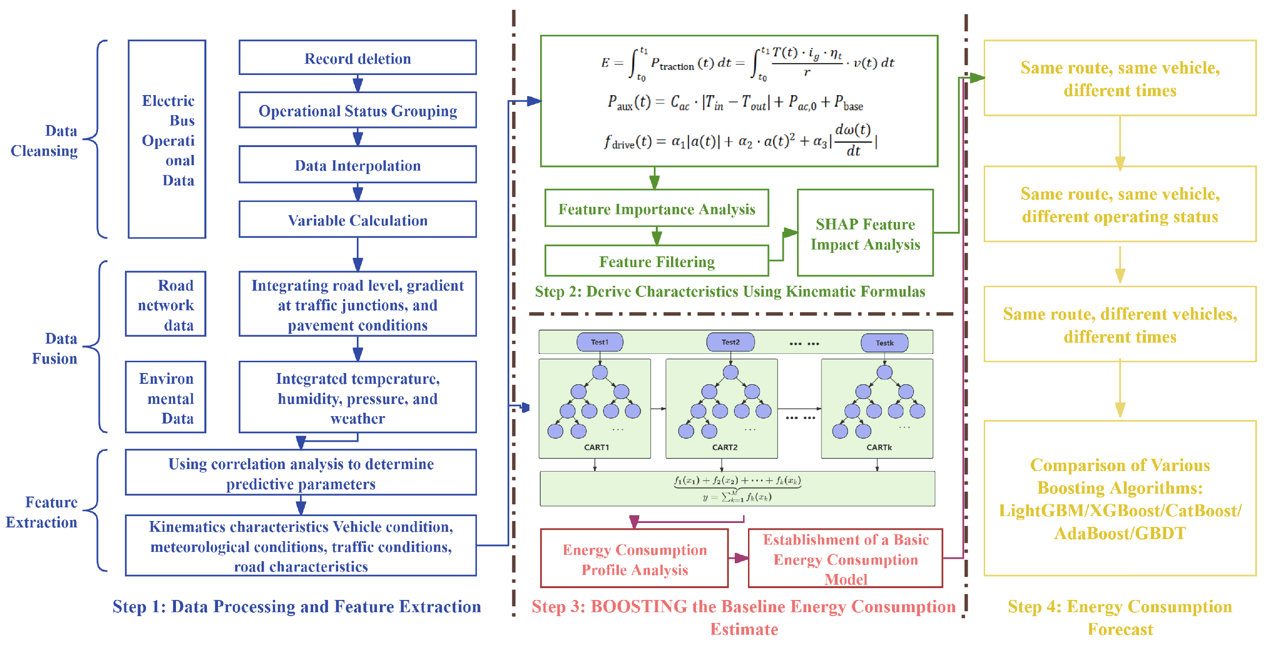
To model this problem, this study integrates physics-based and data-driven approaches. The overall framework consists of four main stages, as illustrated in Figure 1. First, multi-source operational data are preprocessed and relevant features are extracted. Second, a physics-based model is constructed to characterize the fundamental relationships between vehicle dynamics and energy consumption. Third, a data-driven model based on boosting algorithms is trained using the same feature set. Finally, the model performance is evaluated under different operating conditions.

3. Data Acquisition and Processing

3.1. Data Collection

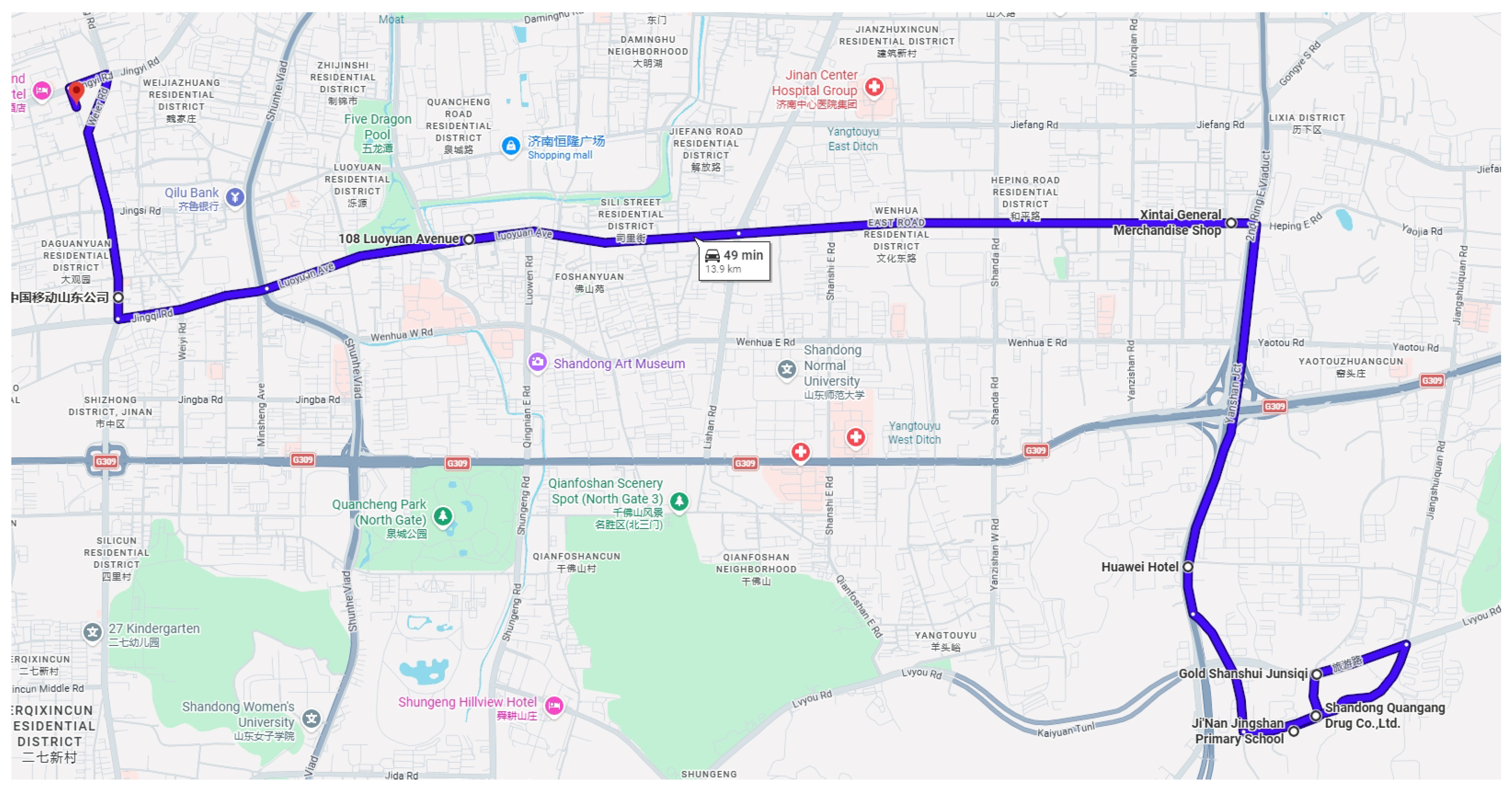
This study focuses on Jinan Bus Route 49, which operates within Jinan’s central urban area (see Figure 2). The route has 29 stops along its 13.5 km length, traversing the east-west arterial roads of the central city. Its operating hours are uniformly set from Monday to Sunday (05:25–21:30), with a headway of approximately 9–16 min. This route deploys 30 buses.

Multi-source operational data—including vehicle trajectory, dynamics, motor, battery, and energy consumption—were collected via the CAN bus at a raw sampling frequency of 5 Hz. The dataset collection spans from December 2023 to January 2024, covering complete all-day operational data for both weekdays and holidays. To reduce computational cost while preserving essential dynamic characteristics, the data were resampled to 1 Hz following common practice in the literature.

Before model construction, the raw data are perprocessed to ensure data quality and consistency. Specifically, remove invalid records (such as zero-position data or missing voltage or current measurements), delete null values, and filter outliers based on physical constraints and data consistency checks. Subsequently, perform time alignment for all variables to ensure synchronization between different data sources. After preprocessing, the final dataset contains approximately 1.2 million samples.

Table 1. Available CAN bus variables and selected features used in the model.

Variable	Description	Source	Used in Model
Speed	Vehicle longitudinal speed	CAN bus	✓
Mileage	Accumulated driving distance	CAN bus	×
Total Voltage	Battery pack voltage	CAN bus	×
Total Current	Battery pack current	CAN bus	✓
Acceleration	Vehicle acceleration	CAN bus	✓
SOC	State of charge of battery	CAN bus	✓
Longitude	Geographic longitude	GPS	×
Latitude	Geographic latitude	GPS	×
Motor Speed	Motor rotational speed	CAN bus	✓
Motor Torque	Motor output torque	CAN bus	✓
Max Cell Voltage	Maximum cell voltage	CAN bus	×
Min Cell Voltage	Minimum cell voltage	CAN bus	×
Max Cell Temp	Maximum cell temperature	CAN bus	×
Min Cell Temp	Minimum cell temperature	CAN bus	×
Outside Temp	Ambient temperature	Sensor	✓
Cabin Temp	Interior temperature	Sensor	✓
Motor Ctrl Voltage	Motor controller voltage	CAN bus	×
Motor Ctrl Current	Motor controller current	CAN bus	✓

summarizes all the variables that can be obtained through the CAN bus. Based on this dataset, key features were selected as model inputs considering the correlation between variables and energy consumption as well as model efficiency.

To preserve temporal dependency and avoid data leakage, a time-based splitting strategy is used. Data from the first two weeks is used for model training, while data from the third week is reserved for model testing. In the training set, 80% of the data is used for model fitting, and 20% of the data is used for validation during the hyperparameter optimization process. This setup ensures a realistic evaluation of the model’s performance under actual operational conditions.

3.2. Data Integration

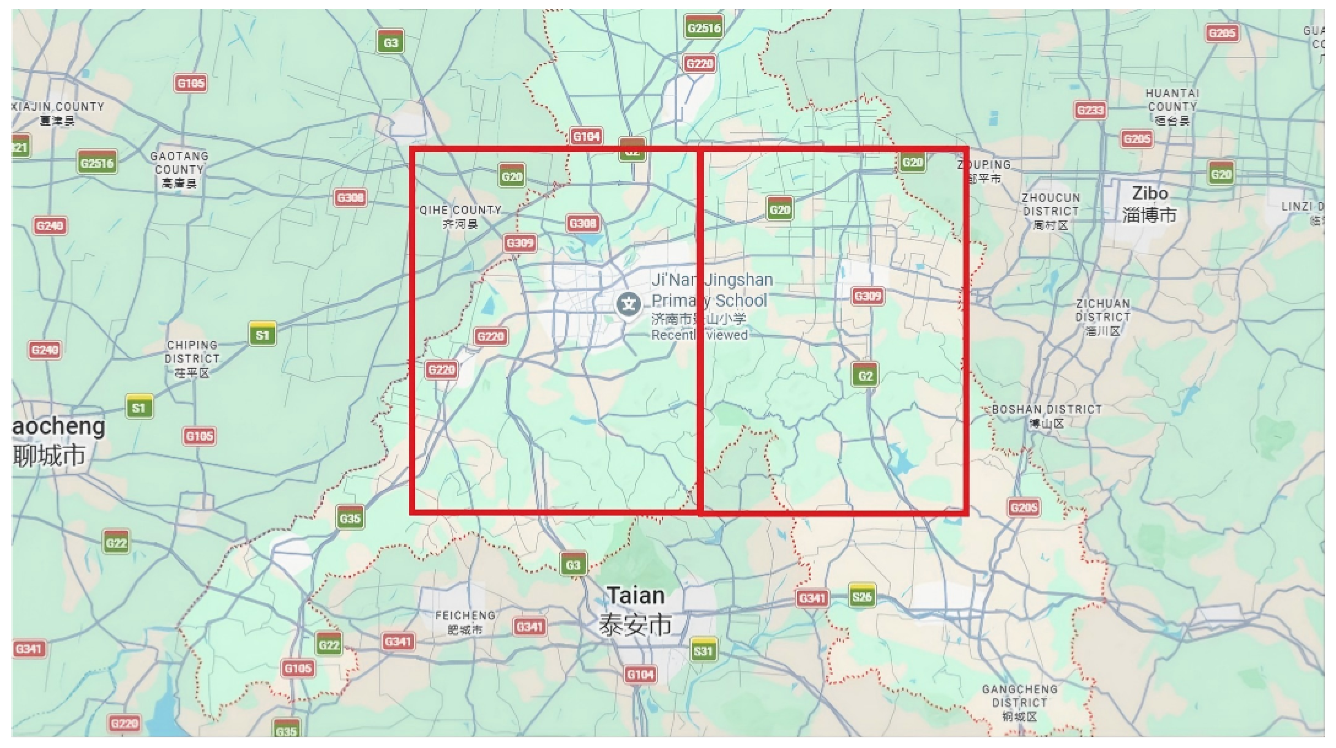
According to relevant research, the energy consumption of vehicles is strongly correlated with road conditions and terrain. Since the location data in the dataset originate from GNSS positioning, and signal drift causes variations in the positioning data for the same road segment. To ensure consistent road gradients and positioning signals for the same road segments, we employ a grid-based mapping approach. This method consolidates the positioning data within each grid cell at a unified grid positioning point. Elevation data is sourced from the Geospatial Data Cloud accessed on 12 November 2025 (https://www.gscloud.cn/search), and we use the GDEMV3 30 m resolution digital elevation data for this study, as illustrated in Figure 3:

The positioning dataset are grouped into grids with a 30 m size, and the corresponding elevation data for each grid is matched synchronously. By calculating the elevation differences between adjacent grids and converting them based on the grid size, we derive the actual road slope. This enables an in-depth integrated analysis of the road topographical conditions and operational data.

Based on the collection dates and times in the operational data and in accordance with typical urban transit patterns, we divide a day into the following periods: late evening off-peak: from the start of service to 6:20 a.m.— Morning peak: 6:20 AM to 8:20 AM—Off-peak: 8:20 AM to 4:00 PM—Evening peak: 4:00 PM to 6:00 PM—late evening off-peak: 6:00 p.m. to the end of service. Based on weekly work patterns, we divide a week into weekdays and rest days. We integrate the operational patterns with the collected data for each category. The daily weather conditions are also integrated into the dataset.

4. Methods for Energy Consumption

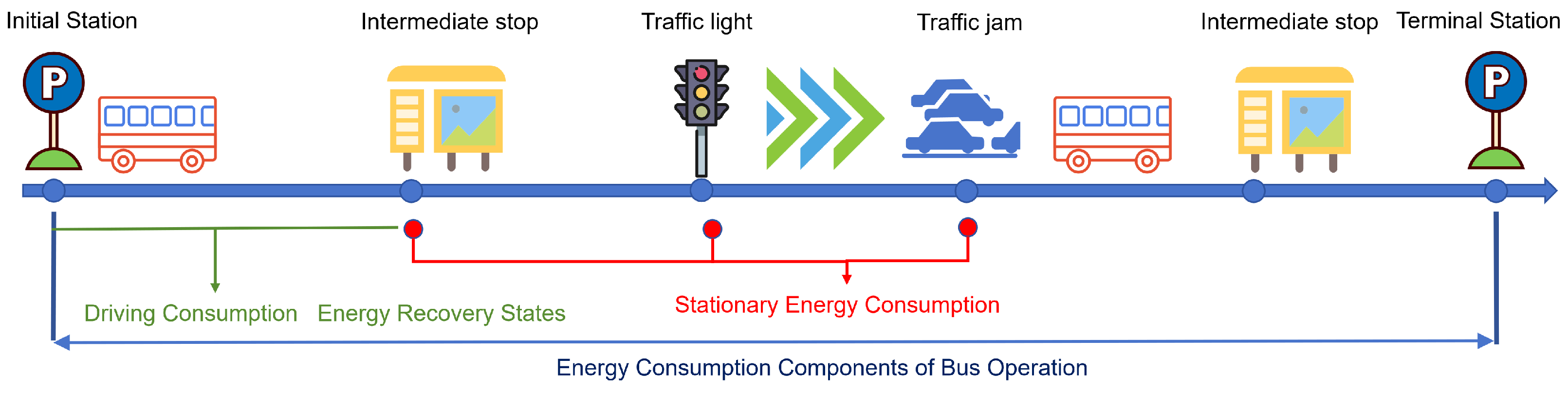
This study analyzes the energy consumption of urban buses during actual operation. Based on vehicle operating conditions, the operational process is categorized into driving mode and stationing mode. Energy consumption during driving mode is further divided into driving consumption and energy recovery states, while energy consumption during stationing mode constitutes stationing energy consumption, as illustrated in Figure 4.

4.1. Physical Energy Consumption Model

In this study, we develop a model for energy consumption under different operating conditions, and analyze the impacts of various factors on energy consumption across different states. Based on research on the factors affecting the energy consumption of electric buses, Al-Wreikat and Liu et al. [18,34] proposed that the energy consumption of electric buses mainly consists of three components: (1) the energy consumed to provide vehicle traction; (2) the energy consumption caused by variations in driver operation during driving; (3) the energy consumed by vehicle accessories (e.g., air conditioning and lighting). Therefore, the comprehensive energy consumption of electric buses can be summarized by Equation (1):

$$E_{\mathrm{Total}}=A_{\mathrm{DSA}}·E_{\mathrm{Traction}}+E_{\mathrm{Accessory}}$$

(1)

$E_{\mathrm{Total}}$: Total energy consumption of the electric bus, in kWh; $E_{\mathrm{Accessory}}$: Accessory energy consumption, which is the energy required to propel the vehicle during operation (determined by motor torque and speed), in kWh; $E_{\mathrm{Traction}}$: Traction energy consumption, which is the energy consumed by on-board equipment (e.g., air conditioning, lighting, and instrument panels), in kWh; $A_{\mathrm{DSA}}$: Driving style adjustment factor, a dimensionless parameter reflecting the energy consumption variation caused by driver habits (e.g., frequent acceleration and deceleration).

4.1.1. Traction Energy Consumption Model

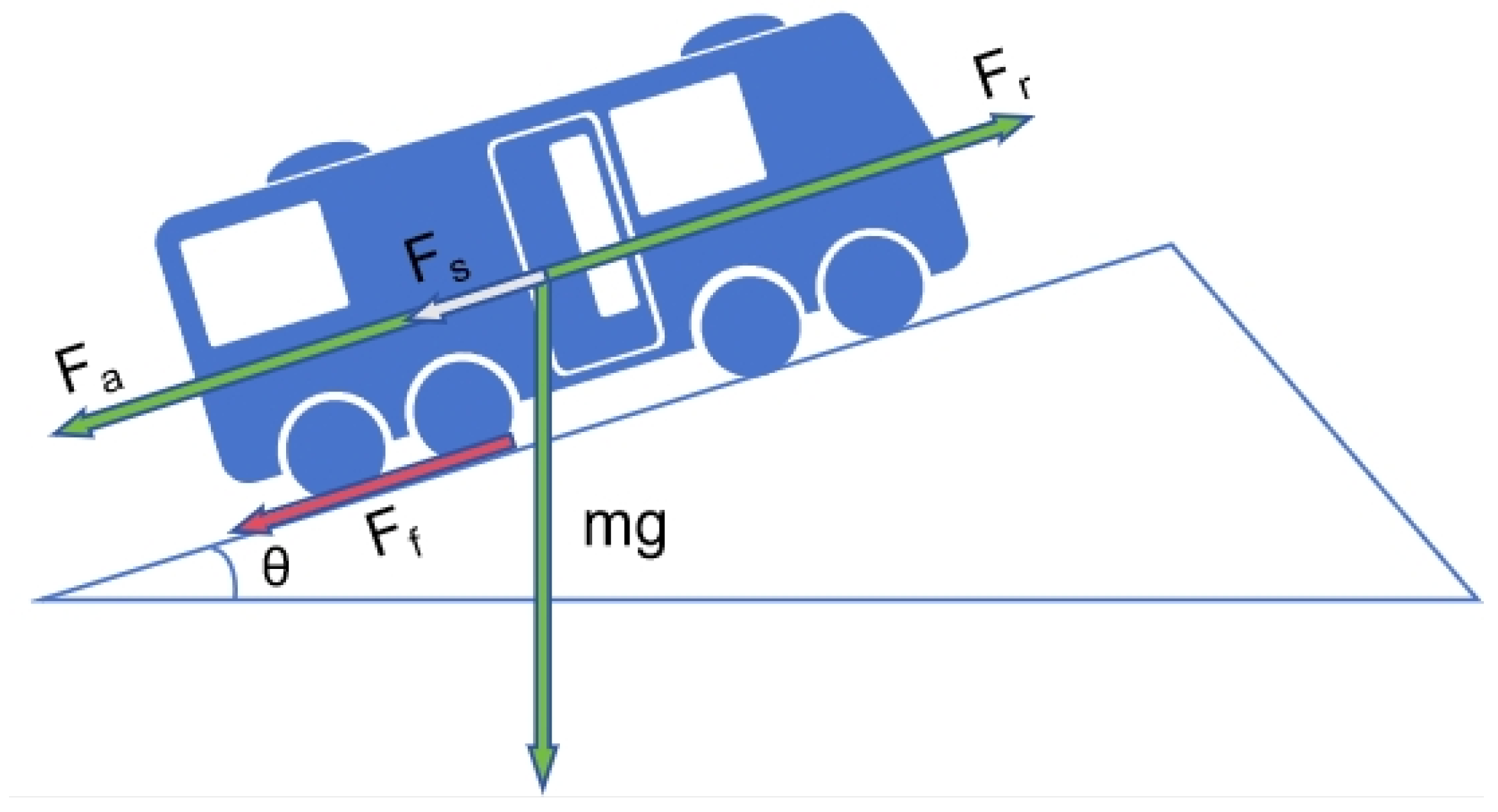
The physical dynamic model of electric vehicles is widely applied to energy consumption calculations [15,35]. By analyzing the forces acting on electric buses during operation, we identify the factors influencing their energy consumption, thus deriving an energy consumption equation for predictive purposes. Based on the vehicle dynamics model, we analyze the forces acting on electric buses during actual operation, as shown in Figure 5.

The energy consumption of electric buses is mainly determined by the resistive forces acting on the vehicle during operation, including rolling resistance, aerodynamic drag, gradient resistance, and acceleration resistance. The equation for the traction force (driving force) of electric buses during operation is given by Equation (2):

$$F_{\mathrm{traction}}=F_{\mathrm{rolling}}+F_{\mathrm{aero}}+F_{\mathrm{slope}}+F_{\mathrm{acc}}$$

(2)

where $c_r$ Rolling resistance coefficient, dimensionless, typically ranging from 0.005 to 0.015. m Mass of the electric bus, in (kg), g denotes gravitational acceleration (9.81 m/s²), $\rho$ is the air density (approximately 1.225 kg/m²), $C_d$ is the air resistance coefficient (typically 0.6 to 0.9 for buses), A is the frontal area (m²), v is the vehicle speed (m/s), i is the road gradient angle, approximated as a gradient percentage when small (for a 5% gradient, i = 0.05), and is the vehicle acceleration (m/s²). Substituting the respective resistance Equations yields the traction force calculation Equation as Equation (3):

$$F_{\mathrm{traction}}=m·a+c_r·m·g+{\displaystyle \frac{1}{2}}·\rho ·C_d·A·v^2+m·g·i$$

(3)

Equation (3) eveals that road angle data are absent from the collected data, thus requiring us to modify the equation. Since torque data are available in the collected data, the relationship between the traction force $F_{\mathrm{traction}}$ of the bus and the torque T output by the drive wheels is as follows. For an electric bus with a single-stage reducer, the traction force can be calculated using Equation (4):

$$F_{\mathrm{traction}}={\displaystyle \frac{T·i_g·{\eta }_t}{r}}$$

(4)

where T is motor output torque (Nm), $i_g$ is Reduction ratio (unitless), typically a known fixed value, ${\eta }_t$ is Transmission system efficiency (generally around 0.9 to 0.95), r is Wheel radius (m), typically a known fixed value.

The vehicle’s traction power is determined by the product of traction force and vehicle speed, which can be expressed as:

$$P_{\mathrm{traction}}=F_{\mathrm{traction}}·v$$

(5)

where $P_{\mathrm{traction}}$ denotes the traction power, $F_{\mathrm{traction}}$ is the total traction force acting on the vehicle, and v represents the vehicle speed.

According to Equations (4) and (5), the instantaneous power required by the vehicle’s motor under a given state is given by Equation (6).

$$P_{\mathrm{traction}}=F_{\mathrm{traction}}·v={\displaystyle \frac{T·i_g·{\eta }_t}{r}}·v$$

(6)

Energy consumption is the integral of power over time, as given by Equation (7).

$$E={\int }_{t_0}^{t_1}{P}_{\mathrm{traction}}\left(t\right)dt={\int }_{t_0}^{t_1}{\displaystyle \frac{T\left(t\right)·i_g·{\eta }_t}{r}}·v\left(t\right)dt$$

(7)

Taking energy recovery into account, the energy consumption of the traction model during regenerative braking is given by Equation (8)

$$E_{\mathrm{regen}}={\eta }_{\mathrm{regen}}·{\int }_{t_0}^{t_1}max\left(0,-P_{\mathrm{traction}}\left(t\right)\right)dt$$

(8)

where ${\eta }_{\mathrm{regen}}$ is the regenerative braking efficiency (typically 0.6–0.8), and $P_{\mathrm{traction}}\left(t\right)$ is negative during braking.

4.1.2. Driving Correction Model Power

The impact of driving style on energy consumption can be characterized by acceleration, speed fluctuations, and motor speed variations [35]. A driving style influence factor $f_{\mathrm{drive}}\left(t\right)$ is typically defined by combining the absolute value of acceleration, the square of acceleration, and motor speed fluctuations, as given by Equation (9):

$$f_{\mathrm{drive}}\left(t\right)=a_1\left|a\left(t\right)\right|+a_2·a{\left(t\right)}^2+a_3\left|{\displaystyle \frac{d\omega \left(t\right)}{dt}}\right|$$

(9)

where $a_1,a_2,a_3$: Fitting coefficients, determined by historical operational data, $a\left(t\right):$ Vehicle acceleration, in (m/s²), $\omega \left(t\right)$: Motor rotational speed, in (rad/s).

This factor serves as a correction factor for traction power. Based on Equations (6) and (9), the energy consumption model incorporating driving style corrections is derived as Equation (10):

$$P_{\mathrm{traction}}^{\prime }\left(t\right)=f_{\mathrm{drive}}\left(t\right)·{\displaystyle \frac{T\left(t\right)·i_g·{\eta }_t}{r}}·v\left(t\right)$$

(10)

4.1.3. Vehicle Basic Energy Consumption

The baseline energy consumption of a vehicle refers to the power consumption of on-board air conditioning and other auxiliary equipment (e.g., lighting and control systems), which typically constitutes a continuous load as Equation (11).

$$P_{\mathrm{aux}}\left(t\right)=P_{\mathrm{AC}}\left(t\right)+P_{\mathrm{base}}$$

(11)

where $P_{\mathrm{aux}}\left(t\right)$: Instantaneous auxiliary power consumption, in KW; $P_{\mathrm{AC}}\left(t\right)$ Instantaneous air conditioning power consumption, in KW; $P_{\mathrm{base}}$ Baseline power consumption of on-board electronic equipment, in KW; Highly temperature-dependent, can be represented by a temperature-difference-related function as Equation (12).

$$P_{\mathrm{AC}}\left(t\right)=C_{\mathrm{ac}}·|\Delta T|+P_{\mathrm{ac},0}$$

(12)

The temperature difference between the inside and outside of the car is $\Delta T=|T_{\mathrm{in}}-T_{\mathrm{out}}|$, where $T_{\mathrm{in}}$ Cabin temperature, in °C; $T_{\mathrm{out}}$ Ambient temperature, in °C; $C_{\mathrm{ac}}$: Air conditioning power-temperature coefficient, in KW/°C; $P_{\mathrm{ac},0}$: Air conditioning baseline standby power, in KW.

The comprehensive equation for baseline accessory energy consumption is given by Equation (13):

$$P_{\mathrm{aux}}\left(t\right)=C_{\mathrm{ac}}·|T_{\mathrm{in}}-T_{\mathrm{out}}|+P_{\mathrm{ac},0}+P_{\mathrm{base}}$$

(13)

4.1.4. Comprehensive Energy Consumption Model Equation

By integrating all the above components according to Equations (1), (10) and (13), we obtain the following:

Instantaneous total power equation (accounting for driving style, air conditioning, and baseline energy consumption) as Equation (14):

$$P_{\mathrm{total}}\left(t\right)=f_{\mathrm{drive}}\left(t\right)·{\displaystyle \frac{T\left(t\right)·i_g·{\eta }_t}{r}}·v\left(t\right)+P_{\mathrm{aux}}\left(t\right)$$

(14)

According to Equations (1), (10) and (13) the physical driving model requires the following parameters to calculate the energy consumption of electric buses, as presented in

Table 2. Physical driving dynamics model parameters.

Type	Name	Symbol	Unit	Source
Vehicle Physical Data	Speed Ratio	$i_g$	-	Vehicle Physical Parameters
	Transmission System Efficiency	${\eta }_t$	-
	Wheel Radius	r	m
Vehicle Driving Data	Speed	v	m/s	CAN Data
	Torque	T	Nm
	Acceleration	a	${\mathrm{m}/\mathrm{s}}^2$
	Motor Speed	$\omega$	rad/s
	Cabin Temperature	$T_{in}$	°C
	Ambient Temperature	$T_{out}$	°C
Fitting Coefficient Data	Fitting Coefficient	${\alpha }_1,{\alpha }_2,{\alpha }_3$	-	Model Fitting
	Base Energy Consumption	$P_{base}$	-
	Air Conditioning Temperature Coefficient	$C_{ac}$	-
	Air Conditioning Power	$P_{ac,0}$	-
Predictive Data	Power	P	kW	CAN Data

:

4.2. Data-Driven Energy Consumption Enhancement Model

Physics-based energy consumption models provide transparency and physical interpretability, but their predictive performance deteriorates under the complex and highly variable operating conditions common in urban bus operations (e.g., stop-and-go traffic, regenerative braking, passenger load fluctuations, and frequent changes in auxiliary power demand). To overcome these limitations, this study adopts a data-driven approach for instantaneous electric bus energy consumption prediction using real-world operational data.

The data-driven prediction problem addressed in this study has two key characteristics that directly determine the selection of the modeling approach:

(1) strong nonlinearity and feature interaction effects.

Electric bus energy consumption depends on complex, nonlinear interactions among vehicle dynamics (e.g., torque, speed, acceleration), powertrain behavior, and environmental conditions. These interactions are difficult to represent using parametric models or linear regression, particularly at high temporal resolution. Tree-based ensemble methods can naturally capture such nonlinearities and interaction effects without requiring explicit functional assumptions or extensive feature engineering.

(2) Practical constraints of real-world public transport data and applications.

Operational data collected from the CAN bus systems are heterogeneous and noisy, and are often limited to a set of sensor variables that vary across vehicle types and fleets. For public transport applications, prediction models must be robust to missing or imperfect data, computationally efficient, and easy to deploy for planning and operational decision support. Compared with deep learning approaches, ensemble tree-based models require less data preprocessing, exhibit greater training stability, and provide strong performance on structured tabular data commonly available to transit agencies.

Given these characteristics, this study adopts Boosting-based ensemble learning methods for data-driven energy consumption prediction. Boosting algorithms iteratively combine multiple weak learners by assigning higher weights to samples that are difficult to predict, thereby enabling the model to progressively learn fine-grained patterns in complex operational data. This makes boosting particularly effective for regression problems involving high-frequency vehicle operation data.

Five representative Boosting algorithms are selected for this study: AdaBoost, Gradient Boosting Decision Trees (GBDT), XGBoost, LightGBM, and CatBoost. These methods differ in their tree construction strategies, regularization mechanisms, and computational efficiency, thus enabling a systematic comparison of their predictive performance and generalization ability under consistent input features derived from the physical energy consumption model.

To further ensure the physical consistency of the data-driven model, this paper employs a discrete integration method based on predicted power to estimate total energy consumption. In addition to outputting instantaneous power predictions, the model can also estimate total energy consumption by performing discrete integration over the time domain. Specifically, the formula for calculating energy consumption is as Equation (15):

$$E_{\mathrm{trip}}=\sum _{k=1}^N{P}_k·\Delta t={\displaystyle \frac{1}{f_s}}\sum _{k=1}^N{P}_k$$

(15)

where $E_{\mathrm{trip}}$ represents the total energy consumption per trip, $P_k$ represents the predicted instantaneous power at the k time step, $\Delta t$ represents the time step size, $f_s$ represents the data sampling frequency, and N represents the total number of time steps in the trip. By summing the instantaneous power over time, this method links the model’s instantaneous predictions to macro-level energy consumption metrics, thereby effectively validating the model’s physical plausibility.

To enhance model interpretability and ensure consistency with physical mechanisms, we apply SHAP (SHapley Additive exPlanations) analysis to the selected Boosting model. This enables a quantitative assessment of the contribution of individual features to the predicted energy consumption and facilitates meaningful interpretation for public transport operators and planners.

4.3. Model Implementation and Hyperparameter Optimisation

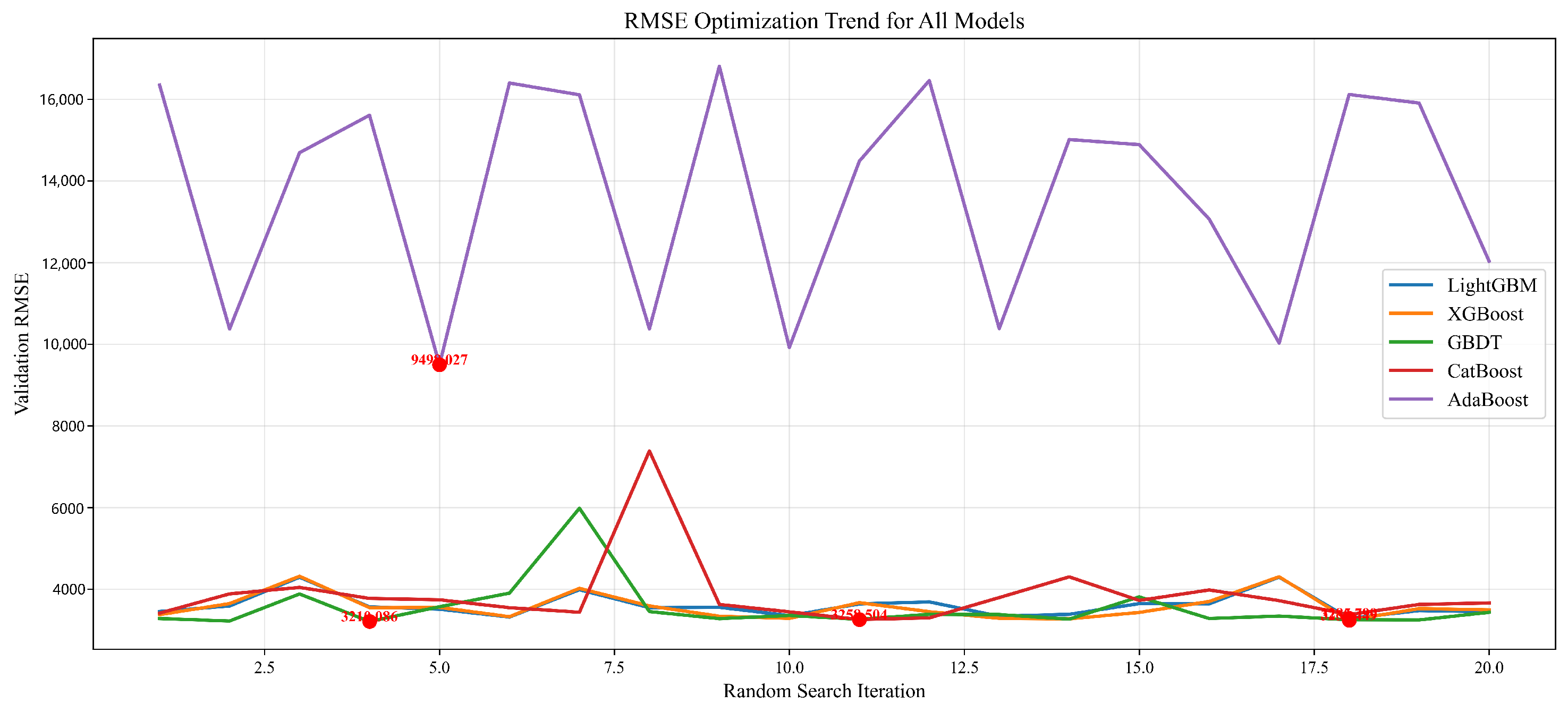
To ensure fair comparison and optimal performance, all boosting models were tuned using a random search strategy. The hyperparameter search spaces were defined based on prior studies, including the number of trees (100–1000), learning rate (0.01–0.2), maximum depth (3–10), subsampling ratio (0.6–1.0), and regularization parameters (L1 and L2: 0–10) for XGBoost and LightGBM. For CatBoost, depth (4–10), learning rate (0.01–0.2), and iterations (200–1000) were optimized, while for AdaBoost, the number of estimators (50–500) and learning rate (0.01–1) were considered. Random search was adopted due to its efficiency in exploring high-dimensional parameter spaces. All models were trained on the same dataset, and the optimal hyperparameters were selected by minimizing the root mean square error (RMSE) on the validation set, as shown in the Figure 6. The models were implemented in Python 8.0 and trained on a workstation with an Intel i7 CPU (3.4 GHz) and 64 GB RAM.

The optimal hyperparameters are summarized in

Table 3. Optimal hyperparameters for different models obtained random search.

Model	Learning Rate	Max Depth	Estimators	Subsample	L1	L2
LightGBM	0.122	8	646	0.885	4.722	1.196
XGBoost	0.122	8	646	0.885	4.722	1.196
GBDT	0.134	7	869	0.889	–	–
CatBoost	0.127	9	886	–	–	–
AdaBoost	0.068	–	137	–	–	–

. In general, the models favor moderate learning rates (approximately 0.07–0.13) and relatively deep trees (depth 7–9), indicating the strong nonlinear characteristics of the energy consumption process. In particular, LightGBM and XGBoost exhibit nearly identical optimal configurations, suggesting that both models capture similar underlying data structures, while CatBoost tends to adopt deeper trees and more iterations to achieve comparable performance. These findings further support the suitability of tree-based ensemble methods for modeling complex, high-frequency operational data.

5. Results and Discussion

To ensure the reliability of the evaluation and account for time-dependent characteristics, all models in this section employ time-series splitting: data from the first two weeks are used for training, while data from the third week serve as the test set to simulate predictions for unknown future data. This strategy avoids information leakage caused by random splitting and ensures that the results accurately reflect the model’s generalization performance in real-world scenarios. Subsequent residual analysis, prediction interval estimation, and statistical significance tests are all conducted exclusively on this test set to ensure the consistency and reliability of the conclusions.

5.1. Comparison of Predictions Across Different Models

To control for confounding factors and ensure a fair comparison, this study utilizes actual operational data from Jinan’s Route 49 electric bus (license plate number 22031031). Within the time-segmentation framework, the model is trained on data from the first two weeks and tested on data from the third week, with representative subsets of the test set selected for analysis and visualization. Input variables are derived from the physical model Equations (9), (12) and (13), including speed, acceleration, torque, motor speed, cabin temperature, and ambient temperature; the output variable is instantaneous power. This paper compares two types of methods—physics-driven and data-driven—analyzing prediction accuracy and performance under a unified data and evaluation framework to validate their effectiveness in modeling complex bus scenarios.

5.1.1. Physical Model Prediction

Using the torque-based energy consumption physical model as Equation (14), the instantaneous energy consumption of the electric bus is set as the output, with speed, acceleration, torque, motor speed, cabin temperature, and ambient temperature as the inputs. The parameter values are set as $i_g=2.5$, ${\eta }_t=0.9$ and $r=0.635$ m for model fitting. The fitted parameters obtained are as follows: $a_1=186.516753$, $a_2=-90.367503$, $a_3=80.193313$, $C_{\mathrm{ac}}=3.396024$, $P_{\mathrm{ac},0}=3.419866$, $P_{\mathrm{base}}=0.872529$.

$$\left\{\begin{array}{cc}\hfill f_{\mathrm{drive}}\left(t\right)& =186.51a\left(t\right)-90.37·\left(a{\left(t\right)}^2+80.19·{\displaystyle \frac{dw\left(t\right)}{dt}}\right)\hfill \\ \hfill P_{\mathrm{friction}}\left(t\right)& =f_{\mathrm{drive}}\left(t\right)·3.543·T\left(t\right)·v\left(t\right)\hfill \\ \hfill P_{\mathrm{aux}}\left(t\right)& =11.58·|T_{\mathrm{in}}-T_{\mathrm{out}}|+0.873\hfill \end{array}\right.$$

Substituting the relevant parameters into Equation (14), a physics-based instantaneous energy consumption model is constructed. To ensure a consistent and fair comparison with the machine learning frameworks, this model is evaluated using the identical high-resolution dataset. While the physics-based model achieves a moderate coefficient of determination ($R^2\approx 0.734$) during routine operations by effectively utilizing kinematic and thermal features, its predictive capability diminishes significantly under specific operating modes. As detailed in

Table 4. Physical Driving Model Evaluation Metrics.

Data Types	Model Evaluation
	RMSE	MAE	MAPE (%)	${\mathit{R}}^{\mathbf{2}}$
Energy Consumption Data	14.295	10.942	157.63	0.7349
Energy Recovery	14.59	11.15	279.93	0.214
Stationary Energy Consumption	3.43	2.74	117.45	0.176

, the $R^2$ values drop to approximately 0.20 and 0.17 for the energy recovery and stationary states, respectively. This performance degradation is expected and highlights the inherent limitations of simplified physical modeling. In the energy recovery state, the underlying energy dynamics are governed by complex electromechanical coupling and non-linear braking strategies that transcend the assumptions of a linear physics model. Similarly, during stationary periods, energy consumption is dominated by auxiliary systems—such as HVAC and air compressors—which are functionally decoupled from the vehicle’s kinematic variables. Consequently, the deterministic and linear nature of the physics-based approach fails to capture these latent non-linear patterns, whereas the boosting-based models can implicitly learn these relationships from the rich feature set.

5.1.2. Boosting Model Prediction

To more accurately characterize the complex energy consumption variation patterns under dynamic operating conditions, we adopt a data-driven approach for energy consumption prediction. Since data-driven methods are typically considered black-box models, we first analyze the influence of input features on the model’s prediction results. To more accurately and efficiently characterize instantaneous energy consumption changes under different operating power conditions, multiple Boosting algorithms are employed for energy consumption prediction. Model training is performed using the same set of influencing features from the same dataset, and the prediction results of different algorithms are systematically compared. The three-week operational dataset from the same single vehicle is selected: the first two weeks serve as the training set, while the third week constitutes the test set. The training and test metrics for the selected models are presented in

Table 5. Training and testing metrics of each algorithm.

Model	Training Subset				Testing Subset
	RMSE	MAE	MAPE	${\mathit{R}}^{\mathbf{2}}$	RMSE	MAE	MAPE	${\mathit{R}}^{\mathbf{2}}$
LightGBM	3.292	2.336	48.984	0.9903	6.188	4.644	91.02	0.9591
XGBoost	2.997	2.126	45.837	0.992	6.41	4.811	92.86	0.9561
CatBoost	3.396	2.439	51.696	0.9897	6.418	4.711	78.88	0.9560
AdaBoost	10.501	8.726	226.69	0.9015	12.23	10.3	196.41	0.8402
GBDT	2.975	2.126	46.618	0.9921	6.488	4.851	98.07	0.9556

.

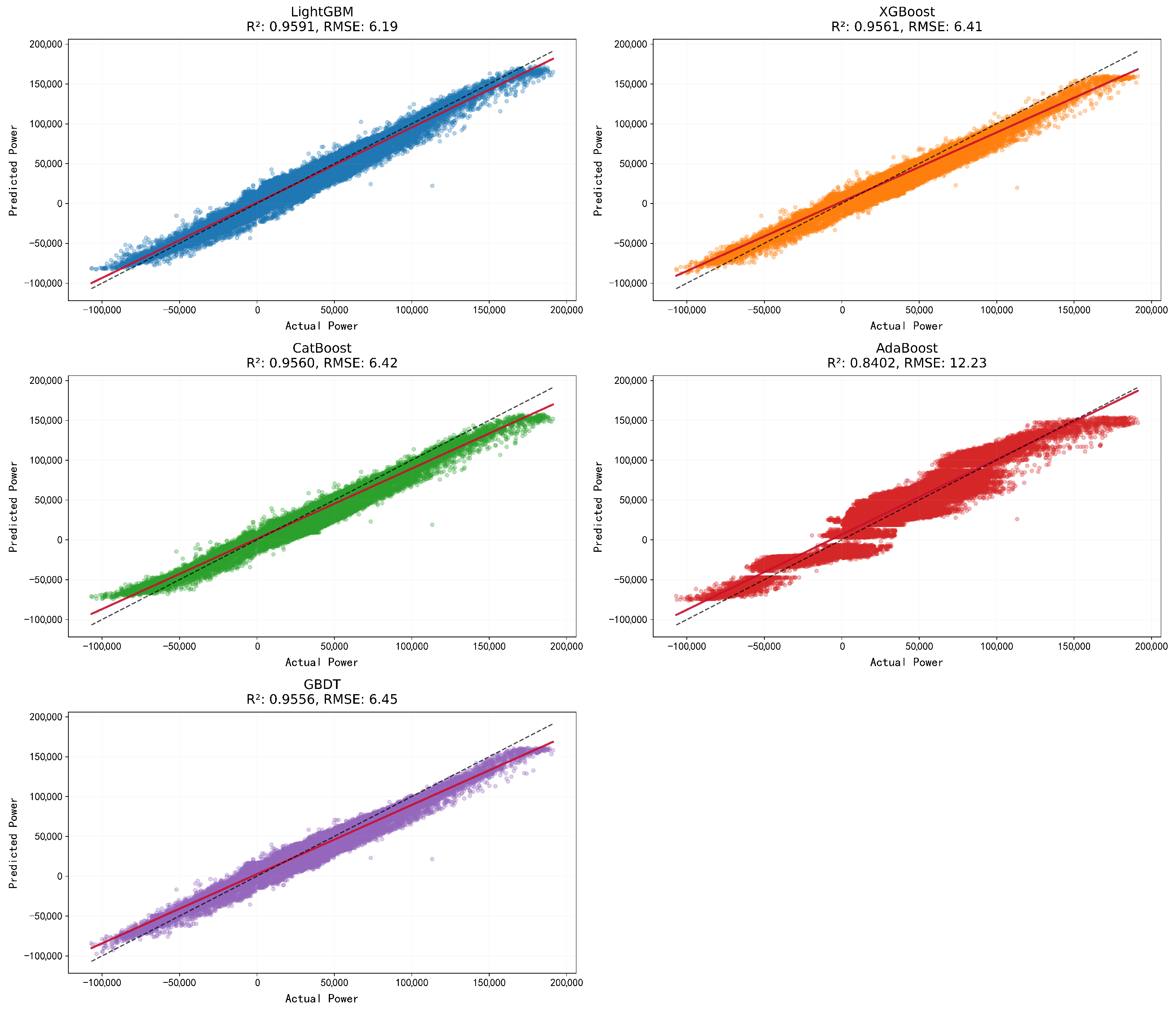
As shown in Table 5, all boosting models except AdaBoost achieve strong predictive performance. On the training set, the models reach an $R^2$ of approximately 0.99 with an RMSE of about 3.2 kW, indicating excellent fitting capability. On the test set, the performance slightly decreases to an $R^2$ of approximately 0.95 with an RMSE of about 6.2 kW, which reflects good generalization ability without significant overfitting.

To provide a more physically meaningful interpretation of the prediction error, the average power is computed using the mean absolute power, which avoids cancellation effects between traction (positive) and regenerative (negative) power. In this study, the mean absolute power is approximately 26.7 kW. Therefore, the test RMSE of 6.2 kW corresponds to roughly 23.2% of the typical power magnitude, indicating that the model maintains reasonable accuracy under real-world operating conditions. It should be noted that MAPE is not a reliable metric in this study due to the presence of both positive (traction) and negative (regenerative) power values, as well as values close to zero, which can lead to inflated percentage errors. Therefore, RMSE and MAE are considered more appropriate evaluation metrics for this task.

As shown in Figure 7, this paper uses scatter plots to analyze the correlation between the predicted values of each algorithm and the actual values, thereby quantitatively evaluating the models’ predictive accuracy. The scatter plot results show that the AdaBoost model’s predictive accuracy is significantly lower, with its data points clearly deviating from the 1:1 reference line; in contrast, the predicted data points for the other four boosting algorithms are highly concentrated near the reference line, demonstrating good predictive accuracy. It is worth noting that the AdaBoost model performs significantly worse than the other boosting algorithms; this result is closely related to its own learning mechanism and sensitivity to noise. The core learning logic of AdaBoost involves continuously increasing the weight of samples with larger errors; this mechanism makes it prone to overfitting when dealing with noisy data. In this study, the high-frequency CAN bus data not only contains measurement noise but also involves complex and irregular operating conditions such as regenerative braking and vehicle standstill. This further causes the AdaBoost model to overemphasize noisy samples, ultimately significantly reducing the model’s generalization performance. In contrast, GBDT, XGBoost, LightGBM, and CatBoost are all built on the gradient boosting framework. Their training process focuses on fitting model residuals rather than reweighting samples. This characteristic makes them more robust to data noise and better able to accurately capture the strong nonlinear relationships present in electric bus energy consumption data. In summary, the AdaBoost model performed poorly in the energy consumption prediction task of this study, primarily due to its high sensitivity to noise and limited ability to model complex nonlinear dynamics. In contrast, the other gradient boosting algorithms demonstrated superior predictive performance in this task thanks to their more suitable learning mechanisms.

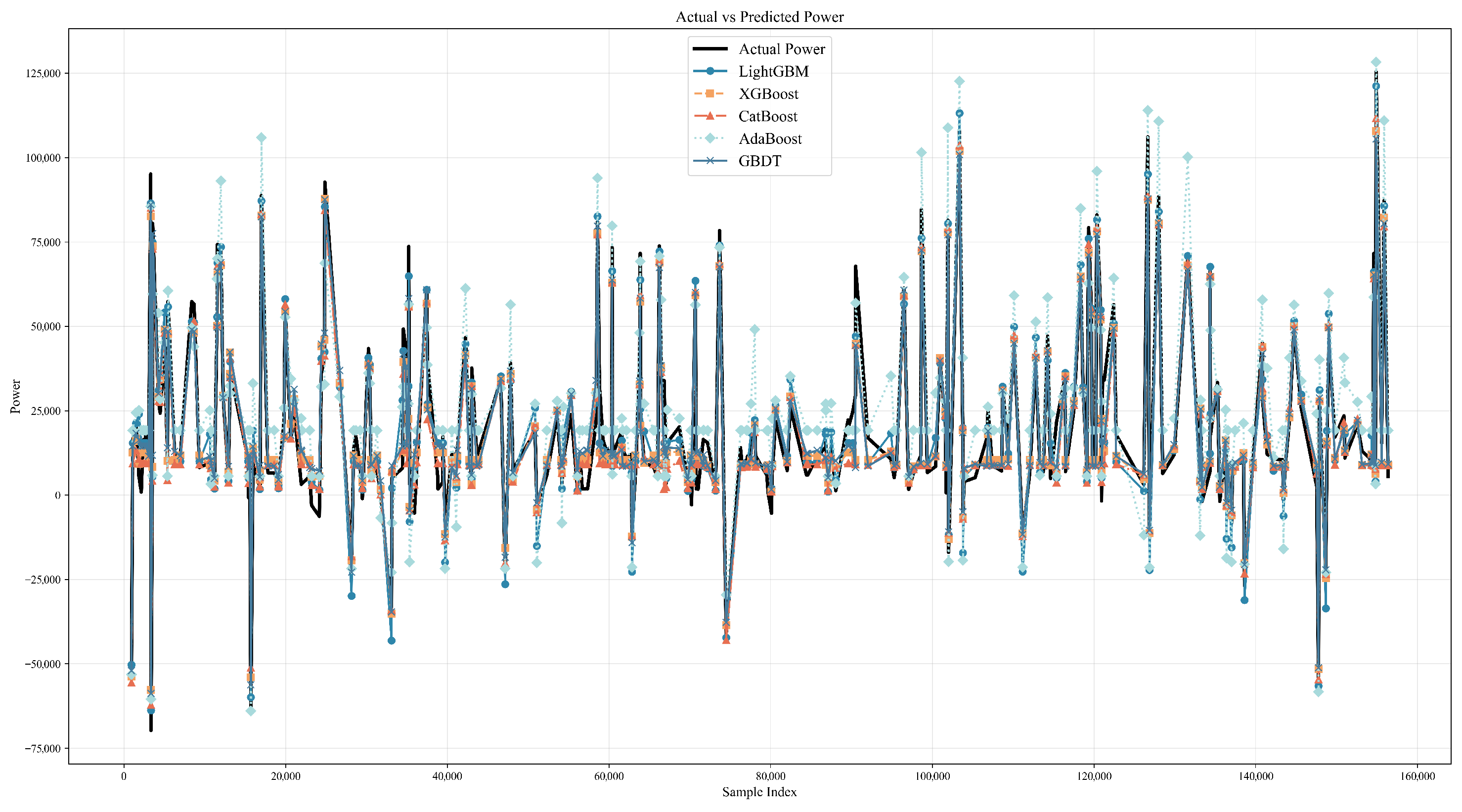
As shown in Figure 8, a comparison of the prediction results using the same test data shows that all algorithms except AdaBoost demonstrate excellent explanatory power, capturing approximately 95% of the variance on the test set ($R^2\approx 0.95$), while achieving around 99% on the training set. Considering both the training loss curve and prediction stability, CatBoost achieves the best overall balance between accuracy and stability, while XGBoost achieves the lowest prediction error. While XGBoost and GBDT achieve the highest prediction accuracy, GBDT requires a significantly longer training time compared with XGBoost and the other algorithms, and no obvious overfitting is observed in either model.

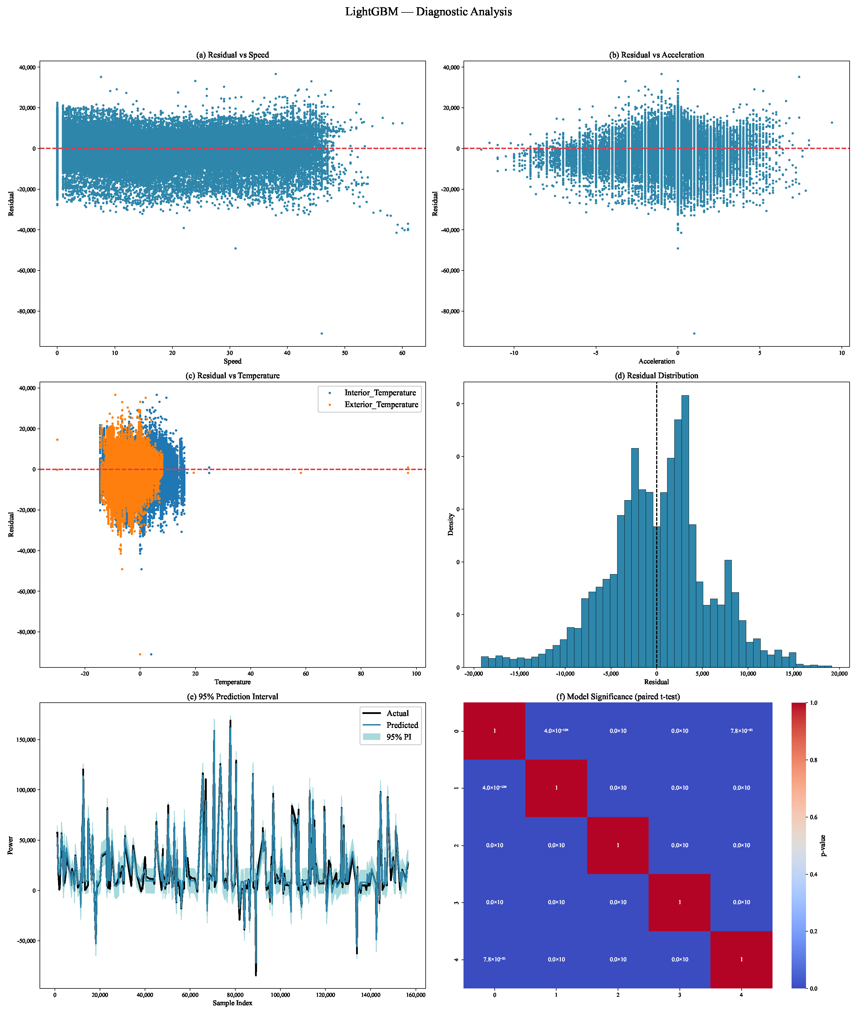
To further evaluate the robustness of the proposed model, a residual analysis was conducted on key operational variables such as vehicle speed, acceleration, and ambient temperature. As shown in Figure 9a–c, the residuals exhibit a random distribution around the zero point, with no obvious systematic trends or patterns of bias. This indicates that the model demonstrates good stability under various vehicle operating conditions and does not exhibit significant systematic prediction bias.

The residual distribution histogram shown in Figure 9d exhibits a symmetric distribution centered at zero, with a distribution shape close to a normal distribution. This further verifies the unbiased nature of the model’s prediction errors, indicating that the model’s prediction results are highly reliable.

In addition to point prediction accuracy, prediction intervals are used to quantify the uncertainty of the model. Prediction intervals are constructed based on the distribution of the residuals. Assuming that the residuals approximately follow a normal distribution, the prediction interval can be estimated as (Equation (16)):

$$\widehat{y}\pm z_{\alpha /2}·\sqrt{\mathrm{MSE}+{\sigma }_{\mathrm{model}}^2}$$

(16)

where $\widehat{y}$ Model prediction, $z_{\alpha /2}$ Quantile of the standard normal distribution at a confidence level of $1-\alpha$ (e.g., 95% confidence level corresponds to $z_{0.025}=1.96$), MSE: Mean Squared Error of the model, ${\sigma }_{\mathrm{model}}^2$ Variance of the model’s inherent uncertainty.

As shown in Figure 9e, the vast majority of actual power values fall within the 95% prediction interval. This indicates that the proposed model effectively captures prediction uncertainty and provides reliable estimates of power values and their associated error bounds. This capability is particularly important for practical engineering applications, as it not only enables accurate predictions but also allows for confidence-based assessments of energy consumption.

To quantitatively verify the performance differences between the proposed model and the baseline models, a paired t-test was employed for statistical significance analysis. As shown in Figure 9f, the p-values from the paired t-tests between the models are all less than 0.01, indicating that the performance differences between the proposed enhanced model and each baseline model are statistically significant. This fully confirms the superiority and effectiveness of the proposed method in power forecasting tasks. These results confirm the robustness, reliability, and statistical validity of the proposed model under time-based evaluation.

Furthermore, since the dataset used in this study was collected from real-world vehicle CAN bus data, it inherently contains measurement noise and sensor uncertainties; both model training and evaluation were conducted under these real-world noise conditions. The model’s residual distribution remained stable and its predictive performance consistent across different operating variables, indicating that the proposed model is insensitive to measurement errors and exhibits excellent robustness in practical applications.

5.1.3. SHAP Analysis of the Boosting Model

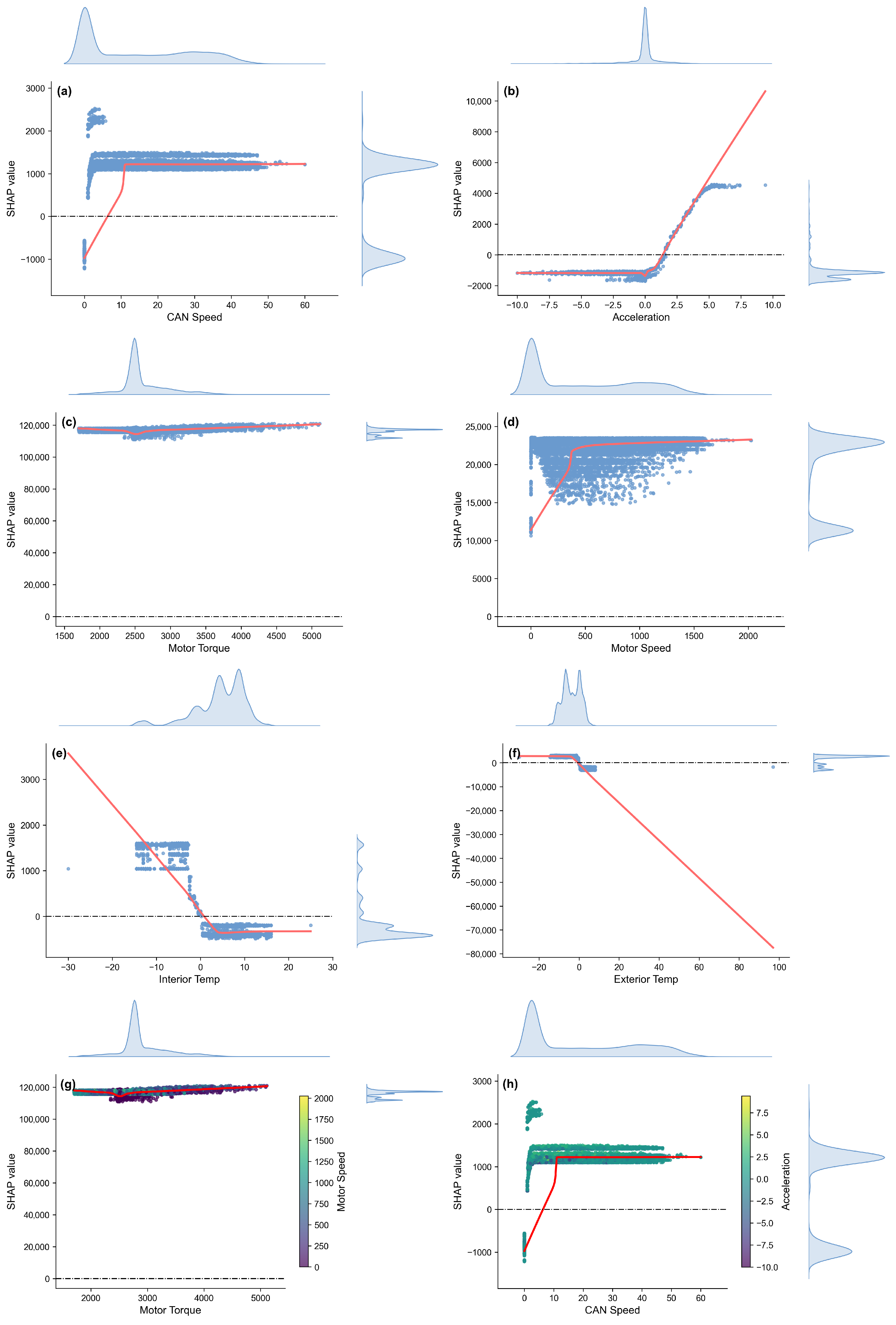
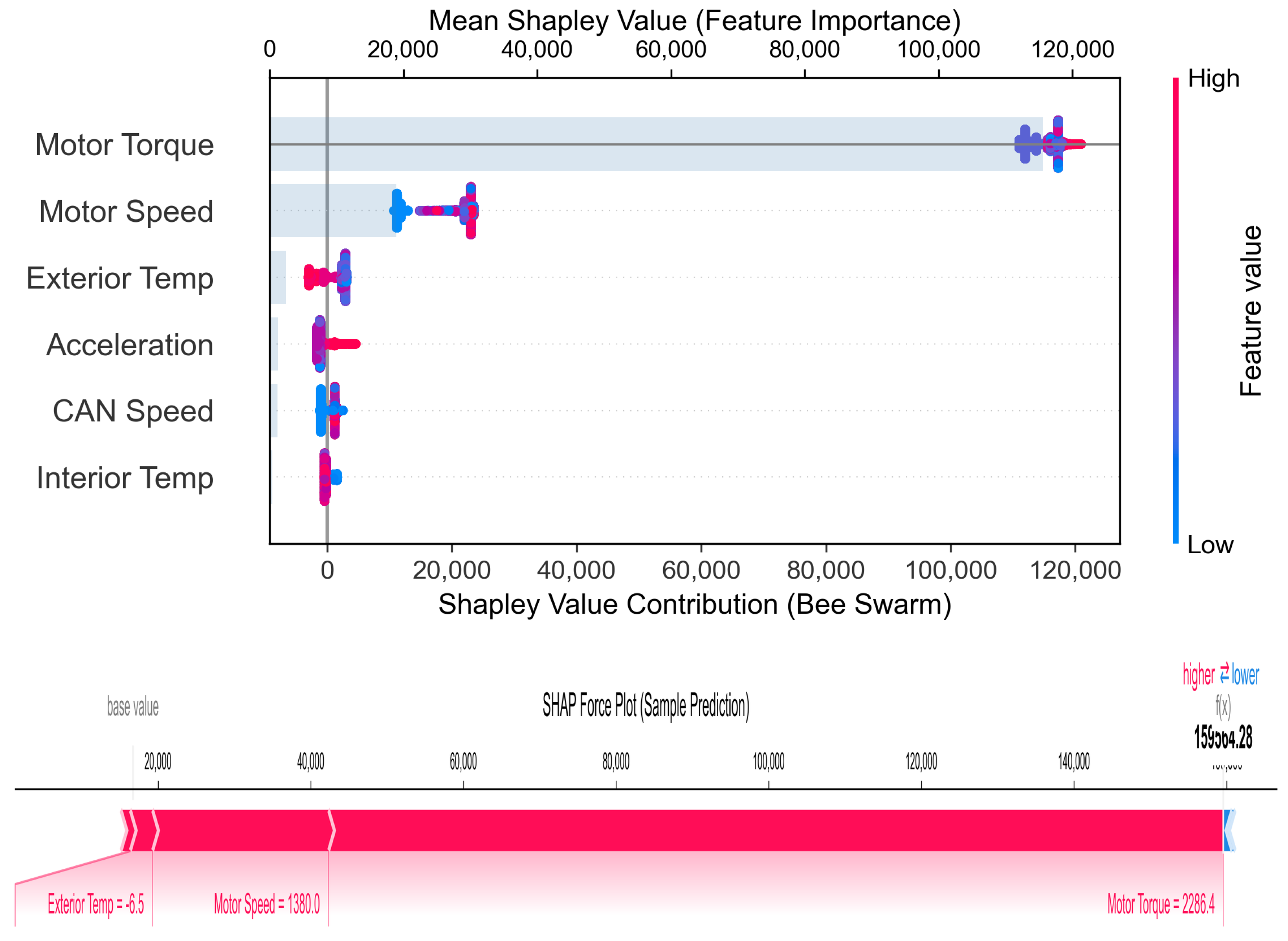
To identify the mechanisms by which each feature contributes to energy consumption prediction and to verify the physical plausibility of the model, the best-performing XGBoost model was selected through comparison and screening based on the existing dataset. A SHAP analysis was then conducted on this model to elucidate the influence patterns of six key features—vehicle speed, acceleration, motor torque, motor speed, interior temperature, and exterior temperature—on instantaneous energy consumption. The SHAP analysis quantified the overall impact of each feature on the model’s prediction results. The ranking of feature importance (based on the average absolute Sharpli value) was as follows: motor torque, motor speed, external temperature, acceleration, CAN bus rate, and interior temperature. Among these, motor torque had the most significant impact, while interior temperature had the least.

The specific mechanisms of these features are as follows: Motor torque makes a strong, stable, and positive contribution to the predicted power (Figure 10c,g). The SHAP value increases monotonically with motor torque, consistent with the physical relationship between torque and output power in electric drive systems, confirming that higher torque demands directly increase energy consumption; Motor speed also exhibits a significant positive contribution (Figure 10d), with SHAP values rising rapidly in the low-speed range and tending toward saturation at high speeds. This reflects the combined effects of transmission system efficiency and rotational losses, demonstrating that the model captures the nonlinear relationship between the two. Acceleration exerts an asymmetric influence on power prediction (Figure 10b): positive acceleration causes the SHAP value to rise sharply (as power demand increases during acceleration), while negative acceleration (deceleration) contributes negatively, consistent with the physical behavior of regenerative braking; Vehicle speed contributes nonlinearly (Figure 10a,h): the SHAP value increases with speed in the low-to-medium speed range and stabilizes at high speeds, corresponding to the pattern of aerodynamic drag variation with speed.

The effects of temperature-related variables have clear physical significance: the SHAP value decreases as the interior temperature rises (Figure 10e), indicating that heating at low temperatures increases additional energy consumption; external temperature shows a significant negative correlation with the SHAP value (Figure 10f), indicating that low ambient temperatures increase energy demand due to HVAC system operation. Furthermore, the SHAP plot (Figure 11) shows that motor torque plays a dominant role in a single prediction, while motor speed and temperature variables provide auxiliary adjustments, reflecting the combined influence of mechanical and environmental factors.

In summary, the SHAP analysis results are highly consistent with established physical principles of vehicle energy consumption, indicating that the proposed model not only possesses high predictive accuracy but also accurately captures the interpretable relationship between input variables and power demand. This confirms that it is not a purely “black-box” model, but rather a physically consistent and interpretable data-driven framework.

5.2. Model Performance Diagnostics

We generate new test datasets by stratifying the original data according to traffic flow periods, sample sizes, and vehicle fleets of different sizes to evaluate the model’s performance under different operating conditions.

5.2.1. Impact of Time Periods

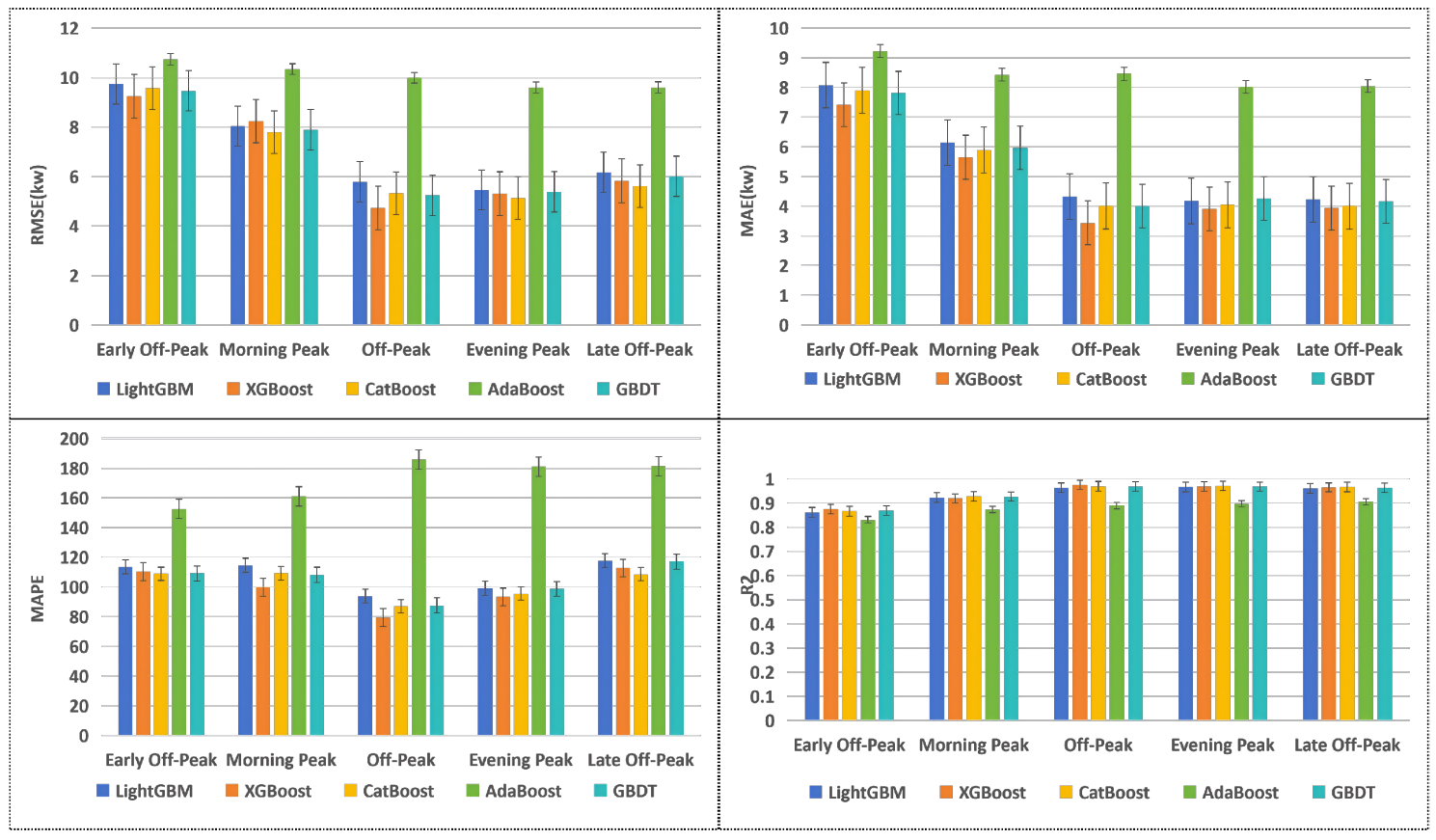
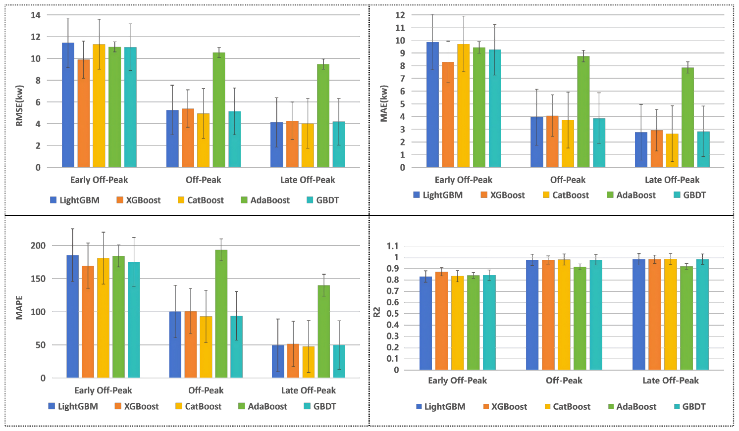
Based on actual passenger flow patterns, we define Monday to Friday as weekdays and Saturdays, Sundays, and public holidays as weekends for the analysis. Weekday traffic flow is further divided into three categories: early morning off-peak (from the start of service to 6:20 a.m.), morning peak (6:20 a.m. to 8:20 a.m.), off-peak (8:20 a.m. to 4:00 p.m.), evening peak (4:00 p.m. to 6:00 p.m.), and late evening off-peak (6:00 p.m. to the end of service). The energy consumption datasets are stratified by their collection time, and each stratified dataset is tested using the pre-constructed models. (16:00–18:00) as evening peak, and off-peak operation (8:20–16:00). Classify the feature datasets by the time at which the data was generated. Each dataset is tested using the pre-constructed models to compare the predictive performance of the different models across various traffic flow periods. The results are as follows:

Weekdays are divided into five traffic flow periods throughout the day. The five pre-constructed models are used for prediction, and one month of weekday operational data is used for the prediction tests. The results are shown in Figure 12. The results show that the XGBoost model achieves the best prediction results, though it exhibits significant prediction errors and low accuracy during the early morning off-peak period. Weekends are divided into only three traffic flow periods, with the prediction results shown in Figure 13. The results indicate that XGBoost achieves the best performance during the early morning off-peak period, while CatBoost achieves the best performance during the other two periods. The results indicate that the prediction accuracy during off-peak periods on both weekdays and weekends decreases by approximately 10% compared to other periods, and the mean squared error (MSE) is approximately twice as high as that in other periods. The variation in model prediction accuracy and error is likely related to the sample size of the stratified datasets. To validate this conclusion, we test the models’ predictive performance using datasets of different sample sizes.

5.2.2. Impact of Data Volume

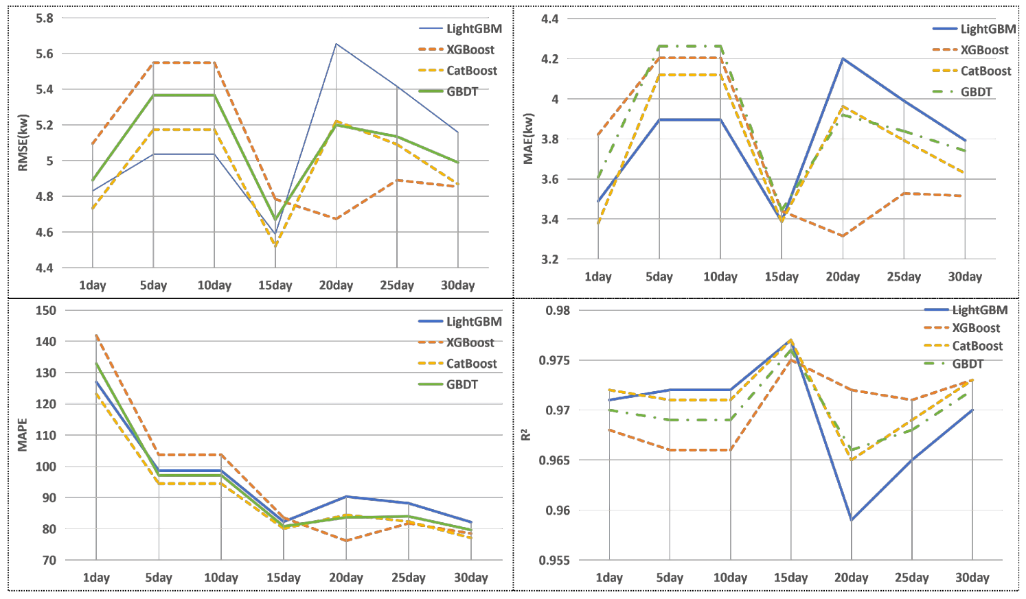
For verification purposes, operational data from the same single vehicle during 9:00 a.m. to 11:00 a.m. over 1, 5, 10, 15, 20, 25, and 30 working days are selected to construct test sets of different sample sizes. his dataset setup is used to analyze how the sample size affects the model’s predictive performance. Since the AdaBoost model performs worse than the other four algorithms during peak traffic periods, it is excluded from further comparisons. The results are shown in Figure 14. The findings reveal that all models deliver satisfactory prediction performance across all tested sample sizes, with the optimal performance achieved when using 15 days of operational data—yielding minimal prediction error and high accuracy. LightGBM exhibits better predictive performance with smaller sample sizes, while XGBoost achieves slightly better performance with larger sample sizes, though the performance difference between the two algorithms is negligible. For practical deployment, when training the models with the latest operational data to predict the vehicle’s energy consumption over a fortnight, both models deliver reliable predictive performance. For scenarios with limited sample sizes (smaller datasets), LightGBM is the preferred choice, while XGBoost is recommended for scenarios with larger sample sizes (larger datasets).

5.2.3. Impact of Vehicle Count

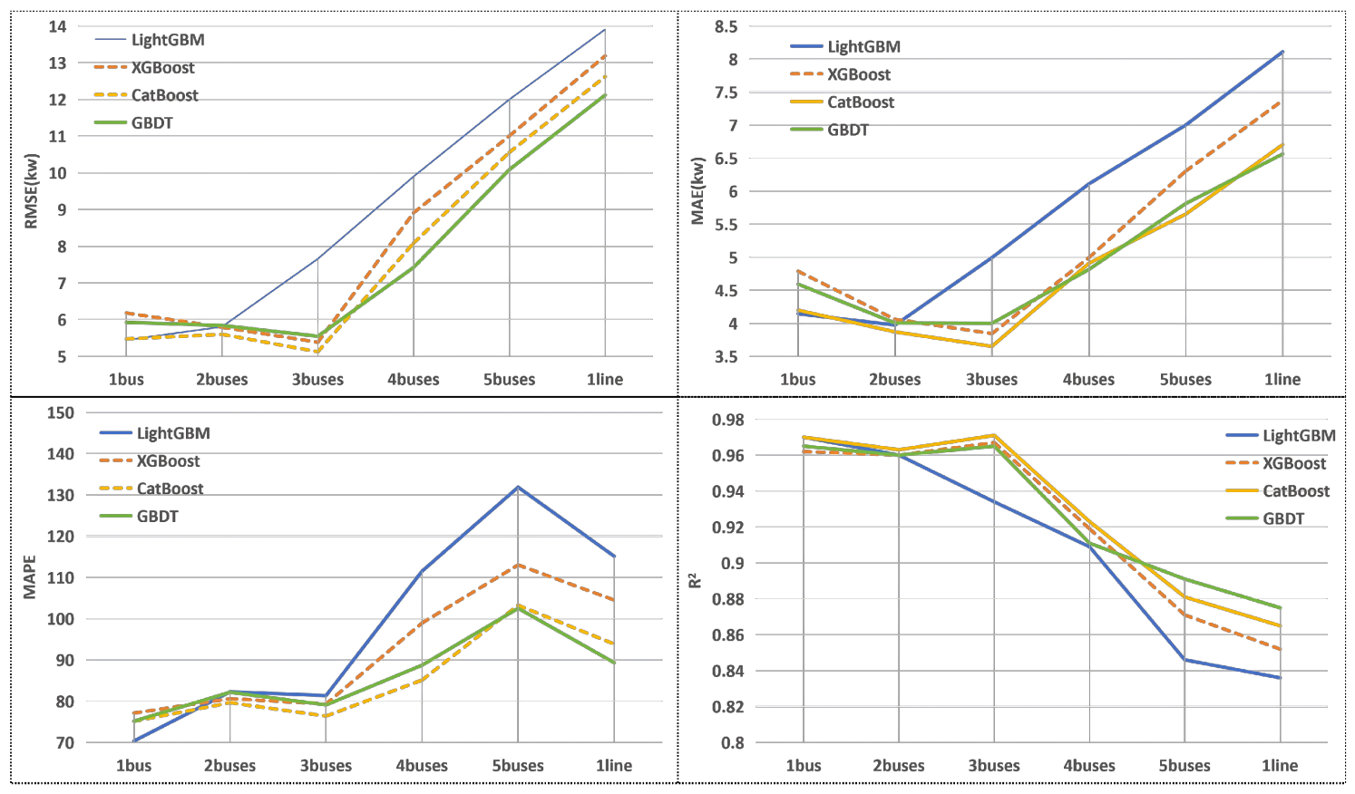
The above validation results are all based on data from a single vehicle to assess model performance. Next, we validate the model’s generalizability by using datasets constructed from different numbers of vehicles. We select all operational data from all vehicles on this route over two consecutive days and group them according to the number of vehicles included: 1, 2, 3, 4, 5 vehicles, and all vehicles on the entire route. We then test the pre-constructed models on these vehicle groups and compare the prediction results to evaluate the model’s cross-vehicle generalizability. (Since the AdaBoost model demonstrates poorer prediction performance than the other four algorithms in previous experiments, it is excluded from this comparison.) The results of the cross-vehicle validation are shown in Figure 15.

The cross-vehicle validation results show that the predictive performance of all models gradually degrades as the number of vehicles included in the dataset increases. The CatBoost model demonstrates the best performance in predicting the instantaneous energy consumption of a single vehicle. However, as the number of vehicles in the dataset increases, the prediction accuracy of the CatBoost model deteriorates, while the prediction accuracy of the GBDT model improves. Models trained on single-vehicle operational data achieve an $R^2$ of 87.5% when predicting the instantaneous energy consumption of the entire route. This represents an approximate 10% decrease in prediction accuracy compared to single-vehicle predictions, but the models still deliver robust predictive performance for route-level energy consumption prediction. However, it should be noted that these results are derived from a limited test dataset confined to a single transit route. Broader validation across different routes and vehicle types is necessary to fully establish universal applicability.

5.3. Limitations of the Study

Although the proposed framework demonstrates strong predictive performance and high interpretability, several inherent limitations regarding data representativeness and methodological assumptions warrant discussion.

The primary limitation lies in the spatiotemporal scope of the dataset, which is restricted to a single urban bus route in Jinan, China, during the winter season. Given that the energy consumption of electric buses (particularly their HVAC systems) is highly sensitive to ambient temperature and topography, the study’s findings may require further validation to ensure their generalizability across different climatic conditions and road environments. Additionally, the lack of direct passenger load data represents a significant shortcoming. Although the model incorporates certain kinematic variables that reflect fluctuations in power demand, the absence of real-time passenger load information limits the framework’s ability to explicitly account for changes in vehicle mass. Although these factors are not explicitly included, their effects are partially reflected through measurable operational variables such as speed, acceleration, torque, and temperature. Road conditions such as traffic states and road gradients are not explicitly modeled due to data availability constraints.

From a statistical perspective, the use of high-resolution, second-by-second operational data introduces potential risks associated with temporal autocorrelation. Although the algorithm itself is robust, the nature of time-series data necessitates a rigorous validation strategy to ensure that potential data leakage does not overestimate the model’s predictive performance. Furthermore, the technical scope of this study is limited to a specific bus model from a single manufacturer. Differences among manufacturers in powertrain architecture, battery chemistry, and energy management strategies may affect the cross-brand applicability of the developed model.

Regarding the physical modeling of the powertrain, the proposed model is based on simplified linear assumptions. While this modeling approach offers the advantages of high computational efficiency and ease of interpretation, it may fail to fully capture nonlinear behavior under complex operating conditions such as regenerative braking and stationary states. In particular, factors affecting energy recovery efficiency—such as state of charge (SoC), temperature-dependent charging limitations, and braking intensity—have not been explicitly modeled. Similarly, stationary conditions such as idling and auxiliary system operation may introduce additional nonlinear energy consumption characteristics. Nevertheless, the model provides a reasonable approximation of vehicle energy consumption requirements under typical driving conditions and serves as an effective baseline for data-driven optimization.

6. Conclusions

This study demonstrates how high-resolution onboard operational data combined with machine-learning methods can substantially improve the prediction of energy consumption in battery-electric bus operations. Using second-by-second data from an in-service electric bus fleet operating on Route 49 in Jinan, the paper compared a physics-based micro-level energy consumption model with data-driven approaches and evaluated their suitability for real-world public transport applications.

The physics-based model provides a transparent baseline and captures average energy consumption trends, but its predictive performance deteriorates under complex operating conditions such as regenerative braking and frequent stop-and-go service. In contrast, boosting-based machine-learning models achieve strong explanatory power and stable predictive performance, with coefficients of determination ($R^2$) of approximately 0.99 on the training set and 0.95 on the test set. These results indicate that the proposed model is effective for high-resolution power estimation and provides a reliable basis for downstream operational analysis.

Feature importance and SHAP analyses indicate that motor torque, motor speed, and vehicle speed are the dominant drivers of instantaneous energy consumption, while temperature-related variables play a secondary but stabilizing role. These results confirm that the data-driven models capture physically meaningful mechanisms and provide interpretable insights that are relevant for transit operators. The robustness analysis further shows that reliable model performance can be achieved with approximately two weeks of operational data and that models trained on individual vehicles show strong potential to be transferred to route-level applications. Nevertheless, the current findings are based on a restricted dataset from a specific fleet. Further empirical validation across diverse operational environments, seasonal variations, and larger fleets is required to comprehensively confirm the model’s superiority and generalizability.

Future research will focus on extending the proposed modeling framework to multi-seasonal datasets, diverse bus fleets, and a broader range of public transportation scenarios, thereby enhancing the model’s generalization capabilities across different climatic conditions, operational environments, and service models. The research will incorporate key operational factors such as real-time passenger load, variations in stop dwell times, and route topology, while also exploring the integration of real-time passenger load sensing technologies to optimize the model’s adaptability to actual operational scenarios; The model will be optimized to meet edge computing deployment requirements, supporting more efficient, real-time, and energy-efficient bus operation decisions. Additionally, the framework’s portability across fleets with heterogeneous vehicle types and sensor configurations, as well as across cities, will be investigated to further expand its practical application scope. Furthermore, integrating the developed energy consumption prediction model with bus schedule planning and charging infrastructure optimization, as well as combining this modeling approach with real-time fleet management systems, represent highly promising research directions. Both are expected to provide coordinated and scientifically grounded decision support for daily bus operations, thereby contributing to the development of more intelligent, data-driven, and sustainable urban transportation systems.

References

1. Dong, L.; Miao, G.; Wen, W. China’s carbon neutrality policy: Objectives, impacts and paths. East Asian Policy 2021, 13, 5–18. [Google Scholar] [CrossRef] [Scilit]
2. IEA. Global EV Outlook 2025; International Energy Agency: Paris, France, 2025. [Google Scholar]
3. Editorial. Electric Bus, Main Fleets and Projects Around the World. Sustainable Bus. Available online: https://www.sustainable-bus.com/electric-bus/electric-bus-public-transport/ (accessed on 9 October 2025).
4. Docherty, I.; Marsden, G.; Anable, J. The governance of smart mobility. Transp. Res. Part Policy Pract. 2018, 115, 114–125. [Google Scholar] [CrossRef] [Scilit]
5. Wolbertus, R.; Kroesen, M.; Van Den Hoed, R.; Chorus, C. Fully charged: An empirical study into the factors that influence connection times at EV-charging stations. Energy Policy 2018, 123, 1–7. [Google Scholar] [CrossRef] [Scilit]
6. Abdelaty, H.; Al-Obaidi, A.; Mohamed, M.; Farag, H.E.Z. Machine learning prediction models for battery-electric bus energy consumption in transit. Transp. Res. Part D Transp. Environ. 2021, 96, 102868. [Google Scholar] [CrossRef] [Scilit]
7. Chen, Y.; Zhang, Y.; Sun, R. Data-driven estimation of energy consumption for electric bus under real-world driving conditions. Transp. Res. Part D Transp. Environ. 2021, 98, 102969. [Google Scholar] [CrossRef] [Scilit]
8. Genikomsakis, K.N.; Mitrentsis, G. A computationally efficient simulation model for estimating energy consumption of electric vehicles in the context of route planning applications. Transp. Res. Part D Transp. Environ. 2017, 50, 98–118. [Google Scholar] [CrossRef] [Scilit]
9. Luin, B.; Petelin, S.; Al-Mansour, F. Microsimulation of electric vehicle energy consumption. Energy 2019, 174, 24–32. [Google Scholar] [CrossRef] [Scilit]
10. Wang, J.; Elbery, A.; Rakha, H.A. A real-time vehicle-specific eco-routing model for on-board navigation applications capturing transient vehicle behavior. Transp. Res. Part C Emerg. Technol. 2019, 104, 1–21. [Google Scholar] [CrossRef] [Scilit]
11. Ye, F.; Wu, G.; Boriboonsomsin, K.; Barth, M.J. A hybrid approach to estimating electric vehicle energy consumption for ecodriving applications. In Proceedings of the 2016 IEEE 19th International Conference on Intelligent Transportation Systems (ITSC), Rio de Janeiro, Brazil, 1–4 November 2016; pp. 719–724. [Google Scholar]
12. Chen, Y.; Wu, G.; Sun, R.; Dubey, A.; Laszka, A.; Pugliese, P. A review and outlook on energy consumption estimation models for electric vehicles. SAE Int. J. Sustain. Transp. Energy Environ. Policy 2021, 2, 79–96. [Google Scholar] [CrossRef] [Scilit]
13. Li, W.; Stanula, P.; Egede, P.; Kara, S.; Herrmann, C. Determining the Main Factors Influencing the Energy Consumption of Electric Vehicles in the Usage Phase. Procedia CIRP 2016, 48, 352–357. [Google Scholar] [CrossRef] [Scilit]
14. Donkers, A.; Yang, D.; Viktorović, M. Influence of driving style, infrastructure, weather and traffic on electric vehicle performance. Transp. Res. Part D Transp. Environ. 2020, 88, 102569. [Google Scholar] [CrossRef] [Scilit]
15. Liu, K.; Wang, J.; Yamamoto, T.; Morikawa, T. Exploring the interactive effects of ambient temperature and vehicle auxiliary loads on electric vehicle energy consumption. Appl. Energy 2018, 227, 324–331. [Google Scholar] [CrossRef] [Scilit]
16. Al-Wreikat, Y.; Serrano, C.; Sodré, J.R. Effects of ambient temperature and trip characteristics on the energy consumption of an electric vehicle. Energy 2022, 238, 122028. [Google Scholar] [CrossRef] [Scilit]
17. Min, H.; Zhang, Z.; Sun, W.; Min, Z.; Yu, Y.; Wang, B. A thermal management system control strategy for electric vehicles under low-temperature driving conditions considering battery lifetime. Appl. Therm. Eng. 2020, 181, 115944. [Google Scholar] [CrossRef] [Scilit]
18. Al-Wreikat, Y.; Serrano, C.; Sodré, J.R. Driving behaviour and trip condition effects on the energy consumption of an electric vehicle under real-world driving. Appl. Energy 2021, 297, 117096. [Google Scholar] [CrossRef] [Scilit]
19. Bracco, S.; Bianco, G.; Siri, S.; Barbagelata, C.; Casati, C.; Siri, E. Simulation models for the evaluation of energy consumptions of electric buses in different urban traffic scenarios. In Proceedings of the 2021 Sixteenth International Conference on Ecological Vehicles and Renewable Energies (EVER), Monte-Carlo, Monaco, 5–7 May 2021; pp. 1–6. [Google Scholar]
20. Di Martino, A.; Miraftabzadeh, S.M.; Longo, M. Strategies for the modelisation of electric vehicle energy consumption: A review. Energies 2022, 15, 8115. [Google Scholar] [CrossRef] [Scilit]
21. Miri, I.; Fotouhi, A.; Ewin, N. Electric vehicle energy consumption modelling and estimation—a case study. Int. J. Energy Res. 2021, 45, 501–520. [Google Scholar] [CrossRef] [Scilit]
22. Hjelkrem, O.A.; Lervåg, K.Y.; Babri, S.; Lu, C.; Södersten, C.-J. A battery electric bus energy consumption model for strategic purposes: Validation of a proposed model structure with data from bus fleets in China and Norway. Transp. Res. Part D Transp. Environ. 2021, 94, 102804. [Google Scholar] [CrossRef] [Scilit]
23. Fiori, C.; Ahn, K.; Rakha, H.A. Power-based electric vehicle energy consumption model: Model development and validation. Appl. Energy 2016, 168, 257–268. [Google Scholar] [CrossRef] [Scilit]
24. Abdelaty, H.; Mohamed, M. A framework for BEB energy prediction using low-resolution open-source data-driven model. Transp. Res. Part D Transp. Environ. 2022, 103, 103170. [Google Scholar] [CrossRef] [Scilit]
25. Lin, X.; Zhang, G.; Wei, S.; Yin, Y. Energy consumption estimation model for dual-motor electric vehicles based on multiple linear regression. Int. J. Green Energy 2020, 17, 488–500. [Google Scholar] [CrossRef] [Scilit]
26. Pokharel, S.; Sah, P.; Ganta, D. Improved prediction of total energy consumption and feature analysis in electric vehicles using machine learning and shapley additive explanations method. World Electr. Veh. J. 2021, 12, 94. [Google Scholar] [CrossRef] [Scilit]
27. Liu, X.; Zhao, F.; Geng, J.; Hao, H.; Liu, Z. Comprehensive assessment for different ranges of battery electric vehicles: Is it necessary to develop an ultra-long range battery electric vehicle? iScience 2023, 26, 106654. [Google Scholar] [CrossRef] [Scilit]
28. Ullah, I.; Liu, K.; Yamamoto, T.; Zahid, M.; Jamal, A. Electric vehicle energy consumption prediction using stacked generalization: An ensemble learning approach. Int. J. Green Energy 2021, 18, 896–909. [Google Scholar] [CrossRef] [Scilit]
29. Pan, Y.; Fang, W.; Zhang, W. Development of an energy consumption prediction model for battery electric vehicles in real-world driving: A combined approach of short-trip segment division and deep learning. J. Clean. Prod. 2023, 400, 136742. [Google Scholar] [CrossRef] [Scilit]
30. Li, S.; Zhang, H.; Tan, H.; Zhong, Z.; Jiang, Z. An Attention-Based Model for Travel Energy Consumption of Electric Vehicle with Traffic Information. Adv. Civ. Eng. 2021, 2021, 5571271. [Google Scholar] [CrossRef] [Scilit]
31. Xing, Y.; Li, Y.; Liu, W.; Li, W.; Meng, L. Operation Energy Consumption Estimation Method of Electric Bus Based on CNN Time Series Prediction. Math. Probl. Eng. 2022, 2022, 6904387. [Google Scholar] [CrossRef] [Scilit]
32. Lundberg, S.M.; Lee, S.-I. A Unified Approach to Interpreting Model Predictions. arXiv 2017, arXiv:1705.07874v2. [Google Scholar] [CrossRef] [Scilit]
33. Lundberg, S.M.; Erion, G.G.; Lee, S.-I. Consistent Individualized Feature Attribution for Tree Ensembles. arXiv 2019, arXiv:1802.03888. [Google Scholar] [CrossRef] [Scilit]
34. Guo, J.; Jiang, Y.; Yu, Y.; Liu, W. A novel energy consumption prediction model with combination of road information and driving style of BEVs. Sustain. Energy Technol. Assess. 2020, 42, 100826. [Google Scholar] [CrossRef] [Scilit]
35. Lajunen, A.; Kivekaes, K.; Baldi, F.; Vepsaelaeinen, J.; Tammi, K. Different approaches to improve energy consumption of battery electric buses. In Proceedings of the 2018 IEEE Vehicle Power and Propulsion Conference (VPPC), Chicago, IL, USA, 27–30 August 2018; pp. 1–6. [Google Scholar]
Figure 1. Research framework diagram.
Energies 19 02058 g001
Figure 2. The studied bus route 49.
Energies 19 02058 g002
Figure 3. 30 M High-resolution digital elevation model map.
Energies 19 02058 g003
Figure 4. Bus operation status classifications.
Energies 19 02058 g004
Figure 5. Forces acting on a bus during operation.
Energies 19 02058 g005
Figure 6. RMSE Optimization Trend for All Models.
Energies 19 02058 g006
Figure 7. Scatter plot comparing predicted values and actual values.
Energies 19 02058 g007
Figure 8. Trends of prediction values across algorithms.
Energies 19 02058 g008
Figure 9. Analysis of Model Prediction Errors and Stability.
Energies 19 02058 g009
Figure 10. SHAP-based interpretability analysis of the XGBoost model. (ah) SHAP dependence plots showing the relationship between feature values and their contributions to the predicted power, including CAN speed, acceleration, motor torque, motor speed, interior temperature, and exterior temperature. The color scale represents the interaction effect with secondary features. Red curves indicate the overall trend of feature influence.
Energies 19 02058 g010
Figure 11. SHAP Analysis of feature impact on the model.
Energies 19 02058 g011
Figure 12. Comparison of traffic flow forecasts by model for weekday time periods.
Energies 19 02058 g012
Figure 13. Comparison of traffic flow forecasts by model for weekend Time periods.
Energies 19 02058 g013
Figure 14. Impact of dataset size on model prediction.
Energies 19 02058 g014
Figure 15. Impact of different vehicle datasets on models.
Energies 19 02058 g015