Coordinated Defense Strategies for Energy Storage Systems Against Cascading Faults in Extreme Grid Scenarios

Abstract

To address the vulnerability of renewable-dominated power grids to cascading failures under extreme conditions and the limitations of existing methods in jointly handling vulnerability identification, energy storage allocation, and online control, this paper proposes an energy-storage-assisted coordinated defense strategy. First, a source-load uncertainty model is constructed and seven typical extreme operating scenarios are identified. Second, a cascading-failure evolution model that accounts for thermal accumulation is established to identify critical vulnerable branches. Third, for areas prone to local disconnection and weak terminal voltages, a coordinated ESS allocation model is developed by jointly considering active power, energy capacity, and reactive power support to determine candidate deployment locations and capacities. Finally, a graph neural network (GNN) is used to extract time-varying topological and electrical-state features, and proximal policy optimization (PPO) is employed to generate coordinated control commands for multiple ESSs, thereby linking overload suppression with voltage support. The results for the modified IEEE 39-bus system show that the proposed method identifies high-risk branches more accurately and forms an integrated defense chain covering identification, allocation, and control. The method reduces thermal stress in critical sections during the early stage of a fault, mitigates load shedding, and enhances system survivability.

1. Introduction

In recent years, the combination of high proportions of renewable energy being fed into the grid, a decline in system inertia and frequent extreme weather events has led to a continuous narrowing of the safety margins for power system operations. Local disturbances are now more likely to escalate into widespread blackouts under the combined effects of power flow shifts, protection system operations and deteriorating operational conditions. The 2023 Pakistan blackout, the 2021 Texas cold snap blackout, the 2021 European grid separation, and the 2019 United Kingdom power outage demonstrate that modern power grids exhibit greater vulnerability under complex disturbances [1,2,3,4]. Existing accident analyses and review studies have indicated that when the system is under heavy load, weak support, or extreme external forcing conditions, initial faults are more likely to propagate along critical sections and trigger cascading consequences [5,6]. Consequently, research into the mechanisms of cascading fault propagation under extreme scenarios, the identification of critical vulnerabilities, and proactive defense methods has become a key issue in the safe operation of new-generation power systems.

Existing research on the mechanisms of cascading fault propagation and vulnerability identification can be broadly categorized into three types. The first category of methods is based on complex network theory and utilizes metrics such as node centrality, line degree and network connectivity to identify system vulnerabilities [7,8]. These methods are computationally efficient and suitable for the rapid screening of large-scale systems; however, they do not adequately account for operational states or the temporal progression of fault propagation. The second category of methods takes an electrical perspective, employing cascade failure models, N-k safety analysis and fault scenario simulation to characterize the evolution of faults under power flow redistribution [9,10,11,12]. Compared with topological analysis, these methods better capture fault propagation paths and the influence of critical components; however, many models still rely on static out-of-limit criteria and do not sufficiently account for thermal accumulation in lines or the sequential approach of faults under extreme conditions. Overall, existing research has laid the groundwork for the identification of cascading faults, but there remains a lack of analytical frameworks capable of simultaneously reflecting extreme operating scenarios, thermal accumulation effects, and the dynamic migration characteristics of critical vulnerable branches.

Existing research on the role of energy storage in enhancing grid resilience and the allocation of defense resources has largely focused on two aspects. One category of studies aims to optimize economic operation and the integration of renewable energy, analyzing the role of energy storage in peak shaving and valley filling, improving the utilization rate of renewable energy, and reducing operational costs [13,14]. The other category of research discusses energy storage deployment from the perspectives of disturbance resilience and system security, highlighting that energy storage can utilize its rapid response capabilities to enhance short-term system security and play a role in supporting vulnerable areas [15,16,17,18]. These studies demonstrate that energy storage is no longer merely a conventional regulating resource, but is increasingly being utilized to enhance system resilience. However, most existing methods focus on single functions, with greater attention paid to active power compensation, frequency support or conventional configuration optimization. Consideration of scenarios where local disconnection, power imbalance and insufficient reactive power support coexist under cascading fault conditions remains inadequate, and there is a relative lack of regionalized configuration approaches that account for the evolution of faults.

Beyond the above resilience-oriented planning and support studies, recent research has also emphasized converter-level coordination and distributed control in hybrid AC/DC architectures. For instance, regarding distributed secondary control and communication-aware coordination, Espina et al. [19] and Yang et al. [20] developed consensus-based frameworks to achieve voltage/frequency restoration while reducing communication burdens. In parallel, from the perspective of coordination-based power management, Salman et al. [21] and Mahmoudian et al. [22] proposed adaptive strategies centered on interlinking converters, enabling coordinated active/reactive power sharing across AC and DC subgrids under stressed operating conditions. Although these studies are mainly oriented to hybrid AC/DC microgrids and converter-level coordination, they provide useful insights into distributed power sharing, coordinated voltage/frequency regulation, and communication-aware control design. Nevertheless, they do not directly address the coupled problem of dynamic vulnerability identification, ESS allocation, and coordinated online defense against cascading failures in transmission grids. Motivated by these ideas, the present study further investigates the coordinated control of spatially distributed ESSs at the transmission-grid level for cascading-failure defense.

Furthermore, existing studies on energy storage systems for grid resilience predominantly focus on pre-event static capacity planning or post-event passive restoration [23,24]. While these methods effectively allocate emergency backup resources, they inherently decouple static capacity planning from millisecond-level online topological dynamic control [25,26]. Consequently, ESSs are often treated as passive power sources rather than dynamic, topology-aware regulating units, restricting their capability to suppress the rapid propagation of cascading failures. To bridge this structural gap, there is an urgent need to establish an integrated closed-loop defense framework that links offline vulnerability screening and static resource planning tightly with online dynamic defense.

In recent years, deep reinforcement learning has shown great promise for application in the emergency control of power systems, particularly in the context of artificial intelligence and collaborative defense control [27,28]. Relevant research indicates that reinforcement learning methods can enhance online decision-making efficiency through interaction with the environment and possess strong adaptability in high-dimensional non-linear scenarios. However, from the perspective of defense against cascading faults, existing methods still have shortcomings: on the one hand, traditional reinforcement learning typically simplifies the system state into vector inputs, offering limited expression of graph-structural features such as topological reconstruction, island formation and risk migration; on the other hand, existing graph learning research largely remains at the perception and evaluation stage, failing to form a tight closed-loop with continuous control. Particularly during the evolution of cascading faults, system risks continuously change with line disconnection, power flow migration and local disconnection; defense control requires dynamic adjustment as the process progresses, and such multi-stage collaborative characteristics remain inadequately addressed in current research. Specifically, many existing DRL-based emergency control approaches primarily focus on discrete actions such as load shedding, generator redispatch, or topology adjustment, while the role of multiple spatially distributed ESSs is either absent or treated only as an auxiliary control variable without reactive power considerations [29,30]. Traditional vector-based DRL models struggle to capture the spatial topological mutations during cascading propagation. Although some studies have explored topology-aware models for generation redispatch [31], the implementation of multi-ESS coordinated active and reactive dynamic support under varying topologies remains largely unexplored.

In summary, substantial progress has been made in cascading-failure identification, ESS planning, and intelligent control. However, these three aspects remain insufficiently integrated. Existing fault-identification studies pay limited attention to the continuous evolution of thermal accumulation under extreme scenarios. ESS planning still lacks a three-dimensional coordinated configuration approach for local autonomy and fault defense. Intelligent control has not yet fully adapted to rapid topological changes and multi-stage risk migration. To address these gaps, this paper investigates coordinated defense against cascading failures in power grids under extreme scenarios, as outlined below:

• A thermal-accumulation-aware vulnerability identification framework is developed for extreme operating scenarios, enabling the tracking of critical-branch migration during fault evolution.
• A three-dimensional coordinated ESS allocation model is established by jointly considering active power, energy capacity, and reactive power support, so as to support zoned siting and coordinated sizing in vulnerable areas.
• A graph-structured multi-ESS coordinated defense framework is proposed, in which GNN encodes topology-varying system states and PPO generates coordinated active/reactive control actions, thereby linking offline identification and allocation with online dynamic defense.

2. The Evolutionary Mechanisms of Cascading Failures in Extreme Scenarios and the Need for Coordinated Defense

2.1. Temporal Evolution Mechanism of Cascading Failures

A cascading failure in a power grid is not a widespread blackout caused directly by the failure of a single component, but rather a dynamic process that gradually escalates following the triggering of an initial disturbance through a sequence of power flow redistribution, local stress accumulation, protection operation and network reconfiguration. In grids with a high proportion of renewable energy, this process often exhibits greater uncertainty. On the one hand, fluctuations in generation and load, as well as power flow reversals, can cause certain critical sections to operate under high stress for extended periods; on the other hand, extreme weather conditions can alter the external thermal boundary of power lines and increase the risk of equipment failure, making it more likely for local disturbances to occur at the system’s weakest points. Following an initial fault, power is redistributed along adjacent pathways; while some lines may not trip immediately, their conductor temperatures continue to rise, and thermal safety margins are progressively eroded, causing the system to enter a sensitive phase prior to fault propagation. If the power flow at critical sections cannot be promptly suppressed and local voltage levels maintained during this phase, subsequent events such as the successive withdrawal of lines, local disconnection, and worsening power imbalance may occur, ultimately evolving into a large-scale power outage. Therefore, between the occurrence of a fault and the system entering irreversible expansion, there is in fact an intervention window dominated by thermal accumulation. Accurately identifying high-risk branches and rapidly mobilizing defense resources within this window is key to preventing cascading faults under extreme scenarios.

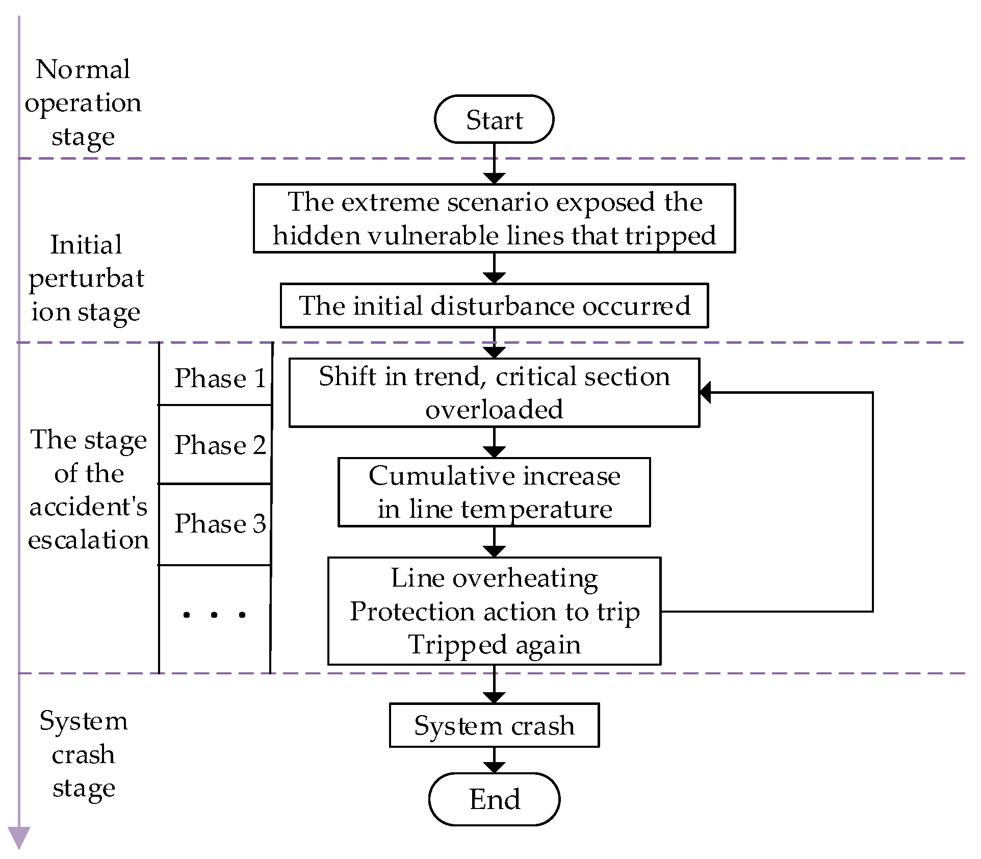
This paper focuses on the initial stage of a typical fault sequence, namely the continuous propagation process following an initial disturbance, which is driven by the interaction among power-flow changes, thermal-stress accumulation, and protection actions. It characterizes the risk-propagation pathways that can be mitigated through early ESS intervention. The temporal logic of this process is illustrated in Figure 1.

During normal operation, the system remains balanced, but under extreme conditions it often operates close to its security limits. The initial disturbance phase is typically triggered by external disturbances or equipment failures and lasts for only a short time. The subsequent accident-propagation phase is the critical stage in fault spread. Because components such as transmission lines and transformers exhibit thermal inertia, a period of thermal accumulation exists between the onset of overload and the actual operation of protection devices. This period may last for several minutes and represents the transition from a local fault to a system-wide collapse. If the fault is not effectively contained during this interval, the system may enter the collapse phase, leading to voltage or frequency instability and widespread outages.

2.2. Mechanisms of Fault Initiation and Propagation Under Extreme Conditions

The impact of extreme scenarios on cascading-failure propagation is reflected not only in the probability of an initial failure but also in simultaneous changes in the system operating state and in the pathways along which failures propagate.

In scenarios such as maximum net load and maximum gradient, the backbone sections are subjected to prolonged heavy loads, significantly reducing the regulation margin of conventional units; should any local lines be taken out of service, power flows are more likely to concentrate on adjacent routes. In scenarios such as maximum renewable energy output and worst-case voltage conditions, changes in power flow direction, insufficient local reactive power support and the vulnerability of receiving-end voltages combine to further exacerbate the consequences of a fault.

Unlike traditional static out-of-limit criteria, the risk associated with line overloading is not resolved instantaneously; there is a continuous evolutionary process between the rise in conductor temperature and the activation of protection. This process constitutes a critical transitional phase in which a cascading fault progresses from a local disturbance to topological disconnection. During this phase, the local response of a single device often struggles to simultaneously address peak shaving at the fault section, regional power support and voltage maintenance at vulnerable nodes. Energy storage, however, possesses rapid active power regulation and local reactive power support capabilities, enabling it to alter the subsequent power flow distribution and the direction of risk evolution during the early stages of fault propagation. When multiple ESS units act in coordination according to network topology and real-time operating status, they can cover multiple critical areas spatially, provide both overload suppression and voltage support functionally, and intervene continuously from the early stage of a fault through its propagation. Therefore, preventing cascading failures under extreme scenarios is not a single-point control problem but a coordinated defense problem centered on critical sections, vulnerable areas, and dynamic evolution.

Based on the above analysis, this paper breaks down the problem of preventing and controlling cascading faults under extreme scenarios into three interrelated stages: firstly, identifying key vulnerable branches that undergo dynamic migration under the influence of source-load fluctuations in extreme conditions; secondly, completing the zonal allocation and capacity matching of energy storage resources to meet the requirements for local disconnection and support of vulnerable areas; and thirdly, organizing coordinated control of multiple energy storage systems in response to topological changes and risk states during the evolution of faults. Focusing on these three stages, the subsequent sections will explore dynamic vulnerability identification, three-dimensional energy storage configuration, and online coordinated defense, respectively.

3. A Model for Identifying Dynamic Vulnerabilities in Power Grids Under Extreme Conditions

3.1. Identification of Extreme Scenarios

3.1.1. Source-Load Uncertainty Modeling

In power grids with a high proportion of renewable energy, the system’s operating state is influenced by fluctuations in wind power, solar power and load. To identify the operating conditions most detrimental to system safety, this paper constructs baseline models for wind power, solar power and load based on historical time-series data, and introduces random disturbances to account for short-term forecasting errors. On this basis, a set of source-load samples required for extreme scenario analysis is generated.

• Wind power output model

To account for the uncertainty in the forecasts, the historical wind power data was normalized to produce a trend curve for wind power generation $Tren{d}_{wind}(t)$, as shown in Equation (1):

$$Tren{d}_{wind}(t)={\displaystyle \frac{P_{wind}^{measured}(t)}{\max (P_{wind}^{measured})}}$$

(1)

where $P_{wind}^{measured}(t)$ represents the historical measured wind power output at time $t$.

For wind turbines connected to the grid busbar, the calculation of their actual output $P_{wind,i}(t)$ at any given time is shown in Equation (2):

$$P_{wind,i}(t)=Tren{d}_{wind}(t)\cdot P_{max,i}^{gen}\cdot (1+{\delta }_{wind})$$

(2)

where $P_{max,i}^{gen}$ is the rated capacity of the wind turbine; ${\delta }_{wind}$ is a random noise term following a normal distribution, simulating fluctuations in local wind speed.

2.

Photovoltaic power output model

Photovoltaic power output is significantly affected by solar irradiance and cloud cover. This paper employs a clear-sky model combined with random noise for modeling. First, the theoretical clear-sky irradiance coefficient $G_{clear}(t)$ is calculated based on the time of day $t_{hour}$, as shown in Equation (3):

$$G_{clear}(t)=\max \left(0,\sin \left(\pi \cdot {\displaystyle \frac{t_{hour}-t_{rise}}{t_{set}-t_{rise}}}\right)\right)$$

(3)

where $t_{rise}$, $t_{set}$ are the times of sunrise and sunset.

The raw output $P_{pv,j}^{raw}(t)$ of the photovoltaic power station connected to busbar $j$ is calculated using Equation (4), while the smoothed output $P_{pv,j}(t)$ is calculated using Equation (5):

$$P_{pv,j}^{raw}(t)=P_{max,j}^{gen}\cdot G_{clear}(t)\cdot {\xi }_{pv}(t)$$

(4)

$$P_{pv,j}(t)=\mathrm{Smooth}(P_{pv,j}^{raw}(t),w)$$

(5)

where ${\xi }_{pv}(t)$ is the photovoltaic noise factor; window size $w=12$.

3.

Dynamic load model

The load curve is modeled using a typical bimodal characteristic. The actual active load $P_{load,k}(t)$ at node $k$ in the power grid at time $t$ is given by Equation (7), where the normalized load factor is calculated as shown in Equation (6):

$$\begin{array}{r}{\rho }_{load}(t)=C_{base}-\alpha \cdot \tanh (\beta \cdot (t_{hour}-t_{morning}))\\ +\alpha \cdot \tanh (\beta \cdot (t_{hour}-t_{evening}))+{ϵ}_{load}\end{array}$$

(6)

$$P_{load,k}(t)=P_{base,k}\cdot {\rho }_{load}(t)$$

(7)

where $P_{base,k}$ represents the base load of the busbar; $\alpha$ and $\beta$ represent the amplitude and steepness of load variation; $t_{morning}$ and $t_{evening}$ represent the times at which the morning load rises and the evening load falls; ${ϵ}_{load}$ represents the random disturbance term.

Based on the generation and load data defined above, the concept of net load is introduced. Net load directly reflects the regulation pressure borne by conventional generating units and serves as a key indicator of system flexibility. The net load $P_{net}(t)$ of the system at time $t$ is defined as shown in Equation (8):

$$P_{net}(t)={\displaystyle \sum _{k\in L}{P}_{load,k}}(t)-\left({\displaystyle \sum _{i\in W}{P}_{wind,i}}(t)+{\displaystyle \sum _{j\in V}{P}_{pv,j}}(t)\right)$$

(8)

In the equation, $L$, $W$ and $V$ represent the load set, wind power set and solar power set, respectively.

Although the source-load uncertainty model in this study captures the baseline variability in renewable generation and load through historical profiles with stochastic perturbations, it does not explicitly model the spatial correlation among geographically distributed plants, the temporal autocorrelation of outputs, or the clustering characteristics of extreme weather events. In a more generalized theoretical setting, these complex spatiotemporal dynamics can be mathematically represented by joint stochastic-process models—such as copula-based spatial dependence models, autoregressive moving average (ARMA) and vector autoregressive moving average (VARMA) temporal models, and cluster-aware extreme-event representations. However, such formulations were not explicitly implemented in the present study and are discussed here to clarify the broader modeling scope. Since the main objective of this paper is to verify the efficacy of the coordinated defense control framework rather than to construct a full meteorological scenario generator, a simplified scenario extraction method is adopted. This treatment intends to provide representative boundary conditions for evaluating the proposed control strategy, while the fully coupled joint stochastic evolution of meteorological extremes is left for future work.

3.1.2. Identification of Extreme Scenarios in Renewable-Dominated Power Grids with High Penetration

• Extreme scenarios for supply–demand balance

The maximum net load scenario $t_{s1}$ corresponds to the moment when the system supply pressure is at its highest, as shown in Equation (9). At this point, the net supply burden on conventional units is at its heaviest, the system operating margin is relatively low, and critical sections are more prone to overload and power imbalance following disturbances; this is therefore a key scenario for assessing the risk of cascading failures under extreme overload conditions:

$$t_{s1}=\arg \underset{t}{\max }{P}_{net}(t)$$

(9)

The minimum net load scenario $t_{s2}$ corresponds to the point in time when the system’s peak-shaving pressure is at its highest, as shown in Equation (10). At this point, the pressure to integrate renewable energy is particularly acute, and local areas are prone to issues such as high voltage and power flow reversal; this scenario can be used to characterize the operational limits of the system under conditions of high renewable energy penetration.

$$t_{s2}=\arg \underset{t}{\min }{P}_{net}(t)$$

(10)

2.

Extreme Renewable-Generation Scenarios

Scenario $t_{s3}$, representing the maximum total output from renewable energy sources, corresponds to the moment when the system receives the highest injection of renewable energy, as shown in Equation (11). At this point, a large amount of electrical energy is transmitted from the renewable energy aggregation area to the load center, causing a significant increase in power flow pressure on the transmission lines, which makes it easier to identify the risk of overload at critical sections:

$$t_{s3}=\arg \underset{t}{\max }\left({\displaystyle \sum _{i\in W}{P}_{wind,i}}(t)+{\displaystyle \sum _{j\in V}{P}_{pv,j}}(t)\right)$$

(11)

The maximum wind power output scenario $t_{s4}$ is shown in Equation (12):

$$t_{s4}=\arg \underset{t}{\max }{\displaystyle \sum _{i\in W}{P}_{wind,i}}(t)$$

(12)

The maximum photovoltaic power output scenario $t_{s5}$ is shown in Equation (13):

$$t_{s5}=\arg \underset{t}{\max }{\displaystyle \sum _{j\in V}{P}_{pv,j}}(t)$$

(13)

As wind and solar resources are spatially and temporally complementary but also exhibit asynchronous characteristics, analyzing the output of these two types of renewable energy separately helps to identify localized issues that might otherwise be masked by the aggregate output and to pinpoint local grid vulnerabilities at specific resource connection points.

3.

Dynamic security boundary condition scenarios

The maximum ramping rate scenario $t_{s6}$ corresponds to the moment when the system’s net load changes most rapidly, as shown in Equation (14). This scenario reflects the operating conditions under which the system’s flexibility resources are under the greatest strain, and can be used to assess regulation risks under conditions of rapid source-load changes.

$$t_{s6}=\arg \underset{t}{\max }\left|{\displaystyle \frac{P_{net}(t)-P_{net}(t-\Delta t)}{\Delta t}}\right|$$

(14)

The worst-case voltage scenario $t_{s7}$ corresponds to the moment when the system’s overall voltage deviates most significantly from the reference value, as shown in Equation (15). This scenario reflects an operational state characterized by insufficient reactive power support and significant voltage risks in weak areas of the load center, and can be used to identify the critical moments when voltage safety margins are at their tightest.

$$t_{s7}=\arg \underset{t}{\max }\left({\displaystyle \sum _{i\in N}|}{V}_i(t)-V_{ref}|\right)$$

(15)

3.2. A Cascading-Failure Evolution Model Accounting for Thermal Accumulation Effects

3.2.1. Dynamic Thermal Equilibrium Model for Transmission Conductors

During cascading failures, power flow redistribution may cause severe overloading on in-service transmission branches. The resulting thermal accumulation may further trigger subsequent tripping, thereby aggravating network disconnection and accelerating fault propagation. To capture this transient thermal behavior more accurately, this study adopts a dynamic thermal equilibrium model formulated according to IEEE Std 738, in which the conductor temperature evolution is governed by Joule heating, solar heat gain, convective cooling, and radiative cooling. The overall dynamic heat balance equation per unit length is expressed as

$$C_p\cdot m\cdot {\displaystyle \frac{d{T}_l}{dt}}=q_I+q_s-q_c-q_r$$

(16)

where $T_l$ is the temperature of line $l$. The respective heat terms are defined as follows:

$$q_I=I^{2}R(T_l)$$

(17)

$$q_s={\alpha }_s{S}_{sun}D$$

(18)

$$q_c=\max (q_{c,nat},q_{c,force})$$

(19)

$$q_r=\pi D\epsilon {\sigma }_B[{(T_l+273.15)}^4-{(T_a+273.15)}^4]$$

(20)

where $C_p$ is the specific heat capacity of the conductor material; $T_l$ is the temperature of line $l$; $m$ is the mass of the conductor per unit length; $q_I$, $q_s$, $q_c$ and $q_r$ represent, in order, the current, heat gain from solar radiation, convective heat loss and radiative heat loss. $R(T_l)$ is the temperature-dependent AC resistance of the conductor, updated dynamically via $R(T_l)=R_{ref}[1+{\alpha }_T(T_l-T_{ref})]$. The convective cooling term $q_c$ takes the maximum value between natural convection $q_{c,nat}$ and forced convection $q_{c,force}$, where $q_{c,force}$ is dynamically corrected by the wind attack angle ${\delta }_{wind}$. For implementation in the discrete-time cascading-failure simulation framework, the above nonlinear differential equation is discretized using the forward Euler method, yielding the conductor-temperature update equation at each simulation step:

$$T_l(t+\Delta t)=T_l(t)+{\displaystyle \frac{\Delta t}{C_p\cdot m}}\left[q_I(t)+q_s(t)-q_c(t)-q_r(t)\right]$$

(21)

where $\Delta t$ is the simulation step size.

To improve methodological transparency and reproducibility, the key physical parameters, environmental settings, and air-property parameters used in the dynamic thermal simulation are explicitly listed in

Table 1. Key parameters of the dynamic thermal equilibrium model based on IEEE Std 738.

Category	Symbol	Description	Value	Unit
Conductor physical/material parameters	$D$	Conductor diameter	0.02812	m
	$m$	Conductor mass per unit length	1.628	kg/m
	Cp	Specific heat capacity	700	J/(kg·°C)
	${\alpha }_T$	Temperature coefficient of resistance	0.004308	1/°C
	$R_{ref}$	Reference resistance per unit length	0.23 × 10−4	Ω/m
	$T_{ref}$	Reference temperature for resistance correction	40	°C
	${\alpha }_s$	Solar absorptivity	0.5	-
	$\epsilon$	Emissivity	0.5	-
Environmental and operating settings for case study	Ta	Ambient temperature	35	°C
	$S_{sun}$	Solar radiation intensity	1000	W/m2
	$v_w$	Wind speed	0.61	m/s
	${\delta }_{wind}$	Wind attack angle	45	°
	${\sigma }_B$	Stefan–Boltzmann constant	5.67 × 10−8	W/(m2·K4)
Air-property parameters used in convection calculation	${\rho }_f$	Air density	1.127	kg/m3
	${\lambda }_f$	Air thermal conductivity	0.02662	W/(m·K)
	${\mu }_f$	Air dynamic viscosity	1.918 × 10−5	Pa·s

.

3.2.2. Protection Action Criteria and Fault Expansion Mechanism

Based on the aforementioned dynamic thermal equilibrium model, this paper further defines the operating criteria for line overload protection. When the line temperature exceeds the set maximum permissible short-term temperature and remains above this threshold for a specified duration, the protective device operates and disconnects the line. It should be noted that the purpose of adopting a thermal accumulation criterion in this paper is to approximate the risk progression process from sustained overload to protection operation, rather than to simulate the natural melting of conductors. Compared with instantaneous tripping methods based on static limit violations, this model is capable of describing the process by which the thermal safety margin of a line diminishes over time, thereby providing a physical foundation that better aligns with the laws of fault evolution for subsequent analyses of cascading fault propagation and coordinated defense control.

3.3. A Comprehensive Method for Identifying Vulnerable Branches

To identify critical paths that significantly impact system operational safety under extreme scenarios, this paper constructs a fault sample set based on seven typical extreme scenarios and conducts batch-based cascading fault simulations. On this basis, the vulnerability of lines is comprehensively characterized from two dimensions: fault occurrence frequency and severity of consequences. Specifically, fault frequency $N_{\mathrm{freq}}$ is used to characterize the extent to which a line acts as a critical fault link in multi-scenario simulations, while severity of consequences $Z_{\mathrm{impact}}$ is used to measure the impact of the line’s failure on system load loss and topological fragmentation.

For each transmission line $l$, the vulnerability assessment is constructed from these two criteria. The occurrence-frequency index $N_{freq,l}$ is defined as the number of times that line l appears as a critical fault link in the batch simulations under all extreme scenarios, i.e.,

$$N_{freq,l}={\displaystyle \sum _{s\in S}{\displaystyle \sum _{k\in {\Omega }_s}1}}(l\in {\Omega }_{s,k})$$

(22)

where $S$ denotes the set of extreme scenarios, ${\Omega }_s$ denotes the set of simulated fault samples under scenario $s$, ${\Omega }_{s,k}$ denotes the critical fault-link set identified in the $k$-th simulation sample of scenario s, and $1(\cdot )$ is the indicator function, which equals 1 if the condition is satisfied and 0 otherwise.

The consequence-severity index $Z_{impact,l}$ is used to quantify the physical impact caused by the failure of line $l$, and is defined as

$$Z_{impact,l}={\alpha }_{LS}{\widehat{P}}_{loss,l}+{\alpha }_{TF}{\widehat{F}}_{frag,l}$$

(23)

where ${\widehat{P}}_{loss,l}$ is the normalized load-loss index caused by the outage of line $l$, ${\widehat{F}}_{frag,l}$ is the normalized topological-fragmentation index after the outage of line $l$, and ${\alpha }_{LS}$ and ${\alpha }_{TF}$ are the weighting coefficients of the two consequence components. In this study, equal weighting is adopted for the internal components, i.e., ${\alpha }_{LS}$ = 0.5 and ${\alpha }_{TF}$ = 0.5.

To eliminate dimensional inconsistency, both criteria are normalized into the interval [0, 1] before TOPSIS evaluation:

$${\widehat{X}}_{l,j}={\displaystyle \frac{X_{l,j}-X_j^{\min }}{X_j^{\max }-X_j^{\min }}},\hspace{1em}\hspace{1em}j\in \{freq,impact\}$$

(24)

where $X_{l,j}$ denotes the original value of criterion $j$ for line $l$, $X_j^{\min }$ and $X_j^{\max }$ denote the minimum and maximum values of criterion $j$ among all candidate lines, and ${\widehat{X}}_{l,j}$ is the normalized criterion value. Both criteria are benefit-type indicators, i.e., larger values correspond to higher branch vulnerability.

Accordingly, the weighted decision vector of line $l$ is written as

$$v_l=\left[W_{freq}{\widehat{N}}_{freq,l},\hspace{0.33em}{W}_{impact}{\widehat{Z}}_{impact,l}\right]$$

(25)

where $W_{freq}$ and $W_{impact}$ are the main weighting factors of occurrence frequency and consequence severity, respectively. In this study, equal external weighting factors are adopted, namely $W_{freq}=0.5$ and $W_{impact}=0.5$. According to classical risk assessment theory, both the probability of occurrence and the severity of consequences are essential dimensions of system risk. Therefore, the equal-weighting strategy reflects a neutral risk preference and avoids overemphasizing only one dimension of branch vulnerability.

To achieve a uniform quantification and ranking of the vulnerability of different lines, this paper employs the TOPSIS method to calculate the comprehensive vulnerability score for each line. Defining the ideal worst-case solution as $A^{+}=(1,1)$ and the ideal best-case solution as $A^{-}=(0,0)$, the proximity of line $l$ is defined as shown in Equation (26), where the Euclidean distance is calculated as shown in Equation (27):

$$C_l={\displaystyle \frac{D_l^{-}}{D_l^{+}+D_l^{-}}}$$

(26)

$$D_l^{\pm }=\sqrt{{(N_{\mathrm{freq},l}-A^{\pm })}^2+{(Z_{\mathrm{impact},l}-A^{\pm })}^2}$$

(27)

In the equation, $D_l^{+}$ and $D_l^{-}$ represent the Euclidean distances between the line assessment vector $A^{+}$ and $A^{-}$, respectively. The closer the value of $C_l$ is to 1, the more likely the line is to trigger severe failure consequences across multiple scenarios; consequently, its vulnerability is higher, and it should be prioritized in the screening of candidate areas for energy storage and in coordinated defense strategies. It should be noted that the distance metrics in the TOPSIS evaluation are calculated based on the line assessment vector, which is given by the weighted normalized decision vector $v_l$.

4. Hierarchical Planning and Optimal ESS Allocation in Vulnerable Areas of Power Grids

Section 2 identifies key vulnerable branches that have a significant impact on system security under extreme scenarios; however, these vulnerable branches cannot be directly translated into energy storage configuration schemes. To map line risks into an implementable layout of defense resources, it is necessary to further integrate local voltage support requirements with global power flow transfer characteristics to identify candidate areas for energy storage and key installation nodes. On this basis, a coordinated sizing model is established around three dimensions—active power peak shaving, energy support and reactive power voltage regulation—to form a hierarchical planning method for energy storage aimed at local disconnection and fault defense.

4.1. A Hierarchical Site Selection Strategy for Energy Storage Based on Community Structure and Electrical Parameters

To avoid community divisions based solely on topological connectivity, this paper defines edge weights based on the equivalent electrical distance between nodes and introduces a penalty term for source-load imbalance into the modularity objective. This ensures that the resulting communities possess strong electrical coupling while retaining good local autonomy. Building on this, key hub nodes are identified within each community based on electrical parameter metrics, thereby establishing a two-tier energy storage site selection strategy comprising community partitioning and node selection.

4.1.1. Voltage-Stable Partitioning Based on Louvain

Power systems exhibit heterogeneous characteristics in their physical structure, which provides pathways for the staged propagation of faults; in order to break this chain of propagation, it is necessary to implement hierarchical partitioning by community to achieve local balancing of reactive power and voltage. The Louvain algorithm uses electrical distance and coupling strength as its core criteria. By maximizing modularity, it divides the power grid into blocks with tight internal connections and sparse external couplings, thereby providing clear partition boundaries for the optimal deployment of energy storage.

This study employs the Louvain algorithm to partition the power grid system into clusters. The Louvain algorithm is a heuristic method based on modularity optimization, the core principle of which is to maximize the network’s modularity $Q$ by continuously merging nodes. For weighted power grid topologies, modularity is defined as shown in Equation (28):

$$Q={\displaystyle \frac{1}{2m}}{\displaystyle \sum _{i,j}\left[A_{ij}-\frac{k_i{k}_j}{2m}\right]}\delta (c_i,c_j)$$

(28)

In the formula, $A_{ij}$ represents the adjacency matrix weight. To reflect the degree of electrical connection, in this paper, the modulus value of the line admittance $\left|B_{ij}\right|$ is used as the weight. This implies that the nodes with a closer electrical distance are more likely to be classified into the same community; $k_i,k_j$ is the weighted degree of node $i,j$, that is, the sum of the weights of all lines connected to this node; $m$ is the sum of the total edge weights of the network, representing the total electrical tightness of the system; $c_i$ indicates the community number to which node $i$ belongs; $\delta (c_i,c_j)$ is the Kronecker function. It is 1 when and only when nodes $i$ and $j$ belong to the same community, otherwise it is 0.

4.1.2. Assessment of Node Importance Taking into Account Flow Shift Characteristics

Once the voltage-stabilizing zones have been defined, it is necessary to further identify the key nodes within each zone that are best suited for the deployment of energy storage. Relying solely on topological connections for selection makes it difficult to accurately reflect the actual power flow paths following a fault. To this end, this paper introduces an electrical parameter metric based on the Power Transfer Distribution Factor (PTDF) matrix to quantify the pivotal role of nodes in the actual power flow process.

The PTDF matrix describes the sensitivity of line power flows to changes in power injected at nodes. For any line $l_{ij}$ in the network, along with power injection node $m$ and power withdrawal node $n$, the PTDF element ${\Phi }_l^{mn}$ is defined as shown in Equation (29):

$${\Phi }_l^{mn}={\displaystyle \frac{\Delta P_{ij}}{\Delta P_{mn}}}$$

(29)

Based on this matrix, it is possible to further calculate the total cross-flow carried by a node under different source-load transmission pairs, thereby deriving the node’s electrical parameters as shown in Equation (30):

$$EB{C}_k={\displaystyle \sum _{g\in G}{\displaystyle \sum _{d\in D}\min }}(P_g,P_d)\cdot {\displaystyle \sum _{l\in L_k}|}{\Phi }_l^{gd}|$$

(30)

where $\min (P_g,P_d)$ is the actual power weight of the source load; $G$ and $D$ denote the sets of generation nodes and load nodes, respectively; and $L_k$ is the set of lines passing through or associated with node $k$.

Based on the seven types of extreme scenarios identified in Section 3, this paper calculates the electrical parameters of nodes within each community and selects those with higher parameters to form a set of candidate nodes for energy storage. This approach balances both regional voltage support requirements and global power flow characteristics, ensuring that energy storage is prioritized for deployment at electrical hubs with strong local control capabilities and a wide global influence. Based on the aforementioned partitioning results and the set of candidate nodes, this paper further establishes a three-dimensional collaborative capacity determination model for energy storage aimed at enhancing multi-scenario resilience, in order to jointly determine the active power, energy and reactive power configuration parameters of the energy storage systems.

4.2. A Capacity Optimization Model for Enhancing Resilience Across Multiple Scenarios

4.2.1. Development of Multi-Objective Optimization Models

To balance improvements in system resilience with cost-effectiveness, this paper constructs a dual-objective optimization model.

The first objective function, $f_1$, is used to measure the level of system risk across multiple scenarios. Given that the core objective of defense against cascading failures lies in mitigating the consequences of failures and enhancing system resilience, this paper constructs a comprehensive resilience penalty index based on three aspects: load loss, severity of voltage deviation, and line overload, as shown in Equation (31). Minimizing this objective function implies mitigating power supply shortfalls, voltage risks and overload risks as much as possible across the seven extreme scenarios.

$$\min f_1={\displaystyle \sum _{s\in S}{\pi }_s}\left(\alpha \cdot P_{loss,s}+\beta \cdot V_{viol,s}+\gamma \cdot L_{over,s}\right)$$

(31)

In the formula, $S$ represents the set of 7 key scenarios; ${\pi }_s$ represents the probability of a scenario occurring; $P_{loss}$ represents the load shedding amount; $V_{viol}$ represents the voltage out-of-limit integral; $L_{over}$ represents the line overload integral; $\alpha ,\beta ,\gamma$ represents the weighting coefficient.

The second objective function, $f_2$, is used to characterize the configuration costs of the energy storage system, as shown in Equation (32). Given that this paper adopts a three-dimensional decoupled configuration approach for active power, energy, and reactive power, the cost term is accordingly decomposed into active power configuration costs, battery capacity costs, incremental reactive power costs, and operation and maintenance costs. This approach more accurately reflects the contribution of different configuration dimensions to the total investment and helps avoid resource redundancy that occurs under traditional unified apparent power configuration methods.

$$\min f_2={\displaystyle \sum _{i=1}^N\left(\begin{array}{l}{C}_P\cdot P_i^{rated}+C_E\cdot E_i^{rated}\\ +C_Q\cdot Q_i^{rated}+C_{OM,i}\end{array}\right)}$$

(32)

In the equation, $C_P,C_E,C_Q$ denote the cost coefficients of active power capacity, energy capacity, and reactive power capacity, respectively; $C_{OM,i}$ represents the operation and maintenance cost.

4.2.2. Constraint Conditions

To ensure that the obtained configuration scheme is feasible for engineering implementation, the optimization model must simultaneously meet the operational constraints of the power grid and those of the energy storage devices.

• The power-flow and security constraints of the grid are given in Equation (33):

$$P_i=U_i{\displaystyle \sum _{j\in i}{U}_j}(G_{ij}\cos {\theta }_{ij}+B_{ij}\sin {\theta }_{ij})$$

(33)

Based on this, in order to prevent new overload risks caused by power transfer after a fault, the transmission power of the lines is constrained using the PTDF matrix. Its expression is shown as Equation (34):

$$-P_l^{\max }\le P_{l,base,s}+{\displaystyle \sum _{i=1}^N{\Phi }_l^{mn}}\cdot (P_{dis,i,t}-P_{ch,i,t})\le P_l^{\max }$$

(34)

In the formula, $P_{l,base,s}$ represents the base power flow after the fault occurs in scenario $s$; $P_{dis,i,t}$ and $P_{ch,i,t}$ represent the discharge and charging power of the energy storage unit, respectively; $P_l^{\max }$ is the thermal stability transmission limit of line $l$. At the same time, the amplitude of voltages at each node must remain within the safe operation range and satisfy Equation (35):

$$U_{\min }\le U_{i,t}\le U_{\max }$$

(35)

In the formula, $U_{i,t}$ represents the voltage amplitude of node $i$ at time $t$; $U_{\min }$ and $U_{\max }$, respectively, represent the lower and upper limits of voltage safety.

2.

Energy storage physical operation constraints:

The charging and discharging power of the energy storage at any given time must not exceed its rated active power capacity, and the charging and discharging states are mutually exclusive, as shown in Equation (36):

$$\left\{\begin{array}{l}0\le P_{\mathrm{ESS},i,t}^{\mathrm{dis}}\le P_{\mathrm{ESS},i}^{\mathrm{rated}}{u}_{i,t}^{\mathrm{dis}}\\ 0\le P_{\mathrm{ESS},i,t}^{\mathrm{ch}}\le P_{\mathrm{ESS},i}^{\mathrm{rated}}{u}_{i,t}^{\mathrm{ch}}\\ u_{i,t}^{\mathrm{dis}}+u_{i,t}^{\mathrm{ch}}\le 1,\hspace{1em}{u}_{i,t}^{\mathrm{dis}},u_{i,t}^{\mathrm{ch}}\in \{0,1\}\end{array}\right.$$

(36)

In the formula, $u_{i,t}^{\mathrm{dis}}$ and $u_{i,t}^{\mathrm{ch}}$ are mutually exclusive binary variables indicating the discharging and charging states; $P_{\mathrm{ESS},i}^{\mathrm{rated}}$ denotes the rated active-power capacity of ESS $i$. To reflect the continuous support capability and time-shifting characteristics of ESSs, the state of charge must satisfy the energy conservation relationship and the upper and lower SOC limits, as shown in Equation (37):

$$\left\{\begin{array}{l}{E}_{\mathrm{ESS},i,t+1}=E_{\mathrm{ESS},i,t}+{\eta }_{\mathrm{ch}}{P}_{\mathrm{ESS},i,t}^{\mathrm{ch}}\Delta t-{\displaystyle \frac{P_{\mathrm{ESS},i,t}^{\mathrm{dis}}}{{\eta }_{\mathrm{dis}}}}\Delta t\\ {\mathrm{SOC}}_{\min }{E}_{\mathrm{ESS},i}^{\mathrm{rated}}\le E_{\mathrm{ESS},i,t}\le {\mathrm{SOC}}_{\max }{E}_{\mathrm{ESS},i}^{\mathrm{rated}}\end{array}\right.$$

(37)

In the formula, ${\eta }_{ch}$ and ${\eta }_{dis}$ represent the charging and discharging efficiencies, respectively; $E_{\mathrm{ESS},i,t}$ is the stored energy of ESS $i$ at time $t$; ${\mathrm{SOC}}_{\min }$ and ${\mathrm{SOC}}_{\max }$ are the safety boundaries of the charge state; and $E_{\mathrm{ESS},i}^{\mathrm{rated}}$ represents the rated energy capacity of the energy storage.

3.

Capacity decoupling constraints of energy storage converters:

Considering that the energy storage system not only undertakes the active power regulation task in fault defense, but also needs to provide reactive voltage support, this paper further introduces the capacity decoupling constraint of the energy storage converter. The real-time active and reactive power outputs of the energy storage are jointly limited by the apparent capacity of the PCS, as shown in Equation (38):

$${\left(P_{\mathrm{ESS},i,t}^{\mathrm{dis}}-P_{\mathrm{ESS},i,t}^{\mathrm{ch}}\right)}^2+Q_{\mathrm{ESS},i,t}^2\le {\left(S_{\mathrm{ESS},i}^{\mathrm{rated}}\right)}^2$$

(38)

Meanwhile, the rated capacity $S_{\mathrm{ESS},i}^{\mathrm{rated}}$ of the PCS is determined by the active rated value and the specially planned reactive rated value, as shown in Equation (39):

$$S_{\mathrm{ESS},i}^{\mathrm{rated}}=\sqrt{{\left(P_{\mathrm{ESS},i}^{\mathrm{rated}}\right)}^2+{\left(Q_{\mathrm{ESS},i}^{\mathrm{rated}}\right)}^2}$$

(39)

In the formula, $Q_{\mathrm{ESS},i,t}$ represents the real-time reactive power output of the energy storage; $Q_{\mathrm{ESS},i}^{\mathrm{rated}}$ represents the rated reactive power increment of the energy storage.

4.2.3. Model Solution

The above energy storage configuration model is a multivariable, nonlinear, and multi-objective optimization problem. There is a natural trade-off between system resilience and investment cost, and it is difficult to obtain a unique optimal solution through a single objective. Therefore, this paper adopts the Nondominated Sorting Genetic Algorithm II (NSGA-II) to obtain the Pareto-optimal solution set.

To complete the selection of candidate nodes and capacity determination simultaneously in an optimization process, the hybrid coding method uniformly represents the location decision and capacity variables. Assuming that the number of candidate nodes is $N_{cand}$, the chromosome $X$ of each individual consists of four gene sequences, with a total length of $4N_{cand}$, and its structure is shown in Equation (40):

$$X=[\underset{\mathrm{Site} \mathrm{selection} \mathrm{decision} \mathrm{variable}}{\underbrace{x_{loc,1},\dots ,x_{loc,N}}},\underset{\mathrm{Apparent} \mathrm{capacity}}{\underbrace{P_1,\dots ,P_N}},\underset{\mathrm{Energy} \mathrm{capacity}}{\underbrace{E_1,\dots ,E_N}},\underset{\mathrm{Reactive} \mathrm{power} \mathrm{capacity}}{\underbrace{Q_1,\dots ,Q_N}}]$$

(40)

In the formula, the first segment of the gene $x_{loc,i}\in [0,1]$ is a continuous variable, indicating whether energy storage is installed at the $i$ candidate point; the latter three segments of the genes correspond to the active power, energy and reactive power configuration parameters of the energy storage.

The encoding includes information on whether the energy storage is installed, as well as configuration parameters for active power, energy, and reactive power in three dimensions. Given the coexistence of location variables and capacity variables, corresponding feasibility repair mechanisms are set during the evolution process to ensure that the individuals still meet the basic configuration constraints after crossover and mutation.

During the solution process, the population is initially initialized and the individual fitness is calculated based on the objective function and constraints; then, the dominance sorting and crowding degree evaluation are used to maintain the hierarchical quality and diversity of the solution set. Subsequently, a new generation of the population is generated through selection, crossover and mutation, and the process is iteratively updated until the termination condition is met. Finally, the Pareto-optimal solution set is output. Based on the obtained solution set, scenario-specific risk preferences and investment constraints can be combined to select an ESS configuration scheme that balances resilience enhancement and economic performance.

5. Multi-ESS Coordinated Defense Control Strategy Based on Graph Reinforcement Learning

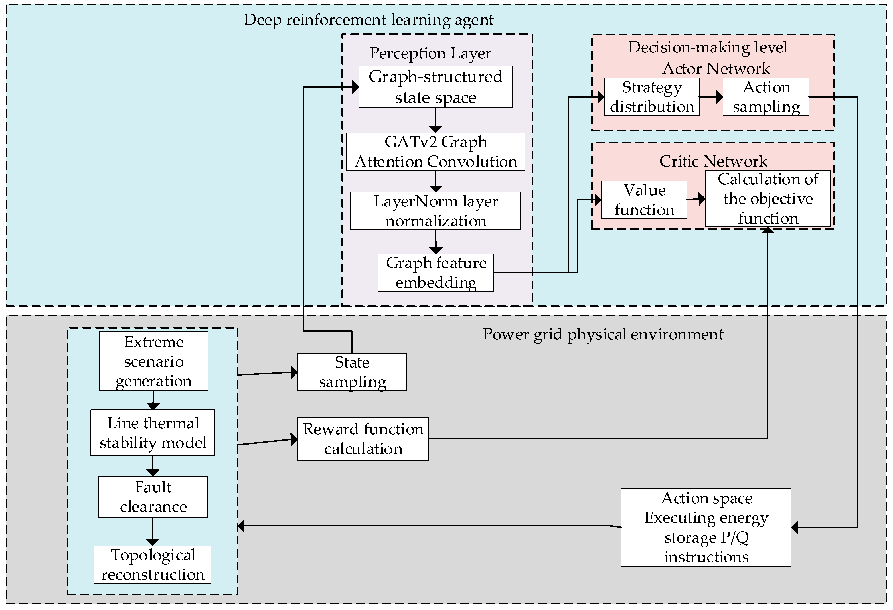
Section 4 completed the screening of candidate energy storage nodes and the three-dimensional coordinated capacity determination of active power, energy, and reactive power. However, the planning results can enhance system resilience only if they are implemented promptly and in a coordinated manner during fault evolution. Under extreme scenarios, cascading failures involve time-varying topology, strong state nonlinearity, and tightly coupled constraints. During fault propagation, line outages, power-flow redistribution, and local islanding continuously reshape the system risk distribution. Conventional control methods based on fixed rules or linear feedback cannot effectively balance overload suppression, voltage support, and ESS energy management. Therefore, this paper develops a multi-ESS coordinated defense framework that integrates graph neural networks with proximal policy optimization. The framework captures changes in network topology and operational risk in a graph-structured state space and outputs coordinated active and reactive power commands for ESS units. Its overall architecture consists of an environment layer, a perception layer, a decision layer, and an execution layer, as shown in Figure 2.

Communication assumptions: To focus on the multi-ESS cooperative control mechanism itself, this study assumes an ideal and reliable communication link between the control center and the energy storage units. Communication constraints such as delays, packet loss, and measurement asynchrony are not explicitly modeled at the current stage.

5.1. Intelligent Collaborative Control Framework Based on Graph Neural Networks

The defense capability of ESSs depends not only on planning-level capacity allocation but also on whether the operational layer can rapidly coordinate multi-node responses based on real-time conditions. Based on the thermal-accumulation-aware cascading-failure model in Section 3 and the ESS allocation results in Section 4, this paper formulates the power-grid environment, ESS units, and fault-propagation process as a graph-structured decision-making problem. Specifically, grid nodes and transmission lines form a time-varying graph, while quantities such as nodal power, voltage, ESS state of charge, and line thermal risk constitute the state features. The graph neural network extracts topology-related representations, and the PPO agent generates coordinated control actions for multiple ESSs, thereby jointly suppressing overload in critical sections and voltage risk in weak areas on a second-level timescale.

5.1.1. Graph-Structured State Space

Considering that during the cascading-failure process, there may be line withdrawals, network decoupling and local topology reconfiguration, the traditional fixed-dimensional vector-based state representation struggles to accurately characterize the connection relationships between nodes and the risk migration process. This paper represents the power grid state at time $t$ as a time-varying graph $G_t=(V,E_t)$, where $V$ is the node set and $E_t$ is the edge set that continuously changes with the fault evolution. The state space $s_t$ is composed of the node feature matrix $X_t$ and the edge feature matrix $E_{ij,t}$. For each node $i$, $X_{i,t}$, the following Equation (41) is constructed:

$$X_{i,t}=\left\{V_{i,t},{\theta }_{i,t},P_{i,t}^{\mathrm{bus}},Q_{i,t}^{\mathrm{bus}},{\mathrm{SOC}}_{\mathrm{ESS},i,t},A_{i,t},D_{i,t},{\mathrm{BESS}}_i\right\}$$

(41)

In the formula, $V_{i,t}$ and ${\theta }_{i,t}$ represent the amplitude and phase angle of the node voltage; $P_{i,t}^{\mathrm{bus}}$ and $Q_{i,t}^{\mathrm{bus}}$ represent the active and reactive power injection at the node; ${\eta }_t$ is the line load rate; ${\mathrm{SOC}}_{\mathrm{ESS},i,t}$ is the state of charge of each energy storage unit; $A_{i,t}$ is the current adjacent topology matrix; $D_{i,t}$ is the node degree; ${\mathrm{BESS}}_i$ is the energy storage installation identifier.

For each line $l_{ij}$, the edge feature matrix $E_{ij,t}$ is constructed as shown in Equation (42):

$$E_{ij,t}=\{{\eta }_{ij,t},R_{ij},X_{ij},T_{ij,t}\}$$

(42)

In the formula, ${\eta }_{ij,t}$ represents the line load rate; $R_{ij},X_{ij}$ represents resistance and reactance; $T_{ij,t}$ represents the real-time temperature of the line.

5.1.2. Multidimensional Discrete Action Space

Considering that PPO is more suitable for stable training in discrete or low-dimensional action spaces and that the actual control instructions of the energy storage system involve the continuous regulation of active and reactive power of multiple units, this paper adopts a multi-dimensional discretization method to encode the control actions of the energy storage system. Assuming there are $N_b$ controllable energy storage units in the system, the action $t$ at time $a_t$ is composed of the active and reactive power adjustment quantities of each energy storage unit, as shown in Equation (43):

$$a_t={\{(P_{i,t},Q_{i,t})\}}_{i=1}^{N_b}$$

(43)

In the formula, $P_{i,t}$ and $Q_{i,t}$ represent the regulation actions for active power and reactive power, respectively.

5.1.3. Reward Function Design

In order to guide the intelligent agent to reduce unnecessary control costs while ensuring system security, this paper constructs a composite reward function including thermal safety, voltage stability, control smoothness and system survivability, as shown in Equation (44):

$$\left\{\begin{array}{l}{r}_t=r_{thermal,t}+r_{voltage,t}+r_{control,t}+r_{survival,t}\\ r_{thermal,t}=-{\lambda }_T{\displaystyle \sum _{l\in L}\max }(0,T_{l,t}-T_{warn})\\ r_{voltage,t}=-{\lambda }_U{\displaystyle \sum _{i=1}^N\max }(0,|U_{i,t}-1.0|-\Delta U_{tol})\\ r_{control,t}=-{\lambda }_P{\displaystyle \sum _{i\in \Phi }|}{P}_{i,t}|-{\lambda }_{\Delta }{\displaystyle \sum _{i\in \Phi }\Vert a_{i,t}-a_{i,t-1}{\Vert }^2}\end{array}\right.$$

(44)

In the formula, $r_{thermal,t}$ represents the thermal safety reward for the line; $T_{warn}$ is the temperature warning threshold; $r_{voltage,t}$ is the voltage stability reward; $U_{i,t}$ is the nominal value of the node voltage; $\Delta U_{tol}$ is the dead zone for the allowable voltage deviation; $r_{control,t}$ is the penalty for action smoothness and energy consumption; $r_{survival,t}$ is the survival reward; and ${\lambda }_T$, ${\lambda }_U$, ${\lambda }_P$ and ${\lambda }_{\Delta }$ are the weighting coefficients for the line thermal accumulation penalty, voltage violation penalty, control smoothness penalty, and SOC limit penalty, respectively. To balance the multiple objectives during the dynamic cascading defense, these weights are empirically tuned and set as follows: ${\lambda }_T=250.0$, ${\lambda }_U=150.0$, ${\lambda }_{\Delta }=30.0$, and ${\lambda }_P=0.01$. Additionally, a positive survival reward of 0.1 is granted for each step the system operates without triggering blackout conditions, thereby encouraging the agent to prolong the secure operational margin.

5.1.4. Network Architecture and Proximal Policy Optimization

To effectively extract the state features of the graph structure and ensure the stability of the training process, this paper constructs a perception network based on Graph Attention Network v2 (GATv2) and Layer Norm and combines it with the PPO algorithm to complete the policy update.

At the perception layer, GATv2 is first utilized to aggregate node features and edge features. Compared to traditional graph attention networks, GATv2 has a more flexible dynamic attention mechanism, which can more sensitively capture the impact of key routes and high-risk nodes on the global state after a fault. Subsequently, Layer Norm is introduced after the convolution layer output to normalize features of different dimensions such as voltage, power, and temperature, in order to alleviate the problems of numerical instability and gradient fluctuations. Finally, through global pooling operations, the updated node embeddings are aggregated into graph-level representations, serving as the shared input for the Actor network and the Critic network.

At the decision-making level, PPO is used to update the parameters of the policy network. PPO introduces a clipping objective function to limit the update range between the old and new policies. The objective function is shown in Equation (45), thereby avoiding performance fluctuations during the training process due to excessive policy updates.

$$L^{CLIP}(\theta )={\widehat{\mathbb{E}}}_t\left[\min (r_t(\theta ){\widehat{A}}_t,\mathrm{clip}(r_t(\theta ),1-ϵ,1+ϵ){\widehat{A}}_t)\right]$$

(45)

In the formula, $\theta$ represents the parameters of the policy network; ${\widehat{E}}_t$ indicates the expected value at time step $t$; $r_t(\theta )={\displaystyle \frac{{\pi }_{\theta }(a_t|s_t)}{{\pi }_{{\theta }_{old}}(a_t|s_t)}}$ is the probability ratio of the old and new policies; ${\widehat{A}}_t$ is the generalized advantage estimation; $ϵ$ is the clipping hyperparameter.

Taking into account strategy optimization, value function fitting and exploration ability, the overall loss function is defined as shown in Equation (46). By minimizing this loss, the Actor and Critic networks can simultaneously complete parameter updates, and gradually learn to acquire multi-energy storage collaborative control strategies applicable to complex extreme scenarios.

$$L_{total}=-L^{CLIP}(\theta )+c_1{L}^{VF}(\varphi )-c_{2}S[{\pi }_{\theta }](s_t)$$

(46)

In the formula, $L^{VF}(\varphi )={(V_{\varphi }(s_t)-V_t^{target})}^2$ represents the mean square error loss of the value network; $S[{\pi }_{\theta }]$ represents the policy entropy; $c_1,c_2$ represents the weight coefficient for balancing the losses of all items.

5.2. Agent-Driven Collaborative Defense Process for Cascading Failures

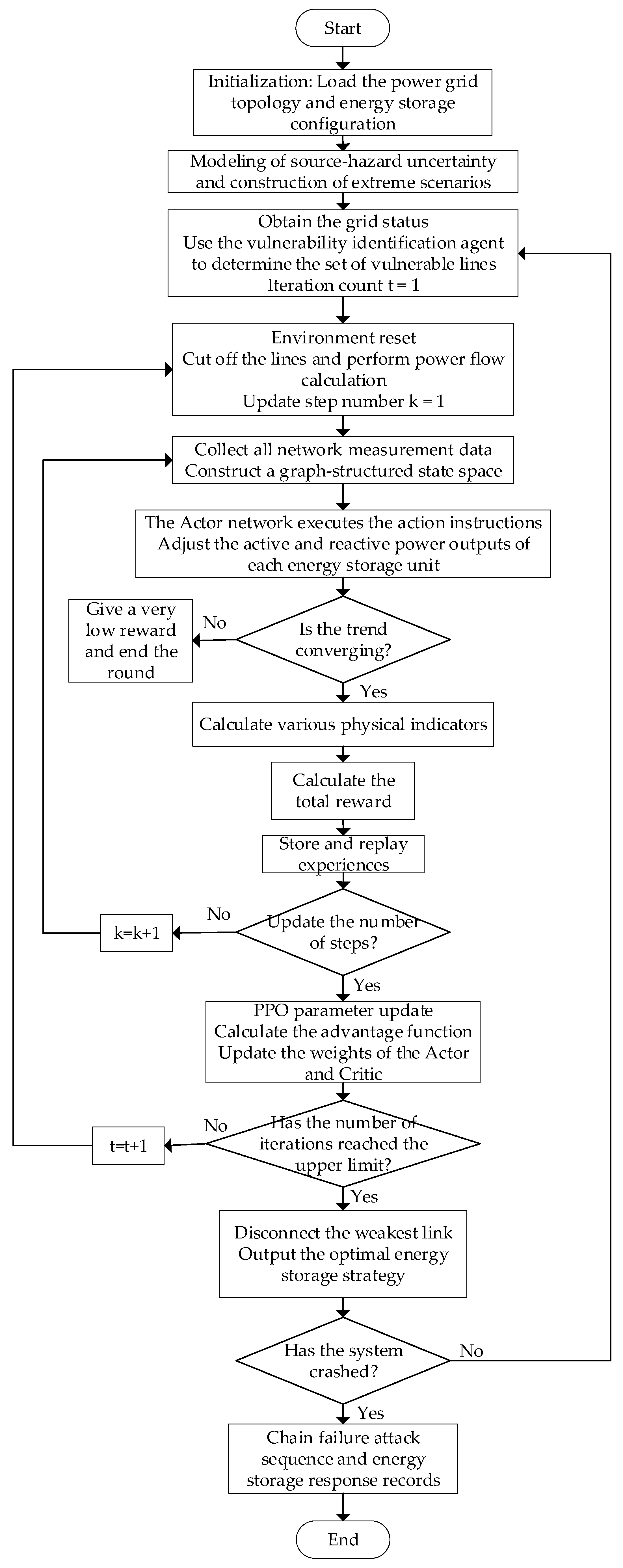
After strategy training is completed, an offline-training/online-defense closed-loop process is established, as shown in Figure 3. The process first generates extreme scenarios based on the source-load uncertainty model and uses the vulnerability-identification results from Section 3 to determine the high-risk fault set. During training, the complexity of fault scenarios is gradually increased through curriculum learning, and the agent continuously collects measurement data from the power grid environment to construct a graph-structured state and output energy storage active and reactive control instructions; the environment layer then performs power flow calculation, thermal stability verification, and voltage safety verification based on this, and feeds back the rewards to PPO for strategy update.

During the online defense stage, when the system encounters initial disturbances in critical lines or cascading failures, the intelligent agent quickly generates the optimal energy storage response strategy based on the real-time graph state. This strategy, on the one hand, suppresses the continuous overload and temperature rise accumulation at the critical sections through active power regulation, and on the other hand, stabilizes the voltage in the local weak areas through reactive power support, thereby delaying the fault propagation and reducing the risks of system separation and load loss. As the fault evolves, the intelligent agent continues to output control actions iteratively based on the updated topology and state until the system returns to stability or the fault process ends.

Compared with traditional static defense methods, this closed-loop process achieves the integration of the risk identification in Section 3, the energy storage configuration in Section 4, and the online collaborative control in this section. Its core lies not in the local optimization at a single moment but in the dynamic defense for the entire fault process. This enables the energy storage resources to continuously respond over time, collaboratively cover in space, and simultaneously perform overload suppression and voltage support functions. Ultimately, it forms a collaborative defense chain for extreme scenario cascading failures.

6. Calculation Examples

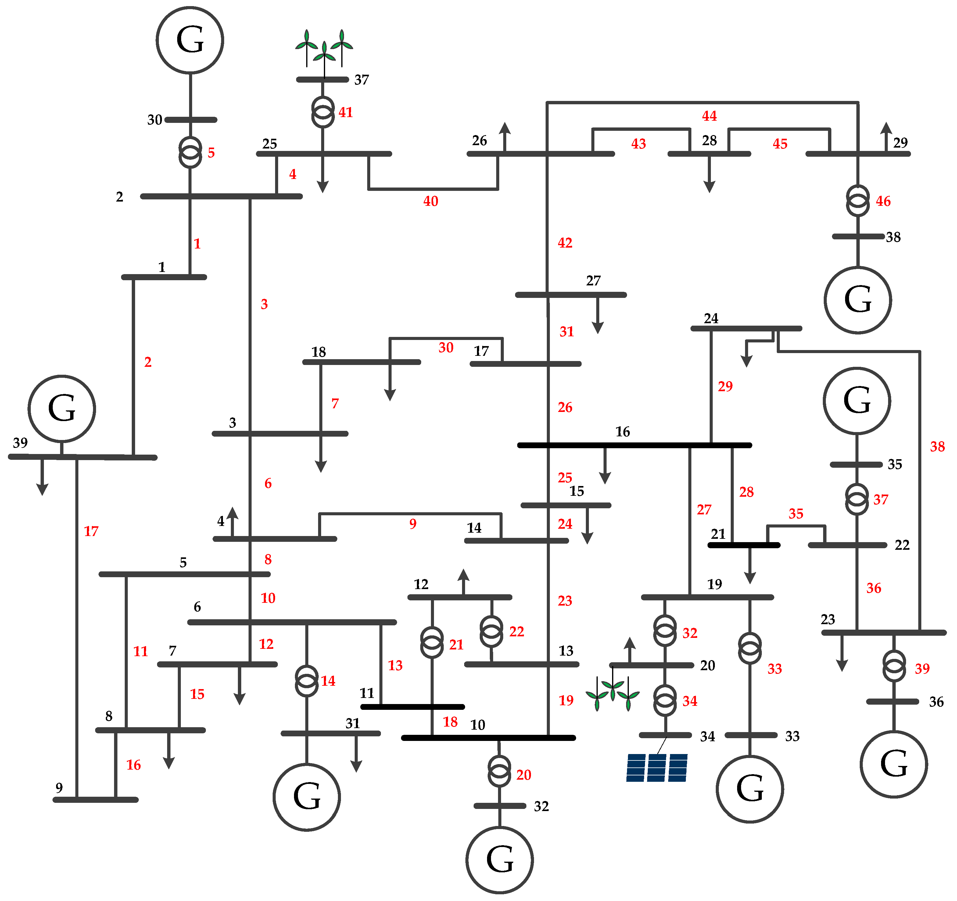
To verify the effectiveness of the proposed framework for dynamic vulnerability identification, hierarchical ESS planning, and intelligent coordinated control, case studies were conducted on a modified IEEE 39-bus system, as shown in Figure 4. In Figure 4, the red numbers denote line numbers, and the black numbers denote bus numbers. To reflect a high level of renewable penetration, buses 34 and 37 were replaced by an equal-capacity photovoltaic plant and a wind farm, respectively, and an additional 300 MW wind farm was connected to bus 20. To maintain system power balance, the outputs of conventional units G09 and G10 were reduced accordingly. The model was implemented in Python 3.8. Grid modeling and power-flow calculation were carried out in pandapower 2.14.11, and the policy network was implemented in PyTorch 2.4.1+cu124. The total training horizon of the GNN-PPO agent was 3 × 10⁶ timesteps. The discount factor was 0.99, the learning rate was 3 × 10⁻⁴, the number of sampling steps per update was 1024, the batch size was 64, and each update was repeated 10 times. The entropy regularization coefficient was set to 0.01. Offline training and online evaluation were performed on a computer equipped with an AMD Ryzen 7940H CPU and an NVIDIA RTX 4060 GPU. The offline training process required approximately 10 h. During online execution, each dynamic fault scenario was completed within 0.35 s, which satisfies the real-time requirements of emergency cascading-failure defense.

6.1. Identification Results of Grid Vulnerability

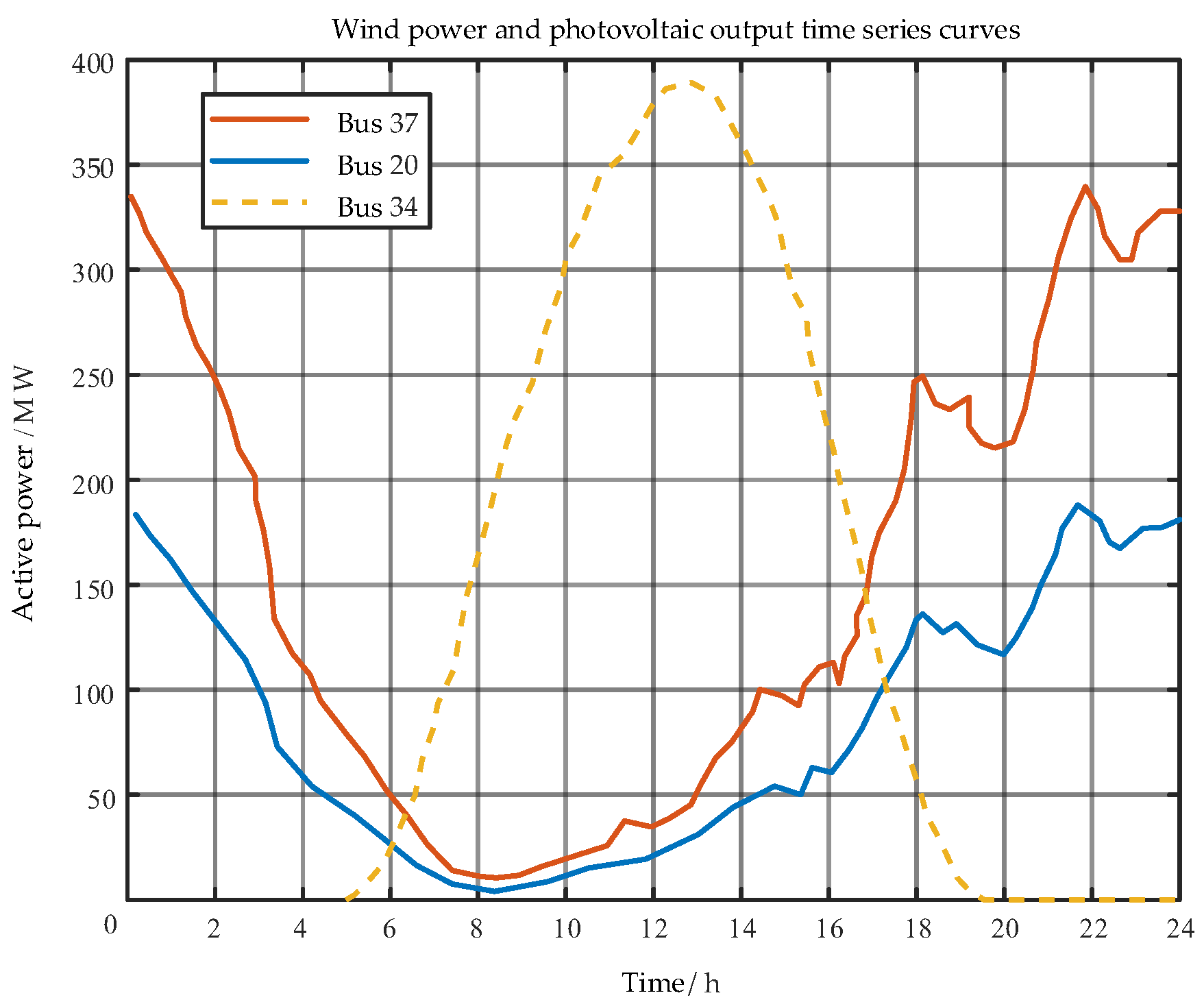
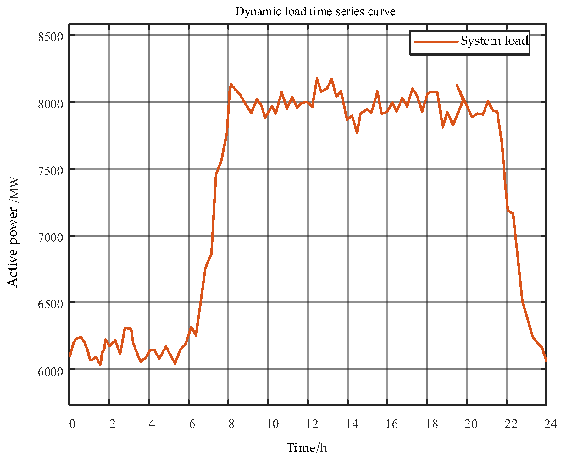
Based on the source-load uncertainty model constructed in Section 3.1.1, time-series curves for wind power, photovoltaic power, and dynamic loads were generated, as shown in Figure 5 and Figure 6, respectively. The corresponding samples contain random fluctuation characteristics and can be used as input for extracting subsequent extreme scenarios.

Figure 5 and Figure 6 are mainly used to illustrate the randomness and correlation of the source-load sample library. They are not intended as the final comparative results of control performance. Based on these time-series samples, typical operating points are extracted according to seven indicators: maximum net load, minimum net load, maximum renewable output, maximum wind output, maximum photovoltaic output, maximum ramp rate, and worst-case voltage.

The simulation selects 7 typical scenarios covering extreme source-grid-load states, specifically including the maximum net load (Scenario 1), minimum net load (Scenario 2), maximum renewable generation output (Scenario 3), maximum wind power output (Scenario 4), maximum photovoltaic power output (Scenario 5), maximum ramping rate (Scenario 6), and worst-case voltage condition (Scenario 7).

Under these scenarios, this paper constructs a fault sample set, performs batch cascading-failure simulations, and statistically analyzes the key fault sequences and their dynamic vulnerability scores.

Table 2. The evolutionary sequence of cascading failures in extreme scenarios and the proximity degree of dynamic vulnerability.

Scenario Number	Chain Failure Evolution Sequence	Dynamic Vulnerability Proximity
1	L5-6, L6-7, L13-14	[0.676, 0.852, 0.894]
2	L6-11, L10-13, L13-14	[0.759, 0.821, 0.883]
3	L8-9, L16-24, L21-22	[0.768, 0.816, 0.988]
4	L9-39, L21-22, L16-19	[0.652, 0.804, 0.847]
5	L20-34, L19-20, L16-19	[0.939, 0.951, 0.982]
6	L8-9, L21-22, L17-27	[0.592, 0.672, 0.887]
7	L15-16, L16-17, L17-27	[0.735, 0.844, 0.886]

presents the chain fault sequences with the highest threat ranking and the corresponding proximity in each scenario. The results show that, in multi-stage fault sequences, the vulnerability proximity of subsequently disconnected lines generally increases. This indicates that power-flow redistribution caused by the initial disturbance continuously erodes the remaining safety margin of the system and drives the fault chain toward more vulnerable topological links. Thus, critical vulnerable branches are not fixed; they vary with both the operating scenario and the stage of fault evolution.

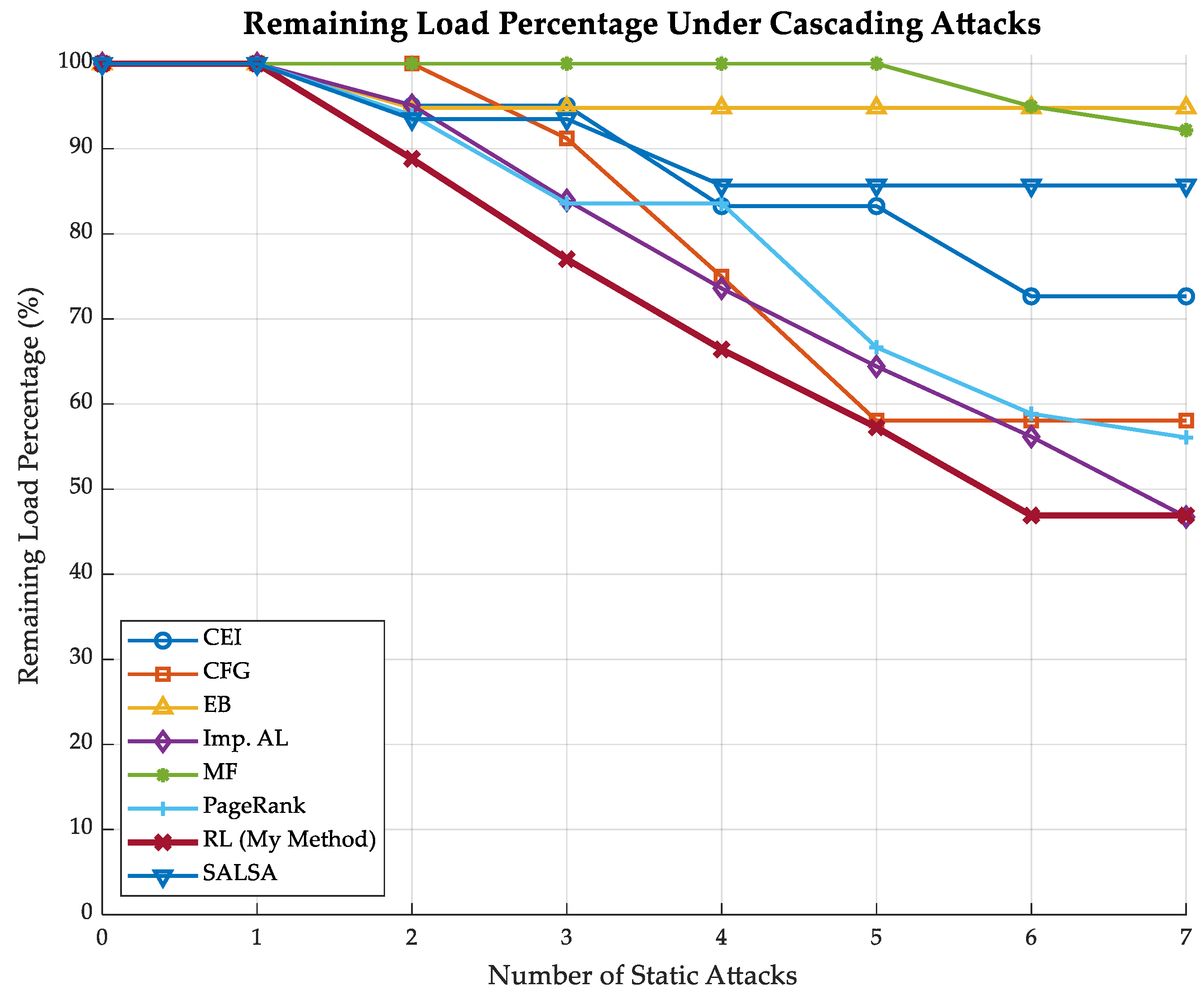
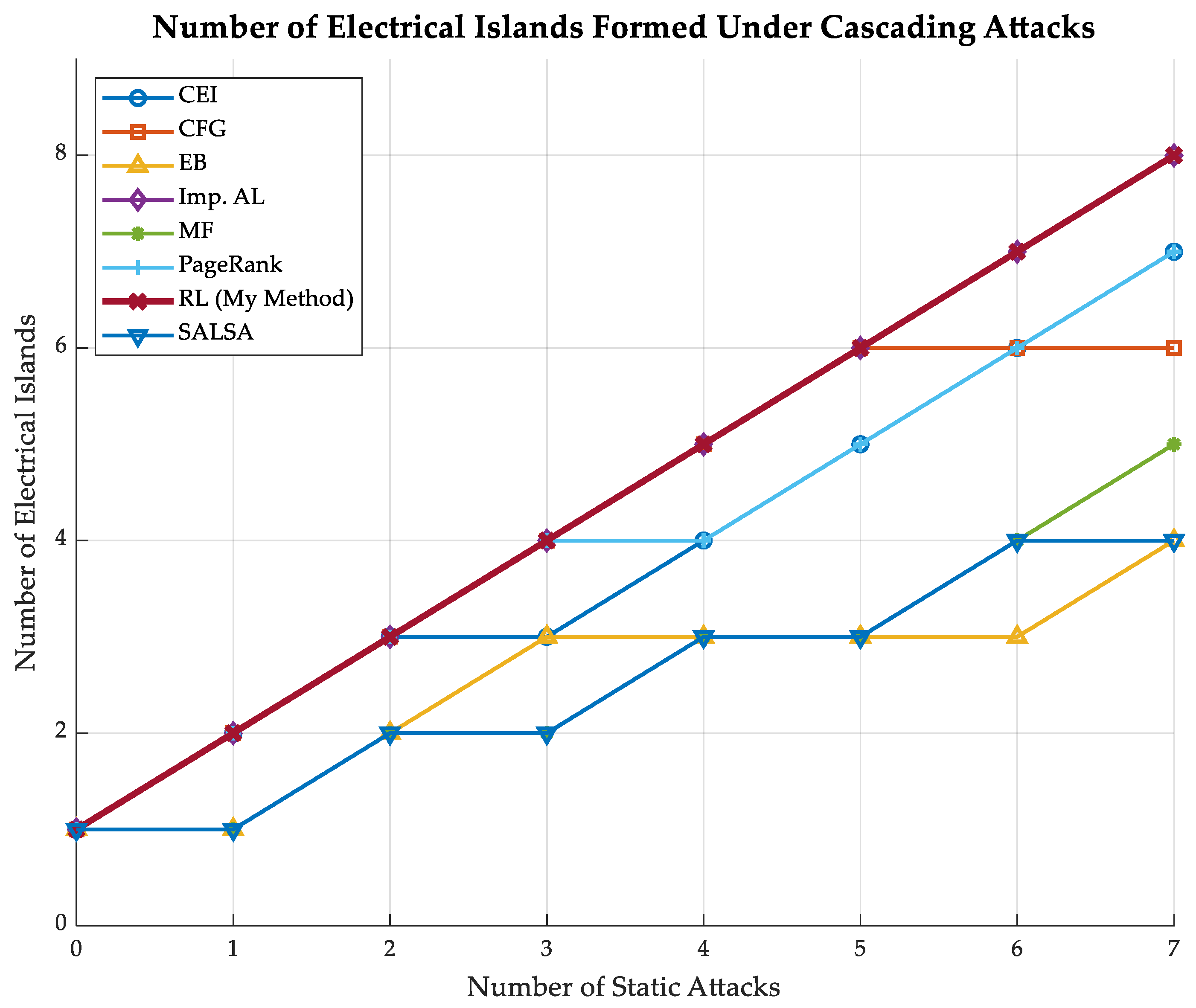
Figure 7 compares the decline in residual load ratio under continuous line removal for different identification methods. When the line sequence identified by the proposed method is removed, the residual load ratio decreases most rapidly, eventually reaching 46.1%, which is lower than that obtained with PageRank and CEI. This result indicates that the proposed method more accurately identifies branches that have a decisive effect on system supply capability. Figure 8 further shows that the proposed method leads to the formation of eight electrical islands, indicating a higher degree of topological fragmentation and a stronger ability to uncover deep vulnerable structures.

6.2. Energy Storage Configuration Results

After identifying the key vulnerable branches and their temporal–spatial distribution, this paper further maps line risks to candidate ESS deployment areas and installation nodes using the hierarchical planning method proposed in Section 4. First, the Louvain algorithm partitions the modified IEEE 39-bus system into communities with strong electrical coupling. Then, key hub nodes are selected from each zone based on electrical betweenness to form the candidate set, as summarized in

Table 3. Community partition results and candidate buses.

Community ID	Nodes Included in the Community	The Selected Nodes	Electrical Connectivity Score
0	[25, 37]	25	0.474
1	[1, 39]	39	0.273
2	[8, 9]	8	0.362
3	[3, 18]	3	0.583
4	[26, 28, 29, 38]	26	0.508
5	[11, 10, 32]	10	0.283
6	[17, 27]	17	0.683
7	[4, 5]	4	0.510
8	[16, 19, 20, 33, 34]	16	1.000
9	[21, 22, 35]	21	0.237
10	[24, 23, 36]	24	0.197
11	[2, 30]	2	0.637
12	[6, 7, 31]	6	0.420
13	[14, 13, 15, 12]	14	0.485

.

The final set of candidate nodes is: {2, 3, 4, 6, 8, 10, 14, 16, 17, 21, 24, 25, 26, 39}. This result ensures that the energy storage layout covers the key areas spatially and avoids excessive concentration of defense resources.

Based on this, the NSGA-II algorithm was used to solve the three-dimensional collaborative capacity allocation model constructed in Section 4, and the energy storage configuration scheme shown in

Table 4. Configuration scheme of energy storage systems.

Bus Number	Rated Power P (MW)	Rated Energy E (MWh)	Rated Reactive Power Capacity Q (MVar)
2	75.0	25.0	30.0
3	240.0	65.0	35.0
4	215.0	65.0	30.0
6	100.0	35.0	30.0
8	155.0	40.0	30.0
10	130.0	40.0	25.0
14	110.0	35.0	30.0
16	125.0	35.0	50.0
17	120.0	30.0	30.0
21	200.0	50.0	55.0
24	120.0	40.0	50.0
25	140.0	45.0	15.0
26	110.0	30.0	15.0
39	115.0	30.0	15.0

was obtained.

The results show clear functional differences among nodes in terms of active power, energy, and reactive power configuration. Nodes 3, 4, and 21 are located near critical power-flow corridors and therefore receive larger active-power ratings, indicating their role in peak shaving and load relief during the early stage of faults. Nodes 16, 21, and 24 are located near renewable-rich areas or weak-voltage areas and therefore receive a higher share of reactive-power capacity, reflecting the model’s emphasis on local voltage support. Some nodes are assigned larger energy capacities to ensure sustained support during prolonged fault evolution and local islanding. Overall, the configuration demonstrates complementary allocation of active power, energy, and reactive power, and shows that three-dimensional coordinated planning is better suited to cascading-failure defense than single-capacity planning.

6.3. Analysis of the Cooperative Defense Effect of Chain Failures Under Energy Storage Participation

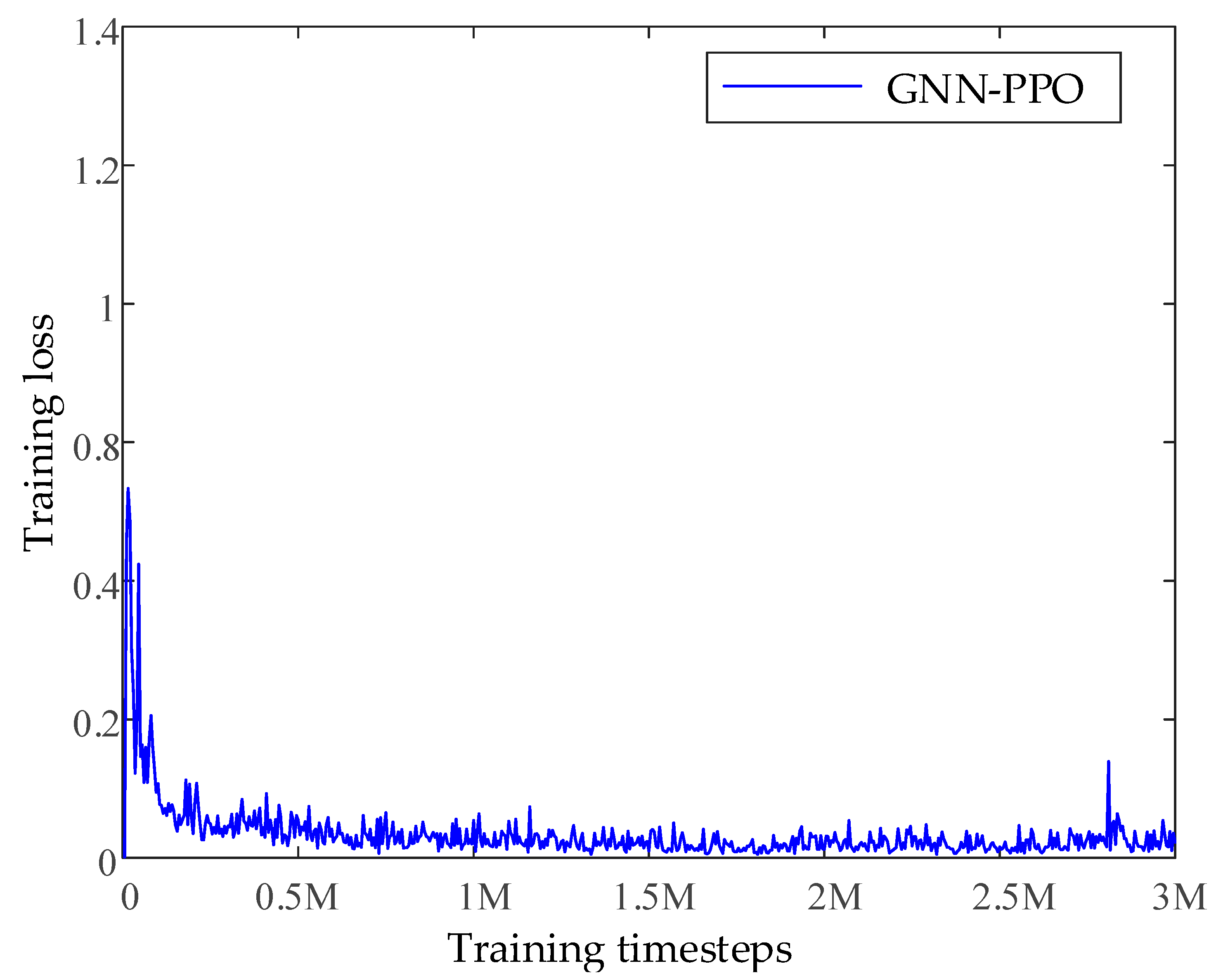
As shown by the training-loss curve in Figure 9, the horizontal axis denotes the training timesteps, and the vertical axis denotes the loss value. The loss decreases rapidly during the initial exploration phase and converges to a stable region by approximately 3 × 10⁶ timesteps, demonstrating the stable learning capability of the graph-structured policy under complex fault scenarios.

After the physical ESS configuration was completed, the online defense performance of the GNN-PPO-based coordinated control strategy was further evaluated during fault evolution. The outage of line L7 was selected as the initial triggering event. Under this scenario, the system operated at a relatively high load level. Without effective intervention, the outage of L7 would rapidly redistribute power flow, causing continuous overload in key lines such as L27 and driving the system into a thermal-accumulation risk region.

Table 5. Evolution of cascading failures with ESS participation.

Evolutionary Stage	Faulty Line	Critical Risk Profile	Main Energy Storage Response	Defensive Effect
Phase 1 t = 0 s	L7	L27 overload 123.35%	Bus 4: 112.1 MW	The load rate has decreased to 105.13%
			Bus 26: 106.9 MW
			Bus 8: 101.0 MW
			Bus 17: 73.1 MW
Phase 2 t = 300 s	L13	L27 overload 137.31%	Bus 4: 132.9 MW	The load rate has decreased to 108.29%
			Bus 6: 100.0 MW
			Bus 8: 131.9 MW
			Bus 39: 80.3 MW
Phase 3 t = 600 s	L19	L21 overload 129.99%	Bus 8: 96.9 MW	The load rate has decreased to 114.43%
			Bus 4: 107.4 MW
			Bus 6: 98.8 MW
			Bus 3: 69.4 MW
Phase 4 t = 900 s	L3	L18 overload 116.73%	Bus 3: 79.2 MW	The load rate has decreased to 114.43%
			Bus 4: 74.8 MW
			Bus 8: 88.3 MW
			Bus 14: 54.2 MW
Phase 5 t = 1200 s	L8	L25 overload 151.07%	Bus 3: 209.6 MW	The system maintains critical stability
			Bus 4: 215.0 MW
			Bus 14: 110.0 MW
			Bus 10: 130.0 MW

summarizes the cascading-failure evolution process with ESS participation.

In the first stage, following the tripping of the initial faulty line L7, the loading of L27 increased rapidly. The intelligent agent identified the energy storage nodes that had a significant impact on this section based on the current graph state, and organized multi-node coordinated output to implement active power peak shaving for the critical channel, thereby reducing the load rate of L27 from the high-risk zone to close to the safety boundary. This result indicates that energy storage can utilize the intervention window formed by thermal inertia in the early stage of the fault to provide rapid support for the critical lines, delaying subsequent tripping.

During the second to fourth stages, although the critical section risks from the previous stage were alleviated, as the system topology weakened, the overload risks gradually shifted to other lines. The system successively experienced the withdrawal of L13, L19, and L3. In the face of the constantly changing topology and overload locations, the intelligent agent did not maintain a fixed control mode. Instead, it continuously adjusted the main supporting nodes based on the real-time status, allowing the center of energy storage output to dynamically shift along with the migration of risk sections. This shows that the proposed method does not aim to rigidly suppress all local disturbances. Instead, it dynamically coordinates limited energy storage resources to prioritize maintaining the backbone grid and key power supply capabilities.

In the fifth stage, after line L8 was disconnected, L25 experienced further overload. At this point, multiple ESS units became capacity-constrained, and the overall system support capability approached its rated limit. Although the extreme overload was not completely eliminated, the system remained in a critically stable state and did not immediately evolve into an uncontrollable collapse. This provided additional time for subsequent breaker actions or load-shedding measures. These results indicate that the proposed strategy remains robust even in highly complex scenarios and can shift the defense objective from completely blocking all faults to prioritizing system survivability and reducing outage consequences.

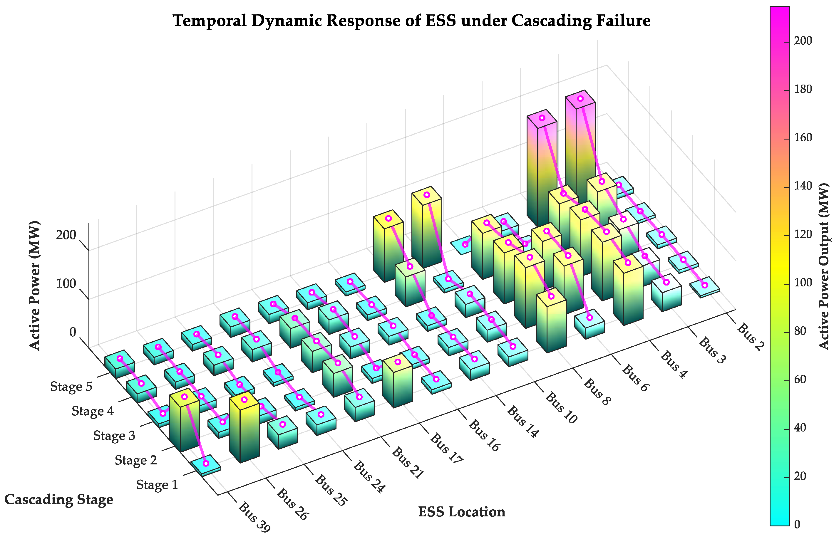
To further illustrate the spatiotemporal characteristics of coordinated defense, Figure 10 presents the three-dimensional distribution of active-power output for the 14 ESS nodes throughout the cascading-failure process. The ESS units do not respond simultaneously or proportionally. Instead, their output exhibits clear spatial shifts and intensity redistribution as the failure stage progresses. Key nodes assume a dominant supporting role during high-risk periods, while other nodes provide background support and local compensation. This behavior demonstrates the spatial hierarchy, temporal continuity, and functional coordination of the proposed method.

6.4. Baseline Comparison, Statistical Evaluation, and Sensitivity Analysis

• Baseline comparison and statistical evaluation

To validate the superiority and robustness of the proposed framework, a comprehensive statistical comparison is conducted between the proposed GNN-PPO strategy and a conventional Sensitivity-Based Control (SBC) baseline. The conventional SBC strictly relies on static numerical sensitivities (e.g., PTDF) to dispatch local ESSs, fundamentally lacking global graph-topology awareness and multi-layer coordination.

To evaluate performance under highly stochastic operating conditions, a Monte Carlo simulation was implemented. Gaussian white noise (±10% fluctuation) was superimposed on the source-load profiles to generate N = 10 randomized extreme operational seeds. The statistical comparison results are comprehensively summarized in

Table 6. Statistical comparison between the conventional SBC and the proposed GNN-PPO framework (N = 10).

Evaluation Metric	Conventional SBC (Baseline)	Proposed GNN-PPO	Improvement (%)
Maximum Line Loading (%)	236.41 ± 26.53	176.53 ± 19.88	+25.33%
Minimum Bus Voltage (p.u.)	0.8514 ± 0.0860	0.8752 ± 0.0601	+2.80%
Survived Cascading Stages	3.80 ± 0.79	4.80 ± 0.63	+26.32%

.

As demonstrated in Table 6, under equivalent extreme cascading fault scenarios, the proposed GNN-PPO framework significantly outperforms the conventional SBC method across all critical metrics. By introducing global topological awareness, the proposed method reduces the maximum line thermal stress by 25.33% and narrows its standard deviation (from 26.53 to 19.88), indicating much more stable flow control under stochastic noise. Furthermore, the GNN-PPO framework’s dynamic active/reactive coordination successfully mitigates local voltage dips, increasing the average number of cascading stages survived from 3.80 to 4.80, which corresponds to a 26.32% improvement in system survivability.

2.

Sensitivity analysis

A sensitivity analysis was conducted with respect to renewable-energy penetration. The renewable-penetration factor was increased from the baseline case (Scale = 1.0) to more extreme low-inertia conditions (Scale = 1.66 and 2.0). Under the baseline scale, the system survived four cascading stages, with a maximum loading of 162.25%. When renewable penetration doubled (Scale = 2.0), overall system inertia decreased substantially, accelerating fault propagation. Nevertheless, under the continuous spatial regulation of the GNN-PPO agent, dynamic reactive-power support effectively compensated for voltage instability. Even at Scale = 2.0, the system survived four critical cascading stages without total blackout, although the maximum line loading increased to 225.58%. These results confirm the adaptability and robustness of the proposed multi-ESS framework under extremely high renewable penetration.

7. Conclusions

This study addresses cascading-failure defense in renewable-dominated power grids under extreme operating scenarios and develops a closed-loop framework for dynamic vulnerability identification, hierarchical ESS planning, and online coordinated defense, reaching the following conclusions:

• Based on the uncertainties of wind power, photovoltaic generation, and load, seven typical extreme operating scenarios are extracted. A cascading-failure evolution model that considers conductor thermal accumulation and protection actions is then established, and TOPSIS is employed to comprehensively identify critical vulnerable branches. The results show that system vulnerabilities are scenario-dependent and migrate dynamically during fault evolution.
• By combining community partitioning with electrical-betweenness screening, a three-dimensional coordinated ESS configuration model is developed for active power, energy capacity, and reactive power support. This model enables hierarchical siting and differentiated capacity allocation. The results show that different nodes assume distinct functions, including active power peak shaving, sustained energy support, and local voltage regulation, during fault defense.
• A graph-neural-network- and PPO-based multi-ESS coordinated defense strategy is further proposed. It incorporates topological changes, line-temperature rise, voltage risk, and ESS operating status into the decision-making process. Case studies show that the proposed method dynamically adjusts ESS outputs according to evolving risk locations, reduces line-overload accumulation, mitigates voltage risk, and improves system survivability.

Overall, this study verifies the effectiveness of an integrated ‘identification-allocation-control’ closed-loop defense chain for cascading failures under extreme operating scenarios. Future work will extend the present framework to larger-scale transmission systems and more complex operating conditions in order to further assess its robustness and engineering applicability.

References

1. Tu, J.; He, J.; An, X.; Zhang, G.; Xie, Y.; Sun, W.; Li, L. Analysis and lessons of Pakistan blackout event on January 23, 2023. Proc. CSEE 2023, 43, 5319–5329. [Google Scholar]
2. Yan, D.; Wen, J.; Du, Z.; Yang, D. Analysis of Texas blackout in 2021 and its enlightenment to power system planning management. Power Syst. Prot. Control 2021, 49, 121–128. [Google Scholar]
3. Zhang, P.; Ma, C.; Li, W.; Ma, H.; Liu, S.; Fan, J. Analysis of two splitting accidents of European power grid in 2021 and consideration on power grid security in China. Autom. Electr. Power Syst. 2021, 45, 22–29. [Google Scholar]
4. Sun, H.; Xu, T.; Guo, Q.; Li, Y.; Lin, W.; Yi, J.; Li, W. Analysis on blackout in Great Britain power grid on August 9, 2019 and its enlightenment to power grid in China. Proc. CSEE 2019, 39, 6183–6192. [Google Scholar]
5. Hu, P.; Mei, T.; Fan, W. Cascading failure forecast of complex power grids: A review. Sci. Sin. Technol. 2017, 47, 355–363. [Google Scholar] [CrossRef] [Scilit]
6. Guo, Z.; Sun, K.; Su, X.; Simunovic, S. A review on simulation models of cascading failures in power systems. iEnergy 2023, 2, 284–296. [Google Scholar] [CrossRef] [Scilit]
7. Bai, J.; Liu, T.; Cao, G.; Chen, C. A survey on vulnerability assessment method for power system. Power Syst. Technol. 2008, 32, 26–30. [Google Scholar]
8. Lin, P.; Wu, J.; Huang, T.; Lei, X.; Jia, Y.; Wu, Y. Overview of vulnerability assessment for power systems. Smart Power 2021, 49, 22–28. [Google Scholar]
9. Zhou, K.; Dobson, I.; Wang, Z.; Roitershtein, A.; Ghosh, A.P. A Markovian influence graph formed from utility line outage data to mitigate large cascades. IEEE Trans. Power Syst. 2020, 35, 3224–3235. [Google Scholar] [CrossRef] [Scilit]
10. Khodadadi Arpanahi, M.; Capitanescu, F. A new comprehensive framework for cascading outage simulation in power systems. Electr. Power Syst. Res. 2024, 234, 110624. [Google Scholar] [CrossRef] [Scilit]
11. Ghosh, S.S.; Dwivedi, A.; Tajer, A.; Yeo, K.; Gifford, W.M. Cascading failure prediction via causal inference. IEEE Trans. Power Syst. 2024, 40, 3361–3373. [Google Scholar] [CrossRef] [Scilit]
12. Wu, X.; Cao, Y.; Wu, H.; Qi, S.; Zhao, M.; Feng, Y.; Yu, Q. Hybrid learning-based fault prediction and cascading failure mitigation in multi-network energy systems. Sci. Rep. 2025, 15, 33938. [Google Scholar] [CrossRef] [Scilit] [PubMed]
13. Zakeri, B.; Syri, S. Electrical energy storage systems: A comparative life cycle cost analysis. Renew. Sustain. Energy Rev. 2015, 42, 569–596. [Google Scholar] [CrossRef] [Scilit]
14. Yang, B.; Wang, J.; Chen, Y.; Li, D.; Zeng, C.; Chen, Y.; Guo, Z.; Shu, H.; Zhang, X.; Yu, T.; et al. Optimal sizing and placement of energy storage system in power grids: A state-of-the-art one-stop handbook. J. Energy Storage 2020, 32, 101814. [Google Scholar] [CrossRef] [Scilit]
15. Yang, B.; Liu, X.; Tian, Z.; Zhang, Y.; Lan, L.; Lu, H. Comprehensive vulnerability-driven energy-storage optimal allocation and disaster-resilience analysis for distribution networks. High Volt. Eng. 2025, 51, 5078–5089. [Google Scholar]
16. Wang, Q.; Shi, B.; Chi, Y.; Zhou, Y.; Zhang, C.; Zhou, N. Adaptive coordinated planning of energy storage for low-inertia power systems based on dynamic frequency security assessment. Autom. Electr. Power Syst. 2026, 50, 165–185. [Google Scholar]
17. Hu, J.; Gao, L.; Cui, S.; Ai, X.; Li, K.; Li, G.; Tang, W.; Fang, J.; Cao, Y.; Wen, J. Optimal scheduling method of power system considering coordinated frequency support of flywheel and lithium-ion battery energy storage. Electr. Power Autom. Equip. 2026, 46, 23–32. [Google Scholar]
18. Yu, P.; Xiong, X.; Zhu, J.; He, X.; Nan, D. Active prevention and control method against power grid cascading tripping based on participation of energy storage. Autom. Electr. Power Syst. 2024, 48, 119–130. [Google Scholar]
19. Espina, E.; Cárdenas-Dobson, R.J.; Simpson-Porco, J.W.; Kazerani, M.; Sáez, D. A consensus-based distributed secondary control optimization strategy for hybrid microgrids. IEEE Trans. Smart Grid 2023, 14, 4242–4255. [Google Scholar] [CrossRef] [Scilit]
20. Yang, C.; Zheng, T.; Bu, M.; Li, P. A communication-saving distributed secondary control of hybrid AC/DC microgrids and its small-signal analysis. Electr. Power Syst. Res. 2024, 229, 110186. [Google Scholar] [CrossRef] [Scilit]
21. Salman, M.; Ling, Y.; Li, Y.; Xiang, J. Coordination-based power management strategy for hybrid AC/DC microgrid. IEEE Syst. J. 2023, 17, 6528–6539. [Google Scholar] [CrossRef] [Scilit]
22. Mahmoudian, A.; Garmabdari, R.; Bai, F.; Guerrero, J.M.; Mousavizade, M.; Lu, J. Adaptive power-sharing strategy in hybrid AC/DC microgrid for enhancing voltage and frequency regulation. Int. J. Electr. Power Energy Syst. 2024, 156, 109696. [Google Scholar] [CrossRef] [Scilit]
23. Huang, W.; Zhang, X.; Li, K.; Zhang, N.; Strbac, G.; Kang, C. Resilience Oriented Planning of Urban Multi-Energy Systems With Generalized Energy Storage Sources. IEEE Trans. Power Syst. 2022, 37, 2906–2918. [Google Scholar] [CrossRef] [Scilit]
24. Mishra, D.K.; Ghadi, M.J.; Li, L.; Zhang, J.; Hossain, M.J. Active distribution system resilience quantification and enhancement through multi-microgrid and mobile energy storage. Appl. Energy 2022, 311, 118665. [Google Scholar] [CrossRef] [Scilit]
25. Oikonomou, K.; Maloney, P.R.; Bhattacharya, S.; Holzer, J.T.; Anderson, O.; Ke, X.; Westman, J.; Burleyson, C.D.; Datta, S.; Twitchell, J.B.; et al. Energy storage planning for enhanced resilience of power systems against wildfires and heatwaves. J. Energy Storage 2025, 119, 116074. [Google Scholar] [CrossRef] [Scilit]
26. Yuan, H.; Shen, Y.; Xie, X. A novel robust optimization method for mobile energy storage pre-positioning. Appl. Energy 2025, 379, 124810. [Google Scholar] [CrossRef] [Scilit]
27. Peng, Z.; Xu, Y.; Xie, Z.; Sun, W.; Qi, W.; Zhou, X.; Wu, Q. Analysis of frequency characteristics for new power system considering coordinated participation of multi-type energy storage. Distrib. Energy 2026, 11, 83–93. [Google Scholar]
28. Huang, Q.; Huang, R.; Hao, W.; Tan, J.; Fan, R.; Huang, Z. Adaptive power system emergency control using deep reinforcement learning. IEEE Trans. Smart Grid 2020, 11, 1171–1182. [Google Scholar] [CrossRef] [Scilit]
29. Hu, Z.; Shi, Z.; Zeng, L.; Yao, W.; Tang, Y.; Wen, J. Knowledge-enhanced deep reinforcement learning for intelligent event-based load shedding. Int. J. Electr. Power Energy Syst. 2023, 148, 108978. [Google Scholar] [CrossRef] [Scilit]
30. Zhang, X.; Wang, Q.; Bi, X.; Li, D.; Liu, D.; Yu, Y.; Tse, C.K. Mitigating cascading failure in power grids with deep reinforcement learning-based remedial actions. Reliab. Eng. Syst. Saf. 2024, 250, 110242. [Google Scholar] [CrossRef] [Scilit]
31. Wang, B.; Tang, Y.; Huang, Y.; Wang, T. Power system emergency control strategy based on severely disturbed units identification and STGCN-DDQN. Electr. Power Syst. Res. 2024, 226, 109903. [Google Scholar] [CrossRef] [Scilit]
Figure 1. The typical evolution chain and intervention window of cascading failures in extreme scenarios.
Energies 19 01944 g001
Figure 2. Architecture diagram of the intelligent agent model.
Energies 19 01944 g002
Figure 3. Flowchart of cascading failure defense based on agent reinforcement learning.
Energies 19 01944 g003
Figure 4. Modified IEEE 39-bus system.
Energies 19 01944 g004
Figure 5. Time-series output curves of wind power and PV generation.
Energies 19 01944 g005
Figure 6. Time-series curves of dynamic load.
Energies 19 01944 g006
Figure 7. Trend of residual load ratio.
Energies 19 01944 g007
Figure 8. Trend of the number of electrical islands.
Energies 19 01944 g008
Figure 9. Training loss curve.
Energies 19 01944 g009
Figure 10. Three-dimensional bar chart of ESS power output.
Energies 19 01944 g010