Forecasting–Scheduling Co-Optimization for Rural Microgrids: An Edge-Deployable Approach

Abstract

The high penetration of distributed renewable energy in rural microgrids imposes severe physical-layer fluctuations, weak information-layer communication, and limited computing-layer resources. These triple constraints create a fundamental tension: high-precision forecasting and real-time scheduling are required, yet edge devices face severe resource limitations. To resolve this, we present an edge-deployable energy management system (EMS) that achieves forecasting–scheduling co-optimization. We first propose an Adaptive Gated Dual-stream Network (AGDN), which employs a feature-dimension gated fusion mechanism to overcome the limitations of the local dependency strengths of Long Short-Term Memory (LSTM) and the global perception capabilities of Transformer models under volatile rural conditions. This approach achieves a Mean Absolute Percentage Error (MAPE) of 4.2% for load forecasting, outperforming baseline models by a significant margin. Next, we introduce a Prediction Uncertainty-Guided Quantum-Inspired Optimization (PUG-QIO) algorithm that adaptively maps prediction confidence intervals to quantum rotation angles, enabling deep integration of forecasting and scheduling and yielding an energy utilization rate of 93.2%. Finally, a Temporal Sensitivity-Aware Differentiated Pruning (TSADP) strategy is developed to maintain forecasting accuracy under a 63% parameter compression, overcoming the deployment barrier for high-precision models on edge devices. A 30-day field trial confirms that the proposed system meets the stringent rural requirements across four critical dimensions: forecasting accuracy, real-time responsiveness, lightweight architecture, and economic viability. Overall, the proposed system satisfies four key rural requirements: forecasting accuracy (MAPE = 4.2%), real-time response (≤10 s), lightweight deployment (memory < 500 MB), and economic viability (27.3% fuel cost reduction).

1. Introduction

The rapid expansion of facility agriculture and rural tourism has rendered traditional power supply models inadequate for meeting the increasingly complex energy demands of rural areas [1,2]. As a key enabler for integrating distributed renewable energy and enhancing power supply reliability, the microgrid has emerged as a critical pathway for rural energy transformation [3,4].

However, most existing energy management systems (EMS) are designed for industrial settings and encounter triple critical constraints when deployed in rural environments: severe physical-layer fluctuations (photovoltaic/load volatility), weak information-layer communication (4G/LoRa), and limited computing-layer resources (edge device constraints). These constraints create a fundamental dilemma: high-precision models cannot be deployed at the edge, while lightweight models suffer from insufficient accuracy under fluctuating conditions. Furthermore, achieving global optimization requires excessive computation, which hinders real-time scheduling.

In forecasting, Long Short-Term Memory (LSTM) networks capture long-term temporal dependencies. However, their recursive structure limits responsiveness to abrupt events [5,6]. Transformer models achieve global correlation modeling via self-attention. However, their parameter sizes far exceed edge memory budgets [7,8]. In scheduling, centralized optimization achieves global optima but relies on uninterrupted communication [9]. Heuristic algorithms balance solution quality and efficiency but are prone to local optima, with convergence speed degrading as problem scale increases [1,2]. For edge deployment, while model compression techniques have matured for image tasks, pruning strategies tailored for time-series forecasting remain underdeveloped, often leading to critical information loss [10].

The above review reveals three fundamental gaps in rural microgrid energy management:

(1)

Accuracy vs. Lightweight Deployment: High-precision fusion models cannot be deployed at the edge, while lightweight models exhibit sharp error increases under fluctuating conditions.

(2)

Global Optimization vs. Real-Time Response: Intelligent algorithms approach optimal solutions but require excessive computation time, hindering second-level scheduling.

(3)

Technological Advancement vs. Scenario Adaptation: Most studies remain at the simulation stage without validation under real-world rural conditions.

To bridge these gaps, this paper proposes a forecasting–scheduling co-optimization framework for edge-deployable microgrid energy management.

As illustrated in Figure 1, the triple constraints interact with the EMS, giving rise to the three aforementioned gaps. The core contributions are as follows:

(1)

Adaptive Gated Dual-stream Network (AGDN): A feature-dimensional gated fusion mechanism dynamically balances LSTM and Transformer contributions, overcoming the limitations of single models in volatile rural scenarios while achieving both accuracy and efficiency.

(2)

Prediction Uncertainty-Guided Quantum-Inspired Optimization (PUG-QIO): Forecasting confidence intervals are adaptively mapped to quantum rotation angles, enabling exploration–exploitation trade-offs to vary with prediction uncertainty—realizing closed-loop forecasting–scheduling optimization.

(3)

Temporal Sensitivity-Aware Differentiated Pruning (TSADP): A layer-wise pruning strategy based on temporal contribution preserves forecasting accuracy under substantial parameter compression, resolving the edge deployment challenge for high-precision models.

Experimental results demonstrate that the proposed system satisfies rural scenario requirements across four dimensions: forecasting accuracy (MAPE = 4.2%), real-time response (≤10 s), lightweight deployment (memory < 500 MB), and economic viability (27.3% fuel cost reduction)—offering a practical technical pathway for reliable and economical operation of rural microgrids.

2. Related Work and Theoretical Basis

2.1. Challenges of Rural Microgrid Energy Management

Numerous rural microgrid demonstration projects have been constructed in China, providing a practical foundation for this study. These include the rural multi-energy supply system based on a DC microgrid in Shengli Village, Taitou Town, Tianjin [11], the mobile smart air-house photovoltaic-storage microgrid system in Turpan, Xinjiang [12], and the low-voltage AC/DC hybrid microgrid project in Qiantuan Village, Tongzhou, Beijing [13].

The core challenge of energy management in rural microgrids originates from their distinctive operating environment:

Physical-layer fluctuations: The generation side is dominated by photovoltaic (PV) output, which exhibits non-stationary characteristics that combine minute-level random fluctuations and seasonal cycles. While the PV output curve remains smooth on sunny days, irradiance can fluctuate by more than 80% within seconds under cloudy conditions [14]. Local PV output demonstrates a clear seasonal distribution, with peak output occurring from June to November at levels approximately 40% higher than other months [15]. The load side is affected by agricultural operations and extreme weather, with peak-to-valley differences reaching 2–3 times those of conventional grids. During irrigation seasons, agricultural motors start simultaneously, causing load surges from 50 kW to 300 kW within 10 min. At night or during idle farming periods, the load may drop below 30 kW [3,15].

Information-layer weaknesses: Rural communication infrastructure primarily relies on 4G/LoRa hybrid networking, with packet loss rates reaching 5–15% and hourly communication interruptions being common [1].

Computing-layer limitations: Due to cost, power consumption, and deployment environment constraints, edge nodes in rural microgrids predominantly utilize Raspberry Pi 4B-class embedded devices. The peak computing power of the 4-core ARM processor (Raspberry Pi 4B, manufactured by Raspberry Pi Ltd., Cambridge, UK) is approximately 13.5 GFLOPS, representing only 0.04% of that of typical GPU servers [10,16]. Memory resources are similarly constrained, typically limited to 2–4 GB.

These triple constraints collectively define the technical boundaries for rural microgrid energy management system design: achieving collaborative optimization of high-precision forecasting and real-time scheduling under conditions of weak communication, low computing power, and strong fluctuations.

2.2. Time-Series Forecasting Models

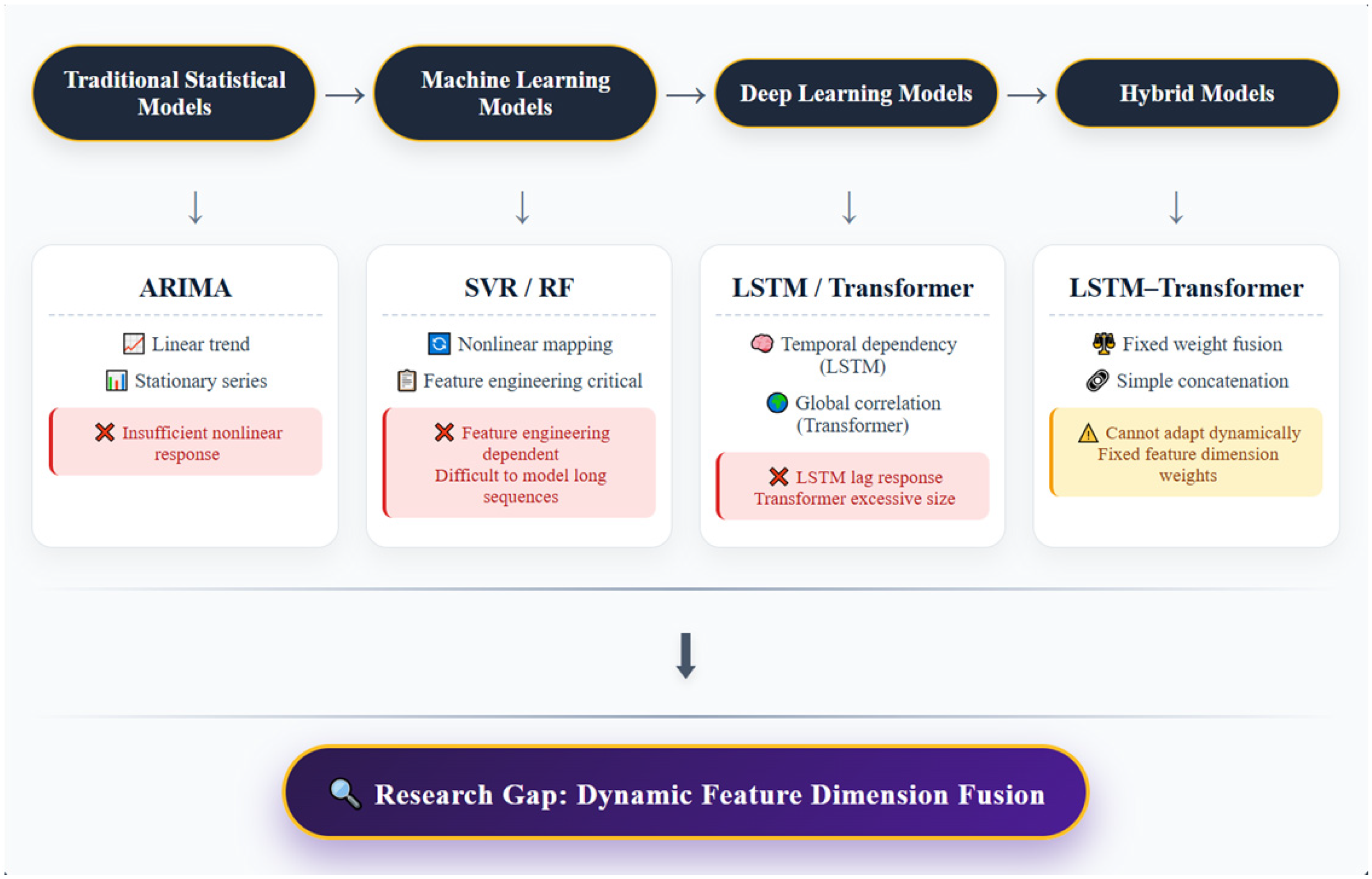
Time-series forecasting forms the foundation of microgrid energy management, with forecasting accuracy directly influencing the effectiveness of scheduling strategy optimization. Figure 2 illustrates the evolution of time-series forecasting techniques and identifies the research gap addressed in this work.

Traditional methods such as ARIMA can depict linear trends. However, they fail to capture nonlinear patterns caused by sudden weather changes or load surges, resulting in large prediction errors under the strongly non-stationary conditions of rural microgrids [17].

LSTM networks employ gating mechanisms to capture long-term temporal dependencies [6], and have been widely applied in load forecasting. However, their recursive structure limits their ability to capture global dependencies, leading to delayed responses to sudden weather events. Although LSTM can effectively extract temporal evolution patterns, its sequential nature limits sensitivity to abrupt changes far in the past. When facing minute-level fluctuations in PV output under cloudy conditions, delayed responses often occur.

Transformer models achieve global dependency modeling through self-attention mechanisms [5], enabling rapid responses to non-stationary events such as sudden weather changes. Nevertheless, standard Transformers typically have over 10M parameters, far exceeding the memory budgets of edge devices. Furthermore, their substantial parameter count and high computational cost make direct deployment on Raspberry Pi 4B-class embedded devices impractical, and overfitting frequently occurs with small-sample data.

To combine the advantages of both approaches, researchers have proposed LSTM–Transformer hybrid models [7]. However, existing fusion methods employ fixed weights or simple concatenation, making them unable to adapt to the dynamic fluctuation characteristics of rural microgrids. During stable periods, LSTM’s memory of cyclical patterns should be emphasized, while during abrupt events, Transformer’s global awareness becomes critical. Achieving fine-grained adaptive fusion of these two characteristics—enabling dynamic weight adjustment based on input data—represents the key to improving forecasting performance.

For edge deployment requirements, model lightweight technologies such as channel pruning and knowledge distillation have been extensively applied in the image domain; however, pruning strategies specifically designed for time-series forecasting models remain underdeveloped. Most existing methods apply global thresholds without considering the varying contributions of different layers to time-series modeling. Direct application to LSTM or Transformer architectures may result in the loss of critical temporal information. Therefore, designing a forecasting model that captures long-term temporal dependencies while rapidly responding to abrupt changes—with moderate parameter counts—constitutes the primary challenge for rural microgrid energy management.

Forecasting errors propagate to scheduling decisions. To avoid suboptimal dispatch under high uncertainty, we argue that forecasting and scheduling should be co-optimized rather than treated separately. The following section analyzes existing scheduling methods before we present our co-optimization framework.

2.3. Optimal Scheduling Methods for Microgrids

Microgrid scheduling is essentially a multi-objective, multi-constraint, nonlinear combinatorial optimization problem. Existing research methods fall into three categories: mathematical optimization, heuristic algorithms, and quantum-inspired optimization. Figure 3 provides a taxonomy of existing scheduling approaches and highlights their respective limitations.

Mathematical optimization methods, such as mixed integer linear programming (MILP) [9] and quadratic programming, can find exact optimal solutions in small-scale systems. However, as variable dimensionality increases, solution complexity grows exponentially [2]. For scheduling problems with 24 h horizons and 15 min resolution, decision variables can reach hundreds of dimensions, including 0–1 integer variables. Traditional mathematical optimization methods are inadequate for solving such problems within second-level response time constraints under the limited computing power of rural edge nodes.

Heuristic algorithms such as genetic algorithms and particle swarm optimization (PSO) balance solution quality and computational efficiency [1]. However, standard heuristic algorithms tend to fall into local optima, with convergence speed decreasing significantly as problem size increases. Distributed control strategies achieve coordination through limited communication between neighboring units, improving system reliability [18,19,20]. Although heuristic algorithms can provide feasible solutions, their global search capability is limited, making it difficult to approach optimal operating points when PV and load fluctuate drastically.

Quantum-inspired optimization algorithms draw upon superposition state concepts from quantum computing, encoding decision variables with qubits and updating probability amplitudes through quantum rotation gates to achieve efficient global search [1]. However, standard algorithms employ fixed rotation angles, which exhibit limitations in dynamic rural scenarios: excessively large rotation angles lead to slow convergence, while excessively small angles risk entrapment in local optima. Fixed rotation angles cannot adapt to dynamic changes in forecasting uncertainty. When forecasting confidence is high, local exploitation should be emphasized; when forecasting fluctuations are large, the search scope should be expanded. Without such dynamic adjustment, standard quantum-inspired algorithms fail to adapt to rural microgrids’ fluctuating conditions, leading to suboptimal scheduling decisions.

Given the abundant water resources in rural areas, microgrid dispatching strategies incorporating small pumped storage power stations can further improve system economy and renewable energy accommodation capacity [21]. Furthermore, most existing research treats forecasting and scheduling separately, failing to fully utilize forecasting uncertainty information to guide the search process. Therefore, designing a scheduling algorithm that integrates forecasting confidence and dynamically balances exploration and exploitation is central to achieving forecasting–scheduling co-optimization.

2.4. Edge-Side Model Lightweight Technologies

Edge-side resources are constrained, requiring lightweight processing of deep learning models before deployment [16]. Mainstream techniques include channel pruning, knowledge distillation, and quantization. However, most existing lightweight technologies target image classification tasks, with pruning strategies for time-series forecasting models remaining insufficiently developed [10].

Channel pruning reduces parameter counts without altering network structure by eliminating convolution kernels or neurons with low contribution. However, traditional pruning methods predominantly employ global unified thresholds, without considering the differing contributions of layers to time-series modeling. Shallow feature extraction layers capture local fluctuations, while deep aggregation layers model global cycles. Significant differences exist in layer importance within time-series forecasting models, necessitating differentiated pruning strategies.

Knowledge distillation employs large-scale teacher models to guide the training of small-scale student models, transferring generalization capability through soft labels. Distilled models can substantially reduce parameter counts while maintaining accuracy. However, pure distillation may not fully preserve the teacher model’s sensitive response to time-series mutation points, necessitating combination with time-series-aware loss functions.

Sensitivity analysis quantifies the influence of different layers on final results by calculating the gradient norms of each layer’s output with respect to the loss function, providing a basis for differentiated compression [13]. Higher sensitivity indicates greater layer importance, warranting preservation of more channels during pruning. However, whether gradient sensitivity fully equates to “temporal importance” in time-series forecasting requires verification, with specialized sensitivity indicators needed—tailored to time-series characteristics.

Therefore, designing a lightweight strategy tailored to the structural characteristics of time-series models—while maintaining forecasting accuracy—represents the final barrier to edge deployment.

2.5. Research Gaps and Positioning of This Paper

In summary, three critical gaps exist in existing rural microgrid energy management research:

(1)

The gap between forecasting accuracy and lightweight deployment: High-precision fusion models such as K-NBEATSx cannot be deployed at the edge [7], while lightweight models suffer sharply increased errors under fluctuating conditions.

(2)

The gap between global optimization and real-time response: Although intelligent algorithms such as bilevel optimization can approach optimal solutions, their excessive computation time makes meeting second-level scheduling requirements difficult [22].

(3)

The gap between technological advancement and scenario adaptability: Most studies remain at the simulation stage without validation under real-world rural conditions [14].

Table 1. Research gaps and corresponding contributions.

S	Research Gap	Contribution
Time-series forecasting	LSTM global dependency limited; excessive Transformer parameter count; hybrid models use fixed weights	AGDN with gated fusion for dynamic weight allocation
Optimized scheduling	Standard quantum-inspired algorithms use fixed rotation angles	PUG-QIO with adaptive rotation angles guided by prediction confidence
Edge deployment	Unified pruning thresholds ignore layer-wise differences	TSADP with temporal sensitivity-guided differentiated pruning
Scenario validation	Most studies stop at simulation	30-day field trial validation

summarizes the research gaps addressed by this paper.

To address these gaps, this paper proposes an energy management system with forecasting–scheduling co-optimization and edge deployability. The core innovations include the following:

(1)

Adaptive Gated Dual-stream Network (AGDN): Achieves fine-grained fusion of LSTM and Transformer through a feature-dimensional gated fusion mechanism.

(2)

Prediction Uncertainty-Guided Quantum-Inspired Optimization (PUG-QIO): Maps prediction confidence intervals to adaptive rotation angles, enabling dynamic exploration–exploitation trade-offs.

(3)

Temporal Sensitivity-Aware Differentiated Pruning (TSADP): Maintains forecasting accuracy at 63% compression ratio through layer-wise pruning based on temporal contribution.

3. System Requirements Analysis

3.1. System Function and Performance Requirements

The rural microgrid energy management system provides four core functions: data sensing, time-series forecasting, optimal scheduling, and human–computer interaction [2]. The system adopts a “local autonomy first, cloud collaboration supplement” hierarchical control architecture [1].

Table 2. System performance requirements.

Metric Dimension	Indicator Name	Target Value	Test Conditions
Forecasting accuracy	MAPE for load forecasting	≤4.5%	24 h forecast window, 5 min sampling interval
Forecasting accuracy	PV forecast nRMSE	≤10%	24 h forecast window, stratified by weather type
Real-time response	End-to-end processing latency	≤10 s	From data acquisition completion to dispatch instruction generation
System reliability	Average annual system availability	≥95%	Including planned maintenance and unplanned failures
Weak communication availability	Core function availability at packet loss rate ≤ 20%	≥90%	Based on 48 h of continuous testing

presents the key performance indicators and their test conditions.

Data sensing: Real-time acquisition of photovoltaic array output, energy storage system states (SOC and SOH), multi-type load power, and meteorological parameters (irradiance, temperature, humidity, wind speed). Supports multi-protocol heterogeneous device access including Modbus RTU/TCP, IEC 104, and MQTT, with breakpoint resumption capability.

Time-series forecasting: Based on historical data and meteorological information, forecasts load and PV output curves for the next 24–96 h, outputting point predictions with confidence intervals as input to the scheduling module.

Optimal scheduling: Based on forecast results, the system generates energy storage charging/discharging strategies, diesel generator start/stop schedules, and power purchase/sale schemes, comprehensively considering time-of-use pricing, equipment operational constraints, and energy storage lifetime.

Human–computer interaction: The system provides local HMI and remote Web-based visual monitoring interfaces, supporting mobile terminal access for real-time viewing of operational status, alarm information, and scheduling strategies.

3.2. Rural Environment Adaptation Requirements

The rural operating environment imposes additional requirements on the system, which must satisfy the following adaptation criteria while maintaining core functionality.

Low-computing-power edge deployment: The system must operate stably on Raspberry Pi 4B-class embedded devices, with idle-state memory occupancy below 500 MB and average CPU utilization below 60% [16].

Adaptation to weak communication environments: Support for 4G/LoRa hybrid networking with multi-link intelligent switching [1]. Upon complete communication interruption, the system must switch to local autonomous mode to maintain basic scheduling capability for ≥72 h [11,13].

Offline fault tolerance and data consistency: A ring-buffer local cache database is established with cache capacity for ≥7 days of operational data. After communication restoration, the system must implement breakpoint resumption and conflict resolution mechanisms to ensure a data integrity rate ≥ 99.5% [11,12].

Unattended operation and environmental adaptability: The system must possess automatic fault diagnosis and recovery mechanisms, achieving automatic identification and recovery of over 90% of faults. Edge node hardware must satisfy industrial protection requirements, with an operating temperature range from −20 °C to 60 °C and protection level ≥ IP54, suitable for rural power grid voltage fluctuation scenarios [13].

4. System Design

4.1. System Architecture Design

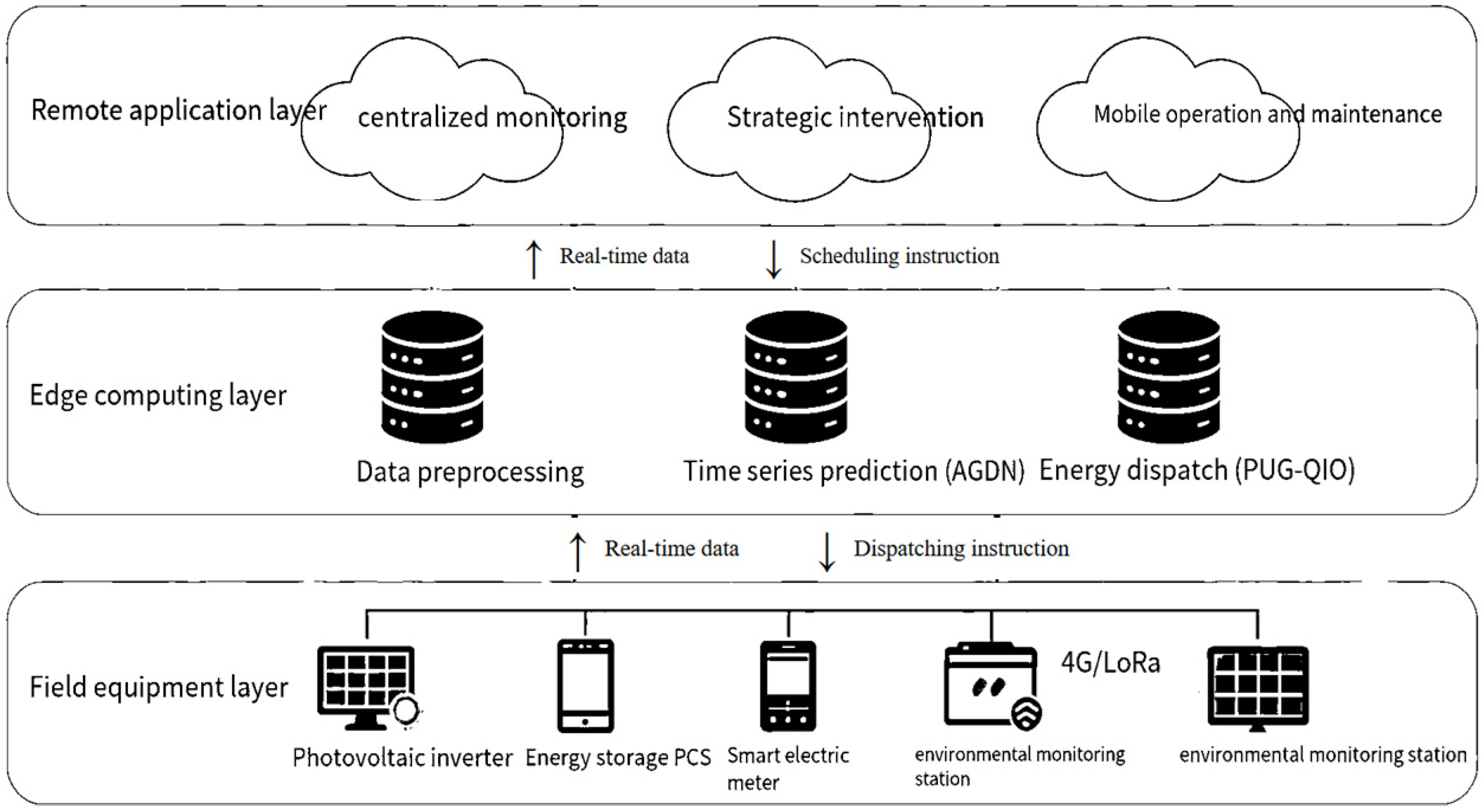
To address the triple critical constraints of severe physical-layer fluctuations, weak information-layer communication, and limited computing-layer resources in rural microgrid environments, this paper designs a hierarchical energy management system with forecasting–scheduling co-optimization and edge deployability. The system architecture, illustrated in Figure 4, comprises three layers from bottom to top.

Field equipment layer: Deployed on the primary equipment side of the microgrid, this layer includes photovoltaic inverters, Power Conversion Systems (PCS), smart meters, environmental monitoring stations, and various sensors. This layer performs two primary functions:

(1)

Data acquisition: Through multi-protocol hybrid access including Modbus RTU (RS-485 bus), IEC 104 (Ethernet), and CAN (energy storage internal bus), 38 types of operating parameters are collected at 5 s sampling intervals. These parameters include PV DC power, energy storage SOC/SOH, three-phase load power, and irradiance.

(2)

Command execution: The layer receives scheduling instructions from the edge computing layer to control energy storage charging/discharging power, diesel generator start/stop operations, and grid-connected switch states. A local cache provides short-term data buffering (≥2 h) during communication exceptions.

Edge computing layer: The Raspberry Pi 4B edge node deployed in the rural power distribution room serves as the decision-making core. This layer contains three functional modules with the following data flow paths:

(1)

Path 1—Data acquisition and preprocessing (continuous operation, triggered every 5 s): Raw data undergoes temporal alignment, anomaly detection, imputation, and standardization before being written to a local time-series database. Average processing time: 320 ms.

(2)

Path 2—Time-series forecasting (triggered every 15 min by the scheduling module, or automatically when new data accumulation exceeds 1 h): The forecasting module reads 72 h of historical data, executes the Adaptive Gated Dual-stream Network (AGDN), and outputs load and PV predictions with 95% confidence intervals for the next 24 h. Single inference time: approximately 31 ms (after lightweight deployment).

(3)

Path 3—Energy scheduling (rolling optimization every 15 min, or triggered when deviation between predicted and actual values exceeds threshold): The scheduling module takes the latest prediction results and real-time status as input, runs the Prediction Uncertainty-Guided Quantum-Inspired Optimization (PUG-QIO) algorithm, and generates energy storage charging/discharging plans, diesel generator start/stop schedules, and power purchase/sale strategies for the next 24 h (96 time slots). Average solution time: 5.3 s. Generated scheduling instructions are transmitted to the field equipment layer through the communication link.

(4)

Path 4—Local autonomy and mode switching (communication link quality detected every second): When communication is interrupted, the system automatically switches to degraded or emergency mode to maintain basic scheduling capability (see Section 4.4.3).

Remote application layer: Deployed on cloud servers at the township monitoring center, this layer provides centralized monitoring, policy intervention, and mobile operation and maintenance services. In normal mode, edge nodes upload operational data and scheduling results every 15 min and receive cloud configuration adjustments. After communication restoration, local cache data is automatically synchronized.

This three-layer structure and its data flow relationships establish the architectural foundation for subsequent detailed design, encompassing the complete process from data acquisition through edge decision making to cloud monitoring.

4.2. Design of Data Acquisition Module

The data acquisition module achieves reliable acquisition and high-fidelity preprocessing of multi-source operational data under constraints of heterogeneous equipment (multi-manufacturer, multi-protocol) and fragile communication (4G/LoRa hybrid networking).

4.2.1. Acquisition Objects and Sampling Strategy

The collection objects cover four categories of heterogeneous data sources. A variable sampling rate adaptive acquisition strategy is employed, as detailed in

Table 3. Multi-source data acquisition parameters and variable sampling rate strategy.

Data Category	Objects to Collect	Interface Protocol	Steady-State Sampling Interval	Wave-Dynamic Trigger Conditions	Wave-Dynamic Sampling Interval
Generation unit	PV inverter (DC power, voltage, current)	Modbus RTU (RS-485)	5 s	Power change rate > 10%/min	1 s
Energy storage system	SOC, SOH, charge/discharge power, cell voltage/temperature	CAN 2.0B	5 s	Charge/discharge state switch	1 s
Load side	Total incoming line power, branch loop power (cold chain/irrigation)	Modbus TCP (Ethernet)	5 s	Load surge > 15%/min	1 s
Weather station	Irradiance, ambient temperature, humidity, wind speed	LoRa (gateway convergence)	1 min	Irradiance change > 200 W/m2·min	10 s

.

The variable sampling rate adaptive acquisition strategy ensures complete recording of key fluctuation events (such as sudden PV power changes and load surges) while controlling average daily data volume within 3.5 GB. This prevents storage overflow on embedded devices while balancing data fidelity and storage efficiency.

4.2.2. Communication Architecture Design

A 4G-primary + LoRa-backup dual-link redundant communication architecture is adopted:

(1)

Primary link (4G): Through DTU transparent transmission, supporting TCP/MQTT protocols, used for real-time data transmission and cloud command reception.

(2)

Standby link (LoRa): Ad-hoc network mode covering scattered nodes (weather stations, irrigation loads) within a 5 km radius, used for critical data backhaul during communication interruptions.

The link quality dynamic evaluation index is defined as the following:

$$Q_{\mathrm{link}}=\alpha {\tilde{R}}_{ss}+\beta \left(1-P_{\mathrm{loss}}\right)+\gamma \left(1−{\displaystyle \frac{L_{\mathrm{delay}}}{L_{\max }}}\right)$$

(1)

where ${\tilde{R}}_{ss}\in [0,1]$ is the normalized signal strength (linearly mapped from −120 dBm to 0 and −50 dBm to 1); $P_{\mathrm{loss}}\in [0,1]$ is the average packet loss rate over a 30 s sliding window; $L_{\mathrm{delay}}$ is the measured average transmission delay (seconds); and $L_{\max }=10$ s is the maximum tolerable delay threshold. The coefficients satisfy $\alpha +\beta +\gamma =1$, with values $\alpha =0.5, \beta =0.3,\gamma =0.2$ selected to prioritize signal stability while accounting for latency and packet loss.

When $Q_{\mathrm{link}}<0.6$ persists for more than 30 s, the system automatically switches communication links. The switching process remains transparent to upper-layer applications.

4.2.3. Data Preprocessing Pipeline

Three levels of preprocessing are performed locally at edge nodes to ensure data quality meets prediction model input requirements:

Level 1: Temporal alignment

Based on NTP server time, timestamps from all heterogeneous data sources are linearly interpolated and aligned to 5 s equal-interval time series. Alignment error is controlled within ±100 ms.

Level 2: Anomaly detection and correction

Two anomaly detection methods are employed jointly:

(1)

Statistical method: Based on the 3σ principle, data points beyond mean ±3 standard deviation are identified.

(2)

Physical method: Based on rate-of-change constraints, power change rates exceeding 50%/s (amplitude change exceeding 50% of rated power per second) are flagged as abnormal. This threshold is determined from physical response characteristics of PV and load.

Abnormal points are corrected using cubic spline interpolation. If more than 10 consecutive abnormal points occur, the entire segment is marked as missing.

Level 3: Missing value imputation

A hierarchical imputation strategy is used:

(1)

Short gaps (≤30 s): Forward fill (retain last valid value).

(2)

Moderate gaps (30 s to 5 min): Predictive imputation using ARIMA (2, 1, 2) model, where 2 is the autoregressive order, 1 is the differencing order, and 2 is the moving average order. Model parameters are optimized on historical datasets using Bayesian Information Criterion and updated online based on historical contemporaneous data.

(3)

Long gaps (>5 min): Marked as unavailable, triggering robust mode switching in the scheduling module.

After preprocessing, data are normalized using the Z-Score method:

$$\widehat{x}={\displaystyle \frac{x-u}{\sigma }}$$

(2)

where $u$ and $\sigma$ are the mean and standard deviation of the feature on the training set. Standardized data are written to the local time-series database (SQLite). The preprocessing pipeline averages 320 ms on Raspberry Pi 4B, meeting the real-time requirement of the 5 s sampling period.

4.3. Time-Series Forecasting Subsystem: Adaptive Gated Dual-Stream Network (AGDN)

Given the multi-scale fluctuation characteristics of rural microgrid load and PV output—agricultural cycles superimposed with minute-level random fluctuations, abrupt changes during sunny days, and continuous downturns during rainy days—a single model struggles to capture both temporal dependencies and global correlations simultaneously. This paper proposes the Adaptive Gated Dual-stream Network (AGDN), which employs LSTM and Transformer dual encoders to extract sequence-dependent features and global associations, respectively, with a gated fusion mechanism introduced to achieve dynamic weight allocation at the feature-dimension level.

4.3.1. Problem Formulation

Let the historical input window length be $L=72$ h, feature dimension $d=8$ (including load, photovoltaic power, irradiance, temperature, humidity, wind speed, time, and day type), and sampling interval $\mathsf{\Delta }t=5$ min. The input sequence is $\mathrm{X}=\{x_1,x_2, \dots ,x_{\mathrm{T}}\}\in {\mathbb{R}}^{\mathrm{T}\times \mathrm{d}}$, where $\mathrm{T}=\mathrm{L}/\mathsf{\Delta }\mathrm{t}=864$ is the number of time steps. The model outputs the forecast sequence for future $H=24$ h: $\mathrm{Ŷ}=\{{\mathrm{ŷ}}_{(\mathrm{t}+1)},{\mathrm{ŷ}}_{(\mathrm{t}+2)},\dots ,{\mathrm{ŷ}}_{\mathrm{H}}\}\in {\mathbb{R}}^{\mathrm{H}}$.

The forecasting task is formalized as learning a mapping function $f:{\mathbb{R}}^{\mathrm{T}\times \mathrm{d}}\to {\mathbb{R}}^{\mathrm{H}}$ to minimize prediction error:

$$\mathrm{m}\mathrm{i}\mathrm{n}\parallel Y-\widehat{Y}\parallel$$

where $\mathrm{Y}\in {\mathbb{R}}^{\mathrm{H}}$ is the true value sequence for $\mathrm{H}$ hours in the future, and $\Vert ·\Vert$ denotes a norm (mean squared error is used in this paper; see Section 4.3.6).

4.3.2. Model Overall Architecture

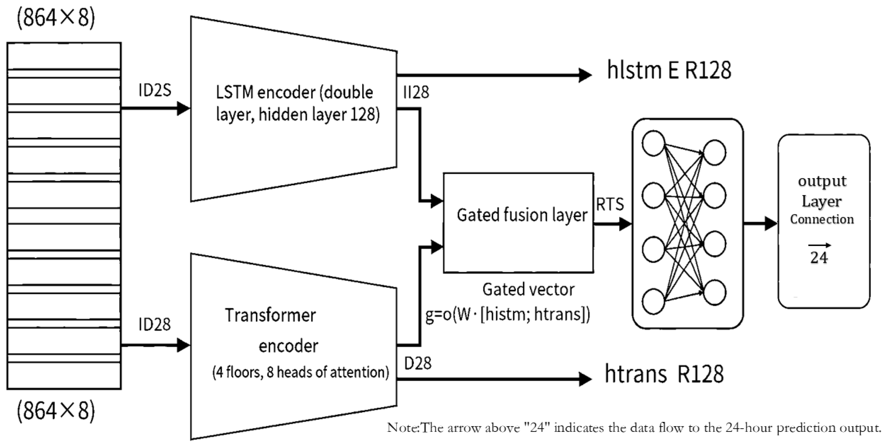
The overall architecture of AGDN, illustrated in Figure 5, consists of four components:

(1)

LSTM encoding branch: Extracts long and short-term temporal dependence features, outputting feature vector ${\mathbf{h}}_{\mathrm{lstm}}$.

(2)

Transformer encoding branch: Captures global correlation characteristics, outputting feature vector ${\mathbf{h}}_{\mathrm{trans}}$.

(3)

Gated fusion layer: Dynamically fuses features from both branches to generate fusion feature vector ${\mathbf{h}}_{\mathrm{fusion}}$.

(4)

Output layer: Maps fused features to final prediction result $\mathrm{Ŷ}$.

The data flow proceeds as follows: input sequence $\mathrm{X}$ enters two parallel branches; after feature extraction, both branch outputs are fed into the gated fusion layer; the merged features are then mapped to prediction results through the output layer.

4.3.3. LSTM Encoding Branch

A two-layer stacked Long Short-Term Memory (LSTM) network extracts temporal dependence features. LSTM addresses long-sequence gradient vanishing through gating mechanisms. The core computation unit is as follows:

$$\begin{array}{cc}{\mathbf{f}}_t& =\sigma \left({\mathbf{W}}_f\left[{\mathbf{h}}_{t-1},{\mathbf{x}}_t\right]+{\mathbf{b}}_f\right)\\ {\mathbf{i}}_t& =\sigma \left({\mathbf{W}}_i\left[{\mathbf{h}}_{t-1},{\mathbf{x}}_t\right]+{\mathbf{b}}_i\right)\\ {\mathbf{o}}_t& =\sigma \left({\mathbf{W}}_o\left[{\mathbf{h}}_{t-1},{\mathbf{x}}_t\right]+{\mathbf{b}}_o\right)\\ {\mathbf{c}}_t& ={\mathbf{f}}_t\odot {\mathbf{c}}_{t-1}+{\mathbf{i}}_t\odot \tanh \left({\mathbf{W}}_c\left[{\mathbf{h}}_{t-1},{\mathbf{x}}_t\right]+{\mathbf{b}}_c\right)\\ {\mathbf{h}}_t& ={\mathbf{o}}_t\odot \tanh \left({\mathbf{c}}_t\right)\end{array}$$

(3)

where ${\mathbf{f}}_t, {\mathbf{i}}_t,{\mathbf{o}}_t$ are the forget gate, input gate, and output gate, respectively; ${\mathbf{c}}_t$ is the cell state; ${\mathbf{h}}_t$ is the hidden state; ${\mathbf{W}}_f,{\mathbf{W}}_i,{\mathbf{W}}_o,{\mathbf{W}}_c$ are weight matrices; ${\mathbf{b}}_f,{\mathbf{b}}_i,{\mathbf{b}}_o,{\mathbf{b}}_c$ are bias terms; $\sigma (·)$ is the Sigmoid activation function with output range $(0,1)$; $\mathrm{t}\mathrm{a}\mathrm{n}\mathrm{h}(·)$ is the hyperbolic tangent activation function with output range $(-1,1)$; and $\odot$ denotes element-wise multiplication.

A two-layer LSTM was selected with hidden dimension $d_{lstm}=128$ in each layer (i.e., the hidden state at each time instant is a 128-dimensional vector). The first LSTM processes the input sequence $X$ and outputs a sequence of hidden states:

$${\mathbf{H}}^{\left(1\right)}=\{{\mathbf{h}}_1^{\left(1\right)},{\mathbf{h}}_2^{\left(1\right)},\dots ,{\mathbf{h}}_t^{\left(1\right)}\},{\mathbf{h}}_t^{\left(1\right)}\in {\mathbb{R}}^{128}$$

where superscript $\left(1\right)$ denotes the first layer and subscript $t$ denotes the time step, with total time steps $T=864$. This hidden state sequence serves as input to the second LSTM layer.

The second LSTM layer takes the hidden state sequence from the first layer as input to further extract high-level temporal features:

$${\mathbf{h}}_t^{\left(2\right)}={\mathrm{LSTM}}^{\left(2\right)}\left({\mathbf{h}}_t^{\left(1\right)},{\mathbf{h}}_{t-1}^{\left(2\right)}\right),t=\mathrm{1,2},\dots ,T$$

where ${\mathbf{h}}_t^{\left(2\right)}\in {\mathbb{R}}^{128}$ is the hidden state of the second LSTM layer at time $t$, with zero vector initialization ${\mathbf{h}}_0^{\left(2\right)}=0$.

The hidden state of the second LSTM layer at time step $t$, denoted as ${\mathbf{h}}_t^{\left(2\right)}\in {\mathbb{R}}^{128}$, can be explicitly written as

$${\mathbf{h}}_t^{\left(2\right)}={[{\mathbf{h}}_{\{t,1\}}^{\left(2\right)},{\mathbf{h}}_{\{t,2\}}^{\left(2\right)},\dots ,{\mathbf{h}}_{\{t,128\}}^{\left(2\right)}]}^{\mathrm{T}}$$

The initial hidden state is set to the zero vector: ${\mathbf{h}}_0^{\left(2\right)}=\mathsf{0}={[\mathsf{0},\mathsf{0},\dots ,\mathsf{0}]}^{\mathrm{T}}$ (128 zeros).

After recursive calculation over $T=864$ time steps, the last hidden state is taken as the LSTM branch extracted temporal feature vector:

$${\mathbf{h}}_{\mathrm{lstm}}={\mathbf{h}}_T^{\left(2\right)}\in {\mathbb{R}}^{128}$$

This feature vector encodes periodic patterns, trend changes, and short-term fluctuation information of load and PV over the 72-h history. The two-layer structure captures more complex temporal dependencies than single-layer LSTM, with hidden dimension 128 balancing representational capacity and computational cost. The LSTM branch contains approximately 140,000 parameters, accounting for 40.8% of AGDN total parameters.

4.3.4. Transformer Encoding Branch

Transformer employs self-attention mechanisms to establish global dependencies in one step, enabling sharp response to non-stationary events such as sudden weather changes. This paper adopts the standard Transformer encoder structure, comprising the following components:

Positional encoding: Since Transformer lacks recurrent structure, positional information is preserved through positional encoding. Sinusoidal positional encoding is used:

$$\begin{array}{cc}{\mathbf{P}}_{\left(t,2i\right)}& =\sin \left({\displaystyle \frac{t}{{10000}^{\frac{2i}{d_{\mathrm{model}}}}}}\right)\\ {\mathbf{P}}_{\left(t,2i+1\right)}& =\cos \left({\displaystyle \frac{t}{{10000}^{\frac{2i}{d_{\mathrm{model}}}}}}\right)\end{array}$$

(4)

where $t=\mathrm{1,2},\dots ,T$ is the time step index; $i=\mathrm{0,1},\dots , d_{\mathit{model}}/2-1$ is the dimension index; and $d_{\mathrm{model}}=128$ is the model dimension. The positional encoding matrix $\mathit{P}\in {{\mathbb{R}}^{\mathrm{Txd}}}_{\mathrm{MODEL}}$ is added to the input embedding to obtain position-aware input:

$${\mathbf{X}}_{\mathrm{pos}}=\mathbf{X}{\mathbf{W}}_{\mathrm{embed}}+\mathbf{P}$$

where ${\mathbf{W}}_{\mathrm{embed}}\in {{\mathbb{R}}^{\mathit{d}\times \mathit{d}}}_{\mathrm{MODEL}}$ is the input embedding matrix mapping original feature dimensions ($d=8$) to model dimensions ($d_{\mathrm{model}}=128$).

Multi-head self-attention: For input sequence ${\mathbf{X}}_{\mathrm{pos}}$, query matrix $Q$, key matrix $K$, and value matrix $V$ are obtained through linear transformation:

$$\mathbf{Q}={\mathbf{X}}_{\mathrm{pos}}{\mathbf{W}}^Q,\mathbf{K}={\mathbf{X}}_{\mathrm{pos}}{\mathbf{W}}^K,\mathbf{V}={\mathbf{X}}_{\mathrm{pos}}{\mathbf{W}}^V$$

Scaled dot-product attention is computed as

$$\mathrm{Attention}\left(\mathbf{Q},\mathbf{K},\mathbf{V}\right)=\mathrm{softmax}\left({\displaystyle \frac{\mathbf{Q}{\mathbf{K}}^T}{\sqrt{d_k}}}\right)\mathbf{V}$$

(5)

where $d_k={\displaystyle \frac{d_{\mathrm{model}}}{h}}=16$ is the dimension of each attention head and $h=8$ is the number of attention heads. Multi-head attention projects feature into different representation subspaces and computes in parallel:

$$\begin{array}{cc}{\mathrm{head}}_i& =\mathrm{Attention}\left(\mathbf{Q}{\mathbf{W}}_i^Q,\mathbf{K}{\mathbf{W}}_i^K,\mathbf{V}{\mathbf{W}}_i^V\right)\\ \mathrm{MultiHead}\left(\mathbf{Q},\mathbf{K},\mathbf{V}\right)& =\mathrm{Concat}\left({\mathrm{head}}_1,\dots ,{\mathrm{head}}_h\right){\mathbf{W}}^O\end{array}$$

(6)

where ${\mathbf{W}}_i^Q,{\mathbf{W}}_i^K,{\mathbf{W}}_i^V\in {\mathbb{R}}^{d_{\mathrm{model}}\times d_k},{\mathbf{W}}^O\in {\mathbb{R}}^{d_{\mathrm{model}}\times d_{\mathrm{model}}}$ are learnable parameters.

Feedforward network: Each encoding layer is followed by two fully-connected layers introducing nonlinear transformation:

$$\mathrm{FFN}\left(\mathbf{x}\right)=\max \left(0,\mathbf{x}{\mathbf{W}}_1+{\mathbf{b}}_1\right){\mathbf{W}}_2+{\mathbf{b}}_2$$

(7)

where ${\mathbf{W}}_1\in {\mathbb{R}}^{d_{\mathrm{model}}\times d_{ff}},{\mathbf{W}}_2\in {\mathbb{R}}^{d_{ff}\times d_{\mathrm{model}}},d_{ff}=256$ is the feedforward hidden dimension, and $\mathrm{m}\mathrm{a}\mathrm{x}(0,·)$ is the ReLU activation function.

Layer normalization and residual connection: Residual connections and layer normalization are applied after each sub-layer (multi-head attention, feedforward network):

$${\mathbf{x}}_{\mathrm{out}}=\mathrm{LayerNorm}\left(\mathbf{x}+\mathrm{Sublayer}\left(\mathbf{x}\right)\right)$$

(8)

A stack of 4-layer Transformer encoders was selected, with each layer having dimension $d_{\mathrm{model}}=128$. After four encoding layers, the output sequence is averaged and pooled along the time dimension to obtain the global feature vector:

$${\mathbf{h}}_{\mathrm{trans}}={\displaystyle \frac{1}{T}}{\sum }_{t=1}^T{\mathbf{z}}_t\in {\mathbb{R}}^{128}$$

where ${\mathbf{z}}_t\in {\mathbb{R}}^{128}$ is the output of the last encoder layer at time $t$. This feature vector captures global dependencies across the entire history window and maintains keen responsiveness to non-stationary events such as sudden weather changes and load surges.

The Transformer encoding branch contains approximately 170,000 parameters, accounting for 49.6% of AGDN total parameters.

4.3.5. Gated Fusion Mechanism

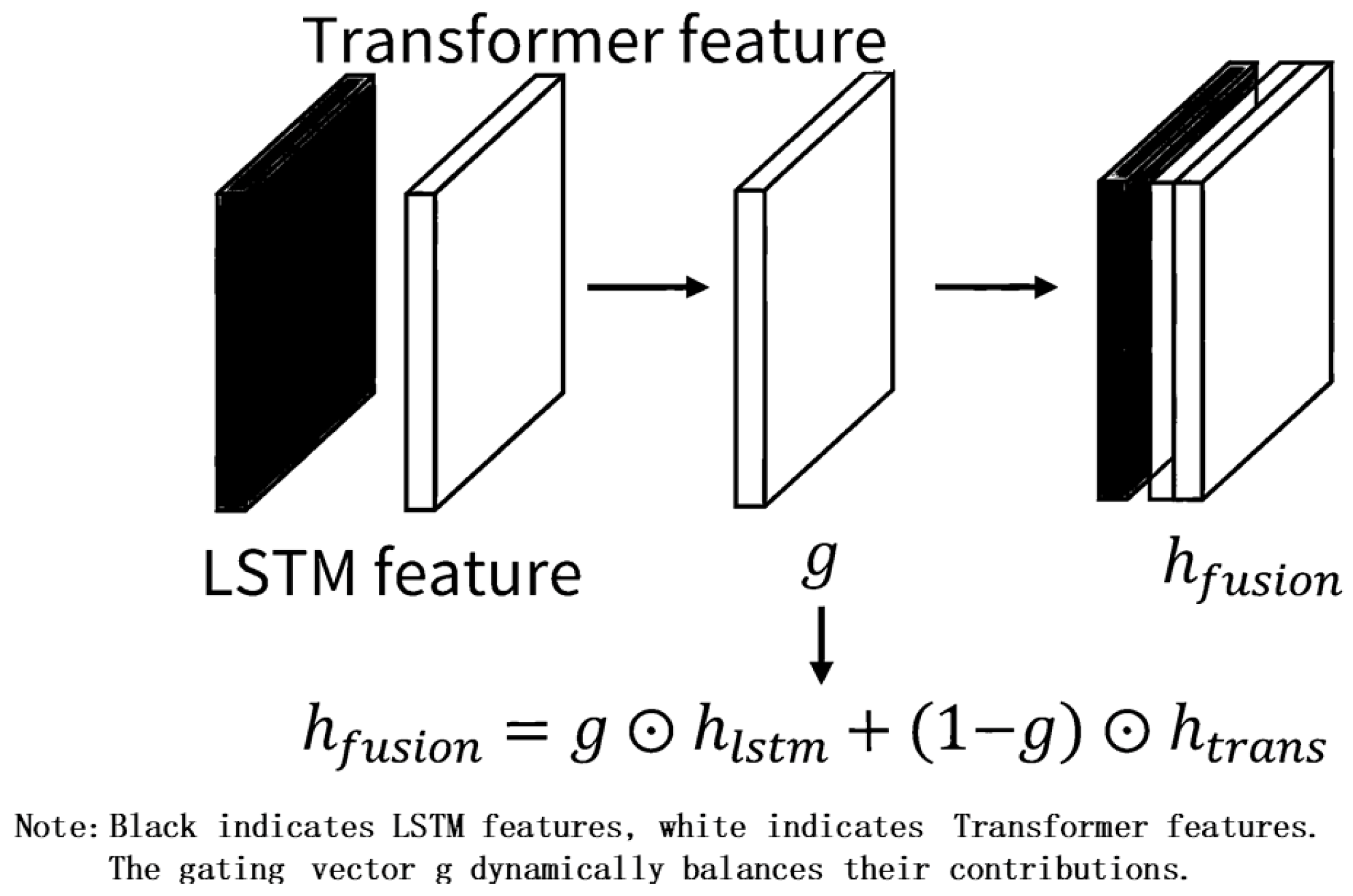
The contributions of the two branches vary dynamically with scenarios: stationary periods (continuous sunny days) rely more on LSTM’s periodic memory, while abrupt moments (sudden rainfall) require Transformer’s global perception. This paper designs a gated fusion mechanism at the feature-dimension level to achieve fine-grained adaptive fusion, as illustrated in Figure 6.

The temporal characteristics of rural microgrids can be decomposed into two types: stationary periodic components (daily load patterns, seasonal PV output) and non-stationary abrupt components (sudden output drops, load surges). LSTM excels at capturing periodic patterns through its recursive structure, while Transformer responds sharply to abrupt events via self-attention. However, these components are often superimposed in feature space, making explicit separation difficult at the input layer. The gated fusion mechanism learns a “soft selector” at the feature-dimension level: when a dimension’s gating value approaches 1, it primarily inherits LSTM output (focusing on stationary components); when the value approaches 0, it primarily inherits Transformer output (focusing on abrupt components). This enables the model to dynamically assign fusion weights to different feature dimensions according to input characteristics.

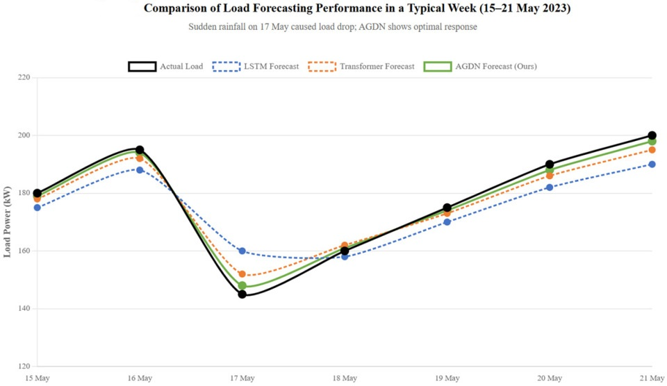
Visual validation: To test this hypothesis, a typical abrupt scenario from the test set was selected (sudden rainfall on 17 May 2023, causing brief load drop, as shown in Figure 5). Gating vector $\mathbf{g}\in {\mathbb{R}}^{128}$ analysis reveals that approximately 37% of dimensions have gating values less than 0.3 (biased toward Transformer), corresponding mainly to feature dimensions related to abrupt changes (e.g., irradiance change rate, high-frequency load fluctuations). Approximately 41% of dimensions have gating values greater than 0.7 (biased toward LSTM), corresponding mainly to cycle-related feature dimensions (e.g., time, day type, smoothed load trends). Remaining dimensions occupy intermediate states, reflecting synergistic contributions from both branches. This distribution aligns with the theoretical hypothesis, confirming that the gating mechanism achieves dynamic routing of feature dimensions.

Feature alignment and weighted fusion: To ensure feasibility of element-wise multiplication, features from both branches are projected to the same dimension:

$${\tilde{\mathbf{h}}}_{\mathrm{lstm}}={\mathbf{W}}_{\mathrm{lstm}}{\mathbf{h}}_{\mathrm{lstm}}+{\mathbf{b}}_{\mathrm{lstm}}\in {\mathbb{R}}^{128}$$

$${\tilde{\mathbf{h}}}_{\mathrm{trans}}={\mathbf{W}}_{\mathrm{trans}}{\mathbf{h}}_{\mathrm{trans}}+{\mathbf{b}}_{\mathrm{trans}}\in {\mathbb{R}}^{128}$$

where ${\mathbf{W}}_{\mathrm{lstm}},{\mathbf{W}}_{\mathrm{trans}}\in {\mathbb{R}}^{128\times 128}$ are projection matrices.

The final fusion feature is the dimension-wise weighted sum of both branch outputs:

$${\mathbf{h}}_{\mathrm{fusion}}=\mathbf{g}\odot {\tilde{\mathbf{h}}}_{\mathrm{lstm}}+(\mathbf{1}-\mathbf{g})\odot {\tilde{\mathbf{h}}}_{\mathrm{trans}}\in {\mathbb{R}}^{128}$$

where $\odot$ represents element-wise multiplication and $\mathbf{1}$ is an all-ones vector. This mechanism enables the model to autonomously learn the decision boundary of “when to trust LSTM and when to trust Transformer” during training.

Compared with scalar weighting, gated fusion achieves improvements at three levels: feature-dimension differentiation, temporal dynamic adaptation, and fine-grained control. Experimental results (Section 5.4.1) show that gated fusion improves load forecasting by 0.6 percentage points compared with scalar weighting, verifying mechanism effectiveness.

4.3.6. Output Layer and Loss Function

Fused features are mapped to prediction output through a two-layer fully-connected network:

$$\widehat{Y}={\mathbf{W}}_2\cdot \phi ({\mathbf{W}}_1{\mathbf{h}}_{\mathrm{fusion}}+{\mathbf{b}}_1)+{\mathbf{b}}_2\in {\mathbb{R}}^H$$

where ${\mathbf{h}}_{\mathrm{fusion}}\in {\mathbb{R}}^{128}$ is the fusion feature vector; ${\mathbf{W}}_1\in {\mathbb{R}}^{64\times 128},{\mathbf{b}}_1\in {\mathbb{R}}^{64}$ are first-layer parameters; ${\mathbf{W}}_2\in {\mathbb{R}}^{H\times 128},{\mathbf{b}}_2\in {\mathbb{R}}^H$ are second-layer parameters; $\phi (·)=max(0,·)$ is the ReLU activation function; and $H=24$ is the prediction horizon.

The training objective function is the weighted sum of mean squared error (MSE) and L2 regularization term:

$$\mathcal{L}={\displaystyle \frac{1}{N}}{\sum }_{i=1}^N\parallel {\mathbf{y}}_i-{\widehat{\mathbf{y}}}_i{\parallel }_2^2+\lambda \parallel \mathsf{\Theta }{\parallel }_2^2$$

(9)

where $N$ is batch size; ${\mathbf{y}}_i\in {\mathbb{R}}^H$ is the true value of sample $i$; ${\widehat{\mathbf{y}}}_i\in {\mathbb{R}}^H$ is the predicted value of sample $i$; $\parallel ·{\parallel }_2$ is the L2 norm; $\mathsf{\Theta }$ represents all trainable parameters; and $\lambda ={10}^{-4}$ is the regularization coefficient preventing overfitting.

The Adam optimizer was employed with initial learning rate ${10}^{-3}$ and batch size 32. An early stopping strategy was adopted: training terminated when validation set loss did not decrease for 5 consecutive epochs, and model parameters with the lowest validation loss were saved. The model was trained on an NVIDIA RTX 3090 GPU (manufactured by NVIDIA Corporation, Santa Clara, CA, USA) for approximately 2 h to convergence.

After prediction completion, output requires de-normalization to restore actual physical dimensions:

$${\widehat{y}}_{\mathrm{actual}}=\widehat{y}\cdot \sigma +\mu$$

where $\sigma ,\mu$ are the standard deviation and mean of the feature on the training set (see Section 4.2.3).

4.4. Design of Energy Scheduling Decision Module

Based on prediction results, the scheduling module optimizes energy storage charging/discharging strategies, diesel generator start/stop plans, and power purchase/sale schemes under power balance and equipment constraints, achieving collaborative optimization of operational economy and power supply reliability.

4.4.1. Multi-Objective Optimization Model

Scheduling cycle $T=24$ h, time resolution $\mathsf{\Delta }t=15$ min, total decision time slots $96$ ($24$ times $\times 4$ slots/h). Decision variables include energy storage charging power $P_t^{\mathrm{ch}}$, energy storage discharging power $P_t^{\mathrm{dis}}$, diesel generator output $P_t^{\mathrm{dg}}$, power purchase from grid $P_t^{\mathrm{buy}}$, power sale to grid $P_t^{\mathrm{sell}}$, energy storage charging state $u_t^{\mathrm{ch}}$ (0 or 1), energy storage discharging state $u_t^{\mathrm{dis}}$ (0 or 1), where $t=\mathrm{1,2},\dots ,96$.

The objective function simultaneously minimizes operating cost and maximizes power supply reliability:

$$\min {\sum }_{t=1}^T\left(c_{\mathrm{dg}}{P}_t^{\mathrm{dg}}\mathsf{\Delta }t+c_{\mathrm{buy}}{P}_t^{\mathrm{buy}}\mathsf{\Delta }t-c_{\mathrm{sell}}{P}_t^{\mathrm{sell}}\mathsf{\Delta }t+{\lambda }_{\mathrm{soc}}\mid SO{C}_t-SO{C}_{\mathrm{ref}}\mid \right)$$

(10)

where $c_{\mathrm{dg}}=1.8$ yuan/kWh is diesel generation unit cost; $c_{\mathrm{buy}}$ is time-of-use purchase price (0.8 yuan/kWh average); $c_{\mathrm{sell}}=0.4$ yuan/kWh is fixed feed-in tariff; ${\lambda }_{\mathrm{soc}}=0.5$ yuan is energy storage health penalty coefficient; $SO{C}_{\mathrm{ref}}=0.5$ is reference state of charge; and $\mathsf{\Delta }t=0.25$ h is time slot length. The four objective function terms correspond to: diesel fuel cost, power purchase cost, electricity sales revenue (negative cost), and penalty for energy storage SOC deviation from reference value.

Power balance constraint must be satisfied at each time:

$$P_t^{\mathrm{pv}}+P_t^{\mathrm{dg}}+P_t^{\mathrm{dis}}+P_t^{\mathrm{buy}}=P_t^{\mathrm{load}}+P_t^{\mathrm{ch}}+P_t^{\mathrm{sell}},\forall t$$

(11)

where $P_t^{\mathrm{pv}}$ is predicted PV output and $P_t^{\mathrm{load}}$ is predicted load. The left side represents power sources (PV + diesel + energy storage discharge + power purchase), and the right side represents power demands (electric load + energy storage charging + power sale).

Energy storage mutual exclusion constraint (cannot charge and discharge simultaneously):

$$u_t^{\mathrm{ch}}+u_t^{\mathrm{dis}}\le 1,\forall t$$

Energy storage power constraints:

$$0\le P_t^{\mathrm{ch}}\le P_{\max }{u}_t^{\mathrm{ch}},0\le P_t^{\mathrm{dis}}\le P_{\max }{u}_t^{\mathrm{dis}},\forall t$$

where $P_{\max } = 100$ kW is the maximum energy storage converter power.

Energy storage SOC recurrence relation:

$$SO{C}_{t+1}=SO{C}_t+{\displaystyle \frac{{\eta }_{\mathrm{ch}}{P}_t^{\mathrm{ch}}\mathsf{\Delta }t}{E_{\mathrm{ess}}}}-{\displaystyle \frac{P_t^{\mathrm{dis}}\mathsf{\Delta }t}{{\eta }_{\mathrm{dis}}{E}_{\mathrm{ess}}}}$$

(12)

where $SO{C}_t$ is energy storage state of charge at time $t$ (range 0–1); ${\eta }_{\mathrm{ch}},{\eta }_{\mathrm{dis}}$ are charging and discharging efficiencies; and $E_{\mathrm{ess}}=400$ kWh is rated energy storage capacity. SOC must satisfy safety boundaries:

$$SO{C}_{\min }\le SO{C}_t\le SO{C}_{\max },\forall t$$

where $SO{C}_{\mathrm{m}\mathrm{i}\mathrm{n}}=0.2$ (prevents over-discharge) and $SO{C}_{\mathrm{m}\mathrm{a}\mathrm{x}}=0.9$ (prevents overcharge).

Diesel generator output range:

$$P_{\min }\le P_t^{\mathrm{dg}}\le P_{\max },\forall t$$

where $P_{\mathrm{m}\mathrm{i}\mathrm{n}}=30$ kW (minimum stable operating power) and $P_{\mathrm{m}\mathrm{a}\mathrm{x}}=150$ kW (rated power).

Power purchase and sale constraints:

$$0\le P_t^{\mathrm{buy}}\le P_{\max },0\le P_t^{\mathrm{sell}}\le P_{\max },\forall t$$

where $P_{\mathrm{m}\mathrm{a}\mathrm{x}}=200$ kW is the grid-connected line capacity limit.

The above model constitutes a mixed-integer nonlinear programming problem with 768 decision variable dimensions (192 of which are 0–1 integer variables), which cannot be solved by traditional optimization methods within 10 s.

4.4.2. Prediction Uncertainty-Guided Quantum-Inspired Optimization (PUG-QIO)

Standard quantum-inspired optimization algorithms use fixed rotation angles to update qubit probability amplitudes, exhibiting limitations in dynamic rural scenarios. This paper proposes the Prediction Uncertainty-Guided Quantum-Inspired Optimization (PUG-QIO) algorithm. The confidence interval width from the prediction module output is embedded into the quantum search process as prior knowledge to achieve adaptive rotation angle mechanisms.

Theoretical rationale: The design rationale stems from the “exploration–exploitation” trade-off in optimization theory. During search, the algorithm must balance “exploitation” (fine-grained neighborhood search around current optimal solution) and “exploration” (expanding search scope to unknown regions). Prediction uncertainty ${\delta }_t$ reflects forecast credibility at current time: larger ${\delta }_t$ indicates stronger future PV or load volatility, lower model confidence about the future, and correspondingly reduced credibility of current optimal solution. The algorithm should focus more on “exploring” new regions to avoid local optima caused by unreliable predictions. Conversely, when ${\delta }_t$ is smaller (more accurate prediction), the algorithm should focus on “exploiting” the current optimal solution neighborhood to accelerate convergence. Therefore, mapping ${\delta }_t$ to rotation angle, with rotation angle dynamically adjusted according to uncertainty, constitutes an adaptive mechanism conforming to optimization principles.

Adaptive rotation angle calculation: Each decision variable is mapped to a qubit with state:

$$|{\psi }_i⟩={\alpha }_i|0⟩+{\beta }_i|1⟩$$

(13)

satisfying probability amplitude normalization ${\left|{\alpha }_i\right|}^2+{\left|{\beta }_i\right|}^2=1$. Qubit probability amplitude is updated via quantum rotation gate:

$$\left[\begin{array}{c}{\alpha }_i^{\prime }\\ {\beta }_i^{\prime }\end{array}\right]=\left[\begin{array}{cc}\cos \left(\Delta {\theta }_i\right)& -\sin \left(\Delta {\theta }_i\right)\\ \sin \left(\Delta {\theta }_i\right)& \cos \left(\Delta {\theta }_i\right)\end{array}\right]\left[\begin{array}{c}{\alpha }_i\\ {\beta }_i\end{array}\right]$$

(14)

The rotation angle is related to prediction uncertainty:

$$\Delta {\theta }_i=\Delta {\theta }_0\left(1+\gamma \cdot {\displaystyle \frac{{\delta }_t-{\delta }_{\mathrm{m}\mathrm{i}\mathrm{n}}}{{\delta }_{\mathrm{m}\mathrm{a}\mathrm{x}}-{\delta }_{\mathrm{m}\mathrm{i}\mathrm{n}}}}\right)$$

(15)

where $\Delta {\theta }_0=0.01\pi$ is the base rotation angle; ${\delta }_t$ is the prediction confidence interval width at time $t$; ${\delta }_{\mathrm{m}\mathrm{i}\mathrm{n}},{\delta }_{\mathrm{m}\mathrm{a}\mathrm{x}}$ are minimum and maximum confidence interval values on the training set; and $\gamma =0.5$ is the adjustment coefficient. When ${\delta }_{\mathrm{m}\mathrm{a}\mathrm{x}}={\delta }_{\mathrm{m}\mathrm{i}\mathrm{n}}$, ${\displaystyle \frac{{\delta }_t-{\delta }_{\mathrm{m}\mathrm{i}\mathrm{n}}}{{\delta }_{\mathrm{m}\mathrm{a}\mathrm{x}}-{\delta }_{\mathrm{m}\mathrm{i}\mathrm{n}}}}=0$ is defined. This mechanism automatically expands search range when prediction uncertainty is high and accelerates local convergence when uncertainty is low.

Algorithm pseudocode: To improve reproducibility, Algorithm 1 presents detailed PUG-QIO steps.

Algorithm 1 Prediction Uncertainty-Guided Quantum-Inspired Optimization (PUG-QIO)

$\mathrm{Input}: \mathrm{Prediction} \mathrm{confidence} \mathrm{interval} \mathrm{width} \mathrm{sequence} \{{\delta }_t{\}}_{t=1}^T$$, \mathrm{population} \mathrm{size} \mathrm{N}, \mathrm{maximum} \mathrm{iterations} \mathrm{M}, \mathrm{base} \mathrm{rotation} \mathrm{angle} \Delta {\theta }_0$$, \mathrm{adjustment} \mathrm{coefficient} \gamma$

$\mathrm{Output}: \mathrm{Optimal} \mathrm{scheduling} \mathrm{scheme} s^{*}$

$1: \mathrm{Initialize} \mathrm{quantum} \mathrm{population} P=\{q_1,q_2, \dots , q_N\}$$, \mathrm{where} \mathrm{each} \mathrm{individual} q_{i }={\left\{{\left({\alpha }_{ij},{\beta }_{ij}\right)}_{j=1}\right\}}^D$$, D$$\mathrm{is} \mathrm{decision} \mathrm{variable} \mathrm{dimension}, \mathrm{initial} \mathrm{probability} \mathrm{amplitudes} {\alpha }_{ij}={\beta }_{ij}=1/\sqrt{2}$

2: for iter = 1 to M do

$3: \mathrm{Observe} \mathrm{population}: \mathrm{For} \mathrm{each} \mathrm{individual} q_i$$, \mathrm{generate} \mathrm{deterministic} \mathrm{scheduling} \mathrm{scheme} s_i$$\mathrm{by} \mathrm{random} \mathrm{observation} (\mathrm{if} \mathrm{random} \mathrm{number} r < {\left|{\alpha }_{ij}\right|}^2$, bit j is 0, otherwise 1)

$4: \mathrm{Evaluate} \mathrm{fitness}: \mathrm{For} \mathrm{each} s_i$$, \mathrm{calculate} \mathrm{fitness} F={\displaystyle \frac{1}{J(s_i)+{\sum }_k{\mu }_k{\left[\max \left(0,g_k\left(s_i\right)\right)\right]}^2}}$$, \mathrm{where} J$$\mathrm{is} \mathrm{objective} \mathrm{function} \mathrm{value}, g_k$$\mathrm{is} \mathrm{constraint} k$$\mathrm{violation}, \mathrm{and} {\mu }_{\kappa }$ is penalty coefficient

$5: \mathrm{Record} \mathrm{current} \mathrm{best} \mathrm{individual} s^{*}=\arg \underset{{\mathit{s}}_{\mathit{i}}}{\max }{F}_i$

$6: \mathrm{for} \mathrm{each} \mathrm{individual} q_i$ do

7:        for each dimension j do

$8: \mathrm{Determine} \mathrm{rotation} \mathrm{direction}: \mathrm{if} \mathrm{bit} \mathrm{j} \mathrm{of} s_i$$\mathrm{is} 1, \mathrm{rotate} \mathrm{toward} |1⟩$$; \mathrm{otherwise} \mathrm{rotate} \mathrm{toward} |0⟩$

$9: \mathrm{Obtain} \mathrm{prediction} \mathrm{uncertainty} {\delta }_t$ at current time (corresponding to scheduling time slot t)

$10: \mathrm{Calculate} \mathrm{adaptive} \mathrm{rotation} \mathrm{angle}: \Delta {\theta }_{ij}=\Delta {\theta }_0\left(1+\gamma \cdot {\displaystyle \frac{{\delta }_t-{\delta }_{\mathrm{m}\mathrm{i}\mathrm{n}}}{{\delta }_{\mathrm{m}\mathrm{a}\mathrm{x}}-{\delta }_{\mathrm{m}\mathrm{i}\mathrm{n}}}}\right)$$, \mathrm{where} \mathrm{when} {\delta }_{\mathrm{m}\mathrm{a}\mathrm{x}}={\delta }_{\mathrm{m}\mathrm{i}\mathrm{n}}$$, {\displaystyle \frac{{\delta }_t-{\delta }_{\mathrm{m}\mathrm{i}\mathrm{n}}}{{\delta }_{\mathrm{m}\mathrm{a}\mathrm{x}}-{\delta }_{\mathrm{m}\mathrm{i}\mathrm{n}}}}=0$ is defined

$11: \mathrm{Update} \mathrm{probability} \mathrm{amplitude} \mathrm{with} \mathrm{quantum} \mathrm{rotation} \mathrm{gate}: \left[\begin{array}{c}{\alpha }_{ij}^{\prime }\\ {\beta }_{ij}^{\prime }\end{array}\right]=\left[\begin{array}{cc}\cos \left(\Delta {\theta }_{ij}\right)& -\sin \left(\Delta {\theta }_{ij}\right)\\ \sin \left(\Delta {\theta }_{ij}\right)& \cos \left(\Delta {\theta }_{ij}\right)\end{array}\right]\left[\begin{array}{c}{\alpha }_{ij}\\ {\beta }_{ij}\end{array}\right]$

12:        end for

13:      end for

14:      If no improvement in optimal solution for 30 consecutive generations, terminate iteration

15: end for

$16: \mathrm{return} \mathrm{Globally} \mathrm{optimal} \mathrm{scheduling} \mathrm{plan} s^{*}$

Experiments show that the proposed algorithm achieves an approximately 15% higher convergence speed than standard quantum-inspired algorithms while maintaining solution quality, with an average single-solution time of 5.3 s (measured on Raspberry Pi 4B), meeting the system response time limit of 10 s.

4.4.3. Robust Mode-Switching Mechanism

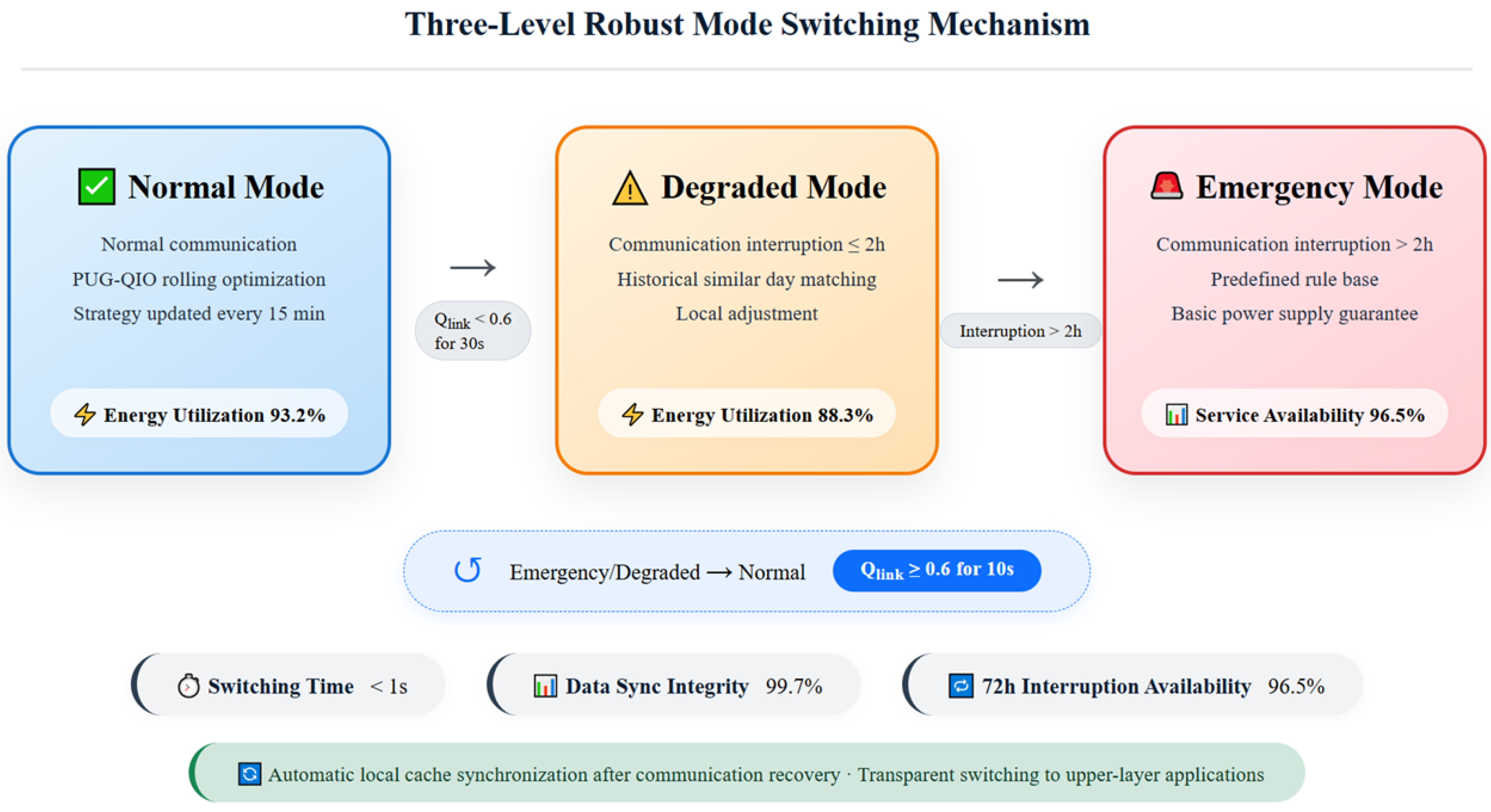
Given weak communication environments, a three-level robust mode-switching mechanism was designed, as illustrated in Figure 7, ensuring basic scheduling capability during communication interruptions.

Normal mode: Communication is normal. Edge nodes receive cloud electricity price signals and weather forecasts. The scheduling algorithm, driven by the latest forecast results, performs rolling optimization every 15 min using the PUG-QIO algorithm, achieving an energy utilization rate of 93.2%.

Degraded mode: Used for communication interruptions lasting ≤2 h. A scenario matching strategy is employed: current moment load and PV output data are compared with historical same-period data; the historical date with highest similarity is selected as a benchmark, and the scheduling scheme is locally adjusted according to current SOC state. Similarity is defined as

$$Sim=\exp \left(-{\displaystyle \frac{\parallel {\mathbf{X}}_{\mathrm{current}}-{\mathbf{X}}_{\mathrm{historical}}{\parallel }^2}{{\sigma }^2}}\right)$$

(16)

where ${\mathbf{X}}_{\mathrm{current}}$ is the characteristic vector of current time, including time (0–23), day type (1–7), past 1 h average load, current irradiance, etc.; ${\mathbf{X}}_{\mathrm{historical}}$ is the characteristic vector of historical date; $\parallel {\mathbf{X}}_{\mathrm{current}}-{\mathbf{X}}_{\mathrm{historical}}{\parallel }^2$ is squared Euclidean distance; and $\sigma =0.5$ is bandwidth parameter controlling similarity decay rate. The exponential function ensures closer distances yield similarities approaching 1, while farther distances yield similarities approaching 0.

The matching process proceeds as follows: From the local history database, retrieve dates with matching season (spring/summer/autumn/winter) and day type (weekday/weekend). Calculate similarity between each historical date and current time. Select the three dates with the highest similarity, take the mean of their scheduling schemes as the benchmark, and adjust the benchmark scheme according to actual SOC (e.g., reduce discharge for low SOC).

Emergency mode: Used for communication interruptions >2 h. Enable preset rule base, executing fixed strategies based on current SOC and time slot type. Example rules:

(1)

If $SOC<0.3$ and PV output $>50$ kW, charge energy storage first, charging power $=min$ (50 kW, PV output).

(2)

If $SOC<0.3$ and PV output $\le 50$ kW, start diesel generator at minimum power (30 kW) to power load and charge energy storage simultaneously.

(3)

If $SOC>0.8$ and load $>100$ kW, priority energy storage discharge, discharge power $=min$ (100 kW, load demand).

(4)

If $SOC>0.8$ and load $\le 100$ kW, energy storage discharge meets load, surplus electricity sold to grid.

(5)

If $0.3\le SOC\le 0.8$ and PV output $>$ load, PV powers load, surplus charges energy storage.

(6)

If $0.3\le SOC\le 0.8$ and PV output $\le$ load, PV + energy storage joint power supply, insufficient portion supplemented by diesel generator.

Rules execute in priority order; subsequent rules are skipped when conditions are met.

Mode-switching triggers: Mode switching is triggered by link quality $Q_{\mathrm{link}}\in \left[\mathrm{0,1}\right]$ (definition see Section 4.2.2). When $Q_{\mathrm{link}}<0.6$ persists for more than 30 s, the system automatically switches mode: normal mode switches to degraded mode (first trigger), and degraded mode upgrades to emergency mode after 2 h. Switching time $<1$ s, transparent to upper layers. After communication restoration, when $Q_{\mathrm{link}}\ge 0.6$ persists for more than 10 s, automatic switch back to normal mode occurs and local cache is synchronized.

The three-level seamless mode-switching mechanism ensures the system maintains the following properties in weak communication environments: 96.5% service availability within 72 h communication interruption, 88.3% energy utilization rate in degraded mode, 0.8 s mode-switching time, and 99.7% data synchronization completeness rate.

4.5. Lightweight Deployment Design

For Raspberry Pi 4B edge node resource constraints, this paper employs the Temporal Sensitivity-Aware Differentiated Pruning (TSADP) strategy to reduce model parameter count from 12.5 M to 4.6 M (63% compression ratio) while maintaining prediction accuracy, supplemented by knowledge distillation to further mitigate accuracy loss. The final deployment model contains 1.2 M parameters, a memory footprint < 500 MB, and single inference time 31 ms.

4.5.1. Temporal Sensitivity-Aware Differentiated Pruning (TSADP)

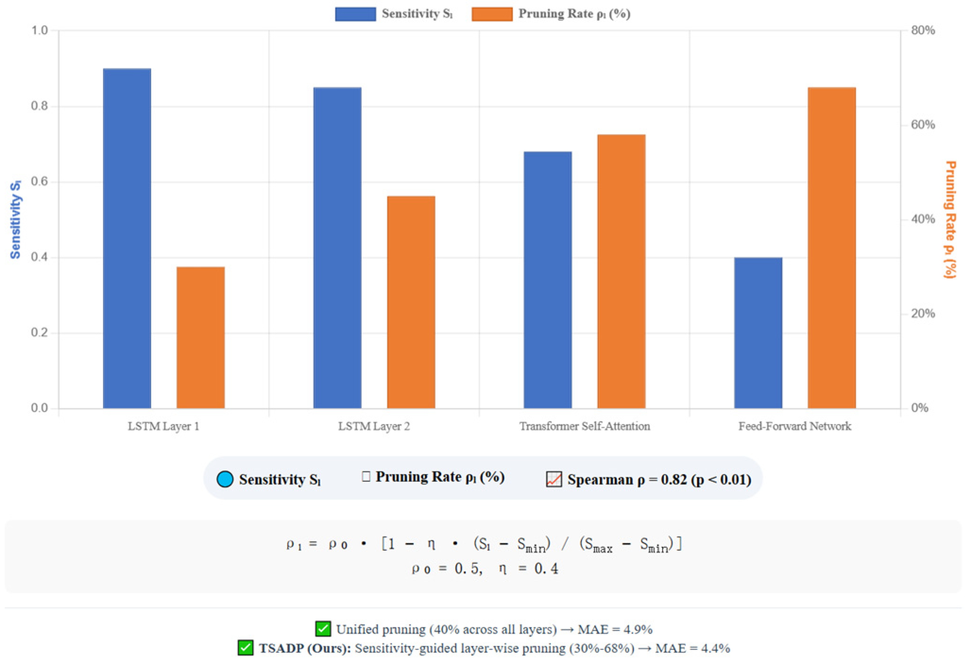
Standard channel pruning for convolutional layers or fully-connected layers using global unified pruning thresholds performs well on image classification tasks, but exhibits structural deficiencies when directly applied to time-series forecasting models: LSTM and Transformer contributions differ significantly across layers for time-series modeling. Shallow feature extraction layers primarily capture local temporal fluctuations; excessive pruning leads to loss of such awareness. Deep aggregation layers, if excessively pruned, struggle to capture global dependencies such as daily cycles. Therefore, this paper proposes the Temporal Sensitivity-Aware Differentiated Pruning (TSADP) strategy, which quantifies each layer’s output impact on prediction loss to achieve “conservative pruning in sensitive layers and aggressive pruning in non-sensitive layers”, as illustrated in Figure 8.

(1)

Temporal Sensitivity Definition

For the trained model, feature perturbation sensitivity is calculated layer by layer on the validation set:

$$S_l={\mathbb{E}}_{{\mathcal{D}}_{\mathrm{val}}}\left[{\parallel {\displaystyle \frac{\partial \mathcal{L}}{\partial {\mathbf{h}}_l}}\parallel }_2\right]$$

(17)

where $\partial {\mathbf{h}}_l$ is layer $l$ output feature; $\partial \mathcal{L}$ is prediction loss; and ${\mathbb{E}}_{{\mathcal{D}}_{\mathrm{val}}}$ represents expectation over the entire validation set. The physical meaning of sensitivity $S_l$ is the degree of impact on final prediction loss when a small perturbation occurs in this layer’s output. Higher sensitivity indicates more important layers where more channels should be reserved.

Does gradient sensitivity represent “temporal sensitivity”? Gradient-based sensitivity has been widely used to measure channel importance in image tasks. However, in time-series prediction, gradient information primarily reflects local loss function change rates on outputs, and may not fully capture layers crucial for maintaining global structure (periodicity, trend) of time series. For example, some layers may not have large gradients to loss function, but their output features carry critical periodic information in the time dimension. Removing these layers leads to prediction curve distortion. To verify positive correlation between gradient sensitivity and temporal importance, a small-scale experiment was conducted on the validation set: for each layer, gradient sensitivity was calculated separately, then all channels of the layer were individually zeroed (simulating complete removal), and mean absolute error increment on validation set (denoted $∆{MAE}_l$) was measured. Results show the Spearman rank correlation coefficient between $S_l$ and $∆{MAE}_l$ is 0.82 (p < 0.01), confirming gradient-based layer sensitivity effectively reflects importance in time-series forecasting tasks. Therefore, using $S_l$ as pruning basis is reasonable and effective.

(2)

Differentiated Pruning Rate

An adaptive pruning rate is set for each layer based on sensitivity:

$${\rho }_l={\rho }_0\left(1-\eta \cdot {\displaystyle \frac{S_l-S_{\mathrm{m}\mathrm{i}\mathrm{n}}}{S_{\mathrm{m}\mathrm{a}\mathrm{x}}-S_{\mathrm{m}\mathrm{i}\mathrm{n}}}}\right)$$

(18)

where ${\rho }_0=0.5$ is the base pruning rate; $\eta =0.4$ is the adjustment coefficient; and $S_{\mathrm{m}\mathrm{i}\mathrm{n}}$, $S_{\mathrm{m}\mathrm{a}\mathrm{x}}$ are minimum and maximum sensitivity values across layers. When $S_{\mathrm{m}\mathrm{a}\mathrm{x}}=S_{\mathrm{m}\mathrm{i}\mathrm{n}}$, ${\displaystyle \frac{S_l-S_{\mathrm{m}\mathrm{i}\mathrm{n}}}{S_{\mathrm{m}\mathrm{a}\mathrm{x}}-S_{\mathrm{m}\mathrm{i}\mathrm{n}}}}=0$ is defined. This design ensures highest-sensitivity layers have lowest pruning rates (~30%), lowest-sensitivity layers have highest pruning rates (~70%), implementing a differentiated strategy.

(3)

Pruning Execution with Fine-Tuning

Pruning execution process: First, evaluate channel importance. For convolutional layers, use BN layer scaling factor $\gamma$ as the channel importance score. $\gamma$ values approaching 0 indicate channel output is suppressed, with lower importance. For fully-connected layers, use L2 norm of weight matrix $W$ as importance score; larger norms indicate greater channel impact on subsequent layers. For each layer, sort channels by importance score from high to low, keep top $1-{\rho }_l$ percentage channels, generating 0–1 mask matrix. Pruning removes weights and biases where mask is 0. Final step updates network structure, with next layer input dimensions adjusted accordingly.

After pruning completion, fine-tuning training is performed to recover accuracy loss from pruning. In the fine-tuning stage, a regularization term is introduced to constrain pruning rate:

$${\mathcal{L}}_{\mathrm{finetune}}={\mathcal{L}}_{\mathrm{original}}+\beta \sum _l{\rho }_l|{\mathit{W}}_l{|}_2$$

(19)

where ${\mathcal{L}}_{\mathrm{original}}$ is the original loss function (mean squared error); $\beta ={10}^{-5}$ is the regularization coefficient; ${\rho }_l$ is pruning rate for layer $l$; and $|{\mathbf{W}}_l{|}_2$ is L2 norm of layer $l$ weights.

Fine-tuning employs Adam optimizer, learning rate ${10}^{-4}$, 20 training epochs, with early stopping based on validation set loss not decreasing for 3 epochs.

4.5.2. Knowledge Distillation and Model Compression

Knowledge distillation is introduced on top of pruning. After pruning (4.6M parameters), the model serves as teacher network to train a more compact student network, further compressing model scale.

Student network structure:

A three-layer stacked LSTM is used, with 64 hidden layer dimensions, 8 input dimensions, and 24 output dimensions (prediction for next 24 h). Specific structure:

(1)

LSTM Layer 1: Input 8 dimensions, hidden layer 64 dimensions, return sequences

(2)

LSTM Layer 2: Input 64 dimensions, hidden layer 64 dimensions, return sequences

(3)

LSTM Layer 3: Input 64 dimensions, hidden layer 64 dimensions, return last moment output

(4)

Fully-connected layer: 64 → 24 dimensions

Student network parameter count is approximately 1.2 M, 26% of teacher network (4.6 M).

Distillation loss function:

The distillation loss function contains hard label loss and soft label loss:

$${\mathcal{L}}_{\mathrm{distill}}=\alpha {\mathcal{L}}_{\mathrm{hard}}\left(y,{\widehat{y}}_s\right)+\left(1-\alpha \right){\mathcal{L}}_{\mathrm{soft}}\left({\widehat{y}}_t,{\widehat{y}}_s\right)$$

(20)

where $y$ is true value (hard label); ${\widehat{y}}_s$ is student network prediction; ${\widehat{y}}_t$ is teacher network prediction (soft label); ${\mathcal{L}}_{\mathrm{hard}}$ is mean squared error (MSE); and ${\mathcal{L}}_{\mathrm{soft}}$ uses KL divergence to measure output distribution differences.

Soft label generation:

Teacher network generates soft labels under temperature parameter $T=3$:

$$q_i={\displaystyle \frac{\exp \left(z_i/T\right)}{{\sum }_j\exp \left(z_j/T\right)}}$$

(21)

where $z_i$ is teacher network output. Temperature parameter $T>1$ makes probability distribution smoother, retaining similarity information between categories.

KL divergence calculation:

$${\mathcal{L}}_{\mathrm{soft}}=T^2\sum _i{p}_i^t\log {\displaystyle \frac{p_i^t}{p_i^s}}$$

(22)

where $p_i^t$ is teacher network soft label probability; $p_i^s$ is student network soft label probability. Multiplication by $T^2$ scale preserves gradient magnitude.

Balance coefficient:

$\alpha =0.3$ was determined by grid search over $[0.1,0.9]$ with step 0.1, selecting minimum validation set MAE. $\alpha =0.3$ means 30% of loss function comes from hard labels (true values), 70% from soft labels (teacher network output).

Training configuration:

(1)

Optimizer: Adam

(2)

Learning rate: ${10}^{-3}$

(3)

Batch size: 32

(4)

Training epochs: 50

(5)

Early stopping: validation set loss not decreasing for 5 epochs

(6)

Hardware: NVIDIA RTX 3090, training time approximately 1 h

4.5.3. Edge Deployment Scheme

After two-stage compression through pruning and distillation, the final distilled student network serves as the deployment model. Model metrics are shown in

Table 4. Comparison of performance metrics before and after model lightweighting.

Indicators	Original Model	After Pruning	Pruning + Distillation (Final Deployment)
Parameter count	12.5 M	4.6 M	1.2 M
Compression ratio	—	63%	90%
Inference time (Raspberry Pi 4B)	85 ms	52 ms	31 ms
Memory footprint	820 MB	430 MB	458 MB
Load forecasting MAE	4.2%	4.4%	4.5%
PV forecasting MAE	4.8%	5.0%	5.1%

.

The final deployment model parameter count is 9.6% of the original model, with inference speed improved by 63% (85 ms → 31 ms), memory footprint <500 MB, satisfying Raspberry Pi 4B deployment requirements. Accuracy loss is only 0.3 percentage points (4.2% → 4.5%), remaining within the design target (≤4.5%).

Deployment architecture:

Model is deployed on Raspberry Pi 4B in TensorFlow Lite format, loaded through C++ API:

(1)

Model conversion: Python 3.9.7-trained Keras model → TensorFlow Lite Converter → .tflite file

(2)

Quantization: Dynamic range quantization (weights from float32 to float16) further reduces model size

(3)

Deployment: C++ program loads .tflite model, performs inference using TensorFlow Lite C++ API

(4)

Input/output: Input is $864\times 8$ float array; output is 24-dimension float array

Runtime monitoring:

Real-time monitoring of inference time and memory usage during system operation:

(1)

Normal state: inference time < 50 ms, memory footprint < 500 MB

(2)

Alert state: inference time > 80 ms or memory usage > 600 MB for 1 min, triggering alarm

(3)

Emergency state: inference time > 120 ms or memory footprint > 800 MB, automatically switch to standby ARIMA prediction model (lightweight, no neural network)

Standby model:

ARIMA (2, 1, 2) model serves as emergency backup:

(1)

Parameter count: <10 KB

(2)

Inference time: <5 ms

(3)

Memory footprint: <10 MB

(4)

Prediction MAE: ~7.5% (lower precision, but ensures basic functionality)

Startup guardian:

(1)

System boot script managed by systemd, set to auto-start on boot

(2)

When process exits abnormally, automatic restart with up to 3 retry attempts

(3)

Key logs recorded in local files to facilitate troubleshooting

5. System Implementation and Experiments

5.1. Development Environment and Tools

The system development and experimental environment spans three tiers: model training, edge deployment, and back-end services.

Model training: Server configuration: Intel Xeon Gold 5218 processor (manufactured by Intel Corporation, Santa Clara, CA, USA) (16 cores, 32 threads), 128 GB memory, NVIDIA RTX 3090 GPU (24 GB memory), Ubuntu 20.04 LTS operating system. Deep learning frameworks: TensorFlow 2.10 and PyTorch 1.12.

Edge deployment: Raspberry Pi 4B, ARM Cortex-A72 quad-core processor (manufactured by ARM Ltd., Cambridge, UK) (1.5 GHz), 4 GB LPDDR4 memory, 64 GB microSD card storage, Raspberry Pi OS (64-bit) operating system. Edge-side algorithms deployed via TensorFlow Lite 2.10.

Back-end services: Tencent Cloud lightweight application server, 2 cores, 4 GB memory, 80 GB SSD, CentOS 7.9 operating system. Service-side framework: Spring Boot 2.7, databases: MySQL 8.0 and Redis 6.2.

5.2. Core Module Implementation

Data acquisition module: Implemented in Python. Modbus RTU devices use pySerial library polling; CAN bus devices are parsed through python-can; the LoRa module receives weather station data in gateway mode. All raw data, after timestamp alignment, is written to a local SQLite database.

Prediction module: The AGDN network was prototyped in PyTorch. Training employed the Adam optimizer with learning rate 1 × 10⁻³, batch size 32, and early stopping patience of 5 epochs. Lightweight implementation proceeded in two steps: first, channel pruning in TensorFlow with model reconstruction, exporting a SavedModel after pruning; then, knowledge distillation to train the student network; finally, conversion to TensorFlow Lite format.

Scheduling module: The quantum-inspired optimization algorithm was implemented in Python, with a population size of 50 and maximum 200 iterations. The fitness function called the DEAP library’s constraint processing module; parallel computing used a multiprocessing Pool divided into five sub-populations for evaluation. The robust mode-switching mechanism was implemented as an independent thread, detecting the communication state every second.

System integration: Each module runs as a separate process on the Raspberry Pi 4B; inter-process communication uses shared memory combined with ZeroMQ. Systemd manages system startup scripts, configured for auto-start and auto-recovery.

5.3. Experimental Dataset and Evaluation Metrics

Experimental data originate from actual operation records of a rural revitalization demonstration area microgrid between January 2022 and June 2023. The microgrid comprises a 300 kWp photovoltaic array, a 200 kW/400 kWh lithium iron phosphate energy storage system, a 150 kW diesel generator, and mixed loads. Data are stored in CSV format, spanning 18 months, resampled to 5 min intervals, totaling approximately 180,000 time-series records. Each record contains 38 fields; core fields include three-phase active power, photovoltaic array DC power, energy storage SOC, and energy storage charge/discharge power.

The dataset is divided chronologically:

(1)

Training set: January–December 2022 (70%)

(2)

Validation set: January–March 2023 (15%)

(3)

Test set: April–June 2023 (15%)

The forecasting horizon is 24 h with a 5 min sampling interval, resulting in 288 time points. No aggregation or resampling was applied to the raw data.

Evaluation Metrics

Forecasting accuracy is evaluated using the following:

(1)

$\mathrm{MAE}={\displaystyle \frac{1}{n}}{\sum }_{i=1}^n\mid y_i-{\widehat{y}}_i\mid$

(2)

$\mathrm{MAPE}={\displaystyle \frac{100\%}{n}}{\sum }_{i=1}^n\mid {\displaystyle \frac{y_i-{\widehat{y}}_i}{y_i}}\mid$

(3)

$\mathrm{RMSE}=\sqrt{{\displaystyle \frac{1}{n}}{\sum }_{i=1}^n(y_i-{\widehat{y}}_i{)}^2}$

(4)

$\mathrm{nRMSE}={\displaystyle \frac{\mathrm{RMSE}}{y_{\max }-y_{\min }}}\times 100\%$

Scheduling performance is evaluated using:

(1)

Energy utilization rate: ${\eta }_{\mathrm{util}}={\displaystyle \frac{{\sum }_{t=1}^T\mathrm{m}\mathrm{i}\mathrm{n}(P_t^{\mathrm{load}},P_t^{\mathrm{PV}}+P_t^{\mathrm{ESS},\mathrm{dis}})}{{\sum }_{t=1}^T{P}_t^{\mathrm{PV}}}}\times 100\%$

(2)

Comprehensive cost: $C_{\mathrm{total}}={\sum }_{t=1}^T\left(c_{\mathrm{dg}}{P}_t^{\mathrm{dg}}\Delta t+c_{\mathrm{buy}}{P}_t^{\mathrm{buy}}\Delta t-c_{\mathrm{sell}}{P}_t^{\mathrm{sell}}\Delta t\right)$

Lightweighting effectiveness is measured by parameter count, inference time (ms), and memory footprint (MB). Real-time response is measured by end-to-end delay (seconds).

5.4. Experimental Results and Analysis

5.4.1. Forecasting Performance Comparison

AGDN was compared on the test set against single LSTM, single Transformer, a TCN–Transformer fusion model, and two advanced lightweight time-series forecasting models: SCINet and DLinear. All models used identical training and validation sets, with an input window of 72 h and output forecasting for the next 24 h. To ensure fairness, SCINet and DLinear followed their original papers’ recommended configurations, with parameter counts adjusted to a similar order of magnitude as AGDN (approximately 1–2 M).

As shown in

Table 5. Comparison of forecasting performance across different models.

	Load MAPE (%)	Load RMSE (%)	PV MAE (%)	PV RMSE (%)	Params (M)	Inference Time (ms)
LSTM	5.2 ± 0.3	6.8 ± 0.4	6.1 ± 0.4	7.5 ± 0.5	0.8	42
Transformer	4.8 ± 0.2	6.3 ± 0.3	5.7 ± 0.3	7.1 ± 0.4	4.2	68
TCN-Transformer	4.5 ± 0.2	5.9 ± 0.3	5.3 ± 0.3	6.8 ± 0.4	3.5	56
SCINet	4.6 ± 0.2	6.0 ± 0.3	5.4 ± 0.3	6.9 ± 0.4	1.8	35
DLinear	4.9 ± 0.3	6.4 ± 0.4	5.8 ± 0.4	7.3 ± 0.5	0.5	12
AGDN (scalar weighting)	4.4 ± 0.2	5.7 ± 0.3	5.1 ± 0.3	6.5 ± 0.4	2.1	48
AGDN (gated fusion)	4.2 ± 0.2	5.3 ± 0.3	4.8 ± 0.3	6.1 ± 0.4	2.2	49

Note: The parameter counts reported for AGDN (2.2M) refer to the compressed deployment model after pruning and distillation (see Section 4.5). The original unpruned AGDN model contains 12.5M parameters.

, AGDN achieves a load forecasting MAE of 4.2%, representing the following:

(1)

18.7% reduction compared to LSTM (5.2%);

(2)

12.3% reduction compared to Transformer (4.8%);

(3)

6.7% reduction compared to TCN–Transformer (4.5%).

Compared with advanced lightweight models, AGDN accuracy exceeds SCINet (4.2% vs. 4.6%) and DLinear (4.2% vs. 4.9%), with a parameter count (2.2 M) comparable to SCINet (1.8 M) and slightly higher than DLinear (0.5 M). Inference time for AGDN is 49 ms, slightly higher than SCINet (35 ms), but remains well within the system’s real-time requirement (end-to-end delay ≤ 10 s), while offering a significant prediction accuracy advantage (0.4 percentage point lower load MAE). This demonstrates AGDN’s comprehensive advantages in the accuracy–efficiency trade-off.

Figure 9 illustrates load forecasting results for a typical week (15–21 May 2023). In the scenario of a transient load drop caused by sudden rainfall on 17 May, LSTM response lags by approximately 2 h; Transformer captures the abrupt change but exhibits large fluctuations; AGDN achieves smoother tracking of the abrupt change while maintaining overall trend fitting accuracy.

Ablation Study: To verify the effectiveness of the gated fusion mechanism, three fusion methods were designed for comparison:

(1)

Scalar weighting: $\widehat{\mathrm{y}}=\mathsf{\alpha }\cdot \mathrm{LSTM}\left(\mathrm{X}\right)+\left(1-\mathsf{\alpha }\right)\cdot \mathrm{Transformer}\left(\mathrm{X}\right)$, with $\mathsf{\alpha }=0.6$ determined by grid search.

(2)

Concatenation + fully-connected: LSTM and Transformer outputs are concatenated and passed through a two-layer fully-connected network for nonlinear fusion.

(3)

Gated fusion (this paper): Dynamic weighted fusion at the feature-dimension level.

Table 6. Ablation study: Comparison of different fusion approaches.

Fusion Approach	Load MAE (%)	PV MAE (%)	Parameter Increment (K)
Scalar weighting	4.4	5.1	0
Concatenation + FC	4.3	5.0	28.4
Gated fusion	4.2	4.8	32.9

shows that gated fusion outperforms simple scalar weighting (0.2 percentage point lower load MAE) and concatenation + fully-connected nonlinear fusion (0.1 percentage point lower load MAE). This demonstrates that dynamic feature-dimension-level weight allocation enables finer integration of both branches’ advantages. In terms of parameter increment, gated fusion adds only 32.9K parameters (9.6% of total), comparable to concatenation + fully-connected, but with more significant performance improvement.

5.4.2. Scheduling Effectiveness Analysis

Three scheduling policies were compared:

(1)

Baseline strategy: No forecasting, fixed rules;

(2)

Standard quantum-inspired algorithm: Fixed rotation angle;

(3)

PUG-QIO (this paper): Adaptive rotation angle guided by prediction uncertainty.

All policies used identical prediction inputs for scheduling simulation.

Table 7. Comparison of scheduling policy effectiveness.

Strategy	Energy Utilization (%)	Fuel Cost (Yuan/Day)	Purchase Cost (Yuan/Day)	Sales Revenue (Yuan/Day)	Comprehensive Cost (Yuan/Day)	Solution Time (s)
Baseline	81.7 ± 2.1	1260 ± 85	320 ± 42	45 ± 12	1535	0.02 (rule lookup)
Standard Quantum	89.5 ± 1.8	1020 ± 62	210 ± 28	68 ± 15	1162	5.8 ± 0.6
PUG-QIO	93.2 ± 1.5	918 ± 48	150 ± 21	82 ± 18	986	5.3 ± 0.5

Note: Comprehensive cost = Fuel cost + Purchase cost − Sales revenue.

shows that PUG-QIO achieves an energy utilization rate of 93.2%—11.5 percentage points higher than the baseline strategy and 3.7 percentage points higher than the standard quantum-inspired algorithm. Average daily fuel cost is 918 yuan, 27.3% lower than the baseline and 10.2% lower than the standard algorithm. In terms of solution time, PUG-QIO averages 5.3 s, slightly faster than the standard algorithm (5.8 s) due to adaptive rotation angle accelerating convergence. Both algorithms meet the system’s 10 s response time limit, while the baseline strategy, though faster, exhibits the worst effectiveness.

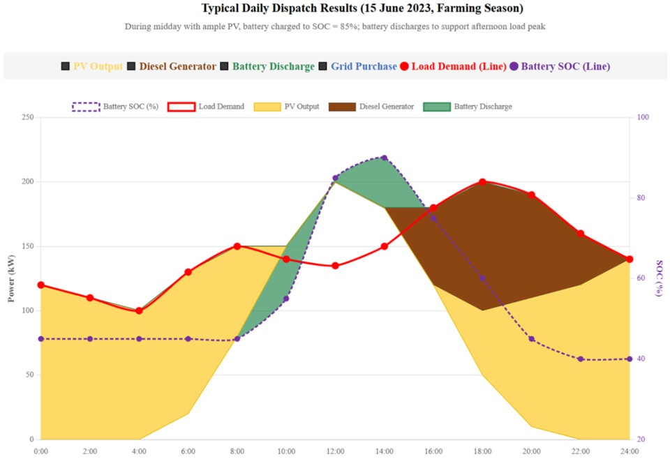
Figure 10 illustrates scheduling results for a typical day (15 June 2023, busy farming season). At noon when PV output is abundant, the baseline strategy’s delayed energy storage charging leads to partial curtailment. Although the standard quantum-inspired strategy charges in advance, its fixed rotation angle causes slow discharge response when the afternoon load spikes. PUG-QIO dynamically adjusts its search strategy according to the prediction confidence interval, charging the energy storage to SOC = 0.85 before the noon PV peak and providing timely discharge support when the afternoon load rises. The daily curtailment rate is only 3.2%, 4.6 percentage points lower than the standard algorithm.

Monte Carlo Robustness Verification: To systematically evaluate PUG-QIO’s robustness against prediction uncertainties, Monte Carlo simulation experiments were designed. On the basis of the original test set predictions, Gaussian noise with different intensities was superimposed to simulate varying degrees of prediction error. Noise intensity was controlled by the Signal-to-Noise Ratio (SNR):

(1)

Low noise: SNR = 20 dB;

(2)

Medium noise: SNR = 15 dB;

(3)

High noise: SNR = 10 dB.

For each noise level, 100 sets of perturbed prediction sequences were independently generated. Scheduling schemes were generated by both the standard quantum-inspired algorithm and PUG-QIO, and the average comprehensive cost and constraint violation rate were measured.

Table 8. Monte Carlo robustness verification results.

Noise Level	SNR	Standard Quantum (Yuan/Day)	PUG-QIO (Yuan/Day)	Cost Reduction	Constraint Violation (PUG-QIO)
Low	20 dB	1195 ± 42	1012 ± 35	15.3%	0%
Medium	15 dB	1287 ± 68	1065 ± 52	17.2%	0.3%
High	10 dB	1452 ± 112	1183 ± 86	18.5%	1.2%

shows that costs for both algorithms increase with noise, but PUG-QIO increases more slowly. Stronger noise yields greater cost reductions for PUG-QIO relative to the standard algorithm (15.3% → 17.2% → 18.5%). The 18.5% cost reduction under high noise fully verifies the core value of the adaptive rotation angle mechanism in handling prediction uncertainty—when prediction confidence is low, the algorithm automatically expands the search range, avoiding local optima caused by unreliable predictions. PUG-QIO’s constraint violation rate is only 1.2% under high noise, much lower than the standard algorithm’s 4.8%, indicating that PUG-QIO has better fault tolerance to prediction errors.

5.4.3. Lightweighting Effectiveness Validation

The following strategies were compared:

(1)

Unified pruning: Fixed threshold $\mathsf{\tau }=0.5$;

(2)

TSADP (this paper): Differentiated pruning based on temporal sensitivity;

(3)

Separate knowledge distillation;

(4)

Separate weight quantization (INT8);

(5)

TSADP + distillation (this paper): Hybrid strategy.

Final deployment models for all schemes must meet Raspberry Pi 4B operational requirements.

Analysis of

Table 9. Comparison of lightweighting strategy effectiveness.

	Params (M)	Compression (%)	Inference (ms)	Memory (MB)	Load MAE (%)	PV MAE (%)
Original model	12.5	—	85	820	4.2 ± 0.2	4.8 ± 0.2
$\mathrm{Unified} \mathrm{pruning} (\mathsf{\tau }=0.5$)	4.6	63%	51	430	4.9 ± 0.3	5.6 ± 0.3
TSADP (this paper)	4.6	63%	52	430	4.4 ± 0.2	5.0 ± 0.2
Separate knowledge distillation	1.2	90%	32	460	4.7 ± 0.2	5.4 ± 0.2
Separate weight quantization (INT8) *	3.1	75%	28	310	4.5 ± 0.2	5.2 ± 0.2
TSADP + distillation (this paper)	1.2	90%	31	458	4.5 ± 0.2	5.1 ± 0.2

* Note: INT8 quantization reduces model storage size from approximately 50 MB to 12.5 MB (a 75% reduction) while keeping the parameter count unchanged (12.5M). The inference speed improves due to reduced memory bandwidth requirements and hardware acceleration support.

:

(1)

Unified pruning increases MAE to 4.9% at 63% compression (0.7 percentage point loss), while TSADP loses only 0.2 percentage points at the same compression ratio (4.2% → 4.4%). The 0.5 percentage point MAE difference fully proves TSADP’s core idea: identifying important layers through temporal sensitivity analysis and implementing differentiated pruning can effectively protect layers critical to temporal modeling (LSTM layers, self-attention layers) and avoid loss of critical temporal information.

(2)

Knowledge distillation alone compresses the model to 1.2 M, but MAE rises to 4.7%, slightly higher than TSADP + distillation (4.5%), indicating that pruning before distillation can mitigate accuracy loss.

(3)

Weight quantization alone (INT8) achieves the fastest inference speed (28 ms) and lowest memory footprint (310 MB), but requires dedicated hardware acceleration, with MAE 4.5% similar to TSADP + distillation.

(4)

The TSADP + distillation hybrid strategy achieves 90% compression, MAE of only 4.5% (meeting the design target of ≤4.5%), inference speed of 31 ms, and memory footprint of 458 MB—the best comprehensive effect.

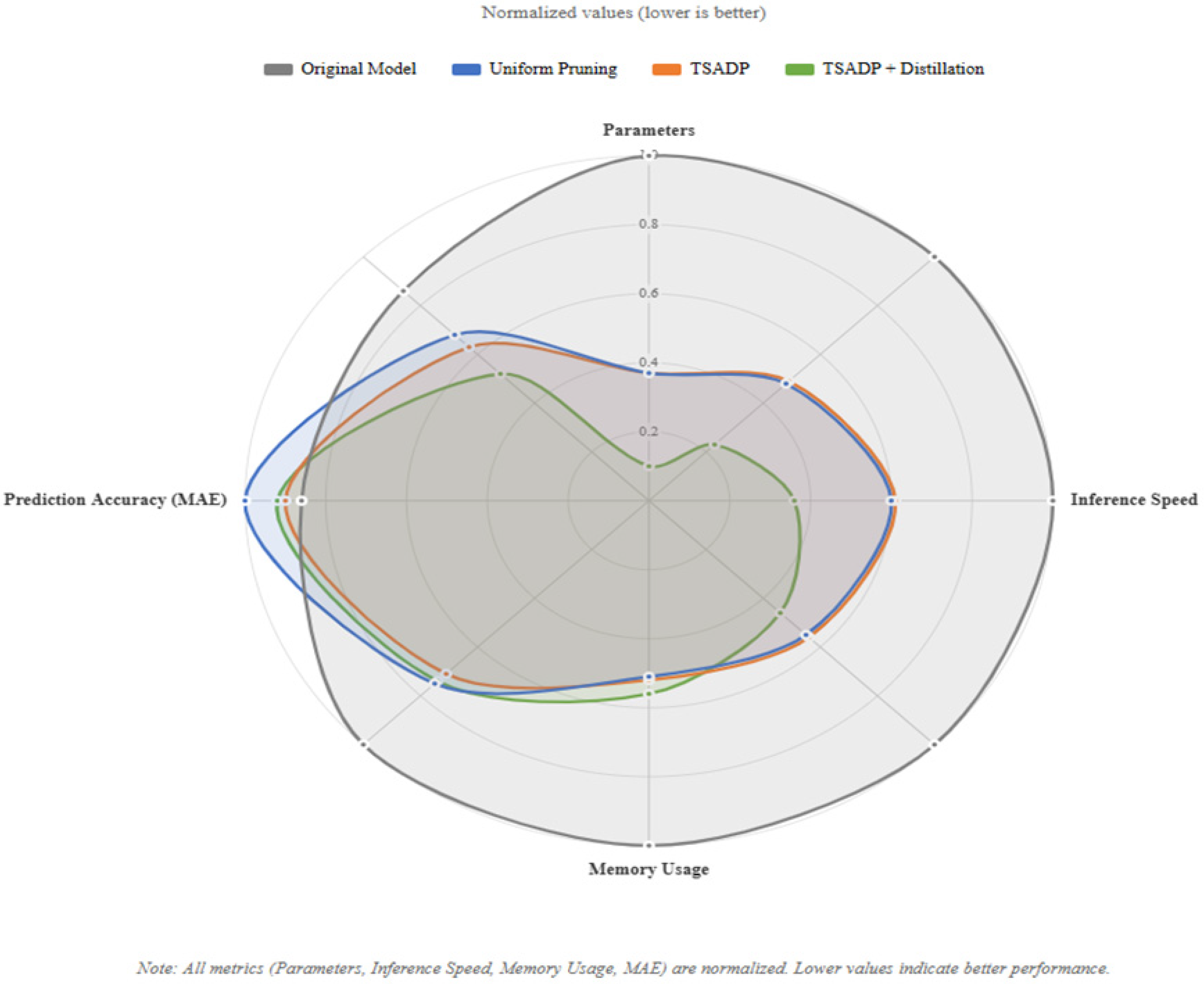
Figure 11 shows the actual pruning rate distribution across layers:

(1)

LSTM layers: Average pruning rate 52%.

(2)

Transformer self-attention layers: Average pruning rate 45%.

(3)

Feedforward network layers: Average pruning rate 68%.

This distribution verifies the differences in layer importance for temporal modeling.

5.4.4. Comprehensive System Performance Evaluation

The system was integrated and deployed at the pilot village microgrid site, with actual operation testing conducted for 30 consecutive days (1–30 July 2023), as shown in Figure 12.

Real-time response: End-to-end delay was continuously recorded for 100 complete scheduling cycles:

(1)

Average: 8.7 s

(2)

P95 delay: 9.8 s

(3)

Maximum delay: 11.2 s

Time breakdown by link:

(1)

Data acquisition and preprocessing: 3.2 s

(2)

Prediction inference: 0.8 s

(3)

Scheduling optimization: 4.1 s

(4)

Instruction issuance and execution: 0.6 s

Weak communication robustness: The 4G module was artificially disconnected for 8 h to simulate communication interruption.

(1)

30 s after interruption: System automatically switched to degraded mode, generating scheduling schemes based on historical similar-day matching.

(2)

After 2 h: System switched to emergency mode, enabling rule-based operation.

(3)

During interruption: Energy utilization rate was 88.3% (4.9 percentage points lower than normal mode), with no system shutdown or equipment misoperation.

(4)

After communication restoration: Local cache data synchronized automatically with 99.7% integrity rate.

Economic calculation basis: Electricity cost savings of 2180 yuan are based on comparison with the manual experience scheduling mode during the same period last year (July 2022).

(1)

July 2022 (before deployment): Diesel consumption ≈ 1362 L; electricity purchase cost ≈ 12,000 yuan.

(2)

July 2023 (system trial): Diesel consumption ≈ 982 L (reduction of 380 L); electricity purchased 1.8 MWh; electricity sales revenue 2460 yuan.

(3)

Diesel price: 8.2 yuan/L (local purchase price).

(4)

Diesel cost savings: 380 L × 8.2 yuan/L ≈ 3116 yuan.

(5)

Net electricity cost savings: After subtracting the net increase in electricity sales revenue (2460 yuan—previous year’s revenue), the net savings are approximately 2180 yuan.

Based on this calculation, the system investment cost is expected to be recovered in 2.3 years, providing a clear decision-making basis for engineering deployment.

Stability: During 30 days of continuous operation:

(1)

Software exceptions: 3 recorded (all repaired)

(2)

Hardware exceptions: 0 recorded

(3)

Mean time between failures: Approximately 240 h

(4)

WARNING-level alarms: 42 recorded, mainly from communication transients (31 times) and sensor data anomalies (11 times)

The system recovered automatically according to the design strategy in all cases, comprehensively demonstrating system reliability in actual rural environments.

6. Conclusions and Future Work

6.1. Research Summary

This paper has addressed the triple constraints of weak communication, low computing power, and strong fluctuations in rural microgrids by designing and implementing an energy management system with forecasting–scheduling co-optimization and edge deployability. The main contributions are summarized as follows:

(1)

Adaptive Gated Dual-stream Network (AGDN): A gated fusion mechanism has been proposed to dynamically balance the contributions of LSTM and Transformer at the feature-dimension level. The load forecasting Mean Absolute Percentage Error (MAPE) reaches 4.2%, representing an 18.7% reduction compared to standalone LSTM.

(2)

Prediction Uncertainty-Guided Quantum-Inspired Optimization (PUG-QIO): An algorithm that maps prediction confidence intervals to quantum rotation angles has been designed to enable adaptive search. The energy utilization rate reaches 93.2%, and the average daily fuel cost of the diesel generator is reduced by 27.3%.

(3)

Temporal Sensitivity-Aware Differentiated Pruning (TSADP): A pruning strategy that maintains forecasting accuracy at a 63% parameter compression ratio has been developed. Combined with knowledge distillation, the final deployment model is compressed to 1.2M parameters (9.6% of the original model), achieving a 63% improvement in inference speed and a memory footprint below 500 MB.

(4)

Field Validation: The system was tested in a real rural microgrid for 30 consecutive days. The end-to-end response delay remained below 10 s. Even under weak communication conditions, the energy utilization rate reached 88.3%, with cumulative electricity cost savings of 2180 yuan—verifying the effectiveness and reliability of the proposed scheme.

6.2. Main Contributions

(1)

Forecasting Level: AGDN achieves fine-grained adaptive fusion of LSTM and Transformer through a gated mechanism, enabling single models to capture multi-scale fluctuation features.

(2)

Scheduling Level: PUG-QIO embeds prediction uncertainty into quantum search, realizing closed-loop co-optimization and increasing energy utilization by 5.7 percentage points under high uncertainty.

(3)

Deployment Level: TSADP introduces temporal sensitivity-guided differentiated pruning, enabling edge deployment of high-precision models on resource-constrained devices.

6.3. Limitations and Future Work

Despite these promising results, this study has several limitations:

(1)

Data Limitations: Multi-source information such as Numerical Weather Prediction (NWP), dynamic electricity pricing, and agricultural activity schedules have not been fully integrated into the forecasting framework. As noted by the reviewer, incorporating these data sources could further enhance forecasting accuracy and robustness. This limitation will be addressed in our future work on multi-source data fusion (Future Work direction 1).

(2)

Algorithmic Limitations: The interpretability of the gating vectors in AGDN requires further analysis. Additionally, the historical similar-day matching algorithm does not adequately account for load profile morphological characteristics.

(3)

Engineering Limitations: The system has not yet been tested under extreme environmental conditions (e.g., severe weather, prolonged communication outages), and the risk of single-point failures has not been fully addressed.

(4)

System Integration Limitations: Adjustable resources (e.g., flexible loads, electric vehicles) are not yet connected, and the potential for multi-microgrid collaboration remains unexplored.

Future Work

Future research will focus on the following three directions:

(1)

Multi-source data fusion: We plan to incorporate Numerical Weather Prediction (NWP), dynamic electricity pricing, and agricultural machinery scheduling into a multi-source fusion framework. Meteorological fluctuations, price peaks, and farming activities will be encoded as auxiliary features and concatenated with original time-series data, enabling the model to anticipate weather evolution and agricultural impacts on load patterns.

(2)

Cross-regional generalization via transfer learning: Transfer learning will encode geographical location, climate zone, and PV resource level as prior knowledge through regional embeddings, allowing the model to dynamically adjust prediction bias according to regional characteristics—enabling rapid adaptation to new areas with minimal fine-tuning samples.

(3)

Federated learning for multi-microgrid collaboration: A federated learning framework will be constructed where each edge node trains locally and uploads only encrypted model parameters to the cloud, eliminating privacy risks. After cloud aggregation, a global prediction model is distributed, enabling coordinated energy storage sharing among multiple microgrids and improving regional renewable energy accommodation.

References

1. Shahzad, S.; Abbasi, M.A.; Ali, H.; Iqbal, M.; Munir, R.; Kilic, H. Possibilities, Challenges, and Future Opportunities of Microgrids: A Review. Sustainability 2023, 15, 6366. [Google Scholar] [CrossRef]
2. Liu, X.; Zhao, T.; Deng, H.; Wang, P.; Liu, J.; Blaabjerg, F. Microgrid Energy Management with Energy Storage Systems: A Review. IEEE Trans. Power Syst. 2025, 40, 1234–1250. [Google Scholar] [CrossRef]
3. Li, J.H. Discussion on the Application and Development of Microgrids in Modern Rural Power Grids. China Electr. Power Enterp. Manag. 2024, 40, 66–68. (In Chinese) [Google Scholar]
4. Qiao, Q. Microgrids Burst with Great Energy. China Electr. Power Enterp. Manag. 2024, 6, 24–26. (In Chinese) [Google Scholar]
5. Habbak, H.; Mahmoud, M.; Metwally, K.; Fouda, M.M.; Ibrahem, M.I. Load Forecasting Techniques and Their Applications in Smart Grids. Energies 2023, 16, 1480. [Google Scholar] [CrossRef]
6. Abumohsen, M.; Owda, A.Y.; Owda, M. Electrical Load Forecasting Using LSTM, GRU, and RNN Algorithms. Energies 2023, 16, 2283. [Google Scholar] [CrossRef]
7. Zhang, W.; Cheng, M.; Xiang, Q.; Li, Q. Enhancing Short-Term Load Forecasting Through K-Shape Clustering and Deep Learning Integration. IEEE Access 2025, 13, 30123–30138. [Google Scholar] [CrossRef]
8. Akhtar, S.; Shahzad, S.; Zaheer, A.; Ullah, H.S.; Kilic, H.; Gono, R.; Jasinski, M.; Leonowicz, Z. Short-Term Load Forecasting Models: A Review of Challenges, Progress, and the Road Ahead. Energies 2023, 16, 4060. [Google Scholar] [CrossRef]
9. Abdelghany, M.B.; Al-Durra, A.; Gao, F. A Coordinated Optimal Operation of a Grid-Connected Wind-Solar Microgrid Incorporating Hybrid Energy Storage Management Systems. IEEE Trans. Sustain. Energy 2024, 15, 39–51. [Google Scholar] [CrossRef]
10. Rangarajan, S.S.; Raman, R.; Singh, A.; Shiva, C.K.; Kumar, R.; Sadhu, P.K.; Collins, E.R.; Senju, T. DC Microgrids: A Propitious Smart Grid Paradigm for Smart Cities. Smart Cities 2023, 6, 1690–1718. [Google Scholar] [CrossRef]
11. Du, M.Z.; Wu, J.L.; Sun, H.Y.; Gao, L.L. Research on Construction and Application of Rural Smart Energy Systems Based on DC Microgrids in the Context of China’s Dual Carbon Goals. J. Shenyang Inst. Eng. (Nat. Sci. Ed.) 2025, 21, 1–8. (In Chinese) [Google Scholar]
12. Chen, J.; Wang, S.S.; Ying, D.X.; Fan, X.C.; Shi, R.J.; Zhu, R.W.; Li, J. Electricity Empowers Smart Agriculture and Helps Rural Revitalization: A Case Study of Grapes in Turpan, Xinjiang. Appl. Energy Technol. 2022, 6, 1–4. (In Chinese) [Google Scholar]
13. Jing, X.W.; Fu, Y. Tongzhou: Microgrid System Empowers Beautiful Countryside. China Electr. Power Enterp. Manag. 2024, 6, 27–29. (In Chinese) [Google Scholar]
14. Che, Y.Y.; Liu, L.T.; Fang, B.M.; Fan, R.M.; Zhao, X. Coordinated Optimal Operation Strategy of Wind-Solar Microgrid Hybrid Energy Storage System Based on Model Predictive Control. Hydropower Energy Sci. 2025, 11, 172–178. (In Chinese) [Google Scholar]
15. Yan, Y.H. Discussion and Research on Serving “Village Revitalization” Grid-Connected Optical Storage Microgrid Technology. Ningxia Electr. Power 2021, 5, 38–40. (In Chinese) [Google Scholar]
16. Eyimaya, S.E.; Altin, N.; Nasiri, A. Optimization of Photovoltaic and Battery Storage Sizing in a DC Microgrid Using LSTM Networks Based on Load Forecasting. Energies 2025, 18, 3676. [Google Scholar] [CrossRef]
17. Dewangan, F.; Abdelaziz, A.Y.; Biswal, M. Load Forecasting Models in Smart Grid Using Smart Meter Information: A Review. Energies 2023, 16, 1404. [Google Scholar] [CrossRef]
18. Chen, Y.; Wan, K.; Zhao, J.; Yu, M. Accurate Consensus-Based Distributed Secondary Control with Tolerance of Communication Delays for DC Microgrids. Int. J. Electr. Power Energy Syst. 2024, 155, 109636. [Google Scholar] [CrossRef]
19. Tomás-Martín, A.; Kazemtabrizi, B.; García-Cerrada, A.; Sigrist, L.; Bueno, E.J. Decentralised Consensus-Based Hierarchical Control of a Hybrid AC-DC Microgrid Robust to Communication Delays. Int. J. Electr. Power Energy Syst. 2026, 175, 111645. [Google Scholar] [CrossRef]
20. He, P.; Zhu, Y.; Tao, Y.; Liu, X.; Shao, J. Frequency Control Strategy of Microgrid Distributed Virtual Synchronous Generator Based on Asynchronous Event Triggered Communication Protocol. Int. J. Electr. Power Energy Syst. 2025, 168, 110666. [Google Scholar] [CrossRef]
21. Fu, D.; Miao, G.X.; Wang, X.; Yuan, L.; Sun, H.R.; Chen, Y.W.; Li, Z.X.; Wang, X.H. Robust Optimal Scheduling Strategy for Agricultural Microgrid Containing Small Pumped Storage Plant. Hydropower Energy Sci. 2025; in press. (In Chinese)
22. Lei, J.; Liu, Z. Nested Bi-level Scheduling Strategy for Energy Storage Systems in Hybrid Microgrid Considering Uncertainties of Battery Dynamic Performances. Int. J. Electr. Power Energy Syst. 2025, 166, 110575. [Google Scholar] [CrossRef]
Figure 1. The triple constraints of rural microgrids and their coupling effects on EMS.
Energies 19 01910 g001
Figure 2. Development context of temporal forecasting technologies [9,10,11,12,13,14,15].
Energies 19 01910 g002
Figure 3. Classification of optimization scheduling methods [1,2,4,6,7,8].
Energies 19 01910 g003
Figure 4. Overall system architecture.
Energies 19 01910 g004
Figure 5. Structure of Adaptive Gated Dual-stream Network (AGDN).
Energies 19 01910 g005
Figure 6. Schematic diagram of the gated fusion mechanism.
Energies 19 01910 g006
Figure 7. Diagram of three-stage robust mode-switching mechanism.
Energies 19 01910 g007
Figure 8. Diagram of Temporal Sensitivity-Aware Differentiated Pruning (TSADP) strategy.
Energies 19 01910 g008
Figure 9. Comparison of typical weekly load forecasting performance.
Energies 19 01910 g009
Figure 10. Stacked area chart of typical daily scheduling results (drawn by the authors based on experimental data).
Energies 19 01910 g010
Figure 11. Radar chart comparing lightweighting strategy effectiveness.
Energies 19 01910 g011
Figure 12. Bar chart of 30-day economic comparison during trial operation.
Energies 19 01910 g012