The Physical Cost of a Complete Substitution of Fossil Fuels

Abstract

Proposals for the complete substitution of fossil fuels have become central to energy policy debates. However, historical data show that global primary energy consumption has grown approximately linearly since the 1950s, with changes in the energy mix occurring mainly through diversification rather than absolute substitution. This work examines the physical and operational constraints of complete substitution proposals by grounding the analysis in the observed evolution of global energy use and in a dynamical framework of system adequacy and stability. A normalized model balancing firm capacity, intermittency, and corrective power was developed and applied to four 20-year scenarios: (A) constant demand with diversification, (B) continued linear demand growth, (C1) fossil-fuel phase-out at constant demand, and (C2) phase-out with continued growth. The results show that gradual diversification remains within operationally ordered regimes, whereas rapid phase-out trajectories approach or cross stability boundaries associated with supply–demand bifurcations. Quantitative estimates indicate that full substitution over two decades requires cumulative additional energy investments on the order of ${10}^6$ TWh, corresponding to total system costs of US$50–100 trillion under conservative assumptions. These costs arise from the cumulative energetic and entropic burdens of maintaining operational order in increasingly complex and intermittent systems. Our analysis indicates that rapid fossil-fuel substitution over short time horizons is constrained not only by technology or finance but also by cumulative energy investment, entropy production, and erosion of operational stability margins.

1. Introduction

The large-scale organization of modern societies rests on the continuous availability of dense, reliable, and controllable energy flows. Over the past century, fossil fuels—particularly oil—have played a central role in providing not only energy but also the material, logistical, and temporal stability required to sustain complex industrial systems. In recent years, the rapid expansion of alternative energy sources has often been discussed in terms of substitution or phase-out narratives. Recent proposals advocating for the complete substitution of fossil fuels have become central to contemporary energy debates [1].

However, empirical evidence shows that new energy sources have historically been added to the global energy system rather than replacing existing ones [2]. From a physical perspective, energy systems are therefore better understood as evolving structures of increasing diversity and complexity, in which different carriers perform distinct functional roles. This raises a fundamental question that remains insufficiently addressed: what are the energetic, entropic, and dynamical costs associated with expanding and diversifying the energy supply while preserving system-level operational order and stability?

Despite the breadth of energy policy proposals, the dominant framing remains primarily emissions- and policy-centric. Less frequently addressed are the physical constraints that arise even under an idealized, carbon-free substitution, as any useful energy ultimately degrades into heat, which generates entropy; therefore, enforcing operational order—firmness, reliability, and predictability—over an energy system dominated by intermittency requires additional layers of storage, redundancy, control, and transmission, with each of these introducing irreversible losses.

Furthermore, from a physical standpoint, large-scale energy transformations are constrained by irreversibility and entropy production, which are concepts long established in thermodynamics and economic theory [3,4]. In this regard, classical results in complexity and control theory show that increasing system size and structural complexity tend to reduce global stability margins, even in the presence of enhanced local control [5,6,7,8,9].

In other words, those proposals do not necessarily eliminate dissipation; instead, they might redistribute it and, in some configurations, may amplify the total entropy production as a direct consequence of maintaining operational order. In fact, previous studies examined the adequacy, firm capacity, and storage requirements in systems with high shares of variable generation [10,11,12,13,14,15,16,17,18,19], but a physically grounded analysis of cumulative energy and entropic costs associated with rapid full substitution remains limited.

This study contributes a complementary perspective: we analyzed the physical cost of complete fossil-fuel substitution scenarios, emphasizing (i) the irreducible thermodynamic minimum associated with final energy use, (ii) the additional entropy production required to enforce operational order in intermittent-dominated networks, and (iii) a supply–demand bifurcation that separates an operational ordered regime (achieved at higher dissipative cost) from an unstable regime characterized by persistent deficits and cascading failures. The goal is not to dispute mitigation objectives, but to clarify that any proposal to abolish fossil fuels must confront fundamental thermodynamic and dynamical limits, in addition to policy, finance, and technology issues.

In this work, the terms alternative energies and other energies are used to denote all primary energy sources that are not fossil-based. This definition intentionally differs from the narrower concept of renewable energy, as it includes non-fossil but non-renewable sources such as nuclear power or traditional biomass. The distinction is essential for the present analysis, which focuses on the physical and operational consequences of replacing fossil fuels, independent of the renewability classification of the substitute sources.

Moreover, we restrict the analysis to a 20-year horizon, as this timeframe corresponds to the 2050 benchmarks, which are commonly adopted in energy policy and transition scenarios. Therefore, this yields a direct comparison between physical constraints and prevailing policy expectations.

A large body of research has examined pathways for deep decarbonization of the global energy system using detailed techno-economic models, including integrated assessment models (IAMs), capacity expansion models, and power system optimization frameworks. These approaches explicitly represent technological portfolios, regional heterogeneity, infrastructure deployment, and policy constraints to explore possible decarbonization trajectories [20,21,22].

Numerous studies have used these models to investigate highly renewable or fully decarbonized energy systems [23,24]. While these models provide valuable insights into technological deployment pathways and economic trade-offs, they typically operate at high levels of structural and parametric complexity. The objective of the present work is complementary. Rather than reproducing the full technological and regional structure of the global energy system, this study developed a reduced physical framework aimed at identifying fundamental energetic and dynamical constraints associated with large-scale substitution processes.

By combining historical energy consumption trends; thermodynamic considerations; and a simplified adequacy model that captures the balance between firm capacity, intermittency, and corrective mechanisms, the analysis focuses on the cumulative energetic effort required to maintain operational order in increasingly complex energy systems. In this sense, the proposed framework should be interpreted not as a substitute for detailed techno-economic modeling but as a complementary perspective highlighting system-level physical constraints that may remain less visible in highly detailed scenario models.

2. Historical Growth of Global Energy Consumption

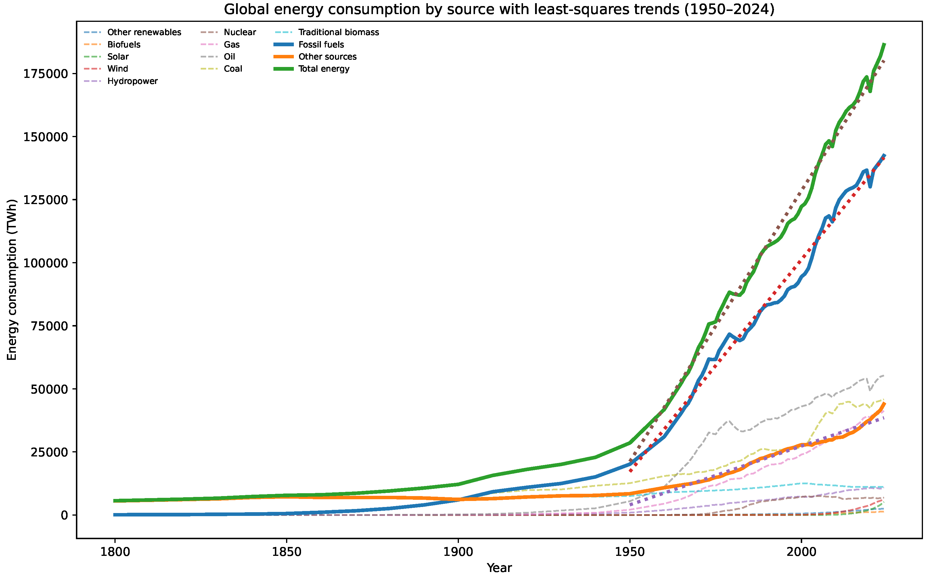
Any discussion of a complete substitution of fossil fuels must be grounded in the empirical evolution of global energy consumption. Figure 1 summarizes the long-term trajectory of total primary energy use, together with the contributions from fossil fuels and other sources, over the past six decades. The figure is based on consolidated data from harmonized series made available by Our World in Data series [2].

Two robust features emerge from the data shown in Figure 1. First, global energy consumption has grown in a remarkably steady and almost monotonic manner since the 1950s. Despite oil shocks, economic crises, geopolitical disruptions, and successive waves of technological change, total primary energy use exhibits a persistent upward trend. This growth closely tracks population increase, industrialization, electrification, and rising per-capita energy demand. The long-term regularity of the curve suggests that global energy consumption is driven primarily by structural socio-economic factors, rather than by short-term fluctuations in energy prices or by the availability of specific fuels.

Second, the expansion of non-fossil energy sources has not resulted in an absolute decline in fossil fuel use. Instead, alternative sources have grown largely in parallel with fossil fuels, contributing to the increase in total energy supply rather than displacing existing consumption. Indeed, fossil fuel consumption has continued to rise in absolute terms, even during periods of rapid deployment of renewable sources and other low-carbon technologies [2].

Accordingly, the total global primary energy consumption is approximately $186\times {10}^3$ TWh per year. Fossil fuels account for roughly $142\times {10}^3$ TWh per year, or about 76% of the global total, while all other sources combined contribute approximately $44\times {10}^3$ TWh per year. These values highlight a central empirical fact: alternative energy sources have not yet achieved the large-scale substitution of fossil fuels but have primarily served to satisfy incremental demand growth in a process recently named energy addition [1].

Figure 1 provides a compact empirical synthesis of the recent evolution of the global energy system, which is central to the argument developed in this work. Over the last six decades, the data reveal that non-fossil sources have grown steadily, but largely as an additive contribution to total supply, without inducing an absolute decline in fossil ones.

Moreover, the least-squares trends highlighted for fossil sources, other sources, and total energy exhibit an almost linear growth regime from 1950 onward. This near-linearity indicates that despite successive waves of public policies, market interventions, and technological deployment aimed at reshaping the energy mix, their net effect on aggregate consumption trajectories has remained limited. At the system level, fossil and non-fossil sources have continued to scale in parallel, while the total energy demand follows a structurally robust growth path. This empirical regularity underscores that the core challenge is not merely compositional change, but the physical expansion of the energy system itself caused by the high demand of the emerging technological society.

The near-linear growth of total energy consumption observed over the last 70 years further implies that substitution is unlikely to occur against a background of stable or declining demand. Instead, it must contend with a continuously expanding and highly demanding global energy system. Consequently, the central challenge is not whether alternative sources can grow rapidly in relative terms, but whether they can grow fast enough in absolute terms to replace the existing fossil baseline while simultaneously accommodating additional demand.

This empirical backdrop motivates the analysis developed in the following sections. Anchoring the discussion in long-run consumption data clarifies that the problem of complete fossil-fuel substitution scenarios is fundamentally quantitative and physical. It is against this historical trajectory—characterized by persistent growth and the absence of absolute substitution—that the thermodynamic, entropic, and dynamical limits explored in this work must be assessed. This persistent growth trajectory sets a lower bound on the thermodynamic and entropic costs that any large-scale energy reconfiguration must confront.

3. Operational Order Enforcement and Additional Entropy Production

The analytical framework adopted in this work intentionally relies on a reduced representation of the global energy system. The objective is not to reproduce the full technological, geographical, and economic complexity of modern energy infrastructures, which is typically addressed through large-scale techno-economic optimization models. Instead, the model captures a limited set of system-level variables governing operational adequacy in energy networks: firm dispatchable capacity, statistical variability of intermittent generation, and corrective mechanisms required to maintain the supply–demand balance.

Reduced models of this type are widely used in the analysis of complex physical systems to identify stability conditions and scaling relationships that may be obscured in highly detailed simulations. Within this perspective, the probabilistic adequacy condition derived in this section should be interpreted as a minimal representation of the reliability constraints that any energy system must satisfy. The purpose of this abstraction is therefore analytical rather than predictive: it enables the identification of general physical relationships between intermittency, corrective effort, entropy production, and cumulative energy investment, independent of the specific technological configuration of future energy systems.

For an amount of energy Q degraded at an effective temperature T, the minimum entropy generated is [3,4,25]

$$\Delta S_{min}={\displaystyle \frac{Q}{T}}.$$

(1)

This expression represents a strict lower bound imposed by the Second Law of Thermodynamics that is independent of the mode of energy production. Therefore, a substitution of fossil fuels that preserves the total energy consumption cannot reduce this baseline entropy production.

In fact, for present-day global energy use, this thermodynamic floor corresponds to entropy production in the order of ${10}^{18} \mathrm{J} {\mathrm{K}}^{-1}$ per year. Any realistic discussion of energy substitution must hence distinguish between unavoidable entropy associated with final energy use and additional entropy generated by system organization.

It is important to emphasize that intermittent energy sources require mechanisms to ensure temporal matching between supply and demand. These mechanisms include energy storage, redundancy of capacity, real-time control, forecasting, and grid reinforcement. Each introduces irreversible processes.

In this framework, the total internal entropy production rate of the system, i.e., $S_i^{\mathrm{tot}}$, can be decomposed as [4]

$${\dot{S}}_i^{\mathrm{tot}}={\dot{S}}_i^{\mathrm{gen}}+{\dot{S}}_i^{\mathrm{grid}}+{\dot{S}}_i^{\mathrm{stor}}+{\dot{S}}_i^{\mathrm{ctrl}},$$

(2)

where the terms on the right side of the equation represent the entropy production associated with energy conversion ($S_i^{\mathrm{gen}}$), transmission losses ($S_i^{\mathrm{grid}}$), storage cycles ($S_i^{\mathrm{stor}}$), and control or information processing ($S_i^{\mathrm{ctrl}}$).

Additionally, for storage, which is central to intermittency management, entropy production is approximately [14,16]

$${\dot{S}}_i^{\mathrm{stor}}\approx {\displaystyle \frac{(1-{\eta }_{\mathrm{rt}}) P_{\mathrm{cyc}}}{T}},$$

(3)

where ${\eta }_{\mathrm{rt}}$ is the round-trip efficiency and $P_{\mathrm{cyc}}$ is the mean power processed by storage. Increasing the reliability requires increasing $P_{\mathrm{cyc}}$, thereby increasing the entropy production.

Supply–Demand Bifurcation and Stability Boundary

Consider a system supplying an instantaneous demand $D\left(t\right)$, which was previously met by fossil fuels. After substitution, the supply $Su\left(t\right)$ can be written as

$$Su\left(t\right)=F+I\left(t\right)+B\left(t\right),$$

(4)

where F denotes the firm dispatchable capacity, $I\left(t\right)$ denotes the aggregated intermittent generation, and $B\left(t\right)$ denotes the net storage output. Thus, the instantaneous deficit $\Delta \left(t\right)$ is given by [10,11]

$$\Delta \left(t\right)=D\left(t\right)-Su\left(t\right).$$

(5)

Moreover, the operational order can be defined probabilistically as [10,11]

$$Pr[\Delta (t)>0]\le \epsilon ,$$

(6)

with $\epsilon$ being a tolerated risk level.

The stored energy $E\left(t\right)$ evolves according to [15,16]

$${\displaystyle \frac{dE\left(t\right)}{dt}}={\eta }_c{P}_c\left(t\right)-{\displaystyle \frac{1}{{\eta }_d}}{P}_d\left(t\right)-\lambda E\left(t\right),$$

(7)

where $0\le E\left(t\right)\le E_{max}$; $P_d$ denotes the instantaneous corrective, i.e., dispatchable, power activated to compensate short-term imbalances between the generation and demand; and $P_c$ represents the available corrective capacity or, more specifically, the maximum fast-response power that can be mobilized through storage discharge, reserves, demand response, or emergency dispatch.

On dispatch timescales, intermittent generation may be approximated as [11,13]

$$I\left(t\right)={\mu }_I+{\sigma }_{I}Z,Z\sim \mathcal{N}(0,1),$$

(8)

where $I\left(t\right)$ denotes the aggregated instantaneous output of non-dispatchable generation, ${\mu }_I$ is its mean value, ${\sigma }_I$ is its standard deviation, and Z is a standard normal random variable ($Z\sim \mathcal{N}(0,1)$) representing normalized stochastic fluctuations of intermittent supply. In subsequent expressions, the lowercase symbol z denotes the corresponding deterministic quantile of the same distribution, defined by $Pr(Z\le z)=1-\epsilon$, and represents the safety factor associated with the target reliability level.

Thus, the reliability condition becomes [10,12,13]

$$F+{\mu }_I+P_{d,max}\ge \overline{D}+z_{1-\epsilon } {\sigma }_I,$$

(9)

where F denotes the installed firm (dispatchable) generation capacity, $P_{d,max}$ is the maximum available fast-response corrective power, ${\sigma }_I$ represents the effective standard deviation of non-dispatchable generation, $\epsilon$ is the tolerated probability of supply–demand imbalance, and $z_{1-\epsilon }$ is the corresponding quantile of the standard normal distribution defining the required reliability margin.

For substitution scenarios in which ${\mu }_I\approx \overline{D}$, this equation reduces to

$$F+P_{d,max}\ge z_{1-\epsilon } {\sigma }_I.$$

(10)

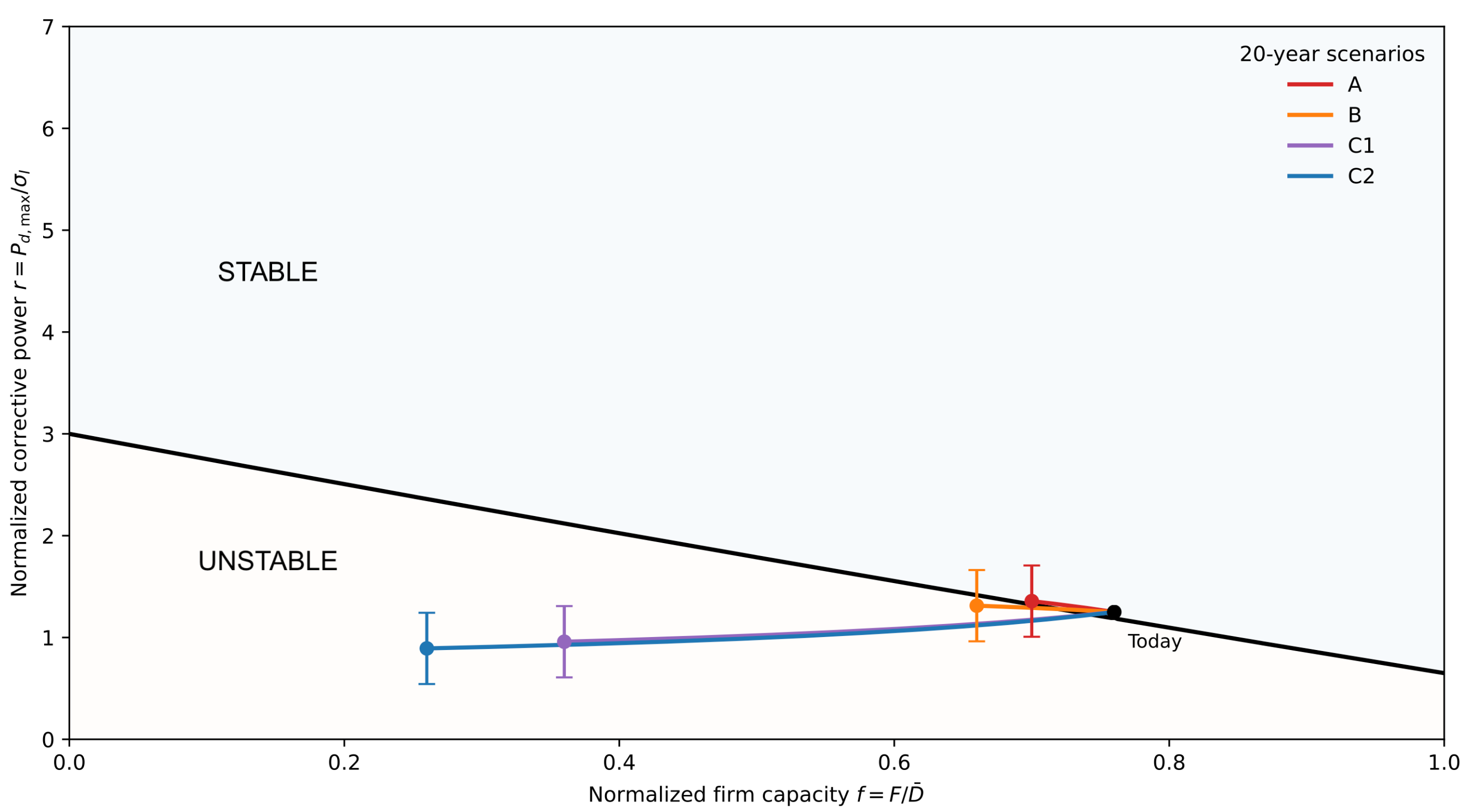
Here, equality defines a critical boundary separating two regimes. Above it, deficits are rare and the system operates in an operational ordered regime. Below it, deficits become frequent and systemic. This transition constitutes a supply–demand bifurcation governed not by linear instability but by storage power saturation and stored energy exhaustion. Figure 2 shows the phase diagram of operational stability.

Equations (9) and (10) define a necessary condition for operational adequacy in terms of the balance between the firm capacity F, corrective power $P_{d,max}$, and statistical variability ${\sigma }_I$ of non-dispatchable generation. This inequality naturally defines a boundary in the reduced phase space spanned by the normalized variables $f=F/\overline{D}$ and $r=P_{d,max}/{\sigma }_I$. Rather than introducing additional assumptions, this representation provides a compact geometrical interpretation of the reliability condition already derived above, highlighting how reductions in firm capacity must be compensated for by increasing corrective power to preserve operational order.

Moreover, it is important to emphasize that, on the one hand, reducing firm capacity requires large increases in storage and control, thereby increasing entropy production, while on the other hand, maintaining operational order requires continuous forecasting, dispatch, and decision-making. Each logically irreversible operation dissipates a minimum energy given by the Landauer bound [26],

$$E_{min}=k_{B}Tln2.$$

(11)

Although real systems operate far above this limit, it establishes a fundamental constraint, i.e., perfect substitution without dissipation is physically impossible.

4. Entropic Effects over a 20-Year Horizon

In this section, our analysis is grounded in the historical trends shown in Figure 1, which reveal a quasi-linear increase in global primary energy consumption since the mid-twentieth century. Based on these data, we consider three physically well-defined scenarios. Scenario A assumes constant total energy demand over the analysis horizon, isolating the cost of system reconfiguration without expansion; Scenario B follows a continuation of the historical least-squares trend, in which the total energy demand grows linearly while combining diversification with system expansion; and Scenario C represents a qualitatively distinct case in which the fossil fuel energy supply is reduced to zero over the same horizon and fully replaced by non-fossil sources, thereby removing a major source of firm capacity and introducing additional dynamical constraints not present in Scenarios A and B.

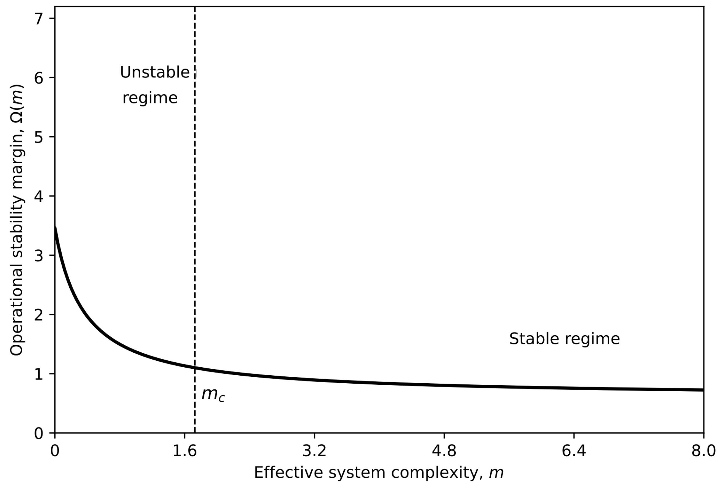
For the sake of clarity, we analyze the scenarios that can be interpreted as distinct trajectories in the phase space shown in Figure 2, which summarizes the physical stability structure of the energy system in terms of the firm capacity, intermittency, storage, and control, while Figure 3 provides a complementary and more abstract representation of the dynamical transition between ordered and unstable regimes. In this sense, the scenarios analyzed henceforth can be interpreted as explicit time-dependent trajectories constrained by the stability structure derived in Section 3 and summarized geometrically in Figure 2 and Figure 3.

It is important to emphasize that while the phase-space representation of Figure 2 captures the operational balance between firmness, intermittency, and corrective effort, it does not explicitly address the structural origin of the growing control burden under substitution. This structural aspect is clarified by considering the effective complexity of the energy system. As additional new generation technologies, storage layers, control mechanisms, and spatial couplings are introduced to enforce reliability, the system dimensionality increases, reducing its global stability margins. In this regard, Figure 3 provides a complementary representation of this stability–complexity trade-off, grounding the phase-space dynamics of Figure 2 in well-established results from nonlinear systems and control theory.

The probabilistic adequacy condition derived in Section 3 implicitly defines a finite stability margin for the energy system. For given values of the firm capacity, intermittency, and corrective power, there exists a maximum admissible perturbation amplitude in the demand or supply fluctuations that could be absorbed without triggering persistent deficits or cascading failures.

In Figure 3, we denote this maximum admissible perturbation amplitude by $\Omega \left(m\right)$, where m represents the effective structural and dynamical complexity of the system. In this context, $\Omega \left(m\right)$ is a compact representation of the tolerance implied by Equations (9) and (10) after the number of interacting technologies, control layers, storage mechanisms, spatial couplings, and stochastic inputs is taken into account.

To complement the thermodynamic and dynamical analysis developed in the previous section, we now introduce explicit near-term scenarios aimed at quantifying the energetic and entropic costs associated with large-scale energy system reconfiguration over a 20-year horizon. This time window is the usual horizon planned as net zero while remaining anchored in empirically observed growth regimes rather than long-term speculative extrapolations.

4.1. Scenario A: Constant Total Energy Demand

In the first scenario, the total global primary energy consumption is assumed to remain constant over the next 20 years at its present level:

$$E_0\simeq 1.86\times {10}^5 \mathrm{TWh} {\mathrm{yr}}^{-1},$$

(12)

where $E_0$ denotes the annual global final energy consumption.

Under this assumption, the deployment of alternative energy sources does not correspond to net system expansion, but rather to an internal reallocation of supply while preserving total throughput.

Even in this idealized case, enforcing system-level operational order in a diversified energy system entails an intrinsic energetic overhead. Indeed, alternative energy sources generally require additional infrastructure, buffering, control, and redundancy to provide levels of firmness and reliability comparable with those of established firm energy carriers. We therefore introduce a dimensionless overhead parameter $\xi$ to represent this requirement, which corresponds to the additional annual energetic cost associated with order enforcement, as follows:

$$\Delta E_{\mathrm{ord}}=\xi E_0.$$

(13)

Using a conservative estimate of $\xi \simeq 0.10$, this yields

$$\Delta E_{\mathrm{ord}}\simeq 1.86\times {10}^4 \mathrm{TWh} {\mathrm{yr}}^{-1}.$$

(14)

An important parameter in the present analysis is the dimensionless overhead factor $\xi$, which represents the additional energetic effort required to maintain operational order in energy systems with increasing shares of intermittent generation. Physically, this overhead reflects the combined energetic cost associated with the buffering, reserve capacity, storage cycling, transmission expansion, forecasting, and real-time balancing required to maintain supply–demand adequacy.

Empirical studies of high-renewable power systems consistently show that these system-integration mechanisms introduce additional system costs typically ranging between approximately 5% and 20%, depending on the renewable penetration levels and system flexibility [22,23,24,27].

Because these system costs ultimately reflect additional infrastructure deployment, operational reserves, storage operation, and balancing requirements, they imply an associated increase in system-level energetic throughput.

In this context, the baseline value adopted in this study ($\xi \approx 0.10$;

Table 1. Representative estimates of system integration costs associated with high shares of variable renewable energy reported in the literature. These costs include grid expansion, balancing reserves, storage deployment, and operational flexibility mechanisms.

Study	Analyzed System	Additional System Cost
Ueckerdt et al. (2013) [23]	Global modeling	5–15%
Hirth (2013) [24]	European power systems	5–20%
Denholm & Hand (2011) [27]	US power systems	∼10%
IEA World Energy Outlook	Global scenarios	10–20%

) represents a conservative order-of-magnitude estimate located near the lower bound of the range reported in the literature. The analysis therefore primarily focuses on the scaling behavior of cumulative energetic requirements with respect to $\xi$, rather than on a precise numerical prediction.

The associated entropy production rate scales as

$${\dot{S}}_{\mathrm{ord}}\sim {\displaystyle \frac{\Delta E_{\mathrm{ord}}}{T}},$$

(15)

where T denotes an effective system temperature characterizing dissipation. Thus, over a 20-year horizon, the cumulative entropic cost in this scenario will be

$$S_{\mathrm{cum}}^{\left(A\right)}\sim {\displaystyle \frac{20 \Delta E_{\mathrm{ord}}}{T}},$$

(16)

which shows that even in the absence of demand growth, large-scale growth necessarily incurs a finite and irreversible entropic burden arising purely from the maintenance of operational order.

In this scenario, the cumulative entropy production scales proportionally with the additional corrective effort required to accommodate diversification, which remains consistent with the operationally ordered regime defined in Section 3.

4.2. Scenario B: Linear Growth of Total Energy Demand

In the second scenario, we assume that the total energy demand continues to grow linearly, following the historical least-squares trend identified in Figure 1. Over the period 1950–2024, this trend corresponds to an average increase of approximately

$$\alpha \simeq 2.15\times {10}^3 \mathrm{TWh} {\mathrm{yr}}^{-1}.$$

(17)

Over the following 20 years, this implies an additional annual throughput of

$$\Delta E_{\mathrm{growth}}=20 \alpha \simeq 4.3\times {10}^4 \mathrm{TWh} {\mathrm{yr}}^{-1},$$

(18)

with a cumulative added energy flow of approximately

$$E_{\mathrm{cum}}^{\mathrm{growth}}\simeq 4.3\times {10}^5 \mathrm{TWh}.$$

(19)

In this case, the energetic cost of maintaining operational order must be evaluated for an expanding system. The total additional energetic burden associated with order enforcement can be approximated as

$$\Delta E_{\mathrm{tot}}=\xi \left(E_0+\Delta E_{\mathrm{growth}}\right),$$

(20)

This leads to a cumulative entropy production over 20 years of

$$S_{\mathrm{cum}}^{\left(B\right)}\sim {\displaystyle \frac{20 \xi \left(E_0+\Delta E_{\mathrm{growth}}\right)}{T}}.$$

(21)

This expression highlights that the dominant contribution to entropy production arises not from the replacement of one energy carrier by another, but from the physical expansion of the energy system itself. Energy diversification amplifies this effect by increasing the coordination, control, and buffering requirements necessary to preserve operational order across heterogeneous energy sources.

The entropic cost in this case reflects not only diversification overheads but also the sustained expansion of system scale, leading to higher cumulative entropy production while preserving operational adequacy.

4.3. Scenario C: Complete Fossil-Fuel Phase-Out over 20 Years

We now analyze a stringent substitution pathway in which fossil fuel energy consumption declines linearly to zero over a 20-year horizon, while non-fossil (“other”) sources expand to fully replace the fossil contribution. This scenario represents the strongest possible form of large-scale energy substitution and is often implicitly assumed in proposals for complete fossil-fuel elimination [1].

At present, the total global primary energy consumption is given by

$$E_0\simeq 1.86\times {10}^5 \mathrm{TWh} {\mathrm{yr}}^{-1},$$

(22)

of which non-fossil sources account for

$$E_{\mathrm{other},0}\simeq 4.40\times {10}^4 \mathrm{TWh} {\mathrm{yr}}^{-1},$$

(23)

with the remainder supplied by fossil fuels. A complete phase-out therefore requires that non-fossil sources reach the full system demand within two decades. Because the trajectory of total demand is uncertain, we consider two explicit sub-scenarios.

4.3.1. Scenario C1: Constant Total Energy Demand

In the first sub-scenario, we assume that the total annual energy demand will remain constant at its present level:

$$E_{\mathrm{tot}}\left(t\right)=E_0\mathrm{for}0\le t\le 20.$$

(24)

Under this hypothesis, non-fossil sources would increase from $E_{\mathrm{other},0}$ to $E_{\mathrm{other}}\left(20\right)\to E_0$. The required net increase in annual non-fossil output will therefore be

$$\Delta E_{\mathrm{C}1}=E_0-E_{\mathrm{other},0}\simeq 1.42\times {10}^5 \mathrm{TWh} {\mathrm{yr}}^{-1}.$$

(25)

Assuming a linear ramp over 20 years, the implied deployment rate will be

$${\beta }_{\mathrm{C}1}={\displaystyle \frac{\Delta E_{\mathrm{C}1}}{20}}\simeq 7.1\times {10}^3 \mathrm{TWh} {\mathrm{yr}}^{-2}.$$

(26)

Although an explicit entropy balance is not written in this case, the energetic cost of complete substitution implicitly includes a substantially larger entropic burden. The rapid replacement of firm capacity by intermittent sources requires intensified cycling of storage, reserves, and control systems so that entropy production grows superlinearly relative to Scenarios A and B, which is consistent with the stability constraints derived in Section 3.

4.3.2. Scenario C2: Linearly Increasing Total Energy Demand

In the second sub-scenario, the total energy demand continues to grow linearly, which is consistent with the historical least-squares trend identified in Figure 1. We shall adopt a growth rate of

$$\alpha =2147 \mathrm{TWh} {\mathrm{yr}}^{-2},$$

(27)

and thus, the total demand evolves as

$$E_{\mathrm{tot}}\left(t\right)=E_0+\alpha t,\hspace{1em}{E}_{\mathrm{tot}}\left(20\right)=E_0+20\alpha .$$

(28)

After 20 years, this yields

$$E_{\mathrm{tot}}\left(20\right)\simeq 2.29\times {10}^5 \mathrm{TWh} {\mathrm{yr}}^{-1}.$$

(29)

Full substitution then requires non-fossil sources to reach the same level, implying a net increase of

$$\Delta E_{\mathrm{C}2}=\left(E_0+20\alpha \right)-E_{\mathrm{other},0}\simeq 1.85\times {10}^5 \mathrm{TWh} {\mathrm{yr}}^{-1}.$$

(30)

Thus, the corresponding linear deployment rate becomes

$${\beta }_{\mathrm{C}2}={\displaystyle \frac{\Delta E_{\mathrm{C}2}}{20}}\simeq 9.3\times {10}^3 \mathrm{TWh} {\mathrm{yr}}^{-2},$$

(31)

which substantially exceeds both the historical growth of non-fossil sources in Scenarios A and B, as well as the rate required in the constant-demand case.

When fossil-fuel phase-out is combined with continued demand growth, the energetic and entropic burdens become inseparable. The cumulative energy investment quantified above necessarily entails elevated entropy production, reflecting the increased corrective effort required to sustain operational order near or beyond the stability boundary.

Table 2. Summary of the 20-year energy system scenarios analyzed in Section 4. This table compares the demand evolution, substitution dynamics, energetic and entropic implications, and proximity to operational stability boundaries for each scenario.

Scenario	Demand Evolution	Energy Mix Dynamics	Energetic and Entropic Implications	Stability Regime
A	Constant total demand	Gradual diversification; fossil capacity retained	Moderate additional energy investment; entropy production increases proportionally to corrective effort	Operationally ordered; stability margins preserved
B	Linear growth of total demand	Diversification with expanding system scale	Higher cumulative energy investment; entropy production grows with both scale and variability	Ordered but closer to stability boundary
C1	Constant total demand	Complete fossil-fuel phase-out over 20 years	Large cumulative energy investment; strong increase in entropy production due to loss of firm capacity and intensified corrective action	Approaches or crosses stability boundary
C2	Linear demand growth	Fossil-fuel phase-out combined with continued growth	Maximum cumulative energy and entropic burden; superlinear corrective effort required to maintain adequacy	High risk of bifurcation and operational instability

highlights that the critical distinction between the scenarios lies not in the average energy supply, but in the cumulative energetic and entropic effort required to preserve operational order under different substitution pathways.

4.3.3. Order-Enforcement Burden and Stability Considerations

We can see that in both sub-scenarios, the required ramp rates ${\beta }_{\mathrm{C}1}$ and ${\beta }_{\mathrm{C}2}$ exceed the historical expansion rate of non-fossil energy observed over recent decades by an order of magnitude, indicating that this pathway constitutes a regime shift rather than a continuation of past trends.

Moreover, the elimination of fossil fuels removes a major source of firm and dispatchable capacity, directly affecting the adequacy condition derived in Section 3. As the firm capacity F is explicit in Equation (10), its reduction cannot be treated as a marginal perturbation. To preserve operational stability, firm capacity loss must be compensated for by a large escalation in corrective mechanisms, including storage power, storage duration, redundancy, and control effort. This requirement follows directly from the stability condition, which can be expressed as

$$F+P_{d,max}\ge z_{1-\epsilon } {\sigma }_I.$$

(32)

As $F\to 0$, this compensation requirement intensifies, forcing the system toward the instability boundary.

The additional energetic overhead $\Delta E_{\mathrm{ord}}^{\left(C\right)}$ associated with maintaining operational order in this fully substituted architecture can be represented as

$$\Delta E_{\mathrm{ord}}^{\left(C\right)}={\xi }_{\mathrm{sub}} E_{\mathrm{tot}},$$

(33)

where ${\xi }_{\mathrm{sub}}>\xi$ reflects an increase in buffering and coordination demands an intermittency-dominated system. Over a 20-year horizon, the cumulative overhead $Q_{\mathrm{cum}}^{\left(C\right)}$ should therefore satisfy

$$Q_{\mathrm{cum}}^{\left(C\right)}=20 {\xi }_{\mathrm{sub}} {\overline{E}}_{\mathrm{tot}},$$

(34)

with ${\overline{E}}_{\mathrm{tot}}=E_0$ in Scenario C1 and ${\overline{E}}_{\mathrm{tot}}=E_0+10\alpha$ in Scenario C2.

These expressions highlight that a rapid, complete substitution of fossil fuels compounds large-scale energetic deployment with increased entropic cost, accelerating the approach to the system-level point of no return identified in the dynamical analysis.

4.4. Implications for System Stability

The results obtained in Scenarios A, B, and C can be interpreted coherently within the phase-space representation introduced in Figure 2, which provides a compact dynamical summary of the trade-offs between the firm capacity, intermittency, storage power, and control effort required to maintain operational order.

In Scenario A, where the total energy demand is held constant, diversification of supply primarily increases the system heterogeneity without expanding the mean demand. In the language of Figure 2, this corresponds to a gradual displacement within the operationally ordered region, moving the system closer to the bifurcation boundary as the normalized firm capacity f decreases and the compensatory storage and control requirements r increase. Although the system remains stable, this is accomplished at the cost of the elevated dissipation and entropy production associated with order enforcement.

Scenario B introduces a continued linear growth of total energy demand on top of this diversification. In phase-space terms, this combines a reduction in effective firm margin with an outward expansion of the system scale. The corresponding trajectory in Figure 2 approaches the stability boundary more rapidly, as the increase in demand amplifies the corrective power and storage requirements needed to satisfy the reliability condition. This explains why the cumulative entropic cost in Scenario B exceeds that of Scenario A, even for identical values of the overhead parameter $\xi$.

Scenario C represents a qualitatively distinct regime. A progressive removal of fossil fuels while increasing the other sources eliminates a major source of firm and dispatchable capacity, consequently producing an abrupt vertical displacement in the phase diagram. As $f\to 0$, maintaining the operational order requires large increases in storage power, duration, redundancy, and control. In this limit, the system is forced toward the bifurcation boundary identified in Figure 2, beyond which small perturbations in supply or demand lead to frequent deficits and cascading failures. The additional energetic overhead introduced in Scenario C is therefore not merely additive, but reflects the proximity to a dynamical instability.

Taken together, these interpretations clarify that the entropic and energetic costs are not arbitrary modeling artifacts, but direct manifestations of the stability structure of the energy system. The phase diagram highlights that large-scale energy substitution trajectories differ not only in magnitude, but in dynamical character, i.e., Scenarios A and B approach the stability boundary from within the ordered regime, whereas Scenario C systematically erodes the stabilizing mechanisms that define the regime.

The estimates in

Table 3. Energetic and social cost scenarios associated with entropy production over a 20-year horizon. The table reports cumulative energetic overheads that arise from order enforcement in a diversified energy system for different values of the dimensionless overhead parameter $\xi$. The total current global primary energy consumption is taken as $E_0\simeq 1.86\times {10}^5$ TWh yr⁻¹. The cumulative additional energy was computed as $Q_{\mathrm{cum}}=20 \xi E_0$. The monetary costs correspond to a conservative lower-bound estimate assuming an average system cost of USD 50 MWh⁻¹.

$\mathit{\xi }$	${\mathit{Q}}_{\mathbf{cum}}$ (TWh)	Cost (USD Trillion)	Practical Implication
0.05	$1.86\times {10}^5$	9.3	Moderate pressure on tariffs and public investment
0.10	$3.72\times {10}^5$	18.6	System-wide institutional and fiscal stress
0.20	$7.44\times {10}^5$	37.2	Severe regressive impact and energy-access constraints

were calculated by adopting a deliberately conservative but physically grounded approach to estimate order-of-magnitude bounds and their source parameters.

The sensitivity analysis summarized in

Table 4. Sensitivity of cumulative energetic costs to the assumed average system-level cost per unit of energy. Results are shown for a representative overhead parameter $\xi =0.10$ over a 20-year horizon. The cumulative additional energy is $Q_{\mathrm{cum}}=3.72\times {10}^5$ TWh, computed from $Q_{\mathrm{cum}}=20 \xi E_0$ with $E_0\simeq 1.86\times {10}^5$ TWh yr⁻¹.

Cost per MWh (USD)	${\mathit{Q}}_{\mathbf{cum}}$ (TWh)	Total Cost (USD Trillion)
30	$3.72\times {10}^5$	11.2
50	$3.72\times {10}^5$	18.6
100	$3.72\times {10}^5$	37.2

indicates that even under conservative assumptions for the average system-level cost per unit of energy, the resulting cumulative expenditures remain in the multi-trillion-dollar range.

Within this, two parameters dominate the uncertainty of the cumulative cost: the dimensionless overhead factor $\xi$, which captures the energetic burden associated with enforcing operational order, and the average system-level cost per unit of energy. Importantly, the qualitative conclusions of this analysis are robust with respect to reasonable variations in both parameters.

Because the cumulative additional energy scales linearly with $\xi$ as $Q_{\mathrm{cum}}\to 20$, even modest values of the overhead factor lead to substantial energetic requirements over a 20-year horizon. For example, reducing $\xi$ by a factor of two proportionally reduces the cumulative energetic burden, but does not alter its order of magnitude. This linear dependence implies that uncertainty in $\xi$ affects the cost scale, but not the existence of a significant entropic burden associated with large-scale system reconfiguration.

A second source of uncertainty arises from the monetary valuation of the additional energy dissipated in maintaining operational order. To assess the sensitivity of the results to this parameter, Table 4 reports cumulative costs for a representative value $\xi =0.10$ under different assumptions for the average system cost per megawatt-hour. Even under conservative cost estimates, the resulting cumulative expenditures remain in the multi-trillion-dollar range over two decades. Higher cost assumptions, which may be more representative of firm capacity, storage, and reliability services, may further amplify this effect.

Taken together, these considerations indicate that the central result of this work is structurally clear: the energetic and social costs associated with increased entropy production are not an artifact of particular parameter choices, but a direct consequence of enforcing operational order in a growing and increasingly heterogeneous energy system.

5. Discussion

The results presented in this work enable a quantitative assessment of large-scale energy substitution that goes beyond capacity accounting and focuses on physical and operational constraints. By combining historical consumption data, explicit dynamic formulations, and scenario-based projections, the analysis clarifies how energy diversification and fossil-fuel substitution interact with system-level stability, corrective effort, and entropy production.

Figure 1 establishes the empirical starting point: global primary energy consumption has increased quasi-linearly over the last six decades, while changes in the energy mix occurred primarily through diversification rather than net substitution. The trends fitted by mean squared error show that both fossil and non-fossil sources grew in absolute terms since the 1950s, and that the slope of the total curve remained largely insensitive to compositional changes. This observation is critical for the scenario analysis because it implies that substitution policies must operate on top of a large and persistent energy flow, rather than on a shrinking baseline. In practical terms, the historical record supports the interpretation that diversification has been easier to realize than full displacement, which is consistent with the persistent dominance of fossil-derived energy at the global scale.

Section 3 introduced a dynamical framework in which adequacy is governed by the balance between firm capacity, variability of non-dispatchable generation, and corrective power. Figure 3 makes this balance explicit by representing the system state in the phase space, while including a stability boundary derived from standard probabilistic adequacy conditions. The key implication of Figure 2 is not merely that instability exists, but that the distance to the boundary is a quantifiable function of the firm capacity loss and variability growth.

The dynamical trajectories computed for Scenarios A, B, C1, and C2 show that gradual diversification (A) and continued linear expansion (B) remain within the operationally ordered regime, although requiring increasing corrective effort. By contrast, the full phase-out cases (C1 and C2) move the system toward the boundary within a 20-year horizon. The inclusion of uncertainty intervals is consequential: it indicates that for aggressive substitution pathways, realistic variability in reserve availability and effective intermittency may cause a boundary intersection, even when mean trajectories remain nominally stable. This transforms the interpretation from a deterministic prediction to a robust risk statement about proximity to bifurcation thresholds.

Moreover, Figure 3 provides the structural interpretation for why corrective effort grows nonlinearly as substitution accelerates. The decreasing stability margin $\Omega \left(m\right)$ with increasing effective complexity m formalizes the engineering intuition that adding layers of control, coupling, and interacting technologies reduces the global stability margins even when local control improves. This fact supports the interpretation that rapid substitution drives the system toward higher effective dimensionality, thereby reducing the tolerable perturbation amplitude and amplifying the sensitivity to fluctuations. This is consistent with the behavior observed in Figure 2, where phase-out trajectories approach a critical boundary and uncertainty envelopes become decisive.

Table 1, Table 2 and Table 3 quantify the cumulative energetic burden of sustaining a full substitution pathway over 20 years. A central result is that the relevant metric for feasibility is not only the annual increment, but the cumulative energy investment required to build, deploy, and operate alternative generation and the associated corrective infrastructure. For phase-out scenarios, this cumulative investment becomes large because it includes (i) new generation capacity, (ii) redundancy and reserve margins needed under higher variability, (iii) storage deployment and cycling, and (iv) expanded control and balancing operations. The three tables make clear that these terms do not scale linearly with the replaced fossil energy flow: as the firm capacity declines, the corrective requirements increase disproportionately, which is consistent with the phase-space geometry in Figure 2 and the shrinking margins in Figure 3.

The explicit calculation of entropy production provides a physically grounded interpretation of the additional effort required under substitution. Within this approach, entropy generation emerges as a consequence of maintaining system-level operational order in the presence of greater intermittency and tighter stability margins. The key implication is that dissipation is not eliminated by changing the primary energy source; instead, it is redistributed and, in high-correction regimes, amplified through storage cycling, reserve activation, and control action. This conclusion aligns with the scenario outcomes that shows that gradual diversification can be accommodated with moderate additional dissipation, whereas rapid phase-out concentrates the system in a regime where the energetic and entropic penalties grow sharply.

A practical consequence of the results is that policy conclusions cannot be drawn from average annual balances alone. Near the stability boundary, small perturbations in intermittency, reserve availability, demand growth, or deployment delays can produce qualitative changes in behavior. The combined evidence from Figure 2 (proximity and uncertainty) and Table 2 and Table 3 (cumulative investment burden) indicates that aggressive substitution timelines increase system fragility while simultaneously increasing the energetic and operational resources required to maintain order. This suggests that feasibility assessments should explicitly incorporate dynamic stability margins and cumulative costs, rather than relying on static capacity targets.

Taken together, the empirical baseline (Figure 1), dynamical stability representation (Figure 2), complexity–stability interpretation (Figure 3), and cumulative energetic and entropic cost accounting (Table 1, Table 2 and Table 3) indicate that rapid fossil-fuel substitution over short time horizons is constrained not only by economic or technological factors but also by cumulative energy investment, entropy production, and erosion of operational stability margins. While gradual diversification can remain within stable regimes, accelerated phase-out pathways require disproportionate corrective effort and operate close to bifurcation thresholds, with uncertainty playing a decisive role.

Moreover, the cumulative energetic and entropic costs reported in Table 2 and Table 3 correspond to economic burdens of unprecedented scale when expressed in monetary terms. For the full phase-out scenarios over a 20-year horizon, the additional cumulative energy required to build, deploy, and operate alternative generation, storage, and corrective infrastructure reaches $\mathcal{O}\left({10}^6\right)$ TWh (Table 3). Even under conservative unit cost assumptions of $50–$100 per MWh for generation and system integration, this translates into total investments of approximately US$50–$100 trillion. Importantly, these values do not arise from a single category of expenditure, but from the superposition of multiple terms quantified in Table 2: accelerated generation deployment, redundancy margins to compensate for intermittency, large-scale storage construction and cycling, expanded reserve capacity, and increased system control effort. Because these contributions accumulate over time rather than being one-off investments, the resulting cost scales with the duration and aggressiveness of the substitution pathway, making compressed timelines the dominant driver of total expenditure.

6. Conclusions

This work examined the physical and operational constraints associated with large-scale energy substitution by integrating historical consumption data, dynamic adequacy modeling, and quantitative scenario analysis. Rather than treating substitution as a purely technological or economic problem, the analysis focused on cumulative energy investment, entropy production, and system-level stability limits that emerge when firm energy sources are rapidly replaced by more variable alternatives.

The empirical record of global primary energy consumption establishes the starting point of the analysis. As shown by the historical trends summarized in Figure 1, the total energy demand has increased approximately linearly over the last six decades, while changes in the energy mix occurred predominantly through diversification rather than net substitution. Fossil and non-fossil sources expanded in absolute terms, and the slope of total consumption remained largely insensitive to compositional changes. This observation implies that future substitution strategies must operate on top of a large and persistent energy flow, rather than assuming a declining or static baseline.

Building on this empirical foundation, the dynamical framework developed in this study identifies system adequacy as a balance between firm capacity, variability of non-dispatchable generation, and corrective power. The phase-space representation of this balance (Figure 2) shows that substitution pathways can be interpreted as time-evolving trajectories constrained by a stability boundary derived from standard adequacy criteria. Gradual diversification and continued linear growth in demand remain within operationally ordered regimes, whereas rapid fossil-fuel phase-out scenarios approach this boundary within a 20-year horizon. The inclusion of uncertainty intervals indicates that under aggressive substitution timelines, realistic fluctuations in reserve availability and effective intermittency may cause a boundary intersection, transforming stability into a probabilistic risk rather than a deterministic outcome.

The structural origin of this behavior is clarified by the stability–complexity relationship summarized in Figure 3. As the effective system complexity increases through additional technologies, control layers, spatial coupling, and temporal variability, global stability margins necessarily contract. This trade-off provides a physical explanation for the nonlinear growth of corrective effort observed in the phase-space trajectories and for the heightened sensitivity to perturbations near the stability boundary.

Quantitative estimates of cumulative energetic and entropic costs reinforce these conclusions. Table 1 and Table 2 show that the relevant metric for assessing feasibility is not the annual increment of alternative energy deployment, but the cumulative energy investment required to sustain substitution over multi-decadal horizons. In the full phase-out scenarios, the additional cumulative energy required to build, deploy, and operate alternative generation, storage, and corrective infrastructure reaches $\mathcal{O}\left({10}^6\right)$ TWh over a 20-year period. When expressed in monetary terms using conservative unit cost ranges of $50–$100 per MWh, this corresponds to total system costs on the order of $50–$100 trillion. These values arise from the combined contribution of accelerated generation deployment, redundancy margins required to compensate intermittency, large-scale storage construction and cycling, expanded reserve capacity, and increased system control effort. Because these contributions accumulate over time rather than representing one-off investments, compressed substitution timelines dominate the total cost.

Entropy production emerges in this context as a physical manifestation of the effort required to maintain operational order. As the firm capacity is reduced and variability increases, additional dissipation is generated through storage cycling, reserve activation, and control operations. This dissipation is not eliminated by changing the primary energy source; rather, it is redistributed and, in high-correction regimes, amplified as a direct consequence of maintaining system-level operational stability.

Taken together, the empirical baseline (Figure 1), dynamical stability representation (Figure 2), complexity–stability interpretation (Figure 3), and cumulative energetic and entropic cost accounting (Table 1 and Table 2) indicate that rapid fossil-fuel substitution over short time horizons is constrained not only by economic or technological factors but by cumulative energy investment, entropy production, and erosion of operational stability margins. While gradual diversification can remain within stable regimes, accelerated phase-out pathways require disproportionate corrective effort and operate close to bifurcation thresholds, where uncertainty and nonlinear effects become decisive. These findings suggest that realistic energy strategies must explicitly account for dynamic stability, cumulative costs, and system complexity, rather than relying solely on static capacity targets or nominal long-term objectives.