Performance and Robustness Evaluation of the Resonance Suppression Strategy for the Photovoltaic Grid-Connected System Based on the Entropy Weight Method

Abstract

There are numerous broadband resonance phenomena during the operation of new energy grid-connected systems. Therefore, the performance and adaptability of resonance suppression strategies for different resonance scenarios are of great significance. This paper proposed a comprehensive evaluation method based on the entropy weight method to assess the performance and robustness of resonance suppression strategies for photovoltaic (PV) grid-connected systems. Corresponding performance indicators were constructed considering the dynamic response characteristics of PV grid-connected systems. The six suppression strategies were comparatively analyzed in terms of performance and robustness under three scenarios: the LCL (inductor–capacitor–inductor)-type PV grid-connected system, the PV grid-connected system with SVG, and the newly built PV grid-connected system with SVG. This work effectively evaluates the performance and robustness of different suppression strategies, identifies the deficiencies of individual strategies, and provides a theoretical basis for designing flexible resonance suppression strategies with parameter adaptability.

1. Introduction

Nowadays, the global energy sector is facing an increasingly severe energy transition crisis. As key forms of renewable energy, wind and photovoltaic (PV) power have developed rapidly due to their inherent advantages, such as zero pollution and nearly unlimited resource potential [1,2]. However, broadband resonance is a common phenomenon in renewable energy grid-connected systems, which seriously restricts the efficient and stable operation of these generation systems [3,4]. At present, extensive research has been conducted worldwide on resonance suppression strategies for PV grid-connected converters, with fruitful results achieved [5]. However, most existing studies on the evaluation of such strategies only focus on one or two performance aspects, lacking a comprehensive and systematic assessment framework.

Currently, there have been some studies on the construction of evaluation indicators for the performance of suppression strategies. Reference [6] presents a composite suppression strategy based on voltage feedback and current feedforward. The performance of the proposed strategy is quantitatively evaluated by two indicators: the variation in the Total Harmonic Distortion (THD) of the grid-connected voltage before and after suppression, and the steady-state response time. Reference [7] takes the reduction in THD as the core evaluation index. It compares the harmonic suppression performance of passive power filters, active power filters and hybrid active power filters in PV grid-connected systems, and carries out a global performance evaluation of the corresponding suppression strategies. Reference [8] proposes a quantitative indicator called damping factor. Based on the damping factor, the oscillation risk of wind turbine systems is quantitatively evaluated. The suppression effect of the active damping strategy is also verified by the distortion rate of individual harmonics, THD and response time. Reference [9] suppresses high-frequency oscillation by adding a notch filter to the voltage sampling loop of the Wind-farm-side Modular Multilevel Converter (WFMMC). The effectiveness of the proposed suppression strategy is evaluated by comparing the THD amplitude variation and the stabilization time of the THD curve before and after suppression. Reference [10] constructs indicators of active power variation magnitude and rate through cyclic sampling of wind turbine power, and evaluates the effectiveness of the proposed power oscillation suppression strategy.

Although the above studies evaluate the performance of proposed suppression strategies using different indicators, some shortcomings still exist. First, the performance evaluation of suppression strategies is simplistic, with no systematic framework for constructing evaluation indicators. Second, most existing studies focus on specific scenarios and strategies, failing to propose comprehensive methods for evaluating the performance and robustness across multiple scenarios and strategies.

There have been some studies on the robustness evaluation of network support strength and new energy generation in power systems. Therefore, the ideas for constructing robustness indicators of resonance suppression strategies and the design of evaluation methods are worthy of reference for this paper. Reference [11] proposes a comprehensive robustness evaluation framework based on complex network theory. From the global system-level perspective, this framework establishes models for topological structure and functional cascading failure, designs quantitative indicators to characterize system performance, and achieves accurate robustness evaluation. Reference [12] fully considers the operation mechanism of complex networks and the deviation of key indicators, and conducts robustness evaluation and analysis from both structural and functional domains. Based on complex network theory and fractal mechanism, Reference [13] analyzes the key factors that affect system robustness indicators. It constructs a variety of robustness evaluation indicators and proposes an evaluation method, which verifies the robustness improvement effect of the proposed improved strategy. Reference [14] integrates theories such as relative entropy and puts forward an improved Technique for Order Preference by Similarity to an Ideal Solution method (TOPSIS). This method significantly improves the identification accuracy of important network nodes and the accuracy of evaluation. Reference [15] established a multi-index evaluation system for wind power robustness. The study adopts the Bayesian weight correction method to calculate the weight of each index, and takes into account the aggregation degree and balance among evaluation indices through an improved radar chart method, which solves the problem of non-unique evaluation results in the traditional radar chart. All the above robustness analyses consider both local and global perspectives of the system, which provide valuable insights for this study.

Therefore, this paper establishes a multi-dimensional performance evaluation system for resonance suppression strategies, and proposes a corresponding robustness evaluation method adapted to multi-strategy, multi-scenario operating conditions. First, based on the current waveform response characteristics at the grid-connected PV inverter port, we quantify key waveform features—including suppression response speed, resonant current fluctuation amplitude, and residual resonance level—to construct multi-dimensional quantitative evaluation indicators for the performance of resonance suppression strategies in grid-connected PV systems. On this basis, we develop a robustness evaluation method for multiple strategies across various scenarios using the entropy weight method, which establishes a rigorous theoretical framework for the performance evaluation and optimization of resonance suppression strategies.

The remainder of this paper is structured as follows. Section 2 constructs three typical resonance scenarios on the MATLAB/Simulink (R2023a) platform, namely the LCL-type photovoltaic (PV) grid-connected system, the PV grid-connected system configured with Static Var Generator (SVG), and the newly commissioned PV grid-connected system equipped with SVG, and presents the causes of resonance and operating condition variations. Section 3 introduces six resonance suppression strategies, and performs parameter selection by analyzing the filter response characteristics and other relevant factors. Section 4 first draws on the robustness research of power systems and establishes multi-dimensional evaluation indicators by considering the resonant current response characteristics at the point of common coupling (PCC). Then, it compares the differences between subjective weighting methods and objective weighting methods, selects the entropy weight method as the evaluation approach, and elaborates on its basic principles and implementation steps in detail. Finally, an entropy weight method-based evaluation scheme for the performance and robustness of resonance suppression strategies is proposed. Section 5 adopts simulation cases to first verify the correctness of the established evaluation indicators. Next, it evaluates the performance and robustness of multiple strategies under multiple scenarios, and the accuracy of the evaluation results is verified in combination with the control mechanism of the resonance suppression strategies. Finally, a case comparison between the subjective weighting method and the proposed method is conducted, which further demonstrates the advantages of the method in this paper. Section 6 summarizes the key research conclusions on the basis of the above analysis and gives an outlook on potential future research directions.

2. Construction of the Evaluation Object

Resonance in PV grid-connected systems mainly arises from two causes. First, it is related to the inherent resonant characteristics of the LCL filter. Second, the time-delay characteristics of PV inverters and reactive power compensators introduce negative damping into the system in the medium- and high-frequency bands. This negative damping further amplifies resonance in the loop formed by the LCL topology, the reactive power compensator circuit (when reactive power compensation is included), and the grid-side equivalent circuit. This type of resonance has four main characteristics: multiple excitation sources, multi-mode coupling behavior, high sensitivity to control parameters, and a wide resonance frequency range. Its resonance characteristics are closely related to grid impedance, equipment parameters, and control strategies, and are mainly manifested as grid current distortion, voltage fluctuation, and even system instability. Based on these characteristics, this paper establishes three evaluation scenarios: an LCL-type PV grid-connected system, a PV grid-connected system with SVGs, and a newly built PV grid-connected system with reactive power compensation.

(1) LCL-type PV grid-connected system

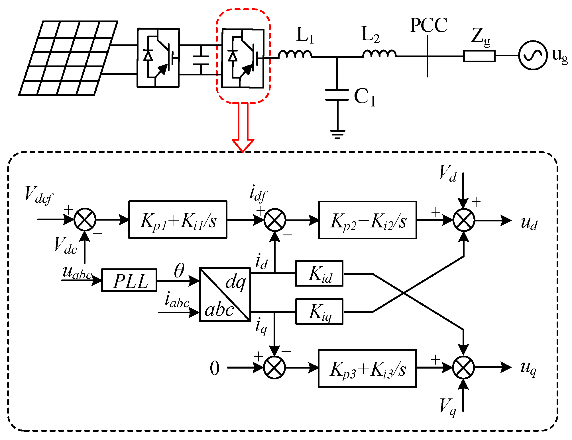
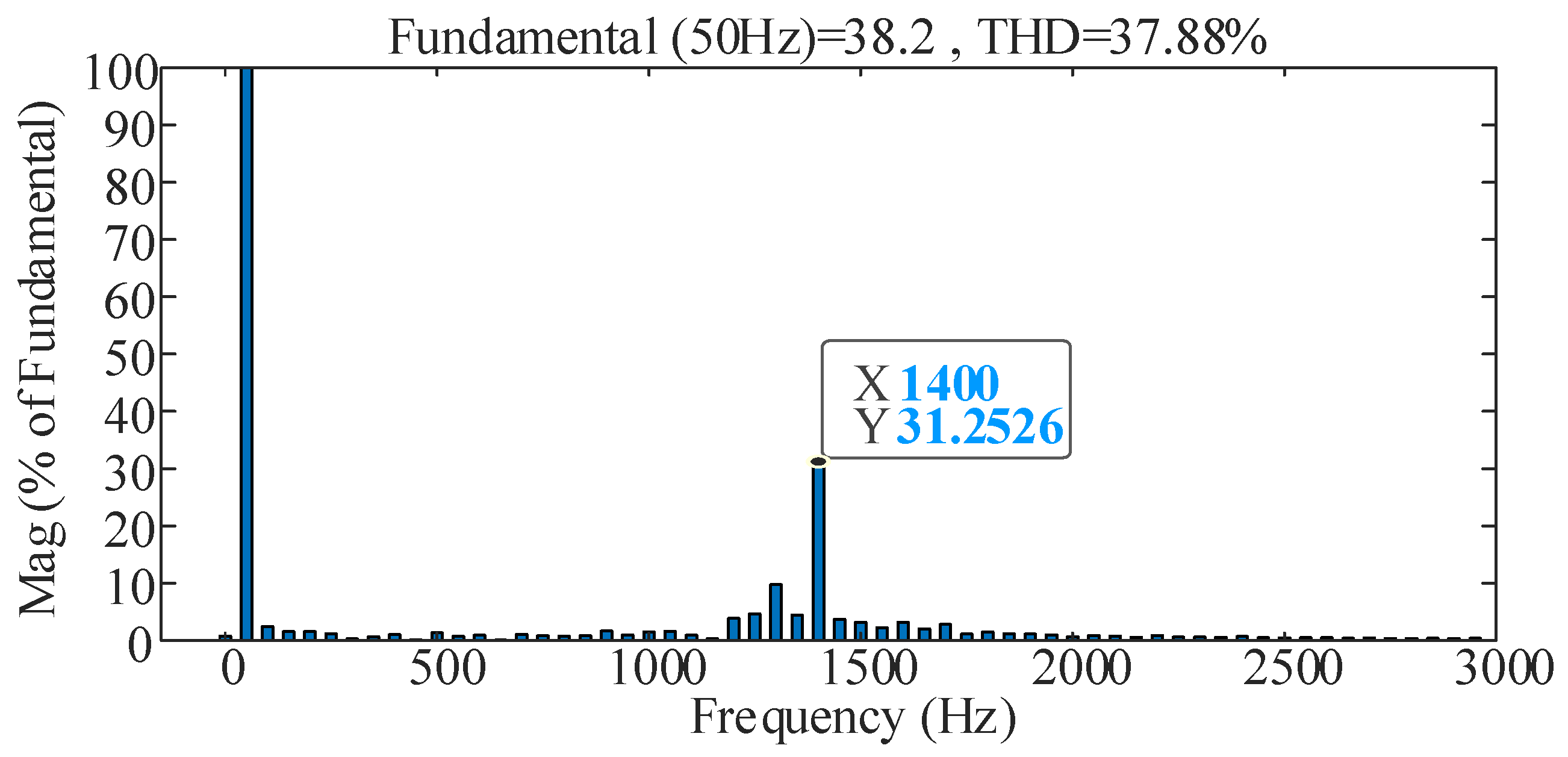
In the LCL-type PV grid-connected system, the PV inverter is connected to the grid through an LCL filter. The switching operation of the grid-connected inverter generates a wide range of harmonic components, which can be easily amplified near the main resonant frequency of the system and trigger resonance in the PV system. As shown in Figure 1, the photovoltaic array converts solar energy into electrical energy. The output direct current (DC) is boosted by the first converter to stabilize the DC capacitor voltage, and then converted into alternating current (AC) by the second inverter. The current is filtered by a filter structure with an inductor–capacitor–inductor (LCL) topology, and finally connected to the distribution network with a voltage of ug through a transmission line, where the internal grid impedance is denoted by Z_g. The detailed parameters of the PV generation system are provided in Appendix A. Under this specific operating condition, the system resonates at 1400 Hz, and this condition is defined as Resonance Scenario 1. The FFT (Fast Fourier Transform) analysis of the current at the PV grid connection point is presented in Appendix A.

(2) PV grid-connected system with SVG

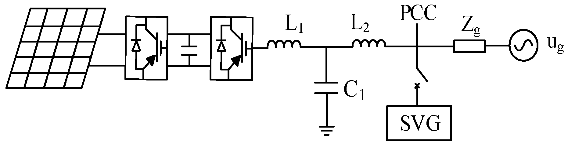
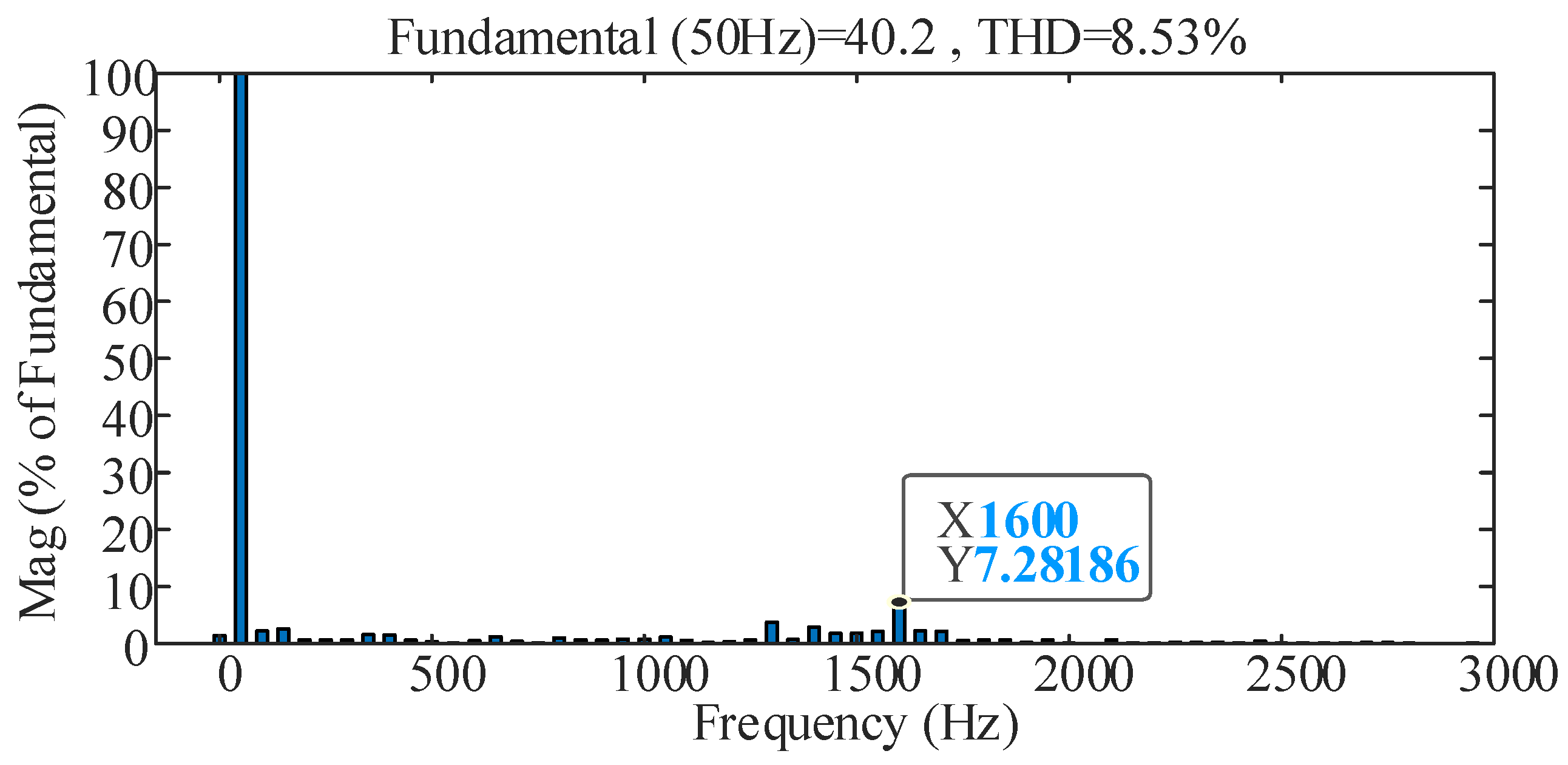
In PV grid-connected systems with SVGs, resonance is affected by multiple factors, including the LCL filter parameters, grid impedance, and the parameters of the SVG. When the grid impedance is high, grid-voltage phase locking may fail, and the voltage control loop of the compensation device may also become unstable. As a result, the compensation device may become inoperable, thereby triggering system resonance. In this case, the resonance is caused by abnormal operation of the compensation device. However, existing studies have mainly focused on resonance caused by harmonic amplification in the system. In contrast, the resonance investigated in this paper occurs when the SVG operates normally. It is caused by harmonic injection from both the SVG and the PV inverter, together with variations in the equivalent grid-side impedance. As shown in Figure 2, the SVG is connected in parallel at the grid connection point of the PV grid-connected power generation system. The system is connected to a distribution network with voltage u_g through a transmission line, and the internal grid impedance is denoted by Z_g. The parameters of the PV power generation system are provided in Appendix A. When line maintenance is carried out or the grid-connection line is extended, the grid-side equivalent inductance increases. When the grid-connection line inductance increases to L_g = 2.5 mH, the system resonates at 1600 Hz. This operating condition is defined as Resonance Scenario 2. The FFT analysis of the current at the PV grid connection point is also provided in Appendix A.

(3) Newly built PV grid-connected system with SVG

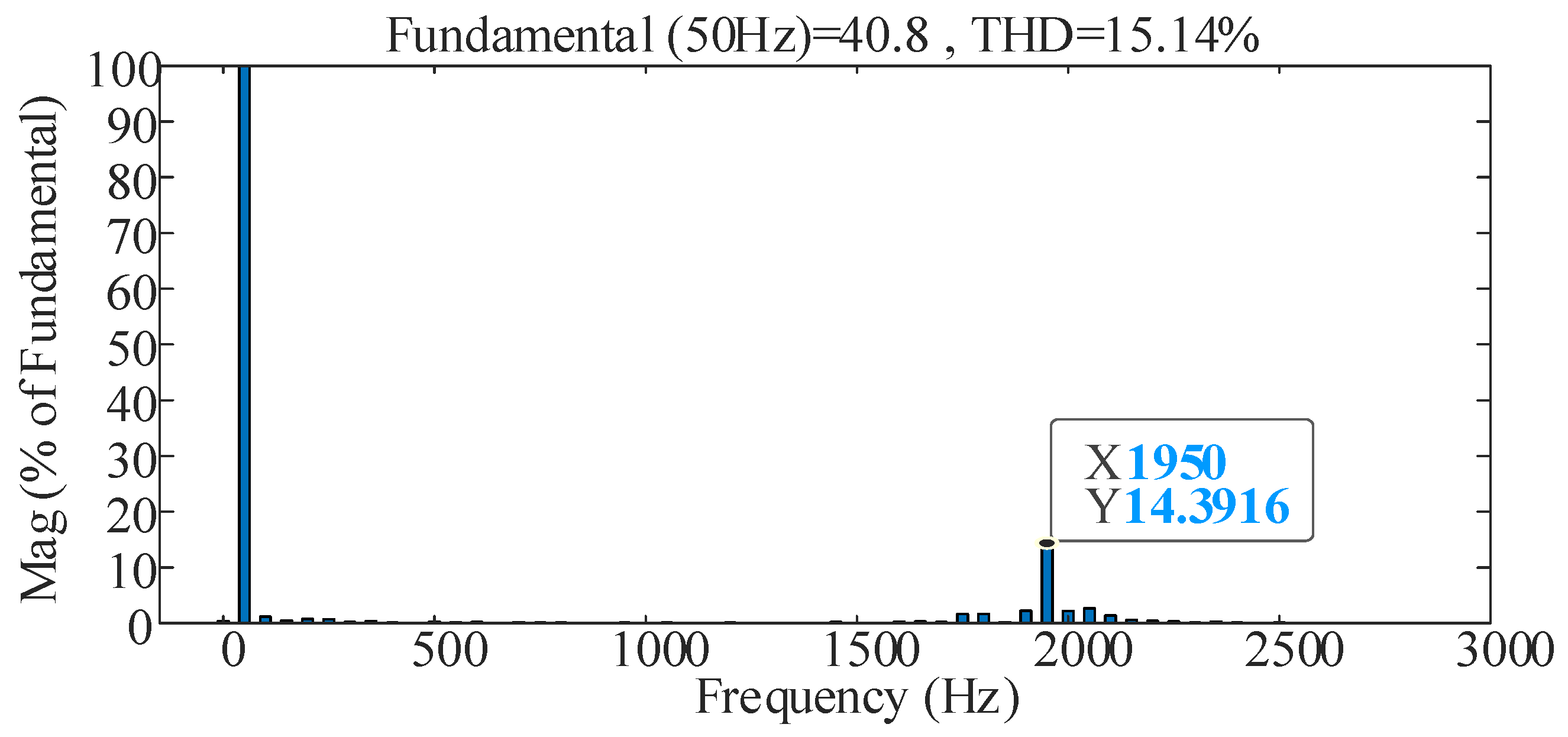
In a newly built PV grid-connected system equipped with SVG, parameter mismatches among the SVG, the PV system, and the grid-side equivalent impedance may cause resonance or even instability in the control loops of the inverter and the compensation device. As a result, the compensation device and the system form an oscillatory loop, which amplifies resonance at a specific frequency. As shown in Figure 2, the photovoltaic grid-connected system is connected in parallel with a newly commissioned SVG, and the system is connected to the 380 V distribution network through a transmission line, where the internal grid impedance is denoted as Z_g. The parameters of the photovoltaic grid-connected system are detailed in Appendix A. Due to improper selection of SVG and mismatched control parameters, the impedance of its output line and the proportional coefficient of the inner current loop are altered. When the SVG is connected at 0.2 s, the system resonates at 1950 Hz. This operating condition is defined as Resonance Scenario 3. The FFT analysis of the current at the PV grid connection point is also provided in Appendix A.

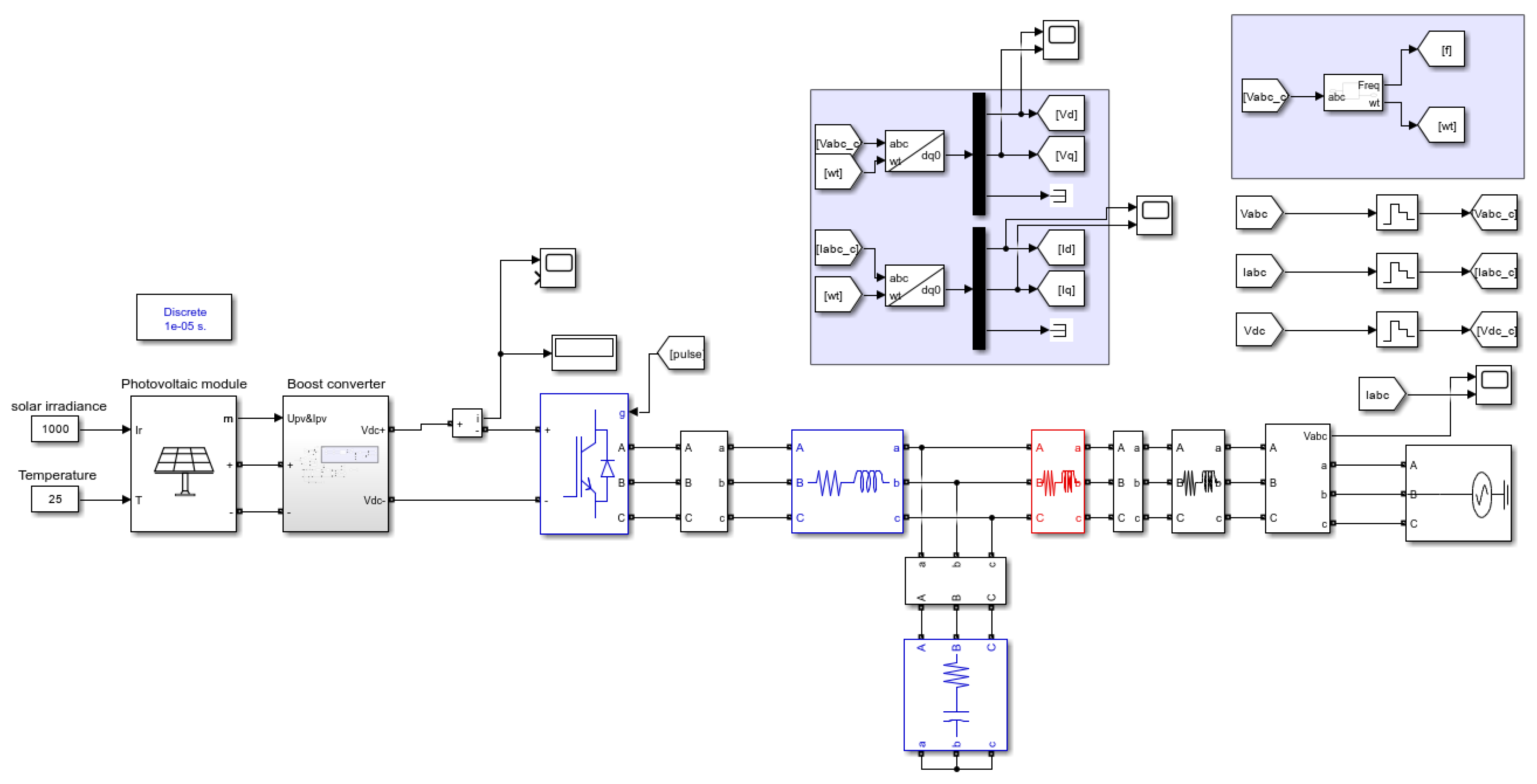
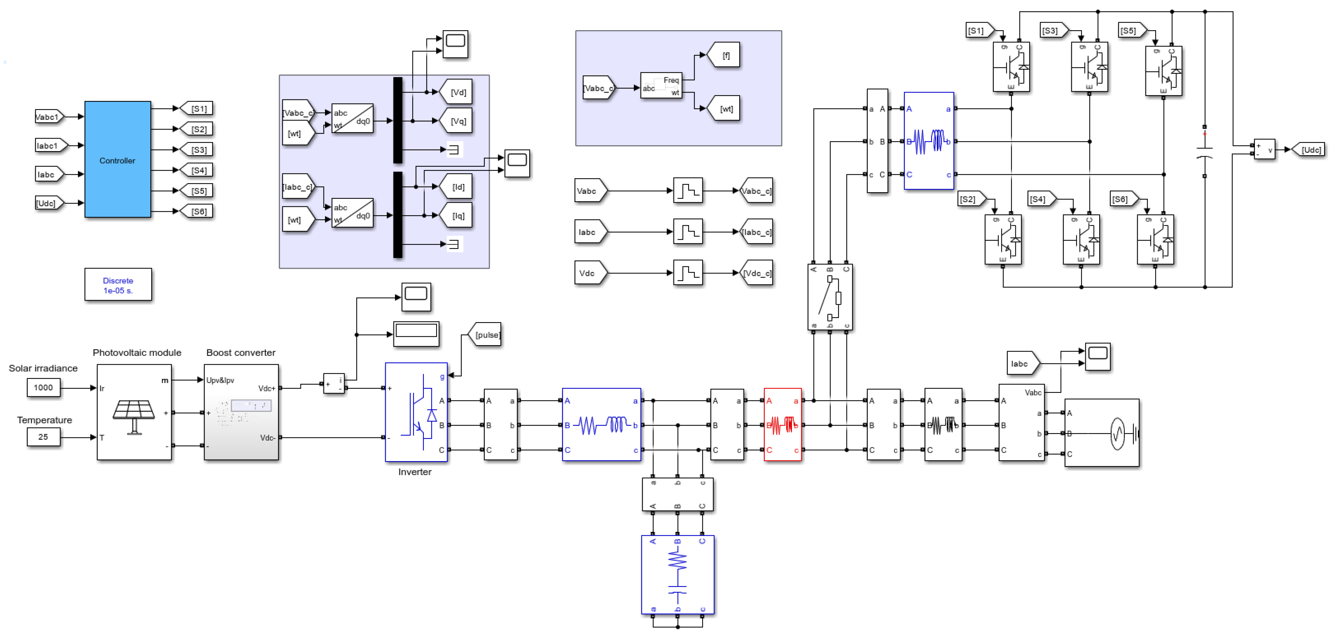
The operating resonant currents for the three cases above were derived from the resonance models built on the MATLAB/Simulink platform. These currents were analyzed by FFT using the powergui module. The FFT results and the simulation schematic diagrams are presented in Appendix A. The schematic diagrams for Scenario 2 and Scenario 3 are identical.

3. Resonance Suppression Strategies for PV Grid-Connected Systems

The impedance reshaping-based suppression strategy avoids the complex research on the resonance mechanism of photovoltaic systems and instead focuses on the impedance characteristics of the entire grid-connected system. By adjusting the frequency characteristics of the inverter output impedance or the equivalent grid-connected impedance, it eliminates the conditions for the occurrence of the main resonant peak in the system within the key frequency band, improves the phase margin and gain margin, thereby suppressing resonance and enhancing the dynamic stability of the system.

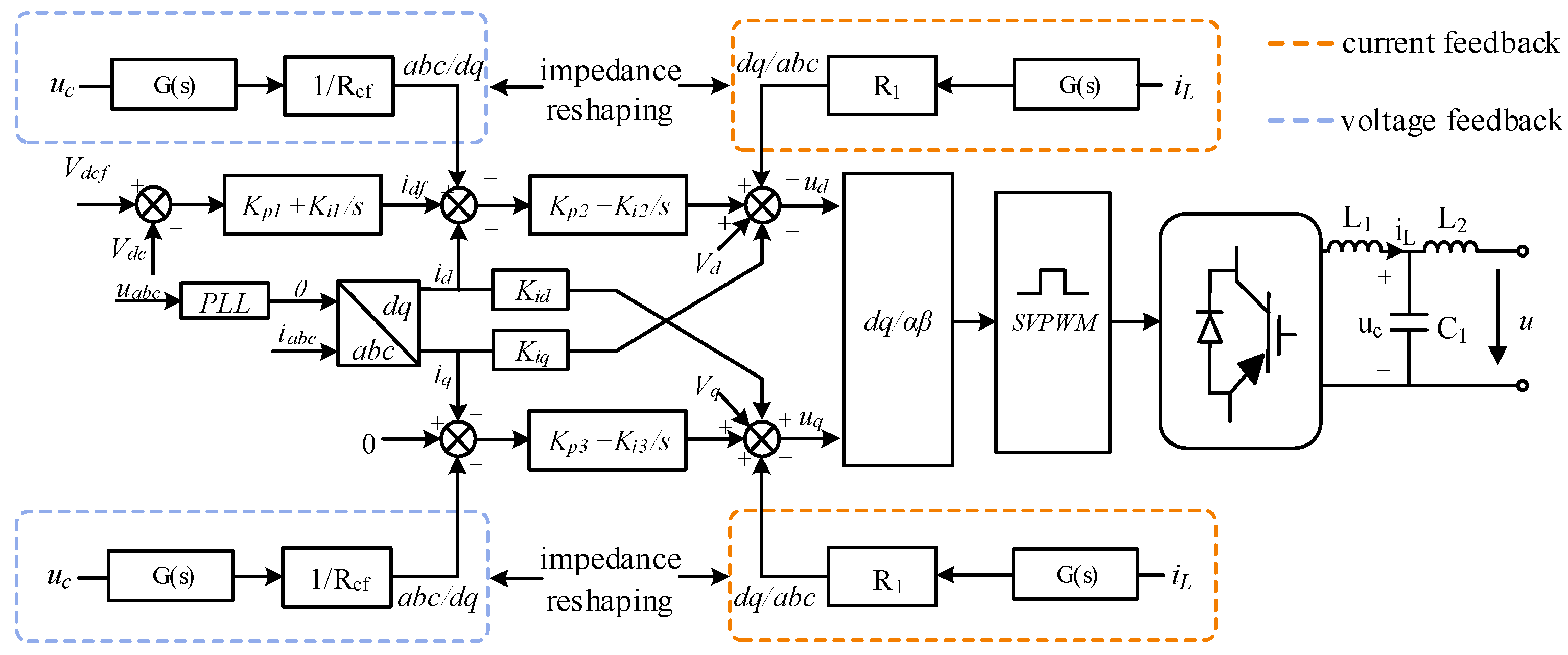
For resonance suppression in PV grid-connected systems, multiple impedance reshaping strategies are adopted in this study to improve the comparability and rationality of the experiments. As shown in Figure 3, the impedance reshaping resonance suppression strategy introduces additional virtual resistors R₁ and R_cf into the controlled source branch of the grid-connected inverter to regulate the voltage and current commands. These virtual resistors provide damping for harmonic resonances at different frequencies, thereby suppressing resonance. However, the direct introduction of virtual resistors also attenuates the power-frequency fundamental current component. According to the superposition theorem, the introduced virtual impedance only needs to function in frequency bands other than the power-frequency fundamental band. Therefore, two feedback functions are introduced in this paper to extract resonance components in frequency bands other than the power-frequency fundamental component. Their transfer functions are expressed as follows:

$$G_1(s)={\displaystyle \frac{2\zeta {\omega }_{1}s}{s^2+2\zeta {\omega }_{1}s+{{\omega }_1}^2}}$$

(1)

$$G_2(s)={\displaystyle \frac{s^2+{{\omega }_2}^2}{s^2+2\zeta {\omega }_{2}s+{{\omega }_2}^2}}$$

(2)

In the formula, ζ denotes the damping ratio, ω₁ represents the angular frequency at the main resonant frequency, and ω₂ represents the angular frequency at the power frequency.

Figure 3. Impedance reshaping suppression strategy for PV grid-connected systems.

Figure 3. Impedance reshaping suppression strategy for PV grid-connected systems.

In summary, based on the G₁/G₂ feedback functions, three impedance reshaping modes, namely single voltage feedback, single current feedback, and combined voltage-current feedback, are constructed, leading to a total of six resonance suppression strategies. These strategies serve as the experimental and control groups for subsequent verification of the correctness and effectiveness of the method proposed in this paper.

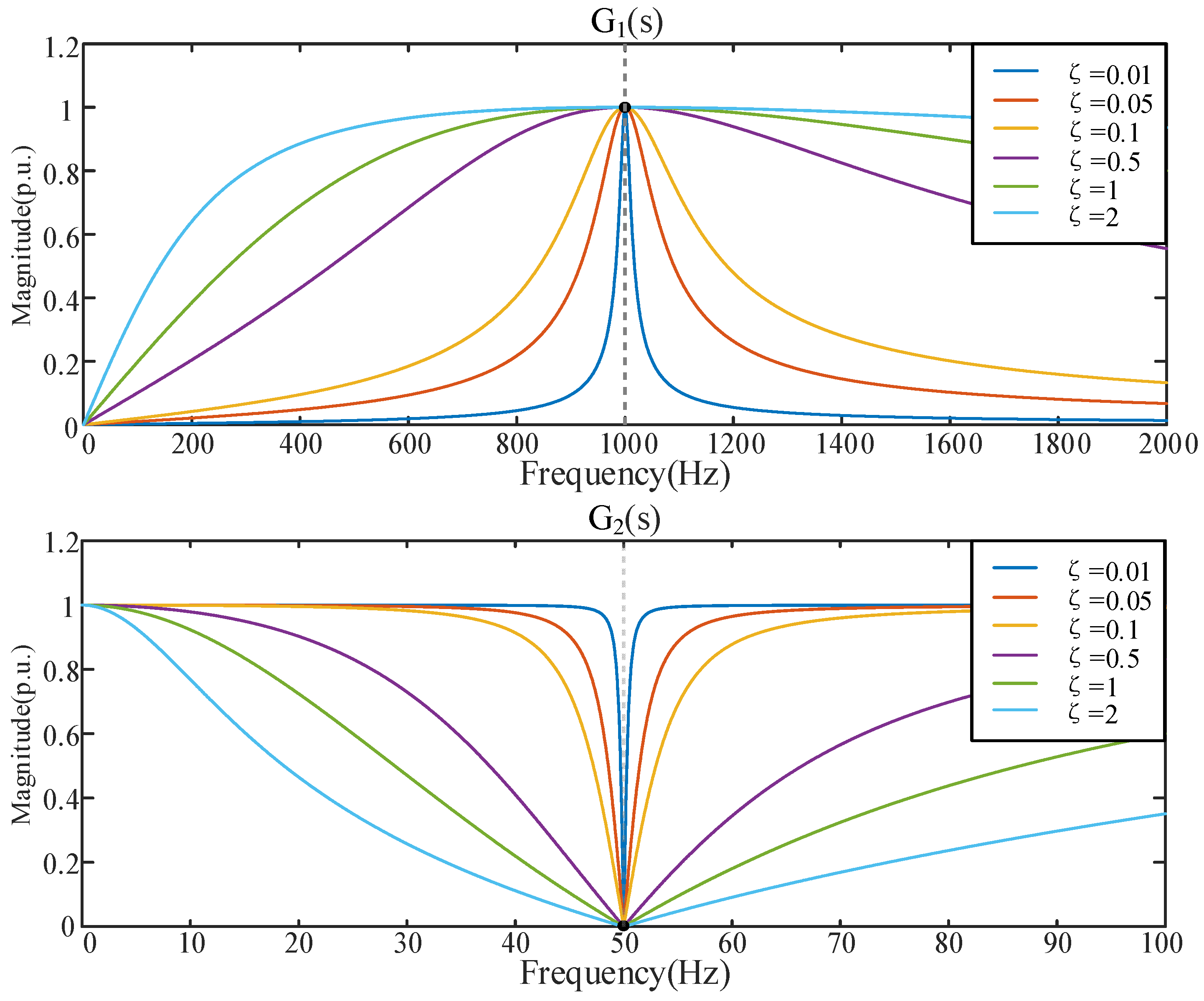
As shown in Figure 4, 1000 Hz and 50 Hz are set as the angular frequency calculation frequencies for G₁(s) and G₂(s) for illustrative analysis. For the two feedback functions (filters), the damping ratio ζ is a key parameter that determines the response speed, frequency selectivity, and stability. In engineering applications for resonance suppression, the underdamped design range of 0 < ζ < 1 is widely adopted. If ζ is too small, the filter exhibits overly strong frequency selectivity and a narrow bandwidth, leading to poor adaptability to resonance frequency shifts caused by grid impedance fluctuations and reduced stability. If ζ is too large, the filter has excessive damping and a slow response speed, resulting in an excessively slow resonance suppression rate, which hinders the subsequent evaluation of strategy differences. Therefore, after comprehensive consideration of the above factors, ζ = 0.5 is selected to balance the response speed, frequency selectivity, and stability. Based on the above analysis of resonance extraction and Figure 4, the two feedback functions should extract the resonant component while rejecting the power-frequency component. Thus, ω₁ represents the angular frequency at the main resonant frequency, and ω₂ represents the angular frequency at the power frequency. The value of virtual impedance is usually determined empirically; in this paper, it is set to R_cf = R₁ = 60 Ω.

4. Construction of the Evaluation System

4.1. Construction of Evaluation Indicators

Although some evaluations of suppression strategies have been reported in existing studies, they still show limitations in multi-scenario and multi-dimensional assessment. First, in the evaluation of a single suppression strategy, most studies only consider the overall THD variation and the settling time of the THD curve, while ignoring the attenuation characteristics of the main harmonic/resonance components. Moreover, the value standards of indicators vary across studies, resulting in a lack of accuracy and rigor. Second, in the comparison of suppression performance among multiple strategies, although THD is used as a quantitative indicator, key local indicators are neglected, including suppression speed, peak fluctuation of resonant current, and amplitude level of the main resonant component after suppression, leading to a single evaluation perspective.

To achieve a multidimensional quantitative evaluation of resonance suppression strategies for PV grid-connected systems, this study draws on the concepts of robustness evaluation in power systems, takes the dynamic response characteristics of the system into account, and constructs evaluation indicators from both local and global perspectives.

(1) Attenuation factor characteristic index α

During the resonance suppression process, the peak value of the main resonant current in each cycle usually decays in a manner similar to an exponential function. This behavior essentially reflects the dissipative effect of system damping on resonant energy. Therefore, in engineering practice, the least squares method can be used to fit an exponential function to the peak values of the main resonant current in each cycle [16,17]. The attenuation factor is a key parameter used to characterize the decay rate of the resonance amplitude of the system response [18]. A larger attenuation factor indicates a faster decay of the main resonant current component. Since the decay speed of the main resonant current is an important dimension for evaluating resonance suppression, the attenuation factor α is selected as the evaluation index.

Taking a second-order underdamped RLC (Resistor–Inductor–Capacitor) series resonant circuit as an example, the time-domain response of the main resonant current can be expressed as follows:

$$i(t)=I_0{e}^{-\alpha t}\sin ({\omega }_{0}0t+\varphi )$$

(3)

The time-domain expression of the peak fitting curve for the main resonant current is given as follows:

$$Y(t)=C_1{e}^{-\alpha t}+C_2$$

(4)

In the above equation, I₀ denotes the initial resonance amplitude; α denotes the attenuation factor, which characterizes the decay rate of the resonance amplitude of the system response; ω₀ denotes the damped resonance frequency; ϕ denotes the initial phase angle; C₁ denotes the initial peak current amplitude; and C₂ denotes the DC (direct current) component of the fitted curve.

(2) DC component index I_dc of the fitting curve

From the construction process of the attenuation factor characteristic index detailed above, the DC component index I_dc of the fitted curve is used to characterize the average amplitude level of the main resonant current after suppression. A higher average amplitude of the post-suppression main resonant current indicates a poorer suppression effect on this current component, while a lower average amplitude corresponds to more thorough resonance suppression. As the main resonant current is the most dominant component of the overall resonance, the DC component I_dc of the fitted curve can effectively quantify the performance of the suppression strategy on the most critical part of the resonance (i.e., the main resonant component), enabling rapid observation of the suppression state of the core resonant component. Since the fitted curve can accurately characterize the variation law of the system’s resonant current, a 5% threshold is adopted in engineering practice, which approximately corresponds to three time constants. At this threshold, the resonant power is extremely low, and its impact on the system can be neglected. Therefore, the moment when the exponential decay component of the fitted curve drops to 5% of its initial value is defined as the suppression end time.

(3) Steady-state peak variance index σ² of the main resonant current

Following the application of the resonance suppression strategy, a minor residual resonant component persists in the main resonant current. The variance metric is employed to quantify the fluctuation of the peak amplitude of the main resonant current post-suppression, which in turn characterizes the stability of this current component. Specifically, the peak variance of the post-suppression main resonant current has a negative correlation with its stability: a larger variance corresponds to poorer current stability. This fluctuation arises because variations in grid-side parameters and the inherent time-delay characteristics of the inverter introduce additional harmonics, which superimpose on the main resonant current and cause amplitude variations. Accordingly, the variance σ² of the post-suppression main resonant current amplitude can simultaneously reflect the suppression effect on both the main resonant component and other harmonics near the resonant frequency. A high variance indicates unstable main resonant current after suppression. Under this condition, the system is more prone to triggering new resonances when subjected to new excitation sources, such as grid fluctuations, load variations on the user side, or adjustments to the proportional coefficient of the control loop. Thus, the variance σ² of the post-suppression main resonant current amplitude is selected as one of the core evaluation indicators in this work.

The variance of the current peak value is expressed as follows:

$${\sigma }^2={\displaystyle \frac{1}{N}}{{\displaystyle {\sum }_{i=1}^N(i_{peak}-\mu )}}^2$$

(5)

In the above equation, N denotes the number of peak data points of the main resonant current; i_peak denotes the peak value of the main resonant current in each cycle; and μ denotes the mean value of the peak values of the main resonant current.

(4) Index of the total resonant current THD reduction rate η%

Total Harmonic Distortion (THD) is defined as the ratio of the total root-mean-square (RMS) value of all harmonic components in a signal to the RMS value of its fundamental component. It reflects the degree of deviation of all harmonics relative to the fundamental wave, and is usually expressed as a percentage. While most existing studies evaluate the performance of suppression strategies using the absolute variation of THD, this paper constructs the THD reduction rate η% before and after the implementation of suppression measures on this basis. The THD reduction rate η% can characterize the overall resonance suppression effect, covering both the main resonant current and other low-amplitude resonant currents. Therefore, the THD reduction rate η% is selected as a holistic evaluation indicator in this study. The THD reduction rate of the total resonant current can be expressed as follows:

$$\eta \%={\displaystyle \frac{TH{D}_{init}-TH{D}_f}{TH{D}_{init}}}\times 100\%$$

(6)

In the formula, THD_init denotes the THD of the total resonant current before suppression, and THD_f denotes the THD of the total resonant current after suppression.

Notably, the four aforementioned indicators are mutually independent. The damping factor α and the THD reduction rate η% are formulated from the perspectives of suppression speed and overall resonance suppression performance, respectively. Meanwhile, the DC component I_dc of the fitted curve characterizes the mitigation effect of the suppression strategy on the main resonant current, whereas the variance σ² of the current peak reflects the stability of the main resonant current upon the completion of the suppression process. Even when the main resonant current is suppressed to a high degree, the variance of the current peak may still remain at a high level, resulting in insufficient stability of the post-suppression current. Therefore, these four indicators are established from four dimensions: the suppression speed, suppression depth, and post-suppression stability of the main resonant current, as well as the overall suppression degree of the total resonant current. Together, they form a multi-dimensional evaluation system covering both transient and steady-state characteristics, as well as local and global performances.

(5) Comprehensive performance index Q_s of the suppression strategy

Based on the four characteristic indices constructed above, the evaluation result is obtained by linearly weighting each index. Since this indicator is derived from the aforementioned four indices and serves as a multi-dimensional performance metric for suppression strategies, Q_s is adopted as the quantitative indicator to evaluate the final suppression effect of the strategy. Its expression is as follows:

$$Q_s=K_1\alpha +K_2{I}_{dc}+K_3{\sigma }^2+K_4\eta \%$$

(7)

In the formula, K_i (i = 1, 2, 3, 4) denotes the weighting coefficient of each index. The comprehensive performance index constructed from the above four indices quantitatively characterizes the overall performance of different suppression strategies under different operating scenarios from both local and global perspectives.

(6) Robustness characteristic index R_s

Based on the construction process of the comprehensive performance index Q_s for the suppression strategy mentioned above, the comprehensive performance indices of a single suppression strategy under multiple scenarios are linearly weighted, and the resulting value is taken as the robustness index R_s. Since R_s is derived from the different performance indices Q_s of a single strategy under various scenarios, this indicator comprehensively considers the overall performance of a single strategy in multiple scenarios. Therefore, the robustness index R_s is selected as the indicator to quantify the adaptability of the suppression strategy, and its expression is as follows:

$$R_s={\lambda }_1{Q}_1+{\lambda }_2{Q}_2+{\lambda }_3{Q}_3$$

(8)

In the formula, Q_i (i = 1, 2, 3) denotes the comprehensive performance index of the suppression strategy under the three scenarios, and λ_i (i = 1, 2, 3) denotes the weighting coefficient of each index. The robustness index can quantitatively characterize the adaptability of a single suppression strategy under multiple scenarios, i.e., its comprehensive suppression effect in various scenarios. A larger value of R_s indicates better robustness, whereas a smaller value indicates poorer robustness.

4.2. Selection of the Evaluation Method

When multiple performance indicators are used to assess the comprehensive capability of an evaluation object, the choice of evaluation method is crucial. An appropriate evaluation method can provide an intuitive and accurate characterization of the overall performance of the evaluated object. Multi-indicator evaluation methods can generally be classified into subjective weighting methods and objective weighting methods [19].

Subjective weighting methods include the analytic hierarchy process, Delphi method, and expert scoring method. These methods determine indicator weights mainly based on expert experience or the subjective judgment of decision-makers, which may result in strong subjectivity and incomplete evaluation results in some cases. The single-core indicator subjective weighting method is a typical evaluation approach among subjective weighting methods. It selects the most important indicator based on experience and assigns a high weight to it, while indicators regarded as unimportant in subjective judgment are given low weights or even excluded from the evaluation. This method is widely adopted in existing studies on the evaluation of suppression strategies; for instance, the performance of a suppression strategy is often evaluated solely using the THD variation. Therefore, the single-core indicator subjective weighting method is chosen for comparison in this work.

The formula for calculating the evaluation results is as follows:

$$Q_{sub}=A_1\alpha +A_2{I}_{dc}+A_3{\sigma }^2+A_4\eta \%$$

(9)

In the formula, A_i (i = 1, 2, 3, 4) represent the weight of different indicators. The formula for the robustness evaluation result is given as follows:

$$R_{sub}=B_1{Q}_{sub1}+B_2{Q}_{sub2}+B_3{Q}_{sub3}$$

(10)

In the formula, Q_subi (i = 1, 2, 3) represent the performance evaluation indices under the three scenarios, B_i (i = 1, 2, 3) represent the weight of different indicators.

Objective weighting methods determine indicator weights according to the intrinsic characteristics of data. With their data-driven objectivity and high reproducibility, typical objective weighting methods include the entropy weight method, factor analysis, and the coefficient of variation method. Compared with other mainstream objective weighting methods, the entropy weight method shows much higher applicability in this study. Factor analysis is centered on dimensionality reduction to extract common factors, and the abstract dimensionality-reduced indicators tend to obscure the physical connotation of the original indicator design. This means only the final evaluation result can be acquired, while the contribution of individual indicator differences to the result cannot be effectively analyzed. The coefficient of variation method assigns weights solely based on data dispersion, which easily overlooks the information differences between indicators, eventually leading to weight imbalance, and its weighting process lacks a clear physical meaning. In contrast, the entropy weight method is based on information entropy theory, with weights assigned according to the information content of original indicators, and has a well-defined physical meaning [20,21,22]. It also presents strong robustness to indicator data fluctuations and high evaluation accuracy in multi-scenario and multi-strategy assessment. In summary, for the resonance scenarios of grid-connected PV systems, the relevant indicators are constructed based on explicit physical connotation and feature strong objectivity. Therefore, the entropy weight method, among all objective weighting methods, is selected in this paper to evaluate the performance of resonance suppression strategies.

4.3. Entropy Weight Method

The entropy weight method is based on the relationship between information entropy and the degree of variation in indicators. Information entropy reflects the level of disorder or randomness in a system. In data-driven evaluation, a lower entropy value for a given indicator indicates a greater degree of variation among its data values, that is, a higher degree of dispersion. This implies that the indicator contains more useful information and should therefore be assigned a larger weight in the evaluation. The specific procedure is as follows:

(1) Data Standardization

Suppose there are m samples and n evaluation indicators, forming the original data matrix X = (x_ij)_m×n, i = 1, 2, …, m; j = 1, 2, …, n. Since indicators differ in their dimensional characteristics or are entirely dimensionless, standardization is essential to unify the data to the same order of magnitude and scale. Regarding positive indicators, higher values denote better performance, while for negative indicators, elevated values indicate inferior performance. The standardization formulas for positive and negative indicators are as follows:

$${x_{ij}}^{*}={\displaystyle \frac{x_{ij}-\min \left.\left\{x_{1j},\dots x_{nj}\right.\right\}}{\max \left.\left\{x_{1j},\dots x_{nj}\right.\right\}-\min \left.\left\{x_{1j},\dots x_{nj}\right.\right\}}}$$

(11)

$${x_{ij}}^{*}={\displaystyle \frac{\max \left.\left\{x_{1j},\dots x_{nj}\right.\right\}-x_{ij}}{\max \left.\left\{x_{1j},\dots x_{nj}\right.\right\}-\min \left.\left\{x_{1j},\dots x_{nj}\right.\right\}}}$$

(12)

(2) Calculate the information entropy of the indicators

The information entropy reflects the degree of information disorder of the indicator. The lower the information entropy is, the more important the indicator is. The formula is as follows.

$$E_j=-\ln {\left(n\right)}^{-1}{\displaystyle \sum _{i=1}^n{p}_{ij}}\ln \left(p_{ij}\right)$$

(13)

In the formula, $p_{ij}={x_{ij}}^{*}/{\displaystyle {\sum }_{i=1}^n{x_{ij}}^{*}}$, it represents the proportion of the standardized value of the i-th sample under the j-th indicator to the total sum of all samples under that same indicator. When p_ij = 0, take the limit value of $p_{ij}\ln \left(p_{ij}\right)$ as 0. E_j represents the information entropy value, which is used for further calculation of indicator weights, and its value ranges from 0 to 1.

(3) Calculate the entropy weight of the indicators

The weight of each indicator w_j represents the degree of influence of the indicator on the evaluation result, and the calculation formula is shown in Equation (14).

$$w_j={\displaystyle \frac{1-E_j}{{\displaystyle \sum _{j=1}^m\left(1-E_j\right)}}},{\displaystyle \sum _{j=1}^m\left(w_j\right)=1}$$

(14)

(4) Calculate the evaluation result

Following the calculation of each indicator’s weight using the entropy weight method, the assessment result of the evaluated object is derived by the formula given below.

$$S_i={\displaystyle \sum _{j=1}^m{w}_j{p}_{ij}}$$

(15)

In the formula, S_i stands for the comprehensive score of the i-th assessed object; w_j signifies the entropy weight of the j-th indicator, while p_ij denotes the value of the j-th indicator belonging to the i-th evaluation object after undergoing standardization.

Notably, the four evaluation indicators constructed above correspond to the four indicators (n = 4) in the m × n original data matrix used in the entropy weight method. Meanwhile, the six resonance suppression strategies presented in this study correspond to the six evaluation objects (m = 6) in the same matrix. By incorporating the evaluation procedure of the entropy weight method presented in Section 2, the comprehensive performance evaluation results (Q_s) of different strategies under different scenarios can be obtained. The calculation of K₁–K₄ follows the indicator weighting procedure of the entropy weight method (Equations (13) and (14)).

The evaluation of the robustness index Rs follows the same principle. Specifically, the comprehensive performance values Q_s of each suppression strategy under the three resonance scenarios constitute the three evaluation indicators (n = 3) in a new m × n matrix, while the six suppression strategies serve as the six evaluation objects (m = 6). The calculation of λ₁–λ₃ also follows the indicator weighting procedure of the entropy weight method (Equations (13) and (14)).

5. Example Analysis

In this chapter, the parameters of the suppression strategies were first adjusted under the same strategy and resonance scenario based on the four performance indices established in the preceding section. The validity of the proposed performance indices was then verified by examining the correspondence between their variation trends and the actual operating conditions of the system.

Subsequently, for the three resonance scenarios, the comprehensive performance and robustness of multiple suppression strategies were quantitatively evaluated by combining the established indices with the entropy weight method. The results indicate that Strategies 1, 2, 4, and 5 all exhibit different degrees of insufficient suppression effectiveness and limited robustness. These findings provide a theoretical basis for the development of resonance suppression strategies with adaptive parameter control capability. All the figures in the following case studies are drawn using MATLAB and Visio software.

5.1. Verification of Performance Indicators

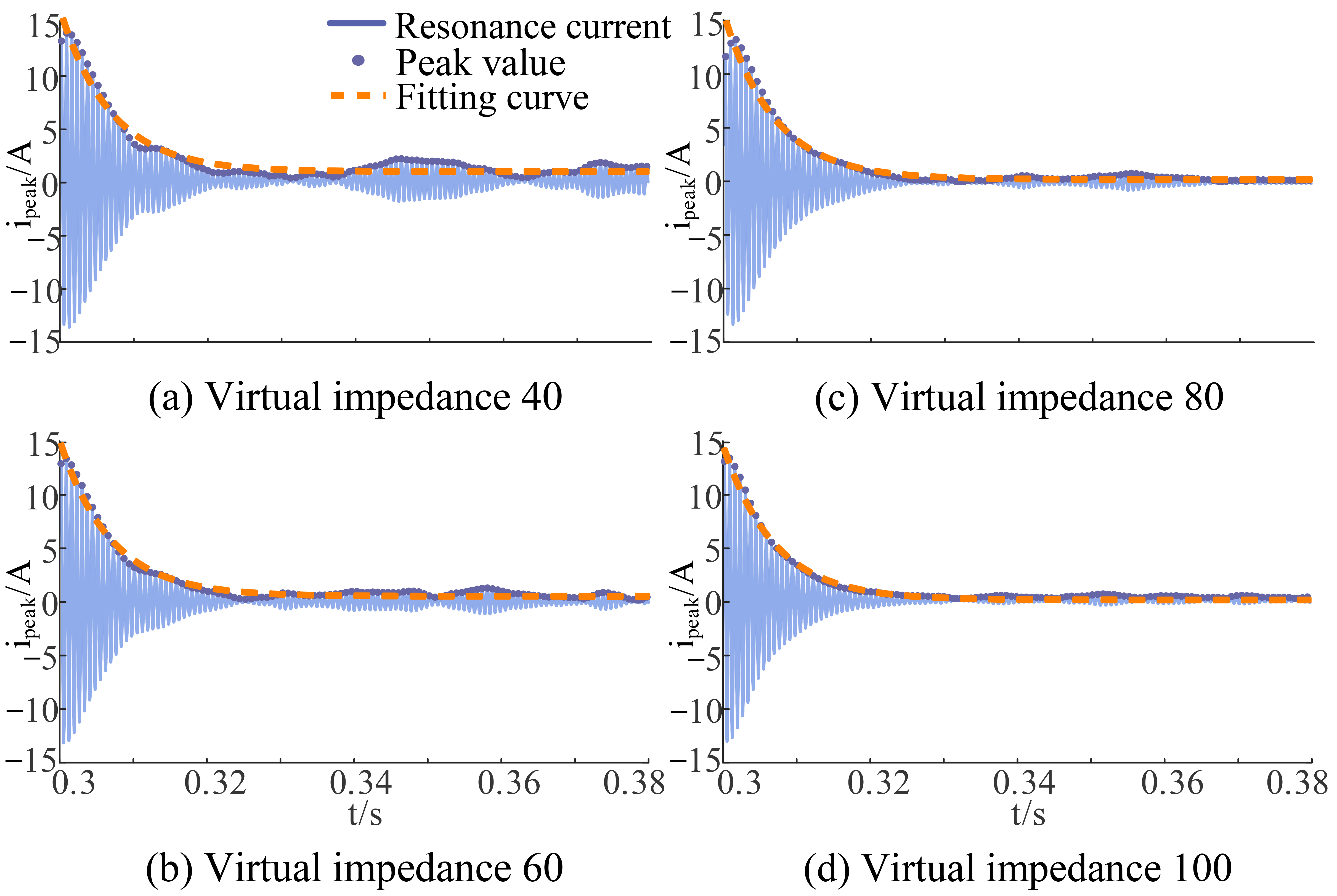
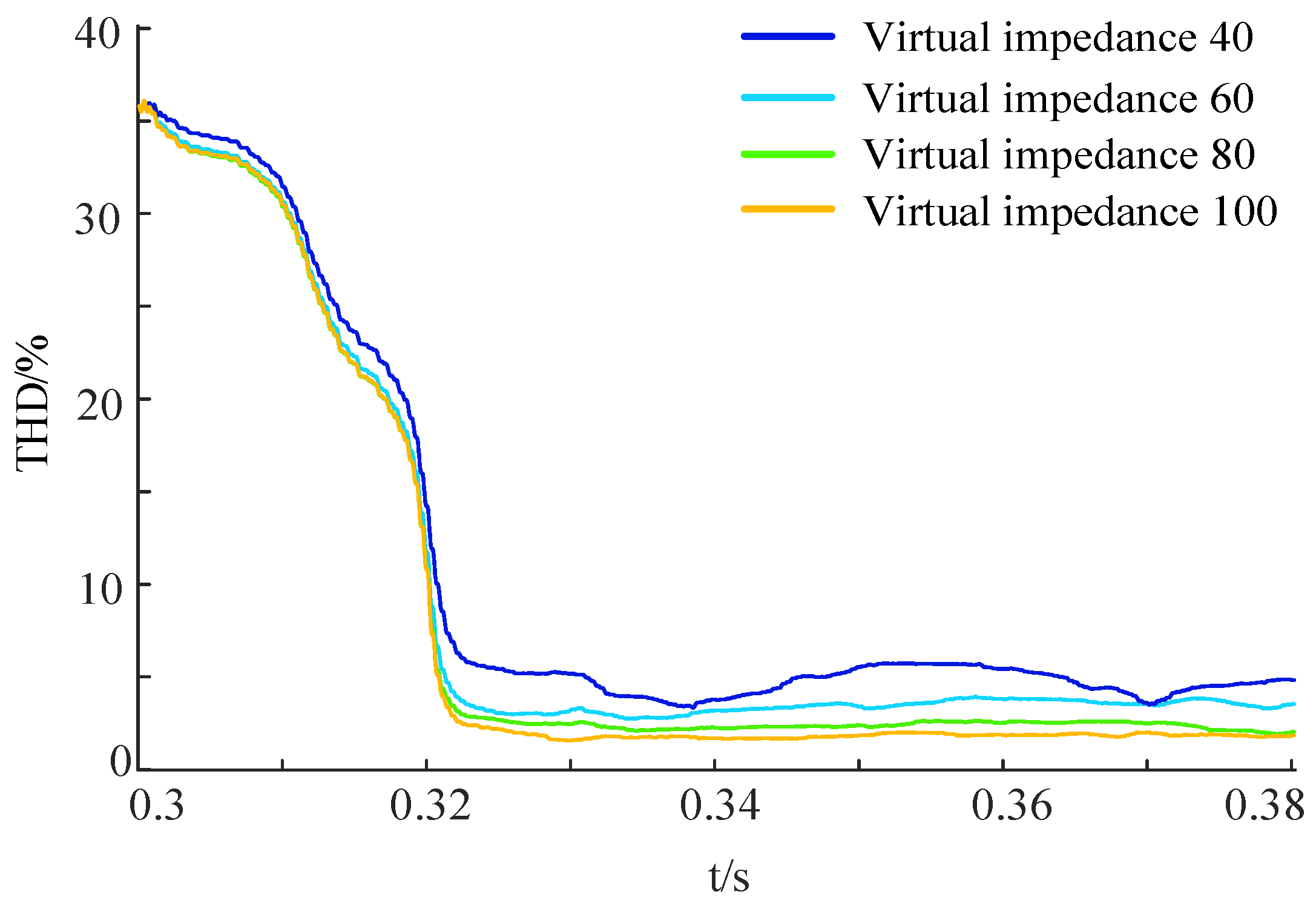
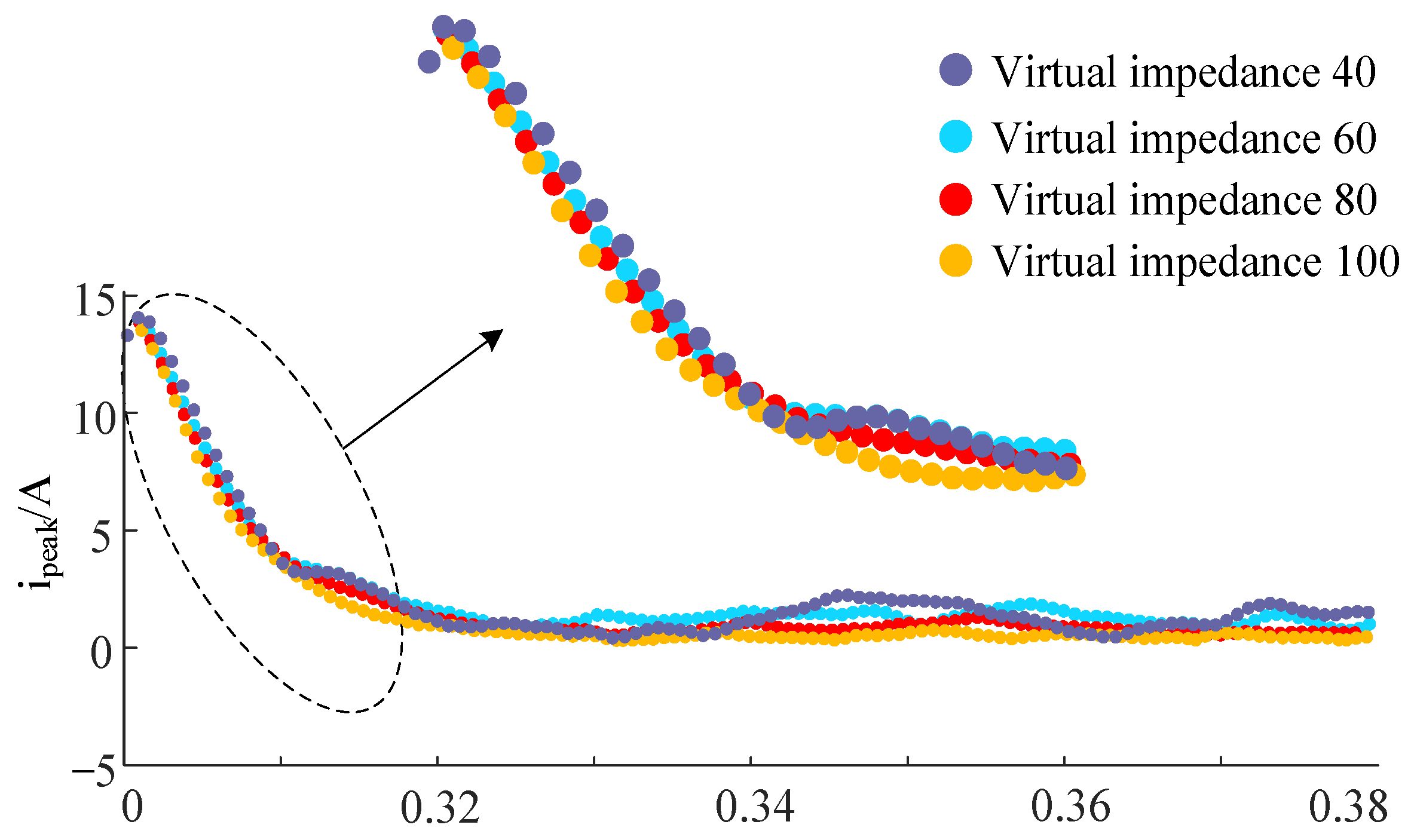
In the same LCL-type PV grid-connected system, with all other system parameters kept constant, the virtual impedance of Suppression Strategy 1 under the underdamped condition was set to 40, 60, 80, and 100 Ω, respectively, and the strategy was activated at 0.3 s. The resonance suppression effects on the 1400 Hz resonance peak under the four parameter settings were obtained. The fitted curves of the current amplitude at the resonance peak are shown in Figure 5, and the THD values under different parameter settings are presented in Figure 6. The raw index data and weighted index data for different virtual impedance values are provided in

Table 1. Original index data under different working conditions.

Virtual Impedance	α	η%	σ2	Idc
40	152.4515	86.5	0.2618	0.8721
60	152.9092	90.49	0.0688	0.5204
80	154.782	93.79	0.0358	0.1825
100	157.1128	94.57	0.0193	0.1288

and

Table 2. Weighted evaluation index data.

Virtual Impedance	α	η%	σ2	Idc	Qs
40	0	0	0	0	0
60	0.0362	0.1073	0.1537	0.1045	0.4017
80	0.1845	0.1961	0.18	0.2049	0.7655
100	0.369	0.217	0.1931	0.2209	1

, respectively.

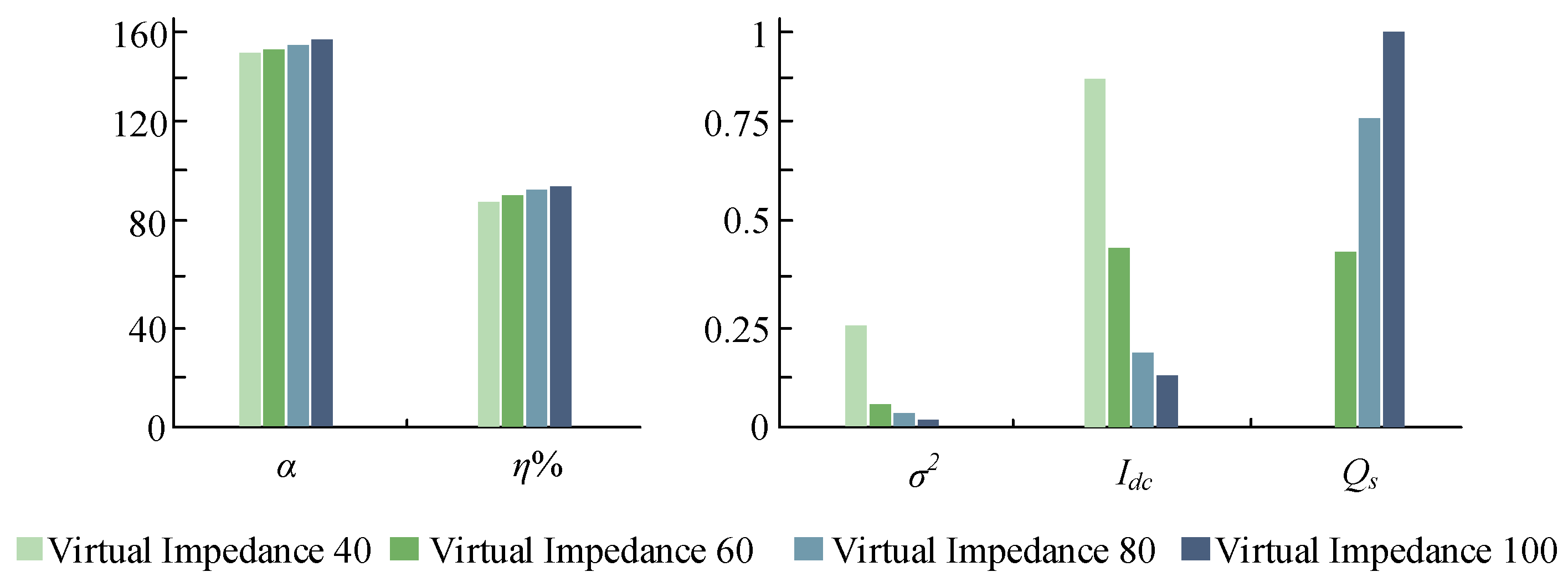
Based on the comprehensive analysis of Figure 5, Figure 6, Figure 7 and Figure 8, as virtual impedance increases, the variation trends of the four constructed indicators are consistent with those of the corresponding experimental performance indicators. The attenuation factor α is positively correlated with the decay rate of the main resonant current, while the THD reduction rate is positively correlated with the measured reduction in THD. The variance σ² of the steady-state main resonant current peak is negatively correlated with the fluctuation of the main resonant current after suppression, and the DC component index I_dc of the fitted curve is negatively correlated with the average amplitude level. In addition, when the virtual impedance is set to 100 Ω under underdamped operating conditions, the corresponding performance evaluation results are optimal. These results accurately reflect the actual operating characteristics of the system, thereby verifying the validity and reasonableness of the established performance indicators.

5.2. Evaluation of the Comprehensive Performance and Robustness of the Strategy

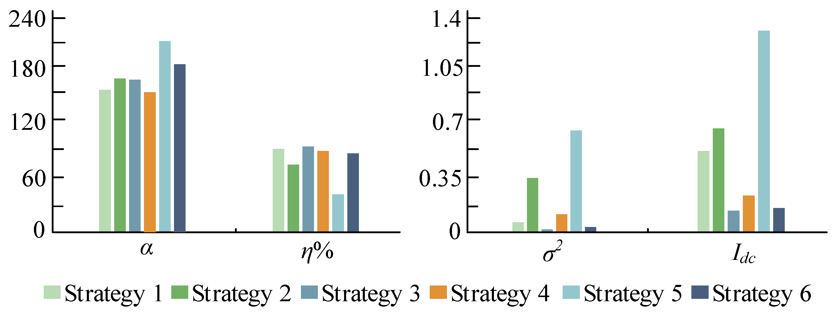
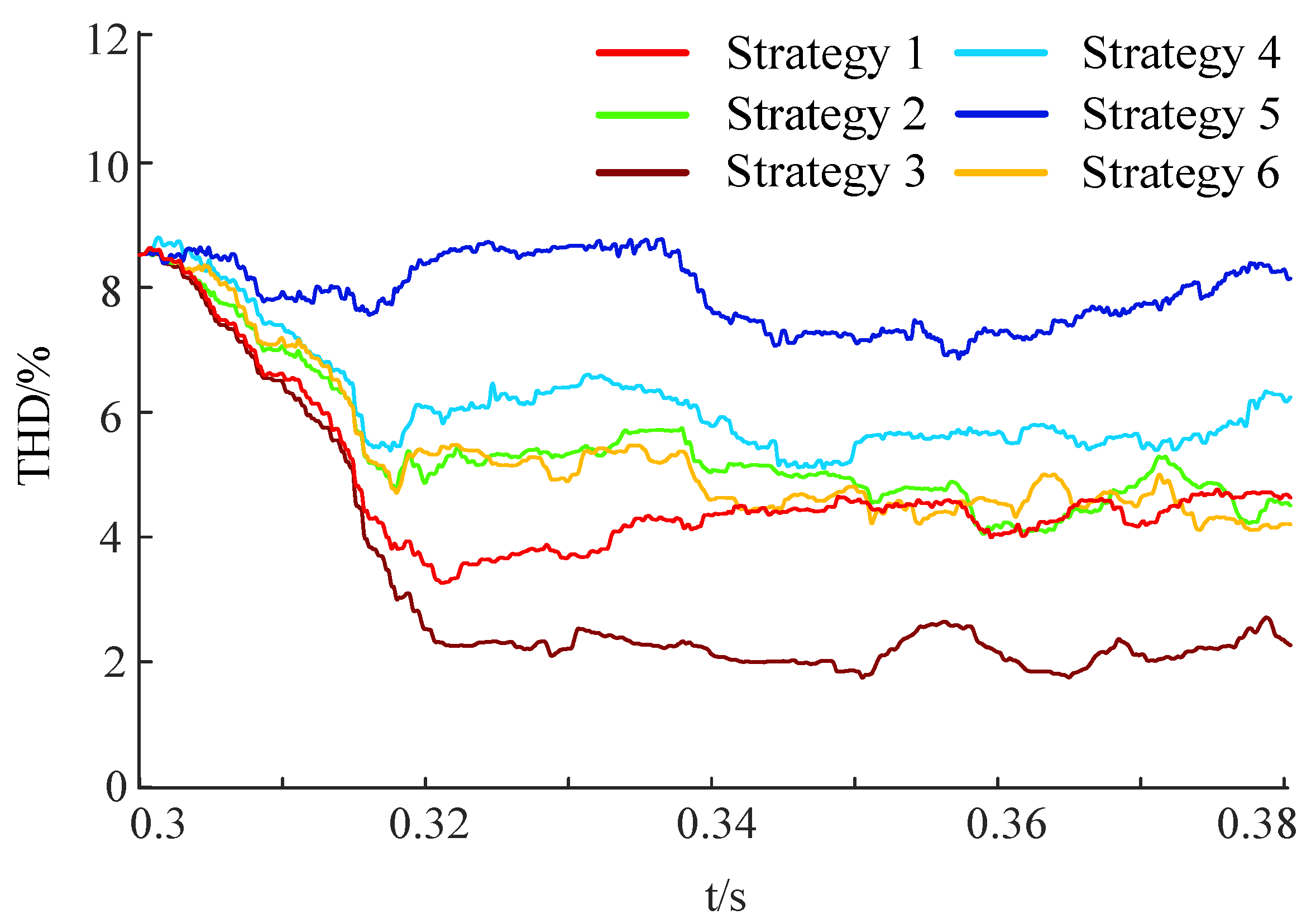
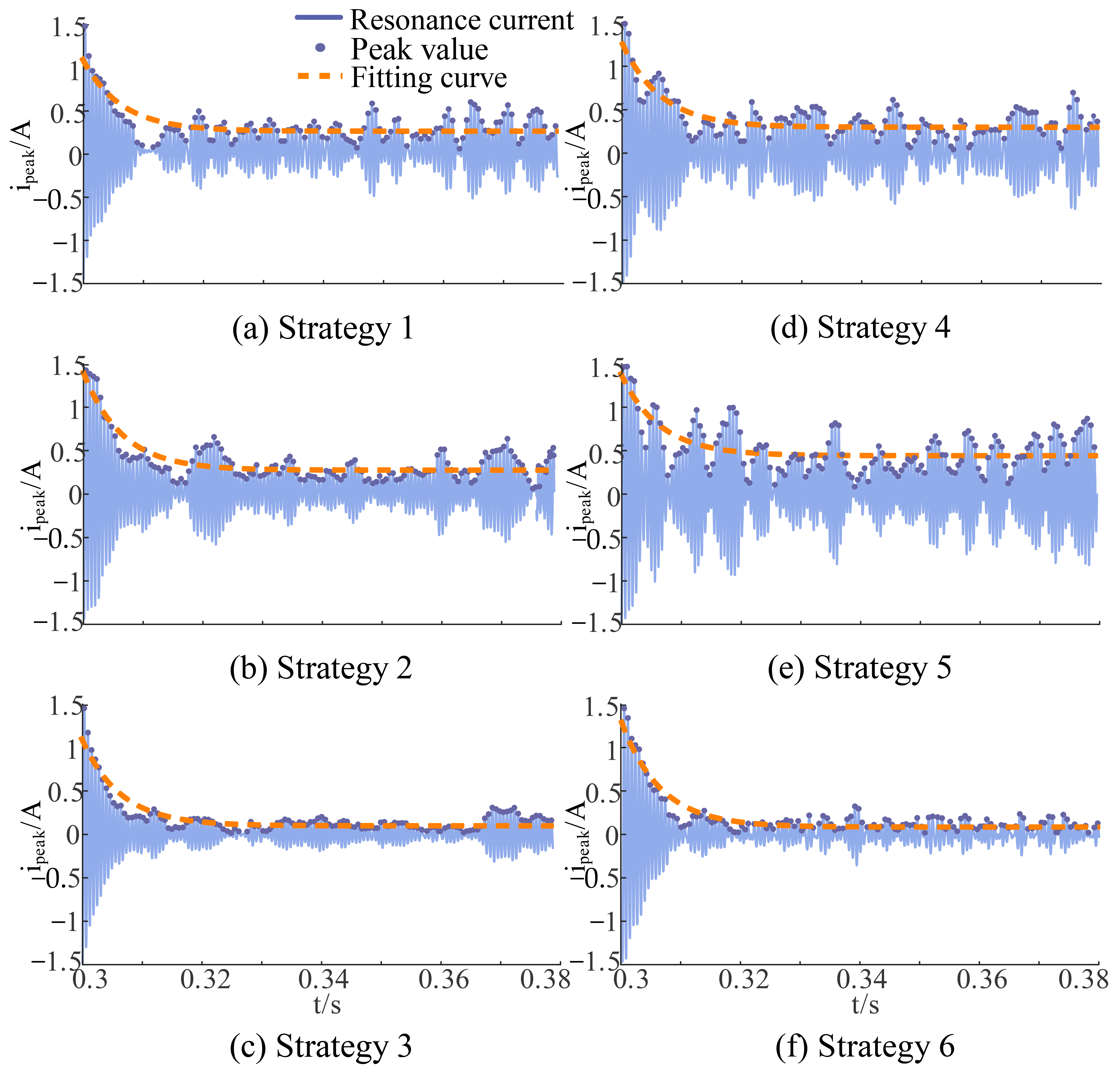
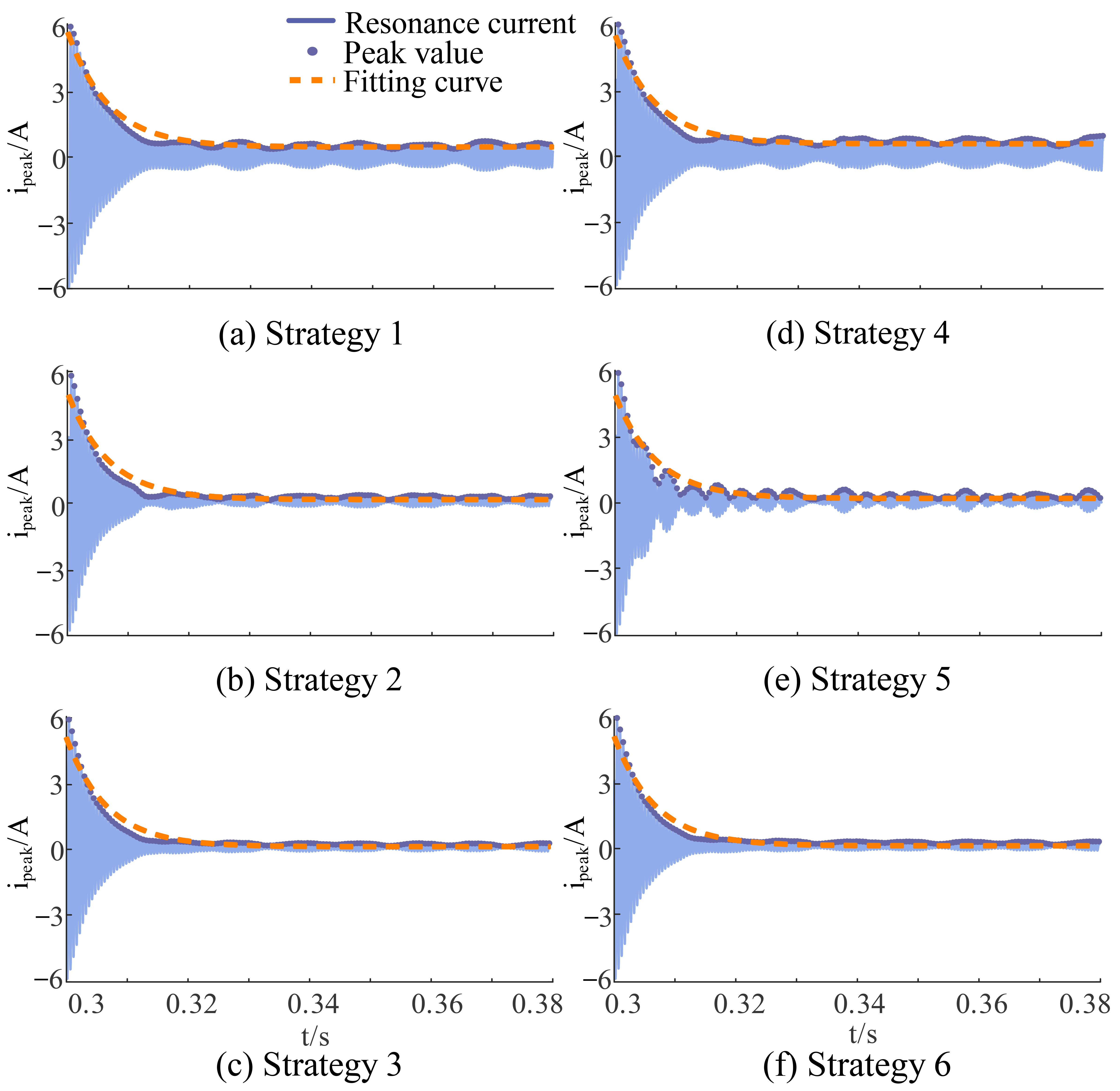
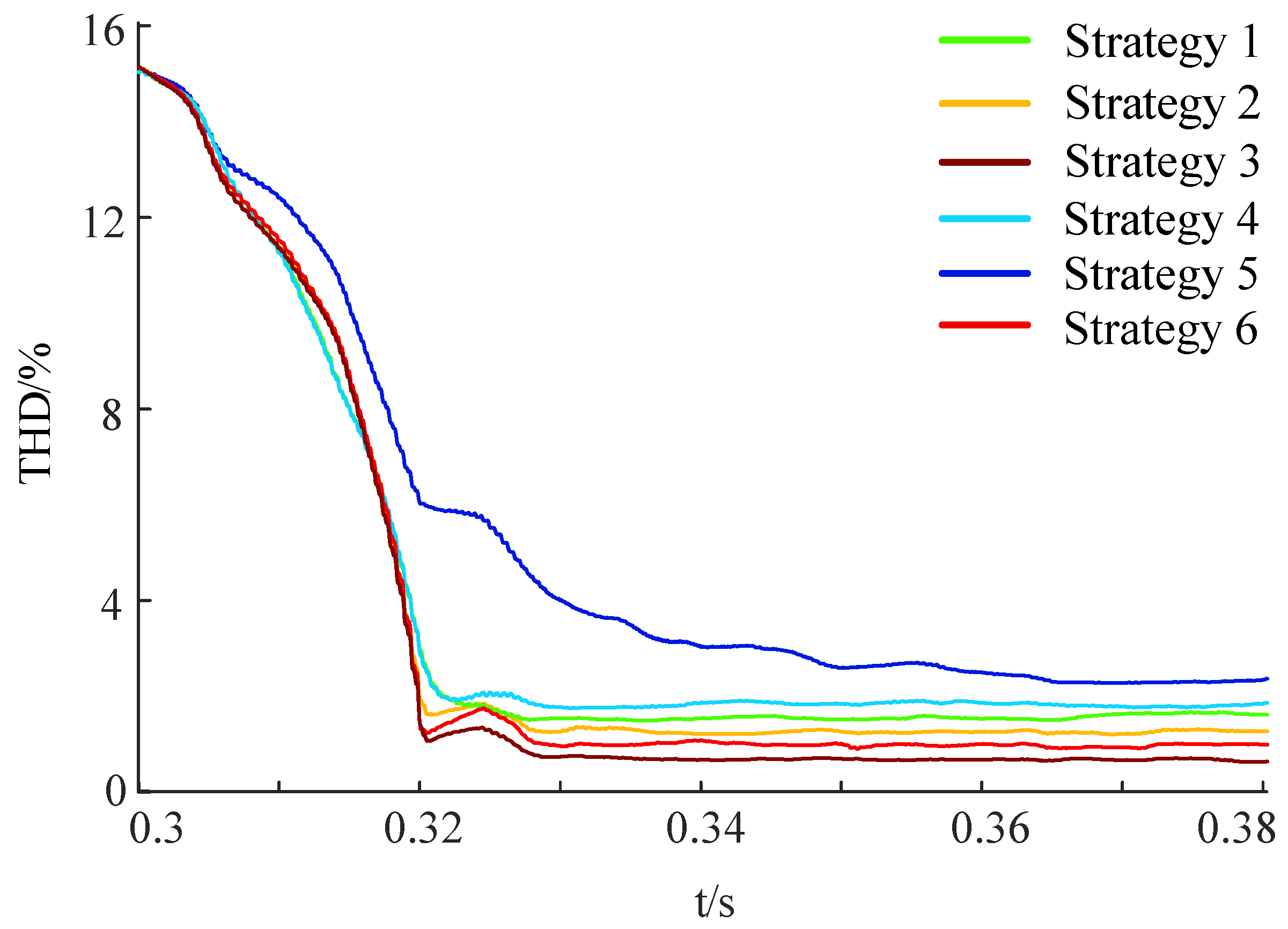
Using the MATLAB/Simulink platform, the resonance scenarios of the three PV grid-connected systems described in Section 2 were established, denoted as Scenarios 1, 2, and 3, respectively. The comprehensive performance and robustness of the six resonance suppression strategies under these three scenarios were quantitatively evaluated. The fitted curves of the main resonant current, the THD curves, and the original performance index data for the three resonance scenarios are shown in the following figures, while the weighted performance index data are provided in Appendix A.

(1) LCL-type PV grid-connected system

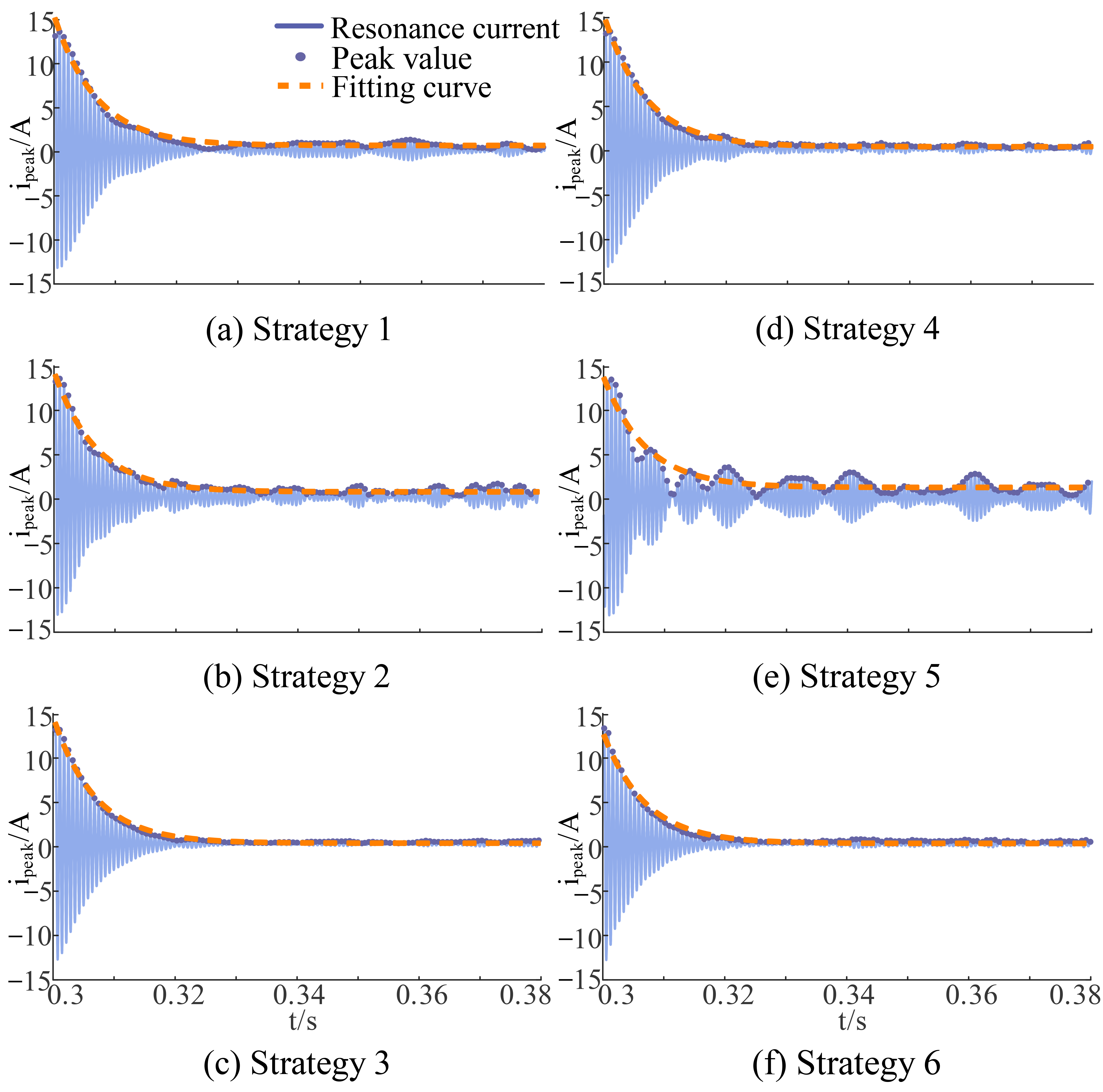
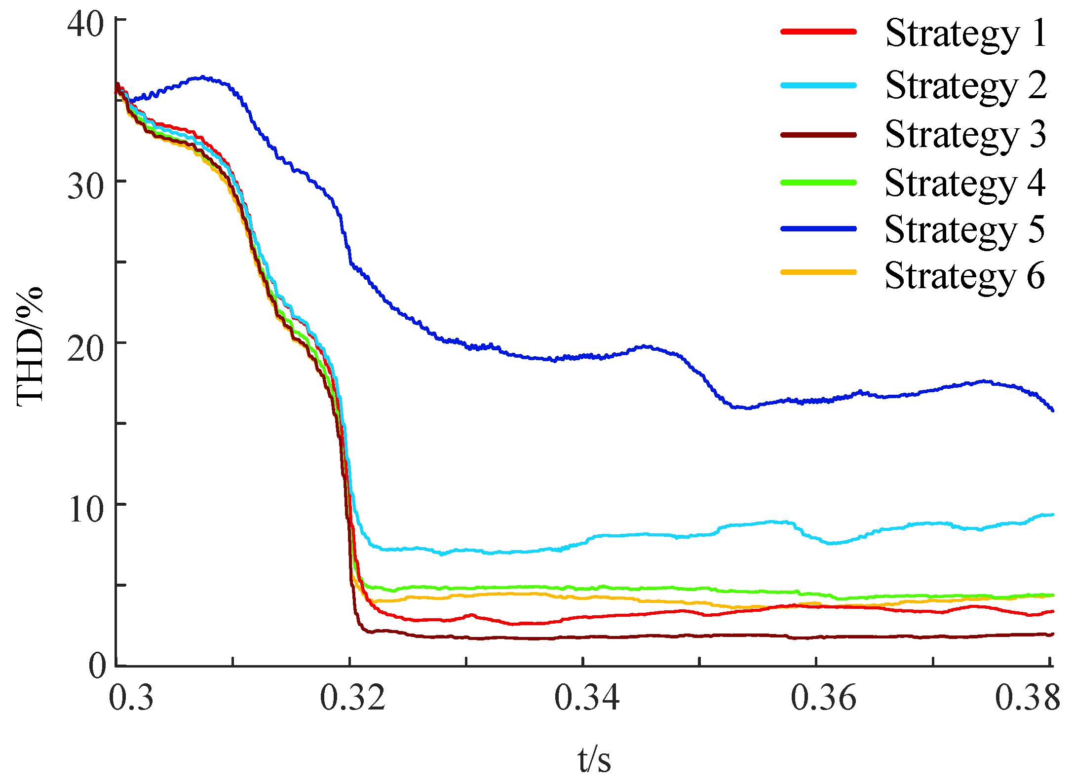
Scenario 1 corresponds to the first topology described in Section 2 (Figure 1). Resonance may be triggered upon grid connection, resulting in significant amplification of current harmonics at the grid connection point, an excessive THD level, and insufficient damping. The resonance attenuates slowly and may even exhibit a divergent trend. This scenario is common in medium- and low-voltage weak distribution networks, particularly in industrial areas with stringent power quality requirements. The main resonant current and its fitting curve are shown in Figure 9, and the THD curve is shown in Figure 10.

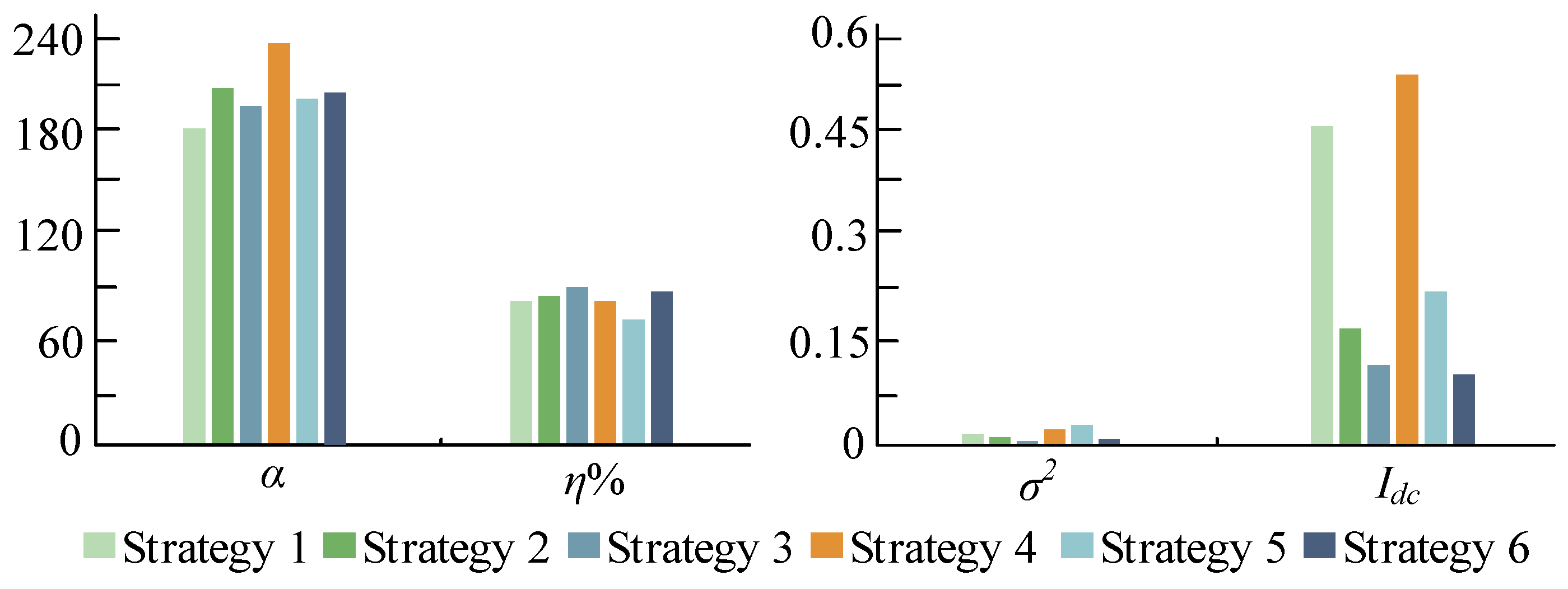
According to Figure 11 and

Table 3. Original index data of different strategies.

	α	η%	σ2	Idc
Strategy 1	152.9092	90.49	0.0688	0.5204
Strategy 2	164.4584	76.72	0.3453	0.6468
Strategy 3	162.4453	93.93	0.0125	0.1222
Strategy 4	150.9915	86.9	0.0440	0.2500
Strategy 5	212.7431	45.33	0.6317	1.3128
Strategy 6	184.0892	86.59	0.0207	0.1731

, in Scenario 1, Strategy 5 has the largest attenuation factor α. Strategy 3 shows the highest THD reduction rate η%, while the DC component of the fitted curve I_dc and the variance σ² of the steady-state main resonant current peak are the smallest.

(2) PV grid-connected system with SVG

Scenario 2 corresponds to the second topology described in Section 2 (Figure 2). Such systems can dynamically regulate reactive power output and absorption according to real-time grid operating conditions. When the voltage at the grid connection point deviates from the normal range, the SVG can respond rapidly to restore it to the allowable range. Combined with the LCL filter topology, the system can further reduce the total harmonic distortion (THD) of the grid-connected current and mitigate the risk of resonance. Resonance may occur immediately upon grid connection and exhibits characteristics such as multi-mode behavior, strong coupling, and high sensitivity to operating conditions. In addition to the inherent medium- and high-frequency resonance of LCL-type grid-connected systems, such systems also face potential resonance risks induced by the dynamic control of the SVG. The THD curve is shown in Figure 12, and the main resonant current with its fitting curve is shown in Figure 13.

According to the bar chart of the original performance indicators shown in Figure 14 and the original index data listed in

Table 4. Original index data under different working conditions.

	α	η%	σ2	Idc
Strategy 1	360.4523	48.18	0.0166	0.2428
Strategy 2	267.9423	41.03	0.0279	0.2436
Strategy 3	314.4973	69.87	0.0051	0.1236
Strategy 4	229.0664	31.65	0.0206	0.3099
Strategy 5	252.8377	8.39	0.0538	0.4453
Strategy 6	254.3310	43.26	0.0049	0.1057

, in Scenario 2, Strategy 1 has the largest attenuation factor α. Strategy 3 has the highest THD reduction rate η%, while Strategy 6 has the smallest variance of the peak value of the main resonant current after suppression σ² and the smallest DC component of the fitted curve I_dc.

(3) Newly built PV grid-connected system with SVG

Scenario 3 corresponds to the third topology described in Section 2 (Figure 2). Owing to insufficient parameter matching and inadequate coordinated commissioning, parameter mismatches may exist among the inverter, LCL filter, SVG, and grid impedance. This type of resonance mainly occurs at key operating nodes during the initial commissioning stage of the system, rather than during stable operation. At the moment of the first switching on or off of the reactive power compensator, or during the reactive power regulation process, the control parameters may not yet be optimized for on-site operating conditions. As a result, the response speed and regulation amplitude of the device may fail to adapt to real-time changes in system impedance, leading to reactive power regulation imbalance and triggering resonance. This resonance is characterized by multi-frequency-band superposition and strong suddenness, and it often occurs without obvious precursors when operating conditions change. Therefore, it poses significant challenges to the initial grid-connection commissioning and stable operation of newly built systems. The main resonant current and its fitting curve are shown in Figure 15, and the THD curve is shown in Figure 16.

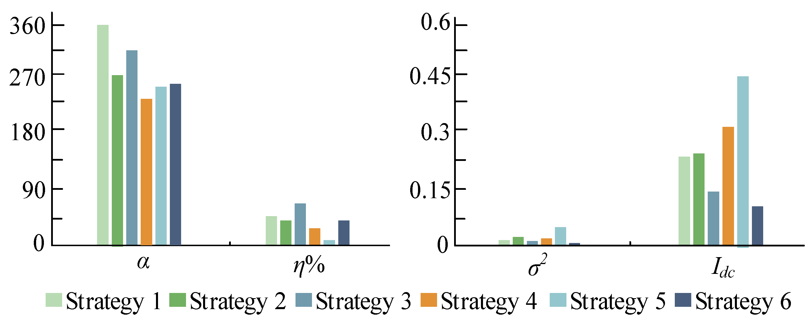
As shown in the bar chart of the original performance indicators in Figure 17, in Scenario 3, Strategy 4 has the largest attenuation factor α, Strategy 3 achieves the highest THD reduction rate η% with the smallest variance σ² of the suppressed current peak, and Strategy 6 has the smallest DC component I_dc of the fitted curve.

From the above analysis of the THD curves, the fitted curves of the main resonant current peak, the original index data (

Table 5. Original index data under different working conditions.

	α	η%	σ2	Idc
Strategy 1	180.8212	84.87	0.0108	0.4642
Strategy 2	207.0880	85.54	0.0083	0.1733
Strategy 3	197.2526	89.17	0.0059	0.1193
Strategy 4	235.4451	84.15	0.0128	0.5429
Strategy 5	200.8102	73.58	0.0274	0.2184
Strategy 6	203.9014	87.25	0.0074	0.1034

), and the bar chart of the original performance indicators, the trends of the indicators for different suppression strategies under different scenarios are not entirely consistent. Moreover, the magnitudes of the indicator data correspond well to the actual operating conditions, which further verifies the correctness of the constructed indicators.

(4) Comprehensive Performance and Robustness Evaluation Results

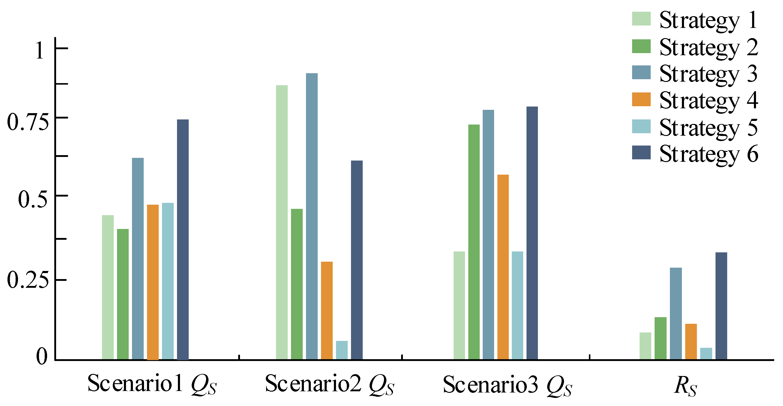
Based on the comprehensive performance results obtained for the three aforementioned scenarios, the entropy weight method was further adopted to calculate the robustness results of the six suppression strategies, with the comprehensive performance results serving as the evaluation indicators. Finally, the comprehensive performance and robustness of all suppression strategies were analyzed in an integrated manner.

From the case analysis, combined with the indicator data listed in Figure 18 and

Table 6. Performance and robustness evaluation results of all strategies under the three scenarios.

	Scenario 1 QS	Scenario 2 QS	Scenario 3 QS	RS
Strategy 1	0.4493	0.7896	0.3543	0.1011
Strategy 2	0.3925	0.4568	0.728	0.1263
Strategy 3	0.61	0.8573	0.7802	0.2846
Strategy 4	0.4694	0.2997	0.5714	0.1148
Strategy 5	0.4788	0.0675	0.3304	0.0433
Strategy 6	0.7432	0.6052	0.7887	0.3299

, the four indicators constructed in this paper—the attenuation factor α, the total resonant current THD reduction rate, the steady-state peak variance σ² of the main resonant current, and the DC component index I_dc of the fitting curve—do not exhibit completely consistent trends when different suppression strategies are applied under different scenarios.

In addition, different strategies show significant performance differences in each scenario. Under Scenario 1, the strategies are ranked in descending order of performance as follows: Strategy 6, Strategy 3, Strategy 5, Strategy 4, Strategy 1, and Strategy 2. According to the earlier construction analysis of the suppression strategies, among the six strategies, Strategies 3 and 6 adopt combined feedback. Compared with strategies using single feedback, their feedback paths contain more resonant components, resulting in better suppression performance. The first three strategies employ a band-pass filter as the feedback function, and the latter three adopt a notch filter. As shown in Figure 4 and Figure A1, since the notch filter can fully extract the main resonant components, while the band-pass filter exhibits inherent gain attenuation, Strategy 6 outperforms Strategy 3, and both strategies are generally superior to the remaining four strategies. Meanwhile, Strategies 4 and 5 comprehensively outperform Strategies 1 and 2.

Under Scenario 2, the ranking is: Strategy 3, Strategy 1, Strategy 6, Strategy 2, Strategy 4, and Strategy 5. Analyzed in conjunction with Figure A2: Strategies using the band-pass filter have a narrower passband than those using the notch filter, and thus show stronger targeting for the 1600 Hz main resonant component. In contrast, strategies using the notch filter extract other harmonics introduced by the SVG and the grid side, which weakens the resonance suppression effect. Therefore, Strategy 3 outperforms Strategy 6, and Strategies 4 and 5 exhibit better overall performance than Strategies 1 and 2. Meanwhile, the capacitor voltage is less affected by grid impedance variations. Therefore, combined with the advantage of the feedback function G₁(s), the performance of Strategy 1 is even better than that of Strategy 6.

Under Scenario 3, the ranking is: Strategy 6, Strategy 3, Strategy 2, Strategy 4, Strategy 1, and Strategy 5. As shown in Figure A3, the spectral distribution of Scenario 3 is similar to that of Scenario 1. Combined with the analysis of Scenario 1, Strategy 6 also outperforms Strategy 3 and Strategy 4 outperforms Strategy 1. However, unlike Scenario 1, the proportional gains of both the PV inverter and the SVG are increased in Scenario 3, which introduces additional phase lag in the control loops. Meanwhile, the resonant peak frequency rises to 1950 Hz; with identical parameter settings, the notch filter exhibits a more pronounced phase lag at the resonant peak compared with the band-pass filter. This ultimately results in a loss of system phase margin and reduced equivalent damping. Accordingly, the performance of Strategy 5, which adopts the notch filter, deteriorates drastically, ranking it below Strategy 2 with the band-pass filter.

Among the above strategies, Strategy 6 ranks second only under Scenario 2 and is the optimal strategy in all other scenarios, so Strategy 6 inevitably shows the strongest robustness. From the case results, the ranking of the strategies in terms of universality (i.e., adaptability) across the three scenarios is: Strategy 6, Strategy 3, Strategy 2, Strategy 4, Strategy 1, and Strategy 5.

Based on the above comprehensive analysis of the suppression strategies and case study results, the evaluation results of performance and robustness are consistent with the performance ranking trend of the suppression strategies, which further verifies the accuracy of the evaluation method proposed in this paper.

5.3. Comparison with the Subjective Weighting Method

In this section, the advantages and evaluation accuracy of the entropy weight method (the evaluation method adopted in this paper) were verified by comparing it with the subjective weighting method.

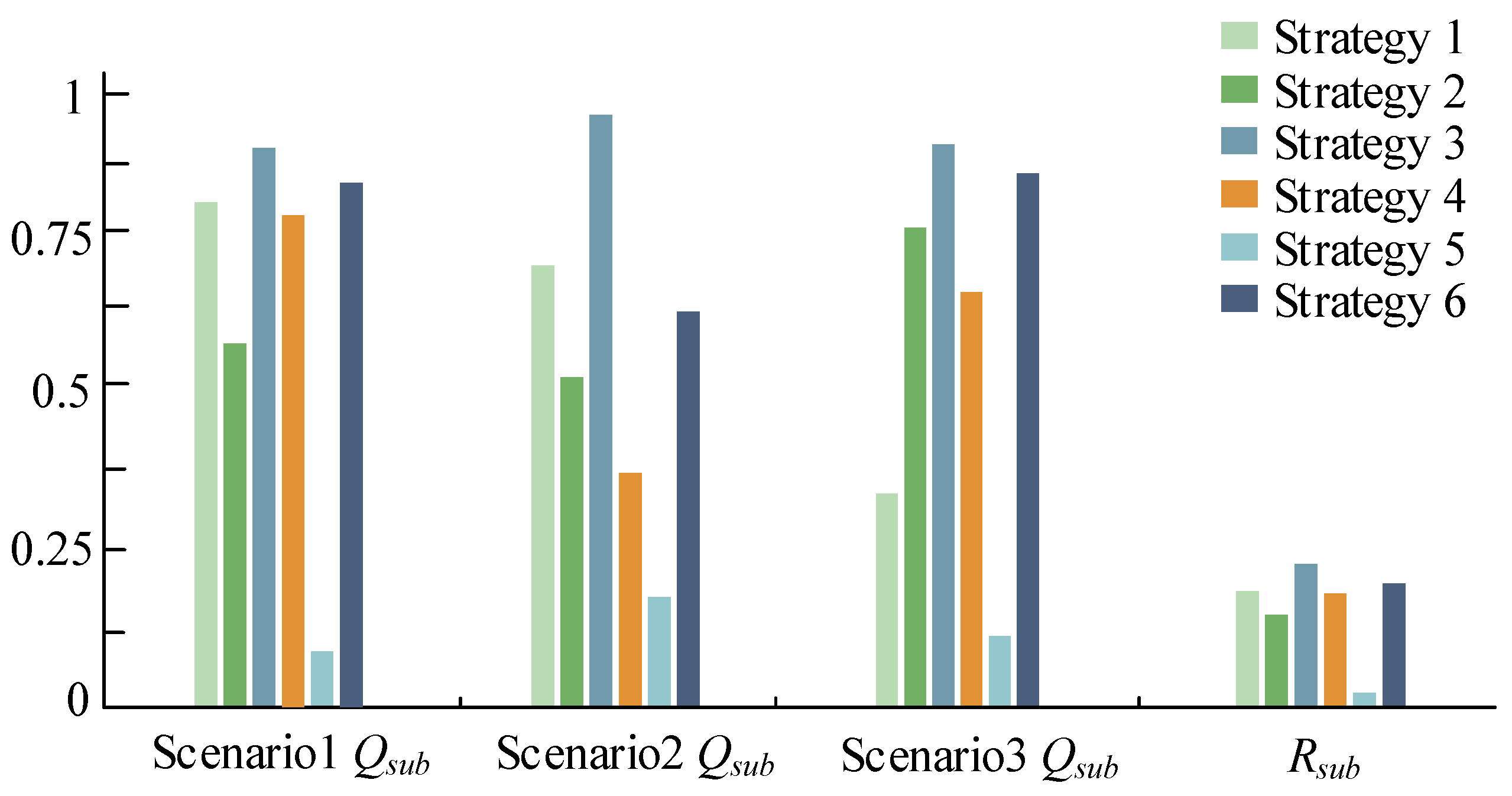
A comparative analysis was conducted using the three scenarios as case studies. Since THD is widely adopted as a core evaluation indicator, a weight of 0.7 was assigned to the THD reduction rate η%, 0.1 to the I_dc, 0.1 to the σ², and 0.1 to the α. To ensure a fair comparison, the same max-min normalization method as used in this paper was adopted for data preprocessing, and the preprocessed data were consistent with those listed in

Table A1. Weighted evaluation indicators in Scenario 1.

	α	η%	σ2	Idc
Strategy 1	0.0149	0.1522	0.1657	0.1165
Strategy 2	0.1044	0.1058	0.0843	0.098
Strategy 3	0.0888	0.1638	0.1823	0.1751
Strategy 4	0	0.1401	0.173	0.1563
Strategy 5	0.4788	0	0	0
Strategy 6	0.2566	0.1391	0.1799	0.1676

,

Table A2. Weighted evaluation indicators in Scenario 2.

	α	η%	σ2	Idc
Strategy 1	0.373	0.1399	0.147	0.1297
Strategy 2	0.1104	0.1148	0.1024	0.1292
Strategy 3	0.2426	0.2161	0.1925	0.2061
Strategy 4	0	0.0818	0.1312	0.0867
Strategy 5	0.0675	0	0	0
Strategy 6	0.0717	0.1226	0.1933	0.2176

and

Table A3. Weighted evaluation indicators in Scenario 3.

	α	η%	σ2	Idc
Strategy 1	0	0.1459	0.1548	0.0536
Strategy 2	0.1437	0.1545	0.1781	0.2517
Strategy 3	0.0899	0.2014	0.2005	0.2884
Strategy 4	0.2988	0.1365	0.1361	0
Strategy 5	0.1094	0	0	0.221
Strategy 6	0.1263	0.1766	0.1865	0.2993

. For the robustness evaluation, based on subjective experience, the performance indicator of Scenario 1 was also regarded as the most important indicator. A weight of 0.8 was assigned to the Q_sub1, 0.1 to the Q_sub2, and 0.1 to the Q_sub3. The evaluation results are presented in

Table 7. Performance and robustness evaluation results of all strategies under the three scenarios.

	Scenario 1 Qsub	Scenario 2 Qsub	Scenario 3 Qsub	Rsub
Strategy 1	0.811	0.6887	0.602	0.1979
Strategy 2	0.5761	0.5136	0.758	0.1496
Strategy 3	0.9186	0.9593	0.9265	0.2349
Strategy 4	0.7829	0.3726	0.6425	0.1852
Strategy 5	0.1	0.0181	0.1104	0.0236
Strategy 6	0.8423	0.6162	0.8491	0.2088

and Figure 19.

As shown in Table 7 and Figure 19, Strategy 3 outperforms Strategy 6 across all three scenarios, and the overall performance ranking trend of the strategies is fully consistent with the variation trend of the THD reduction rate indicator η%. Furthermore, as the Q_sub performance index in Scenario 1 is assigned the highest weight in the robustness evaluation, the robustness results are fully consistent with the variation trend of Q_sub in Scenario 1. These performance and robustness results exhibit significant discrepancies with the previous results obtained via the conventional entropy weight method, which demonstrates that the evaluation method proposed in this paper offers stronger applicability, higher evaluation accuracy, and a more objective analytical perspective.

6. Conclusions

Based on the above analysis, this paper developed a comprehensive performance and robustness evaluation method for resonance suppression strategies in PV grid-connected systems using the entropy weight method. By constructing resonance scenarios and evaluation indicators, multiple suppression strategies were evaluated under different scenarios using the entropy weight method. Meanwhile, the effectiveness of the indicators was verified under different operating conditions within a single scenario. The main conclusions are as follows:

(1) The constructed characteristic indicators, including the attenuation factor α, the variance σ² of the steady-state main resonant current peak, the total resonant current THD reduction rate η%, and the comprehensive performance indicator Q_s, are applicable to different resonance scenarios and various suppression strategies, which verifies the correctness of the proposed method for constructing performance characteristic indicators.

(2) A comprehensive performance and robustness evaluation method for resonance suppression strategies in PV grid-connected systems was proposed based on the entropy weight method. In terms of suppression performance, this method provides a basis for the selection of suppression strategies and feedback functions under the same resonance scenario. In terms of adaptability, it offers guidance for choosing appropriate suppression strategies under different application scenarios. The results demonstrate the accuracy of the evaluation method proposed in this paper.

(3) By comparing the evaluation results of the proposed method with those of the subjective weighting method, it is verified that the proposed method has more significant advantages and stronger objectivity in multi-scenario evaluation. The proposed method provides a theoretical basis for the performance evaluation of resonance suppression strategies designed with parameter adaptive algorithms, and helps to optimize the comprehensive performance and robustness of such strategies.

References

1. Angizeh, F.; Bae, J.; Chen, J.; Klebnikov, A. Impact Assessment Framework for Grid Integration of Energy Storage Systems and Renewable Energy Sources Toward Clean Energy Transition. IEEE Access 2023, 11, 134995–135005. [Google Scholar] [CrossRef] [Scilit]
2. Kang, Z.; Duan, R.; Zheng, Z.; Xiao, X.; Shen, C.; Hu, C.; Tang, S.; Qin, W. Grid Aided Combined Heat and Power Generation System for Rural Village in North China Plain Using Improved Pso Algorithm. J. Clean. Prod. 2024, 435, 140461. [Google Scholar] [CrossRef] [Scilit]
3. Enslin, J.H.R.; Heskes, P.J.M. Harmonic interaction between a large number of distributed power inverters and the distribution network. IEEE Trans. Power Electron. 2004, 19, 1586–1593. [Google Scholar] [CrossRef] [Scilit]
4. Chen, C.; Du, W.; Wang, H.; Littler, T. Sub-synchronous oscillations in power systems caused by grid-connected wind farms—A survey of mechanism studies. CSEE J. Power Energy Syst. 2018, 4, 495–503. [Google Scholar] [CrossRef] [Scilit]
5. Liu, D.S.; Xiong, S.; Song, Z.; Qiu, H. Review of Harmonic Suppression Technology Based on Photovoltaic Grid-connected Inverter. J. Electr. Eng. 2025, 20, 223–238. [Google Scholar]
6. Wan, C.; Li, K.; Xu, L.; Xiong, C.; Wang, L.; Tang, H. Investigation of an Output Voltage Harmonic Suppression Strategy of a Power Quality Control Device for the High-End Manufacturing Industry. Micromachines 2022, 13, 1646. [Google Scholar] [CrossRef] [Scilit] [PubMed]
7. Barva, A.V.; Joshi, S. Comparative Analysis of Passive, Active, and Hybrid Active Filters for Power Quality Improvement in Grid-Connected Photovoltaic System. In 2023 7th International Conference on Computer Applications in Electrical Engineering-Recent Advances (CERA); IEEE: Piscataway, NJ, USA, 2023; pp. 1–6. [Google Scholar]
8. Liu, Z.; Yuan, Y.; Liu, C.; Sun, C.; Bin, Z. Design and Optimization of a High-Frequency Oscillation Suppression Strategy for the Grid-Connected Inverter of a Permanent Magnet Direct Drive Wind Turbine. Energies 2025, 18, 1679. [Google Scholar] [CrossRef] [Scilit]
9. Sun, H.; Yao, W.; Shi, H.; Qin, L.; Deng, Y.; Liu, K. High-Frequency Oscillation Suppression Strategy for VSG MMC-HVDC Integrated Offshore Wind Farms Considering Frequency Coupling. Sensors 2026, 26, 1484. [Google Scholar] [CrossRef] [Scilit] [PubMed]
10. Li, Y.; Zhao, L.; Zhou, B.; Chen, Y.; Chen, Y.; Shentu, Z.; Yuan, H.; Du, W.; Zhang, X.; Li, C. Robustness Evaluation of Oscillation Suppression Strategies for Doubly-Fed Wind Power Grid-Connected Systems. In Proceedings of the 2025 IEEE 8th International Electrical and Energy Conference (CIEEC), Changsha, China, 16–18 May 2025; pp. 285–290. [Google Scholar]
11. Chen, Z.P.; Xie, N. Vulnerability Evaluation and Robustness Improvement Strategy of Complex Power Network Based on Fractal Mechanism. Power Syst. Technol. 2022, 45, 657–664. [Google Scholar]
12. Aggarwal, V.; Gupta, S. Optimizing Solar Panel Selection: A Comparative Analysis using AHP, Entropy, and Equal Weights in TOPSIS Methodologie. In 2023 Second IEEE International Conference on Measurement, Instrumentation, Control and Automation (ICMICA); IEEE: Piscataway, NJ, USA, 2021; pp. 1–5. [Google Scholar]
13. Hu, F.N.; Yang, W.D.; Chen, J. Robustness Assessment of Cyber-physical Power Systems Based on Critical Nodes. Complex Syst. Complex. Sci. 2024, 22, 43–49. [Google Scholar]
14. Zhou, D.Y.; Hu, F.N.; Chen, J. Robustness analysis of power system based on a complex network. Power Syst. Prot. Control 2023, 1, 72–80. [Google Scholar]
15. Li, G.; Zhou, M. Comprehensive evaluation model of wind power accommodation ability based on macroscopic and microscopic indicators. Prot. Control Mod. Power Syst. 2019, 4, 1–12. [Google Scholar] [CrossRef] [Scilit]
16. Zhang, L.; Zhu, S.; Si, R.; Yu, L.; Shao, H.; Yuan, Z. An Improved Fast Fitting Algorithm for PV Curves of Power Systems Based on the Least Squares Method. Lamps Light. 2024, 5, 102–104. [Google Scholar]
17. Ni, H.; Zhong, L.; Song, H.X. Moving least square curve and surface fitting with interpolation conditions. In 2010 International Conference on Computer Application and System Modeling; IEEE Computer Society: Washington, DC, USA, 2010; Volume 13, pp. 300–304. [Google Scholar]
18. Duan, J.; Chen, T.; Shang, D.; Cui, S.; He, Y. Current Attenuation Factor Based Line Protection Scheme for Distribution Network of DFIG Wind Power Integration System. Proc. CSEE 2020, 40, 1915–1924. [Google Scholar]
19. Qin, T.; Liu, M.; Ji, S.; Cai, D. Parameter Weight Analysis of Synchronous Induction Electromagnetic Coil Launch System Based on the Entropy Weight Method. IEEE Trans. Plasma Sci. 2023, 52, 1865–1873. [Google Scholar] [CrossRef] [Scilit]
20. Gao, J.Q.; Zhang, H.; Wei, R.G. Capacity Optimization of Wind-Solar-Diesel-Storage Complementary Power Generation System Based on Entropy Weight-TOPSIS Method. J. Chin. Soc. Power Eng. 2025, 2, 300–306. [Google Scholar]
21. Zhang, Q.; Wu, H.F.; Mei, X.J. A Sparse Sensor Placement Strategy Based on Information Entropy and Data Reconstruction for Ocean Monitoring. IEEE Internet Things J. 2023, 10, 19681–19694. [Google Scholar] [CrossRef] [Scilit]
22. Zhang, S.; Liu, K.; Zhang, S.; Xu, L. Study on Aerodynamic Performance and Lightweight Multiobjective Optimization Design of Wheel With Entropy Weighted Grey Relational Analysis Methods. IEEE Access 2022, 10, 93421–93438. [Google Scholar] [CrossRef] [Scilit]
Figure 1. Topology and control structure diagram of LCL-type PV grid-connected system.
Energies 19 01886 g001
Figure 2. PV grid-connected system with SVG.
Energies 19 01886 g002
Figure 4. Amplitude–frequency responses of two feedback functions.
Energies 19 01886 g004
Figure 5. Currents and fitting curves under different virtual impedances.
Energies 19 01886 g005
Figure 6. THD curves under different virtual impedances.
Energies 19 01886 g006
Figure 7. Diagrams of various performance indicators.
Energies 19 01886 g007
Figure 8. The peak values of resonant current under four types of virtual impedances.
Energies 19 01886 g008
Figure 9. Main resonant current and fitting curves of different strategies.
Energies 19 01886 g009
Figure 10. THD curves under different strategies.
Energies 19 01886 g010
Figure 11. The original performance indicators under Scenario 1.
Energies 19 01886 g011
Figure 12. THD curves under different strategies.
Energies 19 01886 g012
Figure 13. Main resonant current and fitting curves of different strategies.
Energies 19 01886 g013
Figure 14. The original performance indicators under Scenario 2.
Energies 19 01886 g014
Figure 15. Main resonant current and fitting curves of different strategies.
Energies 19 01886 g015
Figure 16. THD curves under different strategies.
Energies 19 01886 g016
Figure 17. The original performance indicators under Scenario 3.
Energies 19 01886 g017
Figure 18. The comprehensive performance and robustness of multiple strategies under different scenarios.
Energies 19 01886 g018
Figure 19. The comprehensive performance and robustness of multiple strategies under different scenarios.
Energies 19 01886 g019