Energy Management for a Fuel Cell Hybrid-Powered Unmanned Aerial Vehicle Based on Optimal Path Planning

Abstract

Unmanned Aerial Vehicles (UAVs) present a promising solution for urban logistics, where an effective energy management strategy guided by optimal path planning is crucial for reducing operational costs and extending system lifespan. This study begins by analyzing the wind field distribution in a specific urban area of Chengdu using Computational Fluid Dynamics, and establishes a data-driven power prediction model to evaluate UAV energy consumption. A hybrid wind-field-aware A* with Ant Colony Optimization algorithm is subsequently proposed to compute the optimal flight path that balances energy consumption and distance, generating corresponding power demand profiles for the ensuing energy management strategy. Finally, a Deep Q-Learning (DQN)-based energy management strategy is implemented to regulate power distribution between the fuel cell and the battery, aiming to minimize hydrogen consumption and stabilize the power output of the primary source. Experimental results demonstrate that the proposed path planning method can effectively reduce energy consumption across different scenarios while causing only a marginal increase in travel distance. In addition, the DQN-based strategy significantly suppresses fuel cell power fluctuations at the cost of only a slight increase in hydrogen consumption, thereby demonstrating the effectiveness of the path-planning-informed energy management strategy.

1. Introduction

Unmanned Aerial Vehicles (UAVs) are a promising solution for urban “last-mile” logistics, owing to their high maneuverability and independence from ground traffic [1]. However, their power systems must meet conflicting mission requirements: high power density for dynamic maneuvers such as takeoff and landing, and high energy density for sustained cruising. While lithium-ion batteries offer high power density, their energy density is limited; conversely, fuel cells provide high energy density but suffer from slow power response [2]. As a result, a hybrid power system that integrates both energy sources represents the most viable architecture to satisfy the full mission profile [3].

The performance of a UAV hybrid power system hinges critically on its Energy Management Strategy (EMS), which governs the intelligent power allocation between energy sources to minimize operational costs and extend system lifespan. Existing EMS approaches for UAVs can be broadly categorized into rule-based [4,5,6,7,8], optimization-based [9,10,11,12,13], and learning-based methods [14,15,16]. Due to their dependence on predetermined rules for power distribution, rule-based EMS strategies often fail to adapt effectively to complex flight conditions. Optimization-based methods aim to find globally optimal solutions to allocate the power, but they generally suffer from high computational burdens. Learning-based strategies, especially deep reinforcement learning (RL), have been introduced into energy management for UAV hybrid power systems due to their ability to achieve a superior trade-off between control optimality and computational efficiency, effectively handling system nonlinearity, environmental uncertainty, and high-dimensional state spaces. A health-aware strategy based on a Safe Deep Reinforcement Learning framework was proposed to minimize component degradation costs, including fuel cell voltage drop and battery capacity fade [14]. A Clipped Proximal Policy Optimization agent was used to optimize power distribution while ensuring engine operational safety and reducing speed fluctuations [15]. An RL-based framework was developed to minimize overall energy consumption by dynamically optimizing the vehicle’s power control system based on mission objectives and environmental conditions [16].

Current EMS research is largely confined to standardized cyclic flight patterns and consequently cannot be directly extended to mission-specific trajectories. Extensive research has been conducted on path planning to ensure the operational efficiency and safety of UAVs in complex logistics scenarios [17,18]. However, there has been limited research on integrating path planning with EMS to enhance overall system performance. A discrete graph was constructed by sampling the boundaries of quiet zones, and a sampling-based algorithm was utilized to simultaneously optimize the flight path and energy management by scheduling the mode switching between gasoline and electric power [19]. An adaptive Sequential Convex Programming method was proposed to solve the coupled model of trajectory optimization and energy management, which jointly optimizes the flight path to maximize solar energy capture while regulating the power allocation among the photovoltaic system, fuel cell, and battery [20]. A coordinated optimization method was developed to integrate flight trajectory and energy management, utilizing Fuzzy Neural Network Sequential Convex Programming to maximize solar energy utilization and a Convex Quadratic Programming Model Predictive Control strategy for real-time power allocation [21].

However, these studies overlook the impact of the wind field on path planning, which can lead to suboptimal power curves. Moreover, current integrated strategies rarely consider the impact of trajectory-induced power fluctuations on the degradation of the hybrid power system, leading to reduced component lifespan and operational reliability. Given the aforementioned issues, this research makes three key contributions to the field of urban drone logistics:

Novel Holistic Optimization Framework: A holistic framework that integrates wind-inclusive path planning with health conscious, multi-objective energy management is developed.

Power-Cognizant Trajectory Planning: By incorporating a wind-influence factor, hybrid A*-Ant Colony Optimization (HA*-ACO) algorithm is proposed to generate the optimized power demand profiles that serve as critical inputs for subsequent energy management.

Component-Aware Energy Strategy: The resulting energy management system implicitly incorporates component degradation factors, thereby enhancing both economic viability and operational reliability.

The remainder of this paper is organized as follows. Section 2 analyzes the problem and outlines the operational workflow of the logistics mission. Section 3 details the wind-affected flight models and introduces the proposed hybrid path planning method. Section 4 establishes the hybrid power system model and describes the DQN-based energy management strategy. Section 5 presents the experimental validation and results, and the paper is concluded in Section 6.

2. Problem Analysis

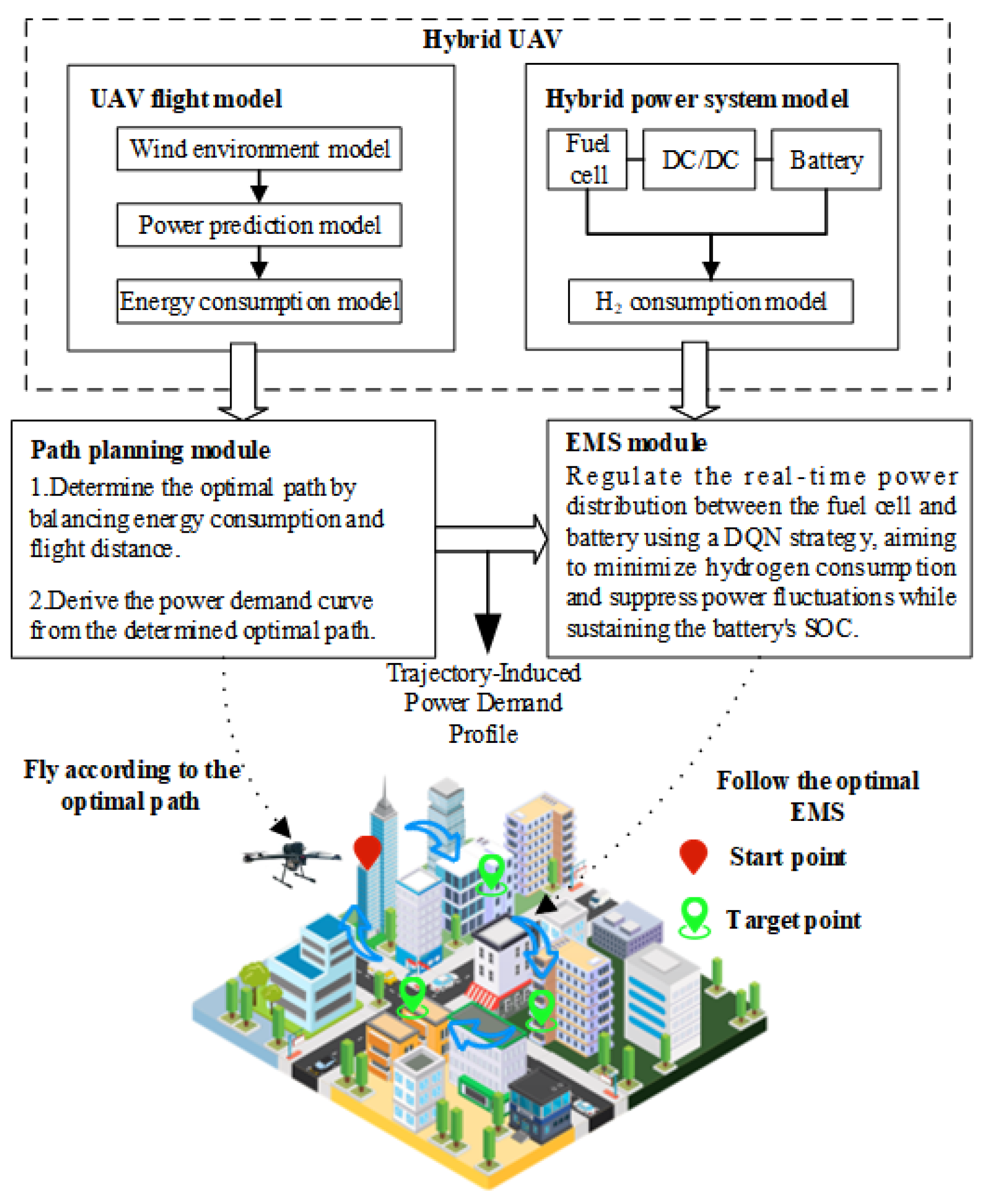
The workflow for the fuel cell hybrid UAV performing urban logistics delivery missions, as depicted in Figure 1, can be broadly divided into two main stages:

Path Planning Stage: A comprehensive UAV flight model is established, incorporating wind environment simulation, power prediction, and energy consumption models to derive the power requirements of the aircraft. Given start and destination points, the optimal flight path is computed by balancing energy consumption and travel distance. This stage also determines the visiting sequence and routes for all delivery points.

EMS Stage: A hybrid power system model is formulated, characterizing the fuel cell and battery to establish an H₂ consumption model. The energy management strategy first configures system capacities based on the UAV power curve. Subsequently, it utilizes the power demand curve to distribute power between the fuel cell and battery, with the objectives of minimizing hydrogen consumption, reducing fuel cell power fluctuations, and constraining battery state of charge (SOC) variations.

Although the workflow is divided into two sequential stages, it is important to emphasize that trajectory planning and energy management are not independent modules. The optimal flight trajectory directly determines the time-varying power demand profile through velocity evolution, altitude changes, and wind disturbances, and this trajectory-induced power demand profile serves as the primary input to the EMS stage.

3. System Modeling and Path Planning

3.1. Wind-Affected UAV Flight Model

Wind speed and wind direction are key factors influencing UAV power consumption. This study employs computational fluid dynamics (CFD) simulation to characterize the wind field distribution in the local urban environment, which includes the continuity equation, momentum conservation equations, and energy conservation equation [22]. The continuity equation describes the transport of fluid mass, while the momentum equations represent the fundamental physical processes of fluid motion, incorporating the effects of pressure gradients, viscous stresses, gravity, and external body forces. The energy equation characterizes the energy transfer processes within the fluid system. The CFD inputs include building geometry, inlet wind velocity, and atmospheric boundary layer conditions, and the wind speed and the wind direction are simulated through the following steps:

(1)

Based on the three-dimensional urban voxel grid model, a CFD computational domain of 1100 m × 700 m × 360 m is constructed. Following standard CFD modeling requirements, the domain boundaries are positioned at least 5H (300 m) away from the building cluster, where H represents the maximum building height (60 m). This configuration ensures adequate flow development space and prevents boundary effects from influencing the flow field calculations within the target area.

(2)

The computational domain is spatially discretized using Finite Volume Method with hexahedral structured mesh. A two-level refinement strategy is implemented: minimum mesh size of 5 m × 5 m within the building group area, and 10 m × 10 m mesh size in surrounding areas.

(3)

Select the standard k-ε turbulence model and the boundary conditions are set as follows: velocity inlet with 5 m/s uniform wind on the windward side, pressure outlet on leeward side, no-slip walls for ground and building surfaces, and symmetry boundaries for top and lateral domain sides.

(4)

Governing equations are solved using Ansys Fluent 2023 R1 with SIMPLE algorithm for pressure-velocity coupling and second-order upwind scheme for spatial discretization. The convergence criteria requires a residual of less than 10⁻⁴.

3.2. Power Prediction

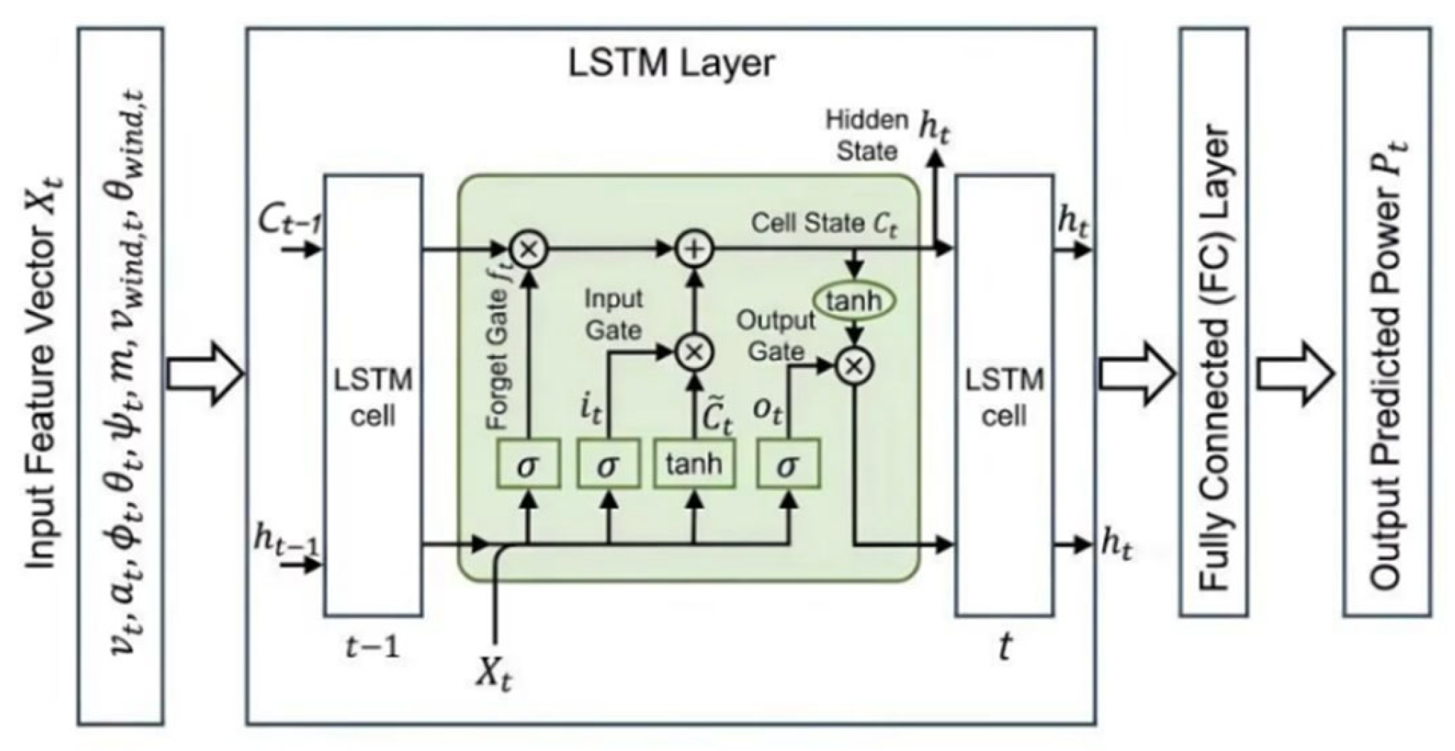
To accurately evaluate UAV energy consumption within complex urban wind fields, a data-driven power prediction model is established using a Long Short-Term Memory (LSTM) network. Unlike traditional Recurrent Neural Networks, the LSTM architecture effectively mitigates the vanishing gradient problem, enabling the capture of long-term temporal dependencies inherent in nonlinear flight power profiles. The schematic of the proposed framework is illustrated in Figure 2.

UAV power consumption results from the coupling of kinematic states and external environmental disturbances. To characterize this, the input feature vector $X_t$ at time step $t$ is constructed by integrating flight dynamic parameters with CFD-simulated wind field data:

$$X_t=[v_t,a_t,{\varphi }_t,{\theta }_t,{\psi }_t,m,v_{wind,t},{\theta }_{wind,t}{]}^T$$

(1)

where $v_t$ and $a_t$ denote the magnitude of ground velocity and acceleration, respectively; ${\varphi }_t,{\theta }_t,{\psi }_t$ represent the roll, pitch, and yaw Euler angles; and $\mathrm{m}$ is the total aircraft mass. Critically, the environmental inputs $v_{wind,t}$ and ${\theta }_{wind,t}$ (wind speed and direction) are derived directly from the CFD simulation, allowing the model to account for aerodynamic power variations caused by local wind field non-uniformity.

The prediction framework comprises three functional modules: the input layer, the LSTM feature extraction layer, and the fully connected output layer. The sequence of input vectors $X_t$ is fed into the LSTM layer. Leveraging its internal gating mechanisms (input, forget, and output gates), the LSTM unit regulates the information flow, selectively retaining historical flight states in the cell state $C_t$. This process generates a hidden state $h_t$ that encodes the complex, time-varying correlations between flight maneuvers, wind disturbances, and power demand.

The LSTM model establishes a nonlinear mapping from the input feature vector $X_t$ to the predicted instantaneous power $P_t$, which can be expressed as:

$$P_t=f_{LSTM}\left(X_t\right)$$

(2)

All weight matrices and bias vectors involved in the LSTM and fully connected layers are trainable parameters, which are automatically optimized during the network training process. The model is trained using the Adam optimization algorithm with a learning rate of 0.001 and a batch size of 128, optimizing the network parameters to minimize the Mean Squared Error between the predicted and actual measured power profiles.

The LSTM model is developed and evaluated using a documented power consumption dataset for a DJI Matrice 100 UAV [23]. The first 100 flight records from this dataset are partitioned into training and validation sets with a ratio of 8:2, while two distinct flight records, separate from these, are reserved as an independent test set to evaluate the model’s ability to generalize. The input to the LSTM model at each time step comprises the UAV’s previous flight state variables—including velocity (0.0–18.5 m/s), acceleration (−3.8 to 4.2 m/s²), yaw angle (−82.7° to 65.9°), pitch angle (−21.1° to 26.5°), and roll angle (−10.5° to 14.4°)—along with environmental conditions such as wind speed (0.0–9.6 m/s) and wind direction (0.0–359.9°).

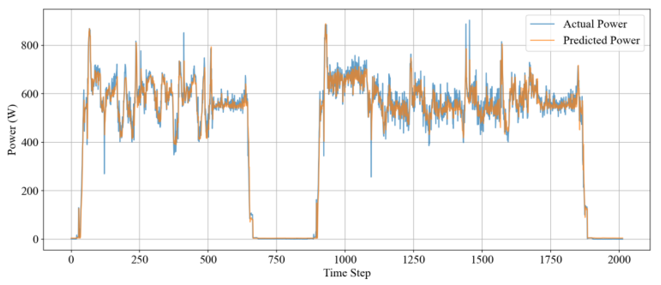
The prediction performance on the independent test set is presented in Figure 3. This figure illustrates the comparison between the actual recorded power consumption and the model’s predicted power over a series of time steps. Power values near 0 W correspond to periods when the UAV is on the ground either pre-takeoff or post-landing. During flight operations, the power consumption generally fluctuates between approximately 400 W and 800 W. The lower end of this range typically represents hovering or stable, low-speed flight, while the higher values indicate more demanding maneuvers such as rapid acceleration, climbing, or compensating for strong winds. The figure visually confirms that the model accurately tracks these actual power variations, maintaining high fidelity even during periods of significant and rapid fluctuation. This strong predictive performance is quantitatively validated by an RMSE of 42.99 W and an R² of 0.95 on the test set, confirming the model’s high accuracy and generalization capability. The LSTM power prediction model is trained and evaluated using flight data covering wind speeds from 0.0 to 9.6 m/s and wind directions from 0.0° to 359.9°. Higher wind speeds increase aerodynamic drag and require more power to maintain speed or altitude, while strong headwinds lead to higher power consumption during flight, whereas tailwinds can reduce power needs.

3.3. UAV Energy Consumption Model

In the context of logistics delivery missions within urban environments, the total energy consumption $E(n_u,n_v)$ between any two consecutive path points $n_u$ and $n_v$ is calculated by integrating power consumption over different flight phases, which is calculated as follows:

$$E(u,v)=E_{acc}+E_{const}={\displaystyle \frac{(P_{UAV}^u+P_{UAV}^v)}{2}}\cdot \Delta t_{acc}+P_{UAV}^{uv}\cdot (\Delta t-\Delta t_{acc})$$

(3)

where $P_{UAV}^u$ and $P_{UAV}^v$ represent the UAV power at the start and end of the acceleration/deceleration phase, respectively; ${ P}_{UAV}^{uv}$ denotes the power maintained during the constant velocity phase; $\Delta t_{acc}$ is the duration of the acceleration/deceleration phase; and $\Delta t$ represents the total time elapsed between the two path nodes.

3.4. UAV Path Planning

As shown in Figure 1, given a set of delivery target nodes, the UAV is required to perform a logistics delivery mission that starts from a start node, visits all target nodes, and finally returns to the origin. In order to minimize the energy consumption and the flight distance during the delivery mission, the path planning task is decomposed into two hierarchical optimization problems: (1) local path optimization between pairs of target nodes; (2) global route optimization that determines the visiting sequence of target nodes.

For local path planning, the start node and the target node are given by the delivery task. Let $n_0$ denote the start node, and let $n_i$ and $n_j$ refer to the i-th and j-th target nodes, respectively, where i, j ∈ {0, 1, …, K}, $i\ne j$, and K is the total number of target nodes in the mission. For any two mission nodes $n_i$ and $n_j$, the objective is to determine a feasible path p from $n_i$ to $n_j$ that minimizes the accumulated edge cost. Therefore, the local path cost is defined as:

$$C_{ij}=\underset{p\in P(n_i,n_j)}{\min }{\displaystyle \sum _{(u,v)\in p}c}(u,v)$$

(4)

where $P(n_i,n_j)$ represents the set of all feasible paths from node $n_i$ to node $n_j$, and p is a feasible path in this set; u and v denote two adjacent nodes along path p; c$(u,v)$ is the cost of traversing the edge between two adjacent nodes u and v, which is calculated as follows:

$$c(u,v)=\omega eD(u,v)+(1-\omega )E(u,v)$$

(5)

where $D(u,v)$ is the Euclidean distance between the two voxel nodes; $E(u,v)$ is the estimated energy consumption between the nodes, calculated using Equation (3); ω ∈ [0, 1] is the weighting coefficient that balances distance and energy objectives, e is a normalization factor used to scale distance and energy to comparable magnitudes.

In this study, this local path optimization problem is solved using a wind-aware A* algorithm. In a conventional A* algorithm, the Euclidean distance is typically used as the heuristic function. In this paper, a wind field factor $w_f$ is introduced to modify the heuristic function, enabling the search process to account for wind-induced energy variations. The evaluation function of the local path search is defined as follows:

$$f(x)={\displaystyle \sum _{(u,v)\in p}c}(u,v)+w_f(v_r,\theta )\sqrt{{(x_g-x_{n_j})}^2+{(y_g-y_{n_j})}^2+{(z_g-z_{n_j})}^2}$$

(6)

where p denotes the path from the mission node $n_i$ to the current node g; the coefficient $w_f(v_r,\theta )$ is a wind-field adjustment factor that modifies the heuristic distance according to the relative wind speed $v_r$ and the angle $\theta$ between the UAV’s flight direction and the wind direction; ($x_g$, $y_g$, $z_g$) denotes the coordinates of the current voxel node $g$, and ($x_{n_j}$, $y_{n_j}$, $z_{n_j}$) denotes the coordinates of the target node $n_j$.

After obtaining the locally optimal path using the A* algorithm, the remaining task is to determine the optimal visiting sequence of these nodes so as to minimize the total mission cost of the delivery tour:

$$\underset{\pi }{\min } F_{tour}={\displaystyle \sum _{i=0}^K{\displaystyle \sum _{j\ne i}^K{C}_{ij}}}{x}_{ij}$$

(7)

where $\mathsf{\pi }$ is the visiting sequence of target nodes which is defined as $\pi =\{n_0,n_1,n_2,\dots ,n_K,n_0\}$; $n_0$ is the starting nodes; $n_1,n_2,\dots ,n_K$ are the delivery target nodes; $x_{ij}$ is a binary decision variable defined as:

$$x_{ij}=\{\begin{array}{ll}1,& if the path segment from n_i to{n}_j is selected\\ 0,& otherwise\end{array}$$

(8)

The global route optimization problem then becomes a traveling salesman problem with energy-aware edge costs. To solve this problem, the ACO algorithm is employed to search for the optimal visiting sequence of the delivery nodes. The probability that ant k moves from node i to node j is defined as [24]:

$$p_{ij}^{\left(k\right)}={\displaystyle \frac{{[{\tau }_{ij}(t)]}^{\alpha }{[{\eta }_{ij}]}^{\beta }}{{\displaystyle \sum _{l\in K}[}{\tau }_{il}(t){]}^{\alpha }{[{\eta }_{il}]}^{\beta }}}$$

(9)

where ${\tau }_{ij}\left(t\right)$ denotes the pheromone concentration on edge $i\to j$; $\alpha$ and $\beta$ control the relative influence of pheromone and heuristic information; $K$ represents the set of selectable nodes; ${\eta }_{ij}$ is the heuristic value which is defined as the inverse of the path cost between two nodes:

$${\eta }_{ij}={\displaystyle \frac{1}{{\displaystyle \sum _{(u,v)\in p}c(u,v)}}}$$

(10)

Initially, pheromone values are distributed uniformly across all edges, allowing the ants to explore different candidate routes. As the iterations proceed, pheromone concentrations on high-quality paths are reinforced, enabling the algorithm to gradually converge toward an optimal visiting sequence. After each iteration, the pheromone values are updated according to the following rule:

$${\tau }_{ij}\left(t+1\right)=\left(1-\rho \right){\tau }_{ij}\left(t\right)+{\displaystyle \sum _{k=1}^n\Delta {\tau }_{ij}^k}$$

(11)

where $\rho$ is the pheromone evaporation coefficient; $\Delta {\tau }_{ij}^{\left(k\right)}={\displaystyle \frac{Q}{F_{tour}^{\left(k\right)}}}$ represents the pheromone increment deposited by ant k, and $F_{tour}^{\left(k\right)}$ denotes the tour cost obtained by ant k.

During the path planning process, the generated trajectories must satisfy the UAV’s kinematic and operational constraints to ensure flight feasibility and safety. In particular, the UAV velocity and acceleration are restricted within their allowable ranges. These constraints describe the physical flight limits of the UAV and guarantee that the planned paths can be executed by the vehicle during real flight operations. The corresponding constraints can be expressed as:

$$\begin{array}{c}{v}_{\min }\le v_t\le v_{\max }\\ a_{\min }\le a_t\le a_{\min }\end{array}$$

(12)

where ${ v}_{min}$ and ${ v}_{max }$ represent the UAV’s minimum and maximum velocity, respectively. Similarly, the UAV’s horizontal acceleration and vertical acceleration at ${ n}_{u }$ must not exceed their respective maximum values. The instantaneous velocity $v_t$ and acceleration $a_t$ are calculated as:

$$v_t=\sqrt{{\dot{x}}_t^2+{\dot{y}}_t^2+{\dot{z}}_t^2}$$

(13)

$$a_t={\displaystyle \frac{v_t-v_{t-1}}{\Delta t}}$$

(14)

where ${\dot{x}}_t, {\dot{y}}_t \mathrm{a}\mathrm{n}\mathrm{d} {\dot{z}}_t$ are the velocity components of UAV at time t which can be expressed as:

$${\dot{x}}_t={\displaystyle \frac{x_t-x_{t-1}}{\Delta t}}$$

(15)

$${\dot{y}}_t={\displaystyle \frac{y_t-y_{t-1}}{\Delta t}}$$

(16)

$${\dot{z}}_t={\displaystyle \frac{z_t-z_{t-1}}{\Delta t}}$$

(17)

where $x_t,y_t$ and ${ z}_t$ denote the spatial coordinates of the UAV at time t, which are taken from the optimal sequence of spatial nodes generated by the path planning stage.

Based on this discrete trajectory, the attitude angles ${\theta }_t, {\psi }_t \mathrm{a}\mathrm{n}\mathrm{d}{ \varphi }_{t }$ representing the pitch, yaw, and roll angles, respectively, can also be extracted from the trajectory geometry as follows [25]:

$${\theta }_t=\arctan ({\displaystyle \frac{{\dot{z}}_t}{\sqrt{x_t^2+y_t^2}}})$$

(18)

$${\psi }_t=\arctan 2({\dot{y}}_t,{\dot{x}}_t)$$

(19)

$${\varphi }_t=\arctan \left({\displaystyle \frac{v_t-{\stackrel{.}{\psi }}_t}{g}}\right)$$

(20)

where $g$ denotes the gravitational acceleration.

Furthermore the localized wind variables $v_{wind,t }$ and ${\theta }_{wind,t}$ are obtained by mapping each path point (x, y, z) to the CFD-based wind field model established in Section 2. These variables, including the UAV velocity $v_t$, acceleration $a_t$, attitude angles ${\theta }_t, {\psi }_t \mathrm{a}\mathrm{n}\mathrm{d}{ \varphi }_t$, local wind speed $v_{wind,t }$, and wind direction ${\theta }_{wind,t}$, are then fed into the pre-trained LSTM power prediction model to derive the corresponding UAV power demand profile $P_{req}\left(t\right)$.

4. DQN-Based EMS

4.1. Hybrid Power System Model

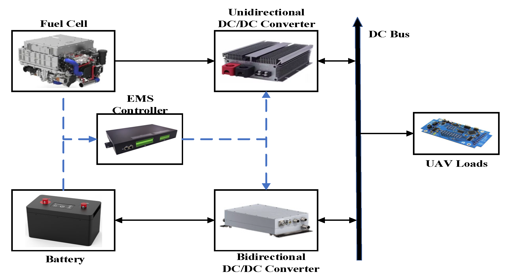
The topology of the hybrid power system is illustrated in Figure 4. Proton Exchange Membrane Fuel Cell (PEMFC) exhibits high efficiency and specific power characteristics, requires a short start-up time, and operates at low temperatures. Therefore, this study selects PEMFC as the main power source for the UAV power system. The lithium battery pack acts as the auxiliary/peak power source and energy buffering unit. The output voltage of the fuel cell stack is generally lower than the bus voltage, so a unidirectional DC/DC converter is used to boost the voltage before connecting to the bus. Meanwhile, the power battery not only supplies power to the system but also needs to absorb energy from the fuel cell for recharging when its SOC is low. Therefore, a bidirectional DC/DC converter is employed to enable two-way energy flow between the battery and the bus.

4.1.1. Fuel Cell

Complex nonlinear multi-input multi-output PEMFC models are difficult to be used for real-time EMS, Therefore, using cftool fitting in MATLAB R2022a, the power-efficiency relationship is established as follows:

$${\eta }_{fc}(P_{fc}(t))=-21.779474P_{fc}^3(t)+37.499668P_{fc}^2(t)-33.23206P_{fc}(t)+61.943587$$

(21)

where ${ P}_{fc}$ is output power of the fuel cell. Accordingly, the instantaneous hydrogen consumption rate is expressed as [26]:

$${\dot{m}}_{H_2, fc}(t)={\displaystyle \frac{P_{fc}(t)}{{\eta }_{fc}(P_{fc}(t))LH{V}_{H_2}}}$$

(22)

where $LH{V}_{H_2}$ is the lower heating value of hydrogen, representing the chemical energy released per unit mass of hydrogen during combustion (typically 120 MJ/kg). The total hydrogen consumption over the mission horizon is calculated as:

$$m_{H_2, fc}={\displaystyle \sum _{t=0}^{T-1}{\dot{m}}_{H_2, fc}}(t)\Delta t$$

(23)

where Δt is the sampling interval and T is the total number of time steps.

4.1.2. Lithium Battery

The SOC of the lithium battery reflects the ratio of its remaining capacity to its capacity and is modeled as in Equation (22):

$$SOC(t)=SOC(t-1)-A_n{\displaystyle \frac{P_{bat}(t)\Delta t}{E_{bat}}},\hspace{1em}{A}_n=\left\{\begin{array}{ll}{\eta }_{bat}\hfill & \mathrm{charging}\hfill \\ 1/{\eta }_{bat}\hfill & \mathrm{discharging}\hfill \end{array}\right.$$

(24)

where SOC(t) represents the battery state of charge at time step t; $P_{bat}$ is the lithium battery power; ${\eta }_{bat}$ is the lithium battery charge/discharge efficiency (98%); $E_{bat}$ is the lithium battery capacity.

4.1.3. DC/DC Converter

The DC/DC converters are mainly responsible for energy transfer and voltage regulation. However, this process inevitably involves some energy loss, which is expressed as follows:

$${\eta }_{DC/DC}={\displaystyle \frac{P_{\mathrm{in} }-P_{\mathrm{loss} }}{P_{\mathrm{in} }}}$$

(25)

where ${\eta }_{DC/DC}$ is the converter efficiency; $P_{in}$ is the input power, and $P_{loss}$ is the total power loss of the converter.

After considering converter losses, the bus-side powers of the fuel cell and the battery can be respectively expressed as:

$$P_{fc, bus}\left(t\right)={\eta }_{unDC}{P}_{fc}\left(t\right)$$

(26)

$$P_{bat, bus}(t)=\{\begin{array}{ll}{\eta }_{BidDC}{P}_{bat}\left(t\right),& P_{bat}\left(t\right)\ge 0\left(discharging\right)\\ {\displaystyle \frac{P_{bat}\left(t\right)}{{\eta }_{BidDC}}},& P_{bat}\left(t\right)<0\left(charging\right)\end{array}$$

(27)

where ${\eta }_{unDC}$ and ${\eta }_{BidDC}$ are the efficiencies of the unidirectional and bidirectional DC/DC converters, respectively.

4.2. EMS Optimization Objectives and Constraints

The objective of the EMS is to optimally allocate the power demand between the fuel cell system and the battery, so as to achieve high hydrogen economy while maintaining battery charge sustainability and reducing fuel cell load fluctuations. Therefore, the EMS problem is formulated as a multi-objective optimization problem as follows:

$$\underset{u(t)}{\min }J={\displaystyle \sum _{t=0}^{T-1}\left[\alpha {\dot{m}}_{H_2, fc}(u(t))\Delta t+\beta {(SOC(u(t))-SO{C}_{ref})}^2+\gamma \left|u(t)\right|\right]}$$

(28)

where u(t) is the control input; $\alpha$, $\beta$ and $\gamma$ are weighting coefficients, and $SO{C}_{ref}$ is the reference SOC. The first term represents the hydrogen consumption over the control interval. Reducing this term helps improve the fuel economy of the hybrid power system. The second term penalizes the deviation of the battery SOC from its reference value, so as to maintain the battery within a charge-sustaining operating range rather than allowing continuous depletion or excessive charging during the mission. The third term represents the variation in fuel cell output power, which can suppress abrupt load changes and reduce the dynamic operating stress of the fuel cell system, and can be calculated as follows:

$$u\left(t\right)=\Delta P_{fc}\left(t\right)$$

(29)

Thus, the fuel cell power is updated by:

$$P_{fc}\left(t\right)=P_{fc}(t-1)+u\left(t\right)$$

(30)

Based on Equations (22) and (30), the hydrogen consumption rate can be rewritten as:

$${\dot{m}}_{H_2, fc}(u(t))={\displaystyle \frac{P_{fc}(t-1)+u(t)}{{\eta }_{fc}(P_{fc}(t))LH{V}_{H_2}}}$$

(31)

The required power $P_{req}\left(t\right)$, generated during the path-planning stage, is supplied by the fuel cell and the lithium battery. Therefore, the EMS should satisfy the following power balance:

$$P_{req}\left(t\right)=P_{fc, bus}\left(t\right)+P_{bat, bus}\left(t\right)$$

(32)

Based on Equations (26), (30) and (32), the battery bus-side power can be calculated as follows:

$$P_{bat,bus}\left(t\right) =P_{req}\left(t\right)-{\eta }_{unDC}\left(P_{fc}(t-1)+u\left(t\right)\right)$$

(33)

By substituting Equation (33) into Equation (27), the battery power can be further expressed explicitly as a function of the control input u(t):

$$\begin{array}{r}{P}_{bat}(u(t))=\{\begin{array}{ll}{\displaystyle \frac{P_{req}\left(t\right)-{\eta }_{unDC}\left(P_{fc}(t-1)+u\left(t\right)\right)}{{\eta }_{BidDC}}},& P_{bat, bus}\left(t\right)\ge 0\\ {\eta }_{BidDC}\left(P_{req}\left(t\right)-{\eta }_{unDC}\left(P_{fc}(t-1)+u\left(t\right)\right)\right),& P_{bat, bus}\left(t\right)<0\end{array}\end{array}$$

(34)

Then, substituting $P_{bat}\left(t\right)$ into the battery SOC dynamics in Equation (24), the SOC update can be written explicitly as:

$$\begin{array}{r}SOC(t)=\{\begin{array}{l}SOC(t-1)-{\displaystyle \frac{\Delta t}{{\eta }_{bat}{\eta }_{BidDC}{E}_{bat}}}\left(P_{req}\left(t\right)-{\eta }_{unDC}\left(P_{fc}(t-1)+u\left(t\right)\right)\right),P_{bat, bus}\left(t\right)\ge 0\\ SOC(t-1)-{\displaystyle \frac{{\eta }_{bat}{\eta }_{BidDC}\Delta t}{E_{bat}}}\left(P_{req}\left(t\right)-{\eta }_{unDC}\left(P_{fc}(t-1)+u\left(t\right)\right)\right),P_{bat, bus}\left(t\right)<0\end{array}\end{array}$$

(35)

From the above derivations, each term in the optimization objective is related to u(t). In the optimization process of Equation (28), the following constraints must be satisfied:

(1) Fuel cell power increment constraint

$$0\le P_{fc}(u(t))\le P_{fc}^{\max }$$

(36)

where $P_{fc}^{\mathrm{m}\mathrm{a}\mathrm{x}}$ is the maximum output power of the fuel cell system. This constraint ensures that the fuel cell always operates within its allowable power range.

(2) Battery power constraint

$$P_{bat}^{\min }\le P_{bat}(u(t))\le P_{bat}^{\max }$$

(37)

where $P_{bat}^{\mathrm{m}\mathrm{i}\mathrm{n}}<0$ and $P_{bat}^{\mathrm{m}\mathrm{a}\mathrm{x}}>0$ denote the charging and discharging power limits of the battery, respectively. This constraint prevents the battery from exceeding its allowable charging and discharging power limits.

(3) Battery SOC constraint

$$SO{C}^{\min }\le SOC(u(t))\le SO{C}^{\max }$$

(38)

where $SO{C}^{\mathrm{m}\mathrm{i}\mathrm{n}}$ and $SO{C}^{\mathrm{m}\mathrm{a}\mathrm{x}}$ are its lower and upper bounds, respectively. This constraint keeps the battery SOC within a safe operating range to avoid over-charge and over-discharge.

4.3. Design of DQN-Based EMS

To address the energy management optimization problem within a continuous state space, this study adopts DQN algorithm. DQN integrates the strengths of Q-Learning with deep neural networks by approximating the action-value function Q(s, a) via a neural network, thereby enabling the effective handling of high-dimensional state inputs and the learning of optimal control strategies.

Key variables reflecting the UAV flight status and the health of the hybrid power system are selected to construct the state vector. At time step t, the state $s_t$ is defined as:

$$s_t=\left\{SOC(t),P_{fc}(t),P_{req}(t),v(t)\right\}$$

(39)

To ensure smooth control and protect the fuel cell from rapid power fluctuations, the action $a_t$ is defined as the change in the fuel cell’s output power $\Delta P_{fc}$. The continuous range of this change is uniformly discretized into 9 distinct actions spanning the interval [−0.2, 0.2] kW, as presented in Equation (40):

$$a_t=\left\{-0.2,-0.15,-0.1,-0.05,0,0.05,0.1,0.15,0.2\right\}(\mathrm{kW})$$

(40)

The agent selects an action $a_t$ at each time step, and the fuel cell power for the subsequent moment is updated as:

$$P_{fc}\left(t\right)=P_{fc}(t-1)+a_t$$

(41)

The reward function is critical as it encodes the multi-objective optimization problem into the RL framework. It is formulated as the negative of a weighted cost function that reflects the system’s lifecycle operating cost, which is given as follows:

$$r_t=-(\left[\alpha { \dot{\mathrm{m}} }_{H_2, fc}(t)\Delta t+\beta {(SOC(\mathrm{t})-SO{C}_{ref})}^2+\gamma \left|\Delta P_{fc}(t)\right|\right])$$

(42)

The objective of the DQN algorithm is to learn the optimal action–value function, which represents the expected cumulative discounted reward obtained by taking action a in state s and subsequently following the optimal policy:

$$Q^{*}(s,a)=\mathbb{E}[r_t+\gamma \underset{\mathit{a}\prime }{\mathit{max}}Q(s_{t+1},a\prime )|s_t=s,a_t=a]$$

(43)

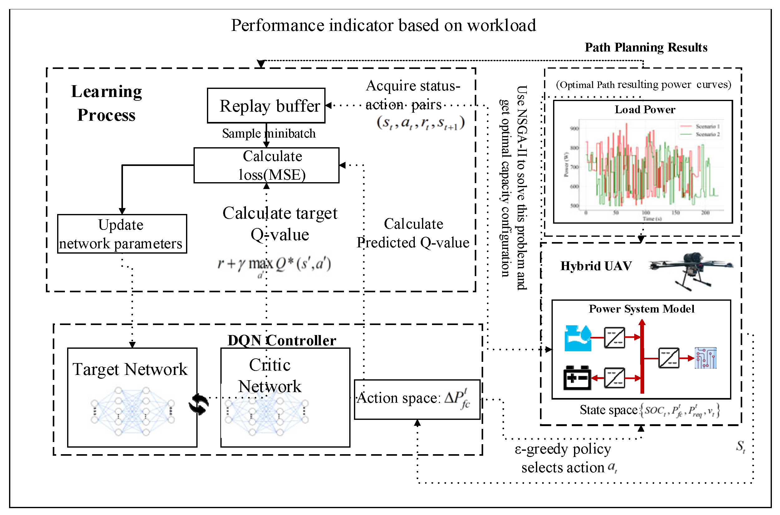
In this study, the DQN-based EMS follows the standard off-policy learning procedure illustrated in Figure 5. At each time step, the agent first observes the current system state $s_t$. Based on an ε-greedy policy, an action $a_t$, representing the increment of fuel cell power $\Delta P_{fc}\left(t\right)$, is selected from the discrete action space. The selected action is then applied to the hybrid power system model, resulting in the next state $s_{t+1}$ and an immediate reward ${\mathrm{r}}_{\mathrm{t}}$. The transition tuple $(s_t,a_t,r_t,s_{t+1})$ is stored in the replay buffer.

During training, minibatches of transitions are randomly sampled from this buffer to reduce temporal correlation among data samples. For each sampled transition, the target Q-value $y_t$ is computed using the target network:

$$y_t=r_t+\gamma \underset{\mathit{a}\prime }{\mathit{max}}\widehat{Q}(s\prime ,a\prime ;\theta \prime )$$

(44)

where $\mathsf{\gamma }$ ∈ (0, 1) is the discount factor that determines the importance of future rewards; $\widehat{\mathrm{Q}}$ is the Q-value of the target network; $\mathrm{s}\prime$ represents the next state; $a\prime$ denotes a candidate action in the action space; $\mathsf{\theta }\prime$ denotes the parameters of the target network. The mean squared error between the predicted Q-value and the target Q-value is defined as follows:

$$L(\theta )={\mathbb{E}}_{(s,a,r,s\prime )\sim D}[{\left(y_t-Q(s,a;\theta )\right)}^2]$$

(45)

where $L\left(\theta \right)$ is the loss function; $\theta$ denotes the parameters of the main Q-network and it is updated by minimizing $L\left(\theta \right)$; $\mathbb{E}$ represents the expectation; $(s,a,r,s\prime )\sim D$ means that the transition tuple is randomly sampled from this buffer; $Q(s,a;\theta )$ is the predicted Q-value produced by the main Q-network.

5. Experiments and Analysis of Results

5.1. Path Planning Results

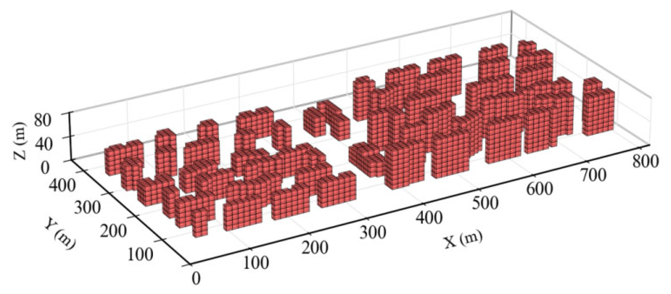
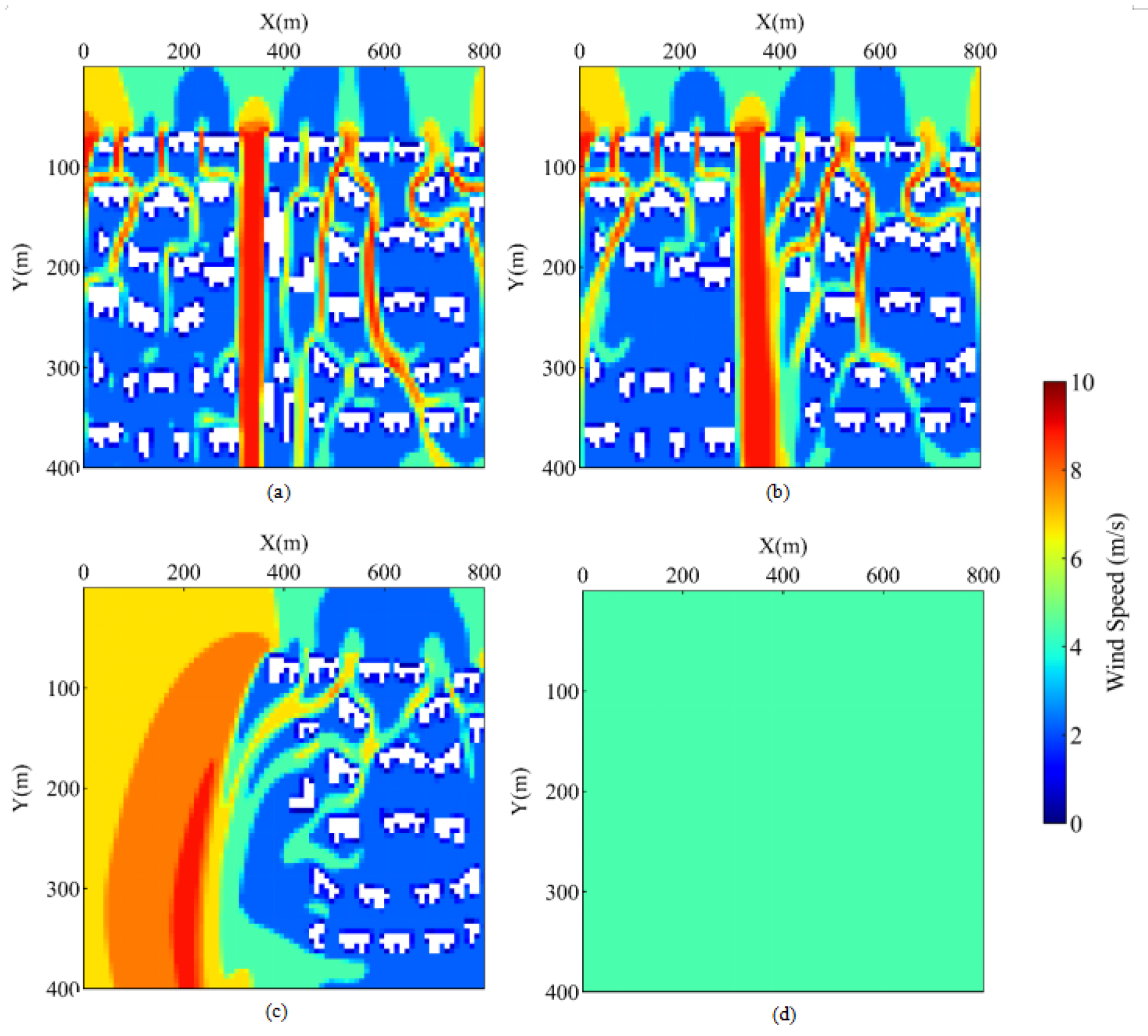
The proposed method is evaluated in a residential area of Chengdu with dimensions of 800 × 400 × 80 m, which is discretized into a three-dimensional voxel grid. A detailed 3D voxel-based geometric model is constructed using Ansys SpaceClaim, as illustrated in Figure 6. CFD simulations are conducted under representative north wind conditions to characterize the urban wind environment. The simulation results indicate distinct wind field distributions across four altitude intervals: 0–26 m, 27–36 m, 37–60 m, and 61–80 m. Figure 7 illustrates the horizontal wind field distributions corresponding to these height ranges and under the north-wind condition, the steady-state simulation required approximately 4.8 h to converge to a residual threshold of 10⁻⁴. The results reveal that lower altitudes show high non-uniformity with channeling effects and wake zones, while higher altitudes approach uniform free-stream conditions as building influence diminishes.

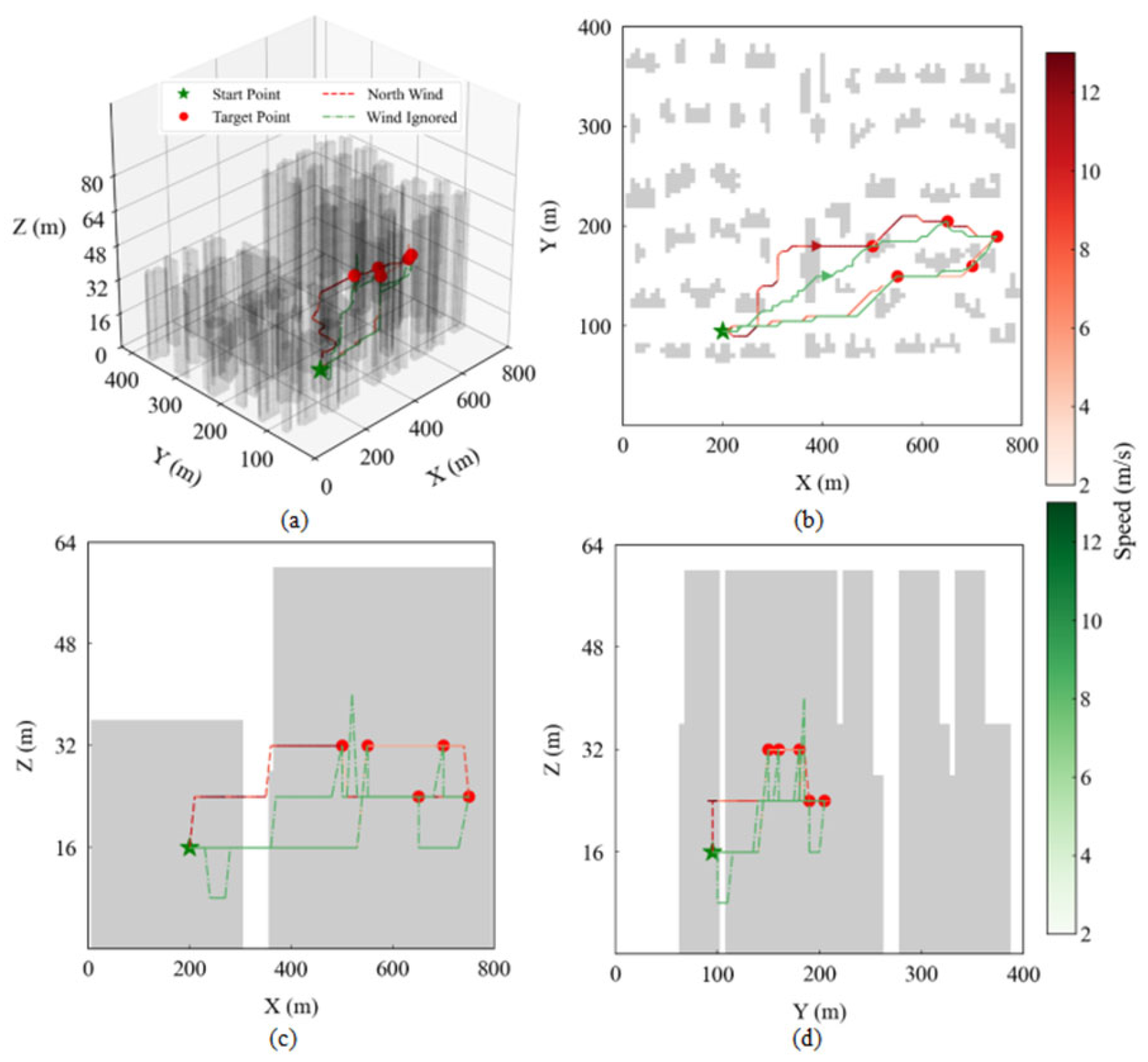
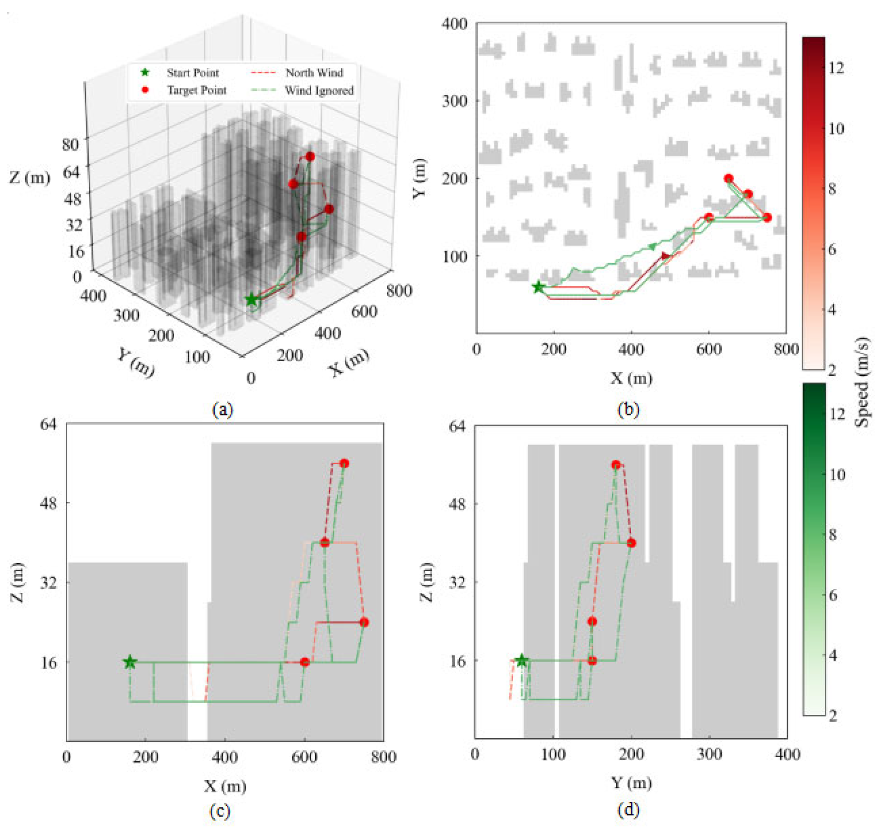
Two test scenarios are designed to evaluate HA*-ACO’s wind-aware path planning performance. The dense delivery scenario features clustered task points causing rapid power fluctuations, with start point (200, 95, 16) and task points at (500, 180, 32), (550, 150, 32), (650, 205, 24), (700, 160, 32), and (750, 190, 24), exhibiting maximum differences of 250 m (x-axis), 45 m (y-axis), and 8 m (z-axis). The multi-layer delivery scenario has significant altitudinal variations leading to higher peak power demands, with start point (160, 60, 16) and task points at (600, 150, 16), (650, 200, 40), (700, 180, 56), and (750, 150, 24), showing a maximum altitude difference of 40 m.

Performance comparison is made against standard ACO without wind consideration. HA*-ACO parameters include: population size 30–100, maximum 200 iterations, 10 initial samples, pheromone importance factor 1–5, heuristic factor 1–5, decay rate 0.1–0.9, weight 0.5, and normalization factor 0.01. Standard ACO uses identical parameter ranges. The computational complexity of the HA*-ACO framework mainly depends on the scale of the voxel search space in the wind-aware A* stage, as well as the ant population size, the number of iterations, and the number of delivery nodes in the ACO stage. Under the parameter settings adopted in this study, the overall computational scale is on the order of $7.2\times 10^5$ basic operations.

Figure 8 and Figure 9 illustrate that the HA*-ACO algorithm generates trajectories with significantly reduced altitude oscillations and fewer abrupt directional changes compared with the wind-agnostic ACO approach. In Scenario 1, the proposed method maintains relatively stable cruising altitudes and avoids unnecessary climb–descent cycles, thereby reducing vertical acceleration demands. In Scenario 2, instead of multiple fragmented altitude adjustments, the HA*-ACO strategy performs a single structured climb followed by a controlled descent.

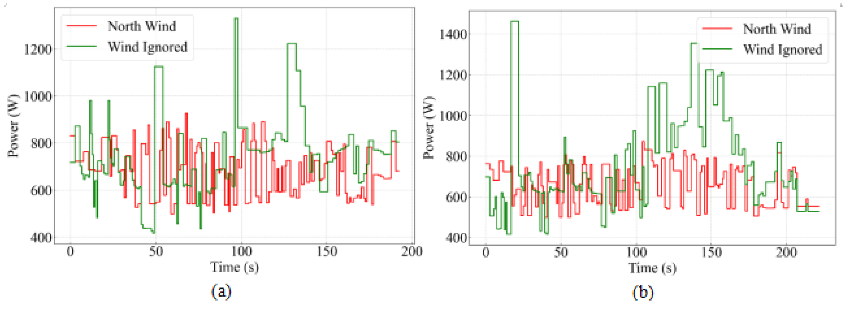
These trajectory characteristics directly influence the power demand profile. Frequent altitude changes and sharp maneuvering typically result in rapid thrust variations and high transient power spikes. By suppressing unnecessary vertical motion and smoothing directional transitions, wind-aware planning produces a more continuous and gradually varying power demand curve. This smoother load profile provides a robust foundation for the subsequent DQN-based energy management strategy.

After obtaining the optimal paths for the UAV under both delivery scenarios, the optimal power curves of the UAV can be derived, which are presented in Figure 10. Scenario 1 has frequent power fluctuations, and Scenario 2 has a greater peak power demand. The erratic trajectory of the standard ACO algorithm results in highly fluctuating power curves, with significant peaks in excess of 1300 W. However, the HA*-ACO path produces a more stable power profile.

Table 1. Energy consumption and distance results in two delivery scenarios.

Scenario ID	Energy (KJ) (Wind Ignored)	Energy (KJ) (North Wind)	Energy Reduction	Distance (m) (Wind Ignored)	Distance (m) (North Wind)	Distance Increase
1	143.74	131.11	8.8%	1222.19	1233.55	0.9%
2	170.03	144.52	15%	1412.11	1451.72	2.8%

quantitatively summarizes the comparative performance between wind-aware HA*-ACO planning and the standard wind-agnostic ACO approach. In Scenario 1 (dense delivery), the proposed HA*-ACO algorithm achieves an 8.8% reduction in total energy consumption while incurring only a marginal 0.9% increase in flight distance. This indicates that minor path length adjustments, when guided by wind-field awareness, can significantly reduce aerodynamic resistance and unnecessary vertical maneuvers, thereby improving overall energy efficiency. In Scenario 2 (multi-layer delivery), the advantage becomes even more pronounced. The proposed method reduces energy consumption by 15%, whereas the flight distance increases by only 2.8%. This demonstrates that, particularly in missions involving substantial altitude variations, incorporating wind effects into trajectory optimization yields considerable energy savings with negligible compromise in mission feasibility. Overall, the results confirm that wind-aware trajectory planning provides a favorable trade-off between energy efficiency and travel distance, making it practically superior to conventional planning strategies that ignore environmental disturbances.

5.2. EMS Results

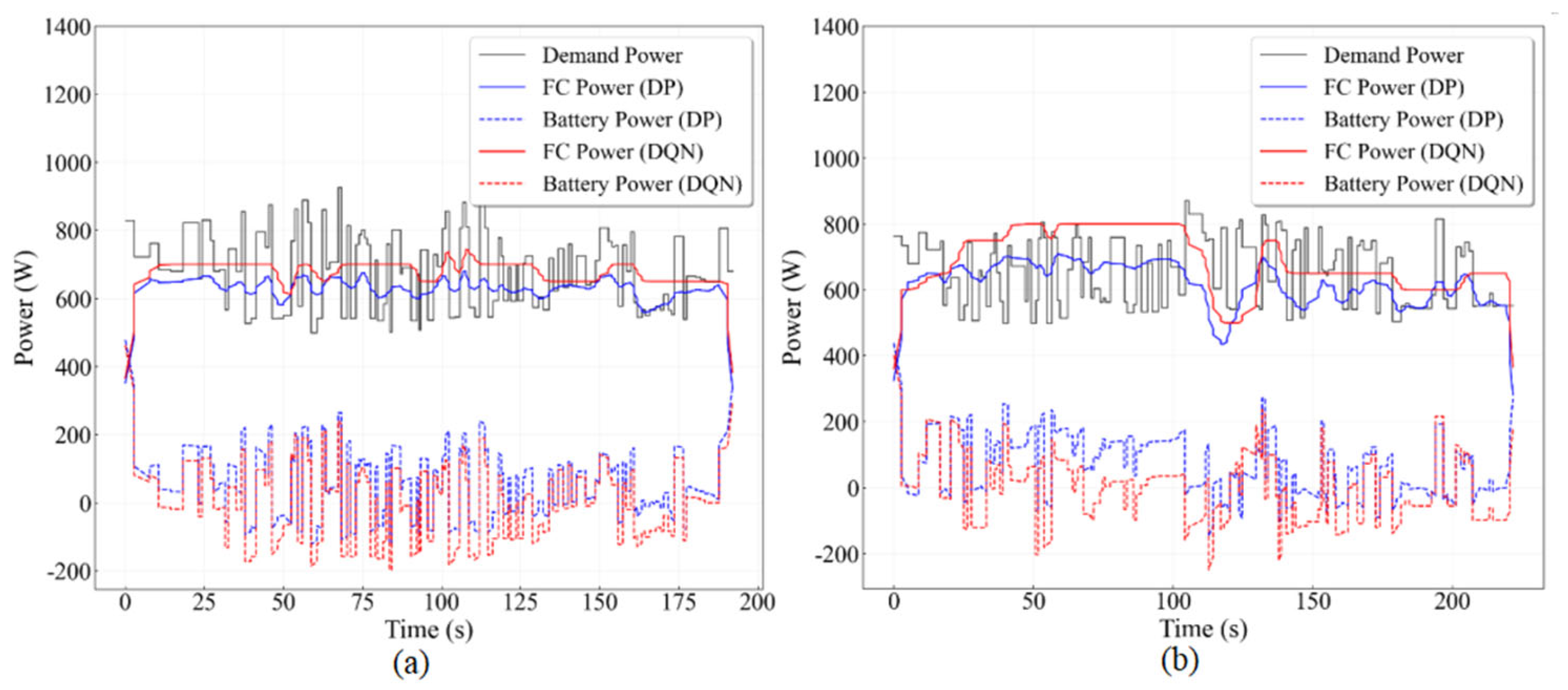
The proposed DQN-based energy management strategy is benchmarked against a hydrogen-consumption-oriented DP approach. In the EMS simulations, the constraint bounds were set as: ${\mathrm{P}}_{\mathrm{f}\mathrm{c}}^{\mathrm{m}\mathrm{a}\mathrm{x}}$ = 1 kW, ${\mathrm{P}}_{\mathrm{b}\mathrm{a}\mathrm{t}}^{\mathrm{m}\mathrm{i}\mathrm{n}}$ = $-600$ W, ${\mathrm{P}}_{\mathrm{b}\mathrm{a}\mathrm{t}}^{\mathrm{m}\mathrm{a}\mathrm{x}}=$ 600 W, $\mathrm{S}\mathrm{O}{\mathrm{C}}^{\mathrm{m}\mathrm{i}\mathrm{n}}$ = 0.2 and $\mathrm{S}\mathrm{O}{\mathrm{C}}^{\mathrm{m}\mathrm{a}\mathrm{x}}$ = 0.8. The DQN agent was trained for 500 epochs with a replay buffer size of 10,000 and a learning rate of 0.001. The training was conducted offline using an NVIDIA RTX 3060 GPU with 32 GB RAM, the total training time was approximately 1.6 h and the sampling interval $\Delta$t was 1s. A smaller time step provides finer control resolution but increases computational cost, whereas a larger time step reduces computational burden at the expense of control precision. Through this iterative interaction-learning process, the agent gradually converged to an effective energy management policy that balances hydrogen consumption, fuel cell power smoothness, and battery SOC regulation. As illustrated in Figure 11, the DQN-based strategy yields a substantially smoother fuel cell power profile than the DP approach. This improvement is particularly evident in the dense delivery scenario during the interval of 75–125 s, where rapid and potentially harmful power fluctuations are effectively mitigated.

In addition, the lithium battery absorbs short-term power variations induced by transient load demands. In the multi-layer delivery scenario, the battery power under the DQN strategy remains within ±200 W during the period of 100–150 s, whereas the DP-based strategy exhibits pronounced and irregular power oscillations. These results demonstrate the superior capability of the DQN-based strategy in smoothing power distribution while accommodating transient power demands.

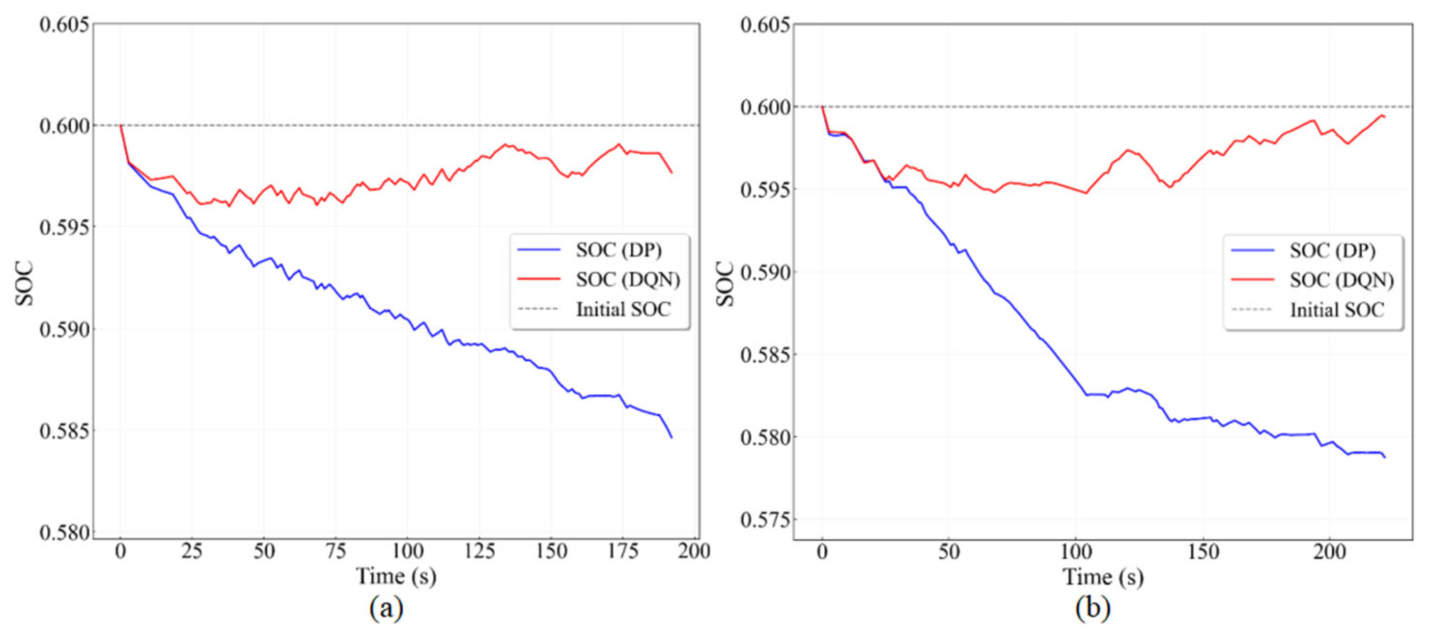
The superior performance of the DQN strategy in maintaining the battery’s SOC is demonstrated in Figure 12. In Scenario 1, the DQN strategy successfully arrests the SOC decline after t = 100 s and initiates a gradual recovery, stabilizing it near the initial 0.600 level. The advantage is even more pronounced in Scenario 2, where the DQN strategy maintains the SOC within a tight band around its initial value. In stark contrast, the DP-based approach, solely focused on minimizing fuel use, leads to a continuous and significant depletion of the SOC in both scenarios. In addition, the DQN-based strategy maintains the battery SOC within a narrow band around its initial level as shown in Figure 12, whereas the DP-based strategy results in continuous SOC depletion. Maintaining SOC within a moderate operating range helps avoid deep discharge and extreme SOC conditions, thereby contributing to extend the battery lifespan.

To further demonstrate the synergy between mission planning and energy management, the performance of the DQN-based strategy is also evaluated on non-optimal flight paths, which are generated using wind-agnostic path planning results. The corresponding quantitative comparison is summarized in

Table 2. EMS performance comparison on the optimal path.

Scenario	Strategy	Demand Power	Hydrogen Consumption (g)	Avg. Power Change (W/s)	Hydrogen Change (%)	Avg. Power Change (%)
Dense delivery	DP	Optimal	1.823	7.54	0%	0%
	DQN	Optimal	1.872	4.69	+2.7%	−37.8%
	DQN	Non-optimal	2.210	5.31	+21.2%	−29.6%
Multi-layer delivery	DP	Optimal	1.990	9.27	0%	0%
	DQN	Optimal	2.093	5.86	+5.2%	−36.8%
	DQN	Non-optimal	2.540	6.77	+27.6%	−27.0%

, which systematically quantifies the trade-offs among the three strategies in terms of hydrogen consumption and fuel cell power fluctuation. While the DP-based strategy marginally excels in minimizing instantaneous hydrogen consumption, the DQN-based strategy achieves near-optimal fuel economy while delivering substantially smoother power allocation. As summarized in Table 2, the DQN strategy reduces the average fuel cell power change rate from 7.54 W/s to 4.69 W/s in Scenario 1, corresponding to a 37.8% reduction relative to the DP benchmark. Similarly, in Scenario 2, the average power change rate achieved by the DQN strategy is reduced to 5.86 W/s, corresponding to a 36.8% decrease compared with the DP strategy’s 9.27 W/s.

In terms of hydrogen consumption, the DQN-based strategy incurs only a modest increase of 2.7% in Scenario 1 and 5.2% in Scenario 2 relative to the DP-based benchmark. In contrast, operating the DQN-based energy management strategy on non-optimal flight paths leads to a pronounced performance degradation. Specifically, in the dense delivery scenario, hydrogen consumption increases by 18.0% (from 1.872 g to 2.210 g), corresponding to an energy increase from approximately 224,640 J to 265,200 J, accompanied by a 13.2% increase in the average power change rate (from 4.69 W/s to 5.31 W/s). A similar deterioration is observed in the multi-layer delivery scenario. These results explicitly demonstrate that optimal path planning not only improves fuel economy but also generates a less aggressive power demand profile, which is essential for enhancing the effectiveness and durability of the hybrid power system.

In conclusion, when compared to a benchmark DP strategy, the DQN-based approach achieves a significant reduction in fuel cell power fluctuations while ensuring robust state-of-charge maintenance for the lithium battery. This is accomplished at the cost of a marginal increase in hydrogen consumption. From a system lifecycle perspective, the DQN strategy presents a more economical choice, as the significant cost of fuel cell replacement far outweighs the minor expense of increased daily hydrogen use. Furthermore, the results prove that an energy management strategy informed by optimal path planning is essential for simultaneously achieving low operational costs and extended system lifespans. From a system lifecycle perspective, the DQN-based strategy represents a more sustainable operational choice. Although it incurs a marginal increase in hydrogen consumption, the substantial reduction in fuel cell power fluctuations significantly lowers long-term degradation rates. Considering that fuel cell stack replacement costs far exceed daily hydrogen expenses, prioritizing power smoothness ultimately leads to improved economic viability and enhanced system durability.

6. Conclusions

This paper targets the urban drone logistics delivery scenario and addresses the critical impact of wind fields on flight performance. It presents an integrated optimization approach that first establishes an energy-efficient flight path considering both energy consumption and distance. Then, based on the resulting power profile, it devises an optimal energy management strategy. This strategy facilitates the entire drone delivery process by optimizing for minimal hydrogen consumption and power fluctuation. The main research contributions and findings are as follows:

Develop the wind-aware UAV power prediction model. To accurately characterize the influence of complex urban wind fields on UAV energy consumption, this study first establishes a high-fidelity three-dimensional wind environment model based on CFD. Leveraging the CFD-simulated wind speed and direction data, a data-driven UAV power prediction framework based on a LSTM network is developed. By jointly incorporating flight kinematic states and localized wind field features, the proposed model is capable of capturing the nonlinear and time-varying coupling between environmental disturbances and power demand. Experimental validation on real flight data demonstrates that the proposed model achieves a root mean square error of 42.99 W and a coefficient of determination of 0.95, confirming its high prediction accuracy and strong generalization capability. This wind-aware power prediction model provides a reliable foundation for both trajectory optimization and subsequent energy management strategy design.

For solving the multi-objective path planning problem under urban wind disturbances, a novel hybrid path planning algorithm, termed HA*-ACO, is proposed. The method integrates a wind-field-aware enhanced A* algorithm for local trajectory optimization with the ACO algorithm for global waypoint sequencing. By explicitly embedding wind-induced energy consumption into the heuristic evaluation, the proposed algorithm generates energy-efficient flight paths that mitigate unnecessary altitude changes and abrupt maneuvers. Simulation results in representative urban delivery scenarios show that the HA*-ACO algorithm reduces total energy consumption by up to 15% compared with wind-agnostic planning methods, while incurring only a marginal increase of 0.9–2.8% in flight distance. These results demonstrate that incorporating wind awareness into trajectory planning is essential for improving energy efficiency without compromising mission feasibility.

Formulate an energy management strategy based on optimal path analysis. Building upon the optimized power demand profiles obtained from wind-aware path planning, this study further develops a DQN-based energy management strategy for a fuel cell–battery hybrid UAV power system. The energy management problem is formulated as a Markov Decision Process, with the objective of minimizing lifecycle operating costs by jointly considering hydrogen consumption, fuel cell power fluctuation, and battery state-of-charge regulation. Compared with a benchmark DP strategy, the proposed DQN-based EMS a achieves a 36.8–37.8% reduction in the average fuel cell power change rate at the cost of only a 2.7–5.2% increase in hydrogen consumption. Moreover, operating the EMS on an optimally planned trajectory enables further performance gains: hydrogen consumption is reduced by up to 17.6%, and power fluctuations are suppressed by up to 13.4% compared with non-optimal paths. These results clearly indicate that trajectory optimization and energy management are strongly coupled, and that optimal path planning plays a critical role in alleviating power stress and extending fuel cell system lifespan.

Overall, the proposed integrated framework demonstrates that trajectory optimization and energy management are strongly coupled through the power demand profile. Wind-aware path planning reshapes the UAV’s velocity and altitude evolution, thereby directly influencing the temporal characteristics of power demand. In turn, the EMS responds to this trajectory-induced load pattern by allocating power between the fuel cell and battery to balance hydrogen consumption and component stress. By jointly optimizing these two stages rather than treating them independently, the proposed framework achieves synergistic improvements in energy efficiency, power smoothness, and component durability. This coupling-aware design provides a practical and effective solution for urban hydrogen-powered UAV logistics.

Future work will extend this framework to multi-UAV cooperative delivery systems, where additional challenges arise in coordinated trajectory planning, real-time conflict resolution, and system-level energy optimization under dynamic mission and environmental uncertainties.

References

1. Jazairy, A.; Persson, E.; Brho, M.; von Haartman, R.; Hilletofth, P. Drones in last-mile delivery: A systematic literature review from a logistics management perspective. Int. J. Logist. Manag. 2025, 36, 1–62. [Google Scholar] [CrossRef]
2. Abdulrahman, A.G.A.Q.; Qasem, N.A.A.; Abdelrahman, W.G.; Alkhulaifi, Y.M.; Almatrafi, E.; Alqahtani, N. A review of powering unmanned aerial vehicles by clean and renewable energy technologies. Sustain. Energy Technol. Assess. 2025, 73, 104150. [Google Scholar] [CrossRef]
3. Kwasiborska, A.; Stelmach, A.; Jabłońska, I. Quantitative and Comparative Analysis of Energy Consumption in Urban Logistics Using Unmanned Aerial Vehicles and Selected Means of Transport. Energies 2023, 16, 6467. [Google Scholar] [CrossRef]
4. Quintana, J.A.; Bordons, C.; Esteban, S.; Delgado, J. Hybrid Powerplant Design and Energy Management for UAVs: Enhancing Autonomy and Reducing Operational Costs. Energies 2025, 18, 3101. [Google Scholar] [CrossRef]
5. Engin, K.O.; Cicek, D.B.; Ozkan, A. A rule-based energy management technique considering altitude energy for a mini UAV with a hybrid power system consisting of battery and solar cell. Energy Convers. Manag. 2023, 287, 117106. [Google Scholar]
6. Lei, Z.; Gu, C.; Li, F.; Zhou, Y.; Yuan, W. An optimal fuzzy logic-based energy management strategy for a fuel cell/battery hybrid power unmanned aerial vehicle. Aerosp. Sci. Technol. 2022, 129, 107821. [Google Scholar]
7. Lee, J.; Yu, B.; Choi, K.; Kim, T. Power management strategy of hybrid fuel cell drones for flight performance improvement based on various algorithms. Energies 2022, 15, 1932. [Google Scholar]
8. Gao, Y.; Qiao, Z.; Pei, X.; Wu, G.; Bai, Y. Design of energy-management strategy for solar-powered UAV. Sustainability 2023, 15, 14972. [Google Scholar] [CrossRef]
9. Liu, H.; Yao, Y.; Wang, J.; Qin, Y.; Li, T. A control architecture to coordinate energy management with trajectory tracking control for fuel cell/battery hybrid unmanned aerial vehicles. Int. J. Hydrogen Energy 2022, 47, 15236–15253. [Google Scholar] [CrossRef]
10. Cheng, Z.; Liu, H.; Yu, P.; Zhu, L.; Sun, T.; Yao, Y. Energy management for fuel cell/battery hybrid unmanned aerial vehicle. Int. J. Electrochem. Sci. 2021, 16, 210919. [Google Scholar] [CrossRef]
11. Tian, W.; Liu, L.; Zhang, X.; Yang, D. Double-layer fuzzy adaptive NMPC coordinated control method of energy management and trajectory tracking for hybrid electric fixed wing UAVs. Int. J. Hydrogen Energy 2022, 47, 39239–39254. [Google Scholar] [CrossRef]
12. Narimanov, J.; Abdujabarov, N. Optimization strategies for energy management systems of solar-powered unmanned aerial vehicles. Acad. Open 2025, 10, 10638. [Google Scholar] [CrossRef]
13. Tian, W.; Liu, L.; Zhang, X.; Shao, J.; Ge, J. Adaptive hierarchical energy management strategy for fuel cell/battery hybrid electric UAVs. Aerosp. Sci. Technol. 2024, 146, 108938. [Google Scholar] [CrossRef]
14. Gao, Q.; Lei, T.; Yao, W.; Zhang, X. A health-aware energy management strategy for fuel cell hybrid electric UAVs based on safe reinforcement learning. Energy 2023, 283, 129092. [Google Scholar] [CrossRef]
15. Chen, Y.; Wang, W.; Yang, C.; Liang, B.; Liu, W. An efficient energy management strategy of a hybrid electric unmanned aerial vehicle considering turboshaft engine speed regulation: A deep reinforcement learning approach. Appl. Energy 2025, 390, 125837. [Google Scholar] [CrossRef]
16. Wang, Z.; Xing, Y. Energy consumption optimisation for unmanned aerial vehicle based on reinforcement learning framework. Int. J. Powertrains 2024, 13, 75–94. [Google Scholar] [CrossRef]
17. Wu, Y.; Low, K.H. An adaptive path replanning method for coordinated operations of drone in dynamic urban environments. IEEE Syst. J. 2021, 15, 4600–4611. [Google Scholar] [CrossRef]
18. Shao, J.; Cheng, J.; Xia, B.; Yang, K.; Wei, H. A novel service system for long-distance drone delivery using the ‘Ant Colony+A*’ algorithm. IEEE Syst. J. 2021, 15, 3348–3359. [Google Scholar] [CrossRef]
19. Manyam, S.G.; Casbeer, D.W.; Darbha, S.; Weintraub, I.E.; Kalyanam, K. Path planning and energy management of hybrid air vehicles for urban air mobility. IEEE Robot. Autom. Lett. 2022, 7, 10176–10183. [Google Scholar] [CrossRef]
20. Tian, W.; Liu, L.; Zhang, X.; Shao, J. Flight trajectory and energy management coupled optimization for hybrid electric UAVs with adaptive sequential convex programming method. Appl. Energy 2024, 364, 123166. [Google Scholar] [CrossRef]
21. Tian, W.; Liu, L.; Zhang, X.; Shao, J.; Ge, J. A coordinated optimization method of energy management and trajectory optimization for hybrid electric UAVs with PV/Fuel Cell/Battery. Int. J. Hydrogen Energy 2024, 50, 1110–1121. [Google Scholar] [CrossRef]
22. Santiago, J.L.; Martilli, A. A dynamic urban canopy parameterization for mesoscale models based on computational fluid dynamics Reynolds-averaged Navier-Stokes microscale simulations. Bound.-Layer Meteorol. 2010, 137, 417–439. [Google Scholar] [CrossRef]
23. Rodrigues, T.A.; Patrikar, J.; Choudhry, A.; Feldgoise, J.; Arcot, V.; Gahlaut, A.; Lau, S.; Moon, B.; Wagner, B.; Matthews, H.S.; et al. In-flight positional and energy use data set of a DJI Matrice 100 quadcopter for small package delivery. Sci. Data 2021, 8, 8. [Google Scholar] [CrossRef]
24. Dorigo, M.; Maniezzo, V.; Colorni, A. Ant system: Optimization by a colony of cooperating agents. IEEE Trans. Syst. Man Cybern. B 1996, 26, 29–41. [Google Scholar] [CrossRef]
25. Beard, R.W.; McLain, T.W. Small Unmanned Aircraft: Theory and Practice; Princeton University Press: Princeton, NJ, USA, 2012. [Google Scholar]
26. Quan, S.; Wang, Y.-X.; Xiao, X.; He, H.; Sun, F. Real-time energy management for fuel cell electric vehicle using speed prediction-based model predictive control considering performance degradation. Appl. Energy 2021, 304, 117845. [Google Scholar] [CrossRef]
Figure 1. Problem illustration.
Energies 19 01854 g001
Figure 2. Schematic diagram of LSTM network architecture.
Energies 19 01854 g002
Figure 3. Power prediction on test set.
Energies 19 01854 g003
Figure 4. Hybrid power system topology. Black solid arrows indicate the main power flow paths in the hybrid power system, while blue dashed arrows indicate the control or signal interactions associated with the EMS controller.
Energies 19 01854 g004
Figure 5. Logical flow of DQN-based EMS.
Energies 19 01854 g005
Figure 6. Local urban voxel obstacle model.
Energies 19 01854 g006
Figure 7. Discrete wind field distribution at various heights under north wind condition: (a) 0–26 m; (b) 27–36 m; (c) 37–60 m; (d) 61–80 m.
Energies 19 01854 g007
Figure 8. Comparison of UAV path planning results in a dense delivery scenario: (a) 3D view; (b) Z-axis projection; (c) X-axis projection; (d) Y-axis projection.
Energies 19 01854 g008
Figure 9. Comparison of UAV path planning results in a multi-layer delivery scenario: (a) 3D view; (b) Z-axis projection; (c) X-axis projection; (d) Y-axis projection.
Energies 19 01854 g009
Figure 10. Comparison of power curves in different scenarios: (a) dense delivery scenario; (b) multi-layer delivery scenario.
Energies 19 01854 g010
Figure 11. Power allocation results for optimal workload based on DP and DQN based strategies for different scenarios: (a) dense delivery scenario; (b) multi-layer delivery scenario.
Energies 19 01854 g011
Figure 12. Comparison of Lithium battery SOC curves for DP and DQN strategies in different scenarios: (a) dense delivery scenario; (b) multi-layer delivery scenario.
Energies 19 01854 g012