Transient Analysis Framework for Heat Pipe Reactors Based on the MOOSE and Its Validation with the KRUSTY Reactor

Abstract

Heat pipe cooled reactors rely on heat pipes for passive heat transfer and exhibit high reliability and compactness. Therefore, they are considered candidate nuclear reactor systems for future deep space exploration missions. To enable a deeper investigation of heat pipe reactor systems, particularly the transient response characteristics of the core, a transient coupled analysis framework is developed based on the multi-physics coupling code MOOSE. This framework includes the core heat transfer module, point kinetics module, heat pipe module, and Stirling engine module. A novel strategy that allows two distinct heat pipe models to be simultaneously invoked within a single simulation in MOOSE is developed. All modules are developed within the MOOSE framework and do not rely on any external programs. The heat pipe module is validated using experimental data from heat pipe startup and operation tests within the maximum relative error of only 0.45%. The entire coupled framework is validated against the KRUSTY operational experiments and is compared with other multi-physics models, demonstrating higher accuracy within the maximum relative error of only 13.7% in core load variation conditions. Meanwhile, transient coupled analyses of the KRUSTY reactor are performed to evaluate its safety performance under accident conditions. In the hypothetical positive reactivity step insertion accident and heat pipe failure accidents, the KRUSTY core exhibits excellent safety performance. And the mechanism of heat pipe power redistribution following heat pipe failure is examined in detail.

1. Introduction

With the advancement of deep space exploration, reliable and high-power density energy systems are required. Space nuclear reactor technology has therefore been developed to meet the demands for safety, reliability, long lifetime, and compactness under launch constraints and extreme space conditions. Among various concepts, the heat pipe cooled reactor (HPR) is considered a promising option. Heat pipes transfer heat through phase change of the working fluid, providing high energy density [1]. Unlike pressurized water reactors, gas-cooled reactors [2], liquid-metal-cooled reactors [3], or molten salt reactors [4], HPRs do not require a circulating coolant, thereby eliminating pumps and reducing the risk of mechanical failure and coolant loss. In addition, such systems exhibit inherent passive safety and reduced cooling system mass [5]. Consequently, heat pipe cooled reactors are regarded as attractive candidates for space applications. Representative designs include SAFE [6], KRUSTY [7], HOMER [8], HP-STMCs [9] and SAIRS [10]. Among them, the KRUSTY has completed a nuclear-fueled operation test, which verified its safety performance under steady-state, transient, and accident conditions [11]. This provides comprehensive and reliable reference data for the numerical simulation of transient analyses.

The transient safety analysis of HPRs involves strong coupling among multiple physical fields, each of which relies on different simulation tools. This interdependence introduces significant difficulties and challenges for numerical simulations. In several studies, such as those conducted by Wu [12], Wang [13], Guo [14], Zhang [15] and Jeong [16], multiple independent simulation programs were employed to solve different physical fields in the coupling analysis of HPRs, and additional programs or scripts were used for data storage and transfer. Simultaneously, Chen [17] conducted a comprehensive multi-physics coupling analysis of a heat pipe molten salt reactor with liquid fuel based on MCNP and Fluent. Compared with a single-program tightly coupled approach, the multi-program external coupling strategy exhibits poorer numerical stability and slower convergence in strongly nonlinear systems with strong feedback effects. The stepwise iterative scheme introduces operator splitting errors and temporal lag errors between physical fields, thereby reducing the accuracy of transient calculations. Furthermore, due to the absence of a fully consistent global Jacobian matrix, nonlinear convergence performance is restricted. Additional interpolation errors and computational overhead are also introduced by data transfer and mesh mapping between different programs.

Other researchers, such as Li [18] and Feng [19], developed an integrated transient analysis code for HPR systems named TAPIRS, which operates independently without relying on any external programs. However, since system analysis programs primarily focus on system-level transient response and overall behavior prediction, their spatial discretization accuracy is inherently limited. High-resolution reconstruction and visualization of three-dimensional field variable distributions are generally not supported, making it difficult to satisfy the requirements for local hot spot analysis and spatial coupling mechanism investigations within the core. A multi-physics coupling framework for HPRs was developed by Chen [20] based on the MOOSE [21], and all physical field modules were integrated to the MOOSE. However, the simplified one-dimensional thermal resistance network model adopted in such work cannot resolve detailed temperature distributions within the heat pipe or provide accurate temperature boundary feedback. In addition, a numerical model for heat pipe frozen startup was not included, and therefore, the cold startup process of a HPR cannot be simulated within that framework. Furthermore, an energy conversion system was also not incorporated into the overall coupling framework.

Therefore, based on the current state of research, a multi-physics coupling framework for HPRs is developed in this work using MOOSE. All physical models are implemented and integrated entirely within MOOSE. The framework supports the thermal resistance network model and the closed-form analytical solution model being invoked simultaneously within a single calculation, and it can simulate the reactor core from cold startup to steady-state operation. Furthermore, various accident scenarios of KRUSTY are investigated through transient simulations based on this framework. In particular, heat pipe failure accidents were analyzed, and the mechanism of heat pipe power redistribution following heat pipe failure was examined in detail.

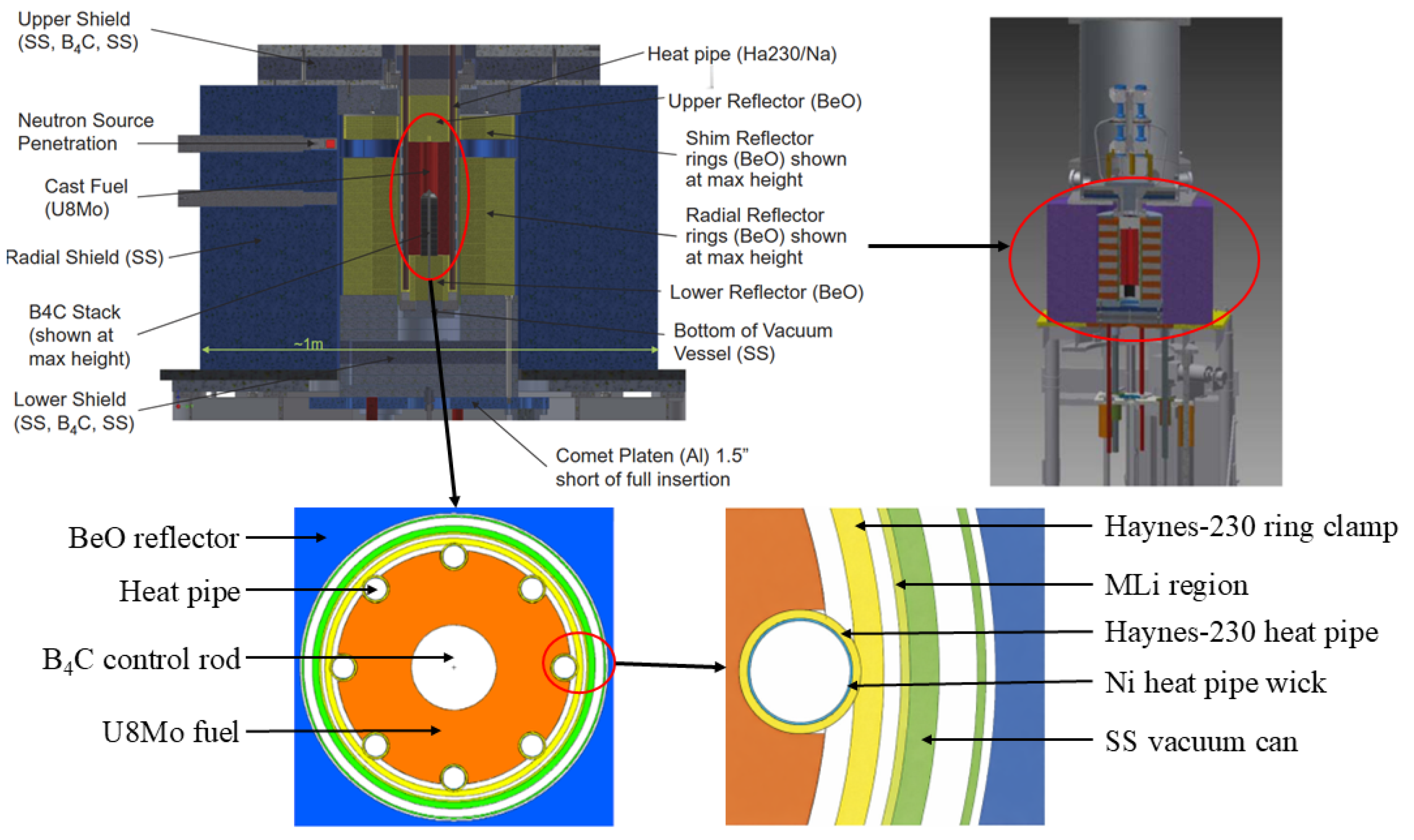
The structural schematic of the KRUSTY reactor (Los Alamos National Laboratory and NASA, Los Alamos, NM, USA) is shown in Figure 1. The KRUSTY reactor features a highly simplified configuration, consisting of a cylindrical U8Mo fuel element surrounded by eight heat pipes, each coupled to a single Stirling engine for heat removal [22]. The core is surrounded by a movable BeO reflector, with a control rod channel positioned at its center.

This paper is structured as follows: In Section 2, five theoretical models and their implementations within the MOOSE framework are described in detail, and the coupling calculations among the multiple physical fields are also presented. In Section 3, both heat pipe models are validated with experimental data obtained from heat pipe startup and normal operation tests. By utilizing the powerful mesh generation capability of the MOOSE framework, the transient analyses of the KRUSTY is simulated in three dimensions and validated with experimental data. And the safety performance of the KRUSTY and its heat pipes under accident conditions is evaluated. In Section 4, the work presented in this study is summarized, and perspectives for future research are provided based on the developed model.

2. Theoretical Models and Framework

In this section, a MOOSE-based mathematical framework for the transient analysis of heat pipe reactors is established. The computational framework integrates heat transfer, point kinetics, heat pipe, and Stirling engine modules. The overall transient calculation process and multi-physics coupling strategy are also illustrated.

2.1. Core Heat Transfer Module

The Heat Conduction Module in MOOSE is used to analyze the heat transfer behavior of the core in this work. The heat conduction equation used in this module can be expressed as

$$\begin{array}{c}\hfill \begin{array}{c}\hfill \rho (t,\overrightarrow{x})c(t,\overrightarrow{x}){\displaystyle \frac{\partial T}{\partial t}}=\nabla k(t,\overrightarrow{x})\nabla T+q\end{array}\end{array}$$

(1)

where $\rho$, $c_p$, k and q are density, heat capacity, thermal conductivity and heat source respectively. The heat source term q is specified through the ICs module in MOOSE.

2.2. Point Kinetics Module

The time-dependent variation in the core fission power is calculated using the point kinetics equations. This module is implemented by customizing the ScalarKernel class in MOOSE. Owing to the compact geometry of the KRUSTY core and its characteristic fast neutron spectrum, the point kinetics approach is well-suited for this analysis.

$$\begin{array}{c}\hfill \begin{array}{c}\hfill {\displaystyle \frac{\mathrm{d}P\left(t\right)}{\mathrm{d}t}}={\displaystyle \frac{\rho \left(t\right)-\beta }{\Lambda }}P\left(t\right)+\sum _{i=1}^6{\lambda }_i{C}_i\left(t\right),\beta =\sum _1^6{\beta }_i\end{array}\end{array}$$

(2)

$$\begin{array}{c}\hfill \begin{array}{c}\hfill {\displaystyle \frac{\mathrm{d}{C}_i\left(t\right)}{\mathrm{d}t}}={\displaystyle \frac{{\beta }_i}{\Lambda }}P\left(t\right)-{\lambda }_i{C}_i\left(t\right),i=1,2,3,\dots ,6\end{array}\end{array}$$

(3)

$$\begin{array}{c}\hfill \begin{array}{c}\hfill \rho \left(t\right)={\rho }_0+{\rho }_{ex}+{\alpha }_{fuel}(T_{fuel}\left(t\right)-T_{fuel,0})+{\alpha }_{hp}(T_{hp}\left(t\right)-T_{hp,0})\end{array}\end{array}$$

(4)

where $\mathit{P}$, ${\beta }_i$, $C_i$, ${\lambda }_i$ and $\Lambda$ are the fission power, the delayed neutron fraction, concentration of delayed neutron precursors, the decay constant of delayed neutron and the neutron generation time, respectively; $\rho$ is the total reactivity, ${\rho }_0$ is the initial reactivity, ${\rho }_{ex}$ is the externally introduced reactivity, ${\alpha }_{fuel}$ is the fuel temperature reactivity coefficient, and ${\alpha }_{hp}$ is the total heat pipe temperature reactivity coefficient.

2.3. Heat Pipe Model

2.3.1. Thermal Resistance Network

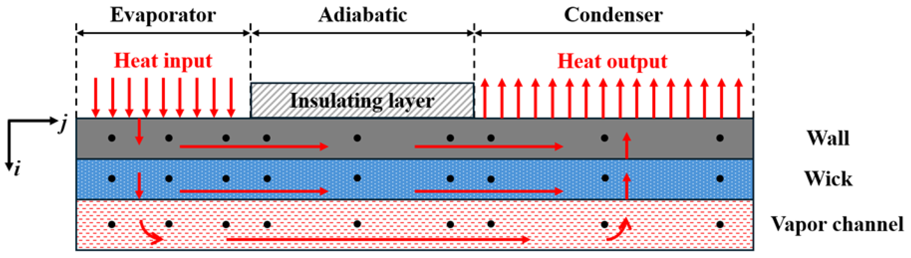
The normal operating state of heat pipes is typically analyzed using thermal resistance network models. In this work, as shown in Figure 2, an improved thermal resistance network model for heat pipes is developed, building upon the models proposed by Yuchuan Guo [24] and Ziang Guo [25]. In this model, the heat pipe is discretized into multiple nodes along both the radial and axial directions, with the number of nodes determined by the actual length of the heat pipe and the required computational accuracy.

The heat pipe wall is axially divided into three regions, namely the evaporator, the adiabatic, and the condenser section, with each region discretized into multiple nodes. The multi-node representation of the evaporator allows for non-uniform power input.

The governing equation for the evaporator section can be expressed as

$$\begin{array}{c}\hfill \begin{array}{c}\hfill {\rho }_{(i,j)}{C}_{(i,j)}{\displaystyle \frac{d{T}_{(i,j)}}{dt}}=Q_{hp(i,j)}+{\displaystyle \frac{T_{(i+1,j)}-T_{(i,j)}}{R_{(i+1,j)(i,j)}}}+{\displaystyle \frac{T_{(i,j-1)}-T_{(i,j)}}{R_{(i,j-1)(i,j)}}}+{\displaystyle \frac{T_{(i,j+1)}-T_{(i,j)}}{R_{(i,j+1)(i,j)}}}\end{array}\end{array}$$

(5)

In this model, the external heat loss from the wall of the adiabatic section in the radial direction is neglected. Therefore, the governing equation for the adiabatic section can be expressed as

$$\begin{array}{c}\hfill \begin{array}{c}\hfill {\rho }_{(i,j)}{C}_{(i,j)}{\displaystyle \frac{d{T}_{(i,j)}}{dt}}={\displaystyle \frac{T_{(i+1,j)}-T_{(i,j)}}{R_{(i+1,j)(i,j)}}}+{\displaystyle \frac{T_{(i,j-1)}-T_{(i,j)}}{R_{(i,j-1)(i,j)}}}+{\displaystyle \frac{T_{(i,j+1)}-T_{(i,j)}}{R_{(i,j+1)(i,j)}}}\end{array}\end{array}$$

(6)

The governing equation for the condenser section can be expressed as

$$\begin{array}{c}\hfill \begin{array}{c}\hfill {\rho }_{(i,j)}{C}_{(i,j)}{\displaystyle \frac{d{T}_{(i,j)}}{dt}}={\displaystyle \frac{T_{(i+1,j)}-T_{(i,j)}}{R_{(i+1,j)(i,j)}}}+{\displaystyle \frac{T_{(i,j-1)}-T_{(i,j)}}{R_{(i,j-1)(i,j)}}}+{\displaystyle \frac{T_{(i,j+1)}-T_{(i,j)}}{R_{(i,j+1)(i,j)}}}+{\displaystyle \frac{T_{\left(j\right)f}-T_{(i,j)}}{R_{\left(j\right)f(i,j)}}}\end{array}\end{array}$$

(7)

The governing equation for transient heat transfer in the wick region is as follows:

$$\begin{array}{c}\hfill \begin{array}{c}\hfill {\rho }_{(i,j)}{c}_{p(i,j)}{V}_{(i,j)}{\displaystyle \frac{d{T}_{(i,j)}}{dt}}={\displaystyle \frac{T_{(i+1,j)}-T_{(i,j)}}{R_{(i+1,j)(i,j)}}}+{\displaystyle \frac{T_{(i-1,j)}-T_{(i,j)}}{R_{(i-1,j)(i,j)}}}+{\displaystyle \frac{T_{(i,j-1)}-T_{(i,j)}}{R_{(i,j-1)(i,j)}}}+{\displaystyle \frac{T_{(i,j+1)}-T_{(i,j)}}{R_{(i,j+1)(i,j)}}}\end{array}\end{array}$$

(8)

Due to the unique structure of the heat pipe wick region, its density, specific heat capacity, and thermal conductivity are evaluated based on porous media theory. The corresponding equivalent equations are as follows:

$$\begin{array}{c}\hfill \begin{array}{c}\hfill {\rho }_{(i,j)}=\phi {\rho }_l+(1-\phi ){\rho }_w\end{array}\end{array}$$

(9)

$$\begin{array}{c}\hfill \begin{array}{c}\hfill c_{p(i,j)}=\phi c_{pl}+(1-\phi )c_{pw}\end{array}\end{array}$$

(10)

$$\begin{array}{c}\hfill \begin{array}{c}\hfill {\lambda }_{(i,j)}={\lambda }_l{\displaystyle \frac{({\lambda }_l+{\lambda }_w)-(1-\phi )({\lambda }_l-{\lambda }_w)}{({\lambda }_l+{\lambda }_w)+(1-\phi )({\lambda }_l-{\lambda }_w)}}\end{array}\end{array}$$

(11)

The transient heat transfer governing equation for the vapor region of the heat pipe is given in Equation (12). This equation is applicable only after the heat pipe has been fully activated and continuous vapor flow has been established.

$$\begin{array}{c}\hfill \begin{array}{c}\hfill {\rho }_{(i,j)}{C}_{(i,j)}{V}_{(i,j)}{\displaystyle \frac{d{T}_{(i,j)}}{dt}}={\displaystyle \frac{T_{(i-1,j)}-T_{(i,j)}}{R_{(i-1,j)(i,j)}}}+{\displaystyle \frac{T_{(i,j-1)}-T_{(i,j)}}{R_{(i,j-1)(i,j)}}}+{\displaystyle \frac{T_{(i,j+1)}-T_{(i,j)}}{R_{(i,j+1)(i,j)}}}\end{array}\end{array}$$

(12)

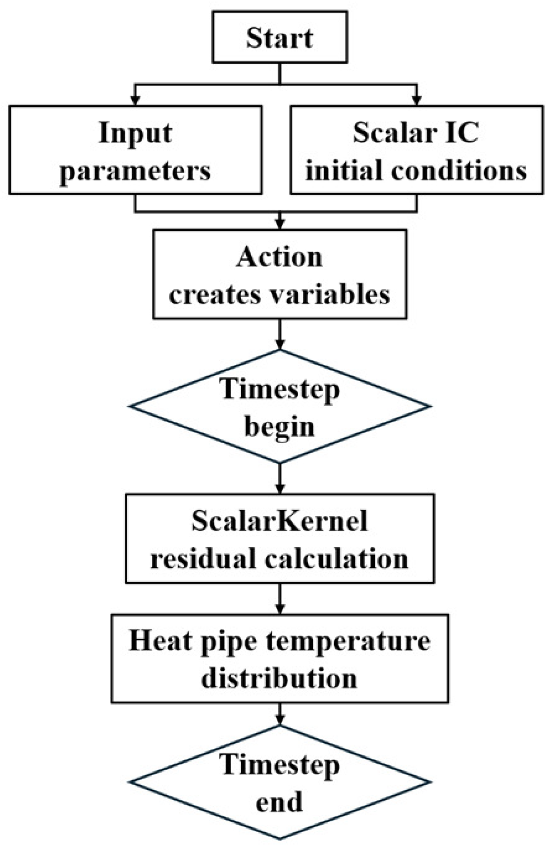
The above model is implemented by rewriting the ScalarIC, ScalarKernel, and Action classes in MOOSE. The detailed implementation process is illustrated in Figure 3. The Action creates scalar variables and couples them with the ScalarKernel for residual calculation of the governing equations and the ScalarIC for inputting variables’ initial conditions.

2.3.2. Frozen Startup

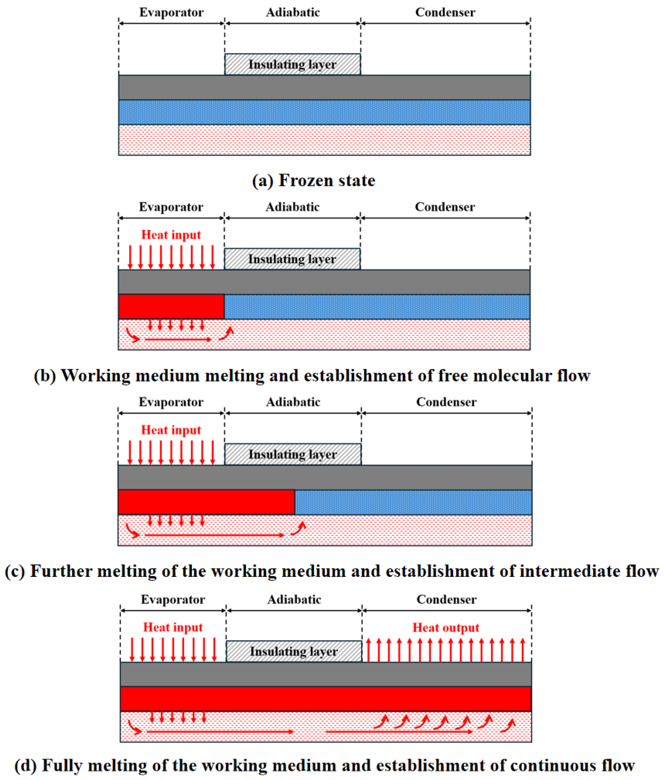
Frozen startup of high-temperature alkali metal heat pipes involves complex multi-physics coupling and phase-change processes, as illustrated in Figure 4. In this work, an approximate closed-form analytical solution [26] is employed to determine the hot zone length and temperature distribution during the heat pipe startup phase. For l = $L_e$, the relation between the startup time and the average hot zone temperature is

$$\begin{array}{c}\hfill \begin{array}{c}\hfill t={\displaystyle \frac{Q{L}_e}{\left[C(T_{aw}-T_a)\right]}}\end{array}\end{array}$$

(13)

For $L_e$ < l < ($L_e$+$L_a$) and l≥ ($L_e$+$L_a$), Equations (14) and (15) should be used to calculate the hot zone length, respectively.

$$\begin{array}{}\mathrm{(14)}& l={\displaystyle \frac{Qt}{\left[C(T_{aw}-T_a)\right]}}\hfill & l=\left[{\displaystyle \frac{Q}{(T_{aw}-T_a)2\pi R_{w}h}}+(L_e+L_a)\right]+\left[1-exp\left[-{\displaystyle \frac{2\pi R_{w}h(t-t_i)}{C}}\right]\right]\hfill \mathrm{(15)}& +{\displaystyle \frac{(L_e+L_a)(T_{aw,i}-T_a)}{(T_{aw}-T_a)}}exp\left[-{\displaystyle \frac{2\pi R_{w}h(t-t_i)}{C}}\right]\hfill \end{array}$$

where $T_{aw,i}$ and $t_i$ represent the wall temperature and time when the planar front reaches the condenser inlet, respectively. The vapor flow inside the heat pipe is assumed to be incompressible, the axial pressure drop and temperature drop along the heat pipe can be expressed as

$$\begin{array}{c}\hfill \begin{array}{c}\hfill \Delta p={\displaystyle \frac{4\mu Ql}{\pi {\rho }_v{R}_v^4{h}_{fg}}}\end{array}\end{array}$$

(16)

$$\begin{array}{c}\hfill \begin{array}{c}\hfill \Delta T={\left({\displaystyle \frac{T}{{\rho }_v{h}_{fg}}}\right)}_{av}\Delta p\end{array}\end{array}$$

(17)

Considering vapor compressibility and density variations, the average vapor density should be related to the mean vapor temperature. Based on the ideal gas law and the integral form of the Clausius–Clapeyron equation, the following expression can be obtained:

$$\begin{array}{c}\hfill \begin{array}{c}\hfill {\rho }_v={\displaystyle \frac{1}{R{T}_{av}}}{p}_{rf}exp\left[-{\displaystyle \frac{h_{fg}}{R}}({\displaystyle \frac{1}{T_{av}}}-{\displaystyle \frac{1}{T_{rf}}})\right]\end{array}\end{array}$$

(18)

where $p_{rf}$ and $T_{rf}$ represent the saturation reference pressure and temperature. According to the assumption of a linear hot zone temperature distribution and the neglection of the radial temperature drop across the wall and wick, we have

$$\begin{array}{c}\hfill \begin{array}{c}\hfill T_{av}=T_{aw}=0.5(T_h+T_{tr})=T_{tr}+0.5\Delta T\end{array}\end{array}$$

(19)

Combining Equations (18) and (19), we can obtain

$$\begin{array}{c}\hfill \begin{array}{c}\hfill {\displaystyle \frac{h_{fg}}{R}}\left({\displaystyle \frac{1}{T_{rf}}}-{\displaystyle \frac{1}{T_{tr}+0.5\Delta T}}\right)-ln\left[{\displaystyle \frac{R(T_{rf}+0.5\Delta T)}{p_{rf}}}{\left({\displaystyle \frac{4(T_{rf}+0.5\Delta T)\mu Ql}{\pi \Delta T{R}_v^4{h}_{fg}}}\right)}^{0.5}\right]=0\end{array}\end{array}$$

(20)

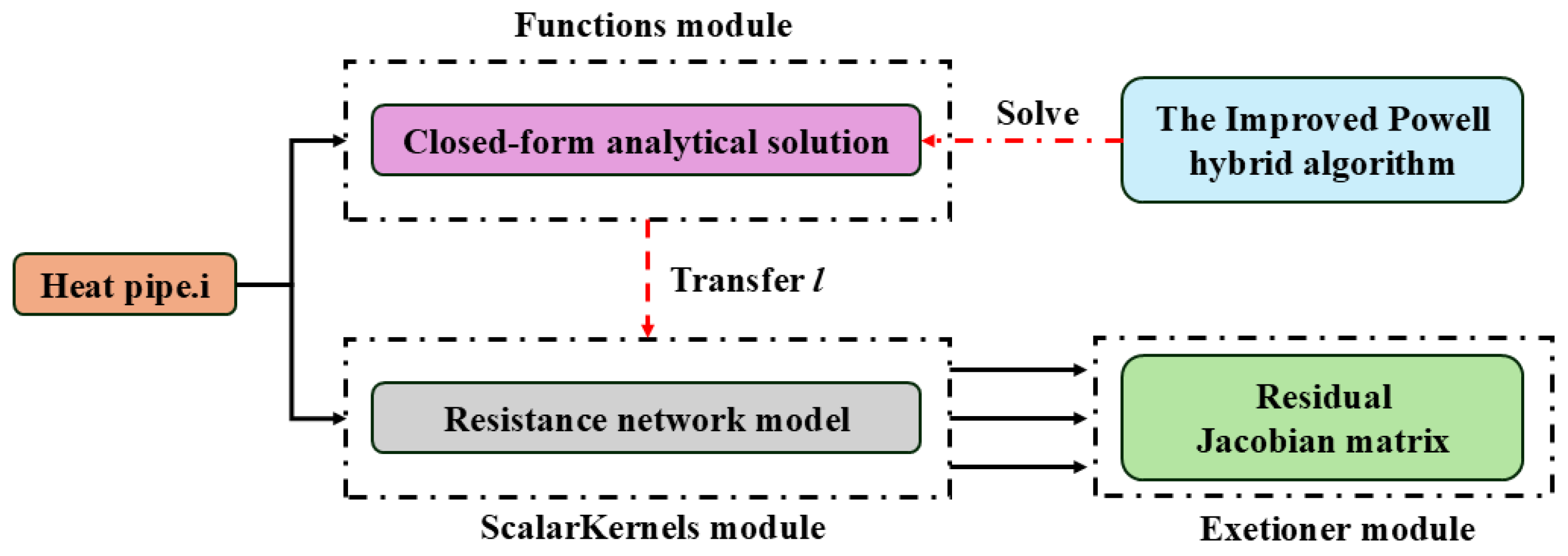
As shown in Figure 5, the closed-form analytical solution model is constructed based on the Functions module in MOOSE, and the Improved Powell hybrid algorithm is embedded in the source code for its solution. In contrast, the thermal resistance network model relies on the ScalarKernels module and is solved using the solver specified in the input file. The Functions module does not participate in residual evaluation or Jacobian matrix construction. Therefore, even when the two modules are invoked simultaneously, numerical errors are not introduced. The closed-form analytical solution model only transfers the hot zone length to the thermal resistance network model to determine thermal resistance parameters. After the heat pipe is fully started, the closed-form analytical solution model no longer participates in the calculation, and the thermal resistance network model continues the subsequent computation based on the last updated hot zone length. This demonstrates that the heat pipe model developed in this work is fully capable of simulating the transient process from cold startup to steady-state operation within a single calculation.

2.4. Stirling Model

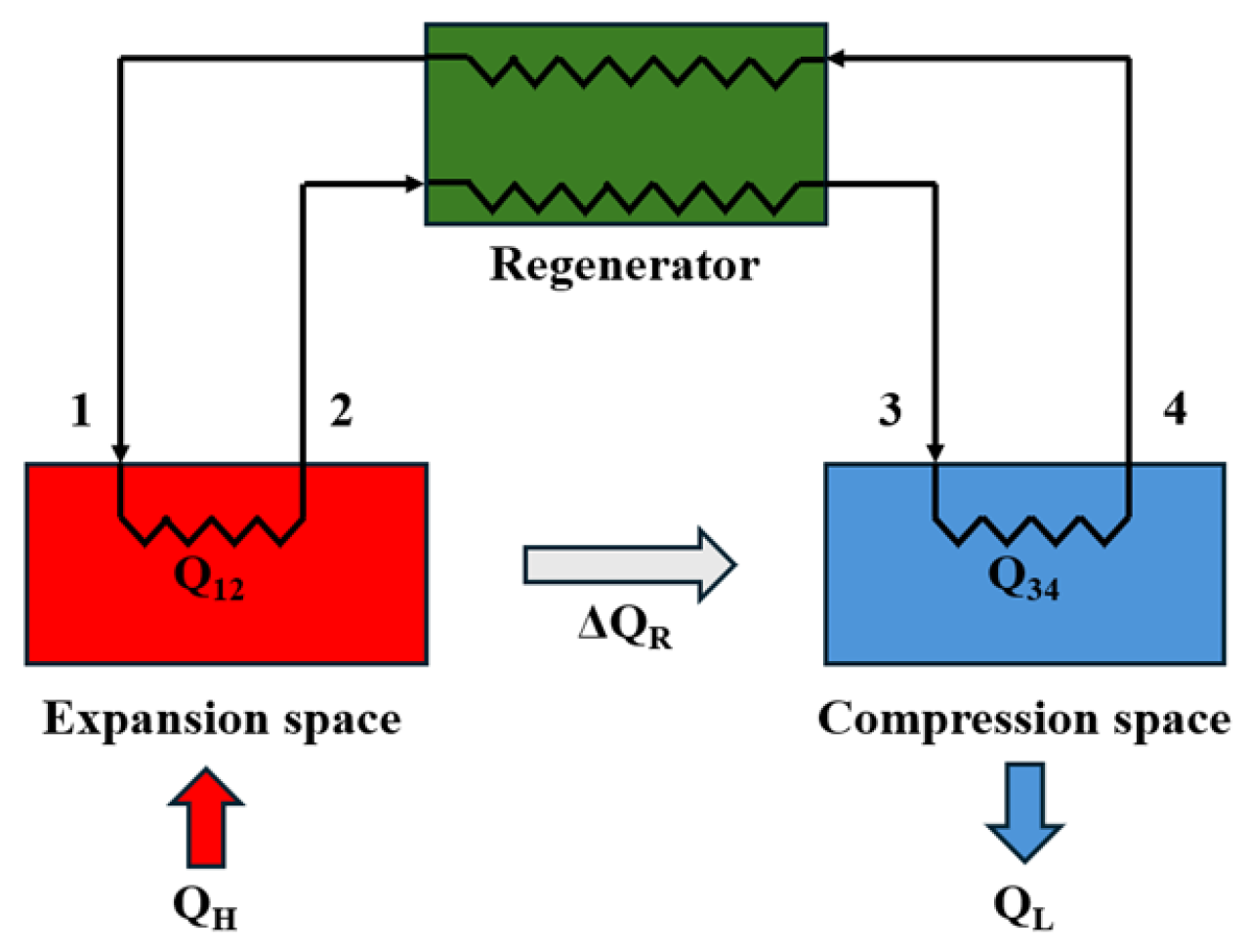
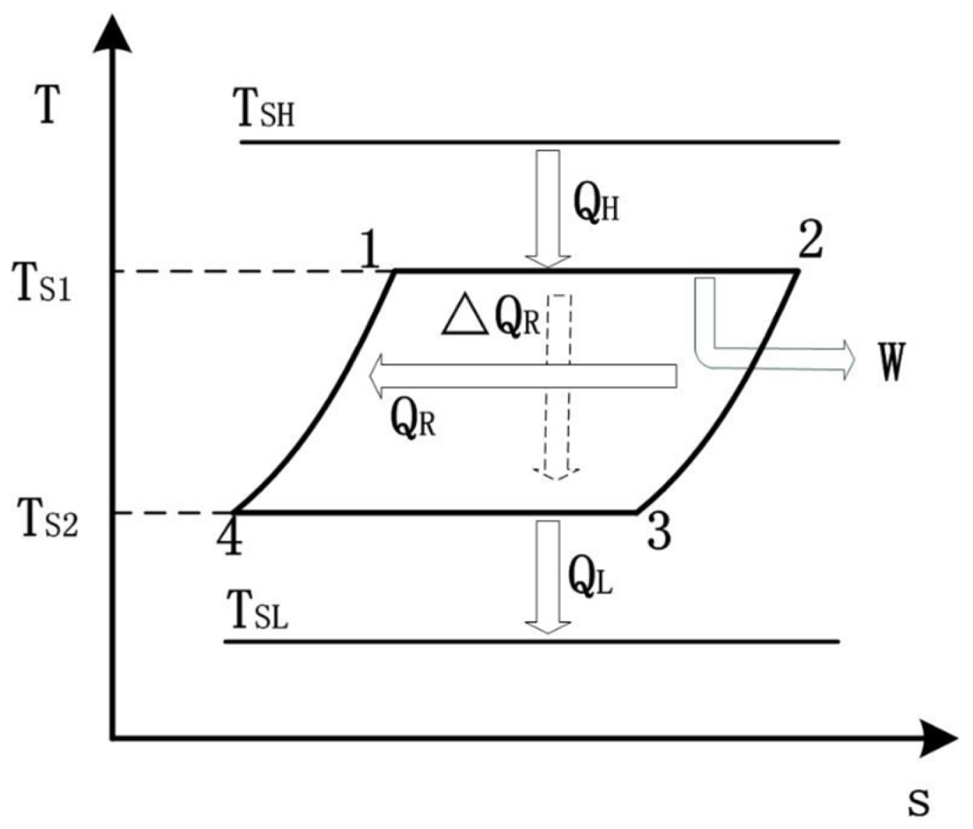
Since the thermal inertia and mechanical response time of the Stirling engine are typically on the order of microseconds or milliseconds, they are negligible compared with the thermal inertia of the core and heat pipes. In addition, the present work primarily focuses on the power and temperature variations of the core and heat pipes, while the thermal response behavior of the Stirling engine is of secondary importance. Therefore, a simplified quasi-steady-state Stirling model was adopted for the simulations. The simplified model [27] and the cycle T–S diagram of the Stirling engine are shown in Figure 6 and Figure 7. The engine mainly consists of a hot end, a cold end, a regenerator and a piston assembly. Power output is achieved through the pressure variation of the working gas at different temperatures. The Stirling cycle mainly consists of the following four processes: (1) Isothermal expansion (1–2): The working fluid is heated at the hot end and expands while causing the piston to move, with its temperature remaining constant. (2) Isochoric cooling (2–3): The working fluid releases some heat to the regenerator at a constant volume. (3) Isothermal compression (3–4): The working fluid is compressed and releases heat to the cold end while maintaining a constant temperature. (4) Isochoric heating (4–1): The working fluid is heated at the regenerator while keeping a constant volume.

Assuming the working fluid is an ideal gas and that the amount of substance in the engine is n moles, the heat absorbed $Q_{12}$ during processes 1–2 and the heat rejected $Q_{34}$ during processes 3–4 are given by

$$\begin{array}{c}\hfill \begin{array}{c}\hfill Q_{12}=nR{T}_{S1}lnCR\end{array}\end{array}$$

(21)

$$\begin{array}{c}\hfill \begin{array}{c}\hfill Q_{34}=nR{T}_{S2}lnCR\end{array}\end{array}$$

(22)

where CR = $V_2$/$V_1$ is the compression ratio, $V_1$ denotes the initial volume at the beginning of the isothermal expansion process, and $V_2$ represents the volume at the end of the process. The regenerative loss caused by incomplete regeneration is given as

$$\begin{array}{c}\hfill \begin{array}{c}\hfill \Delta Q_R=n{c}_v(1-{\eta }_R)(T_{S1}-T_{S2})\end{array}\end{array}$$

(23)

where $c_v$ is the molar specific heat at a constant volume of the working fluid, and ${\eta }_R$ is the efficiency of the regenerator. Thus, the actual heat exchange between the working fluid and the high- and low-temperature heat sources per cycle, $Q_H$ and $Q_L$, can be expressed as

$$\begin{array}{c}\hfill \begin{array}{c}\hfill Q_H=nR{T}_{S1}lnCR+n{c}_v(1-{\eta }_R)(T_{S1}-T_{S2})\end{array}\end{array}$$

(24)

$$\begin{array}{c}\hfill \begin{array}{c}\hfill Q_L=nR{T}_{S2}lnCR+n{c}_v(1-{\eta }_R)(T_{S1}-T_{S2})\end{array}\end{array}$$

(25)

Therefore, the cycle period can be expressed as

$$\begin{array}{cc}\hfill & t_s=t_{1-2}+t_{2-3}+t_{3-4}+t_{4-1}\hfill \\ & ={\displaystyle \frac{nR{T}_{S1}lnCR+n{c}_v(1-{\eta }_R)(T_{S1}-T_{S2})}{{\left(KA\right)}_H(T_{SH}-T_{S1})}}\hfill \\ \hfill & +{\displaystyle \frac{nR{T}_{S2}lnCR+n{c}_v(1-{\eta }_R)(T_{S1}-T_{S2})}{{\left(KA\right)}_L(T_{S2}-T_{SL})}}+{\displaystyle \frac{2(T_{S1}-T_{S2})}{\beta }}\hfill \end{array}$$

(26)

where ${\left(KA\right)}_H$ and ${\left(KA\right)}_L$ represent the products of the heat transfer area and the thermal conductivity for the high- and low-temperature heat sources, respectively, and $\beta$ denotes the time constant of the regenerator.

Therefore, the output power and efficiency of the system can be expressed as [18]

$$\begin{array}{c}\hfill \begin{array}{c}\hfill P_s={\displaystyle \frac{Q_H-Q_L}{t_s}}={\displaystyle \frac{nR(T_{S1}-T_{S2})lnCR}{t_s}}\end{array}\end{array}$$

(27)

$$\begin{array}{c}\hfill \begin{array}{c}\hfill {\eta }_s={\displaystyle \frac{Q_H-Q_L}{Q_H}}={\displaystyle \frac{R(T_{S1}-T_{S2})lnCR}{R{T}_{S1}lnCR+c_v(1-{\eta }_R)(T_{S1}-T_{S2})}}\end{array}\end{array}$$

(28)

2.5. Calculation Procedure and Coupling Method

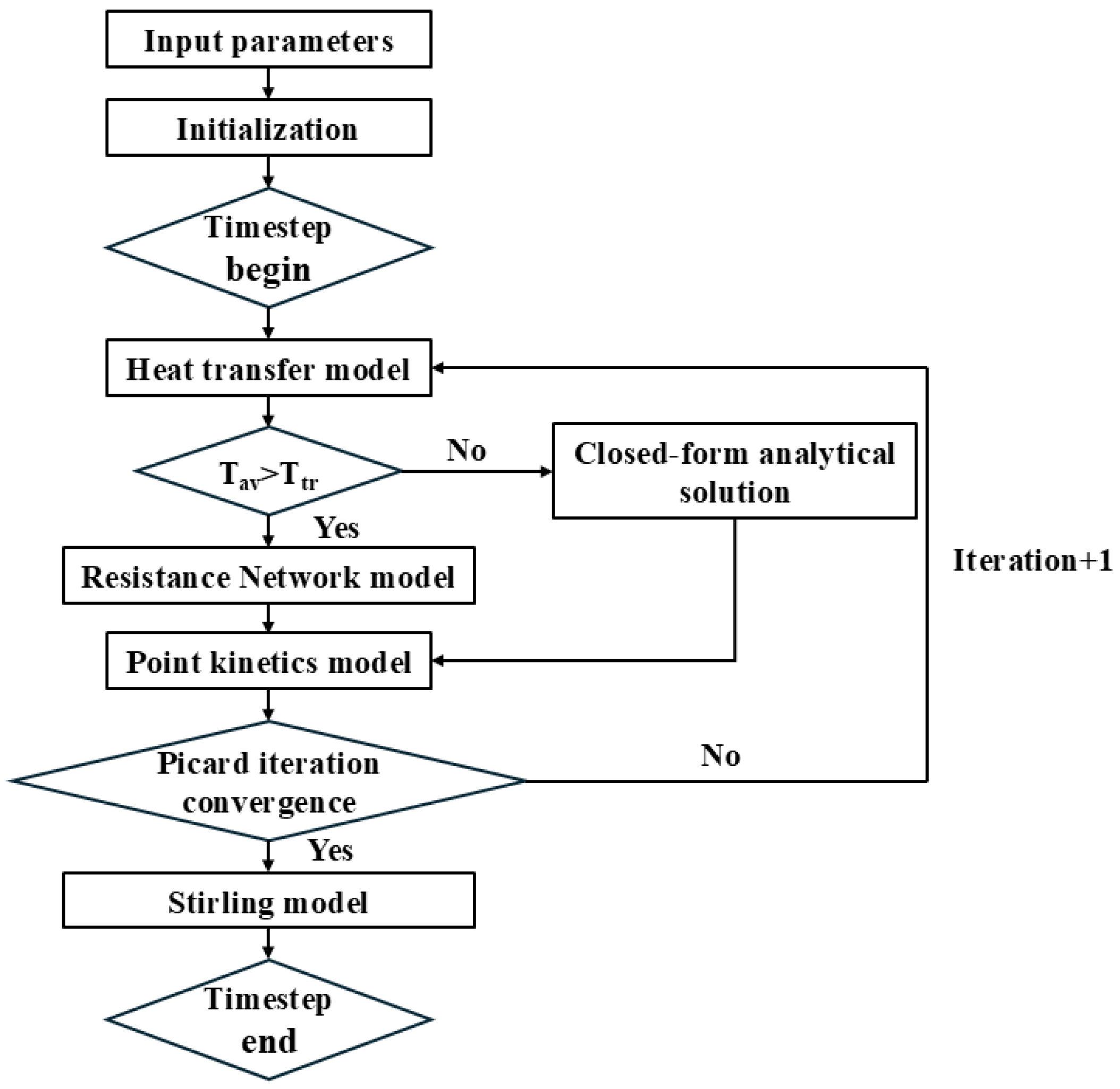
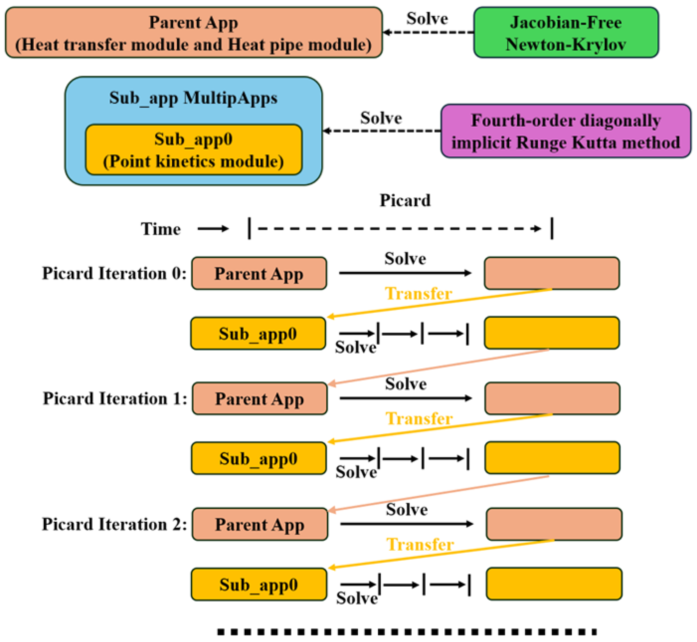
All modules are implemented within the MOOSE framework and do not rely on any external programs. Interactions and data exchanges among modules are achieved by MultiApps and Transfer modules. The overall transient calculation procedure is shown in Figure 8. The heat transfer and heat pipe modules are tightly coupled and are solved using JFNK executioner. After the heat transfer calculations are completed, the temperature field is loosely coupled to the point kinetics module through the Picard iteration method [28]. The Picard iteration process implemented in MOOSE is illustrated in Figure 9. Owing to the stiffness of the point kinetics equations, a small time step is required. To improve computational efficiency, the sub-cycling feature in MOOSE is adopted in which the point kinetics module uses a time step of 0.01 s, while the heat transfer and heat pipe modules use a time step of 0.1 s.

3. Results and Discussion

In this section, the established heat pipe model and transient analysis framework are validated. Such framework is applied to simulate the KRUSTY reactor, with particular focus on several representative safety scenarios, including reactivity insertion accidents and heat pipe failure accidents.

3.1. Heat Pipe Model Validation

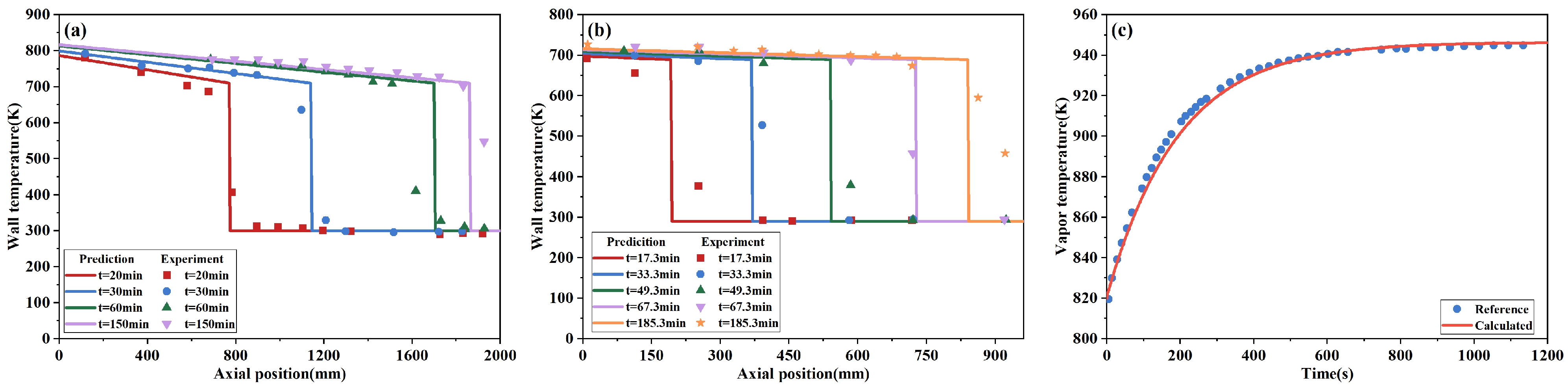
The heat pipe frozen startup module developed in this work is validated through comparison with sodium heat pipe experiments conducted by Faghri [29] and Ponnappan [30]. The key parameters of the experimental heat pipes are listed in

Table 1. Parameters of the sodium heat pipe experiment.

Parameter	Fagrhi	Ponnappan	Cao
Evaporator section length/mm	53	375	105
Adiabatic section length/mm	617	745	52.5
Condenser section length/mm	292	910	542.5
Heat pipe outer diameter/mm	26.7	22.2	16
Heat pipe wall thickness/mm	2.15	1.65	1
Vapor core radius/mm	21.5	12.7	14
Ambient temperature/K	290	298	300
Qin/W	119	289.6	623→770

. The simulation results are shown in Figure 10a,b, and good agreement is observed between the simulations and the experimental data, although relatively large temperature deviations appear in the discontinuous regions of the heat pipe. This is due to the original analytical model in which the temperature in the discontinuous regions is assumed to be room temperature.But axial heat conduction within the heat pipe also causes a temperature rise in discontinuous regions. However, the temperature distribution of the heat pipe obtained from the simulation is sufficiently accurate for coupled calculations between the heat pipe and the reactor core.

The thermal resistance network method is validated with the sodium heat pipe case by Cao and Faghri [31]. In this case, a transient process is simulated in which the input power of the heat pipe increased from 623 W to 770 W. The comparison between the simulation results and the reference data is presented in Figure 10c, showing a maximum relative error of only 0.45%, which demonstrates the accuracy of the model.

3.2. Validation with the KRUSTY Experiment

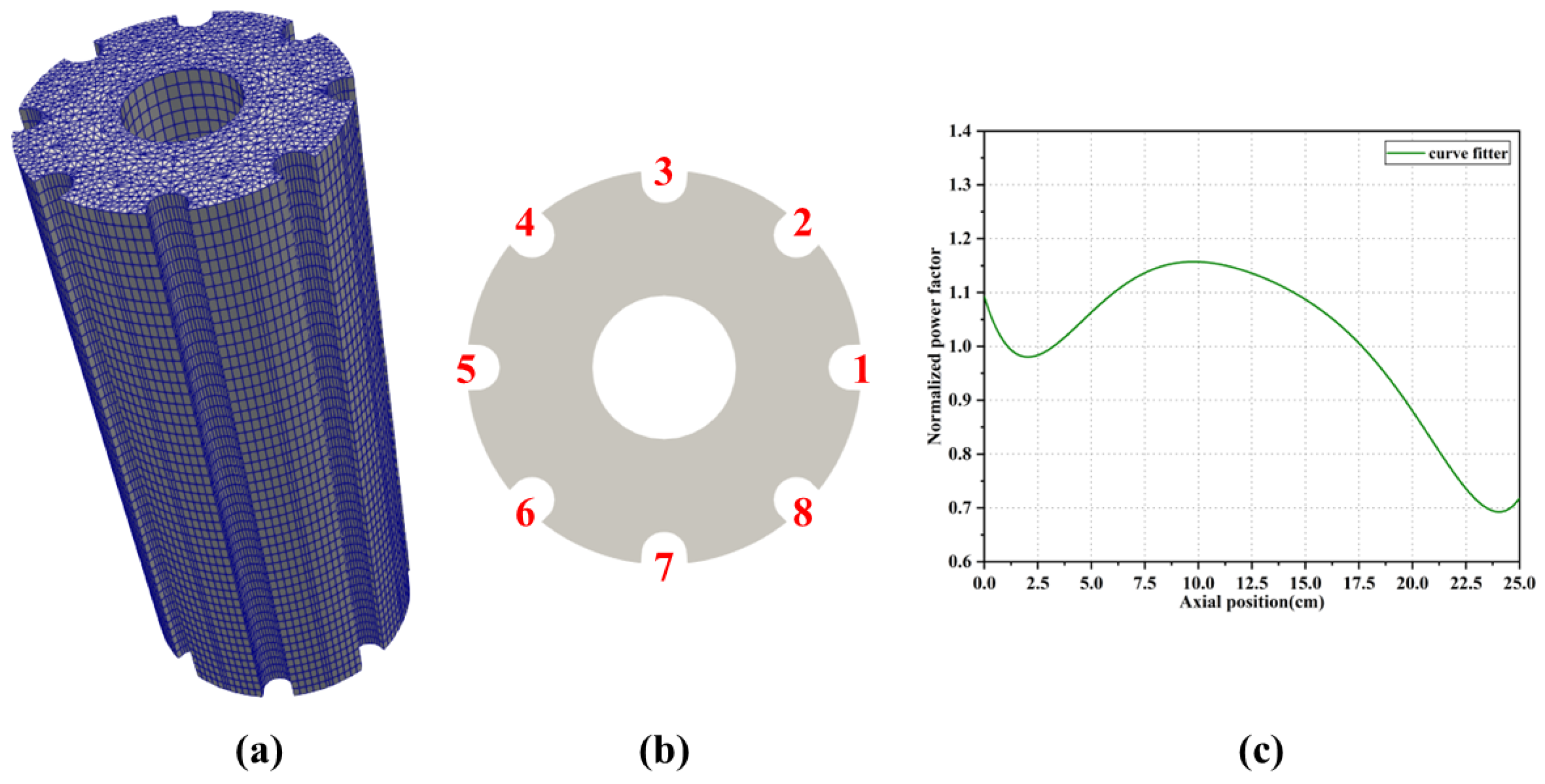
In this work, a simplified KRUSTY model is adopted for the simulations. The detailed configuration and grid of the core are presented in Figure 11a. Meanwhile, the eight heat pipes in the core are numbered, as illustrated in Figure 11b. In the core heat conduction analysis, a uniform power distribution is assumed in the radial direction. In the axial direction, the power distribution is specified according to the axial power profile that is shown in Figure 11c. The detailed parameters of the core, heat pipes, and Stirling engines are listed in

Table 2. Parameters of the core, heat pipe and Stirling engines.

Parameter	Value
Reactor outer diameter/m	0.11
Reactor height/m	0.25
Working fluid of heat pipe	Na
Length of evaporator section/m	0.25
Length of evaporator section/m	0.35
Length of evaporator section/m	0.4
Heat pipe outer diameter/m	0.0254
Heat pipe wall thickness/m	0.00178
Vapor core radius/m	0.01
Container material	Haynes-230
Wick material	Ni
Regenerator efficiency	0.8
Compression ratio	1.22
Time constant of the regenerator	80,000
Specific heat	12.5

.

3.2.1. Reactivity Insertion Transient Conditions

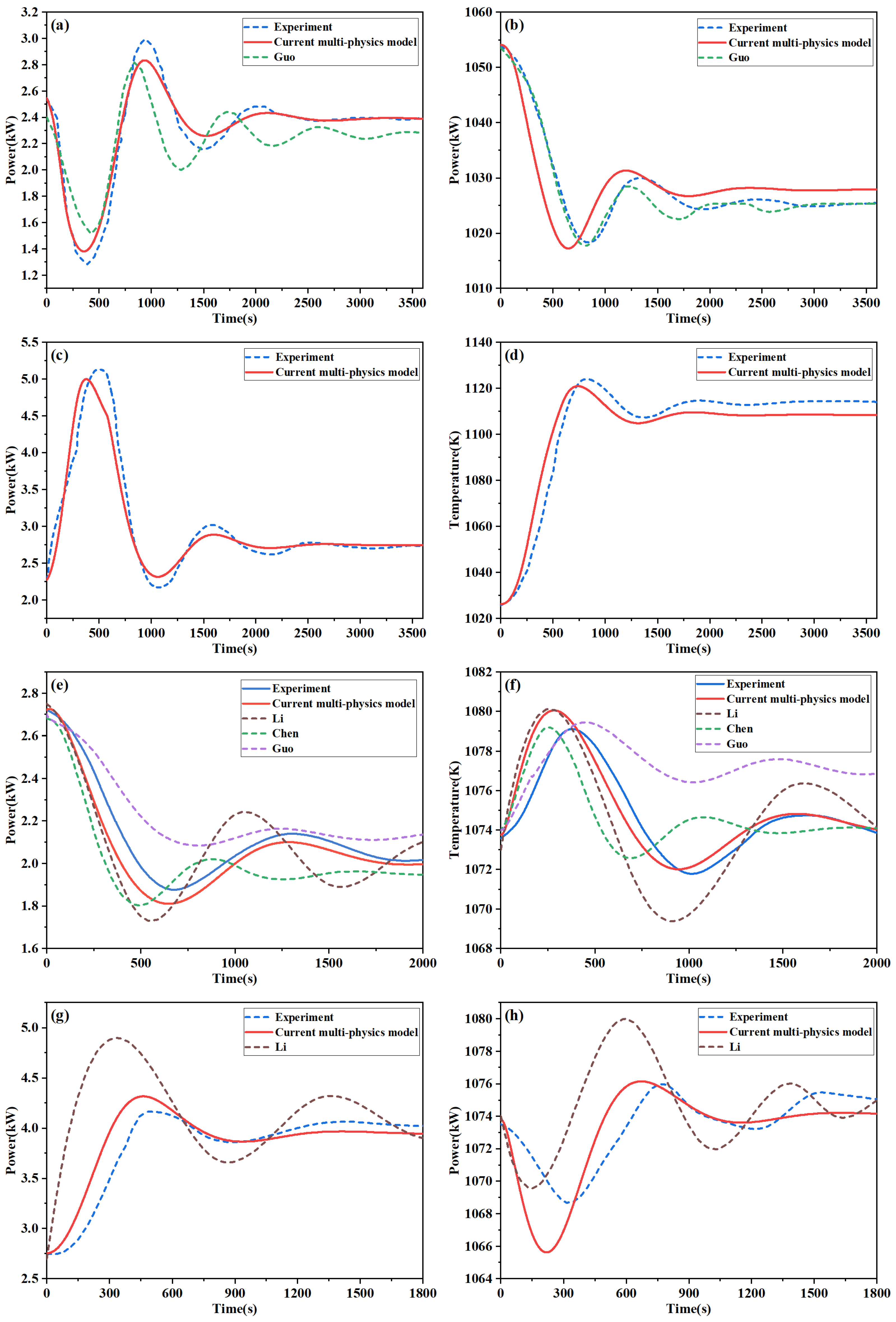
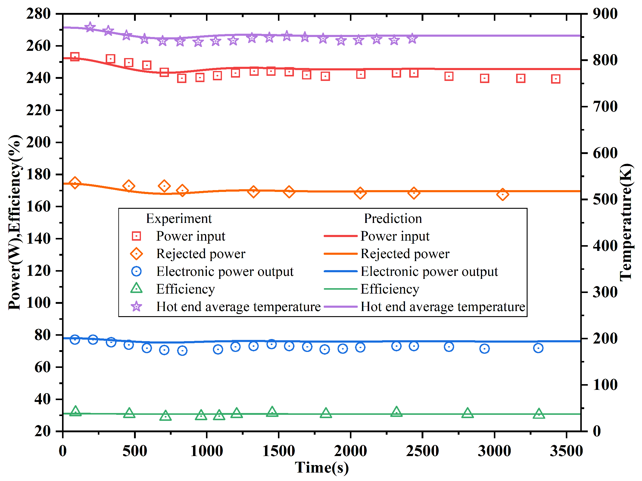
In the negative reactivity insertion experiment [32], the movable reflector is slowly lifted by 0.5 mm during the 17.00–17.05 h period, inserting 5.5 cents of negative reactivity. The comparison between the calculated and experimental results is shown in Figure 12a,b. Meanwhile, comparisons are also conducted with the validation results reported by Guo [25], and the power variations obtained in this work show closer agreement with the experimental data. Following the introduction of negative reactivity, the core power decreases rapidly, leading to a reduction in temperature. The negative temperature feedback subsequently compensates for the inserted negative reactivity within 360 s while simultaneously introducing positive reactivity. As a result, the core power and temperature gradually increase and eventually stabilize after a brief oscillation. The predicted variations in core power and average temperature show good agreement with the experimental data, with maximum relative errors of 5% and 0.6%, respectively. The simulation results indicate that the average core temperature decreased by approximately 26.2 K, which is in good agreement with the experimentally measured temperature difference of 28.6 K. However, the predicted temperature variation is observed to reach its peak more rapidly than that measured in the experiment. This discrepancy is likely attributed to the simplified reactor geometry model as well as the deviations between the thermal physical parameters of materials used in the simulation and those of the actual system. The variations in the Stirling engine parameters are shown in Figure 13, and the predicted results show good agreement with the experimental data, with the maximum relative error controlled within 8%. This demonstrates that the quasi-steady-state Stirling model employed in this work is capable of adequately describing the parameters variations in the actual Stirling engine parameters.

In the positive reactivity insertion experiment, from T = 18.00 h to T = 18.16 h, the platen is gradually raised by 1.5 mm, introducing a total of approximately 17.8 cents of positive reactivity. Figure 12c,d present the predicted variations in core power and temperature obtained from the simulation. Following the introduction of positive reactivity, the core power and average temperature increased rapidly. Owing to the negative temperature feedback effect, both power and temperature are suppressed and gradually stabilized after several oscillations. The predicted variations in core power and average temperature also show good agreement with the experimental data, with maximum relative errors of 8.3% and 1.3%, respectively. Consistent with the negative reactivity insertion case, the core average temperature in the simulation reaches its peak more rapidly than that observed in the experiment.

3.2.2. Load Following Transient Conditions

In the KRUSTY experiment, at T = 8 h, the flow rate of the gas-cooled simulator was reduced by half, resulting in an approximately 20% decrease in the power output of each Stirling engine, thereby simulating a transient process of core load reduction. As the cooling capacity of the heat pipes decreases, heat accumulation causes the temperatures of both the heat pipes and the reactor core to increase. This temperature rise induces a negative temperature feedback effect, which decreases the reactor power and suppresses further temperature increases, resulting in only minor temperature fluctuations. In this work, this transient condition is simulated by modifying the cooling temperature boundary condition at the condenser section of the heat pipes. A comparison between the simulation results and the experimental data is presented in Figure 12e,f. The simulation results indicate that the predicted variations in reactor power and average temperature are in good agreement with the experimental data. The maximum relative error of power is 4% and 0.14% for temperature. Compared with the results reported by Li [18], Chen [20], and Guo [14], the predicted power and temperature variations obtained in this work exhibit higher accuracy. This indicates that the tight coupling between core heat transfer and heat pipes can improve numerical accuracy, while the multi-node thermal resistance network model adopted for the heat pipes is able to provide more accurate boundary conditions.

At T = 10.2 h, the cooling power of the gas-cooled simulator is increased by about 73%, representing a transient condition corresponding to an increase in core load. As the cooling capacity of the heat pipes increases, the temperatures of both the heat pipes and the reactor core decrease. Due to the negative temperature feedback effect, the reactor power increases and suppresses further temperature decreases. Figure 12g,h present a comparison between the calculated results and the experimental data. The maximum relative error of power is 13.7%, while that of temperature is 0.4%.

3.3. The Safety Analysis of KRUSTY

In the safety performance analysis of HPRs, particular attention is paid to whether the temperatures of the core and structural materials exceed their safety limits under accident conditions. Typical accident scenarios include heat pipe failure and step reactivity insertion accidents. Both types of accidents can cause a rapid rise in core temperature within a short period, potentially leading to the melting of fuel and structural materials. In Section 3.2, the accuracy of the present transient coupling framework and the associated parameters is verified through numerical simulations under four experimental conditions. Therefore, in this section, several hypothetical accidents are analyzed to evaluate the safety performance of the KRUSTY. The melting points of the key structural materials used in the KRUSTY reactor are listed in

Table 3. Melting points of core fuel and structural materials.

Material	Value
U8Mo fuel (Idaho National Laboratory, Idaho Falls, ID, USA)	1400 K
Haynes-230 (Haynes International, Kokomo, IN, USA)	1574 K
Ni in heat pipe wick (Los Alamos National Laboratory, Los Alamos, NM, USA)	1728 K

.

3.3.1. Reactivity Insertion Accident

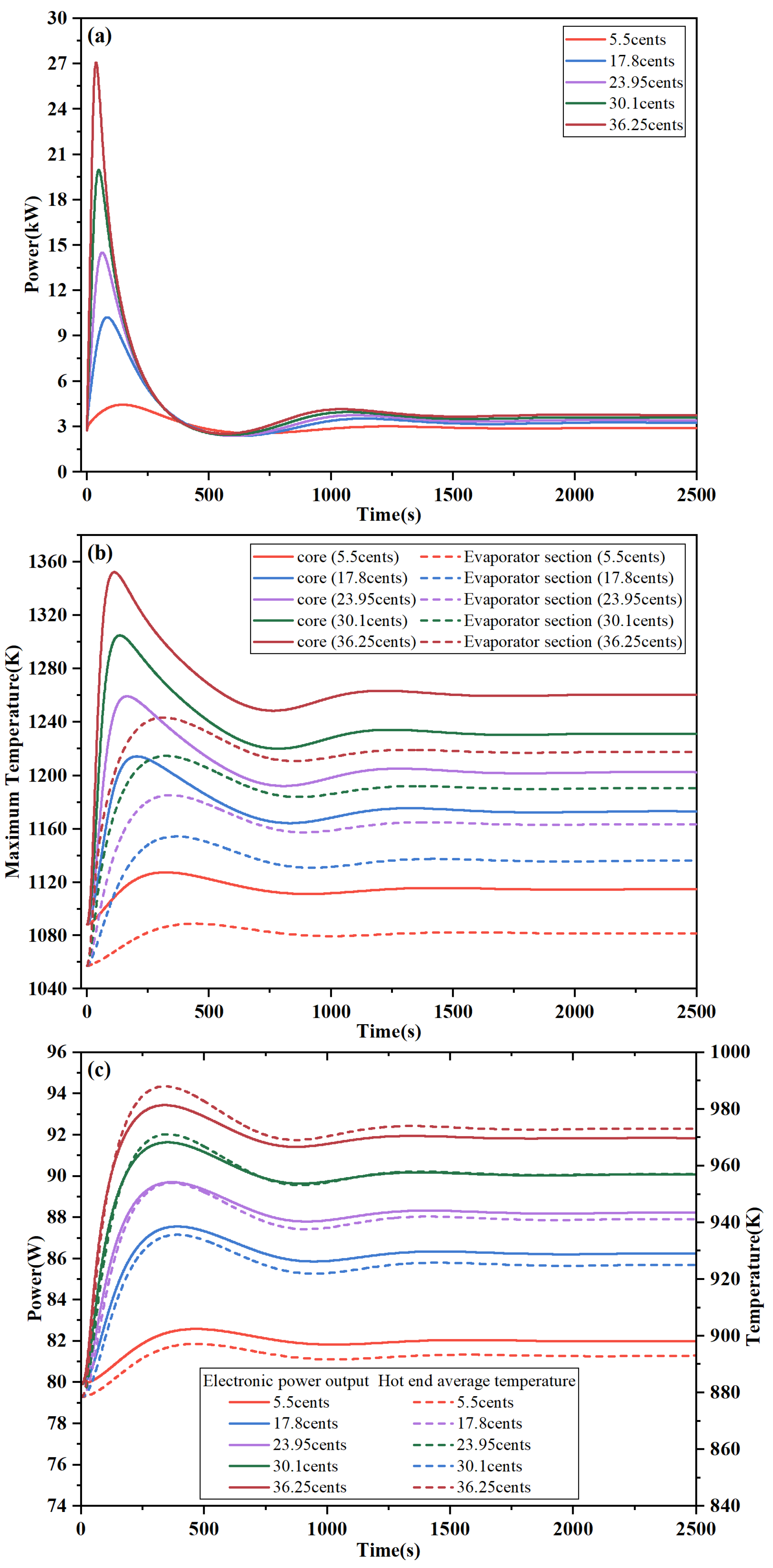
In the KRUSTY reactor, a reactivity insertion accident is typically caused by an unintended displacement of the BeO radial reflector in the reactor’s Comet platen, resulting in a sudden step reactivity insertion into the core. In this section, five hypothetical step reactivity insertion accidents are considered, with detailed accident descriptions and the corresponding power and temperature parameters listed in

Table 4. Power and temperature parameters of the core and heat pipes in the positive reactivity insertion accident.

Case	Positive Reactivity Insertion	${\mathit{P}}_{\mathit{final}}$ of Core, kW	${\mathit{P}}_{\mathit{max}}$ of Core, W	${\mathit{T}}_{\mathit{max}}$ of Core, K	${\mathit{T}}_{\mathit{max}}$ of HP, K
PRI1	5.5	2.91	4.46	1127.42	1088.91
PRI2	17.8	3.25	10.23	1214.29	1154.34
PRI3	23.95	3.42	14.51	1259.35	1185.23
PRI4	30.1	3.59	19.96	1304.96	1214.57
PRI5	36.25	3.76	27.07	1352.29	1243.33

. In all accidents, the positive reactivity is instantaneously introduced at t = 0. The variation in core power is shown in Figure 14a. The step insertion of positive reactivity causes a rapid increase in core power over a short period. Owing to the negative temperature reactivity coefficient, the power begins to decrease after reaching a peak value. In the most severe PRI5 accident, the peak core power reaches 27.07 kW, and the output power of a single heat pipe reaches 3.38 kW, which attains the capillary limit of such sodium heat pipe. The maximum temperature variations of the core and heat pipes are shown in Figure 14b. The temperature follows the variation in core power but exhibits a certain time delay. Similarly, in the PRI5 accident, the maximum core temperature reaches 1352.29 K, which is close to the melting point of the fuel. Therefore, to avoid severe safety consequences, accidental insertion of the movable reflector by more than 3.0 mm into the core should be prevented, indicating that additional design considerations are required for the KRUSTY reactor.

Figure 14c illustrates the variations in the electrical power output and the hot-end temperature of the Stirling engine. The trends of both parameters are generally consistent with the variation in the heat pipe temperature. In the PRI5 accident, the peak hot-end temperature of the Stirling engine reaches 988.05 K, and the peak electrical power output reaches 93.44 kW. Compared with the initial operating condition, these values increase by 12.5% and 16.9%, respectively. These results indicate that the impact of the positive reactivity step accident on the energy conversion system is acceptable and does not lead to excessively high power output or temperature in the Stirling engine.

3.3.2. Heat Pipe Failure

Unlike pressurized water reactors or gas-cooled reactors, HPRs rely on high-temperature alkali metal heat pipes to transfer heat from the core. Consequently, flow-loss accidents caused by mechanical failures such as pump shutdowns cannot occur in HPRs. However, during long-term operation in the reactor core, high-temperature alkali metal heat pipes may experience potential failures due to chemical oxidative corrosion or intense neutron irradiation. Such failures can severely degrade the reactor heat removal capability, leading to excessive heat accumulation within the core. Most studies on heat pipe failure accidents focus on steady-state calculations. However, this approach completely neglects the effect of the negative temperature reactivity coefficient of the core and therefore leads to a significant overestimation of accident severity. Consequently, transient analyses of heat pipe failure accidents in the KRUSTY core are performed in this work. The corresponding heat pipe failure scenarios are listed in

Table 5. Power and temperature parameters of the core and heat pipes in the heat pipe failure accident.

Case	Heat Pipe Failure	${\mathit{P}}_{\mathit{final}}$ of Core, kW	${\mathit{P}}_{\mathit{max}}$ of HP, W	${\mathit{T}}_{\mathit{max}}$ of Core, K	${\mathit{T}}_{\mathit{max}}$ of HP, K
HPF1	#1	2.55	421.23	1105.32	1066.52
HPF2	#1#3	2.33	506.50	1105.93	1076.67
HPF3	#1#2	2.32	436.67	1143.97	1059.70

.

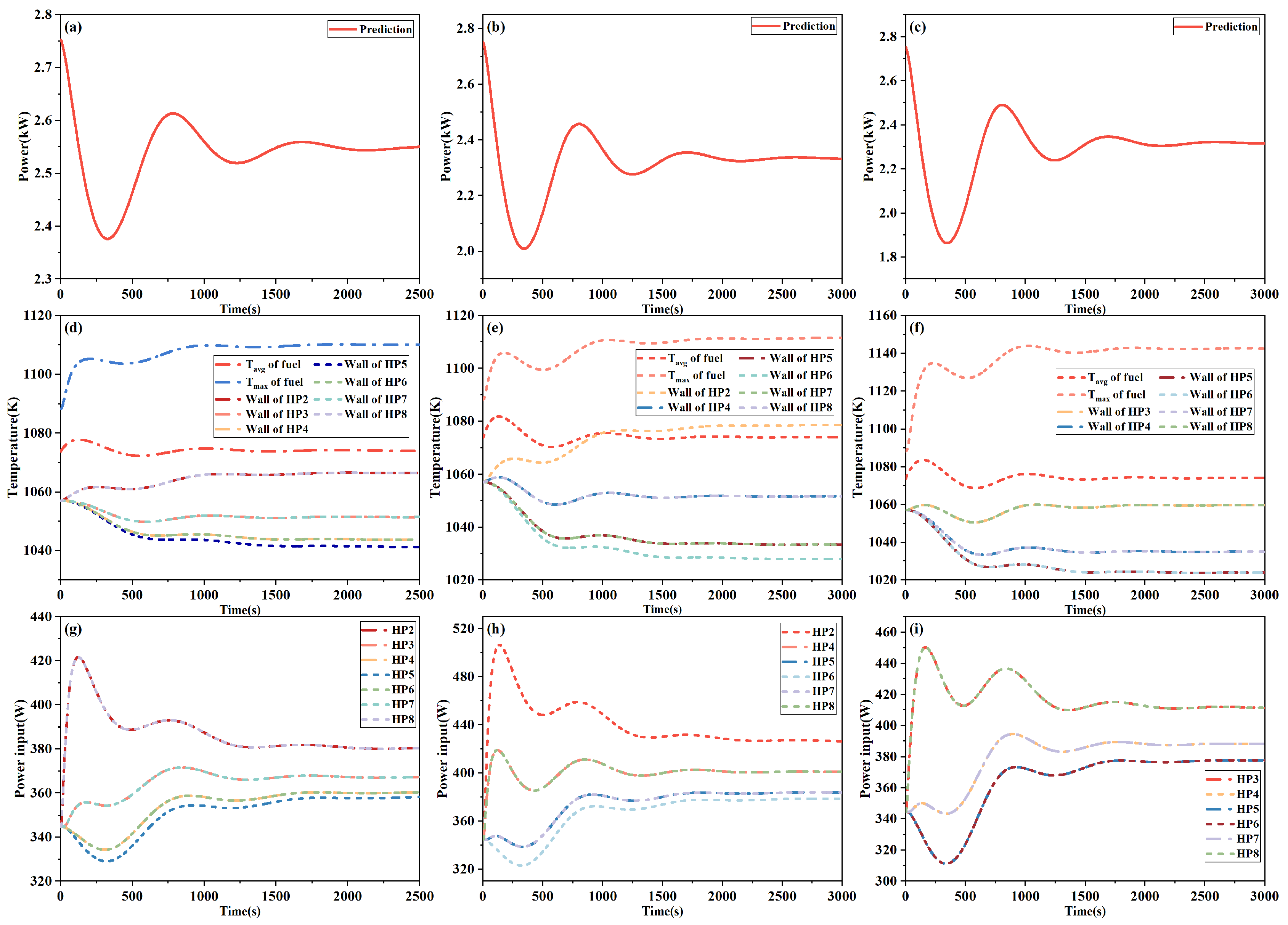
Figure 15 presents the variations in core and heat pipe power and temperature under three heat pipe failure accident scenarios. As shown in Figure 15a–c, the core power in all three cases gradually decreases due to the effect of negative temperature feedback and eventually stabilizes at 2.55, 2.33, and 2.32 kW, respectively. As illustrated in Figure 15d–f, the average core temperature initially increases and then decreases. This behavior results from short-term heat accumulation caused by heat pipe failure, followed by an overall temperature reduction as the core power decreases. In contrast, the maximum core temperature exhibits a trend of an initial increase, a subsequent decrease, and then a further increase. This is due to the severe heat accumulation occurring in the region of the failed heat pipe. Although the reduction in core power temporarily lowers the maximum temperature, the local temperature continues to rise with time. The maximum temperature of the heat pipe wall is primarily influenced by the core power, and only the heat pipes located closest to the failed one experience a noticeable temperature increase. In the HPF1 case, temperature increases are observed in HP2 and HP8, whereas in the HPF2 case, a temperature increase occurs in HP3. In the HPF3, temperature increases are observed in both HP3 and HP8. In the three heat pipe failure accidents, the peak maximum core temperatures are 1105.32 K, 1105.93 K, and 1143.97 K, respectively. These core temperatures remain well below the safety limits of the KRUSTY core, indicating that core safety can be ensured without human intervention even in the event of the simultaneous failure of two adjacent heat pipes.

The variations in the input power of heat pipe shown in Figure 15g–i further confirm this behavior. Except for the heat pipes located closest to the failed heat pipe, whose input power increases significantly over a short period, the input power of the remaining heat pipes decreases as a result of the reduction in core power. As the core power continues to decrease, the input power of the adjacent heat pipes gradually declines, and a portion of the power is instead redistributed to other heat pipes. Consequently, the input power of these heat pipes begins to increase. However, the magnitude of these increases are insufficient to induce a noticeable change in heat pipe temperature.

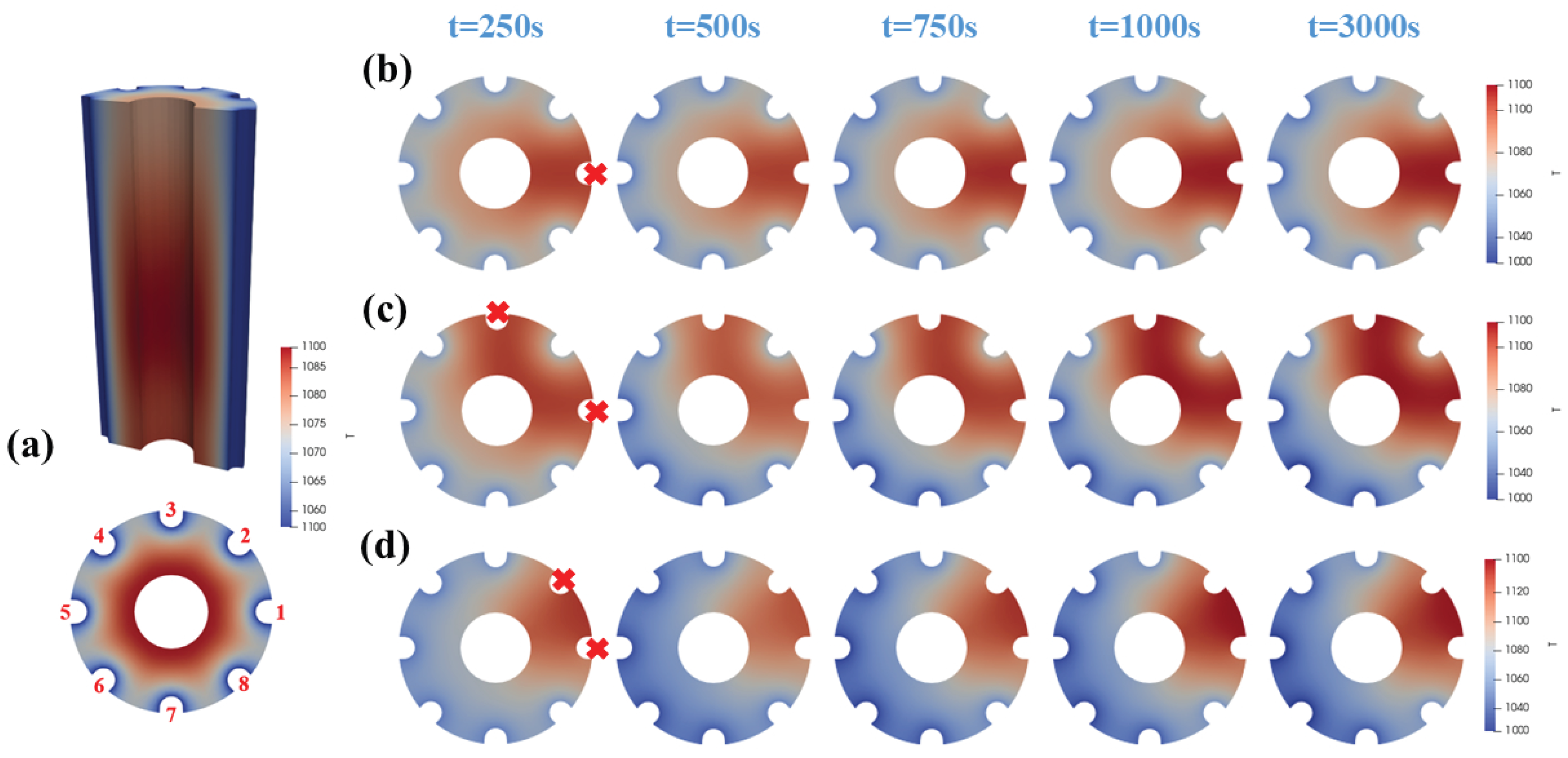
Figure 16 shows the temporal evolution of the temperature radial distribution at the center section of the core. In the HPF1, heat is mainly accumulated in the vicinity of HP1, and the affected fuel region is the smallest. In the HPF2, although HP2 continues to operate normally, heat is still primarily accumulated in the fuel region between HP1 and HP3, resulting in the largest area exhibiting a noticeable temperature increase. In the HPF3, a significant temperature rise is observed in the fuel located between HP1 and HP2, particularly near the boundary. In all heat pipe failure accidents, fuel regions located farther from the failed heat pipe exhibit smaller temperature increases, and temperature even decreases as the core power decreases.

4. Conclusions

This paper develops a transient coupled analysis framework for HPRs based on the multi-physics coupling code MOOSE. The core heat transfer module, point kinetics module, heat pipe module (including thermal resistance network and closed-form analytical model) and Stirling engine module involved in this framework are both developed within MOOSE. A new approach based on MOOSE is proposed for developing both the multi-node thermal resistance network model and the closed-form analytical solution model, enabling the two models to be simultaneously invoked within a single numerical simulation. All modules are validated through the heat pipe experiments and KRUSTY transient experiments. In addition, accident analyses are conducted on the KRUSTY reactor system to investigate core safety performance. The conclusions are as follows:

(1)

The developed framework is used to simulate the transient operating conditions of the KRUSTY reactor system and is compared with other multi-physics models. In contrast, the current multi-physics model demonstrates higher numerical accuracy. Under reactivity insertion conditions, the maximum relative error of the simulations is only 8.3%, whereas a maximum relative error of only 13.7% is observed under core load variation conditions. These are much lower than the maximum relative error of other multi-physics coupling models under the same conditions.

(2)

In the hypothetical most severe heat pipe failure accident, the predicted maximum temperature of the KRUSTY core is only 1144 K. This demonstrates that the inherent negative temperature reactivity coefficient of the core, together with the redistribution of power to the remaining operational heat pipes, can effectively mitigate heat pipe failure accidents. In contrast, other studies often evaluate heat pipe failure accidents using simplified steady-state calculations in which the negative temperature feedback of the core is neglected, leading to a significant overestimation of accident severity.

(3)

In heat pipe failure accidents, core power does not merely accumulate locally but is dynamically redistributed. Although short-term heat accumulation may occur in the vicinity of the failed heat pipe, the power is subsequently redistributed to the remaining operational heat pipes, thereby establishing a new thermal equilibrium state. During the initial period following the failure, the three relatively distant heat pipes do not assume any additional power load, indicating that further optimization of the heat pipe arrangement in KRUSTY is still possible.

However, there are some limitations and aspects for improvement in this framework. First, the point kinetics module currently employed is unable to simulate variations in the core power shape. Therefore, a neutron transport code based on the MOOSE framework is under development. Second, the Stirling model adopted in this study is steady-state only and cannot be truly coupled with the other modules. Consequently, a transient Stirling model will be addressed in future work.

References

1. Guo, Y.-C.; Su, Z.-L.; Li, Z.-G.; Wang, K. Numerical investigation on the startup performance of high-temperature heat pipes for heat pipe cooled reactor application. Nucl. Sci. Tech. 2021, 32, 104. [Google Scholar] [CrossRef]
2. Fan, Y.; Yan, R.; Zhu, G.; Chen, L.; Zhang, N.; Zou, Y. Design of a prismatic CERMET megawatt gas-cooled reactor(PC-MGCR) for deep space exploration. Ann. Nucl. Energy 2025, 211, 110946. [Google Scholar] [CrossRef]
3. Cheng, H.; Cheng, S.; Chen, S. Sodium fast reactors. In Nuclear Power Reactor Designs; Elsevier: Amsterdam, The Netherlands, 2024; pp. 185–208. [Google Scholar] [CrossRef]
4. Ashraf, O.; Rykhlevskii, A.; Tikhomirov, G.V.; Huff, K.D. Preliminary design of control rods in the single-fluid double-zone thorium molten salt reactor (SD-TMSR). Ann. Nucl. Energy 2021, 152, 108035. [Google Scholar] [CrossRef]
5. Cui, D.Y. Preconceptual nuclear design of a 50 kWth heat pipe cooled micro molten salt reactor (micro-MSR). Prog. Nucl. Energy 2021, 134, 103670. [Google Scholar] [CrossRef]
6. Poston, D.I.; Kapernick, R.J.; Guffee, R.M. Design and analysis of the SAFE-400 space fission reactor. AIP Conf. Proc. 2002, 608, 578–588. [Google Scholar] [CrossRef]
7. Gibson, M.A.; Oleson, S.R.; Poston, D.I.; McClure, P. NASA’s Kilopower reactor development and the path to higher power missions. In Proceedings of the 2017 IEEE Aerospace Conference, Big Sky, MT, USA, 4–11 March 2017; pp. 1–14. [Google Scholar] [CrossRef]
8. Poston, D.I. The Heat Pipe-Operated Mars Exploration Reactor (HOMER). AIP Conf. Proc. 2001, 552, 797–804. [Google Scholar] [CrossRef]
9. El-Genk, M.S. Conceptual Design of HP-STMCs Space Reactor Power System for 110 kWe. AIP Conf. Proc. 2004, 699, 658–672. [Google Scholar] [CrossRef]
10. El-Genk, M.S.; Tournier, J.-M.P. “SAIRS”—Scalable Amtec Integrated Reactor Space Power System. Prog. Nucl. Energy 2004, 45, 25–69. [Google Scholar] [CrossRef]
11. McClure, P.R.; Poston, D.I.; Gibson, M.A.; Mason, L.S.; Robinson, R.C. Kilopower Project: The KRUSTY Fission Power Experiment and Potential Missions. Nucl. Technol. 2020, 206, 2. [Google Scholar] [CrossRef]
12. Wu, A.; Wang, W.; Zhang, K.; Shen, S.; Duan, W.; Pan, R.; Luo, X.; Chen, H. Multiphysics Coupling Analysis of Heat Pipe Reactor Based on OpenMC and COMSOL Multiphysics. Ann. Nucl. Energy 2023, 194, 110115. [Google Scholar] [CrossRef]
13. Wang, W.; Zhang, K.; Dong, S.; Wang, S.; Chen, H. Analysis of heat pipe cooled reactor startup characteristics by multi-physics coupling simulation based on MOOSE framework. Nucl. Eng. Des. 2025, 441, 114164. [Google Scholar] [CrossRef]
14. Guo, Y.; Li, Z.; Wang, K.; Su, Z. A transient multiphysics coupling method based on OpenFOAM for heat pipe cooled reactors. Sci. China Technol. Sci. 2022, 65, 102–114. [Google Scholar] [CrossRef]
15. Zhang, D.; Zhang, N.; Li, Z.; Ren, Y.; Su, Z.; Yu, G.; Zhong, G.; Ding, H. Multiphysics Coupling Analysis of Heat Pipe Reactor Considering Irradiation Effects Based on RMC and FEniCSx. Nucl. Eng. Des. 2025, 444, 114414. [Google Scholar] [CrossRef]
16. Jeong, M.J.; Im, J.; Lee, S.; Cho, H.K. Multiphysics Analysis of Heat Pipe Cooled Microreactor Core with Adjusted Heat Sink Temperature for Thermal Stress Reduction Using OpenFOAM Coupled with Neutronics and Heat Pipe Code. Front. Energy Res. 2023, 11, 1213000. [Google Scholar] [CrossRef]
17. Chen, J.; Zhao, R.; Lv, Z.; Xie, J.; Ni, W. Multi-Physics Coupling Computational Analysis of a Heat-Pipe-Cooled Space Molten Salt Reactor. Ann. Nucl. Energy 2026, 227, 111994. [Google Scholar] [CrossRef]
18. Li, G.; Li, H.; Tian, X.; Ouyang, Z.; Kang, X.; Li, D.; Shan, J.; Jiang, X. Improvement and Validation of the System Analysis Model and Code for Heat-Pipe-Cooled Microreactor. Energies 2022, 15, 2586. [Google Scholar] [CrossRef]
19. Feng, M.; Ouyang, Z.; Wu, P.; Shan, J. Development and Validation of Transient Analysis Code for Heat Pipe Reactor System. Ann. Nucl. Energy 2026, 226, 111817. [Google Scholar] [CrossRef]
20. Chen, H.; Wang, W.; Wu, A.; Zhang, K.; Pan, R.; Duan, W.; Yang, G.; Qin, C.; Luo, X. Multi-physics coupling analysis of test heat pipe reactor KRUSTY based on MOOSE framework. Nucl. Eng. Des. 2023, 414, 112597. [Google Scholar] [CrossRef]
21. Permann, C.J.; Gaston, D.R.; Andrš, D.; Carlsen, R.W.; Kong, F.; Lindsay, A.D.; Miller, J.M.; Peterson, J.W.; Slaughter, A.E.; Stogner, R.H.; et al. MOOSE: Enabling massively parallel multiphysics simulation. SoftwareX 2020, 11, 100430. [Google Scholar] [CrossRef]
22. Li, H.; Tian, X.; Ge, L.; Kang, X.; Zhu, L.; Chen, S.; Chen, L.; Jiang, X.; Shan, J. Development of a Performance Analysis Model for Free-Piston Stirling Power Convertor in Space Nuclear Reactor Power Systems. Energies 2022, 15, 915. [Google Scholar] [CrossRef]
23. McClure, P.R.; Poston, D.I.; Clement, S.D.; Restrepo, L.; Miller, R.; Negrete, M. KRUSTY Experiment: Reactivity Insertion Accident Analysis. Nucl. Technol. 2020, 206, 5. [Google Scholar] [CrossRef]
24. Guo, Y.; Su, Z.; Li, Z.; Wang, K.; Liu, X. An Improved Model of the Heat Pipe Based on the Network Method Applied on a Heat Pipe Cooled Reactor. Front. Energy Res. 2022, 10, 848799. [Google Scholar] [CrossRef]
25. Guo, Z.; Liu, L.; Liu, Z.; Gu, H. Development and application of a transient analysis code for heat pipe cooled reactor systems. Nucl. Eng. Des. 2024, 419, 112979. [Google Scholar] [CrossRef]
26. Cao, Y.; Faghri, A. Closed-Form Analytical Solutions of High-Temperature Heat Pipe Startup and Frozen Startup Limitation. J. Heat Transf. 1992, 114, 1028–1035. [Google Scholar] [CrossRef]
27. Li, Y.; He, Y.; Wang, W. Optimization of Solar-Powered Stirling Heat Engine with Finite-Time Thermodynamics. Renew. Energy 2011, 36, 421–427. [Google Scholar] [CrossRef]
28. Cherezov, A.; Park, J.; Kim, H.; Choe, J.; Lee, D. A Multi-Physics Adaptive Time Step Coupling Algorithm for Light-Water Reactor Core Transient and Accident Simulation. Energies 2020, 13, 6374. [Google Scholar] [CrossRef]
29. Faghri, A.; Buchko, M.; Cao, Y. A Study of High-Temperature Heat Pipes With Multiple Heat Sources and Sinks: Part I—Experimental Methodology and Frozen Startup Profiles. J. Heat Transf. 1991, 113, 1003–1009. [Google Scholar] [CrossRef]
30. Ponnappan, R. Studies on the Startup Transients and Performance of a Gas Loaded Sodium Heat Pipe. Ph.D. Thesis, Dayton University, Dayton, OH, USA, 1988. [Google Scholar]
31. Cao, Y.; Faghri, A. Transient Two-Dimensional Compressible Analysis for High-Temperature Heat Pipes with Pulsed Heat Input. Numer. Heat Transf. Part A Appl. 1991, 18, 483–502. [Google Scholar] [CrossRef]
32. Poston, D.I.; Gibson, M.A.; Sanchez, R.G.; McClure, P.R. Results of the KRUSTY Nuclear System Test. Nucl. Technol. 2020, 206, 9. [Google Scholar] [CrossRef]
Figure 1. The structure of KRUSTY [23].
Energies 19 01815 g001
Figure 2. Schematic of heat pipe heat transfer and the thermal network model.
Energies 19 01815 g002
Figure 3. The thermal network model calculation flowchart.
Energies 19 01815 g003
Figure 4. Schematic of heat pipe heat transfer in frozen startup.
Energies 19 01815 g004
Figure 5. Program structure for simultaneous invocation of heat pipe models.
Energies 19 01815 g005
Figure 6. Simplified model of the Stirling cycle.
Energies 19 01815 g006
Figure 7. Stirling cycle T-S diagram.
Energies 19 01815 g007
Figure 8. Transient calculation flowchart.
Energies 19 01815 g008
Figure 9. Picard iteration with sub-cycling in MOOSE.
Energies 19 01815 g009
Figure 10. Comparison with sodium heat pipe experiment: (a) Fagrhi, (b) Ponnappan and (c) Zuo.
Energies 19 01815 g010
Figure 11. The simplified model of KRUSTY. (a) The grid of the core. (b) The numbers of the heat pipe. (c) The axial power distribution of the core.
Energies 19 01815 g011
Figure 12. Validation results for different operating conditions. (a,b) Power and average temperature variations in negative reactivity insertion condition [25]. (c,d) Power and average temperature variations in positive reactivity insertion condition. (e,f) Power and average temperature variations in load reduction condition [14,18,20]. (g,h) Power and average temperature variations in load increase condition [18].
Energies 19 01815 g012
Figure 13. Validation with the Stirling model.
Energies 19 01815 g013
Figure 14. The variations in the core system in different reactivity insertion accidents. (a) The power of the core. (b) The maximum temperature of core and the evaporator section of heat pipe wall. (c) The Stirling engine performance.
Energies 19 01815 g014
Figure 15. The variations in the core system in different heat pipe failure accidents. (ac) The power of the core in HPF1, HPF2 and HPF3. (df) The temperature of the core and heat pipe in HPF1, HPF2 and HPF3. (gi) The power input of the heat pipe in HPF1, HPF2 and HPF3.
Energies 19 01815 g015
Figure 16. The temperature distribution of the core. (a) Axial and radial temperature distributions of the core in steady state and heat pipe numbers. (bd) Radial temperature distribution at the axial center position of the core in HPF1, HPF2 and HPF3.
Energies 19 01815 g016