Article

Non-Linear Method of Vehicle Pre-Crash Velocity Estimation Based on Random Forest Regression and Energy Equivalent Speed for Compact Vehicle Class


1
Department of Road and Urban Transport, University of Žilina, 010-26 Žilina, Slovakia
2
Institute of Information Technology, Lodz University of Technology, 93-590 Łódź, Poland
3
Institute of Theoretical and Applied Informatics, Polish Academy of Sciences, 00-901 Gliwice, Poland
4
Division of Ecotechnics, Lodz University of Technology, 90-924 Łódź, Poland
5
Faculty of Mechatronics and Mechanical Engineering, Kielce University of Technology, 25-314 Kielce, Poland
6
Faculty of Humanities, Jan Kochanowski University in Kielce, 25-369 Kielce, Poland
*
Authors to whom correspondence should be addressed.
Energies 2026, 19(7), 1678; https://doi.org/10.3390/en19071678
Submission received: 29 January 2026 / Revised: 6 March 2026 / Accepted: 26 March 2026 / Published: 29 March 2026

Abstract

Until now, there have been no published attempts to utilize ensemble learning approaches to pre-crash velocity estimation. In this research article, we focus on the method of vehicle crash velocity prediction based on the random forest regression approach. In particular, the study aims to develop and validate a random forest-based non-linear model for estimating pre-crash velocity using EES-related parameters for compact vehicles in a crash scenario against an immovable, stationary barrier. The estimation technique is trained and evaluated using the compact vehicle class from the NHTSA database, which consists of 399 records of frontal impacts against a rigid barrier. The relative error obtained for the presented calculation method is 7.57 % , with absolute error being equal to 1.12   m / s . We subsequently compare our results with some other techniques which were tested on this dataset. Despite the simplicity of random forest regression, we obtain surprisingly good results, as the method outperforms linear regressor and artificial neural network predictors, which have relative errors of 8.17 % and 9.63 % , respectively. The independence of Event Data Recorders along with the ease of obtaining the necessary data makes the proposed approach a highly desirable tool in forensic analysis, especially in cases involving older vehicles.

1. Introduction

These days, designing vehicle structures that can withstand damage in collisions requires advanced materials that do two things: they make the vehicle lighter and more comfortable by reducing noise, vibration, and harshness (NVH) [1]. Choosing modern plastics and polymer composites is an important part of this process [2]. When used in muffler housings and body panels, these materials are excellent at reducing structural sound and changing how they absorb energy in car accidents. The choice of materials has a fundamental impact on vehicle speed, in terms of mass, aerodynamics, and mechanical performance. Modern plastics and composites allow for the formation of more rounded, complex shapes that would be impossible to achieve with sheet metal stamping. New, lighter muffler designs improve mass distribution [3], which affects vehicle speed, whereas the estimation of pre-crash velocity is a vital component of road safety research, traffic management, and forensic accident reconstruction. Vehicle speed before the driver initiates a reaction directly influences the pre-crash velocity. This, in turn, has a heavy impact on the severity of crashes, for both the car and passengers inside.
Traditionally, determining vehicle speed in crash scenarios has relied on forensic accident reconstruction techniques, the accuracy of which is dependent upon available physical evidence. This particularly includes clear pre-impact tire marks (or other marks physically present on the road surface [1,2,3]), as well as the deformation of the vehicle after the impact. The latter is particularly convenient to use in conventional reconstruction methods, which quantify pre-crash velocity using parameters such as Energy Equivalent Speed (EES)—the velocity corresponding to the kinetic energy converted into plastic deformation during the impact. Several established models address the non-linearity of this problem effectively [4,5,6,7,8]. These include approaches based on neural networks (see [9]) and Gaussian process regression (see [10,11]), as well as B-splines [12,13].
For a crash of a pair of vehicles, the widely used CRASH3 algorithm [14] is employed to establish their velocities. However, if pre-impact braking occurs without leaving clear marks, reconstruction results may underestimate the true travel speed [15]. Conducting collision analysis with models such as CRASH3 often demands expert knowledge to adjust conditions to the experimental design and to interpret the obtained results. Moreover, the CRASH3 algorithm itself is essentially an extension of energy loss calculations, simplifying physics to assume collisions are inelastic.
The accuracy and accessibility of pre-crash speed estimation have been significantly enhanced by recent technological advances. Event Data Recorders (EDRs) [15,16], now widely integrated into light vehicles, provide a new source of highly accurate pre-crash data—including velocity. In general, EDRs record pre-crash information, including vehicle speed, from various sensors, typically capturing 11 samples over a 5 s pre-crash period. For vehicles in the Volkswagen Audi Group (VAG) sold in Europe, the EDR records the data element “Speed, Vehicle Indicated”, which is derived from the instrument panel and relates to the average speed measured at the front wheels, exhibiting a stable offset (e.g., 5% above true speed) when wheel slip is absent [16]. While the EDRs allow us to establish pre-crash speed in the majority of modern cars, there are still a significant number of vehicles which do not include EDRs and thus, in the case of an accident, rely on investigators to estimate pre-crash speed using other available information.
From the perspective of energy engineering and transport energy analysis, vehicle crashes represent an extreme but highly informative case of rapid energy dissipation in mechanical systems. The pre-crash kinetic energy of a vehicle is redistributed into plastic deformation work, heat generation, acoustic emissions, and residual translational and rotational motion. Among these components, the energy absorbed by structural deformation is of particular importance, as it directly reflects both vehicle design characteristics and impact severity.
Consequently, parameters such as Equivalent Energy Speed (EES) constitute a physically grounded bridge between accident reconstruction, vehicle safety engineering, and applied energy analysis. Accurate estimation of pre-crash velocity based on deformation-related energy metrics is therefore not only relevant for forensic purposes but also contributes to broader research on energy absorption efficiency, crashworthiness optimization, and sustainable vehicle structure design.

Novel Methods of Accident Reconstruction

To overcome the inherent limitations and required complexity of traditional or physical modeling methods—such as the high technical and computational requirements of finite element method (FEM) simulations or the inaccuracies of fast momentum-based methods [17]—advanced computational and data-driven approaches are utilized in an increasingly common manner. These methods include:
  • Non-Linear Energetic Methods: These techniques utilize non-linear functions based on the average deformation coefficient (Cs) and mass (often accompanied with deformation zone width Lt) to calculate deformation work and, consequently, pre-crash speed. For example, the application of tensor B-spline products with probabilistic weights offers significant accuracy enhancement, reducing pre-crash velocity determination error to as low as 5.2–8% [12,13,18], yielding a substantial improvement over linear approaches.
  • Machine Learning (ML) Approaches: Sophisticated algorithms are employed to estimate pre-crash speed or ΔV [9,10,11,19]. Artificial neural networks (ANNs), specifically a multilayer perceptron (MLP), have been applied to frontal crash data (based on mass and deformation coefficient Cs) to estimate EES, demonstrating improvements over linear approaches, achieving a mean relative error of approximately 9%. Genetic Algorithm Model Adjustment (GAMA) [8] was also successfully utilized to optimize models defining the relationship between pre-crash velocity, mass, and deformation characteristics, yielding average relative errors around 8%.
  • Image-Based Deep Learning (DL): For estimating crash characteristics directly from post-collision images, Deep Convolutional Neural Networks (CNNs) are utilized in some papers. These models learn deformation patterns to predict metrics such as ΔV (see [20]) and classify the Location of Collision (LOC), a method which offers a promising approach without requiring expensive forensic reconstruction. Video-based approaches for speed measurement utilizing deep learning also started to emerge recently [21], combining YOLO for real-time detection with Long Short-Term Memory (LSTM) networks. Their practical usefulness in crash reconstruction remains to be seen, as video material from an appropriate perspective is infrequently available.
  • Simulation-Based Modeling: To efficiently compute collision severity parameters, time-discrete simulation tools (like impactEES [17]) use 2D vehicle substitute models derived from 3D EES models and fundamentals of mechanical impact calculation, enabling rapid calculation along with comparison against real crash-test data.
  • Vision-Based Monocular Methods: Monocular camera systems, a cost-efficient alternative to range sensors, traditionally use homographies to map the road plane to a Bird’s Eye View (BEV) or rely on measuring displacement between virtual intrusion lines [22]. However, these methods can suffer from the Projection Displacement Difference (PDD) problem, where above-plane features (like license plates) are incorrectly mapped to the ground plane, leading to speed overestimation. A motion plane-based approach proposed in [23] addresses this by using the license plate center as a reference point and estimating the hypothetical plane on which it moves via a Shape-from-Template (SfT) technique, thereby mitigating PDD and significantly reducing the need for camera calibration. These techniques have not been widely utilized in accident analysis yet. Nevertheless, with growing access to data collected just prior to the accident, said methods also indicate an interesting direction of research.
  • For risk injury assessment, it has been proven that impact-related variables are of greater significance than the vehicle-related features [24]. The results obtained by the authors in both [24,25] indicate that pre-crash speed estimation techniques are not the only possible way to utilize the impact data—this information can also be utilized to reduce the risks related to vehicle operation in general.
This diversity of techniques highlights the ongoing efforts to achieve robust and highly accurate velocity estimation across various application domains and utilization of a broad range of accessible information.
As far as the ensemble methods considered in the scope of crash reconstruction, accident prevention and monitoring, and similar topics are concerned, they have a large range of applications. Listing all papers which utilize ensemble methods in forensics would be nearly impossible—below, we list a short selection of the more recent articles we have found quite interesting:
  • In ref. [26], the authors utilize driver input data (such as braking, steering wheel usage, etc.) for predicting a binary variable indicating whether the driver participated in an accident.
  • The authors of [27,28] use ensemble methods (the first one uses simpler techniques, and the latter uses a rather sophisticated attention-based transformer accompanied with a conformer) to predict the likelihood of a crash based on the infrastructure-based detector data. The initial limitations of the low coverage from such data are alleviated via the connected vehicle trajectory data discussed in [28].
  • Lastly, the neat article by Wu, Meng and Song [29] provides a nice exposition of prediction of the number of crashes in various regions of China utilizing (among others) ensemble methods for CART trees for prediction and selection of the most influential variables.
The authors have failed to spot any previously documented results in the prediction of pre-crash velocity in particular—this paper directly addresses this research gap.
In this paper, we investigate the application of various approaches based on random forests to see whether we are able to provide a viable method for pre-crash velocity estimation for the purpose of accident reconstruction. In Section 2, we describe the dataset and discuss some advantages and disadvantages of random forest applications in regression tasks. The Section 3 is devoted to presenting obtained results along with an in-depth analysis of the obtained method. A subsequent comparison of the effectiveness of random forest against classic linear regressors follows. The Section 4 is devoted to discussion of the potential use of RF in comparison to other techniques viable for the compact vehicle class as well as further research directions.
From an energy-oriented standpoint, the majority of modern accident reconstruction techniques can be interpreted as indirect methods for estimating the portion of kinetic energy dissipated during impact. Machine learning-based approaches, in particular, provide a flexible framework for modeling highly non-linear energy transfer mechanisms without explicitly formulating complex constitutive or contact models.
In this context, ensemble learning methods such as random forests offer a practical compromise between physical interpretability and predictive accuracy. By learning from empirical relationships between deformation-related variables and pre-crash velocity, these models implicitly capture energy absorption patterns characteristic of a given vehicle class, impact configuration, and structural design philosophy.
In view of the above, this study contributes to the field of crash reconstruction by developing a random forest model for estimating pre-crash velocity in compact passenger cars involved in full-width frontal impacts against a rigid barrier. The proposed approach is validated using NHTSA crash-test data with a stratified train–test split and 5-fold cross-validation. In addition, the performance of the developed model is compared with selected alternative methods, including linear regression, a single-layer neural network, and gradient-boosted tree ensembles. To improve the transparency of the proposed solution, model behavior is further analyzed using SHAP values and permutation feature importance. This study also provides a reproducible analytical workflow based on a clearly defined preprocessing, training, and evaluation procedure.

2. Materials and Methods

From the perspective of applied energy analysis, the adopted methodology focuses on reconstructing the pre-impact kinetic energy state of the vehicle using post-impact deformation measurements. The random forest regression model does not explicitly calculate deformation work; instead, it learns the functional relationship between measurable deformation-related indicators and the velocity-equivalent energy state represented by EES. This data-driven formulation allows the model to account for complex energy dissipation mechanisms that arise from structural heterogeneity, localized stiffness variations, and non-linear material behavior, which are difficult to represent using simplified analytical or momentum-based approaches.
Before proceeding with the general method description, we start by shortly discussing the most important features of the considered dataset.

2.1. Dataset Description

The collected data describes crashes at speeds between 4.5 and 27   m / s . Of the observations, 78% revolve around velocities ranging from 13 to 16   m / s . The full dataset ( n   =   399 ) was partitioned into training and evaluation subsets. Specifically, 10 % of the data was reserved for testing, while the remaining 90 % was used for model training and selection by means of cross-validation, as discussed in subsequent paragraphs.
Because the target variable is continuous, stratified sampling was implemented by first discretizing the target values into five equally spaced bins and then performing a stratified random split based on these bins. This ensured that the empirical distribution of the target variable was preserved across the training and evaluation subsets.
The data partitioning was performed using a fixed random seed 123 to guarantee reproducibility. Model hyperparameters were optimized using 5-fold cross-validation on the training subset only, while the held-out evaluation subset was used exclusively for performance assessment. The loss function utilized in training is squared error, which is a standard approach in a multitude of regression problems.
A brief description of the dataset along with some basic characteristics is included in subsequent Table 1. It contains information on deformation coefficients C i   [ m ] along with the average deformation C s   [ m ] , impact zone width (deformation width) L t   [ m ] , vehicle mass m a s s   [ k g ] , and observed pre-crash speed V t   [ m s ] .
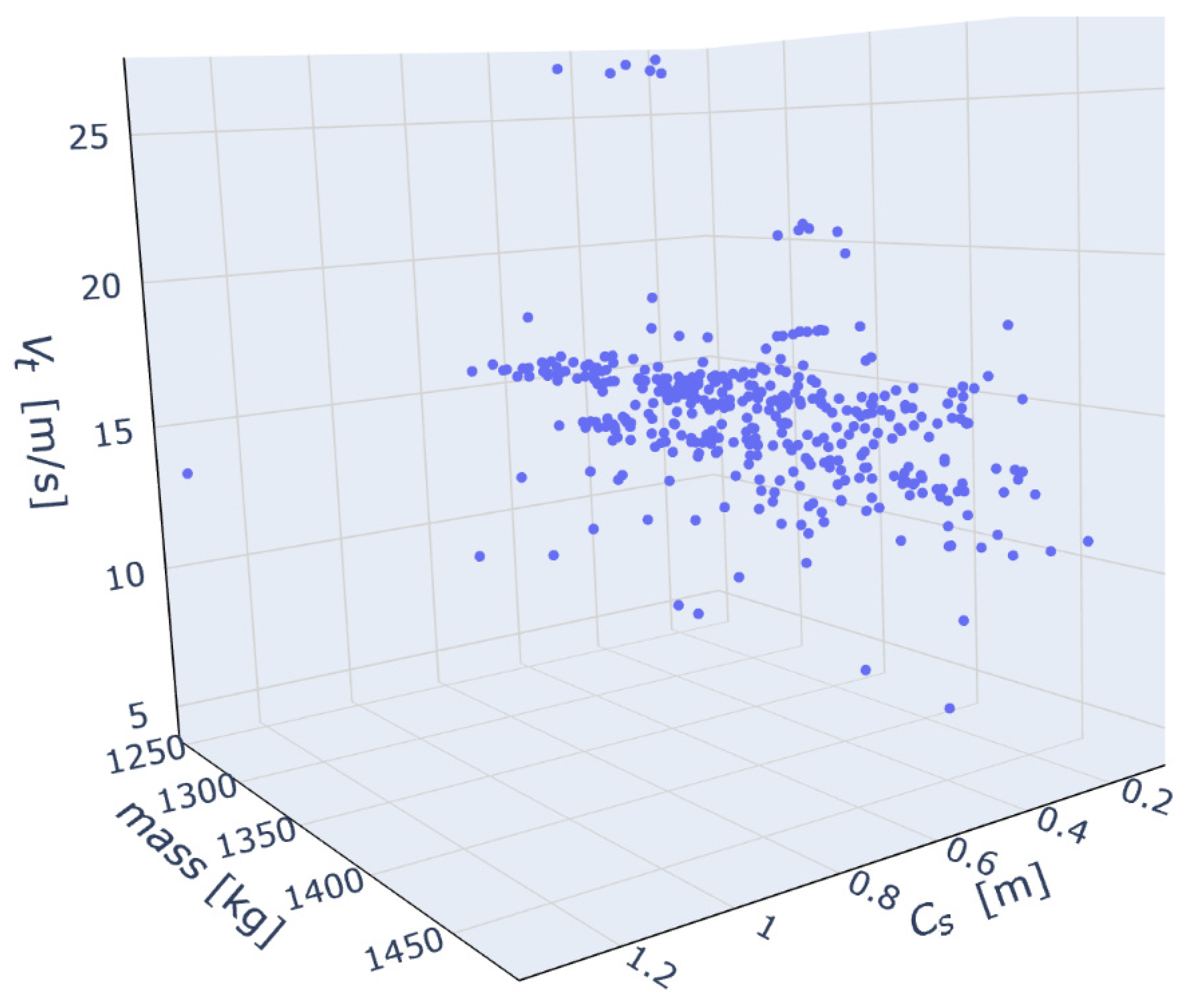
The structure of the dataset indicates quite uneven distribution, which can be (at least partially) seen in Figure 1. We can notice some deviating observations outside of the general surface, which is heavily determined by the central half of the data.
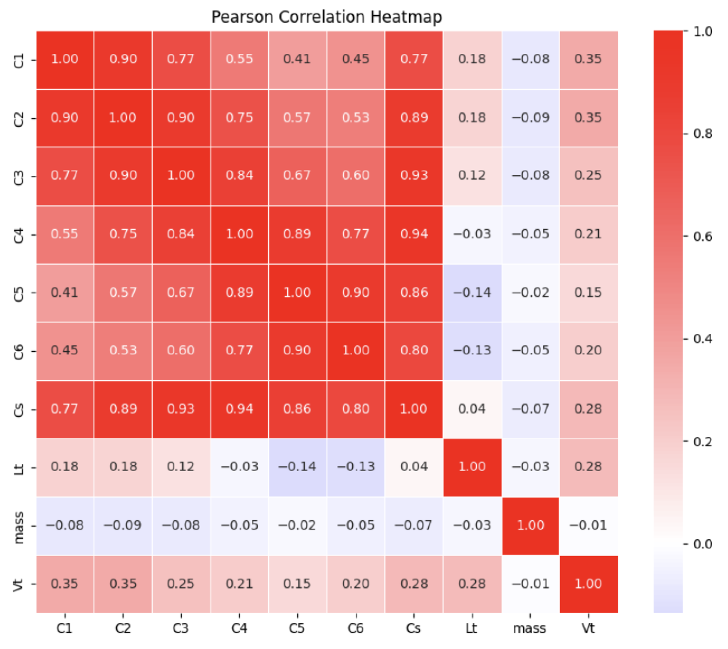
The scatterplot is one thing; the correlation heatmap (Figure 2) below displays the connection between particular variables. The most interesting from our perspective is the relationship between the pre-crash velocity V t and the remaining variables.
Unsurprisingly, the variables which are strongly correlated with V t are the impact-related ones, while mass seems to be mostly independent from V t . This phenomenon is quite easily explained by a moderate variance of the m a s s parameter and the relationship between the vehicle mass and deformation from the impact. These observations remain consistent with the observations contained in [24,25].
The strong connection between variables C i i = 1 , , 6   and the average deformation C s is rather obvious due to the way the deformation coefficient C s is calculated. While details on the measurements can be found in [30], for the sake of this paper’s completeness, we provide brief information on the topic in Section 2.2.

2.2. Measuring the Average Deformation Coefficient C s

Utilizing the principle of a simple moving average of order 5 and then taking the mean value of the results, we arrive at the following formula for C s , which is widely established in the literature (see [9,30,31] as well as references therein) (1):
C s C 2 + C 3 + C 4 + C 5 5 + C 1 + C 6 10 .
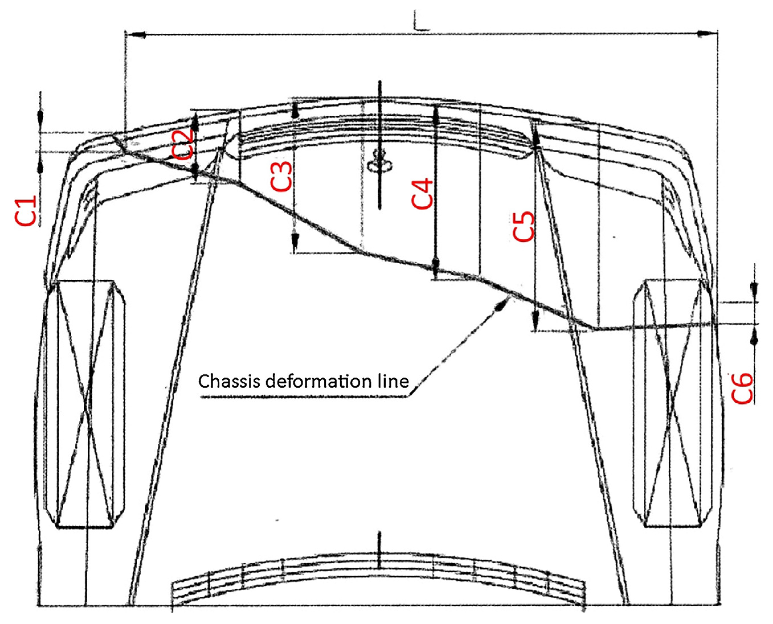
The deformation coefficient measurements are obtained according to the scheme presented in Figure 3. This explains well why adjacent measurements are so strongly correlated. The general asymmetry between coefficients C i and C 6 i for i = 1,2 , 3 is likely a result of the asymmetrical structure of reinforcing elements within the engine bay [30,31].
It should be noted that the input variables used in this study were derived from post-impact deformation measurements and therefore may be affected by measurement uncertainty resulting from damage assessment, geometric reconstruction, or observer-related variability. Such uncertainty is inherent in crash reconstruction applications and may influence the predictive accuracy of data-driven models. In the present study, no explicit uncertainty propagation procedure was applied to the input variables. Nevertheless, the use of the random forest algorithm partially mitigates the influence of local measurement errors due to its ensemble structure and relative robustness to noisy data. A formal sensitivity analysis or perturbation-based assessment of input uncertainty was beyond the scope of the present work and should be addressed in future research.

2.3. From Decision Trees to Random Forests

Decision trees are amongst the most popular methods of classification in machine learning. Their interpretability and ease of use while working with high-dimensional data make them a reliable tool with which data analysts can communicate their findings to the business and scientific world. A single decision tree is usually not enough to perform a reliable regression—it is prone to either heavy overfitting or oversimplification of the underlaying relationship between the predicted variable and predictors. This is precisely where the ensemble learning techniques come into play, as a large family of rather simple decision trees form a strong basis for a collective regression model (see Section 11 of the original paper by Breiman [33]). The random forest is obtained by building a multitude of decision trees, each trained using only a portion of the training dataset.
One of the crucial advantages of utilizing random forests is their capability to process high-dimensional data along with the quality of their predictions, even if the data is noisy or not balanced. Their immunity to distortions in data and lack of any assumptions on the feature distribution make them universal across many domains [34,35]. Additionally, their predictions are characterized by their stability, which can be further improved by increasing the number of trees (albeit this raises the computational requirements of the model as well). Lastly, random forests are particularly robust for smaller datasets with unevenly distributed variables and noise presence [36], which further reinforces our decision to utilize this particular regression technique. The bagging phenomenon [37] (Section 3.1.2) utilized intrinsically by such regressors helps with variance reduction and allows for better generalization despite the data scarcity within some input regions. To further capitalize on this, we utilize a stratified sampling strategy (as mentioned in Section 2.1 of this paper), ensuring that the training and evaluation subsets maintain a similar empirical distribution to the entire dataset.
The main drawback of the random forests is their limited interpretability. Unlike single trees or other regression models, it is hard to determine the effect of each variable on the final prediction, resulting in a phenomenon commonly described as the black-box effect. While it is possible to provide a partial explanation of the importance of each of the features in the considered dataset, following the process of generating a single prediction is tedious and, in general, lacks sense. In the subsequent paragraph, we explore certain tools [38,39,40] which allow the determination of feature importance to some extent (see also [41,42]). Despite the minor flaws we have mentioned, the random forest remains a versatile, robust method for both classification and regression tasks.

2.4. Hyperparameter Choice

For the hyperparameter tuning of the random forest, we have selected the following family of parameters:
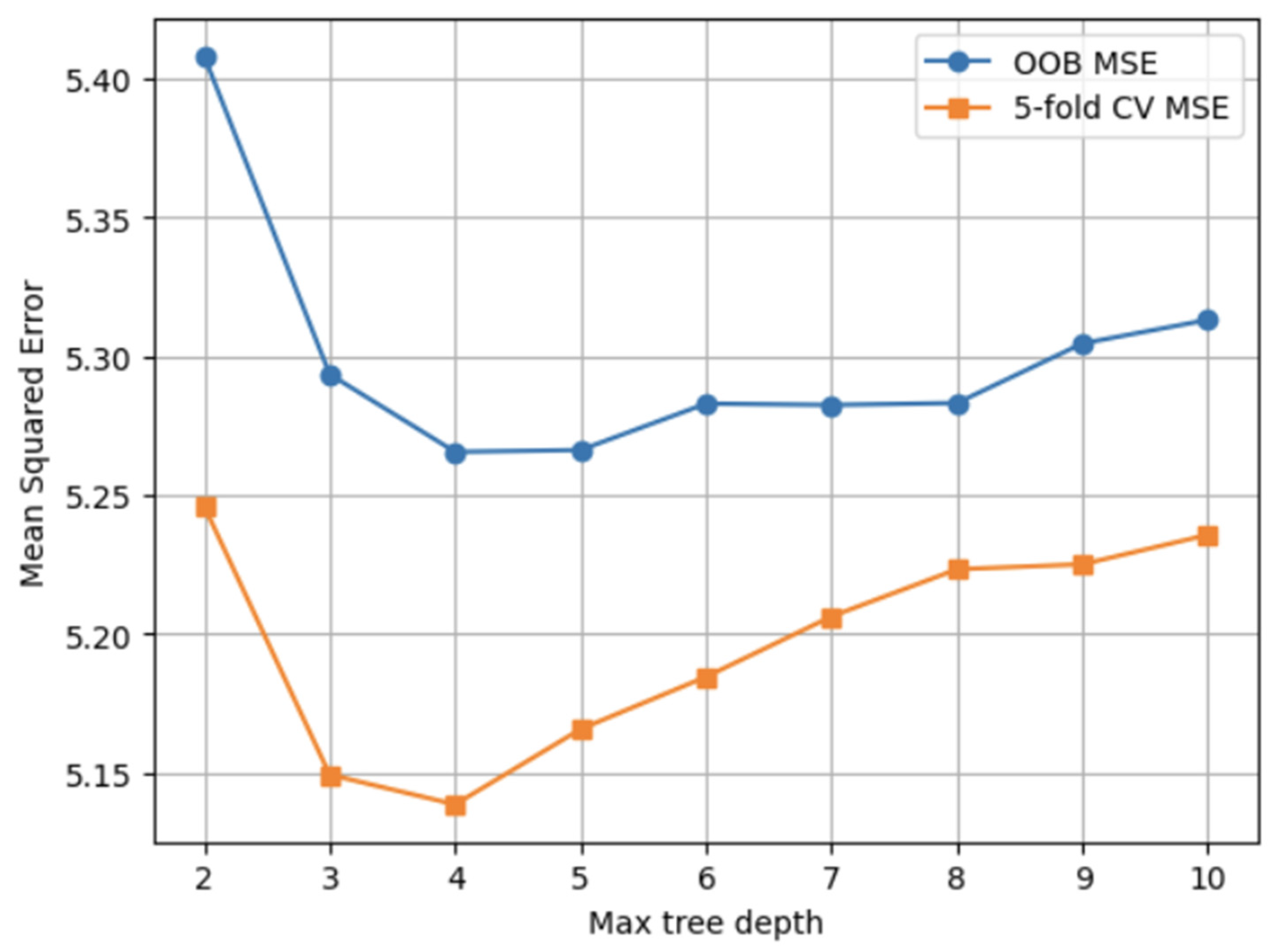
  • Maximal depth of a single tree, ranging from 4 to 20.
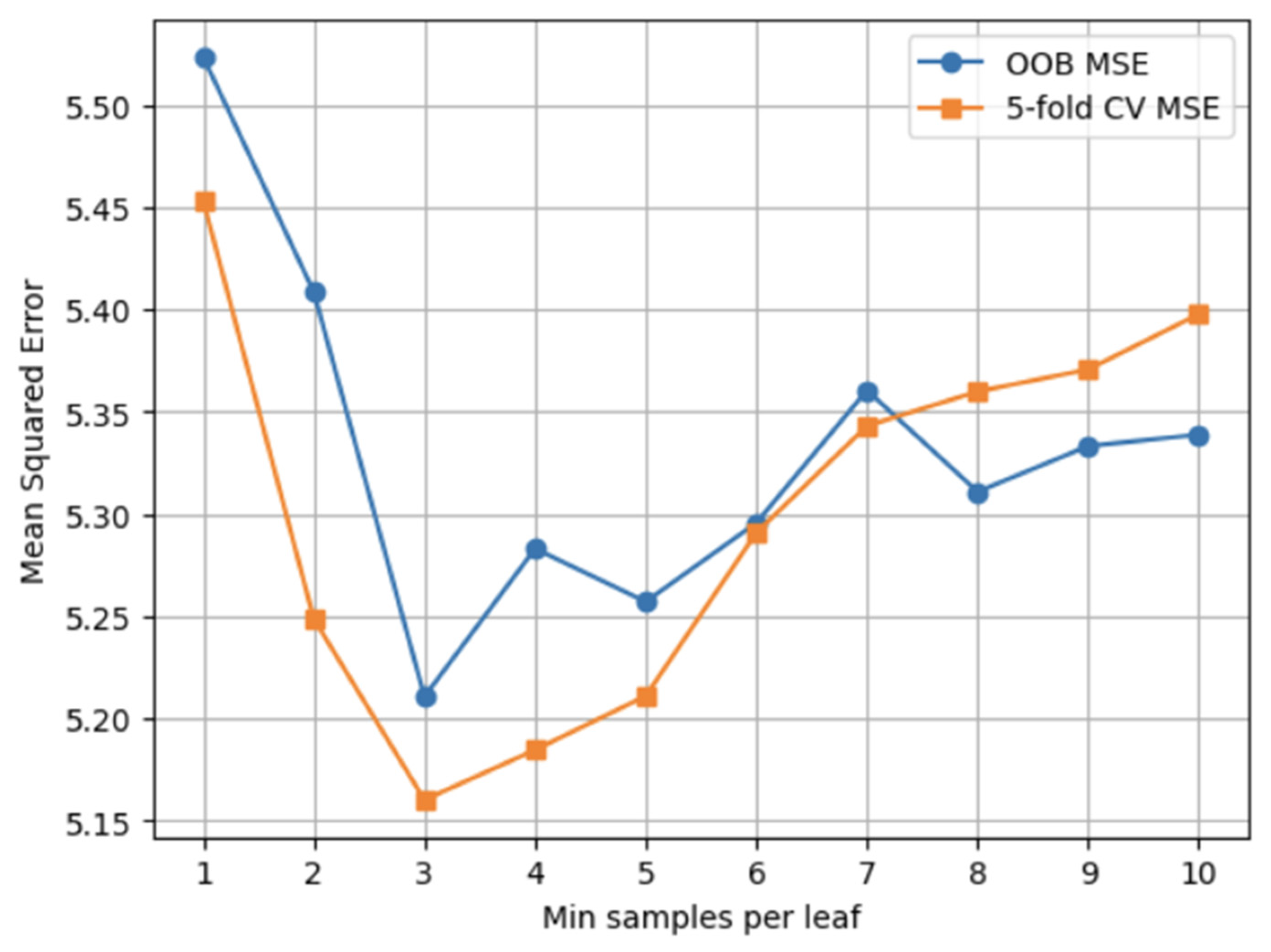
  • Minimal number of samples in the leaf, ranging between 1 and 10.
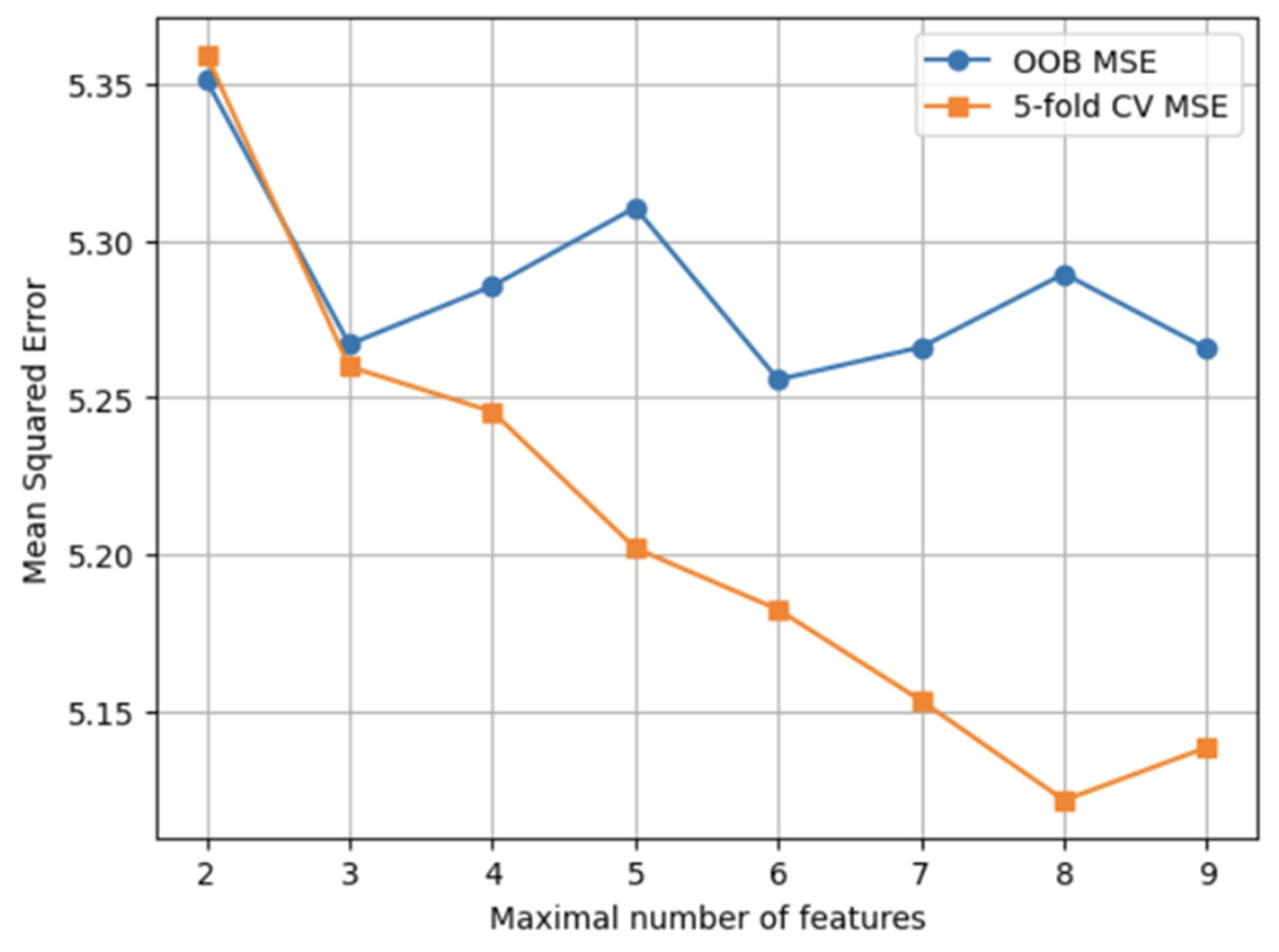
  • Maximal number of features, ranging from 2 to 9 (number of columns).
  • Minimal number of samples required to split a node, ranging from 2 to 20.
  • Number of trees, between 20 and 400, with step 10.
The selection was conducted via randomized grid search, utilizing the greedy approach. The final version of the regressor with the parameters determined via grid search utilizes:
  • Maximal depth = 6;
  • Minimal leaf = 1;
  • Maximum number of features = 9;
  • Minimal samples for split = 4;
  • 160 trees.
Interestingly, despite prominent multicollinearity of the features (in particular, C s being a linear combination of the remaining deformation values), the regressor performs best when having access to the entire array of features, as shown in Section 3. Apparently, for this task, retaining all variables leads to a more robust, reliable predictor.

2.5. Software

The numerical experiments were performed using Python (ver. 3.10), along with the numpy (ver. 1.26.4) for array-oriented computations and a selection of model-optimization tasks, sklearn (ver. 1.2.2) for the baseline regressors and scipy (ver. 1.15.3) for statistical testing. Visualizations were created using matplotlib (ver. 3.10.5) and plotly (ver. 5.18.0) modules.

3. Results

To analyze the influence of ensemble size, we observed how the error behavior changed when the number of trees varied from 20 to 400 while keeping all other hyperparameters fixed. A similar procedure was performed for the remaining parameters. For each configuration, model performance was assessed using both out-of-bag (OOB) error and five-fold cross-validation. OOB mean squared error was computed from out-of-bag predictions on the training data, while cross-validation performance was quantified using the mean squared error metric.
It is important to point out that the presented model is only applicable to the frontal full-width rigid wall scenario. The focus on this scenario is justified by the fact that the NHTSA database provides high-quality deformation data for such cases and narrowing the scenario allows for more precise predictions. By sticking to a single crash variant, we were able to construct a specialized model which works very well in such a setting, instead of obtaining a more general model which gives lower-quality predictions in a greater range of scenarios. We want to stress that for offsets of 40% or oblique collisions, re-training or changing to a different pre-crash speed estimation technique is necessary. In such cases, vehicle energy dissipation patterns may be significantly different (thus providing a highly atypical input for the model and an unreliable output as a result) when compared to the collision scenario considered within this paper.

3.1. Sensitivity Analysis

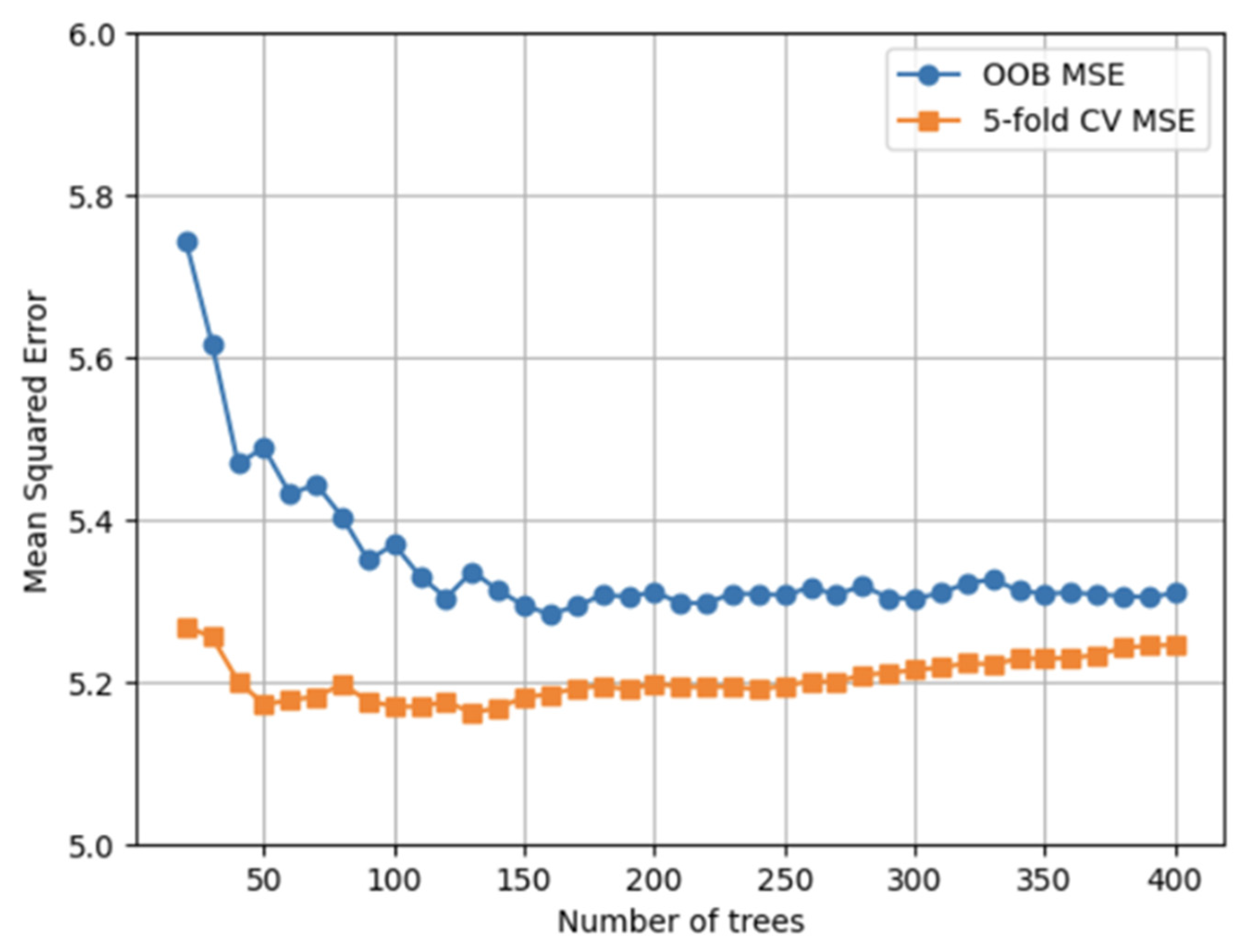
Figure 4 illustrates the dependence of prediction error on the number of trees in the random forest ensemble. Both out-of-bag (OOB) and five-fold cross-validation estimates exhibit rapid error reduction for small ensemble sizes, followed by clear stabilization beyond approximately 150 trees. The close agreement between OOB and cross-validation curves indicates consistent generalization performance and suggests that further increasing the number of trees does not yield meaningful accuracy improvements.
Analyzing the behavior of the error function for varying minimal leaf size (see Figure 5) yields several important corollaries. A clear optimum is obtained for relatively small leaf sizes—a requirement for a minimum of 3–5 samples per leaf yields the lowest error values. Increasing this further leaves us with a model which shows clear signs of underfitting—the individual trees become too shallow, and subsequently, the random forest loses its ability to model local substructures of the underlying data distribution. On the other hand, very small leaves yield a moderate risk of overfitting, despite the variance reduction stemming from the ensemble learning technique itself. The stable error behavior around the selected minimal leaf size indicates that the model is not extremely sensitive in this region of hyperparameter space.
Similar observations can be made about the limitations on the maximal tree depth. A risky region indicating possible overfitting starts when the limit starts to exceed 5–6. Trees of depth 2 are too shallow for any meaningful inference, which leaves us with a relatively stable error region for maximal depth ranging between 3 and 5. Figure 6 therefore depicts the natural variance–bias trade-off which can be observed for this regressor.
Lastly, Figure 7 depicts the relationship between the number of features utilized by a single tree and the overall quality of the obtained random forest regressor. In general, from the plot, we can observe that the best results are obtained if the entire (possibly missing a single feature) collection of features is utilized by each tree. In this plot, a 5-fold CV error decrease can be observed, indicating overall improvement of the model with increased access to the distinct predictors by individual trees. The fluctuations in OOB error indicate possible mild heterogeneity in feature importance across the subsamples selected for the training process.
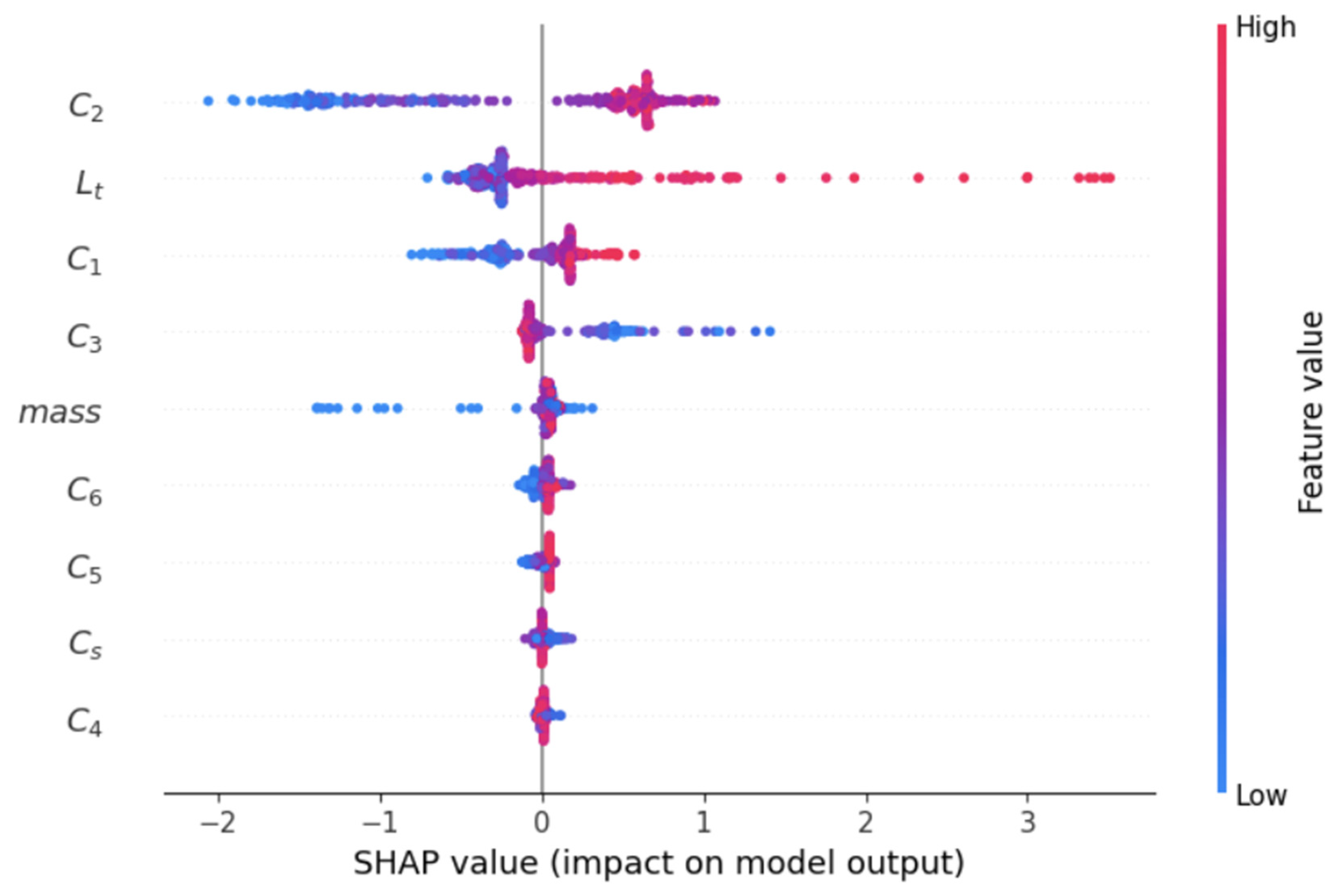
As far as interpretability of the model is concerned, we utilized two approaches to counter the black-box nature of the random forest regressor to a certain extent. First, we used the Shapley Additive Explanations (SHAP values) to identify how much the final model relies on each of the features utilized in predictions. As Figure 8 shows, the model’s behavior is mainly driven by the left-hand side of the impact (features C 1 , C 2 , C 3 as well as impact zone width L t ). This remains consistent with physical experience, where the deformation is the strongest predictor. What is surprising is the fact that C 3 seems to be acting as a counterbalance to the remaining factors. Also, the mass of the vehicle seems to be important mainly in cases where it strongly deviates from the mean value for the car class considered.
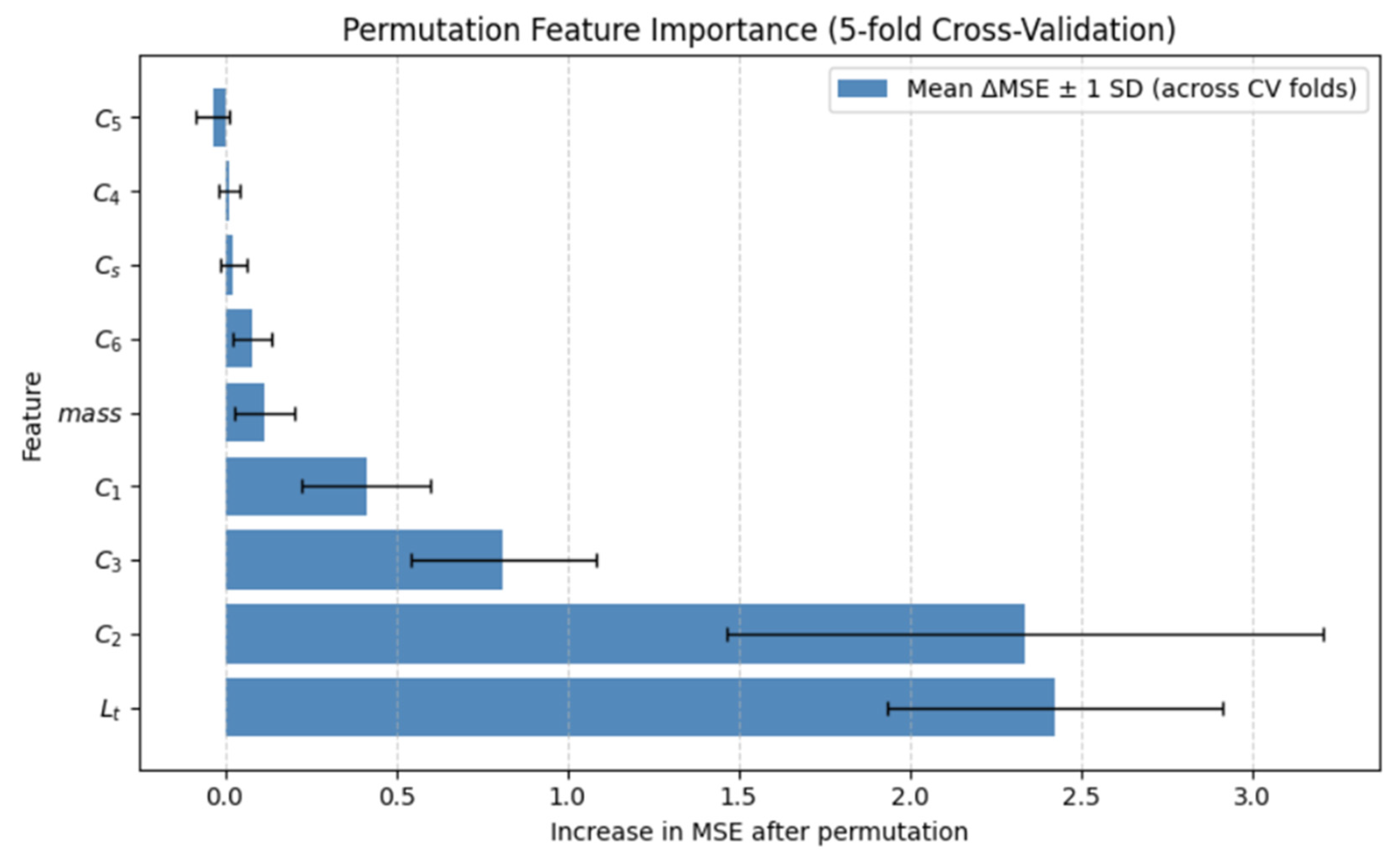
These observations are subsequently confirmed by calculation of the permutation feature importance (see [38] (Section 5.2); also see [39,40]). In general, permutation feature importance (PFI) is a model-agnostic way to measure how much each input feature contributes to a model’s predictive performance. Conceptually, a feature is considered important if, when its values are randomly permuted (shuffled) in a test set —thus breaking its relationship with the target—the model’s error gets noticeably worse. More formally, for a fixed trained model, PFI for feature X j is defined as the increase in expected loss when X j is replaced by an independently permuted copy that preserves its marginal distribution but destroys its association with the target and other features. Larger values of PFI mean that the model’s performance degrades more when that feature is permuted, thus indicating how significant the given variable is for the final prediction quality. In Figure 9, we can observe the PFI values for all features (the 5-fold CV was used to remove the randomness impact). The features C 4 , C 5 , C 6 , C S and m a s s are not of major significance for the model, with the C 5 coefficient most likely being a rather noisy feature. In particular, the impact of C 5 is naturally mitigated by the inner mechanisms of the RF regressor, which clearly favors other, more stable predictors. The features C 2 and L t are the major players in the final outcome quality, as permuting them increases MSE most significantly. The two remaining features, C 3 and C 1 , seem to also be of high importance, but they contribute significantly less than the former two. These observations are consistent with the corollaries drawn from the SHAP value analysis.

3.2. Comparison with Basic Linear Model

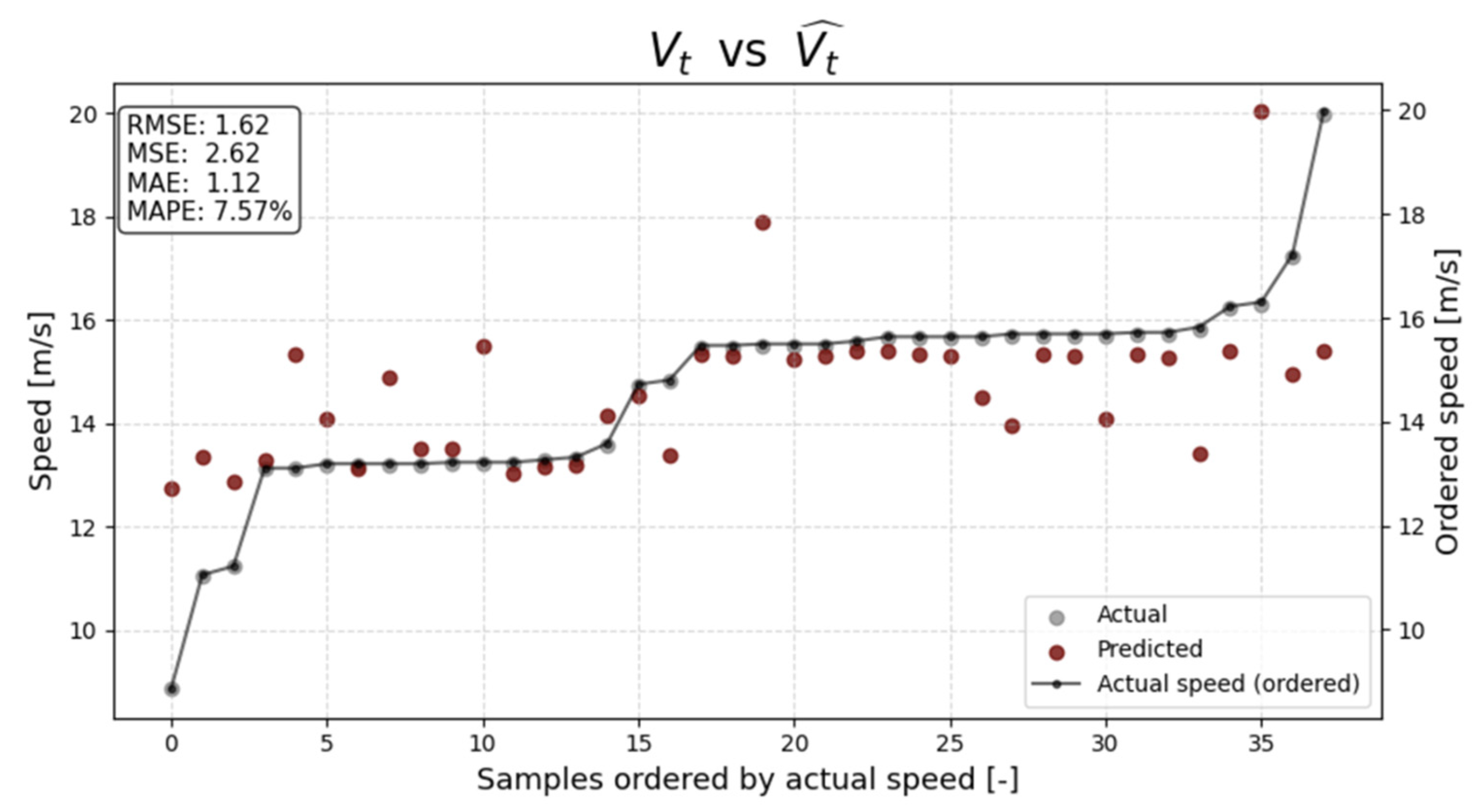
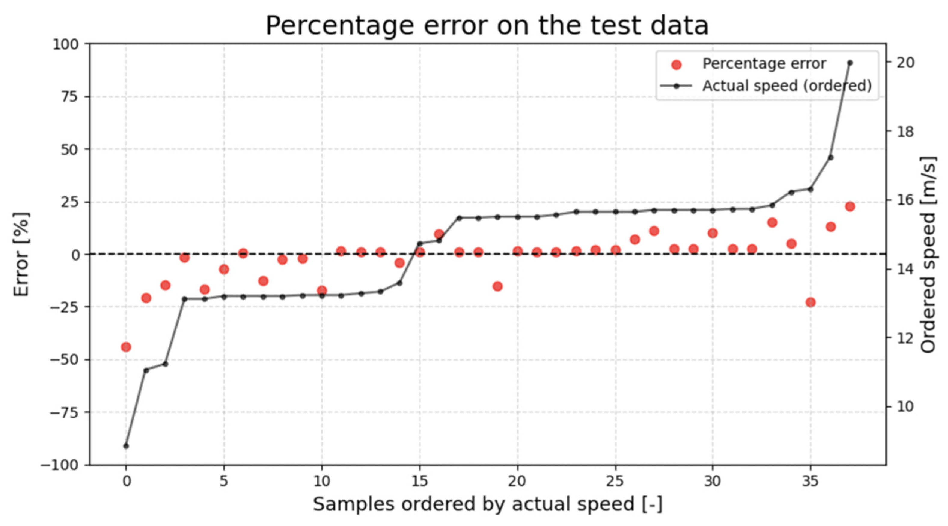
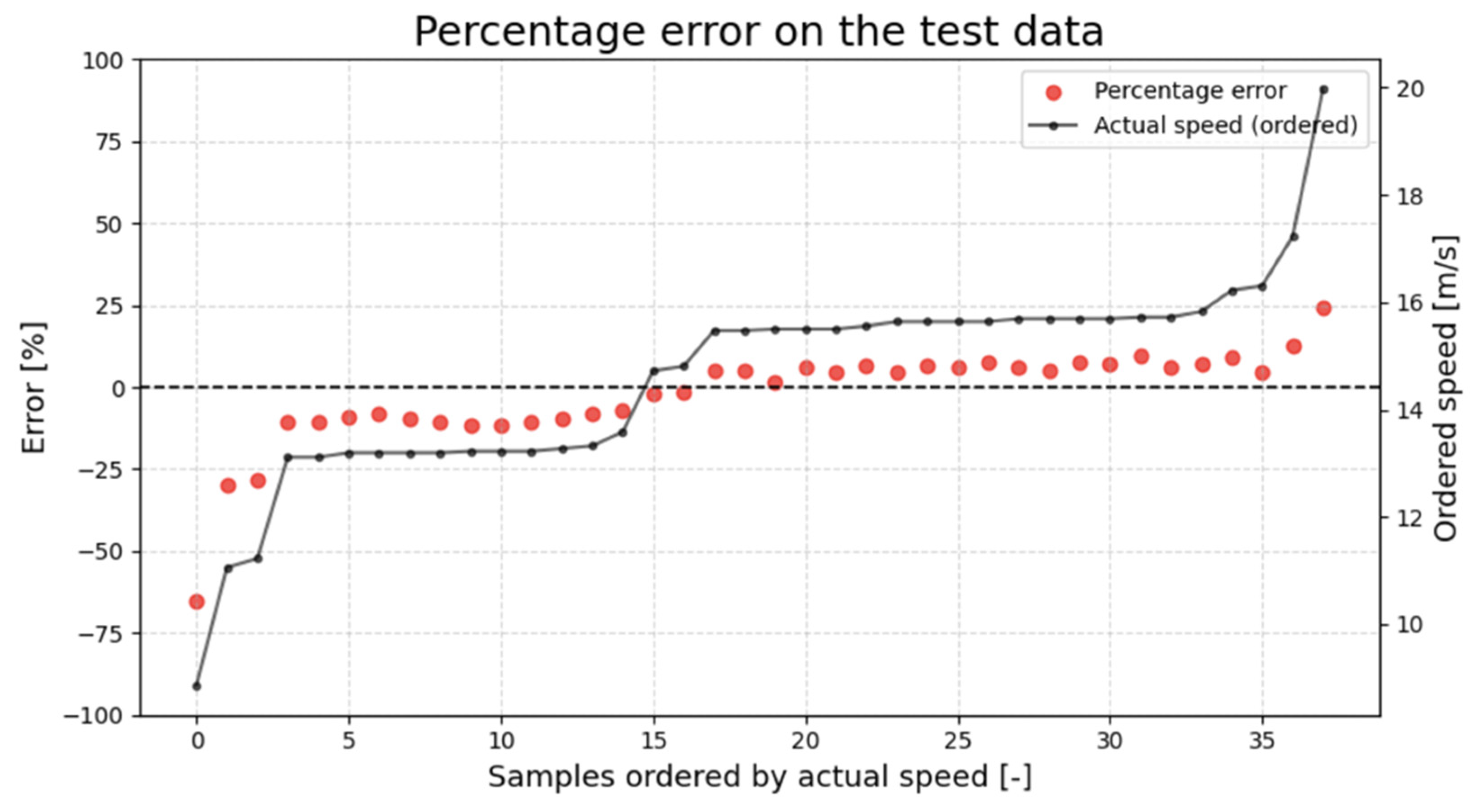
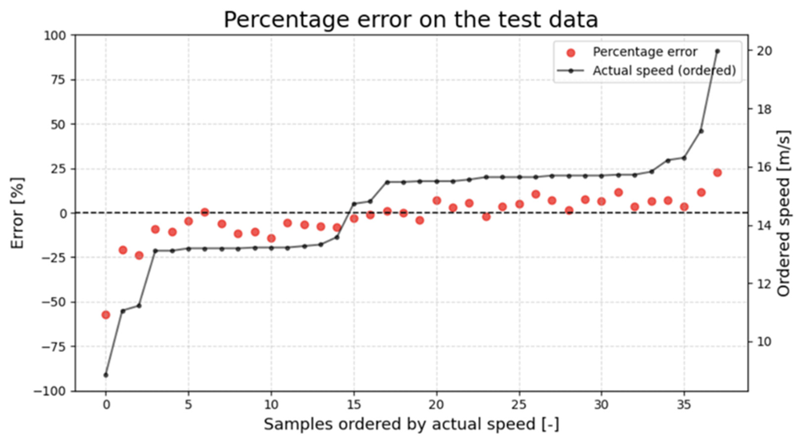
The obtained model was then compared against the linear model on a test set. The results are graphically presented in Figure 10, Figure 11, Figure 12 and Figure 13. The tabular summary from the test set can be found in Table 2.
Overall, the model has attained stratified MAPE slightly above 7.5%, which corresponds to a mean absolute error around 1.12   m / s with a root mean squared error of 1.62   m / s .
For comparison, the linear regression with regularization yields nearly 10 % error, which corresponds to an RMSE of nearly 1.70   m / s and a mean average error of 1.42   m / s .
An additional advantage of the RF-based model over classical approaches is prominent here—due to the nature of the random forest training, the feature subsampling (selection of a single feature at each computation step) handles multicollinearity automatically.
As we can see, the model based on linear regression has noticeable problems with the observations which lay outside of the range from 13 to 15   m / s . This accurately represents the main weakness of linear regression, which is the lack of ability to properly handle values which rarely occur in the dataset and tend to deviate to regions where observations are sparse. On the other hand, the linear approximation error seems to behave more consistently in comparison to the random forest approximation.
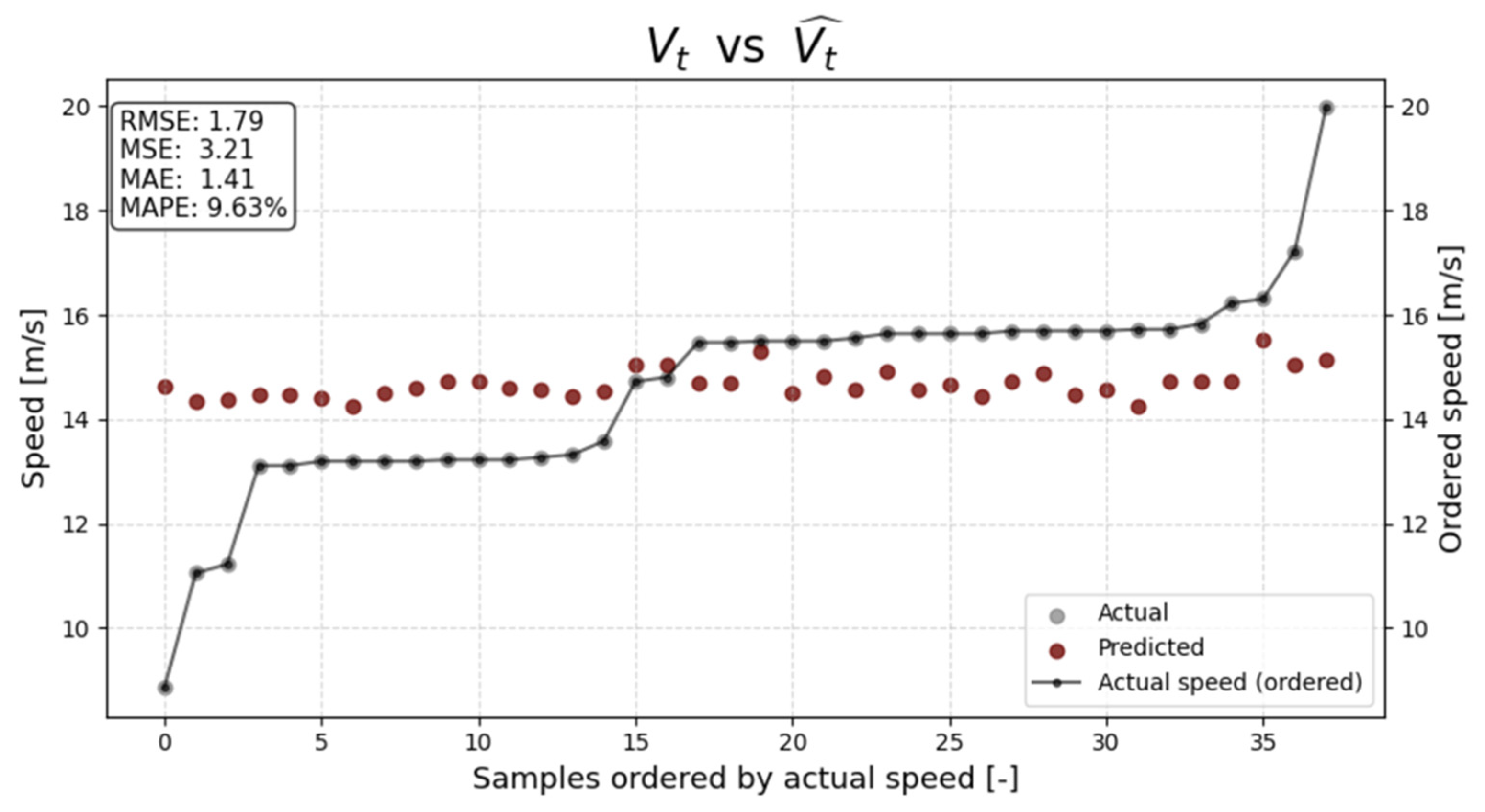
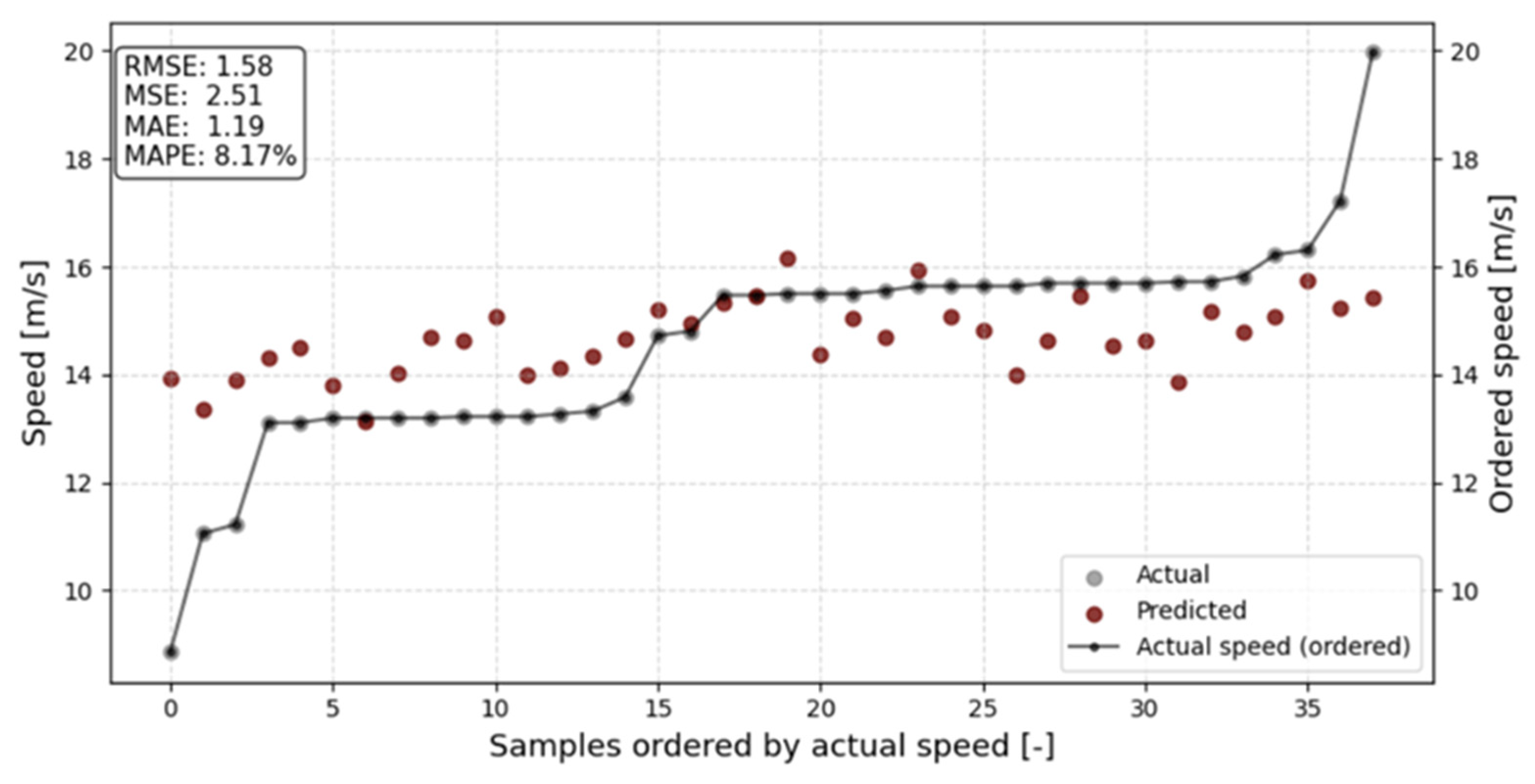
For subsequent (and more fair) comparison, a simple single-layer neural network was trained, consisting of 15 neurons using ReLU as an activation function. While such a perceptron approach largely outperforms the linear model (with MAPE as low as 8.17 % and corresponding MAE 1.19   m / s ), it is still not as efficient as the random forest approach. Detailed results are included in Figure 14 and Figure 15 below.
Lastly, as suggested by one of the anonymous reviewers, we performed a comparison of our regressor against more modern gradient-boosted tree ensembles. In general, they provided no significant accuracy gains over random forest—this is most likely caused by the modest size of this specific dataset. The overall greater predictive power of XGBoost and LightGBM approaches has proven very difficult to extract in this scenario even with careful fine-tuning, as the resulting classifiers are much more prone to overfitting (a brief comparison is provided in Table 3 below, with our random forest predictor included for juxtaposition).
To improve the reliability of model evaluation, predictive performance was not interpreted solely on the basis of a single train–test split. In addition to the hold-out test set, model stability was assessed using 5-fold cross-validation and out-of-bag estimation for the random forest model. This complementary evaluation strategy reduces the risk of overinterpreting results obtained from a relatively small test subset and provides a more robust basis for comparing predictive performance across the analyzed methods.

4. Discussion and Conclusions

Interpreting the obtained results from an energy systems perspective, the proposed random forest-based approach demonstrates a high capability to reconstruct the effective kinetic energy dissipated during frontal impacts. The achieved accuracy indicates that deformation-derived energy indicators contain sufficient information to reliably estimate pre-crash velocity, even in the absence of direct onboard energy or speed measurements.
This finding is particularly relevant for energy-aware vehicle safety research, as it confirms that empirical, data-driven models can complement classical energy balance formulations while maintaining practical applicability under real-world conditions.
The proposed model is amongst the best models known in the literature. For comparison,
  • FEM approaches suggested in [32] yield error values ranging from 1.19% to 4.29%. However, these methods require significantly more data and computational power and were tested mainly via simulations. For comparison, the RF-based model presented in this paper does not require any stiffness analysis of the vehicle under consideration (although such data could possibly be used to improve the regressor substantially).
  • In comparison with FEM techniques [32], all the data necessary for pre-crash velocity estimation can be gathered from the accident site. The deformation measurements along with vehicle mass are easy to both obtain and instantly process via the pre-trained regressor, while finite element methods are much more effort- and time-consuming, without providing a truly significant advantage.
  • In [43], the authors’ work on Legendre polynomials for the compact class yields relative error rates ranging between 6.3% and 6.74%; similar level of accuracy is obtained via usage of tensor-product or B-spline approaches shown in [18]. It is important to point out that the latter paper uses weighted error measurements; i.e., the weight of each error corresponds to the typicality of the observation. The unweighted, stratified approach for the error measurements therein yielded slightly worse results (with MAPE 8.02%).
The energy-based approach to pre-crash velocity prediction of the method proposed in the scope of this article can also be applied to other car classes to further enhance the precision of accident reconstruction techniques. What is important is that the presented model has practical and field-applicable characteristics, making it suitable for use in real collision scenarios. This is especially important in the case of older vehicles, which lack Event Data Recorders. Therefore, the random forest approach presented in this paper provides a low-cost alternative to more computationally intensive techniques for forensics.

Further Research

Broadly speaking, the compact car class had not been explored properly in the literature until now. Similarly (to the best of the authors’ knowledge), there is no recorded application of ensemble learning techniques applied to pre-crash velocity estimation. This paper is dedicated to filling this research gap and does so with satisfying results. To enable broader validation, we plan to further analyze the compact class of the NHTSA crash-test database. Access to an expanded dataset could provide support for a more comprehensive evaluation of the method’s performance.
Further directions for research include:
  • Experimental feature reconstruction, involving the impact deflection angle (which can possibly be inferred from the deformation coefficients Ci and the relationship between these).
  • Preparation of an analogous model based on the data collected from EDRs from modern vehicles.
  • Including feature engineering via preliminary stiffness analysis in applicable cases.
From the viewpoint of sustainable mobility and energy-efficient vehicle design, future research may also explore the relationship between reconstructed pre-crash energy levels and structural energy absorption efficiency across different vehicle classes. Such analyses could support the evaluation of lightweight materials and alternative structural concepts with respect to their real-world energy dissipation performance during collisions.
The results of this study should be interpreted in light of several limitations. First, the developed model was trained and validated exclusively on crash-test data for compact passenger cars involved in full-width frontal impacts against a rigid barrier. Consequently, the proposed approach should not be directly generalized to other vehicle classes or to different crash configurations, such as offset, oblique, or vehicle-to-vehicle impacts, without further validation. Second, the dataset used in this study was relatively small and imbalanced, with most observations concentrated in a limited velocity range, which may affect predictive performance for less represented cases. Third, the input variables were derived from post-impact deformation measurements, and the accuracy of the predictions therefore depends on the quality and consistency of the measured damage parameters. Finally, although random forest is relatively robust to noise and overfitting, this study did not include a formal uncertainty propagation or sensitivity analysis, which should be considered in future work.

Author Contributions

Conceptualization, P.K., F.T., M.P. and M.M.; methodology, B.L., F.T. and M.P.; software, B.L., M.P. and M.M.; validation, F.T., M.P. and D.F.; formal analysis, B.L. and M.P.; investigation, F.T., B.L. and M.P.; resources, P.K. and M.P.; data curation, P.K., M.P. and J.J.; writing, original draft preparation, F.T. and M.P.; writing, review and editing, P.K., M.P. and M.J.; visualization, B.L., F.T. and M.P.; supervision, F.T. and M.P.; project administration, P.K. and M.P. All authors have read and agreed to the published version of the manuscript.

Funding

This work was supported by the Slovak Research and Development Agency under the Contract no. SK-CN-23-0009 “Dynamic Modeling and Management of Car-Bicycle Mixed Traffic Flow in Intelligent Connected Vehicle Environment”.

Data Availability Statement

While the data itself is publicly available from NHTSA website, the extracted and initially preprocessed version of the crash reports information utilized in the experiment is available publicly at https://doi.org/10.5281/zenodo.18873884.

Acknowledgments

The authors would like to acknowledge the anonymous reviewers from the initial and final submissions for all the suggestions and comments which led to increased overall quality of the paper. This article was completed while the second author worked in the Interdisciplinary Doctoral School at the Lodz University of Technology, Poland. Filip Turoboś is supported by the National Science Center (NCN), Poland, project: Sonata Bis 10, No. 2020/38/E/ST3/00269 (B.G).

Conflicts of Interest

The authors declare no conflicts of interest.

Abbreviations and Symbols

The following abbreviations and symbols are used in this manuscript:
EESEquivalent Energy Speed [ m / s ]
NHTSANational Highway Traffic Safety Administration
C 1 C 6 deformation coefficients [ m ]
C s average deformation coefficient [ m ]
V t vehicle speed [ m / s ]
m a s s mass of car [ k g ]
L t deformation zone width [ m ]
N = 399number of cases [ ]
M R S E Mean Root-Square Error [ m / s ]
M A P E Mean Absolute Percentage Error [ % ]
M A E Mean Absolute Error [ m / s ]
M S E Mean Squared Error [ m 2 / s 2 ]

References

  1. Gaj, P.; Kopania, J.; Wójciak, K.; Bogusławski, G. Assessment of sound absorbing properties of composite made of recycling materials. Vib. Phys. Syst. 2019, 30, 2019109. [Google Scholar]
  2. Bukvić, M.; Milojević, S.; Gajević, S.; Đorđević, M.; Stojanović, B. Production Technologies and Application of Polymer Composites in Engineering: A Review. Polymers 2025, 17, 2187. [Google Scholar] [CrossRef]
  3. Wójciak, K.; Kopania, J.M. Correlation Between the Shape of Substitution Ducts and Insertion Loss of Silencers. Vib. Phys. Syst. 2022, 33, 2022212. [Google Scholar] [CrossRef]
  4. Campbell, K.L. Energy Basis for Collision Severity; SAE Technical Paper 740565; SAE: Warrendale, PA, USA, 1974. [Google Scholar] [CrossRef]
  5. Brach, R.M.; Brach, R.M. Crush Energy and Planar Impact Mechanics for Accident Reconstruction; SAE Technical Paper 980025; SAE: Warrendale, PA, USA, 1998. [Google Scholar] [CrossRef]
  6. Rose, N.A. Restitution Modeling for Crush Analysis: Theory and Validation; SAE Technical Paper 2006-01-0908; SAE: Warrendale, PA, USA, 2006. [Google Scholar] [CrossRef]
  7. Brach, R.M.; Brach, R.M.; Mink, R.A. Nonlinear Optimization in Vehicular Crash Reconstruction. SAE Int. J. Transp. Saf. 2015, 3, 17–27. [Google Scholar] [CrossRef]
  8. Mrowicki, A.; Krukowski, M.; Turoboś, F.; Jaśkiewicz, M.; Radkowski, S.; Kubiak, P. Determining vehicle pre-crash speed in frontal barrier crashes using genetic algorithm model adjustment techniques for intermediate car class. Int. J. Crashworthiness 2021, 27, 1009–1016. [Google Scholar] [CrossRef]
  9. Mrowicki, A.; Krukowski, M.; Turoboś, F.; Kubiak, P. Determining vehicle pre-crash speed in frontal barrier crashes using artificial neural network for intermediate car class. Forensic Sci. Int. 2020, 308, 110179. [Google Scholar] [CrossRef] [PubMed]
  10. Bayarri, M.J.; Berger, J.O.; Kennedy, M.C.; Kottas, A.; Paulo, R.; Sacks, J.; Cafeo, J.A.; Lin, C.-H.; Tu, J. Predicting Vehicle Crashworthiness: Validation of Computer Models for Functional and Hierarchical Data. J. Am. Stat. Assoc. 2009, 104, 929–943. [Google Scholar] [CrossRef]
  11. Wang, X.; Shi, L. A new metamodel method using Gaussian process based surrogate modeling for crashworthiness design. Int. J. Crashworthiness 2014, 19, 311–321. [Google Scholar] [CrossRef]
  12. Eilers, P.H.C.; Marx, B.D. Flexible Smoothing with B-splines and Penalties. Stat. Sci. 1996, 11, 89–121. [Google Scholar] [CrossRef]
  13. Piegl, L.; Tiller, W. The NURBS Book, 2nd ed.; Springer: Berlin/Heidelberg, Germany, 1997. [Google Scholar]
  14. Neades, J.; Smith, R. The determination of vehicle speeds from delta-V in two vehicle planar collisions. Proc. Inst. Mech. Eng. Part D J. Automob. Eng. 2011, 225, 43–53. [Google Scholar] [CrossRef]
  15. Doecke, S.D.; Dutschke, J.K.; Baldock, M.R.J.; Kloeden, C.N. Travel speed and the risk of serious injury in vehicle crashes. Accid. Anal. Prev. 2021, 161, 106359. [Google Scholar] [CrossRef]
  16. Spek, A.; Otjens, J. Understanding pre-crash speed sampling by the VAG Event Data Recorder. Forensic Sci. Int. 2023, 351, 111831. [Google Scholar] [CrossRef]
  17. Breitlauch, P.; Erbsmehl, C.T.; van Ratingen, M.; Mallada, J.L.; Sandner, V.; Ferson, N.; Urban, M. A novel method for the automated simulation of various vehicle collisions to estimate crash severity. Traffic Inj. Prev. 2023, 24, 116–123. [Google Scholar] [CrossRef]
  18. Poliak, M.; Kubiak, P.; Krukowski, M.; Turoboś, F.; Jaśkiewicz, M.; Jaśkiewicz, J.; Frej, D. Non-Linear Method of Vehicle Velocity Determination Based on Tensor Product B-Spline Approximation with Probabilistic Weights for NHTSA Database of Compact Vehicle Class. Appl. Sci. 2026, 16, 401. [Google Scholar] [CrossRef]
  19. Bruski, D.; Pachocki, L.; Sciegaj, A.; Witkowski, W. Speed estimation of a car at impact with a W-beam guardrail using numerical simulations and machine learning. Adv. Eng. Softw. 2023, 184, 103502. [Google Scholar] [CrossRef]
  20. Silver, D.; Manek, H.; Kay, M.; Travis, P. Estimating Automobile Crash Characteristics from Images using Deep Learning. In Proceedings of the International FLAIRS Conference Proceedings, Clearwater Beach, FL, USA, 14–17 May 2022; The Florida Artificial Intelligence Research Society: Coral Gables, FL, USA, 2022; Volume 35. [Google Scholar] [CrossRef]
  21. Thapa Magar, A.; Osthi, S.; Adhikari, N.; Saban Kumar, K.C. Multi-model Deep Learning Approaches for Vehicle Speed Estimation. Kathford J. Eng. Manag. 2025, 4, 21–30. [Google Scholar] [CrossRef]
  22. Fernández Llorca, D.; Hernández Martínez, A.; García Daza, I. Vision-based vehicle speed estimation: A survey. IET Intelligent Transport Systems 2021, 15, 987–1005. [Google Scholar] [CrossRef]
  23. Famouri, M.; Azimifar, Z.; Wong, A. A Novel Motion Plane-Based Approach to Vehicle Speed Estimation. IEEE Trans. Intell. Transp. Syst. 2019, 20, 1237–1246. [Google Scholar] [CrossRef]
  24. Gulino, M.; Di Gangi, L.; Sortino, A.; Vangi, D. Injury risk assessment based on pre-crash variables: The role of closing velocity and impact eccentricity. Accid. Anal. Prev. 2020, 150, 105864. [Google Scholar] [CrossRef] [PubMed]
  25. Andricevic, N.; Junge, M.; Krampe, J. Injury risk functions for frontal oblique collisions. Traffic Inj. Prev. 2018, 19, 518–522. [Google Scholar] [CrossRef]
  26. Ameksa, M.; Mousannif, H.; Al Moatassime, H.; Elamrani Abou Elassad, Z. Crash Prediction using Ensemble Methods. In Proceedings of the 2nd International Conference on Big Data, Modelling and Machine Learning—BML, Kenitra, Morocco, 15–16 July 2021; SciTePress: Setúbal, Portugal, 2022; pp. 211–215. ISBN 978-989-758-559-3. [Google Scholar] [CrossRef]
  27. Lin, L.; Wang, Q.; Sadek, A.W. A novel variable selection method based on frequent pattern tree for real-time traffic accident risk prediction. Transp. Res. C Emerg. Technol. 2015, 55, 444–459. [Google Scholar] [CrossRef]
  28. Islam, Z.; Abdel-Aty, M.; Anik, B.M.T.H. Transformer-Conformer Ensemble for Crash Prediction Using Connected Vehicle Trajectory Data. IEEE Open J. Intell. Transp. Syst. 2023, 4, 979–988. [Google Scholar] [CrossRef]
  29. Wu, P.; Meng, X.; Song, L. A novel ensemble learning method for crash prediction using road geometric alignments and traffic data. J. Transp. Saf. Secur. 2020, 12, 1128–1146. [Google Scholar] [CrossRef]
  30. National Highway Traffic Safety Administration (NHTSA). CRASH3 User’s Guide and Technical Manual; Report No. DOT HS 805 732; National Highway Traffic Safety Administration: Washington, DC, USA, 1982.
  31. Lindquist, M.; Hall, A.; Björnstig, U. Real world car crash investigations—A new approach. Int. J. Crashworthiness 2003, 8, 375–384. [Google Scholar] [CrossRef]
  32. Droździel, P.; Pasaulis, T.; Pečeliūnas, R.; Pukalskas, S. Evaluation of the Energy Equivalent Speed of Car Damage Using a Finite Element Model. Vehicles 2024, 6, 632–650. [Google Scholar] [CrossRef]
  33. Breiman, L. Random Forests. Mach. Learn. 2001, 45, 5–32. [Google Scholar] [CrossRef]
  34. Salman, H.A.; Kalakech, A.; Steiti, A. Random Forest Algorithm Overview. Babylon. J. Mach. Learn. 2024, 2024, 69–79. [Google Scholar] [CrossRef]
  35. Schonlau, M.; Zou, R.Y. The random forest algorithm for statistical learning. Stata J. 2020, 20, 3–29. [Google Scholar] [CrossRef]
  36. Roy, M.H.; Larocque, D. Robustness of random forests for regression. J. Nonparametric Stat. 2012, 24, 993–1006. [Google Scholar] [CrossRef]
  37. Genuer, R.; Poggi, J.M. Random Forests. In Random Forests with R; Use R! Springer: Cham, Switzerland, 2020. [Google Scholar] [CrossRef]
  38. Mandler, H.; Weigand, B. A review and benchmark of feature importance methods for neural networks. ACM Comput. Surv. 2024, 56, 318. [Google Scholar] [CrossRef]
  39. Fisher, A.; Rudin, C.; Dominici, F. All models are wrong, but many are useful: Learning a variable’s importance by studying an entire class of prediction models simultaneously. J. Mach. Learn. Res. 2019, 20, 1–81. [Google Scholar]
  40. Molnar, C.; König, G.; Bischl, B.; Casalicchio, G. Model-agnostic feature importance and effects with dependent features: A conditional subgroup approach. Data Min. Knowl. Disc. 2024, 38, 2903–2941. [Google Scholar] [CrossRef]
  41. Ishwaran, H.; Lu, M. Standard errors and confidence intervals for variable importance in random forest regression, classification, and survival. Stat. Med. 2018, 38, 558–582. [Google Scholar] [CrossRef] [PubMed]
  42. Speiser, J.L.; Miller, M.E.; Tooze, J.; Ip, E. A Comparison of Random Forest Variable Selection Methods for Classification Prediction Modeling. Expert Syst. Appl. 2019, 134, 93–101. [Google Scholar] [CrossRef] [PubMed]
  43. Kubiak, P.; Mierzejewska, P.; Krukowski, M. Nonlinear methods of vehicle velocity determination based on inverse systems and tensor products of Legendre polynomials in compact car class. Forensic Sci. Int. 2018, 295, 19–29. [Google Scholar] [CrossRef]
Figure 1. A scatterplot of observations within the dataset, displaying C s   [ m ] ,   m a s s   [ k g ] and V t m s .
Energies 19 01678 g001
Figure 2. Pearson correlation between features.
Energies 19 01678 g002
Figure 3. Measurement method of coefficients from C 1 to C 6 (see also Figure 3 in [32]).
Energies 19 01678 g003
Figure 4. The relationship between observed mean squared error and the number of trees. The fluctuations in error behavior stabilized after exceeding 150–160 trees.
Energies 19 01678 g004
Figure 5. MSE dependency on the choice of hyperparameter defining the minimal number of samples per leaf.
Energies 19 01678 g005
Figure 6. Sensitivity analysis of the maximal tree depth hyperparameter.
Energies 19 01678 g006
Figure 7. Sensitivity analysis of the maximal number of features utilized by a single tree.
Energies 19 01678 g007
Figure 8. SHAP values for the resulting model.
Energies 19 01678 g008
Figure 9. Permutation feature importance for the resulting model.
Energies 19 01678 g009
Figure 10. Plot depicting random forest predictions and actual pre-crash speeds on the test set.
Energies 19 01678 g010
Figure 11. Plot depicting random forest prediction errors (percentage) for test set examples.
Energies 19 01678 g011
Figure 12. Plot depicting linear regression predictions and actual pre-crash speeds on the test set.
Energies 19 01678 g012
Figure 13. Plot depicting linear regression prediction percentage errors on the test set.
Energies 19 01678 g013
Figure 14. Plot of neural network predictions for the test set.
Energies 19 01678 g014
Figure 15. Plot of neural network prediction errors (percentage) for the test set.
Energies 19 01678 g015
Table 1. Basic statistical characteristics of the data.
S t a t i s t i c C 1   [ m ] C 2   [ m ] C 3   [ m ] C 4   [ m ] C 5   [ m ] C 6   [ m ] C s   [ m ] L t   [ m ] m a s s   [ k g ] V t m s
m e a n 0.4390.4820.4910.4670.4300.3860.4561.4961364.72914.679
s t d 0.1820.1570.1560.1590.1610.1650.1420.14461.092.574
m i n 0.0380.0920.0930.0490.0790.0150.1031.051251.04.472
Q 25 %   0.3140.3760.3830.3630.3090.2450.3621.4001324.013.222
Q 50 %   0.4320.4800.4950.4750.4370.3840.4551.4991363.015.5
Q 75 %   0.5430.5660.5800.5710.5370.5080.5431.5861410.515.694
m a x 1.3671.2901.3361.3491.3561.3441.3281.9141478.026.861
Table 2. A comparison of linear and random forest regression estimations on the selected part of the test set. Bold font for each row denotes better approximation.
C s   [ m ] L t   [ m ] m a s s   [ k g ] V t   [ m / s ] Linear   Prediction   [ m / s ] Linear Method
Absolute
Error [ m / s ]
Linear Method
Relative
Error [ % ]
Random Forest
Prediction [ m / s ]
Random
Forest
Absolute
Error [ m / s ]
Random
Forest
Relative
Error [ % ]
0.381.370126311.0614.353.3029.8413.342.2820.65
0.381.425142313.1114.491.3810.5013.290.181.38
0.671.321128415.7214.241.499.4515.330.402.52
0.481.524136916.2214.731.499.2115.400.825.05
0.541.417140213.1114.471.3610.3615.322.2116.83
0.101.658136814.8115.050.251.6813.371.449.71
0.281.380147511.2214.383.1628.1312.861.6414.64
0.491.565132215.5014.830.674.3415.310.191.26
0.281.322132113.1914.241.047.9113.140.060.43
0.431.401146513.3214.431.118.3213.190.131.01
0.701.461125115.6914.581.127.1314.091.6010.22
0.541.524140615.7214.730.996.3215.280.442.79
0.641.511142915.4714.700.785.0115.330.140.93
0.521.455139715.5614.560.996.3915.390.171.10
0.411.473143713.1914.601.4110.6913.520.332.50
0.281.452138913.2714.551.289.6613.140.130.96
0.261.658136417.2215.052.1712.5914.952.2713.17
0.231.658136314.7215.050.332.2514.550.181.19
0.551.420140715.6914.481.227.7615.290.402.58
0.291.524146515.8214.731.106.9313.402.4315.33
0.461.427128013.1914.491.309.8414.891.7012.87
0.601.499131615.6414.670.976.2115.310.332.11
0.291.48612548.8614.645.7865.1712.753.8943.88
0.351.468125613.2214.591.3710.3613.010.211.58
0.431.524143913.2214.731.5111.3915.482.2617.06
0.761.504140215.4714.680.795.1215.290.181.16
0.781.851130116.3115.520.784.8120.033.7222.82
0.371.524134913.2214.731.5111.3913.490.272.05
0.271.689137819.9715.134.8424.2515.394.5822.94
0.631.588132015.6914.880.815.1715.330.372.35
0.411.525134015.6914.730.966.1413.961.7311.05
0.501.392125313.1914.411.219.2014.100.906.85
0.491.400132415.6414.431.217.7514.511.137.24
0.681.461141915.6414.581.066.8015.330.311.99
0.581.600146815.6414.910.734.6415.380.261.63
0.491.755133915.5015.290.211.3617.892.3915.41
0.511.438133915.5014.520.986.3215.240.261.66
0.481.440147313.5814.520.946.9314.160.584.25
Table 3. A comparison of error metrics between our random forest regressor and a selection of gradient-boosting methods (on held-out test set).
Regression Method
XGBoost
(150 Trees)
XGBoost
(300 Trees)
XGBoost
(500 Trees)
LightGBM
(150 Trees)
LightGBM
(300 Trees)
LightGBM
(500 Trees)
Random Forest (Section 2.4)
Error
metric
RMSE [m/s]1.851.821.851.811.771.771.62
MAPE [%]7.998.469.017.978.298.517.57
MAE [m/s]1.231.281.351.211.251.281.12
MSE [m2/s2] 3.423.313.423.273.143.132.62
Disclaimer/Publisher’s Note: The statements, opinions and data contained in all publications are solely those of the individual author(s) and contributor(s) and not of MDPI and/or the editor(s). MDPI and/or the editor(s) disclaim responsibility for any injury to people or property resulting from any ideas, methods, instructions or products referred to in the content.