A Deep Neural Network Model for Thermochemical Equilibrium Prediction in Diesel Combustion with Uncertainty Quantification and Explainability

Abstract

Deep neural networks (DNNs) have demonstrated remarkable capability in accurately predicting equilibrium combustion products and thermodynamic properties of diesel combustion. However, the lack of awareness of uncertainty and interpretability has limited their scientific credibility and practical application. In this work, an enhanced DNN framework with uncertainty quantification and explainability is developed. The model achieves high accuracy across all outputs, with R² values exceeding 0.99 for major thermodynamic variables. In this model, Monte Carlo dropout sampling is used to estimate epistemic uncertainty, and prediction confidence intervals are analyzed across all species and thermodynamic outputs, revealing strong correlations for major components. Model explainability is further explored using Shapley additive explanations (SHAP), which attribute the influence of equivalence ratio, temperature, and pressure on each predicted species and combustion characteristics. The combined uncertainty quantification and explainability framework not only enhances confidence in DNN combustion models but also provides physical insight into the relationships between input conditions and equilibrium thermochemistry that are learned by the DNN.

1. Introduction

Accurate prediction of equilibrium combustion products and associated thermodynamic properties is fundamental to the analysis and design of combustion systems. Classical thermochemical solvers based on Gibbs free-energy minimization, such as the NASA Chemical Equilibrium with Applications (CEA) program, have long provided reliable estimates of equilibrium combustion species mole fractions and thermal characteristics. These solvers, serving as benchmarks for diesel combustion equilibrium calculations, have been extensively validated and widely applied in various chemical systems over the last few decades [1]. While traditional methods are reliable, their computational cost is not negligible, especially when embedded in large models that require repeated computations [2]. Conventional combustion modeling relies on physics-based numerical approaches, such as Navier–Stokes solvers coupled with turbulence–chemistry interaction models [3]. These methods provide detailed spatial and temporal resolution but are computationally expensive. In this context, data-driven surrogate models can be developed on top of established thermochemical solvers to accelerate repeated evaluations.

With the development of large-scale models, modern combustion research increasingly relies on workflows that call balance properties thousands of times during the calculation process [4]. In such contexts, even modest computational cost per calculation can become a bottleneck when accumulated across many evaluations [5]. As a result, there is growing interest in optimizing models to accelerate equilibrium thermochemistry calculations without sacrificing accuracy. In recent years, many machine learning architectures, such as artificial neural networks (ANNs), convolutional neural networks (CNNs), recurrent neural networks (RNNs), and graph neural networks (GNNs), have been explored and applied in combustion research [6,7,8,9]. Among them, deep neural networks (DNNs) have emerged as a promising approach for combustion simulation research due to their strong nonlinear approximation capabilities and their ability to fit high-dimensional mappings [10]. In combustion science, DNNs have been used to approximate combustion performance, predict ignition delay, estimate laminar flame speed, model emission formation, and track species evolution in complex chemical systems [11,12,13]. These applications have demonstrated that well-trained networks can achieve high predictive accuracy while providing several orders of magnitude faster inference than traditional solvers [14]. Nowadays, more and more research indicates that when the problem is suitably parameterized and the training dataset sufficiently covers the relevant input domain, DNNs can serve as viable alternatives to classical numerical procedures [15,16].

Nevertheless, despite their computational advantages, DNN applications in combustion research have a potential limitation: they produce only deterministic point estimates of the outputs [17]. While this approach is straightforward, it provides no information about the model’s confidence or reliability. In scientific and engineering applications where prediction quality directly influences critical decisions, the absence of uncertainty information would limit the usefulness of the model [18]. This limitation motivates the integration of Uncertainty Quantification (UQ) techniques into DNN-based combustion models [19]. Uncertainty in machine-learning models can arise for several reasons. Epistemic uncertainty reflects uncertainty in model parameters arising from limited training data or model misspecification. This type of uncertainty can be reduced by gathering more data or by improving the model architecture [20]. Aleatoric uncertainty, by contrast, is associated with inherent variability or noise in the underlying physical process [21]. In equilibrium combustion modeling, where the governing system is deterministic and chemical equilibrium is uniquely defined by parameters such as temperature, pressure, fuel type, and equivalence ratio, aleatoric uncertainty is generally negligible. As a result, epistemic uncertainty is the primary concern. A DNN model that cannot express epistemic uncertainty implicitly assumes that all predictions are equally reliable, which is rarely true in practice [22].

Several frameworks exist for incorporating epistemic uncertainty into neural network predictions. Bayesian Neural Networks (BNNs) offer a conceptually workable solution by placing probability distributions over model weights [23]. A representative example of uncertainty-aware modeling in diesel engine applications is the study by Wang et al., who introduced a Bayesian inference–based framework for performance prognostics of marine diesel engines [24]. By employing variational inference and Markov chain Monte Carlo methods, their approach explicitly accounted for uncertainty in model parameters and diagnostic outcomes, demonstrating greater robustness than other techniques when applied to real engine data. However, the study focused primarily on engine-level condition monitoring using indirect sensor signals rather than on the modeling of combustion thermochemistry. As a result, uncertainty-aware prediction of equilibria relating to thermodynamic properties and species composition remains largely unexplored in existing Bayesian diesel-engine studies. In the context of equilibrium combustion modeling, among the various algorithms, Monte Carlo dropout (MC dropout) offers a practical and efficient compromise. First, equilibrium maps often exhibit strong nonlinearities in species formation, especially near stoichiometric conditions and in temperature ranges where dissociation reactions become significant. In such regions, epistemic uncertainty is expected to increase. Second, data coverage is often non-uniform; subsets of the input domain may have fewer training samples, reducing model confidence [25]. MC dropout provides a straightforward mechanism for reflecting these variations in predictive uncertainty [26]. Third, MC dropout could capture uncertainty information, which is critical for downstream tasks such as risk detection, reliability assessment, and model validation. This approach incurs modest computational overhead and is easy to implement while providing meaningful approximations of epistemic uncertainty.

Uncertainty estimates are only one aspect of building credible DNN models for combustion research. In addition to quantifying prediction uncertainty, it is important to understand why the model makes the predictions it does [27,28]. Deep neural networks are often criticized as “black boxes” because their internal decision mechanisms are not transparent [29]. Even when the model achieves high predictive accuracy, it is not always clear whether it has learned physically meaningful relationships or merely fitted correlations present in the training data. Without interpretability tools, the model might inadvertently learn spurious dependencies. When a neural network model replaces a first-principles solver, it is important to ensure that the physical dependencies are preserved and that explainability methods address this challenge [30]. These methods analyze a model’s internal behavior to reveal how input features influence its predictions. Among them, SHAP (SHapley Additive exPlanations) is particularly well suited to scientific applications due to its rigorous foundation in cooperative game theory [31]. SHAP assigns a unique contribution value to each input feature for each prediction, indicating how much that feature increases or decreases the output relative to a baseline [32]. By analyzing SHAP values across species, thermodynamic properties, and the full range of validation samples, one can assess whether the model’s learned relationships align with known chemical and physical trends [33].

In practical combustion and reacting-flow systems, chemical reactions are inherently coupled with transport phenomena, such as molecular diffusion, momentum transport, heat conduction, and gas–liquid mass transfer. These transport-controlled processes determine the rate and spatial evolution of species distribution and can significantly influence flame structure, mixing behavior, and emission formation [34,35,36]. However, irrespective of transport complexity, the ultimate thermodynamic state toward which a chemically reacting mixture evolves is governed by Gibbs free-energy minimization under elemental conservation constraints. In other words, transport mechanisms control how rapidly and where equilibrium is approached, whereas thermodynamic equilibrium defines the limiting composition itself. Also, incorporating the current model with transient analysis will significantly increase the complexity and computational cost. Therefore, the present study focuses on modeling the thermochemical equilibrium manifold, which provides a physically consistent baseline for more complex kinetic or transport-coupled combustion analyses.

The contributions of this study are as follows. First, a deep neural network is developed that could predict equilibrium combustion products and thermodynamic properties across broad ranges of pressure, temperature, and equivalence ratio. Second, Monte Carlo dropout is applied to estimate epistemic uncertainty for all outputs, and diagnostic analyses are conducted to assess the quality of these estimates. Third, the SHAP method is applied to systematically interpret the learned relationships, offering insights into the model’s physical consistency. It should be emphasized that this study focuses on thermochemical equilibrium states. The objective of this study is not to directly model full combustion dynamics or flame structures in a specific device. The present work focuses on accelerating thermochemical equilibrium calculations that are widely used as thermodynamic closure models in combustion simulations. The primary contribution of this work is the development of an accurate, computationally efficient multi-output model for diesel thermochemical equilibrium, accompanied by a practical uncertainty assessment and explainability analysis.

2. Method

2.1. Dataset Preparation

The dataset used in this study was generated using an own-writing thermochemical equilibrium code based on Gibbs free-energy minimization. The solver computes equilibrium species composition and thermodynamic properties as functions of pressure, temperature, and equivalence ratio. Therefore, the target outputs represent steady-state thermochemical equilibrium states rather than transient combustion processes. The formula of the diesel fuel is C_14.4H_24.9, which is often used to represent conventional diesel in combustion chemistry, and the oxidizer is assumed to be dry air. At chemical equilibrium, species composition is governed by the minimization of Gibbs free energy under elemental conservation constraints. For an ideal gas mixture, the equilibrium constant of a reaction satisfies K(T) = exp(−ΔG°/RT), where ΔG° = ΔH° − TΔS° represents the standard Gibbs free-energy change. This relation, together with the Van’t Hoff equation, indicates that the equilibrium composition depends exponentially on temperature, with contributions from enthalpy and entropy [37,38]. The equilibrium constants employed in the model are derived from thermodynamic property data and are therefore fully consistent with Gibbs free-energy relations. Species compositions are reported on a molar basis, while thermodynamic properties are reported on a mass basis. The reference state and properties are all followed by the Gordon–McBride database [39]. To assess the reliability of the generated equilibrium dataset, cross-validation was performed against the Cantera equilibrium solver with the GRI-3.0 mechanism under identical P–T–φ conditions. Thermodynamic properties demonstrated high consistency, with R² values of 0.98 for enthalpy and 0.97 for entropy. Excellent agreement was observed for radical species (H, O, OH, O₂, NO), with R² values exceeding 0.998. Minor deviations in CO₂, H₂O, and H₂ are attributed to the thermodynamic reference databases between the two solvers. Since the original data generation code, written in FORTRAN, is complex to apply directly to DNN model training. To construct a dataset suitable for supervised training of a deep neural network, an automated script was used to systematically sample the thermodynamic state space defined by pressure, temperature, and fuel–air equivalence ratio. These three variables were selected as inputs because they uniquely determine the equilibrium state of a homogeneous reacting mixture. The equivalence ratio was varied from lean to fuel-rich conditions, spanning values from 0.5 to 2.0, while pressure and temperature were sampled over ranges of 1 to 50 bar and 300 to 3000 K, respectively. Details can be found in

Table 1. Dataset sampling and boundary coverage.

Item	Pressure (bar)	Temperature (K)	Equivalence Ratio
Minimum value	1.0	300.0	0.5
Maximum value	50.0	3000.0	2.0
Unique values	99	271	16
Median step	0.5	10	0.1
Samples at the minimum	4336	1584	26,829
Samples at the maximum	4336	1584	26,829
Minimum samples Percentage	1.01%	0.738%	6.25%
Maximum samples Percentage	1.01%	0.738%	6.25%
Dataset size	429,264

. This sampling strategy ensures coverage of typical diesel-engine operating conditions and more extreme regimes. For each sampled input triplet, the solver computed equilibrium thermodynamic properties and species compositions.

The outputs for each equilibrium state consist of five thermodynamic quantities: enthalpy, internal energy, specific volume, entropy, specific heat, as well as mole fractions of ten major combustion species that dominate diesel equilibrium chemistry. All generated equilibrium states were verified to satisfy elemental conservation and to exhibit physically consistent behavior. Numerical anomalies, such as negative mole fractions or near-zero artifacts arising from solver tolerances, were filtered during post-processing. After dataset generation, all samples were randomly shuffled to remove any ordering bias introduced during the parameter sweep. The dataset was then partitioned into training, validation, and test subsets using a traditional 80%/10%/10% split, ensuring that each subset reflects a representative distribution of equilibrium states across the full pressure–temperature–equivalence ratio domain. Prior to training, each output variable was independently standardized using zero-mean, unit-variance normalization. The mean squared error loss was then computed in the normalized output space. The normalization parameters were computed exclusively from the training subset and subsequently applied to the validation and test data, preventing information leakage and preserving the independence of performance assessment [40].

2.2. Model Architecture

With the dataset prepared and validated, a deep neural network (DNN) framework was established for the prediction of equilibrium combustion products and thermodynamic properties. The model was implemented as a fully connected feedforward neural network using the TensorFlow library with the Keras high-level API. The primary objective of the network was to perform multi-output regression, mapping three thermodynamic state variables to 15 equilibrium outputs, including both bulk thermodynamic properties and major species mole fractions. A schematic of the final DNN architecture is presented in Figure 1.

The input layer consists of three neurons corresponding to the normalized pressure, temperature, and equivalence ratio. These inputs uniquely define the thermodynamic state of a homogeneous reacting mixture under equilibrium conditions. Following the input layer, the network employed three hidden fully connected layers with 128, 64, and 32 neurons, respectively. This gradually decreasing layer width was selected to enable hierarchical feature extraction while controlling model complexity. Each hidden layer was followed by a Rectified Linear Unit (ReLU) activation function, which improves training stability by alleviating vanishing gradient issues and introducing nonlinearity suitable for representing strongly nonlinear thermochemical relationships. To enhance generalization performance and mitigate overfitting, a dropout layer with a dropout rate of 0.1 was inserted after each hidden layer. This relatively modest dropout probability was chosen to provide regularization while preserving sufficient model capacity, given the smooth and noise-free nature of equilibrium data. The output layer comprised 15 neurons with linear activation functions, directly corresponding to the predicted thermodynamic properties and equilibrium species mole fractions. Linear activation was selected to avoid constraining the output range and to allow the network to represent both low- and high-magnitude target variables accurately.

Model hyperparameters were determined through preliminary tuning and empirical testing. Training was conducted using the Adam optimizer, which combines adaptive learning rates with momentum-based updates and is well-suited to large-scale regression problems. A mini-batch size of 1024 samples was employed to improve computational efficiency while maintaining a sufficiently smooth gradient estimate. The mean squared error (MSE) was used as the loss function for all outputs, reflecting the continuous nature of the regression targets. The model was trained for a maximum of 100 epochs, with early stopping applied based on the validation loss to prevent overfitting. A patience threshold of 20 epochs was adopted, such that training was terminated if no improvement in validation performance was observed over consecutive epochs. The model parameters corresponding to the minimum validation loss were retained for subsequent evaluation.

To justify the selected network architecture, an ablation study was conducted by varying the network depth from 1 to 5 hidden layers, and the width of 128, 256, and 512 neurons per layer. Results indicate that increasing depth beyond three hidden layers provides negligible improvement in validation accuracy while increasing computational cost. Similarly, 256 neurons per layer achieve near-saturated performance. These findings support the chosen architecture as a balanced configuration between accuracy and efficiency. To assess training robustness, the model was trained using five different random initializations. For most outputs, the variation in validation R² was below 0.02 across runs, indicating strong stability and reproducibility.

2.3. Uncertainty Quantification

While deterministic neural networks can achieve excellent accuracy, they do not provide confidence estimates for their predictions. This limitation is significant in scientific and engineering applications, where the reliability of a surrogate model is often as important as its accuracy [41]. To address this, uncertainty quantification was incorporated into the surrogate through Monte Carlo dropout. Monte Carlo dropout was selected as the uncertainty quantification method because it requires no modifications to the model architecture or the training objective, is computationally efficient, and yields coherent, smooth uncertainty estimates across the input domain. Following the MC dropout approach, we kept dropout active during inference and performed K stochastic forward passes for the same input x. In our implementation, the value of MC samples K was set as 100, and the dropout rate was set as 0.1. A convergence analysis was performed by evaluating the mean epistemic variance for K = 20, 50, 100, and 200 Monte Carlo forward passes. Details are provided in

Table 2. Mean epistemic variance for different values of K.

K	Mean Epistemic Variance	Relative Change to K = 200
20	0.037318	3.5%
50	0.037883	2.1%
100	0.038923	0.6%
200	0.038691	/

. The relative change between K = 100 and K = 200 was below 1%, indicating statistical convergence of the uncertainty estimate. Therefore, K = 100 was selected as a computationally efficient and sufficiently stable sampling size. Equations related to MC dropout are shown as follows:

$$\mathsf{\mu }\left(x\right)={\displaystyle \frac{1}{K}}\sum _{k=1}^K\widehat{y^{\left(k\right)}}\left(x\right)$$

(1)

$${\mathsf{\sigma }}^2\left(x\right)={\displaystyle \frac{1}{K}}\sum _{k=1}^K{\left(\widehat{y^{\left(k\right)}}\left(x\right)-\mathsf{\mu }\left(x\right)\right)}^2$$

(2)

The quality of the uncertainty estimate is evaluated through several analyses. One involves measuring the degree to which high predicted variance corresponds to significant prediction errors on the validation set. This variance–error correlation indicates whether the model can distinguish between confident and uncertain predictions [42]. Another evaluation method assesses the statistical coverage of prediction intervals based on the estimated variance. If the uncertainty estimates are meaningful, the true values should fall within the predicted interval at rates consistent with the intended level of confidence. For each validation point, the absolute prediction error is computed as $e_i=\mid y_i-{\widehat{y}}_i\mid$, and its correspondence with the predictive standard deviation ${\sigma }_i$ is quantified through the Pearson correlation coefficient,

$$\mathrm{corr}\left(\mathsf{\sigma },e\right)={\displaystyle \frac{{\sum }_{i=1}^N\left({\mathsf{\sigma }}_i-\overline{\mathsf{\sigma }}\right)\left(e_i-\overline{e}\right)}{\sqrt{{\sum }_{i=1}^N{\left({\mathsf{\sigma }}_i-\overline{\mathsf{\sigma }}\right)}^2}\hspace{0.17em}\sqrt{{\sum }_{i=1}^N{\left(e_i-\overline{e}\right)}^2}}}.$$

(3)

A strong positive correlation indicates that the uncertainty estimates successfully identify regions where the model is expected to be less reliable. The coverage of the prediction interval $\mu \left(x\right)\pm 2\sigma \left(x\right)$ is also evaluated to assess statistical calibration. If the uncertainty estimates are well calibrated, the proportion of true values lying within this interval should approach the theoretical expectation.

It should be emphasized that thermochemical equilibrium is a deterministic mapping from input variables to output states. Therefore, the uncertainty quantified in this study does not represent intrinsic physical randomness, but rather epistemic uncertainty associated with the neural network approximation. Though MC dropout provides a computationally efficient approximation to Bayesian inference. However, it relies on a variational approximation of the posterior distribution and may underestimate predictive uncertainty compared to more rigorous Bayesian neural networks [43].

2.4. Explainability

Although neural networks can learn complex physical relationships, their internal decision-making processes are not directly observable. For scientific applications, especially those involving thermodynamics and chemical equilibrium, interpretability is essential [44]. Understanding the specific influence of each input variable on each predicted property enables the researcher to verify that the surrogate model remains consistent with established chemical principles and does not learn spurious correlations that may arise by chance in the training dataset.

Explainability in this study is provided through SHAP and Partial Dependence Plot analyses. SHAP, based on Shapley values from cooperative game theory, attributes a quantitative contribution to each input variable for every prediction the model produces. The formulation is shown as follows:

$${\varphi }_i=\sum _{S\subseteq F\setminus \left\{i\right\}}{\displaystyle \frac{\left|S\right|!\hspace{0.17em}\left(M-\left|S\right|-1\right)!}{M!}}\left[f\left(x_{S\cup \left\{i\right\}}\right)-f\left(x_S\right)\right],$$

(4)

where ${\varphi }_i$ measures the average effect of including feature $i$ across all possible subsets of features $S$. These contribution values show whether increasing temperature, pressure, or equivalence ratio raises or lowers a particular output and by how much. SHAP values satisfy desirable theoretical properties, such as symmetry and additivity, which ensure that the resulting explanations are fair, consistent, and comparable across different outputs. By examining the distribution of SHAP values across the validation dataset, it becomes possible to assess global trends such as the dominant role of temperature in controlling specific heat or the influence of equivalence ratio on species composition [45]. Also, SHAP enables a detailed interpretation of the model’s internal logic. In this case, it could provide a transparent understanding of how pressure, temperature, and equivalence ratio influence each thermochemical quantity and ensure that the surrogate does not violate fundamental physical principles.

3. Results and Discussion

3.1. Accuracy and Computational Cost

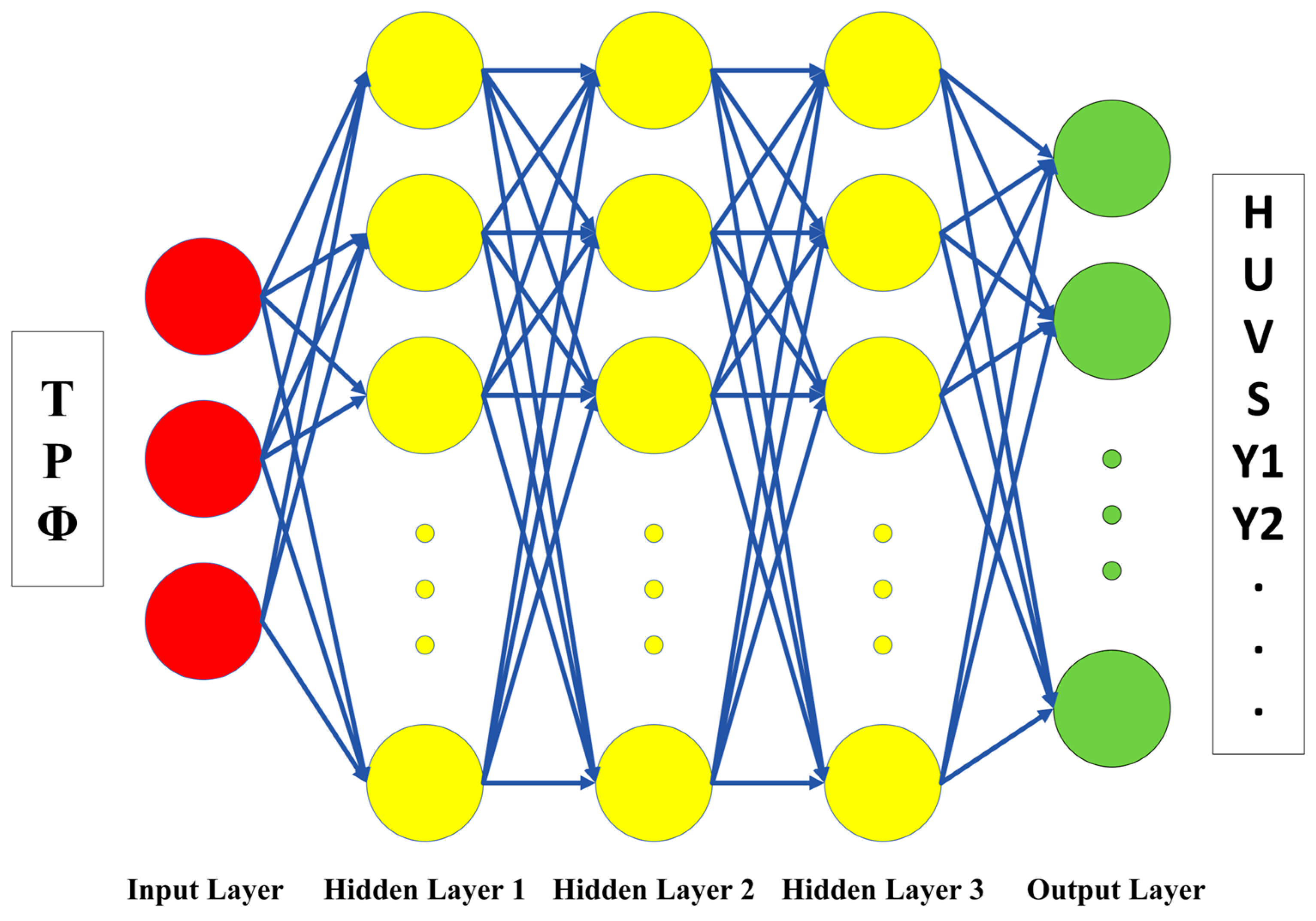
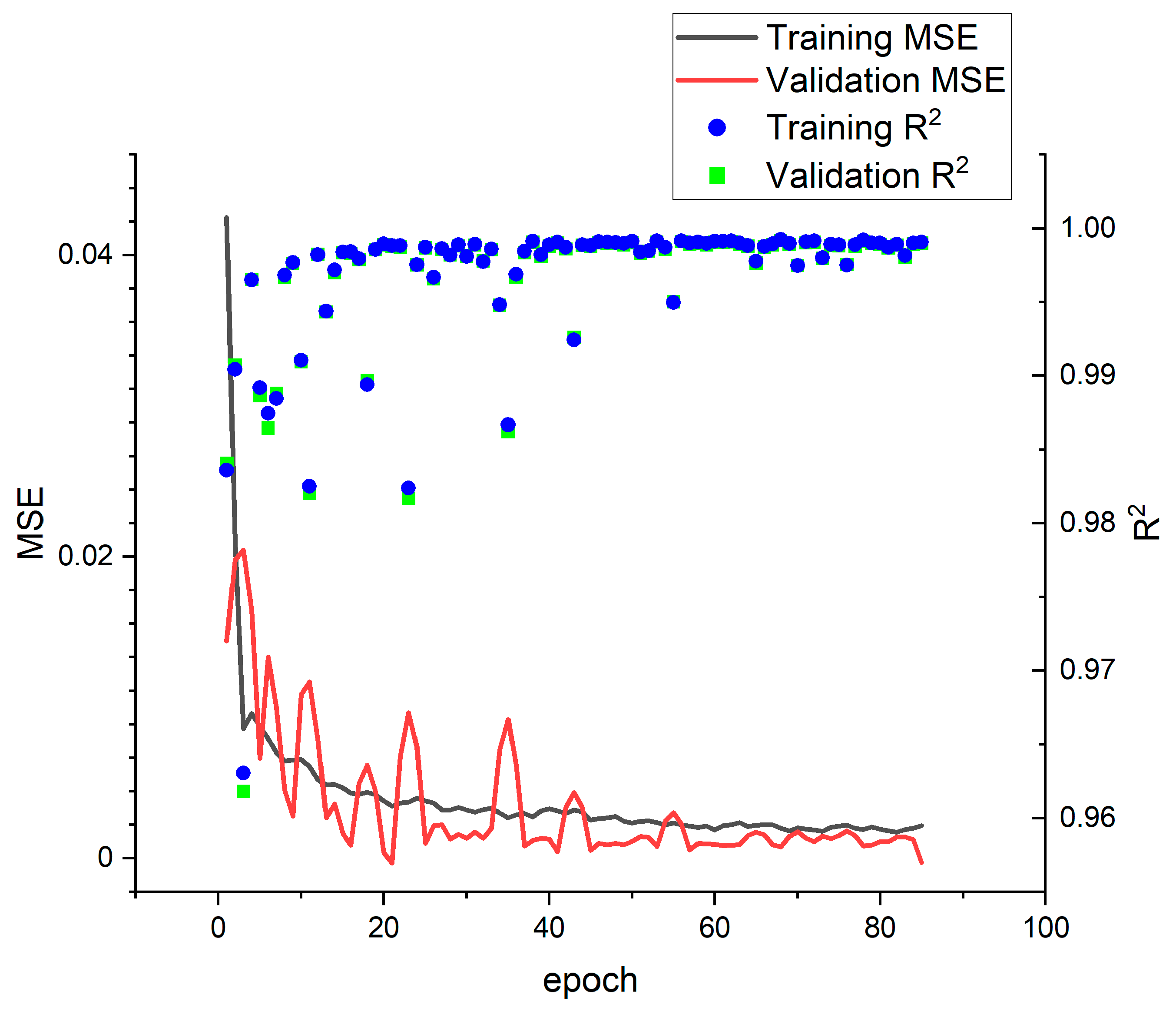
The performance of the developed deep neural network was first examined with respect to its training behavior and its ability to reproduce equilibrium thermodynamic properties and species mole fractions across the full range of pressure, temperature, and equivalence ratio conditions. Results are illustrated in Figure 2. The evolution of the training and validation losses, together with the corresponding coefficient of determination (R²), provides a clear assessment of model convergence and stability. As shown in the learning-curve plot, both the training and validation mean-squared error decrease sharply during the initial stages of optimization (before epoch 10), followed by a gradual transition toward a low-loss plateau. The validation curve shows no divergence or oscillation, indicating that there is no overfitting within the applied early-stopping window. The accompanying R² traces further suggest that the model rapidly acquires predictive capability: after only a few epochs, both the training and validation R² values exceed 0.96 and remain consistently high as the loss converges. This combined trend of synchronized MSE decay and sustained R² stability demonstrates that the selected architecture, regularization, and training configuration provide a well-posed approximation to the equilibrium mapping.

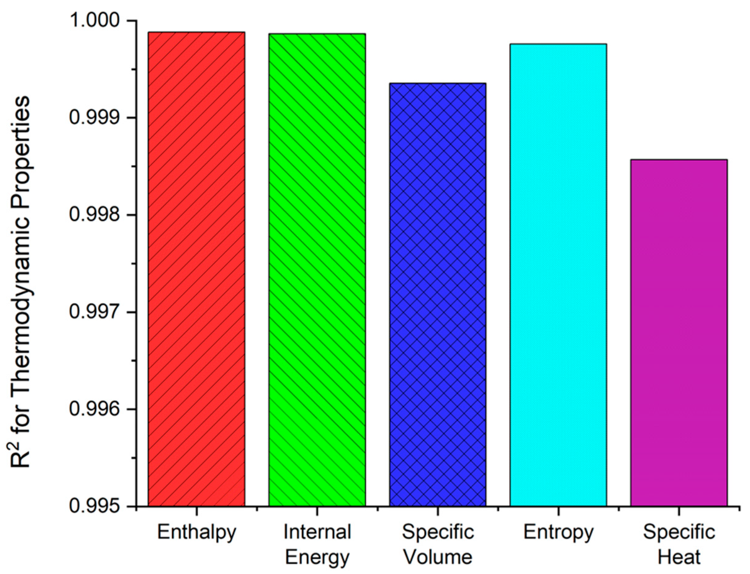
The R² scores for prediction results for five significant thermodynamic properties are shown in Figure 3. When evaluating the model on unseen validation data, the R² values for enthalpy, internal energy, specific volume, and entropy exceed 0.998, demonstrating that the network captures the underlying thermochemical structure of the equilibrium manifold with very high fidelity. Enthalpy and internal energy show the highest R² values, which indicates that the DNN model successfully captures the strong correlations with temperature and pressure. Specific heat, while accurately predicted, exhibits a slightly lower R² than the other thermodynamic quantities. This is because specific heat is a derived property, making it intrinsically more challenging to approximate. Nevertheless, the high overall R² still reflects reliable performance.

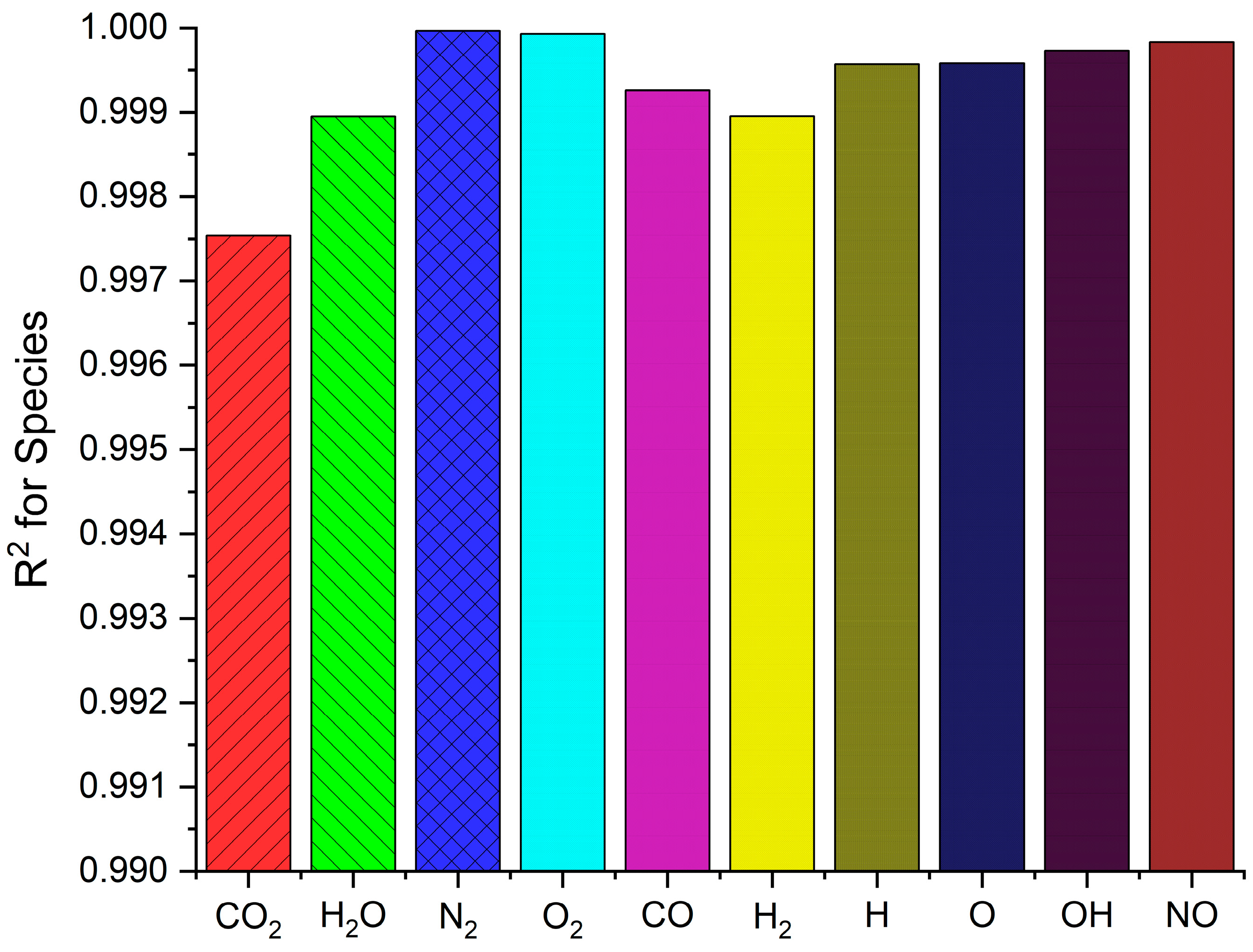
The model’s ability to predict species mole fractions is equally strong, and details are illustrated in Figure 4. All ten significant diesel products equilibrium combustion—spanning CO₂, H₂O, N₂, O₂, CO, H₂, H, O, OH, and NO—achieve R² values above 0.997. Species with monotonic variations, such as N₂ or O₂, are captured with extremely high precision, often approaching R² scores of about 0.999. CO₂ and H₂O show relatively lower R² than other species. The main reason is that CO₂ and H₂O are the dominant combustion products, and their mole fractions change sharply near stoichiometric conditions. Their profiles, therefore, show peaked, asymmetric, non-monotonic shapes. In this case, the DNN model shows slightly lower accuracy. The overall accuracy indicates that the model has learned not only the general trend of the combustion equilibrium but also its fine-scale sensitivities.

Taken together, the training–validation convergence patterns and the near-unity R² values across all outputs demonstrate that the developed neural network provides an accurate and physically consistent surrogate for the underlying equilibrium chemistry calculations. This strong baseline performance provides a foundation for subsequent uncertainty quantification and interpretability analyses, which rely on a well-trained predictor to reveal how uncertainty propagates through the model and how input conditions influence the predicted thermochemical state.

The computational efficiency of the proposed DNN surrogate model was quantitatively evaluated and compared against the equilibrium combustion solver from NASA CEA. The CEA code, originally developed by Gordon and McBride, is a well-established and extensively validated tool for computing equilibrium product compositions and thermodynamic properties in combustion and high-temperature reacting systems, and it has been widely applied in propulsion and engine-related analyses [39]. The benchmark dataset consisted of 10⁵ independent thermodynamic states uniformly sampled within the valid input domain of the DNN model, covering the same ranges of pressure, temperature, and equivalence ratio used during training.

All computations were performed on the same server platform equipped with dual-socket AMD EPYC 7R32 processors, provided by Zhejiang University—University of Illinois at Urbana-Champaign Institute, Haining, China, ensuring a fair comparison under identical hardware conditions. For the conventional equilibrium approach, the NASA CEA solver required 1.243 s to evaluate all 10⁵ states, corresponding to an average computational cost of 12.43 μs per thermodynamic state. This cost reflects the iterative nature of the equilibrium calculation, which involves nonlinear minimization of Gibbs free energy and repeated evaluation of thermodynamic property polynomials. In contrast, once trained, the DNN surrogate evaluated the same 10⁵ equilibrium states in only 0.069 s, corresponding to an average inference time of 0.691 μs per state. As a result, the DNN model achieves an approximately 18× speedup relative to the NASA CEA solver on the same CPU hardware. This performance gain arises from the fact that DNN inference consists primarily of dense matrix–vector multiplications and activation function evaluations, which scale linearly with the number of neurons and are highly optimized in modern numerical libraries.

It is important to emphasize that this comparison focuses exclusively on inference cost, which is the dominant factor in practical applications such as large-scale parametric sweeps, real-time control, uncertainty propagation, and integration into CFD or system-level simulations. Although the DNN requires an upfront training cost, this cost is incurred only once and is amortized over potentially millions of subsequent evaluations. In contrast, the equilibrium solver incurs the full iterative computational cost at every evaluation, regardless of how many states are queried.

Overall, these results demonstrate that the proposed DNN surrogate provides a substantial reduction in computational cost while maintaining high predictive accuracy, making it particularly well-suited for high-throughput equilibrium calculations, real-time applications, and data-driven combustion modeling frameworks where repeated equilibrium evaluations are required.

3.2. Uncertainty Quantification for the DNN Model

Uncertainty quantification (UQ) provides a complementary perspective to the deterministic accuracy metrics discussed previously. Whereas R² values reflect how well the model maps inputs to outputs on average, uncertainty estimates characterize the model’s confidence in each individual prediction. The present work employs Monte Carlo dropout to quantify epistemic uncertainty, in which repeated stochastic forward passes yield a distribution of predicted values for each thermochemical quantity. This approach allows the model to express its confidence in regions where training data are dense while indicating reduced reliability in sparse or highly nonlinear regions of the state space.

Table 3. Correlation coefficient and coverage behavior for outputs.

Outputs	Correlation Coefficient	Coverage Under the 2σ Uncertainty Band
Specific Heat	0.354862	0.966967
Enthalpy	0.085239	0.999837
Entropy	0.470126	0.998789
Internal Energy	0.083768	0.999755
Specific Volume	0.776795	0.978801
CO2	0.527105	0.998462
NO	0.624803	0.969611
H2O	0.577851	0.999686
N2	0.366757	0.999895
O2	0.515087	0.973688
CO	0.375612	0.99887
H2	0.527632	0.998661
H	0.554684	0.906375
O	0.732938	0.968900
OH	0.544882	0.957637

illustrates the correlation coefficients and coverage behavior for all 15 outputs. The correlation coefficient quantifies the strength of the association between the predicted epistemic variance and the true squared prediction error. A higher correlation coefficient indicates that greater predicted uncertainty is associated with higher actual error, suggesting that the model can recognize conditions in which it is less confident. To interpret correlation coefficients between predictive variance and absolute error, we adopt the following qualitative thresholds: r > 0.7 (strong), 0.3 < r ≤ 0.7 (moderate), and r ≤ 0.3 (weak). Under this criterion, most outputs exhibit strong or moderate correlation, indicating a meaningful relationship between epistemic uncertainty and prediction deviation. This suggests that Monte Carlo Dropout captures the model’s lack of knowledge in physically complex regions, leading to interpretable and well-calibrated uncertainty estimates. It should be noted that enthalpy and internal energy show weak correlation. In this case, the prediction error magnitude is uniformly small across the domain, resulting in limited dispersion in both error and predictive variance. In such near-deterministic regimes, correlation coefficients become insensitive indicators of uncertainty alignment, even though coverage remains high. The coverage value complements this interpretation. Coverage measures the fraction of samples for which the true mole fraction lies within the predicted ±2σ band. Higher coverage indicates an uncertainty estimate that neither underestimates variance nor overestimates variance. Most species achieve coverage near or above the nominal coverage expected for a Gaussian distribution of 0.95. This indicates their uncertainty bands are well calibrated: σ is neither artificially inflated nor overly narrow. Together, the correlation and coverage analyses demonstrate that the model can quantify its confidence in thermal characteristic predictions.

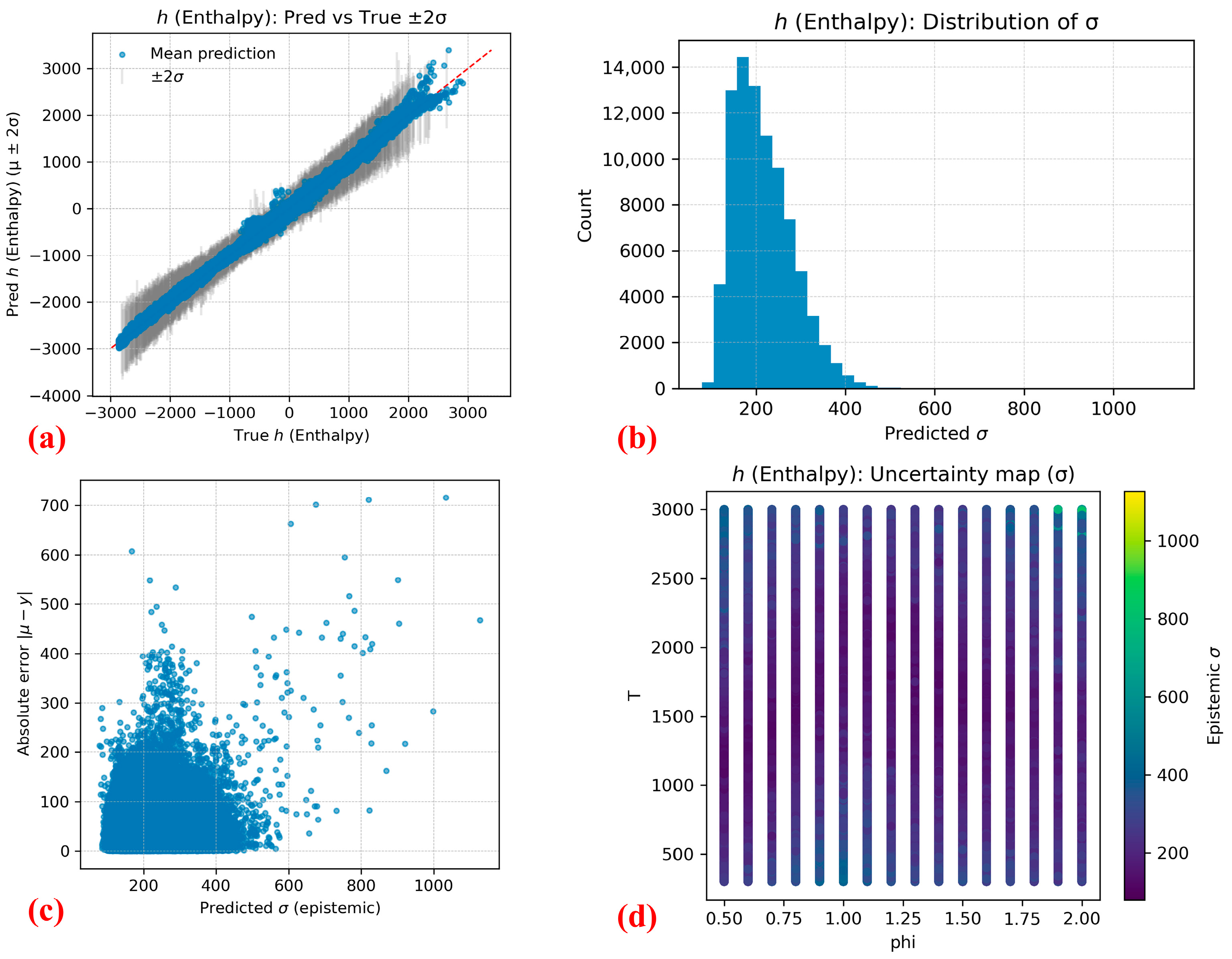
Although the neural network produces predictions for 15 thermophysical and chemical quantities, presenting full uncertainty and explainability diagnostics for each output would require an extensive number of figures. Instead, two outputs—enthalpy (H) and carbon monoxide (CO)—are chosen as representative cases because, together, they span the essential behaviors observed across the entire target set. Enthalpy is a globally smooth function of temperature, pressure, and equivalence ratio. Its equilibrium surface contains no discontinuities, and its monotonic dependence on temperature enables the neural network to achieve extremely high accuracy with minimal epistemic uncertainty [46]. As a result, H serves as a representative example of the class of thermodynamic outputs for which the mapping from inputs to outputs is well-conditioned and straightforward to learn. CO exhibits highly nonlinear equilibrium behavior, especially near fuel-rich conditions, where dissociation and recombination reactions create steep gradients and narrow peaks in the mole fraction distribution. Therefore, the behavior observed for CO provides a meaningful illustration of model performance under chemically complex conditions. By presenting H and CO together, the analysis highlights the model’s performance in straightforward and chemically complex regimes.

Figure 5a shows the prediction results and ±2σ uncertainty intervals for enthalpy, where the red, dashed diagonal line represents the ideal 1:1 correspondence, and the grey bars represent ±2σ coverage. The majority of samples lie close to the 1:1 reference line, indicating that the DNN provides accurate mean predictions over most of the thermodynamic domain. The vertical uncertainty bars remain extremely small across the most range of H, indicating that the Monte Carlo ensemble produces highly consistent predictions. At the largest true H values, a small number of points fall below the 1:1 line, indicating that the model tends to underpredict the highest-H states. This is a classic boundary behavior, because high-H cases typically correspond to extreme temperatures and equivalence ratios where thermochemical responses are most nonlinear and training coverage is often thinner.

Figure 5b shows the statistical distribution of the predicted epistemic standard deviation σ for enthalpy. The distribution of the predicted epistemic standard deviation σ remains highly concentrated near zero, suggesting that the DNN is confident for the majority of equilibrium states. Figure 5c illustrates the calibration quality of the uncertainty estimates by comparing the absolute prediction error ∣μ − y∣ against the predicted uncertainty σ. The relationship between absolute prediction error and predicted uncertainty shows a clearer positive trend, indicating that uncertainty magnitude is positively associated with actual prediction difficulty. The majority of samples with low σ exhibit correspondingly small errors, while larger errors are increasingly associated with higher predicted uncertainty.

Figure 5d visualizes the epistemic uncertainty for enthalpy across the input domain, projected onto the (T, ϕ) plane. Low uncertainty dominates most of the interior domain, consistent with the high accuracy observed in the corresponding predictions. Greater uncertainty is concentrated in regions characterized by high temperatures over 2500 K and equivalence ratios conditions over 1.75, which are closer to the boundaries of the training domain and are known to exhibit stronger nonlinearity in thermodynamic characteristics. Overall, this distribution further supports the physical plausibility of the uncertainty estimates and their consistency with model performance trends.

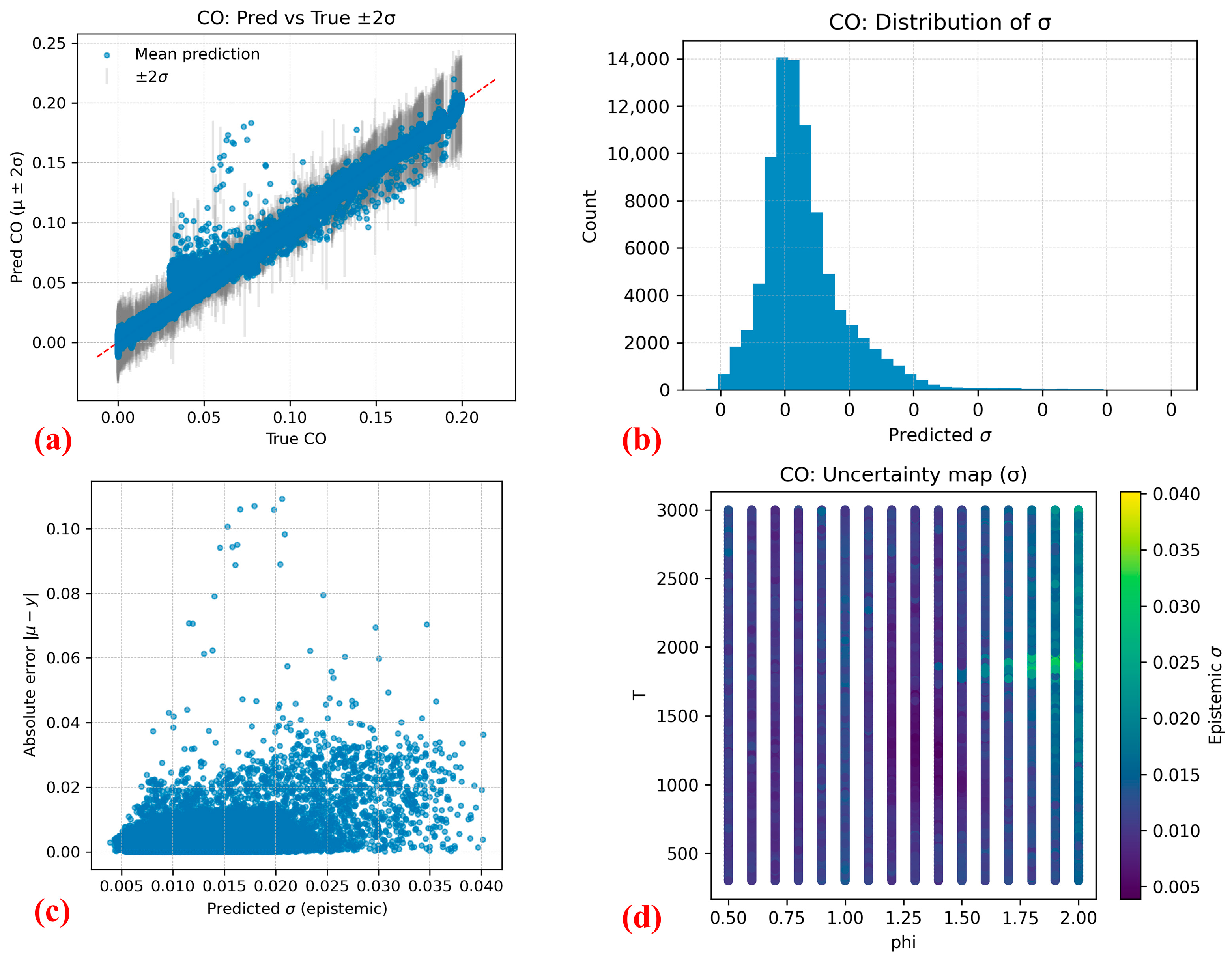
Figure 6a presents the comparison between predicted and true CO mole fractions together with the associated epistemic uncertainty bands. Overall, the predicted mean values follow the 1:1 reference line reasonably well, indicating that the DNN captures the dominant trends of CO formation under equilibrium conditions. However, compared with thermodynamic properties such as enthalpy, a noticeably larger scatter is observed. This behavior reflects the strong nonlinearity and sensitivity of CO equilibrium concentration to local temperature and equivalence ratio. Figure 6b shows the distribution of the predicted epistemic standard deviation for CO. Unlike enthalpy, the CO uncertainty distribution is broader and less sharply concentrated near zero, indicating a generally higher level of model uncertainty for this species. Overall, a large portion of samples still exhibits relatively low uncertainty. Figure 6c evaluates the calibration quality of the uncertainty estimates by plotting the absolute prediction error against the predicted σ. A clear positive trend is observed, indicating that higher predicted uncertainty generally coincides with larger prediction errors. This suggests that the uncertainty estimates for CO are informative and capture the relative difficulty of prediction. Figure 6d illustrates the distribution of epistemic uncertainty for CO across the input parameter space, projected onto the (T, ϕ) plane. Greater uncertainty is strongly localized in high-temperature and rich-mixture regions, particularly when the temperature exceeds 1500 K, and the equivalence ratio exceeds 1.5. Under these conditions, CO formation is most sensitive to changes in thermodynamic parameters, as equilibrium shifts rapidly between CO and CO₂ [47]. Overall, the spatial uncertainty distribution is physically consistent and consistent with known combustion-chemistry characteristics of CO.

3.3. Explainability Analysis

To understand how the neural network internally represents the diesel equilibrium combustion, SHAP analysis is conducted for representative thermodynamic and species outputs. SHAP plot quantifies the marginal contribution of each input variable—pressure, temperature, and equivalence ratio—to the model’s prediction at each sample point. To provide a quantitative global interpretation, the mean absolute SHAP values were computed for each feature and averaged across all outputs. The resulting global importance ranking indicates that temperature accounts for approximately 64% of the total contribution, followed by the equivalence ratio of 20% and pressure of 16%. This ranking is consistent with thermochemical principles: equilibrium composition and thermodynamic properties are primarily governed by temperature, the equivalence ratio determines the reaction stoichiometry, and pressure exerts a secondary influence. Due to space limitations, only representative SHAP plots are shown. These selected outputs were chosen to illustrate distinct physical regimes, including thermodynamic properties and radical species.

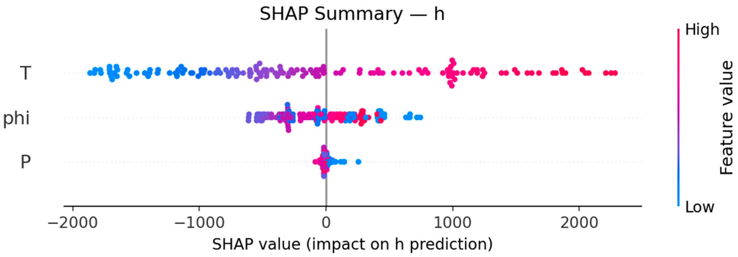
SHAP summary for enthalpy is illustrated in Figure 7. The SHAP distribution for enthalpy shows a strong, highly structured dependence on temperature. Across the entire domain, temperature exhibits SHAP amplitudes that are orders of magnitude larger than those of pressure and equivalence ratio. High-temperature samples, colored in red on the plot, consistently push enthalpy predictions toward higher values—often exceeding 2000 in SHAP magnitude—while low-temperature points contribute strongly toward lower enthalpy. This is consistent with thermodynamics: the sensible enthalpy is primarily determined by temperature in equilibrium combustion. Higher temperature increases enthalpy and shifts the equilibrium position according to Le Châtelier’s principle, thereby altering the overall enthalpy change. The SHAP distribution for the equivalence ratio is narrower but still exhibits a clear structure. Purple dots where the equivalence ratio is close to the stoichiometric ratio concentrate on the left side of the plot. These patterns are consistent with the expected thermodynamic behavior, in which maximum energy release occurs at or near the stoichiometric ratio, where combustion is most complete. Pressure contributes minimally to enthalpy predictions, with SHAP values tightly clustered around zero. This is because enthalpy in constant-pressure equilibrium calculations is mainly governed by temperature and species composition. Overall, the SHAP results suggest that the network captures physically meaningful enthalpy behavior, with temperature dominating the mapping and equivalence ratio acting as a secondary but interpretable modifier.

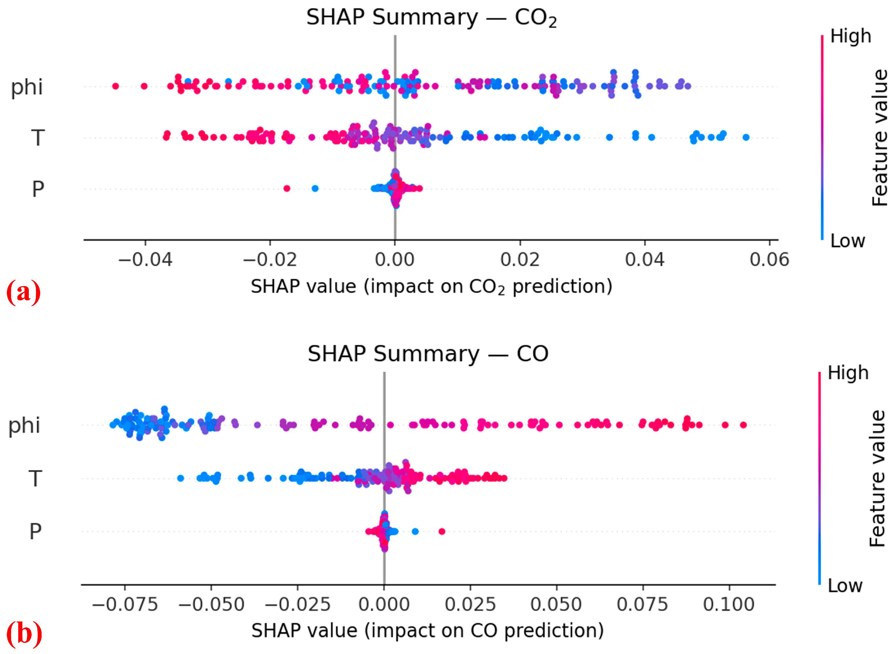
The SHAP analysis for CO₂ and CO is shown in Figure 8, which presents an interpretive picture shaped by the chemical kinetics underlying CO–CO₂ interconversion. The most influential input is the equivalence ratio. Lean mixtures produce strongly positive SHAP on CO₂ and negative SHAP contributions on CO. In contrast, fuel-rich mixtures increase CO predictions and decrease the CO₂ SHAP value. This is consistent with equilibrium chemistry: under rich conditions, oxygen is limiting, and carbon preferentially remains in partially oxidized forms, whereas under lean conditions it is largely oxidized to CO₂. Temperature also plays a substantial role, but with a more complex sign structure. Because the equilibrium constants depend exponentially on temperature via the relation K(T) = exp(−ΔG°/RT), dissociation reactions such as CO₂ ⇌ CO + 1/2O₂ exhibit strong temperature sensitivity. The enthalpy-driven increase in equilibrium constants at high temperatures promotes molecular dissociation, while entropy contributions further amplify species redistribution [37]. Therefore, the temperature-dominant behavior learned by the DNN surrogate reflects physically meaningful thermodynamic constraints rather than empirical curve fitting. At low temperatures, CO formation is suppressed, producing negative SHAP values. As the temperature increases, the SHAP values for CO become increasingly positive. This effect corresponds to the thermal decomposition of CO₂ and the contribution of high-temperature dissociation to CO formation [48]. The model, therefore, successfully captures the correct temperature dependence characteristic of high-temperature equilibrium chemistry. As with enthalpy, pressure exhibits the smallest SHAP magnitudes. Equilibrium CO₂ and CO are only weakly dependent on pressure over the typical range of combustion applications, and the network characterization reflects this physical insensitivity. Together, the SHAP results validate that the network not only predicts CO₂ and CO accurately but does so for the correct physical reasons. Fuel equivalence ratio and temperature dominate CO formation, and the learned directional contributions align with the chemical pathways that govern C–O–H equilibrium.

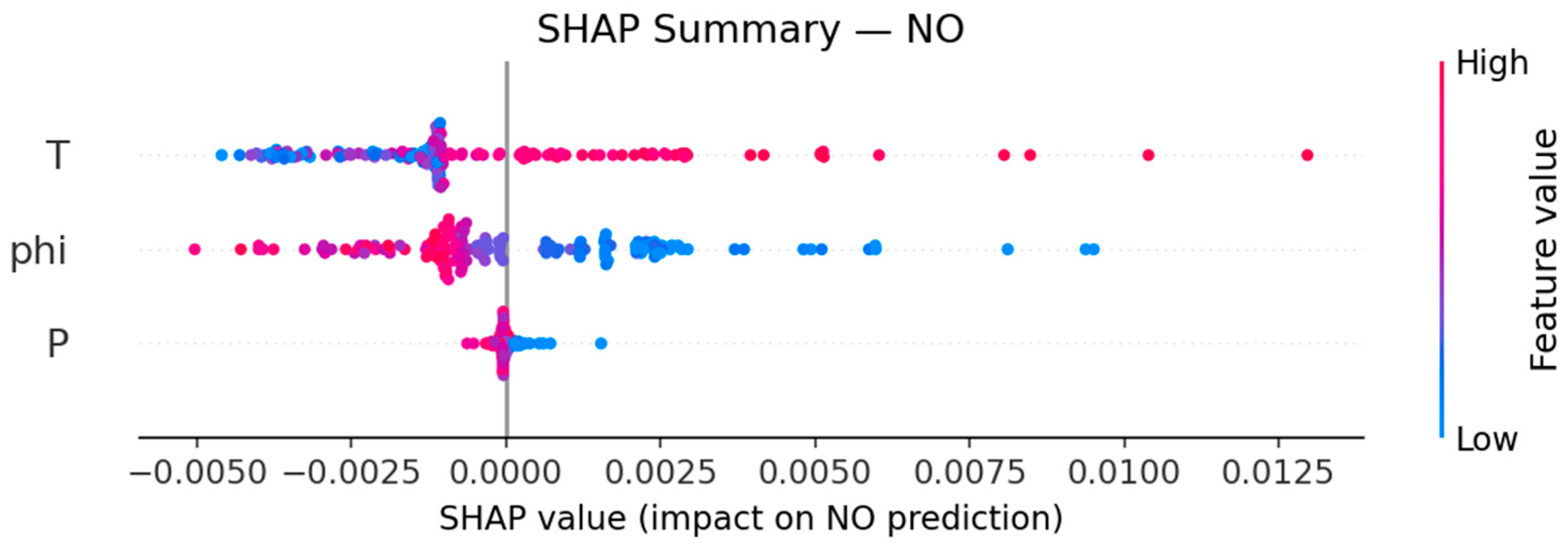
Figure 9 illustrates the SHAP results of NO. The SHAP summary plot indicates that temperature (T) is the dominant driver of NO prediction, followed by the equivalence ratio (ϕ), while pressure (P) plays a comparatively minor role. High temperature values consistently yield positive SHAP values, indicating that they increase the predicted NO concentration, while low temperatures yield negative SHAP values, indicating that they decrease the predicted NO concentration. This behavior is fully consistent with equilibrium thermal NO chemistry, in which NO formation increases rapidly with temperature due to enhanced dissociation of molecular nitrogen and oxygen [49]. The equivalence ratio also strongly influences NO prediction. Lean mixtures tend to contribute positively to NO formation, while rich mixtures are associated with negative SHAP values. This reflects the role of oxygen availability in regulating NO production: even at high temperatures, oxygen-deficient rich mixtures suppress NO formation, whereas lean conditions favor NO by providing sufficient oxidizer. In contrast, pressure has a negligible impact on NO prediction within the investigated range. The SHAP values for pressure are tightly clustered around zero, with minimal spread, indicating that pressure variations do not significantly alter the equilibrium NO concentration relative to temperature and equivalence ratio. Overall, the SHAP analysis suggests that the DNN has successfully learned a physically consistent set of controlling factors for NO under equilibrium conditions.

3.4. Limitations and Applicability

It should be noted that this DNN model is currently applicable only to equilibrium combustion conditions. The training dataset is generated under the assumption of instantaneous chemical equilibrium. Therefore, the model reproduces the equilibrium manifold rather than transient chemical kinetics. The model does not incorporate finite-rate chemical kinetics, molecular diffusion, viscosity variation, or gas–liquid mass transfer mechanisms. In practical reacting-flow systems, transport processes such as momentum diffusion, heat conduction, and species mass transfer will couple with chemical reactions to influence flame structure and flow behavior [50,51]. These transport-dominated regimes are beyond the scope of the present equilibrium model. Therefore, the proposed DNN framework is applicable to equilibrium thermodynamic estimation and parametric analysis but not to transient or transport-controlled combustion phenomena. Extending the current model to transient or kinetic regimes presents significant challenges. Detailed chemical kinetics requires large-scale and accurate datasets derived from reaction mechanisms. Also, transient combustion modeling requires time-resolved data, which increases computational cost and the complexity of training. Future work may explore integrating physics-informed neural networks or reduced-order kinetic regimes to bridge the gap between equilibrium models and fully transient combustion models. Despite these limitations, the present model remains highly suitable for applications where equilibrium assumptions are justified, such as preliminary thermodynamic analysis or combustion state initialization.

Although the present study focuses on predicting thermochemical equilibrium states rather than full engine combustion dynamics, the proposed model shows potential for integration into several practical combustion modeling workflows. In many combustion simulations, thermochemical equilibrium calculations are used as a fast thermodynamic closure to estimate product composition and thermodynamic properties. Within such frameworks, the equilibrium module operates as a device-independent component embedded in larger simulation environments. Replacing traditional iterative equilibrium solvers with the proposed DNN model can significantly reduce computational cost while maintaining high accuracy. This enables faster calculations for applications such as control-oriented engine models, multi-zone combustion simulations, and CFD tabulation frameworks, where equilibrium calculations are evaluated repeatedly.

Future research will focus on validating the proposed model within device-level combustion simulations. One potential direction is integrating the model into multi-zone diesel engine simulations, where equilibrium calculations are frequently required to estimate thermodynamic properties and species compositions during combustion. Another promising direction is coupling the surrogate model with CFD-based combustion simulations to accelerate equilibrium chemistry evaluations in reacting-flow solvers. Such integration would allow the model to be assessed under realistic engine operating conditions and to quantify the computational benefits in practical simulation environments. In addition, future studies may explore the use of experimental engine data to further evaluate the robustness and applicability of the proposed methodology.

4. Conclusions

This study developed a deep neural network model to predict equilibrium thermodynamic properties and major species compositions in diesel–air combustion across a wide range of pressure, temperature, and equivalence ratio conditions. The model achieved R² values over 0.99 for all fifteen outputs, demonstrating high accuracy and stable convergence without overfitting. Inference time was reduced by several orders of magnitude compared to conventional equilibrium solvers, demonstrating the potential for large-scale evaluations.

Uncertainty quantification was incorporated using Monte Carlo dropout to estimate epistemic uncertainty. Statistical analyses showed meaningful correlations between predicted uncertainty and true prediction error, with correlation coefficients over 0.5 for most outputs. Empirical coverage over 90% for outputs further suggested that the predicted uncertainty intervals were well calibrated in physical space, providing reliable confidence information alongside point predictions.

Model explainability was examined using SHAP analysis. The results revealed physically consistent control mechanisms, with temperature identified as the dominant driver of equilibrium behavior with a global mean SHAP value of 64%, while equivalence ratio and pressure played secondary roles within the investigated range. The directional effects learned by the network aligned with established combustion chemistry, indicating that the model’s predictions are based on meaningful thermodynamic relationships rather than spurious correlations.

It should be emphasized that the proposed model is intended to accelerate thermochemical equilibrium calculations rather than to directly simulate full combustion dynamics or transient chemical kinetics. The validation results demonstrate the DNN model’s ability to accurately reproduce equilibrium thermochemical solutions across a wide range of thermodynamic conditions. Extending the model to non-equilibrium regimes would require time-resolved kinetic datasets, higher computational cost, and enforcement of additional physical constraints. Future work will focus on extending the approach to multi-fuel systems, enhancing uncertainty calibration, and bridging equilibrium and kinetic modeling.