Risk-Aware Joint Bidding Strategy for Cascade Hydropower and Wind Power in Electricity Spot Markets Considering Vibration Zone Impacts

Abstract

To mitigate the compliance deviation risk induced by wind power output fluctuations, this paper proposes a two-stage joint bidding model for cascaded hydropower–wind systems within the electricity spot market framework from a price-taker perspective, explicitly accounting for the decision maker’s risk preferences. To capture the impacts of hydropower vibration zones on joint bidding decisions, the feasible output range of hydropower units is divided into multiple safe operating sub-intervals, and vibration zone avoidance is modeled using binary decision variables; meanwhile, penalty terms are incorporated into the objective function to suppress vibration zone crossing behaviors. From a risk-aware decision-making perspective, Conditional Value-at-Risk (CVaR) is adopted to quantify the downside tail risk of bidding revenues, and a risk factor is introduced to flexibly adjust the decision maker’s risk attitude. Finally, a case study based on a cascaded hydropower system and an associated wind farm in Southwest China is conducted to demonstrate the effectiveness of the proposed joint bidding strategy and to examine the impacts of risk preferences and vibration zone considerations on joint bidding outcomes.

1. Introduction

Under China’s “dual-carbon” strategy, renewable energy sources represented by wind and photovoltaic power have been rapidly integrated into the power system, with installed capacity and generation share continuously increasing [1], accelerating the construction of a renewable-dominated power system. By the end of 2025, China’s renewable installed capacity exceeded 1.69 billion kW, and its generation share continued to rise steadily [2]. With the deepening of electricity market-oriented reforms, renewable energy is shifting from guaranteed consumption to full participation in electricity spot markets, making generation revenue increasingly dependent on bidding strategies [3]. However, wind and photovoltaic outputs exhibit strong intermittency and randomness, rendering forecast errors unavoidable [4]. Consequently, renewable producers face imbalance assessments and revenue penalty risks [5], which undermine revenue stability and market competitiveness and hinder subsidy-free, market-oriented renewable energy development [6].

Against this background, improving the executability of awarded renewable energy quantities and enhancing revenue stability has become a key issue. Ref. [7] investigated the participation of “renewable energy plus energy storage” power stations in the day-ahead electricity market and derived optimal bidding strategies by adjusting energy storage charging and discharging schedules. Khaloie et al. studied wind–thermal multi-energy alliances participating in electricity markets and developed multi-stage coordinated bidding models by introducing energy storage [8] and photovoltaic generation [9] as extended scenarios, achieving coordinated optimization between generation revenue maximization and carbon emission objectives. However, under the constraints of the “dual-carbon” targets, thermal power units are inherently inconsistent with the low-carbon transition of energy systems due to their high carbon emission intensity [10]. Although energy storage can enhance system flexibility, its high investment and operating costs limit its ability to independently support large-scale wind power integration in the short term [11]. In contrast, cascade hydropower plants feature flexible start-up and shutdown, strong regulation capability, low operating costs, and low-carbon characteristics, and can effectively smooth renewable power fluctuations and improve bid executability through coordinated upstream–downstream operation [12]. Therefore, studying the joint bidding of cascade hydropower and wind power helps enhance renewable energy competitiveness in electricity spot markets and promotes renewable energy consumption [13].

In existing studies, numerous works have investigated the coordinated operation of hydropower and renewable energy from a power system dispatch perspective, such as developing multi-time-scale complementary dispatch frameworks for wind–photovoltaic–hydropower systems [14,15], or analyzing short-term compensation mechanisms by which hydropower mitigates wind and photovoltaic power fluctuations [16,17]. However, these studies are primarily conducted from a system dispatch standpoint and do not incorporate market-based bidding decisions, making it difficult to capture the role of market mechanisms in resource allocation.

In the field of hydro–wind joint participation in electricity spot markets, Ref. [18] proposed a day-ahead hydro–wind joint bidding model considering wind power forecast uncertainty, and analyzed the impact of prediction deviations on joint bidding revenue as well as the regulating role of hydropower; however, electricity price uncertainty was not incorporated into the bidding decision framework. Ref. [19] developed a multi-stage coordinated optimization framework integrating bidding, clearing, and dispatch for cascade hydropower–wind–photovoltaic alliances, but did not explicitly account for renewable power output uncertainty. Under a market environment where medium- and long-term contracts coexist with spot markets, ref. [20] proposed a two-stage stochastic optimization model considering wind and photovoltaic output uncertainty, in which cascade hydropower performs ex post regulation of day-ahead bidding deviations to mitigate imbalance penalties and enhance overall bidding revenue. Ref. [21] presented a nested optimization approach combining bidding decisions and self-scheduling, and incorporated future revenues beyond the forecast horizon into the day-ahead objective via a reservoir residual utility function. Ref. [22] further investigated hydro–wind joint bidding strategies for electricity spot markets under uncertainties in wind power output and electricity price, and introduced CVaR to characterize revenue risk. Beyond hydro–renewable alliances, related electricity market bidding studies have also embedded CVaR into stochastic decision-making frameworks. For example, ref. [23] proposed a CVaR-based stochastic wind–thermal coordination model to examine the trade-off between expected profit and risk in the day-ahead market, while ref. [24] incorporated an expected-profit–CVaR trade-off into an inner–outer two-layer stochastic mixed-integer bidding model for electricity retailers. In addition, Zoltowska [25] developed a mean–CVaR linear programming model for day-ahead bidding of EV fleet aggregators and explicitly integrated an aspiration/reservation-based formulation of the mean profit–risk criterion. This further demonstrates the relevance of risk-preference-aware stochastic linear programming approaches in electricity-market bidding problems. Nevertheless, in the specific context of cascade hydropower–renewable joint bidding, the joint modeling of explicit risk preferences with hydropower-specific operational couplings and safety-oriented operating constraints remains insufficiently explored. Moreover, if hydropower units operate within vibration zones for prolonged periods or frequently traverse such zones during regulation, cumulative fatigue, accelerated component wear, efficiency degradation, and unplanned outages may occur, thereby reducing unit lifetime and compromising operational safety [26]. However, most existing risk-aware bidding models still do not explicitly incorporate vibration-zone constraints and the operational risks associated with vibration-zone crossing into cascade hydropower–renewable bidding decisions, resulting in a gap between economic bidding strategies and practical safety-oriented operating requirements.

On the basis of the above studies, this paper proposes a two-stage stochastic optimization bidding model for cascade hydropower and wind power that explicitly considers the decision-maker’s risk preference, in which a set of representative scenarios is employed to characterize the uncertainties of wind power output and day-ahead electricity price forecasts. The model enforces vibration zone avoidance through hydropower operational constraints and incorporates penalty terms in the objective function to suppress vibration zone crossing behaviors; meanwhile, CVaR (Conditional Value-at-Risk) and a risk factor are introduced to measure the tail risk of the revenue distribution, thereby achieving a trade-off between expected revenue and risk control. In terms of revenue allocation, the Shapley value method is adopted to distribute joint bidding revenues, so as to enhance the rationality and stability of profit allocation. Finally, case studies are conducted to verify the effectiveness of the proposed model and to analyze the impacts of variations in the risk factor and vibration zone considerations on bidding decisions and revenue performance.

2. Theory and Methods

2.1. Research Framework

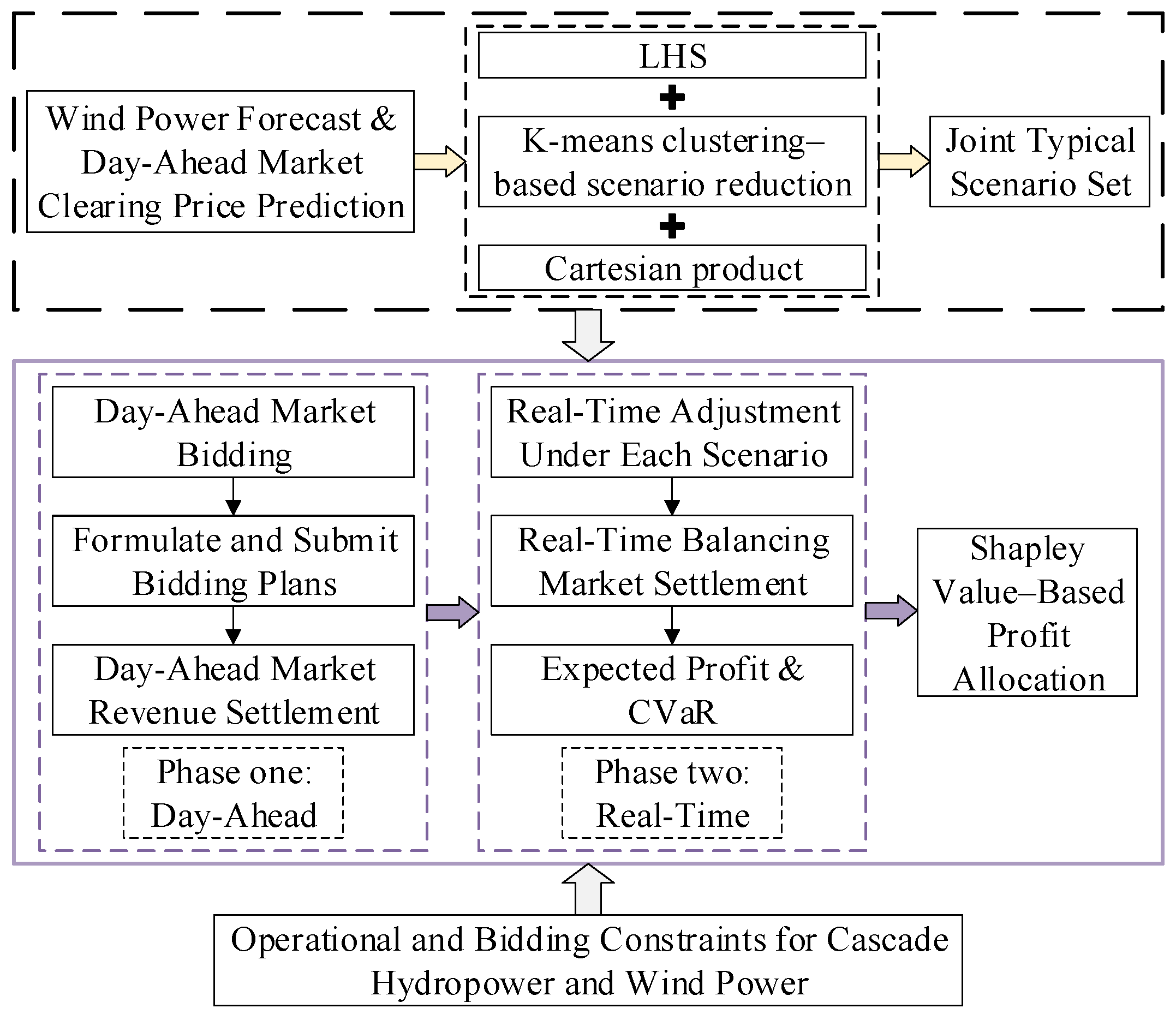
This paper develops a two-stage stochastic optimization decision-making framework for electricity spot markets, as illustrated in Figure 1. First, to capture the randomness in wind power output and electricity price forecasts, a combination of Latin Hypercube Sampling (LHS), K-means clustering-based scenario reduction, and Cartesian product construction is employed to generate a joint set of representative scenarios, preserving the statistical characteristics of both uncertainties under a controllable scenario scale. Second, within the hydropower constraints, the feasible output range of each hydropower station is divided into multiple safe operating intervals, and vibration-zone avoidance is formulated through linearization using binary (0/1) variables; meanwhile, penalty terms are incorporated into the objective function to suppress vibration-zone crossing behaviors induced by day-ahead scheduling and real-time deviation adjustments. In addition, the model accounts for dynamic water flow delay, where the inter-reservoir flow delay is modeled as a piecewise function of discharge flow and linearized via binary variables. Subsequently, Conditional Value-at-Risk (CVaR) is introduced to quantify the downside tail risk of revenue, with decision-makers’ risk preferences parameterized to enhance strategy robustness. Finally, under the market mechanism of “day-ahead bidding–real-time deviation settlement,” a CVaR-based two-stage joint bidding model is established with the objective of maximizing the expected joint bidding revenue, and its effectiveness is validated through case studies.

2.2. Representative Scenario Set

Both wind power output and day-ahead market-clearing electricity price forecasts exhibit significant uncertainty, and their fluctuation characteristics and correlations directly affect generators’ bidding strategies and revenue performance. Therefore, constructing a representative scenario set that can accurately reflect the stochastic nature of wind power and electricity price generation processes constitutes the basis of the joint bidding model.

2.2.1. Generation of Original Random Scenarios Based on LHS

In the bidding optimization problem, the forecasted wind power output and the forecasted day-ahead market-clearing electricity price are treated as two mutually independent random variables. Let $x_t^{pre}$ denote the forecast value of a random variable at time period t; then:

$$x_t=x_t^{pre}+{\epsilon }_t,{\epsilon }_t~N\left(0,{\sigma }^2\right)$$

(1)

where ${\epsilon }_t$ represents the forecast error, which is assumed to follow a normal distribution, and σ² is the variance of the normal distribution.

In this paper, the Latin Hypercube Sampling (LHS) method is adopted to construct the original scenario set. The value range [0, 1] of the cumulative distribution function (CDF) $F_t\left({\epsilon }_t\right)$ of the forecast error is evenly divided into N sub-intervals, and one sample unit is randomly drawn from each sub-interval. The error samples are then obtained through the inverse function of $F_t\left({\epsilon }_t\right)$, i.e.,

$${\epsilon }_t^{(n)}=F_t^{-1}\left(u_n\right),n=1,2,\dots ,N$$

(2)

where ${\epsilon }_t^{\left(n\right)}$ represents the n-th sampled value of the forecast error at time period t. By adding it to the original forecast value, the expression of the original random scenario samples and their matrix form can be obtained as follows:

$$\left\{\begin{array}{l}{x}_t^{(n)}=x_t^{pre}+{\epsilon }_t^{(n)}\\ X_{NT}=\left[\begin{array}{cccc}{x}_1^{(1)}& x_2^{(1)}& \dots & x_T^{(1)}\\ x_1^{(2)}& x_2^{(2)}& \dots & x_T^{(2)}\\ ⋮& ⋮& \ddots & ⋮\\ x_1^{(N)}& x_2^{(N)}& \dots & x_T^{(N)}\end{array}\right]\end{array}\right.$$

(3)

2.2.2. Representative Scenario Reduction Based on K-Means Clustering

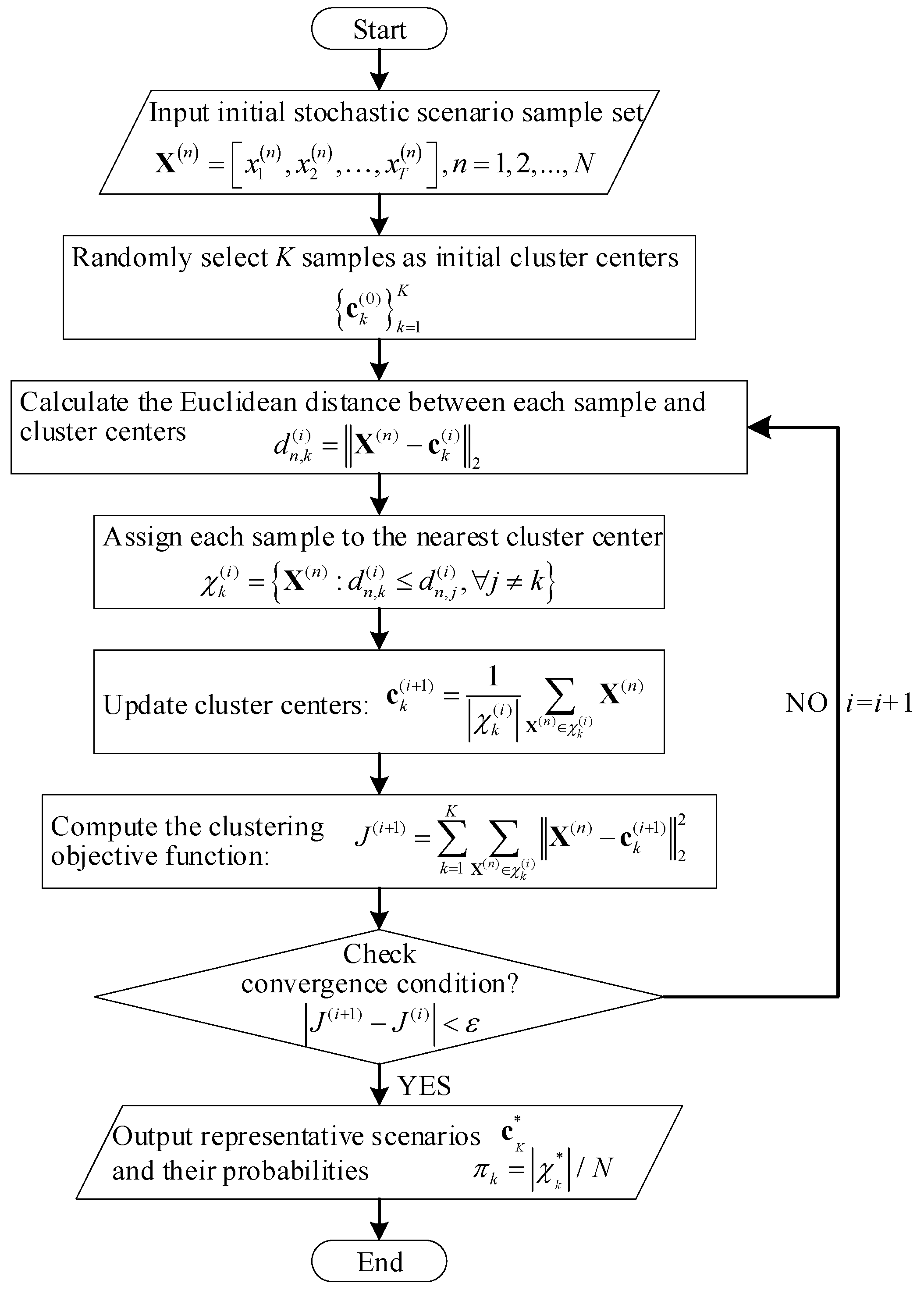
To extract representative scenarios from a large number of original random scenarios, this paper applies the K-Means clustering method to perform scenario reduction on the original scenario set generated by the LHS method, thereby obtaining a limited number of representative scenarios and calculating the occurrence probability of each representative scenario. The detailed procedure is illustrated in Figure 2. Through K-Means-based scenario reduction, the statistical characteristics of the original random scenarios are well preserved while the scenario scale is effectively reduced, which significantly improves the computational efficiency of the subsequent stochastic optimization model.

2.2.3. Cartesian Product Combination

This study adopts a Cartesian product approach to combine the representative scenario sets of day-ahead electricity prices and wind power output, thereby constructing a joint uncertainty scenario set [22]. Specifically, if the numbers of representative scenarios for wind power output and day-ahead electricity prices are S_w and S_λ, respectively, a total of S = S_w × S_λ joint scenarios are generated. Each joint scenario consists of one wind power output trajectory and one electricity price trajectory, and its probability is given by the product of the corresponding scenario probabilities.

2.3. Risk Measure: CVaR

CVaR (Conditional Value-at-Risk) is derived from VaR (Value-at-Risk) and can directly quantify extreme tail risk [27]. CVaR focuses on the expected loss exceeding the VaR threshold, which directly reflects the severity of extreme risk and exhibits higher sensitivity to tail risk. Therefore, this paper adopts CVaR as the risk measure to characterize downside revenue risk.

At a given confidence level α, the VaR of the random revenue F is defined as follows:

$$Va{R}_{\alpha }\left(F\right)=\inf \left\{\kappa \in ℝ\left|\mathbb{P}\left(F\le \kappa \right)\ge \alpha \right.\right\}$$

(4)

Since this paper focuses on “revenue” rather than “loss”, the downside tail of the revenue distribution is measured; when the revenue falls below a given quantile, a higher average value of the lower-tail revenue indicates a more robust decision. On this basis, CVaR can be interpreted as the expected value of the worst (1 − α) portion of the revenue distribution. For the revenue F, the CVaR at confidence level α is defined as follows:

$$CVa{R}_{\alpha }\left(F\right)=\mathbb{E}\left[F\left|F\le Va{R}_{\alpha }\left(F\right)\right.\right]$$

(5)

CVaR can be equivalently expressed in the following optimization form:

$$CVa{R}_{\alpha }\left(F\right)=\underset{\kappa \in ℝ}{\max }\left\{\kappa -{\displaystyle \frac{1}{1-\alpha }}\left[{\left(\kappa -F\right)}^{+}\right]\right\}$$

(6)

In the case of discrete scenarios:

$$CVa{R}_{\alpha }\left(F\right)=\underset{\kappa ,{\zeta }_s}{\max }\left\{\kappa -{\displaystyle \frac{1}{1-\alpha }}{\displaystyle \sum _{s=1}^S{\pi }_s{\zeta }_s}|{\zeta }_s\ge \kappa -F_s,{\zeta }_s\ge 0\right\}$$

(7)

where κ is an auxiliary variable for CVaR calculation, S is the scenario set, π_s represents the probability of scenario s, and ζ_s is an auxiliary variable associated with scenario s.

2.4. Vibration Zones and Water Flow Delay

2.4.1. Definition of Vibration Zone Crossing and Vibration Zone Avoidance

In this paper, vibration zone avoidance refers to the operational requirement that hydropower units should avoid operating within vibration zones and remain within predefined safe operating zones as much as possible. In contrast, vibration zone crossing refers to the behavior in which hydropower output passes across vibration-zone intervals during output variations. It can be specifically classified into day-ahead-stage vibration zone crossing and real-time adjustment-stage vibration zone crossing. The day-ahead-stage vibration zone crossing refers to the vibration-zone intervals crossed by the hydropower bidding output between adjacent time periods during the day-ahead bidding stage; the real-time adjustment-stage vibration zone crossing refers to the vibration-zone intervals crossed along the adjustment path of real-time output relative to the day-ahead bidding output when hydropower plants adjust their output in real-time operation to eliminate deviations. Although neither type of crossing behavior results in the hydropower output finally operating within vibration zones, such transition processes may still induce potential risks in practical engineering operation and therefore need to be suppressed.

For a given hydropower plant, suppose it has VN vibration zones; then there are SN = VN + 1 safe output zones.

The schematic diagram of vibration zones is shown in Figure 3.

In the figure, $p_k^{vib - lb}$ and $p_k^{vib - ub}$ represent the lower bound and upper bound of the k-th vibration zone, respectively. Accordingly, the lower and upper bounds of each safe zone are given as follows:

$$\left\{\begin{array}{l}\begin{array}{cc}\begin{array}{cc}{p}_1^{safe-lb}=p^{\min },& p_1^{safe-ub}=p_1^{vib-lb}\end{array}& (k=1)\end{array}\\ \begin{array}{cc}\begin{array}{cc}{p}_k^{safe-lb}=p_{k-1}^{vib-ub},& p_k^{safe-ub}=p_k^{vib-lb}\end{array}& (1<k<SN)\end{array}\\ \begin{array}{cc}\begin{array}{cc}{p}_{SN}^{safe-lb}=p_{SN-1}^{vib-ub},& p_{SN}^{safe-ub}=p^{\max }\end{array}& (k=SN)\end{array}\end{array}\right.$$

(8)

By introducing a binary variable $y_k^h$, which represents whether the hydropower output lies in the k-th safe zone (1 for yes, 0 for no), vibration zone avoidance can be linearly modeled as follows [28]:

$$\left\{\begin{array}{l}{\displaystyle \sum _{k=1}^{SN}{p}_k^{safe-lb}\cdot y_k^h}\le p\le {\displaystyle \sum _{k=1}^{SN}{p}_k^{safe-ub}\cdot y_k^h}\\ {\displaystyle \sum _{k=1}^{SN}{y}_k^h=1}\end{array}\right.$$

(9)

In addition, the expression ${\sum }_{k=1}^{SN}k\times y_k^h$ represents the index of the safe zone in which the hydropower output is located.

2.4.2. Dynamic Water Flow Delay

Existing studies [19] mostly consider the water flow delay between cascade hydropower plants as a fixed constant, whereas this paper investigates dynamic water flow delay, that is, the water flow delay is a piecewise function of the discharge flow, as shown below.

$$\tau =\left\{\begin{array}{cc}{\tau }_1& 0\le Q^{out}<q{U}_1\\ {\tau }_2& q{L}_2\le Q^{out}<q{U}_2\\ \dots & \dots \\ {\tau }_n& q{L}_n\le Q^{out}<q{U}_n\\ \dots & \dots \\ {\tau }_N& q{L}_N\le Q^{out}<q{U}_N\end{array}\right.$$

(10)

where Q^out represents the discharge flow of the hydropower plant. The water flow delay is divided into N segments; τ_n represents the water flow delay in the n-th segment, and qL_n and qU_n represent the lower and upper bounds of the discharge flow corresponding to the n-th segment, respectively. By introducing binary variables, the above piecewise relationship can be linearized as follows:

$$Q^{out}={\displaystyle \sum _{n=1}^N{q}_n^{out}}$$

(11)

$$q{L}_n\cdot y_n^w\le q_n^{out}\le q{U}_n\cdot y_n^w$$

(12)

$${\displaystyle \sum _{n=1}^N{y}_n^w}=1$$

(13)

where $y_n^w$ is a binary variable representing whether the discharge flow lies in the n-th segment, and $q_n^{out}$ represents the component of the discharge flow in the n-th segment.

2.5. CVaR-Based Two-Stage Bidding Model

The proposed model assumes that the alliance acts as a price taker; therefore, in the day-ahead stage, it only decides the submitted energy quantities and does not participate in price bidding.

2.5.1. Objective Function

$$\max \left\{F^{total}-M\cdot {\displaystyle \sum _{j\in J}{\displaystyle \sum _{t=2}^{T}v{n}_{j,t}^{DA}}}-M\cdot {\displaystyle \sum _{s\in S}{\pi }_s\cdot {\displaystyle \sum _{j\in J}{\displaystyle \sum _{t=1}^{T}d{n}_{s,j,t}^{im}}}}\right\}$$

(14)

$$F^{total}=\left(1-\beta \right)\cdot {\displaystyle \sum _{s=1}^S{\pi }_s\cdot F_s}+\beta \cdot F^{CVaR}$$

(15)

$$F_s=F_s^{DA}+F_s^{im}$$

(16)

$$F^{CVaR}=\kappa -{\displaystyle \frac{1}{1-\alpha }}\cdot {\displaystyle \sum _{s=1}^S{\pi }_s\cdot {\zeta }_s}$$

(17)

$$\left\{\begin{array}{l}{\zeta }_s\ge \kappa -F_s\\ {\zeta }_s\ge 0\end{array}\right.$$

(18)

In the objective, F^total represents the total revenue, and F_s denotes the bidding revenue under scenario s. F^DA represents the revenue from the day-ahead market, while F^im represents the imbalance settlement penalty in the real-time market. S is the representative scenario set, and π_s represents the probability of scenario s. The parameter β reflects the decision-maker’s risk preference. ζ_s is an auxiliary variable used to calculate CVaR. ${vn}_{j,t}^{DA}$ represents the number of vibration zone crossings of the bidding output of hydropower plant j at time period t relative to time period t − 1 in the day-ahead stage, and ${dn}_{s,j,t}^{im}$ represents the number of vibration zone crossings of hydropower plant j at time period t during deviation adjustment under scenario s in the real-time stage. M is the monetized penalty coefficient associated with vibration-zone crossing and is set to 1000 in this study. Considering that the revenue magnitude is generally much higher, this setting allows vibration-zone-crossing behavior to be penalized without dominating the main revenue-driven bidding decision.

In Equation (15), β ∈ [0, 1] is a dimensionless parameter representing the decision-maker’s risk preference. β = 0 corresponds to the risk-neutral case, while larger β values lead to more conservative bidding decisions. Since the expected revenue term and the CVaR term are both measured in monetary units, β is used here to parameterize the trade-off between revenue pursuit and downside-risk control under different risk preferences.

Similar revenue–risk formulations combining expected profit and CVaR have been widely adopted in electricity market bidding studies [23,24,25]. In particular, Zoltowska [25] developed a mean–CVaR linear programming model for day-ahead bidding of EV fleet aggregators and explicitly incorporated an aspiration/reservation-based formulation of the mean profit–risk criterion. Following this line of research, the present study further incorporates cascade-hydropower operational couplings and vibration-zone-related operating requirements into the joint bidding framework.

(1)

Day-ahead bidding revenue.

$$F_s^{DA}={\displaystyle \sum _{t=1}^T{\lambda }_{s,t}\cdot \left({\displaystyle \sum _{j\in J}{p}_{j,t}^{hyd}}+p_t^w\right)\cdot \Delta t}$$

(19)

where λs,t represents the forecasted day-ahead electricity price at time period t under scenario s; $p_{j,t}^{hyd}$ represents the bidding output of hydropower plant j at time period t; $p_t^w$ represents the bidding output of the wind farm at time period t; Δt is the length of the time interval; J represents the set of hydropower plants; and T represents the set of time periods.

(2)

Real-time imbalance penalty.

$$F_s^{im}={\displaystyle \sum _{t=1}^T\left({\mu }^{up}\cdot {\lambda }_{s,t}\cdot P_{s,t}^{agg,dev+}-{\mu }^{down}\cdot {\lambda }_{s,t}\cdot P_{s,t}^{agg,dev-}\right)}$$

(20)

$$P_{s,t}^{agg,dev}=p_{s,t}^{w,act}+{\displaystyle \sum _{j\in J}{p}_{s,j,t}^{hyd,act}}-p_t^w-{\displaystyle \sum _{j\in J}{p}_{j,t}^{hyd}}$$

(21)

$$P_{s,t}^{agg,dev+}=\max \left(P_{s,t}^{agg,dev},0\right)$$

(22)

$$P_{s,t}^{agg,dev-}=\max \left(-P_{s,t}^{agg,dev},0\right)$$

(23)

where $P_{s,t}^{agg,dev+}$ and $P_{s,t}^{agg,dev-}$ represent the positive and negative imbalance power of the aggregated system at time period t under scenario s, respectively; $P_{s,t}^{w,act}$ and $P_{s,t}^{hyd,act}$ represent the actual outputs of the wind farm and hydropower plant j at time period t under scenario s, respectively; μ^up and μ^down are the penalty coefficients for positive and negative imbalance energy, respectively.

(3)

Vibration zone crossing.

$$v{n}_{j,t}^{DA}=\left|{\displaystyle \sum _{k=1}^{S{N}_j}k\cdot y_{j,t,k}^h}-{\displaystyle \sum _{k=1}^{S{N}_j}k\cdot y_{j,t-1,k}^h}\right|$$

(24)

$$d{n}_{s,j,t}^{im}=\left|{\displaystyle \sum _{k=1}^{S{N}_j}k\cdot y_{s,j,t,k}^{h,act}}-{\displaystyle \sum _{k=1}^{S{N}_j}k\cdot y_{j,t,k}^h}\right|$$

(25)

where SN_j represents the number of safe zones of hydropower plant j; $y_{j,t,k}^h$ is a binary indicator variable that represents whether the bidding output of hydropower plant j at time period t lies in the k-th safe zone; $y_{s,j,t,k}^{h,act}$ is a binary indicator variable that represents whether the actual output of hydropower plant j at time period t under scenario s lies in the k-th safe zone.

2.5.2. Constraints

(1)

Hydropower output limits and ramping constraints.

$$p_j^{hyd,\min }\le p_{j,t}^{hyd}\le p_j^{hyd,\max }$$

(26)

$$-Ram{p}_j^{hyd}\le p_{j,t}^{hyd}-p_{j,t-1}^{hyd}\le Ram{p}_j^{hyd}$$

(27)

where $p_j^{hyd,max}$ and $p_j^{hyd,min}$ represent the upper and lower limits of the output of hydropower plant j, respectively; ${Ramp}_j^{hyd}$ represents the ramping limit of hydropower plant j.

(2)

Vibration zone avoidance constraints.

$${\displaystyle \sum _{k=1}^{S{N}_j}{y}_{j,t,k}^h}=1$$

(28)

$${\displaystyle \sum _{k=1}^{S{N}_j}{y}_{j,t,k}^h\cdot p_{j,k}^{safe,lower}}\le p_{j,t}^{hyd}\le {\displaystyle \sum _{k=1}^{S{N}_j}{y}_{j,t,k}^h\cdot p_{j,k}^{safe,upper}}$$

(29)

where $p_{j,k}^{safe,upper}$ and $p_{j,k}^{safe,lower}$ represent the upper and lower bounds of the k-th safe output zone of hydropower plant j, respectively.

(3)

Reservoir water balance constraints.

$$Q_{j,t}^{out}={\displaystyle \sum _{n=1}^{Q{N}_j}{q}_{j,t,n}^{out}}$$

(30)

$$q{L}_{j,n}\cdot y_{j,t,n}^w\le q_{j,t,n}^{out}\le q{U}_{j,n}\cdot y_{j,t,n}^w$$

(31)

$${\displaystyle \sum _{n=1}^{Q{N}_j}{y}_{j,t,n}^w}=1$$

(32)

$$Q_{j,t}^{in}={\displaystyle \sum _{m\in HydU{p}_j}{\displaystyle \sum _{n=1}^{Q{N}_m}{q}_{m,t-{\tau }_{j,n},t}^{out}}}+Q_{j,t}^{qu}$$

(33)

$$Q_{j,t}^{gen}=p_{j,t}^{hyd}\cdot wc{r}_j\times {\displaystyle \frac{1000}{3600}}$$

(34)

$$Q_{j,t}^{out}=Q_{j,t}^{gen}+Q_{j,t}^{spill}$$

(35)

$$\left\{\begin{array}{l}\begin{array}{cc}{V}_{j,t}=V_j^{init}+\left(Q_{j,t}^{in}-Q_{j,t}^{out}\right)\cdot \Delta t\cdot 0.36& t=1\end{array}\\ \begin{array}{cc}{V}_{j,t}=V_{j,t-1}+\left(Q_{j,t}^{in}-Q_{j,t}^{out}\right)\cdot \Delta t\cdot 0.36& t>=2\end{array}\end{array}\right.$$

(36)

where QN_j represents the number of discharge flow segments of hydropower plant j; $Q_{j,t}^{in}$, $Q_{j,t}^{out}$, $Q_{j,t}^{gen}$, $Q_{j,t}^{spill}$ and $Q_{j,t}^{qu}$ represent the inflow, discharge flow, generation flow, spillage flow, and interval inflow (natural inflow) of hydropower plant j at time period t, respectively, with units of m³/s; wcr_j represents the average water consumption rate of hydropower plant j, with units of m³/kWh; V_j,t represents the reservoir storage of hydropower plant j at the end of time period t, with units of 10⁴ m³; and $V_j^{init}$ represents the initial reservoir storage of hydropower plant j.

(4)

Flow boundary constraints.

$$Q_j^{out,\min }\le Q_{j,t}^{out}\le Q_j^{out,\max }$$

(37)

where $Q_j^{out,max}$ and $Q_j^{out,min}$ represent the upper and lower limits of the discharge flow of hydropower plant j, respectively.

(5)

Water level boundary constraints.

$$H_j^{\min }\le H_{j,t}\le H_j^{\max }$$

(38)

$$H_j^{final,\min }\le H_{j,T}\le H_j^{final,\max }$$

(39)

where H_j,t represents the water level of hydropower plant j at the end of time period t, with units of m; $H_j^{max}$ and $H_j^{min}$ represent the upper and lower limits of the water level of hydropower plant j, respectively; and $H_j^{final,max}$ and $H_j^{final,min}$ represent the upper and lower limits of the final water level of hydropower plant j, respectively.

(6)

Water level–reservoir storage curve.

$$V_{j,t}=f_j^{HV}\left(H_{j,t}\right)$$

(40)

where $f_j^{HV}\left(·\right)$ represents the water level–storage curve of hydropower plant j.

(7)

Wind power constraints.

$$0\le p_t^w\le p^{w,\max }$$

(41)

where $p^{w,max}$ represents the installed capacity of wind power.

In the real-time adjustment stage, under each scenario, cascade hydropower plants are subject to constraints given in Equations (26)–(40), which are not repeated here for brevity.

3. Model Solution Strategy

The model solved in this study is the CVaR-based two-stage joint bidding model composed of the objective function in Section 2.5.1 and the operational constraints in Section 2.5.2. In this model, the vibration zone avoidance constraints and the dynamic water flow delay constraints have already been linearized in Section 2.4 by introducing binary variables. Accordingly, this section further reformulates the remaining nonlinear parts, namely, the water-level boundary constraints associated with the water level–reservoir storage curve, the positive and negative deviation power expressions in the real-time stage, and the vibration-zone-crossing terms in the objective function, so that the overall model can be transformed into a mixed-integer linear programming model (MILP).

(1)

Linearization of water level–storage curve constraints.

To avoid introducing an excessive number of binary variables, the upper and lower bounds of water level and final water level are converted into the corresponding upper and lower bounds of reservoir storage through the water level–storage curve. Therefore, the constraints on the water level and terminal water level, namely Equations (38)–(40) in Section 2.5.2, are ultimately transformed into constraints on reservoir storage and terminal reservoir storage, as follows:

$$V_j^{\min }\le V_{j,t}\le V_j^{\max }$$

(42)

$$V_j^{final,\min }\le V_{j,T}\le V_j^{final,\max }$$

(43)

(2)

Linearization of deviation power.

For the real-time imbalance settlement term in Part (2) of Section 2.5.1, the linearized expressions of the positive and negative deviation power defined in Equations (22) and (23) are given as follows:

$$P_{s,t}^{agg,dev+}-P_{s,t}^{agg,dev-}=P_{s,t}^{agg,dev}$$

(44)

$$P_{s,t}^{agg,dev+}\ge 0$$

(45)

$$P_{s,t}^{agg,dev-}\ge 0$$

(46)

(3)

Linearization of vibration zone crossing–related constraints.

For the vibration-zone-crossing penalty term in Part (3) of Section 2.5.1, the linearized forms of Equations (24) and (25) are given as follows:

$$\left\{\begin{array}{l}v{n}_{j,t}^{DA}\ge {\displaystyle \sum _{k=1}^{S{N}_j}k\cdot y_{j,t,k}^h}-{\displaystyle \sum _{k=1}^{S{N}_j}k\cdot y_{j,t-1,k}^h}\\ v{n}_{j,t}^{DA}\ge {\displaystyle \sum _{k=1}^{S{N}_j}k\cdot y_{j,t-1,k}^h}-{\displaystyle \sum _{k=1}^{S{N}_j}k\cdot y_{j,t,k}^h}\end{array}\right.$$

(47)

$$\left\{\begin{array}{l}d{n}_{s,j,t}^{im}\ge {\displaystyle \sum _{k=1}^{S{N}_j}k\cdot y_{s,j,t,k}^{h,act}}-{\displaystyle \sum _{k=1}^{S{N}_j}k\cdot y_{j,t,k}^h}\\ d{n}_{s,j,t}^{im}\ge {\displaystyle \sum _{k=1}^{S{N}_j}k\cdot y_{j,t,k}^h}-{\displaystyle \sum _{k=1}^{S{N}_j}k\cdot y_{s,j,t,k}^{h,act}}\end{array}\right.$$

(48)

4. Results and Discussion

This study takes a cascade of hydropower stations and a wind farm located in a river basin in Southwest China as the research object to validate the proposed method through a case study. The wind power forecast series is obtained from actual operational data, while the day-ahead electricity price forecast series is set with reference to typical value ranges of the Nordic electricity market, serving only to characterize price volatility rather than to represent any specific market-clearing mechanism. The case study is conducted over a 24 h scheduling horizon with a time resolution of 1 h. The model is implemented on the Python 3.12 platform and solved using the commercial optimization solver Gurobi, with experiments carried out on a system equipped with an Intel(R) Core (TM) i7-14700 processor operating at 2.5 GHz, 32 GB of RAM, and the Windows 11 operating system.

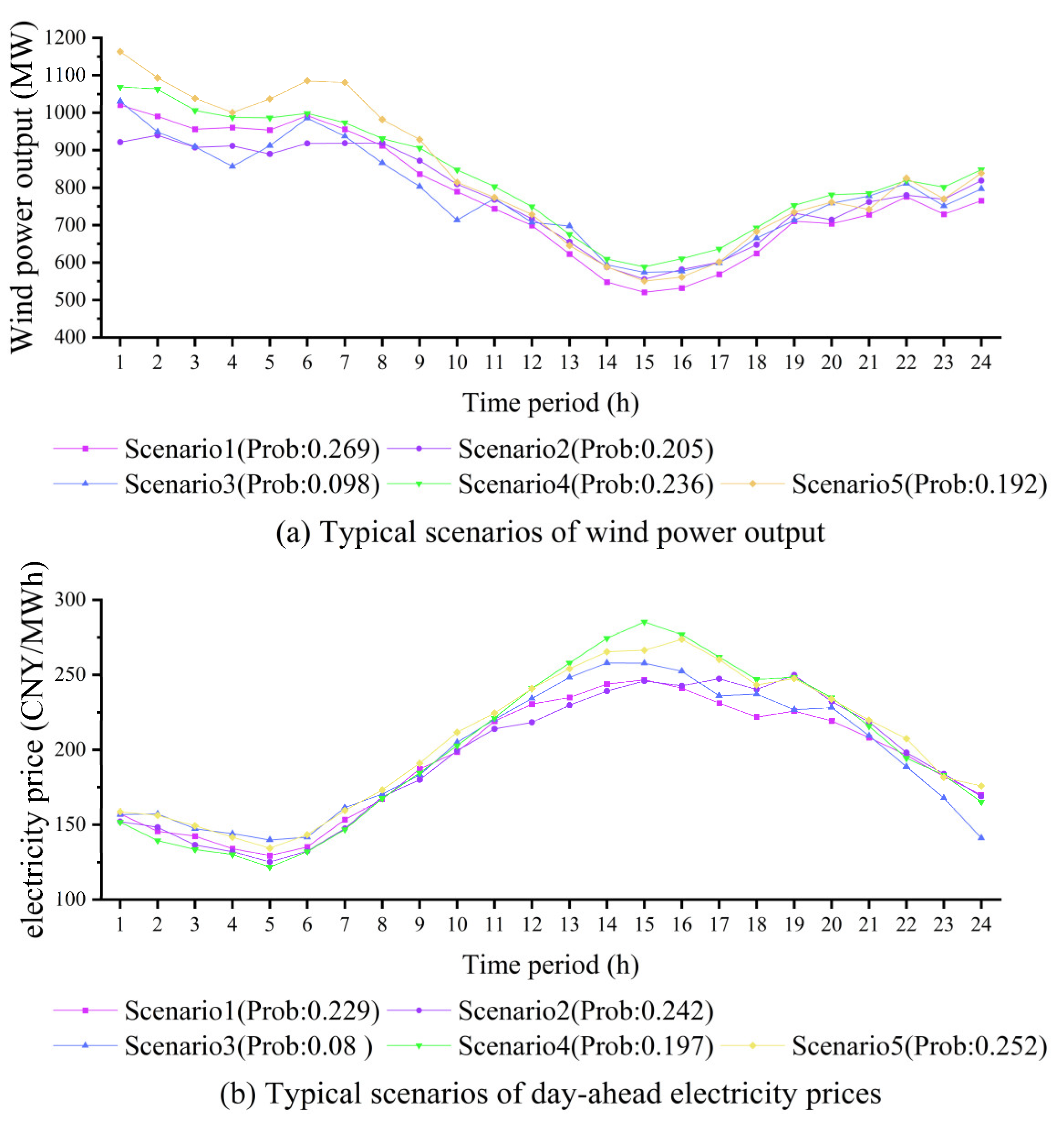
The installed capacity of the wind farm is 1200 MW. The confidence level of CVaR is set to α = 0.95. The characteristic parameters of the hydropower plants are presented in

Table 1. Main characteristic parameters of hydropower plants.

Hydropower Plant	Installed Capacity (MW)	Max Outflow (m3/s)	Water Level (m)		Initial Water Level (m)		Lower Limit of Final Water Level (m)		Average Interval Inflow (m3/s)
			Max	Min	Dry	Abundant	Dry	Abundant	Dry	Abundant
A	900	1890	1307	1303	1305.26	1306.35	1305.10	1306.15	96	332
B	4200	2103	1240.0	990.22	1139.50	1135.40	1139.35	1135.20	28	59
C	1760	2230	994	987.74	992.79	993.25	992.65	993.05	43	69

,

Table 2. Water flow delay data of hydropower plants.

Hydropower Plant	Flow Interval 1 (m3/s)	Delay Time (h)	Flow Interval 2 (m3/s)	Delay Time (h)	Flow Interval 3 (m3/s)	Delay Time (h)	Flow Interval 4 (m3/s)	Delay Time (h)
A to B	[0, 500)	8	[500, 1000)	7	[1000, 2000)	6	[2000, 3000)	5
B to C	[0, 1000)	3	[1000, 2000)	2	[2000, 3000)	1

and

Table 3. Vibration zone data of hydropower plants.

Hydropower Plant	Vibration Zone 1 (MW)	Vibration Zone 2 (MW)
A	(120, 140)
B	(0, 120)	(210, 240)
C	(0, 90)	(120, 140)

. The penalty coefficients for positive and negative imbalance energy are set to 0.4 and 1.6, respectively. In this study, the forecast errors of wind power output and day-ahead electricity prices are assumed to follow a normal distribution [29], with a standard deviation of 20%. The number of representative scenarios for each random variable is set to 5, and a total of 25 scenarios are generated through the Cartesian product combination. The generated representative scenarios are illustrated in Figure 4.

4.1. Joint Bidding Analysis

4.1.1. Analysis of the Joint Bidding Output Process

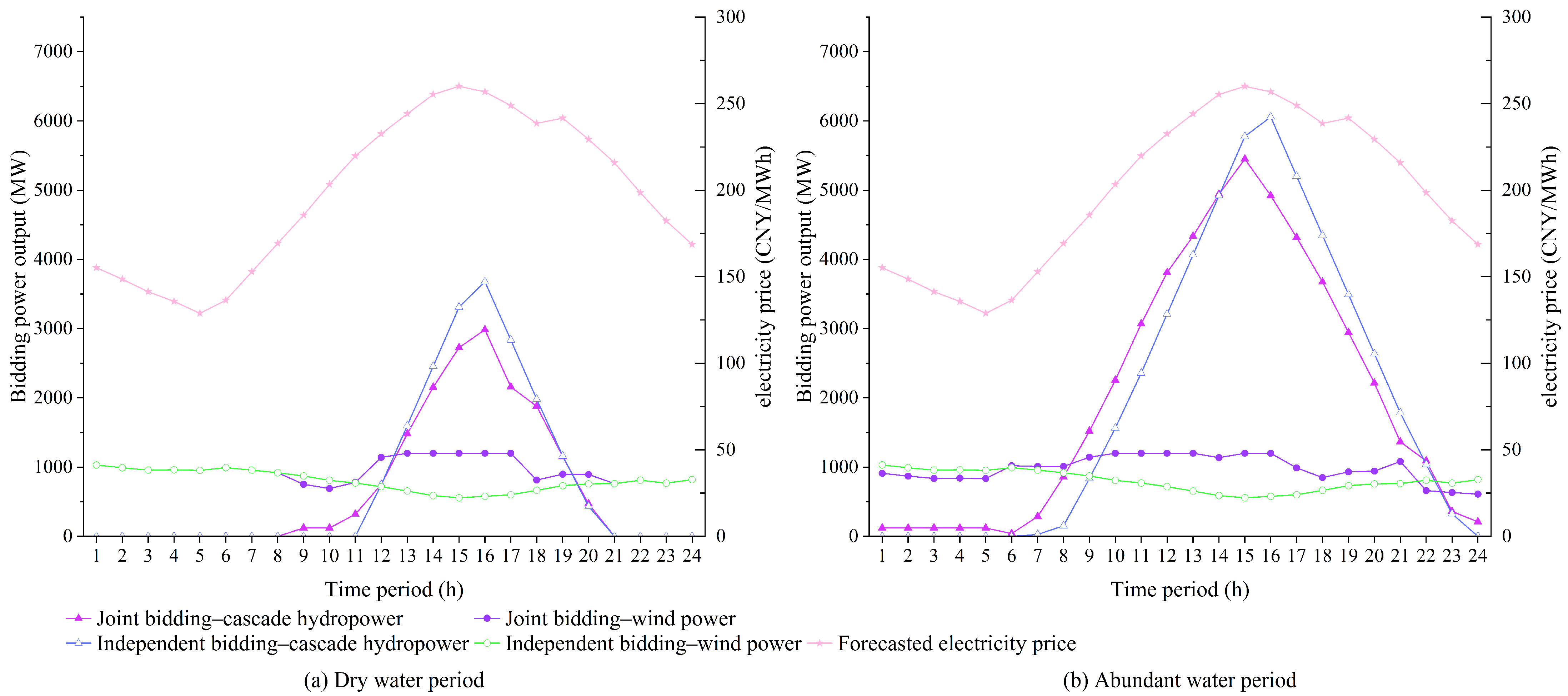
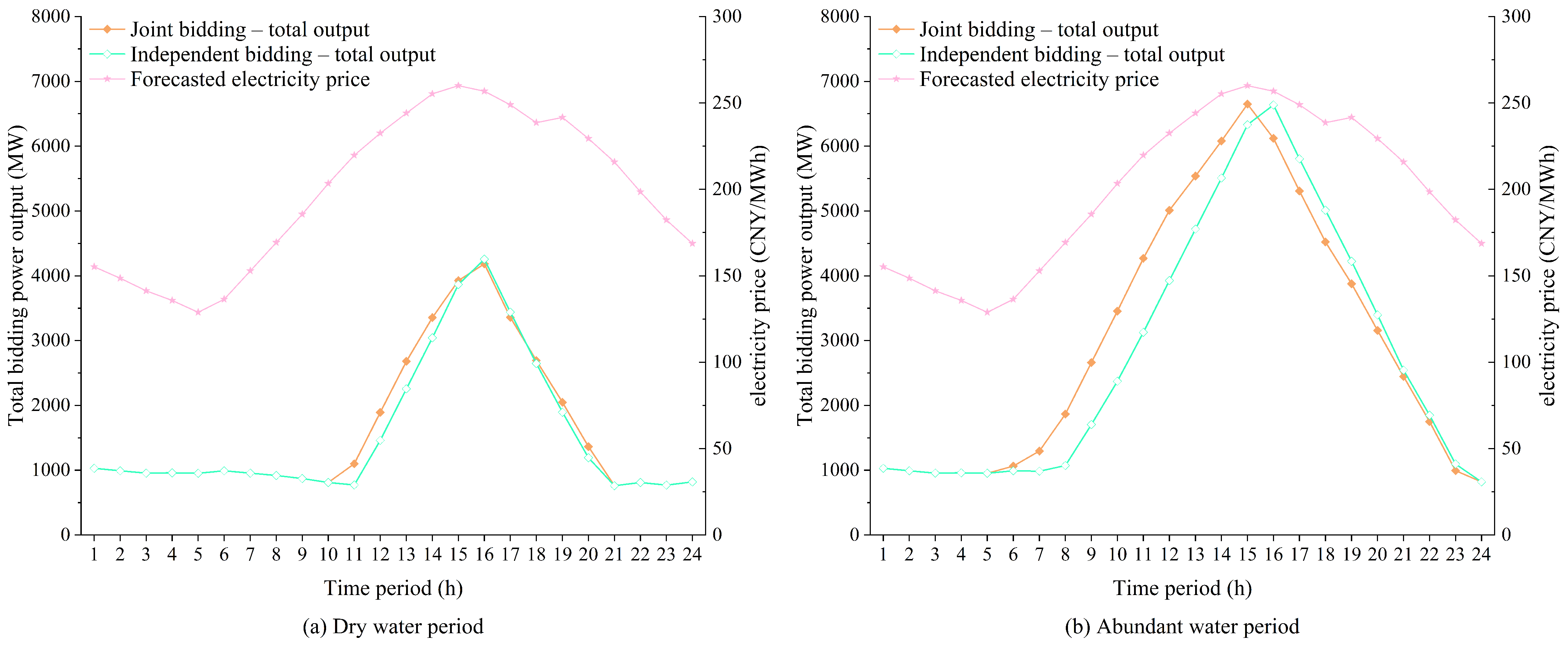
Under dry water period conditions, as shown in Figure 5a, the overall regulation capability of the cascade hydropower system is relatively limited due to constrained inflows, and its bidding output is mainly concentrated in periods with relatively high electricity prices (t = 12–20). During low-price periods (t = 1–8), cascade hydropower does not submit bids under either joint bidding or non-joint bidding schemes, as insufficient effective water resources are available for real-time market regulation at this stage; accordingly, wind power bidding outputs under joint and non-joint bidding are almost identical in this interval. In the high-price period (t = 12–20), wind power bidding output under joint bidding is significantly higher than that under non-joint bidding, whereas the bidding output of cascade hydropower is relatively reduced and exhibits a smoother trajectory. In contrast, under non-joint bidding, cascade hydropower shows pronounced and concentrated peak bidding behavior during t = 13–17. Combined with the total bidding output results in Figure 6a, it can be observed that under dry water period conditions, joint bidding yields a slightly higher total output during the price ramp-up phase. Overall, when the regulation capability of cascade hydropower is limited, joint bidding effectively reallocates the temporal structure of hydropower and wind power bidding outputs, enabling limited bidding volumes to be more efficiently allocated to high-price periods, thereby avoiding excessive concentration of bidding volumes solely relying on cascade hydropower during peak hours and ultimately enhancing overall revenue performance.

Under abundant water period conditions, as shown in Figure 5b, cascade hydropower benefits from abundant inflows and a markedly enhanced regulation capability, making the structural advantages of hydro–wind joint bidding more evident. During low-price periods (t = 1–5 and t = 22–24), wind power bidding output under joint bidding is overall slightly lower than that under non-joint bidding, while cascade hydropower output remains at a relatively low level. In high-price periods (t = 9–21), wind power bidding output under joint bidding is significantly higher than that under non-joint bidding, and meanwhile, the bidding output of cascade hydropower exhibits a smoother ramping pattern following price variations. Under abundant water period conditions, joint bidding increases wind power bidding output during high-price intervals; moreover, as indicated by the total bidding output in Figure 6b, joint bidding enables a faster formation of larger bidding volumes during the price uptrend, allowing the overall output trajectory to align more closely with the electricity price dynamics.

By jointly considering the results under dry water period and abundant water period conditions, it can be observed that wind power output exhibits a certain anti-peak characteristic in some periods, where high output intervals are often misaligned with electricity price peak periods. The introduction of cascade hydropower effectively alleviates this structural mismatch, enabling the hydro–wind alliance to maintain relatively high bidding output during electricity price peak periods, thereby enhancing the overall responsiveness of the joint bidding strategy to market price signals.

4.1.2. Expected Revenue, CVaR, and Revenue Distribution Characteristics Analysis

Table 4. Bidding revenue and CVaR under the risk-neutral condition (β = 0).

Bidding Strategy	Risk-Neutral (β = 0)
	Expected Bidding Revenue (Thousand CNY)		CvaR (Thousand CNY)
	Dry Water Period	Abundant Water Period	Dry Water Period	Abundant Water Period
Joint bidding	8568.78	16,059.68	8111.16	15,336.55
Hydropower independent bidding	4557.24	11,507.80	4302.69	10,961.98
Wind power independent bidding	3582.86	3582.86	3377.38	3377.38
Sum of separate bidding	8140.10	15,090.66	7680.07	14,339.36
Incremental benefit	428.68	969.02	431.09	997.19
Allocated revenue of hydropower	4771.58	11,992.31
Allocated revenue of wind power	3797.20	4067.37

presents the bidding revenue results under the risk-neutral condition. Under dry water period conditions, the expected revenue of joint bidding reaches 8568.78 thousand CNY, which is higher than the sum of revenues obtained from separate bidding, i.e., 8140.10 thousand CNY, resulting in an increase of 428.68 thousand CNY; correspondingly, the CVaR increases from 7680.07 thousand CNY to 8111.16 thousand CNY, with an improvement of 431.09 thousand CNY. Under abundant water period conditions, the joint bidding revenue reaches 16,059.68 thousand CNY, representing an increase of 969.02 thousand CNY compared with the sum of separate bidding revenues, while the CVaR is improved by 997.19 thousand CNY. These results indicate that hydro–wind joint bidding can not only enhance the expected revenue level but also effectively improve the risk–return performance.

The revenue allocation results based on the Shapley value method show that the incremental revenue brought by joint bidding is distributed fairly and reasonably between hydropower and wind power. Under both dry water and abundant water period conditions, the allocated revenues of hydropower and wind power under joint bidding are higher than their respective revenues obtained from separate bidding. This indicates that although hydropower needs to undertake certain regulation responsibilities in the joint bidding process and may give up part of its standalone revenue potential, the Shapley value-based allocation mechanism can effectively compensate for the regulation cost of hydropower while enhancing the participation incentives of wind power in bidding.

To further illustrate the distributional characteristics of bidding revenue,

Table 5. Scenario-based statistics of bidding revenue under the risk-neutral condition.

Bidding Strategy	Bidding Revenue Distribution (Thousand CNY) Risk-Neutral (β = 0)
	Standard Deviation		Maximum Revenue		Minimum Revenue
	Dry	Abundant	Dry	Abundant	Dry	Abundant
Joint bidding	318.92	555.08	9036.18	16,802.94	8111.16	15,337.34
Hydropower independent bidding	216.58	455.57	4852.49	12,091.45	4302.69	10,961.98
Wind power independent bidding	136.62	136.62	3844.11	3844.11	3377.38	3377.38
Sum of separate bidding			8696.60	15,935.56	7680.07	14,339.36

presents the scenario-based standard deviation together with the maximum and minimum revenues under the representative scenarios. It can be observed that, under both hydrological conditions, the complementary regulation between cascade hydropower and wind power enables joint bidding to maintain a revenue level higher than the sum of separate bidding revenues in both favorable and unfavorable scenarios.

4.1.3. Supplementary Analysis with Additional Extreme Scenarios

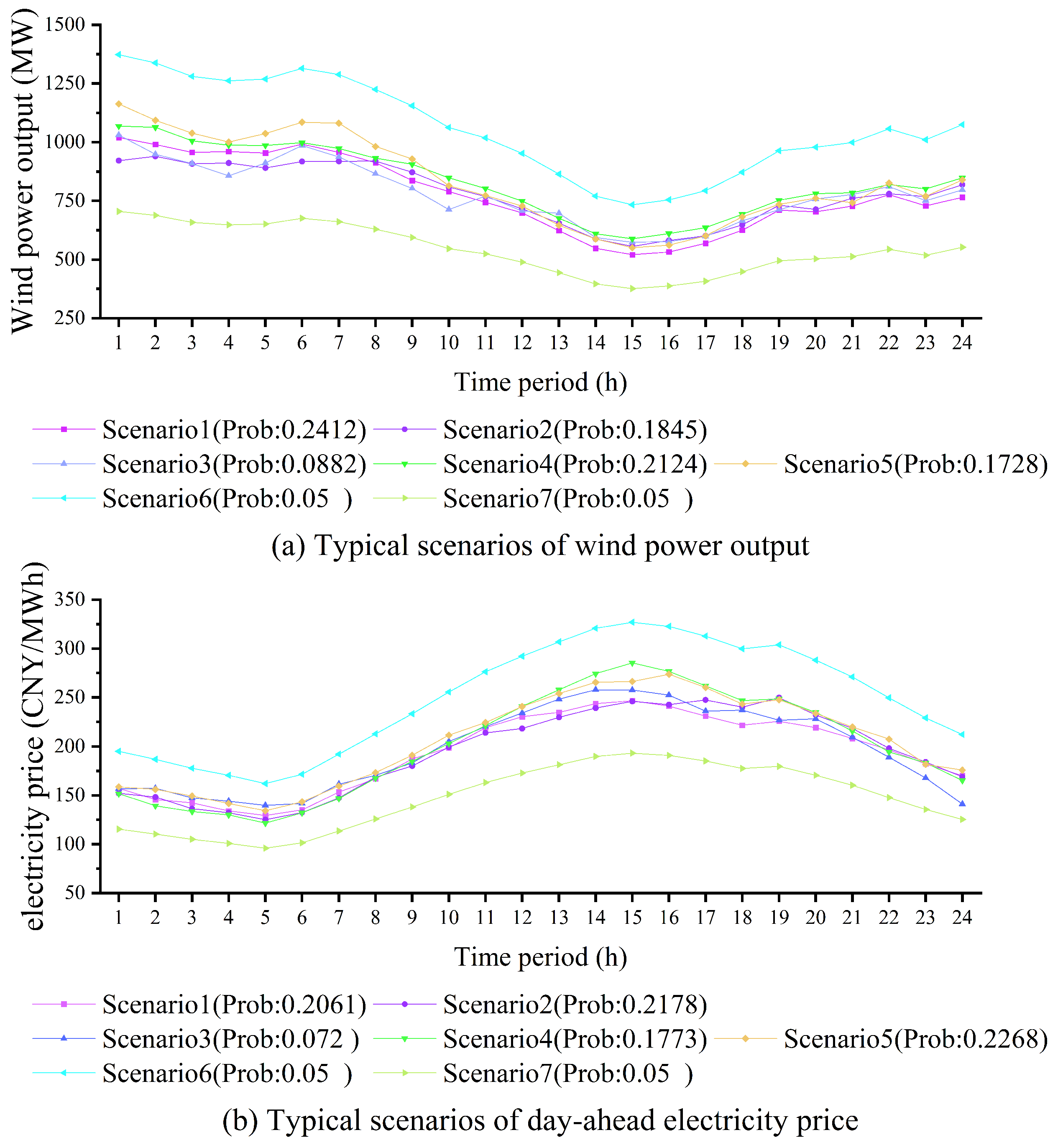
To examine the impact of additional extreme scenarios on bidding results, this subsection supplements the representative scenario set with lower-tail and upper-tail scenarios, as shown in Figure 7. Specifically, for each uncertain variable, i.e., wind power output and day-ahead electricity price, one lower-tail scenario and one upper-tail scenario are constructed from the samples located in the lower- and upper-quantile regions, respectively, based on a large number of original scenarios generated by Latin hypercube sampling (LHS). As a result, the number of representative scenarios for each variable increases from 5 to 7, and the number of joint scenarios increases from 25 to 49 after the Cartesian product combination. The added extreme scenarios are assigned small probabilities, while the probabilities of the original representative scenarios are proportionally adjusted to maintain normalization. In this way, the revenue and CVaR results can be further examined with a more explicit representation of tail events.

The corresponding results are summarized in

Table 6. Bidding revenue and CVaR under the risk-neutral condition with additional extreme scenarios.

Bidding Strategy	Risk-Neutral (β = 0)
	Expected Bidding Revenue (Thousand CNY)		CVaR (Thousand CNY)
	Dry Water Period	Abundant Water Period	Dry Water Period	Abundant Water Period
Joint bidding	8505.56	15,996.17	6335.54	13,079.95
Hydropower independent bidding	4557.05	11,507.61	4123.54	10,491.08
Wind power independent bidding	3519.94	3519.94	1930.76	1930.76
Sum of separate bidding	8076.99	15,027.55	6054.30	12,421.84
Incremental benefit	428.57	968.62	281.24	658.11
Allocated revenue of hydropower	4771.34	11,991.92
Allocated revenue of wind power	3734.22	4004.25

. After the additional lower- and upper-extreme scenarios are introduced, the expected revenues of all bidding strategies decrease slightly under both hydrological conditions, whereas the CVaR values decrease more markedly. For joint bidding, the expected revenue decreases from 8568.78 to 8505.56 thousand CNY in the dry water period and from 16,059.68 to 15,996.17 thousand CNY in the abundant water period. Meanwhile, the corresponding CVaR decreases from 8111.16 to 6335.54 thousand CNY and from 15,336.55 to 13,079.95 thousand CNY, respectively. This suggests that, after the additional extreme scenarios are incorporated, the lower-tail outcomes of bidding revenue are more fully captured in the evaluation. Although upper-extreme scenarios are also included, the adverse impact of the additional lower-tail scenarios on revenue is stronger than the positive offset brought by the upper-tail scenarios, leading to a slight decline in expected revenue and a more pronounced decline in CVaR.

Table 7. Scenario-based statistics of bidding revenue under the risk-neutral condition with additional extreme scenarios.

Bidding Strategy	Bidding Revenue Distribution (Thousand CNY) Risk-Neutral (β = 0)
	Standard Deviation		Maximum Revenue		Minimum Revenue
	Dry	Abundant	Dry	Abundant	Dry	Abundant
Joint bidding	861.20	1462.39	11,450.69	20,857.11	5035.47	10,607.48
Hydropower independent bidding	423.28	1029.80	5725.64	14,461.72	3385.09	8550.01
Wind power independent bidding	523.21	523.21	5190.38	5190.38	1320.68	1320.68
Sum of separate bidding			10,916.02	19,652.10	4705.77	9870.69

further reports the scenario-based revenue statistics when extreme scenarios are considered. Compared with the baseline 25-scenario case, the dispersion of bidding revenue increases significantly after the additional extreme scenarios are introduced. For example, under joint bidding, the standard deviation increases from 318.92 to 861.20 thousand CNY in the dry water period and from 555.08 to 1462.39 thousand CNY in the abundant water period, while the revenue range between the maximum and minimum values also widens substantially. This indicates that considering additional extreme scenarios can reveal a wider range of revenue fluctuations and tail outcomes. Overall, after the additional extreme scenarios are incorporated, the revenue levels and downside-risk indicators change noticeably, while the main comparative finding of the case study remains the same: joint bidding still shows a clear economic advantage over the separate-bidding benchmark under both hydrological conditions.

4.2. Comparative Analysis of Different Cases

This section compares different configuration schemes of joint bidding under the risk-neutral condition (β = 0). Three case scenarios are considered: Case A considers vibration zone avoidance and introduces penalties for vibration zone crossing; Case B considers only vibration zone avoidance; and Case C does not consider vibration zones. Under the risk-neutral condition (β = 0), the joint bidding results of the three cases are analyzed, as summarized in

Table 8. Comparative results of different cases.

Case	Expected Bidding Revenue (Thousand CNY)		Number of Vibration Zone Crossings in the Day-Ahead Stage		Number of Vibration Zone Crossings Caused by Real-Time Deviation Adjustment
	Dry Water Period	Abundant Water Period	Dry Water Period	Abundant Water Period	Dry Water Period	Abundant Water Period
Case A	8568.78	16,059.68	10	9	0	25
Case B	8578.90	16,069.76	10	12	220	275
Case C	8580.70	16,073.40	—	—	—	—

. From the perspective of economic performance, Case C achieves the highest expected bidding revenue in both the dry water period and the abundant water period, reaching 8580.70 thousand CNY and 16,073.40 thousand CNY, respectively; Case B ranks second, while Case A yields slightly lower revenues. Specifically, compared with Case C, the expected revenue of Case A decreases by 11.92 thousand CNY in the dry water period (approximately 0.14%) and by 13.72 thousand CNY in the abundant water period (approximately 0.09%); compared with Case B, the expected revenue of Case A decreases by 10.12 thousand CNY in the dry water period (approximately 0.12%) and by 10.08 thousand CNY in the abundant water period (approximately 0.06%). These results indicate that incorporating vibration zone avoidance and introducing penalties for vibration zone crossing has a relatively small impact on joint bidding revenue, and the overall economic performance remains stable.

However, from the perspective of operational safety, clear differences can be observed among the three cases. Although Case B yields slightly higher revenue than Case A, it does not consider vibration zone crossing. In the day-ahead stage, during the dry water period, the number of vibration zone crossings of hydropower bidding output is both 10 for Case B and Case A; during the abundant water period, the corresponding numbers are 12 for Case B and 9 for Case A. In the real-time deviation adjustment process, the number of vibration zone crossings under Case B is 220 in the dry water period and 275 in the abundant water period. In contrast, under Case A, the corresponding numbers are 0 in the dry water period and 25 in the abundant water period, which are 220 and more than 250 fewer, respectively, than those under Case B. Case C does not consider hydropower vibration zones, and the corresponding numbers are not reported; however, its potential operational risk is difficult to evaluate and it does not meet the basic safety requirements of practical operation.

By jointly considering economic performance and hydropower operational safety, Case A effectively suppresses the frequency of vibration zone crossings of hydropower units in both the day-ahead bidding and real-time adjustment processes at the cost of less than 0.2% loss in expected revenue, thereby achieving an effective balance between economic benefits and operational safety. In comparison, although Case B exhibits a slight revenue advantage, its substantially higher frequency of vibration zone crossings is unfavorable for the healthy operation of hydropower units. Case C, despite yielding the highest theoretical revenue, neglects vibration zone–related factors and thus faces greater operational risks in practical applications. Therefore, when both bidding revenue and hydropower operational safety are taken into account, Case A demonstrates superior overall performance.

4.3. Risk Preference Analysis

To examine how decision-makers’ risk preferences affect joint bidding outcomes, β is treated as an exogenous preference parameter and varied from 0.1 to 1.0 with a step size of 0.1. The bidding revenue and CVaR of joint bidding under dry water period conditions are analyzed accordingly.

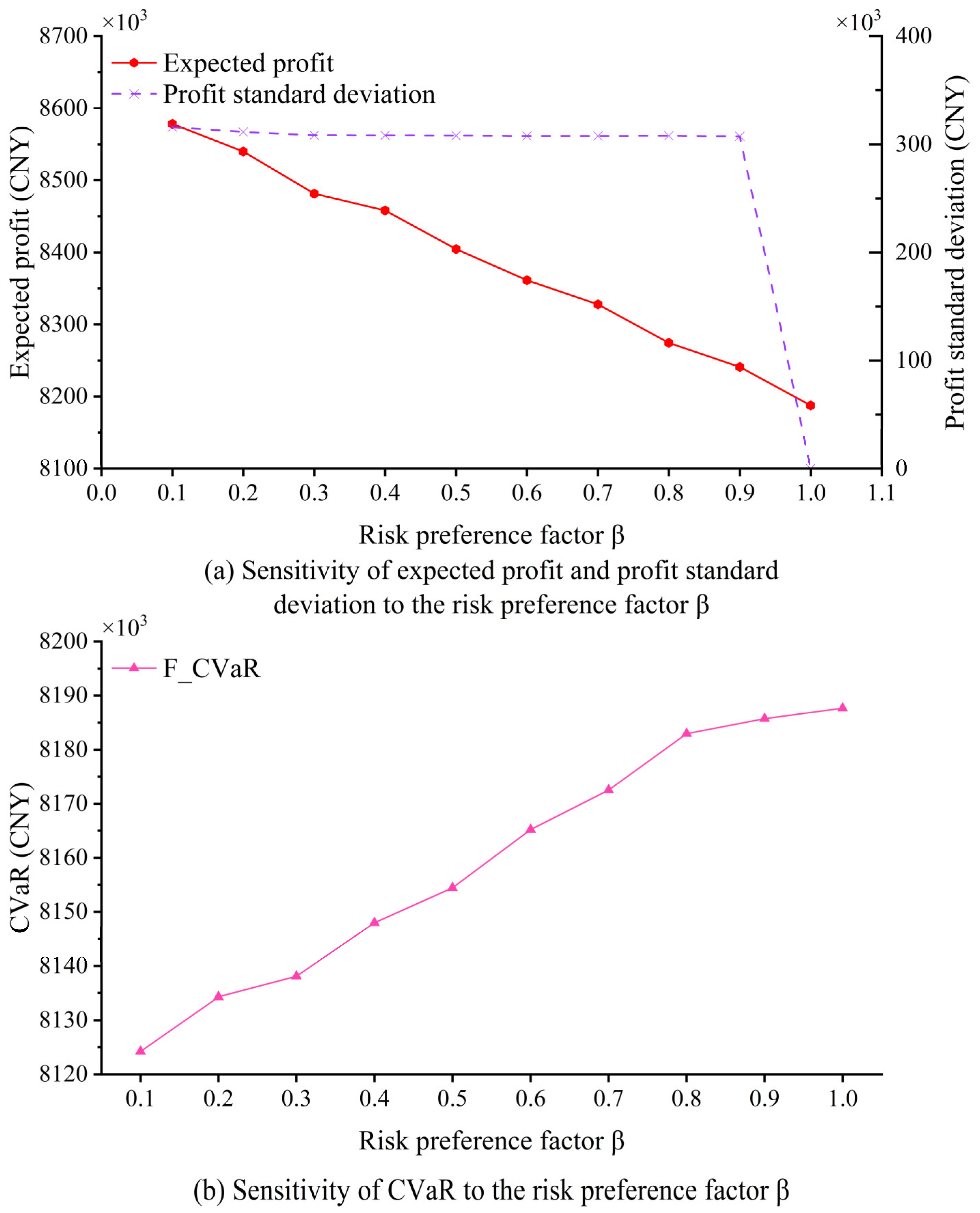
Figure 8a,b compares the variations in expected revenue, revenue standard deviation, and CVaR of the alliance under different values of the risk factor β. As shown in Figure 8a, the expected bidding revenue exhibits an overall monotonic decreasing trend as β increases; when β increases from 0.1 to 0.9, the expected revenue decreases from approximately 8578.26 thousand CNY to approximately 8187.67 thousand CNY, indicating that greater risk aversion leads to more conservative bidding strategies and a lower revenue level. Over the same range, however, the revenue standard deviation remains nearly unchanged. This is mainly because, under moderate risk-aversion levels, the natural complementarity between cascade hydropower regulation and wind power effectively absorbs a large part of the revenue fluctuations caused by wind power uncertainty. At the same time, physical constraints such as water availability and ramping limits continue to restrict further adjustment of the bidding strategy, leaving limited room for β to further reduce overall revenue volatility. When β reaches 1.0, the model places substantially greater emphasis on downside-risk control, and the resulting bidding strategy becomes noticeably more conservative. Consequently, the revenue standard deviation decreases more visibly.

Figure 8b illustrates the variation in CVaR with respect to the risk factor β. As β increases, CVaR exhibits a monotonic increasing trend, rising from approximately 8124.25 thousand CNY to approximately 8187.67 thousand CNY, indicating that the model places progressively greater emphasis on unfavorable tail scenarios and improves revenue performance in the worst 5% of cases. Meanwhile, when β takes relatively large values (e.g., β ≥ 0.8), the increase in CVaR becomes less pronounced, mainly because the potential for further improvement in tail revenue is constrained by physical limits such as water availability and ramping constraints.

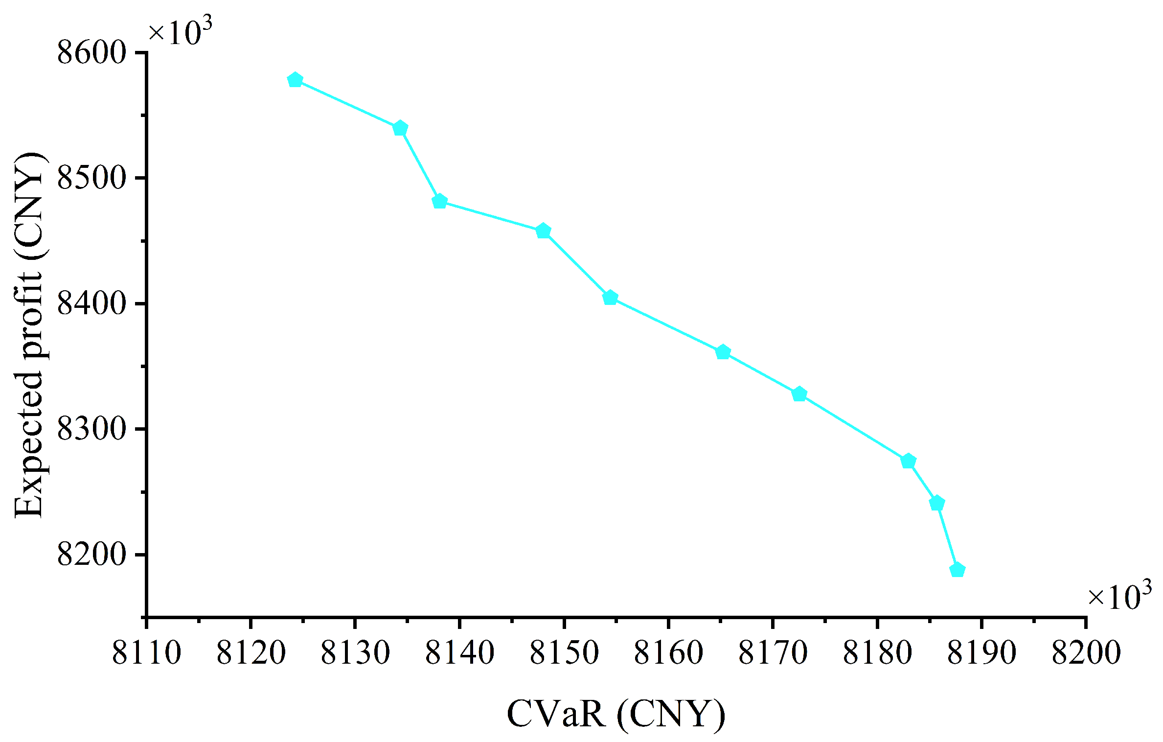
Figure 9 presents the efficient frontier formed by the expected revenue and CVaR of the joint bidding strategy as the risk factor β varies over the range from 0.1 to 1.0. Each square marker in the figure corresponds to the expected revenue and risk level under a specific value of β, reflecting the trade-off relationship between joint bidding revenue and tail risk.

Based on the above analysis, it can be concluded that the risk factor β plays a significant trade-off role between expected revenue and risk control. As β increases, the alliance reduces revenue volatility and improves tail revenue levels at the cost of sacrificing part of the expected revenue, thereby enhancing the robustness of the bidding strategy under uncertainty. These results demonstrate that introducing a CVaR-based risk measurement mechanism can guide the hydro–wind alliance to form bidding decisions that better align with risk preferences, providing a flexible and adjustable decision-making tool for market participants with different risk tolerance levels. To further illustrate how different risk preferences are reflected in actual bidding decisions, Section 4.4 presents a comparative analysis of the total bidding output and deviation output under different risk preference settings.

4.4. Impact of Decision-Maker Risk Preference on Bidding Strategy

This section takes the abundant water period as a case study to compare hydro–wind joint bidding strategies under different risk preferences. The risk factor is set to β = 0 (risk-neutral) and β = 0.5 (risk-averse), respectively, to investigate the impact of different risk preferences on joint bidding decision outcomes.

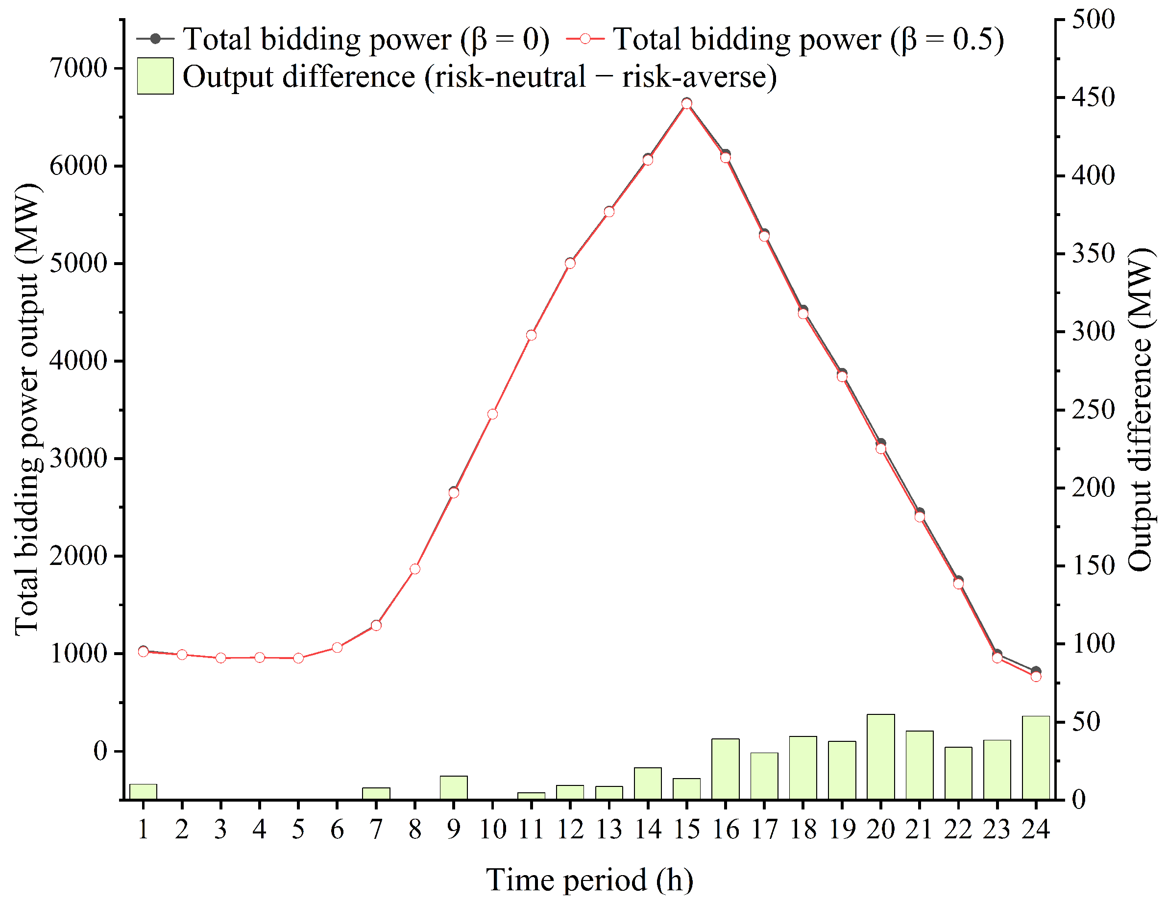
By comparing the day-ahead total bidding output under the risk-neutral case (β = 0, black) and the risk-averse case (β = 0.5, red) in Figure 10, it can be observed that during some price valley periods (t = 1, 7, 9) and most peak periods (t = 14–24), the total bidding output under the risk-averse condition is generally slightly lower than that under the risk-neutral condition. The bar differences shown in the figure (“risk-neutral − risk-averse”) are mostly positive, indicating that the bidding strategy under risk aversion adopts a more conservative submission approach in most time periods.

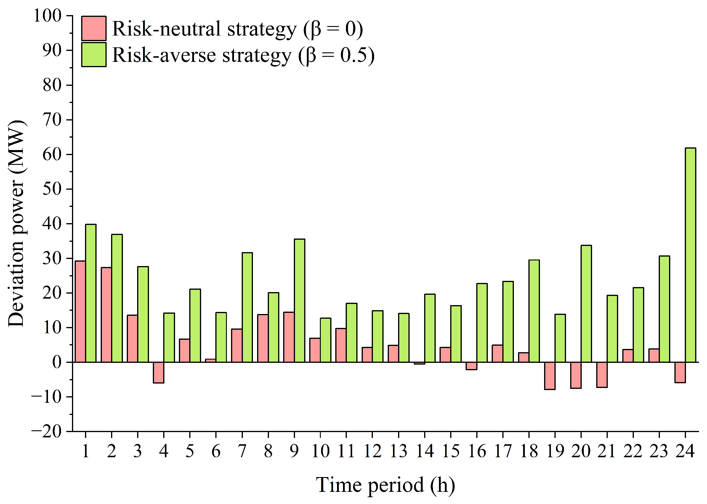
Figure 11 presents a comparison of the deviation outputs of joint bidding at each time period under the risk-neutral (β = 0) and risk-averse (β = 0.5) conditions. As shown in the figure, under the risk-neutral strategy, the deviation output is mainly positive, with negative deviations occurring only in a few time periods; under the risk-averse strategy, the deviations at all time periods are positive, and the magnitudes of positive deviations in most periods are higher than those under the risk-neutral case. Considering the deviation settlement mechanism, positive deviation energy is settled at a positive deviation price lower than the day-ahead electricity price, resulting in a relatively limited impact on revenue, whereas negative deviation energy is settled at a negative deviation price higher than the day-ahead electricity price, which significantly reduces joint bidding revenue and amplifies tail risk. Therefore, under the risk-averse strategy, the alliance tends to reduce the submitted quantity in the day-ahead stage and increase the fulfillment margin, making real-time output more likely to be close to or higher than the day-ahead submission, thereby avoiding penalties caused by insufficient energy when real-time output falls below the day-ahead bid.

As shown in

Table 9. Comparison of bidding revenue and CVaR under different risk preferences.

Case	Abundant Water Period
	Expected Revenue (Thousand CNY)	CVaR (Thousand CNY)
Risk-neutral (β = 0)	16,059.68	15,336.55
Risk-Averse (β = 0.5)	15,726.32	15,394.82
Difference	−333.36	58.27

, in the abundant water period case study, the risk factor β has a significant impact on the revenue structure of joint bidding. When β = 0 (risk-neutral), the expected revenue is 16,059.68 thousand CNY and the CVaR is 15,336.55 thousand CNY. When β increases to 0.5 (risk-averse), the expected revenue decreases to 15,726.32 thousand CNY, with a reduction of 333.36 thousand CNY, while the CVaR increases to 15,394.82 thousand CNY, with an increase of 58.27 thousand CNY. Overall, although the risk-neutral bidding strategy yields higher bidding revenue, it is accompanied by higher tail risk, whereas the risk-averse strategy results in lower bidding revenue while exhibiting lower uncertainty-related risk.

5. Conclusions

This paper develops a two-stage joint bidding model for cascade hydropower and wind power that incorporates the decision-maker’s risk preference. By leveraging the flexible regulation capability of cascade hydropower, the proposed model offsets the uncertainty of wind power output, thereby improving joint bidding revenue and bid fulfillment performance. The model introduces Conditional Value-at-Risk (CVaR) and a risk factor to coordinate the trade-off between revenue and risk. Meanwhile, the operational characteristics of cascade hydropower are fully considered by dividing the output range into safe operating zones to achieve vibration zone avoidance, introducing penalty terms in the objective function to suppress vibration zone crossing behavior, and employing piecewise linearization to handle dynamic water flow delay constraints. Based on an empirical study of a cascade hydropower system and a wind farm in southwestern China, the following conclusions are obtained:

(1)

The proposed CVaR-based risk-aware bidding framework can effectively characterize the trade-off between expected revenue and downside risk. As the risk factor increases, the alliance adopts more conservative bidding strategies, which reduces expected revenue while improving CVaR performance. This provides flexible decision-making support for market participants with different risk tolerance levels.

(2)

Joint bidding outperforms non-joint bidding in both revenue level and tail risk performance. In both the dry water period and abundant water period case studies, the regulation capability of cascade hydropower mitigates wind power deviations, reducing imbalance energy and the associated penalty costs, thereby increasing overall joint bidding revenue and improving CVaR performance.

(3)

Incorporating vibration zone factors as operational constraints and penalty terms can suppress crossing behavior with limited revenue impact. Vibration zone avoidance constraints ensure that hydropower output remains within safe operating zones, while vibration zone crossing penalties in the objective function further reduce the frequency of vibration zone crossings, thereby lowering potential operational risks and making the joint bidding scheme more consistent with unit safety requirements.

This study is developed within a price-taker framework and focuses on quantity-based bidding decisions under exogenous electricity price scenarios, which helps highlight the effects of hydro–wind complementarity, risk preference, and hydropower operational constraints on joint bidding outcomes. More strategic market settings may be further investigated in future work. In particular, for market environments in which the alliance may exert non-negligible market influence, the model can be extended to a price-maker framework to explicitly capture the interaction between bidding decisions and market-clearing results. In addition, stepwise bidding structures may be incorporated to represent more flexible price–quantity offering behaviors. Furthermore, although the present scalarized formulation is computationally convenient for the proposed two-stage stochastic MILP and allows intuitive sensitivity analysis of risk preference, alternative multi-objective methods, such as reference-point-based or ε-constraint formulations, may provide a more systematic exploration of non-dominated bidding solutions. These extensions, together with multi-stage and multi-market decision frameworks involving medium- and long-term contracts, ancillary services, and additional uncertainties such as inflow, load, and electricity prices, will be considered in future research.

References

1. Li, X. Nine Departments Including the National Development and Reform Commission Issue the “14th Five-Year Plan for Renewable Energy Development”. China Equip. Eng. 2022, 13, 1. [Google Scholar]
2. State Council Information Office of the People’s Republic of China. Carbon Peaking and Carbon Neutrality: China’s Actions. Available online: http://english.www.gov.cn/archive/whitepaper/202511/08/content_WS690ee812c6d00ca5f9a076cd.html (accessed on 16 January 2026).
3. Xie, K.; Liu, D.; Li, Z.; Sun, T.; Pang, B.; Liu, S.; Zhang, X. Multi-Dimensional Collaborative Electricity Market System for New Power System. Autom. Electr. Power Syst. 2024, 48, 2–12. [Google Scholar]
4. Xiao, Y.; Zou, C.; Dong, M.; Chi, H.; Yan, Y.; Jiang, S. Feasibility Study: Economic and Technical Analysis of Optimal Configuration and Operation of a Hybrid CSP/PV/Wind Power Cogeneration System with Energy Storage. Renew. Energy 2024, 225, 120273. [Google Scholar] [CrossRef] [Scilit]
5. Wu, Z.; Zhou, M.; Li, G.; Zhao, T.; Zhang, Y.; Liu, X. Interaction between Balancing Market Design and Market Behaviour of Wind Power Producers in China. Renew. Sustain. Energy Rev. 2020, 132, 110060. [Google Scholar] [CrossRef] [Scilit]
6. Ahmed, S.D.; Al-Ismail, F.S.M.; Shafiullah, M.; Al-Sulaiman, F.A.; El-Amin, I.M. Grid Integration Challenges of Wind Energy: A Review. IEEE Access 2020, 8, 10857–10878. [Google Scholar] [CrossRef] [Scilit]
7. Wang, H.; Sun, W.; Sang, B. Spot Market Bidding Strategy for a “Renewable Energy + Energy Storage” Power Station Considering Conditional Value at Risk. Power Syst. Technol. 2023, 47, 3620–3628. [Google Scholar]
8. Khaloie, H.; Abdollahi, A.; Shafie-Khah, M.; Anvari-Moghaddam, A.; Nojavan, S.; Siano, P.; Catalão, J.P.S. Coordinated Wind–Thermal–Energy Storage Offering Strategy in Energy and Spinning Reserve Markets Using a Multi-Stage Model. Appl. Energy 2020, 259, 114168. [Google Scholar] [CrossRef] [Scilit]
9. Khaloie, H.; Abdollahi, A.; Shafie-Khah, M.; Siano, P.; Nojavan, S.; Anvari-Moghaddam, A.; Catalão, J.P.S. Co-Optimized Bidding Strategy of an Integrated Wind–Thermal–Photovoltaic System in Deregulated Electricity Market under Uncertainties. J. Clean. Prod. 2020, 242, 118434. [Google Scholar] [CrossRef] [Scilit]
10. Jin, X.; Liu, B.; Liao, S.; Cheng, C.; Jurasz, J.; Zhang, Y.; Lu, J. Exploring the Transition Role of Cascade Hydropower in 100% Decarbonized Energy Systems. Energy 2023, 279, 128086. [Google Scholar] [CrossRef] [Scilit]
11. Li, X.; Yang, W.; Liao, Y.; Zhang, S.; Zheng, Y.; Zhao, Z.; Tang, M.; Cheng, Y.; Liu, P. Short-Term Risk-Management for Hydro–Wind–Solar Hybrid Energy System Considering Hydropower Part-Load Operating Characteristics. Appl. Energy 2024, 360, 122818. [Google Scholar] [CrossRef] [Scilit]
12. Liu, B.; Liu, T.; Liao, S.; Lu, J.; Cheng, C. Short-Term Coordinated Hybrid Hydro–Wind–Solar Optimal Scheduling Model Considering Multistage Section Restrictions. Renew. Energy 2023, 217, 119160. [Google Scholar] [CrossRef] [Scilit]
13. Li, H.; Li, X.; Zhang, Y.; Zhao, Y.; Pan, J.; Zhao, H. Declaration Strategy of Wind Power and Pumped Storage Participating in the Power Market Considering Multiple Uncertainties. Energy 2024, 293, 130624. [Google Scholar] [CrossRef] [Scilit]
14. Tan, Q.; Wen, X.; Sun, Y.; Lei, X.; Wang, Z.; Qin, G. Evaluation of the Risk and Benefit of the Complementary Operation of the Large Wind–Photovoltaic–Hydropower System Considering Forecast Uncertainty. Appl. Energy 2021, 285, 116442. [Google Scholar] [CrossRef] [Scilit]
15. Xu, Y.; Jiang, Z.; Peng, W.; Lu, P.; Wang, J.; Xu, Y.; Lu, J. Multi-Objective Optimization and Mechanism Analysis of Integrated Hydro–Wind–Solar–Storage System: Based on Medium-Long-Term Complementary Dispatching Model Coupled with Short-Term Power Balance. Energy 2025, 332, 137246. [Google Scholar] [CrossRef] [Scilit]
16. Zhao, H.; Liao, S.; Ma, X.; Fang, Z.; Cheng, C.; Zhang, Z. Short-Term Peak-Shaving Scheduling of a Hydropower-Dominated Hydro–Wind–Solar Photovoltaic Hybrid System Considering a Shared Multienergy Coupling Transmission Channel. Appl. Energy 2024, 372, 123786. [Google Scholar] [CrossRef] [Scilit]
17. Wang, Y.; Zhao, M.; Chang, J.; Wang, X.; Tian, Y. Study on the Combined Operation of a Hydro–Thermal–Wind Hybrid Power System Based on Hydro–Wind Power Compensating Principles. Energy Convers. Manag. 2019, 194, 94–111. [Google Scholar] [CrossRef] [Scilit]
18. Cerejo, A.; Mariano, S.J.P.S.; Carvalho, P.M.S.; Calado, M.R.A. Hydro–Wind Optimal Operation for Joint Bidding in Day-Ahead Market: Storage Efficiency and Impact of Wind Forecasting Uncertainty. J. Mod. Power Syst. Clean Energy 2020, 8, 142–149. [Google Scholar] [CrossRef] [Scilit]
19. Xiao, Y.; Li, C.; Li, S.; Zhu, Q.; Chang, P.; Wu, T. Bidding–Clearing–Scheduling Coordinated Optimization for Cascade Hydro–Wind–Photovoltaic Alliances in Electricity Spot Markets: A Multi-Stage Framework. Energy 2025, 335, 138185. [Google Scholar] [CrossRef] [Scilit]
20. Li, Y.; Fang, N.; He, S.; Wu, F.; Li, O.; Shi, L.; Ding, R. Two-Stage Stochastic Scheduling of Cascaded Hydropower–Wind–Photovoltaic Hybrid Systems Considering Contract Decomposition and Spot Market. Sustainability 2024, 16, 1093. [Google Scholar] [CrossRef] [Scilit]
21. Li, X.; Liu, P.; Cheng, L.; Cheng, Q.; Zhang, W.; Xu, S.; Zheng, Y. Strategic Bidding for a Hydro–Wind–Photovoltaic Hybrid System Considering the Profit beyond Forecast Time. Renew. Energy 2023, 204, 277–289. [Google Scholar] [CrossRef] [Scilit]
22. Bai, Q.; Zhao, Z.; Jin, X.; Cheng, C.; Deng, Z.; Jia, Z. Hydro–Wind Power Joint Bidding Strategies for Electricity Spot Market Considering Uncertainties of Wind Power Output and Electricity Price. Autom. Electr. Power Syst. 2024, 48, 122–133. [Google Scholar]
23. Aydoğdu, A.; Tör, O.B.; Güven, A.N. CVaR-based stochastic wind-thermal generation coordination for Turkish electricity market. J. Mod. Power Syst. Clean Energy 2019, 7, 1307–1318. [Google Scholar] [CrossRef] [Scilit]
24. Wang, Y.; Wang, J.; Sun, W.; Zhao, M. Optimal day-ahead bidding strategy for electricity retailer with inner-outer 2-layer model system based on stochastic mixed-integer optimization. Math. Probl. Eng. 2019, 2019, 4185952. [Google Scholar] [CrossRef] [Scilit]
25. Zoltowska, I. Risk Preferences of EV Fleet Aggregators in Day-Ahead Market Bidding: Mean-CVaR Linear Programming Model. Energies 2025, 18, 93. [Google Scholar] [CrossRef] [Scilit]
26. He, M.; Han, S.; Chen, D.; Zhao, Z.; Jurasz, J.; Mahmud, A.; Liu, P.; Deng, M. Optimizing Cascade Hydropower–VRE Hybrid Systems: A Novel Approach Addressing Whole-Process Vibration to Enhance Operational Safety. Energy 2024, 304, 131965. [Google Scholar] [CrossRef] [Scilit]
27. Wang, X.; Gao, C. Two-Stage Decision-Making Model of Power Generation and Coal Purchase Arrangement for Power Generation Companies in Medium- and Long-Term Market. Power Syst. Technol. 2021, 45, 3992–3999. [Google Scholar]
28. Su, C.; Wang, P.; Wu, X. A Compact MILP Model for Short-Term Peak Shaving of Cascaded Hydropower Plants Considering Unit Commitment. Power Syst. Technol. 2018, 42, 1883–1891. [Google Scholar]
29. Yu, S.; Fang, F.; Liu, Y.; Liu, J. Uncertainties of Virtual Power Plant: Problems and Countermeasures. Appl. Energy 2019, 239, 454–470. [Google Scholar] [CrossRef] [Scilit]
Figure 1. Decision-making framework.
Energies 19 01545 g001
Figure 2. Flowchart of the K-Means clustering process. Arrows indicate the workflow sequence and iterative loop, and the superscript “*” denotes the final converged results.
Energies 19 01545 g002
Figure 3. Schematic diagram of hydropower plant vibration zones.
Energies 19 01545 g003
Figure 4. Representative scenarios.
Energies 19 01545 g004
Figure 5. Comparison of bidding outputs of cascade hydropower and wind power (β = 0).
Energies 19 01545 g005
Figure 6. Comparison of total bidding output (β = 0).
Energies 19 01545 g006
Figure 7. Tail-enhanced representative scenarios of wind power and day-ahead electricity price.
Energies 19 01545 g007
Figure 8. Sensitivity of revenue, revenue standard deviation, and CVaR to the risk factor β.
Energies 19 01545 g008
Figure 9. Trade-off curve between expected profit and CVaR under varying β.
Energies 19 01545 g009
Figure 10. Abundant water period: Comparison of total bidding output under different risk preferences.
Energies 19 01545 g010
Figure 11. Abundant water period: comparison of deviation output under different risk preferences.
Energies 19 01545 g011