Model-Agnostic, Probabilistic, Hour-Ahead Solar PV Forecasting Using Adaptive Conformal Inference

Abstract

Accurate hour-ahead forecasting of solar photovoltaic (PV) power is essential for risk-aware decision-making in power systems with increasing renewables. Although recent studies emphasize complex deep learning architectures, it remains unclear whether such complexity provides tangible benefits at very short forecasting horizons, particularly when forecast uncertainty is considered. This study evaluates deterministic and probabilistic hour-ahead PV forecasting using models of varying complexity, including persistence, linear autoregressive models with exogenous inputs, ridge regression, DLinear, and a vanilla long short-term memory (LSTM) network. Probabilistic forecasts were constructed using a unified, model-agnostic, adaptive conformal inference framework incorporating a daily miscoverage reset tailored to the diurnal characteristics of PV generation. Deterministic results indicate that the LSTM achieves the lowest errors, with an RMSE of 0.336 kW (6.55% of rated capacity) and an MAE of 0.164 kW, compared to RMSE values of approximately 0.38–0.45 kW for linear models and persistence. Following conformal calibration, all models attain empirical prediction interval coverage close to the nominal 90% level (PICP ≈ 90.8–91.4%), with performance differences reflected in interval width and sharpness rather than coverage. Notably, linear models combined with adaptive calibration deliver probabilistic performance comparable to the LSTM at substantially lower computational cost.

1. Introduction

Accurate hour-ahead forecasting of solar PV power generation plays a central role in the secure and economical operation of power systems with increasing shares of renewable energy [1]. The variability of solar production, affected by rapidly changing meteorological conditions, introduces forecasting errors that can propagate into real-time imbalances, leading to increased reserve activation, higher operational costs, and exposure to imbalance penalties for market participants [2]. Forecasts at the hour-ahead horizon are particularly critical as they directly inform intraday scheduling, dispatch adjustments, and short-term control actions. As the penetration of PV generation continues to expand across both utility-scale and distributed installations, there is a growing need for forecasting approaches that not only provide accurate point estimates but also deliver reliable uncertainty information to support risk-aware operational decision-making [3].

To address the challenges associated with very-short-term solar PV forecasting, a wide range of modeling approaches have been proposed in the literature, spanning classical statistical methods, linear regression-based formulations [4], and, more recently, deep learning [5] and transformer-based architectures [6]. In particular, recurrent neural networks and other deep sequence models have gained considerable attention due to their ability to capture nonlinear relationships and temporal dependencies in historical power and meteorological data. While such models have demonstrated strong performance in many forecasting tasks, their increasing architectural complexity is often accompanied by higher computational cost, greater sensitivity to hyperparameter choices, and reduced transparency [7]. On the hour-ahead horizon, where temporal dependencies are relatively short and exogenous drivers such as solar irradiance dominate, the extent to which this added complexity translates into practically meaningful improvements remains an open question, especially when forecasts are evaluated beyond point accuracy alone.

Despite the growing body of work on hour-ahead solar PV forecasting, the majority of existing studies continue to assess model performance primarily through deterministic error metrics such as the Root Mean Square Error (RMSE) or Mean Absolute Error (MAE) [8]. While these measures provide useful insight into average predictive accuracy, they offer limited information regarding forecast reliability and risk, which are critical aspects for operational decision-making under uncertainty [9]. Probabilistic forecasting approaches, which aim to quantify the uncertainty associated with point predictions, remain comparatively less explored at very-short-term horizons and are often evaluated using model-specific assumptions that hinder fair comparison across different forecasting paradigms. As a result, there is a lack of systematic analyses examining whether increased model complexity leads to meaningful improvements when forecasts are assessed within a unified probabilistic framework.

In light of the above considerations, the following studies are particularly relevant to the present work, as they investigate solar PV forecasting using different modeling paradigms and evaluation perspectives.

Statistical approaches to probabilistic forecasting of photovoltaic power production using adaptive linear time series models are presented in [10]. The study was based on measurement data from multiple grid-connected PV installations, with power output recorded at high temporal resolution and combined with corresponding meteorological observations. The authors considered short-term forecasting horizons ranging from minutes ahead up to the hour-ahead timescale and employed autoregressive models with exogenous inputs (ARX) to capture short-term dependencies between past PV output and weather-related variables. Probabilistic forecasts were generated using quantile regression-based formulations, and forecast quality was assessed through calibration-oriented metrics, including probability integral transform (PIT) histograms. Reported results indicated that the proposed linear models achieved competitive performance at short horizons, with calibrated prediction intervals and deterministic errors comparable to more complex approaches reported in the literature at the time. However, the uncertainty estimates were inherently model-specific and relied on distributional assumptions embedded within the ARX formulation, which restricted their transferability across different model classes and complicated direct comparison with alternative forecasting paradigms.

A scalable machine learning framework for short-term photovoltaic power forecasting based on systematic preprocessing, correlation-driven feature selection, and extensive hyperparameter tuning of multiple regression models is presented in [11]. The study used a high-resolution real-world dataset collected from a grid-connected PV system at Sharda University, comprising over 35,000 observations at a 15 min resolution and including irradiance, ambient temperature, panel temperature, wind speed, and power output. Thirteen regression models were evaluated, ranging from linear baselines (linear, ridge, lasso) to ensemble methods and neural networks. Performance was assessed using deterministic metrics (MAE, RMSE, and R²). Among the baseline models, the Random Forest Regressor (RFR) achieved the best performance, with an RMSE of 12.60 kW and R² = 0.956. After hyperparameter optimization using Randomized and Grid Search Cross-Validation, the optimized RFR further improved to R² = 0.989, outperforming deep learning models such as MLPs and LSTM-based approaches reported in comparable studies. While the results demonstrate that carefully tuned ensemble models can rival or exceed deep learning in deterministic accuracy with lower computational cost, the evaluation remained focused on point forecasts, with uncertainty quantification and probabilistic calibration not explicitly addressed.

A recent deep learning-based approach for short-term photovoltaic power forecasting was proposed in [2], where a hybrid model combining Wavelet Packet Decomposition (WPD) and LSTM networks was developed for multi-temporal forecasting, including 15 min, hour-ahead, and day-ahead horizons. The study used real operational data from a grid-connected solar parking facility at the University of Twente (The Netherlands), spanning approximately 26 months, with 15 min resolution PV measurements, complemented by meteorological variables such as global horizontal irradiance, wind speed, ambient temperature, and relative humidity obtained from KNMI. To address non-stationarity and high-frequency noise in PV power signals, the original time series were decomposed into multiple-frequency sub-series using WPD, which were then either jointly processed by a single LSTM or independently forecasted using an ensemble of LSTMs with optimized aggregation weights. Model performance was evaluated using deterministic metrics, including normalized RMSE, MAPE, and R². For the hour-ahead horizon, the optimized multi-WPD-LSTM model achieved an nRMSE of 7.31% and an R² of 0.96, outperforming both persistence and standalone LSTM baselines, which reported nRMSE values of 15.52% and 11.44%, respectively.

A recent study [12] investigated short-term PV power forecasting using statistical exponential smoothing methods applied to real operational data from a 9 MW grid-connected PV plant in the Kyiv region, Ukraine. The dataset comprised hourly-averaged PV power measurements aggregated from 10 min resolution data collected over a seven-month period (January–July 2021). The authors evaluated four forecasting models: Classic Simple Exponential Smoothing (SES), Holt’s linear trend method, Holt–Winters seasonal smoothing, and a modified SES incorporating same-hour previous-day information to capture diurnal PV patterns. Model parameters were optimized via RMSE minimization using a rolling one-step-ahead forecasting setup. Results demonstrated substantial performance differences across methods. Classic SES performed poorly due to the absence of trend and seasonality modeling, yielding an RMSE of 1413.6 kW and R² = 0.41. Holt’s method improved accuracy (RMSE = 1052.8 kW, R² = 0.94) but remained limited under strong daily cycles. The multiplicative Holt–Winters model effectively captured proportional seasonality, achieving RMSE = 1031.0 kW and nMAE = 3.7%. The best performance was obtained with the modified SES, which achieved RMSE = 166.5 kW, nMAE = 0.84%, and R² = 0.99, demonstrating that simple, domain-adapted statistical models can outperform more complex smoothing approaches for hour-ahead PV forecasting.

A recent representative example of deep learning-based probabilistic PV forecasting is presented in [13], which proposes a monotonic quantile convolutional neural network (MQCNN) trained within a multi-objective evolutionary optimization framework for short-term PV power forecasting. The study evaluates the proposed model using real operational data from the Alice Springs Solar Centre (DKASC-1A) in Australia, covering one full year (2015) with a 5 min temporal resolution and an installed capacity of 10.5 kW. Forecasts were generated using 12 historical time steps of PV power and selected meteorological variables, including wind speed, temperature, and multiple irradiance components. Performance was assessed across multiple weather regimes (sunny, cloudy, rainy, extreme) using Average Quantile Score (AQS), Continuous Ranked Probability Score (CRPS), Quantile Distribution Average Width (QDAW), Winkler Score, and standard deterministic metrics. Reported results show that the proposed MQCNN achieves CRPS values as low as 0.96 kW and AQS of 0.48 kW under extreme weather, outperforming benchmark models such as QR-LSTM and QR-GRU by more than 60% in probabilistic error metrics, while also producing substantially narrower prediction intervals.

In contrast to existing studies that emphasize either deterministic accuracy or model-specific uncertainty formulations, this paper examines hour-ahead solar PV forecasting from a unified probabilistic perspective, with a particular focus on the practical relevance of model complexity. The main contributions of this work are summarized as follows:

• A systematic comparison of forecasting models with varying levels of complexity, including persistence, linear regression-based approaches, transformer, and deep learning architectures, for hour-ahead solar PV power prediction.
• The application of a model-agnostic probabilistic evaluation framework based on adaptive conformal inference, enabling fair and consistent uncertainty quantification across fundamentally different forecasting paradigms.
• The introduction of a PV-specific daily miscoverage reset mechanism within the conformal framework to address the deterministic diurnal structure of solar generation and prevent uncertainty accumulation across nighttime periods.
• A comprehensive evaluation using both deterministic and probabilistic performance metrics, including coverage, interval width, and interval quality measures, to assess whether increased model complexity yields meaningful improvements when forecast uncertainty is explicitly considered.
• Empirical evidence showing that after probabilistic calibration, differences between simple and complex forecasting models at the hour-ahead horizon are substantially reduced, highlighting the importance of reliability and decision-relevant uncertainty over marginal gains in point accuracy.

The remainder of this paper is structured as follows. Section 2 introduces the deterministic forecasting models considered in this study, ranging from simple baseline approaches to deep learning architectures. Section 3 presents the proposed model-agnostic probabilistic forecasting framework based on adaptive conformal inference, including the PV-specific daily miscoverage reset. Section 4 describes the dataset, key characteristics of the photovoltaic system, and the preprocessing steps applied prior to model training. Section 5 defines the deterministic and probabilistic evaluation metrics used to assess forecasting performance. Section 6 reports and analyzes the deterministic and probabilistic results across all models. Finally, Section 7 discusses the main findings in the context of existing literature and practical PV forecasting applications and outlines directions for future research.

2. Deterministic Forecasting Models

This section describes the deterministic forecasting models considered in this study for hour-ahead solar PV power prediction. The selected models spanned a range of complexity levels, from simple baselines to deep learning architectures, and are representative of commonly used approaches in short-term PV forecasting. All models were trained and evaluated using the same input features, training–testing protocol, and preprocessing steps to ensure a fair comparison. All experiments were conducted using a single, fully reproducible Python-based pipeline based on Python version 3.12.12, with identical data splits, training procedures, and calibration protocols across all models.

2.1. Persistence Model

The persistence model was included as a reference baseline and assumed that the future PV power output remained equal to the most recently observed value [14]. For hour-ahead forecasting, the persistence prediction at time t + 1 was given by (1)

$$\widehat{P_{t+1}}=P_t$$

(1)

where $P_t$ denotes the measured PV power at time $t$. Despite its simplicity, persistence often provides competitive performance on very short horizons under stable meteorological conditions and is therefore widely used as a benchmark in PV forecasting studies.

2.2. Autoregressive Model with Exogenous Inputs (ARX)

The autoregressive model with exogenous inputs was employed to represent classical linear time series forecasting approaches commonly used in short-term photovoltaic power prediction. In the ARX framework, the hour-ahead PV power output was modeled as a linear function of past PV power measurements and exogenous variables, which in this study corresponded to solar irradiance [15]. For an hour-ahead forecast at time $t+1$, the ARX model was expressed as

$$\widehat{P_{t+1}}={\sum }_{i=1}^p{a}_i{P}_{t+1-i}+{\sum }_{j=1}^q{b}_j{I}_{t+1-j}+{\mathsf{\epsilon }}_{t+1}$$

(2)

where $P_t$ denotes the measured PV power; $I_t$ denotes solar irradiance; $a_i$ and $b_j$ are model coefficients; $p$ and $q$ represent the number of power and irradiance lags, respectively; and ${\mathsf{\epsilon }}_{t+1}$ is a zero-mean residual term. For compact representation, the ARX model could be written in vector form, as shown in (3):

$$\widehat{P_{t+1}}={\mathsf{\varphi }}_t^{\mathrm{\top }\mathsf{\theta }}+{\mathsf{\epsilon }}_{t+1}$$

(3)

where the regressor vector and parameter vector are defined according to (4).

$${\mathsf{\varphi }}_t={\left[P_t,\dots ,P_{t-p+1},I_t,\dots ,I_{t-q+1}\right]}^{\mathrm{\top }}, \theta ={\left[a_1,\dots ,a_p,b_1,\dots ,b_q\right]}^{\mathrm{\top }}$$

(4)

The model parameters were estimated using ordinary least squares by minimizing the squared prediction error over the training set:

$$\underset{\mathsf{\theta }}{\min }{\sum }_{t=1}^T{\left(P_{t+1}-{\mathsf{\varphi }}_t^{\mathrm{\top }\mathsf{\theta }}\right)}^2$$

(5)

This formulation allowed the ARX model to capture short-term linear dependencies between PV power output and irradiance while remaining computationally efficient and interpretable, making it a suitable benchmark for evaluating more complex forecasting approaches at the hour-ahead horizon [16].

2.3. Linear Regression and Ridge Regression

To further examine linear forecasting approaches beyond the time series formulation of the ARX model, multivariate linear regression models were considered. In this formulation, the hour-ahead photovoltaic power output was predicted as a linear function of a fixed set of explanatory variables constructed from lagged PV power and irradiance observations. Unlike the ARX model, which is often expressed in recursive time series form, linear regression is formulated directly in matrix form, enabling a unified treatment of estimation and regularization [17]. The linear regression model for hour-ahead forecasting was defined by (6)

$$\widehat{P_{t+1}}={\mathsf{\varphi }}_t^{\mathrm{\top }\mathsf{\beta }}+{\mathsf{\epsilon }}_{t+1}$$

(6)

where ${\varphi }_t$ denotes the regressor vector composed of lagged PV power and irradiance values, β is the vector of regression coefficients, and ${\epsilon }_{t+1}$ represents the residual error term. Model parameters were estimated using ordinary least squares by minimizing the sum of squared prediction errors over the training set:

$$\underset{\mathsf{\beta }}{\min }{\sum }_{t=1}^T{\left(P_{t+1}-{\mathsf{\varphi }}_t^{\mathrm{\top }\mathsf{\beta }}\right)}^2$$

(7)

For completeness, the closed-form solution of the ordinary least squares estimator could be written according to (8):

$$\mathsf{\beta }={\left(X^{\mathrm{\top }X}\right)}^{-1}{X}^{\mathrm{\top }y}$$

(8)

where the design matrix X and target vector y are defined as

$$X={\left[{\mathsf{\varphi }}_1^{\mathrm{\top }},{\mathsf{\varphi }}_2^{\mathrm{\top }},\dots ,{\mathsf{\varphi }}_T^{\mathrm{\top }}\right]}^{\mathrm{\top }},y={\left[P_2,P_3,\dots ,P_{T+1}\right]}^{\mathrm{\top }}$$

(9)

To assess the impact of regularization on model stability and generalization, a ridge regression variant was also considered. Ridge regression extends the ordinary least squares formulation by introducing an ℓ2 penalty on the regression coefficients [18], leading to the following optimization problem, shown in (10):

$$\underset{\mathsf{\beta }}{\min }{\sum }_{t=1}^T{\left(P_{t+1}-{\mathsf{\varphi }}_t^{\mathrm{\top }\mathsf{\beta }}\right)}^2+\mathsf{\lambda }|\mathsf{\beta }{|}_2^2$$

(10)

where λ ≥ 0 is the regularization parameter controlling the trade-off between data fidelity and coefficient shrinkage. The corresponding closed-form ridge estimator was given by (11)

$$\mathsf{\beta }={\left(X^{\mathrm{\top }X}+\mathsf{\lambda }I\right)}^{-1}{X}^{\mathrm{\top }y}$$

(11)

2.4. Deep Linear Model (DLinear)

To bridge the gap between classical linear regression models and nonlinear deep learning approaches, a deep linear model (DLinear) was included in the comparative analysis. The DLinear model preserves linear input–output relationships while adopting a neural network-based training paradigm, allowing the assessment of whether gradient-based optimization alone, without nonlinear activation functions, can improve forecasting performance at the hour-ahead horizon [19].

In the DLinear formulation, a fixed-length input window composed of lagged photovoltaic power and irradiance values was first flattened into a single feature vector. The hour-ahead PV power forecast was then obtained through a linear transformation defined by (12)

$$\widehat{P_{t+1}}=w^{\mathrm{\top }{x}_t}+b$$

(12)

where $x_t$ denotes the flattened input vector containing lagged observations, w is the vector of trainable weights, and b is a scalar bias term. Unlike ordinary least squares regression, the model parameters w and b were learned through iterative gradient-based optimization. The training objective was defined using the mean squared error loss function, as shown in (13):

$$\underset{w,\hspace{0.17em}b}{\min }{\sum }_{t=1}^T{\left(P_{t+1}-w^{\mathrm{\top }{x}_t}-b\right)}^2$$

(13)

Model parameters were optimized using stochastic gradient descent with the Adam optimizer. Although the functional form of the DLinear model is equivalent to that of linear regression, the use of gradient-based training and mini-batch updates differentiates it from closed-form estimators and allows direct comparison with deeper neural architectures under a unified training framework [20].

By isolating the effect of optimization strategy from model nonlinearity, the DLinear model provides a useful intermediate benchmark for assessing whether the observed performance differences between linear and deep learning models arise from architectural complexity or from differences in training procedures.

2.5. Vanilla LSTM Model

The structure of the vanilla LSTM model considered in this study is illustrated in Figure 1. The model consists of a single LSTM layer followed by a fully connected dense output layer and represents a standard deep learning architecture commonly used for short-term time series forecasting. Owing to its relatively simple structure, the vanilla LSTM can be trained efficiently while retaining the ability to capture temporal dependencies in sequential data [21].

The LSTM network received as input a three-dimensional data tensor of the form (N, T, F), where N denotes the number of samples, T the number of time steps in the input sequence, and F is the number of features. In this work, the input features consisted of lagged photovoltaic power and irradiance values. The LSTM layer processed the input sequence through gated memory cells, enabling the model to learn both short-term dynamics and longer temporal patterns present in the data.

The output of the LSTM layer was connected to a dense layer comprising a single neuron, which produced a scalar prediction corresponding to the hour-ahead PV power forecast. This configuration resulted in a one-dimensional output, consistent with the sequence-to-one forecasting task considered in this study. Model parameters were optimized using gradient-based learning with the mean squared error loss function.

By including a single-layer vanilla LSTM, this work evaluated the contribution of nonlinear temporal modeling relative to linear and deep linear baselines while avoiding the additional architectural complexity associated with stacked or hybrid recurrent networks. Given its widespread adoption in time series forecasting, the internal gating structure and cell dynamics of the LSTM architecture are not detailed here; it was elaborated upon by the same authors in previous work [22] and is also described in [23].

3. Model-Agnostic Probabilistic Framework

This section introduces the probabilistic forecasting framework adopted in this study. To ensure fair and consistent uncertainty quantification across forecasting models with fundamentally different structures, a model-agnostic approach based on adaptive conformal inference was employed. Unlike model-specific probabilistic methods, conformal inference constructs prediction intervals as a post-processing step applied to point forecasts, without imposing distributional assumptions on the underlying model or data-generating process [24].

Adaptive Conformal Inference

Let $\widehat{P_t}$ denote the deterministic point forecast produced by a given model at time t and P the corresponding observed PV power output. Conformal inference constructs a prediction interval [${\underset{\_}{P}}_{t+1}$, ${\overline{P}}_{t+1}$] around the point forecast such that a predefined coverage level 1 − α is satisfied in finite samples. At each time step, a nonconformity score is computed as the absolute prediction error, as shown by (14):

$$s_t=\left|P_t-\widehat{P_t}\right|$$

(14)

Prediction intervals are then constructed using an empirical quantile of past nonconformity scores [25], as shown in (15):

$${\underset{\_}{P}}_{t+1}=\widehat{P_{t+1}}-Q_{1-\mathsf{\alpha }}\left(s_{1:t}\right),{\overline{P}}_{t+1}=\widehat{P_{t+1}}+Q_{1-\mathsf{\alpha }}\left(s_{1:t}\right)$$

(15)

where Q_1−α (⋅) denotes the (1 − α)—quantile of the accumulated nonconformity scores. To adapt to non-stationary behavior in solar PV generation, the miscoverage level α is updated dynamically following the adaptive conformal inference (ACI) scheme, as described by (16):

$${\mathsf{\alpha }}_{t+1}={\mathsf{\alpha }}_t+\mathsf{\gamma }\left(I\{P_t\notin \left[{\underset{\_}{P}}_t,{\overline{P}}_t\right]\}-{\mathsf{\alpha }}_t\right)$$

(16)

where $\gamma ϵ \left(\mathrm{0,1}\right)$ is a learning rate controlling the adaptation speed and I(⋅) is the indicator function.

Solar photovoltaic power generation exhibits a strong deterministic diurnal structure characterized by extended periods of zero output during nighttime hours. In standard ACI formulations, miscoverage accumulation across such periods can lead to interval inflation and degraded sharpness during subsequent daytime forecasts. To address this issue, a PV-specific daily miscoverage reset mechanism is introduced. At the start of each day, or whenever the observed PV power output is zero, the miscoverage parameter is reset to its nominal value:

$${\mathsf{\alpha }}_t={\mathsf{\alpha }}_0 \mathrm{if} P_t=0$$

(17)

This reset prevents the propagation of calibration errors across day boundaries and ensures that prediction intervals remain responsive to daytime forecasting errors rather than nighttime zero-output conditions. In the present implementation, it has to be noted that the reset was triggered whenever $P_t=0$. While this primarily corresponded to structural nighttime conditions, isolated daytime zero values would also induce a reset. Such events were rare in the analyzed dataset and would only locally affect the interval width, with rapid re-adaptation of the conformity scores.

4. Data Description and Preprocessing

4.1. Data Description

The dataset used in this study consisted of long-term operational measurements from a rooftop PV installation located at Wroclaw University of Science and Technology, Poland. The data spanned a continuous five-year period from January 2014 to January 2019 and were recorded every 15 min and resampled to have an hourly resolution. Such long-duration, high-resolution measurements enable robust evaluation of forecasting models under a wide range of seasonal, meteorological, and operational conditions.

The PV subsystem analyzed in this study consisted of 27 monocrystalline modules (Suntech STP190s-24/Ad+) manufactured in Wuxi, China, each rated at 190 W under Standard Test Conditions (STC), resulting in a total installed DC capacity of 5.13 kWp. The reported peak capacity therefore refers to the manufacturer-specified STC rating (1000 W/m² irradiance, 25 °C cell temperature, AM 1.5 spectrum). The PV installation was commissioned in November 2011. During the analyzed period (2014–2019), the system had already been in operation for several years. Long-term module degradation (typically 0.5–0.8% per year for crystalline silicon), combined with thermal derating at elevated cell temperatures and inverter conversion losses, resulted in peak AC outputs below the nominal 5.13 kWp STC rating. The observed maximum of 4.67 kW is therefore physically consistent with the expected operating conditions. The PV subsystem was connected to a single SMA Sunny Boy 5000TL-20 inverter manufactured in Niestetal, Germany equipped with two independent maximum power point trackers (MPPTs). The analyzed monocrystalline string configuration remained unchanged during the studied period. The reported power values corresponded to measured AC output at the inverter level. No intermediate DC aggregation or post-processing was applied. While inverter behavior under non-uniform conditions such as partial shading can affect instantaneous power output, the installation was mounted on a fixed rooftop with no documented structural shading or reconfiguration during the analyzed period. Therefore, system-level effects were inherently captured in the historical power measurements used for model training and evaluation. In addition, the analyzed subsystem consisted exclusively of identical monocrystalline modules of the same manufacturer and nominal power rating, ensuring module homogeneity within the studied array. The electrical configuration remained fixed throughout the analyzed period, with no documented rewiring, repowering, or inverter replacement. The modules were mounted at a fixed inclination angle of 40° with azimuth orientations of −35° and 40°, reflecting the rooftop geometry of the installation. No active tracking was employed. Any residual system-level nonlinearities arising from MPPT behavior, inverter efficiency curves, temperature-dependent performance, or string-level mismatch were inherently embedded in the measured inverter-level AC power signal used as the forecasting target. Consequently, the forecasting models operated on the effective electrical output of the system, which already integrated hardware-specific and site-specific influences. 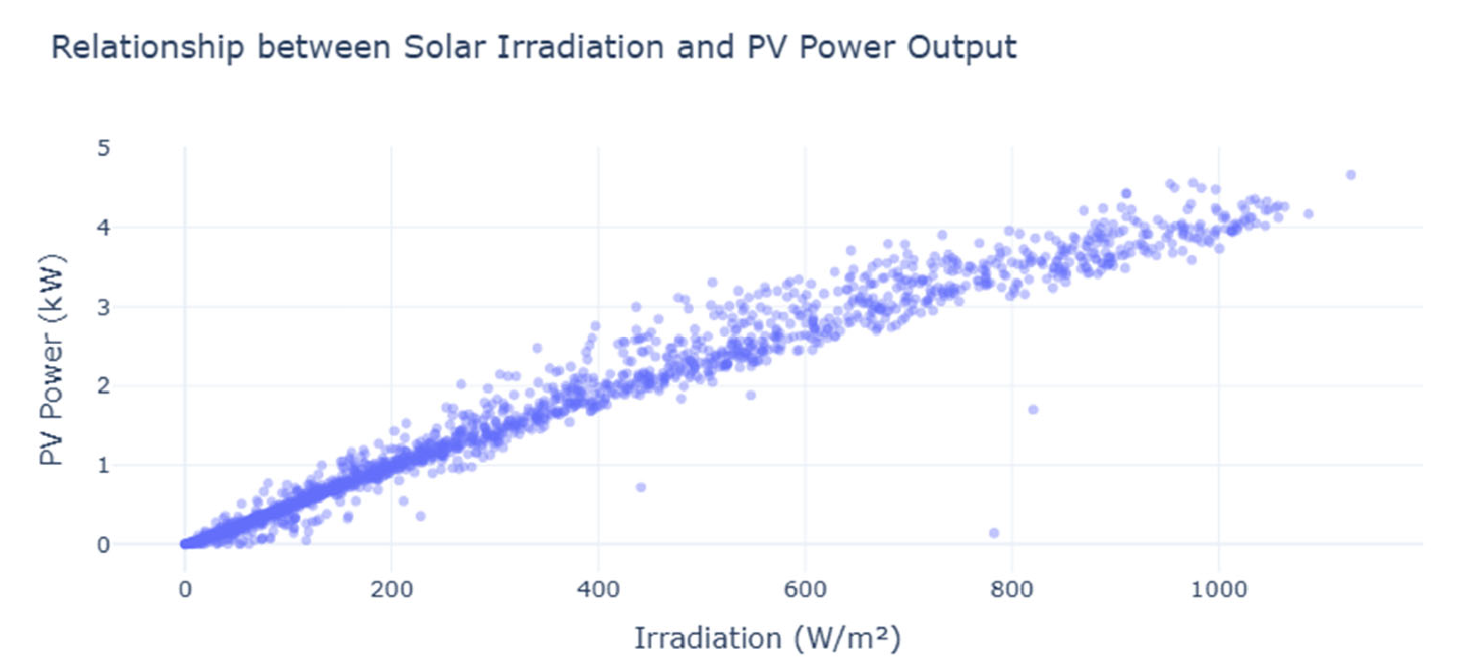For each time step, the dataset included measured PV power output (kW) and global solar irradiation (W/m²). While additional meteorological variables such as ambient temperature and wind speed were available in the original data source, preliminary correlation analysis confirmed that irradiation and historical power output dominated the hour-ahead forecasting performance for this site. The correlation plot is shown in Figure 2. Consequently, this study focused only on these two features in order to maintain methodological clarity and avoid unnecessary feature redundancy. In all forecasting models investigated, global irradiance and lagged PV power were jointly used as input features. Irradiance therefore acted as the primary exogenous driver, while historical power captured short-term persistence and plant-specific dynamics.

Although additional meteorological variables such as ambient temperature, cloud cover, and numerical weather prediction (NWP) outputs were commonly used in PV forecasting, this study deliberately restricted the input space to historical PV power and global horizontal irradiance. This choice was motivated by both practical and methodological considerations. For hour-ahead horizons, PV power exhibited strong temporal persistence and a dominant dependence on contemporaneous irradiance, while the incremental predictive value of other meteorological variables was shown to be marginal or inconsistent in previous studies. Moreover, short-term NWP products may introduce additional uncertainty and temporal mismatch at such fine resolutions. By limiting the inputs, the present study isolated the effects of model structure and probabilistic calibration, enabling a clearer comparison across forecasting models.

To substantiate the feature selection, Pearson correlation coefficients were also computed over the full five-year dataset. PV power exhibited a very strong linear relationship with global horizontal irradiation (r = 0.974), indicating that irradiation alone explained approximately 95% of the linear variability in power output. In contrast, ambient temperature showed a substantially weaker correlation (r = 0.515), much of which was attributable to its collinearity with irradiation (r = 0.567). These results confirmed that irradiation was the dominant explanatory variable for hour-ahead PV forecasting at this site.

Potential snow-related anomalies were investigated by identifying instances of moderate-to-high irradiation (irradiation > 400 W/m²) combined with near-zero power output. Only a single such event was detected over the entire five-year period, indicating that snow-induced deviations were extremely rare in this dataset and did not materially influence model training or probabilistic calibration.

The target variable in this study was the measured AC PV power output rather than a normalized or irradiance-adjusted quantity. Although PV power could be influenced by hardware-specific factors such as inverter efficiency, maximum power point tracking (MPPT) behavior, and long-term module degradation, these effects were deterministic and relatively stable over time for a given installation. From an operational perspective, the variable of practical interest for grid integration and intraday market participation was the actual delivered power. Consequently, modeling the full system response including hardware characteristics provided a realistic evaluation of forecasting performance under real operating conditions.

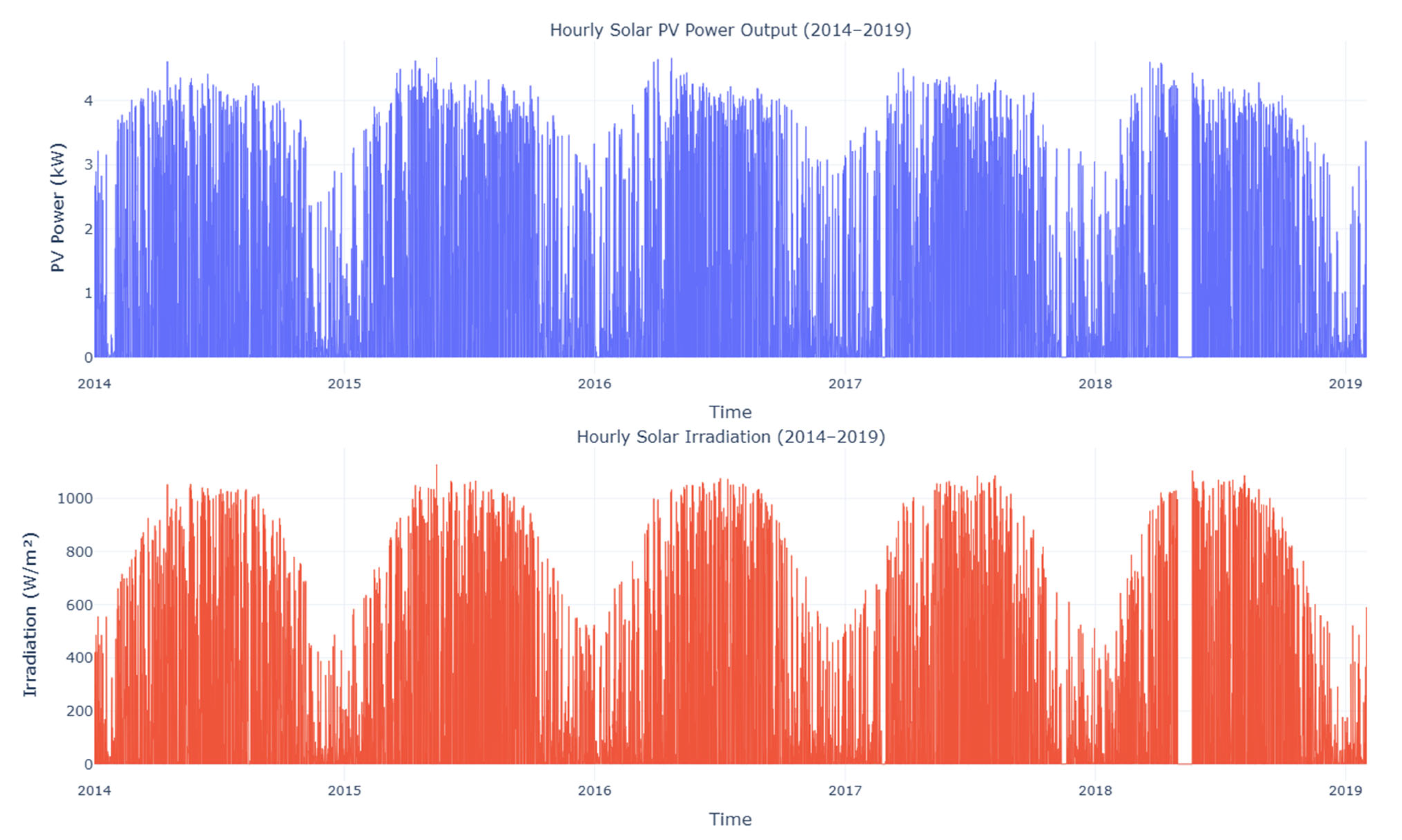
Figure 3 illustrates the temporal evolution of the hourly PV power output over the full five-year period. The strong diurnal and seasonal patterns characteristic of solar generation are clearly visible, with extended nighttime periods of zero output and pronounced seasonal amplitude variations. These structural properties of the data played a critical role in both deterministic forecasting performance and probabilistic calibration, particularly for adaptive methods such as conformal inference. It has to be mentioned that the solar panel, along with the irradiation meter, were taken out for maintenance from 1 May to 22 May 2018. That data gap is visible and was not removed for any model, allowing for comparison of performance under the same conditions for all.

Based on the analysed dataset, photovoltaic power output exhibited pronounced intermittency driven by the deterministic diurnal cycle of solar irradiation. During daylight hours, defined as periods with non-zero irradiation, the mean PV power output was 0.68 kW, indicating that most operating conditions corresponded to partial-load generation rather than sustained peak production. The maximum observed PV power reached 4.67 kW, which was consistent with the nominal capacity of the installation, while the maximum recorded irradiation was 1127.8 W/m², representing clear-sky conditions.

These characteristics highlight several challenges inherent to hour-ahead PV forecasting. First, the high fraction of zero-output periods introduces sharp regime transitions between nighttime and daytime operation, which can bias both deterministic error metrics and probabilistic calibration if not handled explicitly. Second, the dominance of sub-maximal operating points implies that forecasting performance is largely determined by the ability to capture moderate irradiation-driven variability rather than rare peak events. These properties motivate the use of forecasting models that can accommodate short-term dependencies while remaining robust to structural discontinuities.

4.2. Data Preprocessing

Prior to model training, the raw PV power and solar irradiation time series were preprocessed to ensure numerical stability, prevent data leakage, and enable a fair comparison across forecasting models with fundamentally different structures. All preprocessing steps were applied consistently across models and relied exclusively on information available to the forecast origin.

For linear and regression-based models, including persistence, autoregressive models with exogenous inputs, ridge regression, and the DLinear baseline, a supervised learning representation was constructed using lagged observations of PV power and solar irradiation. Specifically, the input feature vector at time t was defined according to (18):

$${\mathsf{\varphi }}_t={\left[P_{t-1},P_{t-2},I_{t-1}, I_{t-2}\right]}^{\mathrm{\top }}$$

(18)

where P and I denote the power and irradiation values. The target value was the power P_t at time step t and the features were lagged values, as shown in (18).

For sequence-based models, namely, the vanilla LSTM, the same lagged information was reformulated using a sliding window approach, as already described in [22]. Input sequences of fixed length L = 2 was constructed, where each sample consisted of a sequence of past observations of PV power and irradiation. This representation preserved temporal ordering while ensuring that no future information was used during model training or inference.

To ensure numerical stability and facilitate fair comparison across forecasting models with different optimization dynamics, all input features were standardized using z-score normalization. For a given variable x, the normalized value x* was computed according to (19):

$$x^{\ast }={\displaystyle \frac{x-\mathsf{\mu }}{\mathsf{\sigma }}}$$

(19)

where μ and σ denote the mean and standard deviation of the variable, respectively.

Normalization parameters were computed exclusively on the training dataset to prevent information leakage and subsequently applied unchanged to the test set. Input features (lagged PV power and solar irradiation) and the target variable (PV power) were normalized independently using separate scaling parameters. For models trained on normalized targets, inverse transformation was applied to the predicted values prior to performance evaluation, ensuring that all reported results were expressed in the original physical units.

This normalization strategy was applied consistently across all forecasting models considered in this study, including linear regression, ridge regression, DLinear, and LSTM, thereby ensuring that observed performance differences were attributable to model structure rather than scaling effects.

To ensure an evaluation consistent with operational hour-ahead forecasting settings, the dataset was partitioned using a strictly chronological split. No rolling or expanding window evaluation strategy was employed. Instead, the first 80% of the available time series data (January 2014 to approximately mid-2018) was used for model training, while the remaining 20% (mid-2018 to January 2019) was reserved exclusively for out-of-sample testing.

This fixed temporal partitioning prevented information leakage from future observations and ensured that all forecasting models were evaluated under identical conditions. For sequence-based models such as the LSTM and DLinear, supervised learning samples were constructed using a fixed-length sliding window over past observations. This procedure was applied after the chronological data split and served solely to generate input–output pairs required by these architectures. Importantly, this sliding window mechanism did not constitute a rolling or expanding window evaluation, as model parameters were trained once on the fixed training subset and evaluated on a separate, unseen test subset without model updates.

This sliding window procedure as shown in Algorithm 1 was used exclusively to construct supervised learning samples for sequence-based models and did not imply a rolling or expanding window evaluation. Model training was performed once on the fixed training subset, and all generated windows remained confined within their respective training or test partitions.

Algorithm 1 Supervised sliding window construction for sequence models

Input: Time series of explanatory variables $X=\{x_t{\}}_{t=1}^T$ Target variable $y=\{y_t{\}}_{t=1}^T$ Window length C Output: Set of input–output training samples $\left\{\right(X^{\left(\mathit{i}\right)},y^{\left(i\right)}\left)\right\}$ Initialize empty sets $\mathcal{X}$ and $\mathcal{Y}$ to store input sequences and corresponding targets For each time index $t=\mathrm{1,2},\dots ,T-C+1$ Construct an input sequence $$X^{\left(t\right)}=\left[x_t,x_{t+1},\dots ,x_{t+C-1}\right]$$ Assign the corresponding target value $$y^{\left(t\right)}=y_{t+C-1}$$ Append $X^{\left(t\right)}$ to $\mathcal{X}$ and $y^{\left(t\right)}$ to $\mathcal{Y}$ Repeat until all feasible sequences of length C have been generated Return the constructed input–output pairs $(\mathcal{X},\mathcal{Y})$

4.3. Hyperparameter Selection

To ensure a fair and transparent comparison across forecasting models, all hyperparameters were fixed a priori and kept constant throughout the experiments. No automated hyperparameter optimization was performed, as the objective of this study was to assess the impact of model complexity under comparable and reproducible settings rather than to maximize individual model performance through extensive tuning.

For the linear regression-based models, the ARX model was configured with a lag order of one for both the target variable and the exogenous input, i.e., p = 1 and q = 1. This choice reflected the very short temporal dependencies typical of hour-ahead PV forecasting and was consistent with operational forecasting practices. Ridge regression employed an ℓ2 regularization parameter of λ = 1.0, which was found to provide numerical stability without materially altering predictive performance relative to the unregularized ARX formulation.

The DLinear model was implemented as a single linear mapping applied to the flattened sliding window input, without additional decomposition or attention mechanisms. It was trained using the Adam optimizer with a learning rate of 10^{− 3}, a batch size of 32, and 20 training epochs.

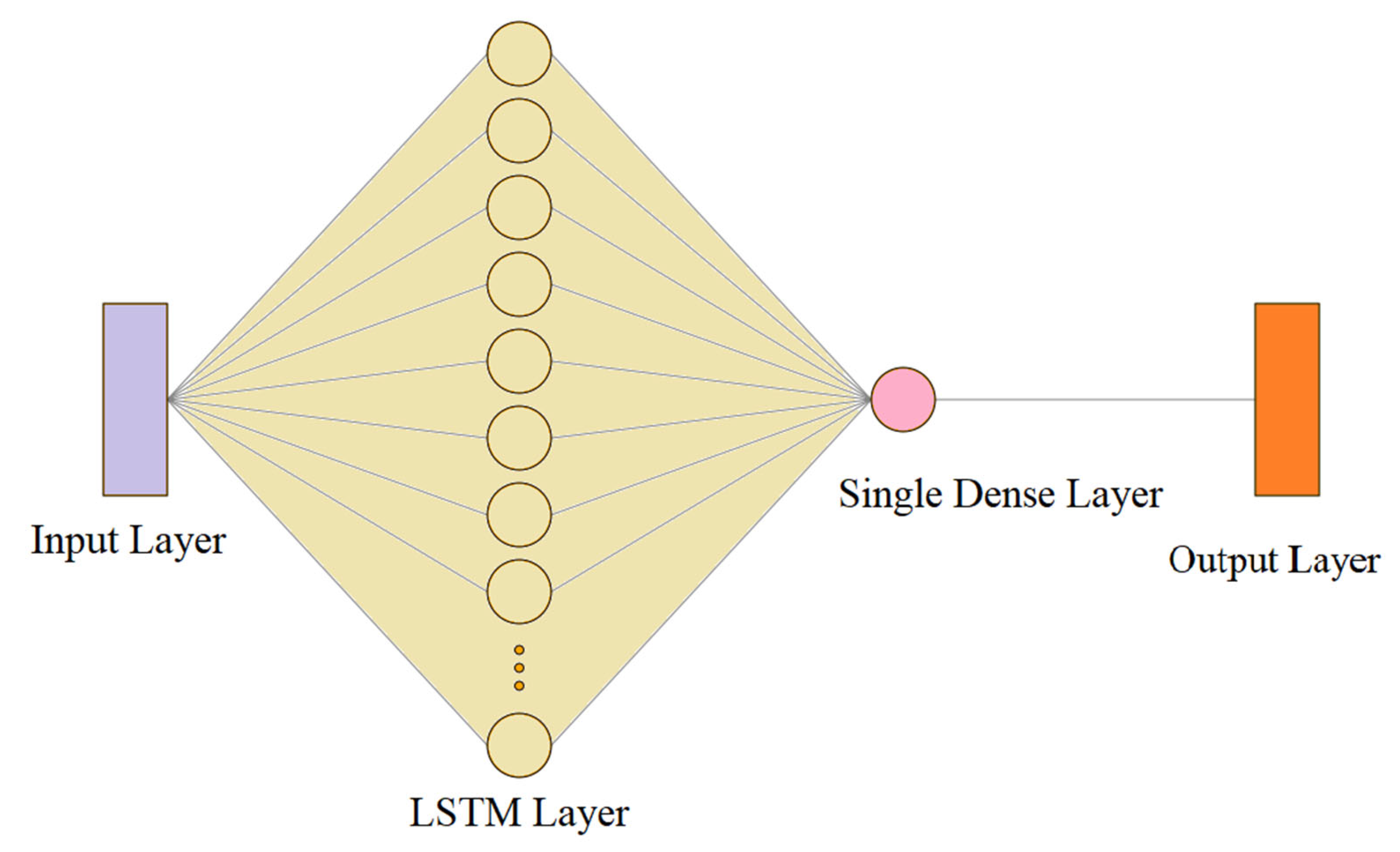
The vanilla LSTM model consisted of a single recurrent layer with five hidden units, followed by a fully connected output layer. The model was trained using the Adam optimizer with a learning rate of 10⁻³, a batch size of 24, and 20 training epochs. Rectified Linear Unit (ReLU) activation was used in the LSTM cell, following the implementation adopted in the experimental codebase.

All neural network models were trained using mean squared error as the loss function. Early stopping was not employed, as training convergence was observed well within the specified number of epochs. Identical normalization and data partitioning procedures were applied across all models to ensure consistency.

5. Evaluation Metrics

To comprehensively assess the performance of the proposed forecasting models, both deterministic and probabilistic evaluation metrics were employed. Deterministic metrics quantified point forecast accuracy, while probabilistic metrics assessed the reliability, sharpness, and overall quality of the associated prediction intervals. This dual evaluation framework ensured that improvements in point accuracy were not achieved at the expense of uncertainty miscalibration.

5.1. Deterministic Evaluation Metrics

Deterministic performance was evaluated using the RMSE and MAE, which are widely adopted in short-term photovoltaic power forecasting due to their interpretability and sensitivity to different error characteristics. The RMSE was defined according to (20):

$$\mathrm{RMSE}=\sqrt{{\displaystyle \frac{1}{N}}{\sum }_{t=1}^N{\left(P_t-\widehat{P_t}\right)}^2}$$

(20)

where P_t denotes the PV power and $\widehat{P_t}$ is the corresponding forecast. N is the number of samples. RMSE penalized large forecast errors more strongly and was therefore sensitive to extreme deviations [26]. The MAE was defined according to (21):

$$\mathrm{MAE}={\displaystyle \frac{1}{N}}{\sum }_{t=1}^N\left|P_t-\widehat{P_t}\right|$$

(21)

MAE provided a robust measure of average absolute forecast deviation and was less influenced by outliers than RMSE [27]. Together, RMSE and MAE provided complementary insight into deterministic forecasting performance.

5.2. Probabilistic Evaluation Metrics

Probabilistic performance was assessed using prediction interval-based metrics that jointly evaluated forecast reliability and sharpness. Let $\left[{\underset{\_}{P}}_t,{\overline{P}}_t\right]$ denote the lower and upper bounds of the prediction interval at time t, constructed for a nominal coverage level 1 − α. The Prediction Interval Coverage Probability (PICP) measured the empirical coverage of the prediction intervals and was defined according to (22):

$$\mathrm{PICP}={\displaystyle \frac{1}{N}}{\sum }_{t=1}^{N}I\left\{P_t\in \left[{\underset{\_}{P}}_t,{\overline{P}}_t\right]\right\}$$

(22)

where I(⋅) denotes the indicator function. Ideally, PICP should be close to the nominal confidence level 1 − α, indicating well-calibrated uncertainty estimates [28]. The Mean Prediction Interval Width (MPIW) quantified the average sharpness of the prediction intervals and was defined according to (23):

$$\mathrm{MPIW}={\displaystyle \frac{1}{N}}{\sum }_{t=1}^N\left({\overline{P}}_t-{\underset{\_}{P}}_t\right)$$

(23)

Smaller MPIW values indicated sharper intervals; however, sharpness needed to be interpreted jointly with coverage, as overly narrow intervals could result in poor calibration [29]. The Winkler score provided a combined measure of interval sharpness and calibration by penalizing both wide intervals and observations falling outside the interval. It was defined according to (24):

$$\mathrm{W}{\mathrm{S}}_{\mathrm{t}}=\left({\overline{P}}_t-{\underset{\_}{P}}_t\right)+{\displaystyle \frac{2}{\mathsf{\alpha }}}\left({\underset{\_}{P}}_t-P_t\right)\hspace{0.17em}I\left(P_t<{\underset{\_}{P}}_t\right)+{\displaystyle \frac{2}{\mathsf{\alpha }}}\left(P_t-{\overline{P}}_t\right)\hspace{0.17em}I\left(P_t>{\overline{P}}_t\right)$$

(24)

The reported Winkler score corresponded to the average of WS_t over all test samples. Lower values indicated better probabilistic performance [30]. The CRPS evaluated the quality of the predictive distribution by measuring the discrepancy between the predicted cumulative distribution function and the empirical observation. For interval-based probabilistic forecasts, CRPS could be approximated according to (25):

$$\mathrm{CRPS}={\displaystyle \frac{1}{N}}{\sum }_{t=1}^N\left[\left({\overline{P}}_t-{\underset{\_}{P}}_t\right)+{\displaystyle \frac{2}{\mathsf{\alpha }}}\left({\underset{\_}{P}}_t-P_t\right)I\{P_t<{\underset{\_}{P}}_t\}+{\displaystyle \frac{2}{\mathsf{\alpha }}}\left(P_t-{\overline{P}}_t\right)I\{P_t>{\overline{P}}_t\}\right]$$

(25)

CRPS provided a strictly proper scoring rule that jointly accounted for calibration and sharpness, with lower values indicating superior probabilistic forecasts [31].

6. Results

6.1. Deterministic Performance

The deterministic forecasting performance of all considered models is summarized in

Table 1. Deterministic forecast performance.

Model	RMSE (kW)	RMSE (% of 5.13 kW)	RMSE Improvement vs. Persistence (%)	MAE (kW)	MAE (% of 5.13 kW)
Persistence	0.452	8.81	0.00	0.222	4.33
ARX	0.383	7.47	15.27	0.212	4.13
Ridge	0.383	7.47	15.27	0.212	4.13
DLinear	0.384	7.49	15.04	0.198	3.86
LSTM	0.336	6.55	25.66	0.164	3.20

using RMSE and MAE. Errors are reported both in absolute terms and relative to the nominal 5 kW capacity of the photovoltaic system to facilitate practical interpretation.

The persistence model provided a strong baseline, achieving an RMSE of 0.45 kW (8.81%), reflecting the high temporal continuity of PV power at the hour-ahead horizon. Linear regression-based models, including ARX and ridge regression, yielded a clear improvement over persistence, reducing the RMSE to approximately 0.38 kW (7.47%) and the MAE to 0.21 kW (4.13%). The near-identical performance of ARX and ridge regression indicated that explicit regularization did not provide additional benefit under the selected lag structure and data conditions.

The DLinear model achieved comparable RMSE to the linear regression models while exhibiting a slightly lower MAE (0.20 kW, 3.86%), suggesting marginal improvements in average absolute error but limited gains in overall error dispersion. The vanilla LSTM achieved the best deterministic performance among the evaluated models, with an RMSE of 0.34 kW (6.55%) and an MAE of 0.16 kW (3.2%). However, the absolute improvement relative to linear models remained modest, corresponding to an RMSE reduction of approximately 0.05 kW, or 1% of system capacity.

To facilitate comparison across models, Table 1 also reports the relative improvement of each method with respect to the persistence benchmark. Using persistence as a reference, linear models reduced RMSE by approximately 15%, while DLinear achieved a 15.0% reduction. The LSTM provided the largest gain, reducing RMSE by 25.7% and MAE by 26.1% relative to persistence. When normalized by the installed STC capacity of 5.13 kWp, the LSTM achieved an RMSE of 6.55% of rated power, compared to 8.81% for persistence.

In order to verify whether the choice of PV power as the direct forecasting target influenced the conclusions, an additional two-step baseline was evaluated. In this formulation, the LSTM model was trained to predict hour-ahead global irradiance, after which a linear irradiance-to-power mapping (estimated exclusively on the training set) was applied to obtain power forecasts. The resulting indirect power forecast achieved an RMSE of 0.316 kW (6.16% of the 5.13 kWp installed capacity) and an MAE of 0.171 kW. Compared to the direct LSTM power forecast (RMSE 0.336 kW, 6.55% of capacity), the difference amounted to only 0.020 kW, corresponding to less than 0.4% of rated capacity. This confirmed that the marginal performance differences observed between models were not driven by the choice of target formulation but reflected the intrinsic predictability limits at the hour-ahead horizon.

Overall, these results indicate that while deep learning can provide incremental improvements in point forecasting accuracy, the majority of predictive performance at the hour-ahead horizon was already captured by simple linear models leveraging short-term lagged information and exogenous irradiation inputs.

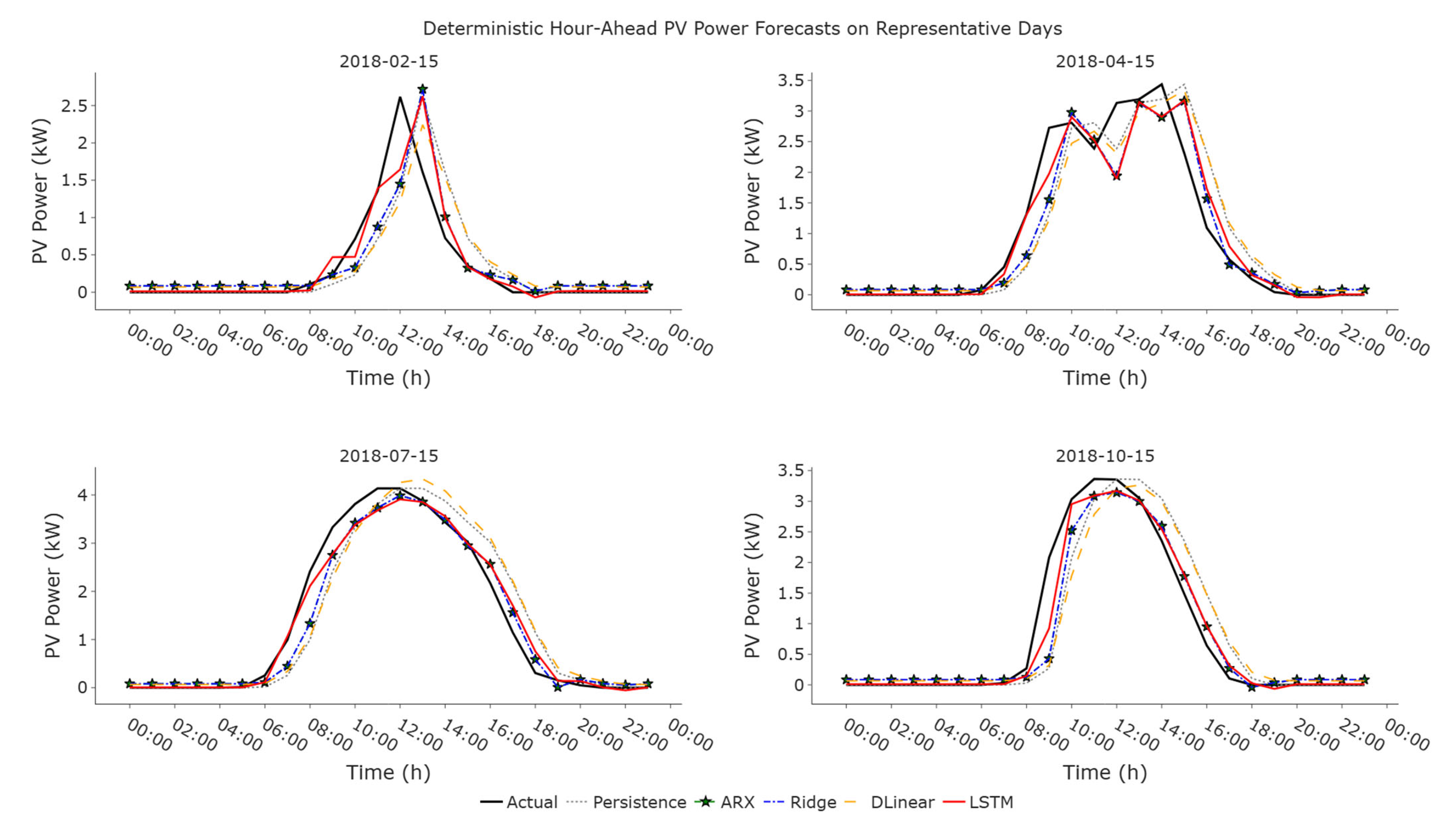
Figure 4 illustrates the hour-ahead deterministic PV power forecasts produced by the considered models for four representative days selected from different seasons. The chosen days captured a range of operating conditions, including winter and autumn periods characterized by shorter daylight hours and lower peak generation, as well as spring and summer days exhibiting longer production windows and higher irradiance levels.

Across all seasons, the persistence model provided a reasonable baseline by reproducing the general diurnal shape of PV generation but systematically exhibited temporal lag during ramp-up and ramp-down periods, particularly around sunrise and sunset. This behavior was most pronounced during the winter day (15 February 2018), where rapid changes in PV output led to underestimation during the morning ramp and delayed response during the afternoon decline. A similar behaviour can be noticed during 15 October 2018 when all models seem to be operating on a consistent lag except the LSTM model at some instances where it captures the curve more accurately at 10:00 a.m. and from 14:00 to 18:00 p.m.

The linear regression-based models (ARX and Ridge) demonstrated consistently improved tracking of the diurnal profile compared to persistence. These models more accurately captured the timing and magnitude of the midday peak, especially during the spring day (15 April 2018), reflecting the strong dependence of hour-ahead PV output on recent power observations and irradiance dynamics. Differences between ARX and Ridge were visually negligible across all days, indicating limited benefit from regularization under the selected lag structure and data regime. 15 July 2018 exhibits similar performance with the exception during mid-day where volatility was introduced due to changing weather conditions. During this disruption the LSTM model once again provided better forecasts compared to the rest.

The DLinear model exhibited behavior similar to the linear baselines, with slightly smoother responses during transition periods but no systematic improvement in peak or ramp tracking. In several cases, particularly during the summer day, DLinear tended to marginally underpredict the peak output, consistent with its weaker deterministic performance observed in the quantitative evaluation.

The LSTM model provided the closest alignment with the observed PV power across all four days, particularly during periods of rapid intra-day variation. Improvements were most evident during the morning ramp-up and around the peak generation window, where the LSTM better captured short-term nonlinearities and temporal dependencies. However, the magnitude of these improvements remained modest, and the overall diurnal structure was already well captured by the simpler linear models.

6.2. Probabilistic Performance

Table 2. Probabilistic forecast performance.

Model	PICP (%)	MPIW (kW)	Winkler Score (kW)	CRPS (kW)
Persistence	90.94	1.634	2.353	0.927
ARX	91.06	1.165	1.995	0.677
Ridge	91.06	1.166	1.995	0.677
DLinear	90.78	1.659	2.400	0.943
LSTM	91.43	1.079	1.747	0.620

reports the probabilistic forecasting performance of all considered models after applying adaptive conformal inference with a daily miscoverage reset at a nominal confidence level of 90%. Across all models, the achieved prediction interval coverage probabilities (PICP) were close to the target value, ranging from 0.908 to 0.914. This indicated that the proposed calibration framework successfully enforced reliable coverage, irrespective of the underlying deterministic forecasting model.

While coverage levels were nearly identical, differences emerged in terms of interval sharpness and overall probabilistic accuracy. The LSTM model yielded the narrowest prediction intervals, with an average MPIW of 1.08 kW, and achieved the lowest Winkler score (1.75 kW) and CRPS (0.62 kW). These results suggest that the LSTM was able to produce slightly sharper and more informative uncertainty estimates, particularly during periods of rapid intra-day variability.

Linear regression-based models (ARX and Ridge) demonstrated highly competitive probabilistic performance. Both models achieved virtually identical coverage and interval quality, with MPIW values of approximately 1.17 kW and CRPS values of around 0.68 kW. The negligible difference between ARX and Ridge confirmed that ℓ₂ regularization provided limited benefit under the selected lag structure and data regime. Importantly, the probabilistic performance of these simple linear models remained close to that of the LSTM, despite their significantly lower model complexity and computational cost.

In contrast, the DLinear and persistence baselines required substantially wider prediction intervals to maintain nominal coverage, resulting in higher Winkler scores and CRPS values. DLinear exhibited the weakest probabilistic performance among the learning-based models, even under conformal calibration, while persistence remained limited by its inability to adapt to rapid changes in PV output.

Overall, the results demonstrate that once uncertainty is explicitly accounted for through a unified, model-agnostic calibration framework, the performance gap between simple linear models and more complex deep learning architectures at the hour-ahead horizon is considerably reduced. This highlights the importance of reliable uncertainty quantification over marginal improvements in point forecast accuracy when evaluating short-term PV forecasting models.

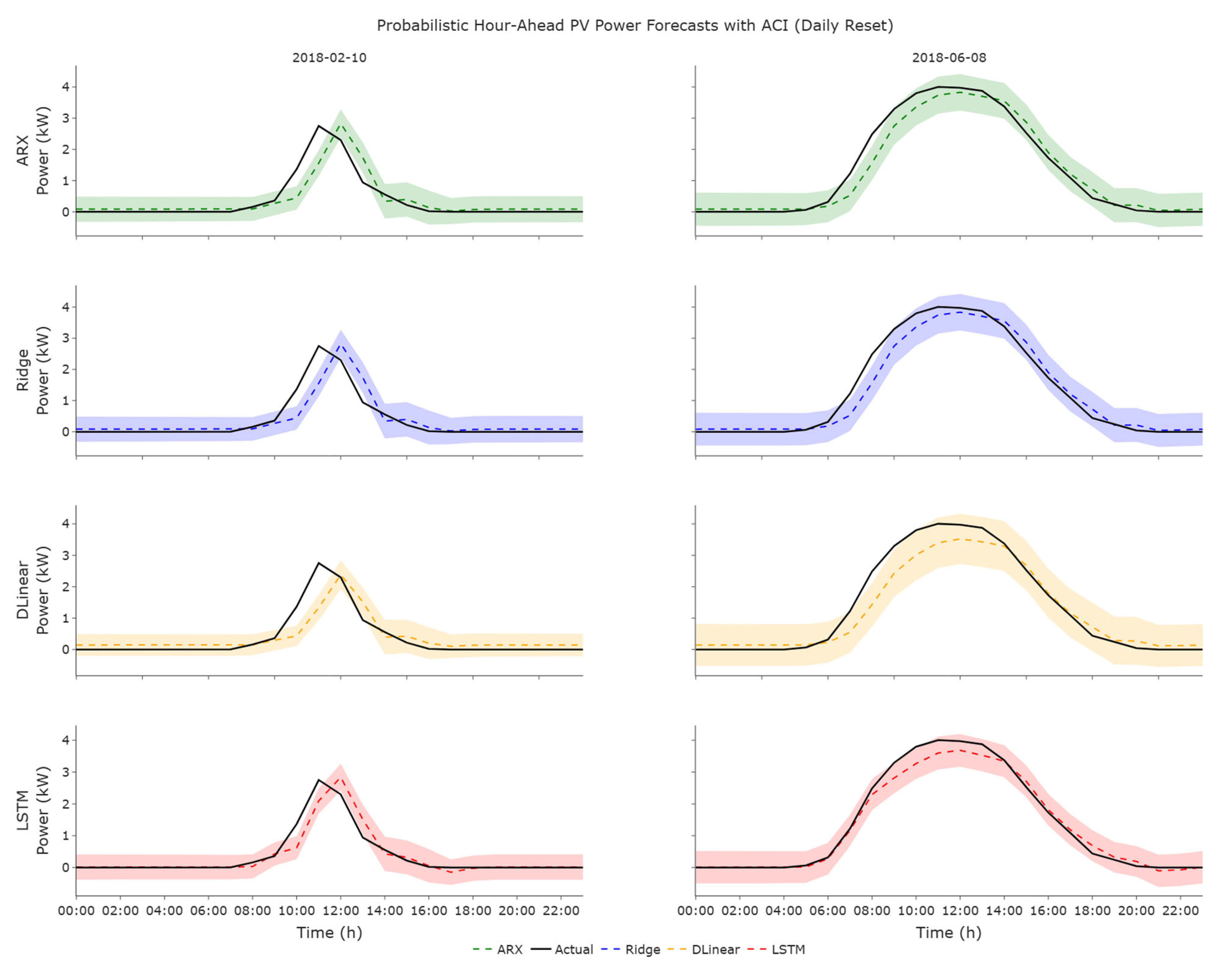
Figure 5 illustrates probabilistic hour-ahead PV power forecasts obtained using ACI with a daily miscoverage reset for two representative test days: a winter day (left column) and a summer day (right column). Each row corresponds to a different forecasting model: ARX, Ridge, DLinear, and LSTM, allowing for a direct visual comparison of model-specific uncertainty behavior under identical seasonal conditions. The solid black line denotes the observed PV power output, dashed colored lines represent the median (point) forecasts produced by each model, and the shaded regions indicate the calibrated prediction intervals generated by the ACI framework.

For the winter day, all models failed to capture the sharp midday production peak characteristic of clear-sky conditions, with prediction intervals widening around the ramp-up and ramp-down periods where forecast uncertainty was highest. In contrast, the summer day exhibited a smoother and broader diurnal profile with extended high-production hours, leading to narrow and stable prediction intervals across models. This seasonal contrast highlights the ability of the proposed probabilistic framework to adapt the interval width to both the magnitude and variability of PV generation.

Despite noticeable differences in deterministic tracking accuracy, particularly during rapid transitions and peak production, the resulting prediction intervals across ARX, Ridge, DLinear, and LSTM remained broadly comparable in terms of coverage and temporal evolution. In particular, the linear models (ARX and Ridge) and the deep learning model (LSTM) produced similarly calibrated uncertainty bands after conformal adjustment, while DLinear exhibited slightly wider intervals during high-variability periods. The LSTM performed slightly better than all, but at the expense of computational cost. These observations visually corroborate the quantitative results reported in Table 2, demonstrating that once probabilistic calibration is applied in a model-agnostic manner, differences in uncertainty representation between simple and complex forecasting models at the hour-ahead horizon are substantially reduced.

To quantitatively assess computational efficiency, wall-clock training and inference times were measured for all models under identical hardware and data partitioning conditions, as noted in

Table 3. Computational demand of the investigated models.

Model	Training Time (s)	Inference Time (s)	Total Time (s)
Persistence	0.00023	0.00000	0.00023
Linear Regression	0.03016	0.00179	0.03195
Ridge Regression	0.02080	0.00278	0.02358
DLinear	12.74400	0.00984	12.75384
LSTM	83.77249	1.61992	85.39241

. Linear models exhibited extremely low computational cost, with total runtimes below 0.05 s for both linear regression and ridge regression. In contrast, the DLinear model required approximately 12.8 s, while the LSTM required over 85 s due to iterative gradient-based optimization. Notably, despite these substantial differences in computational cost spanning more than three orders of magnitude, all models achieved comparable empirical coverage after adaptive conformal inference calibration. This result highlights that at the hour-ahead horizon, reliable probabilistic forecasting can be achieved without incurring the high computational burden associated with deep learning architectures.

7. Discussion

This study examined whether increased model complexity yields practically meaningful improvements in hour-ahead solar PV power forecasting when uncertainty is evaluated within a unified, model-agnostic probabilistic framework. By jointly analyzing deterministic accuracy and probabilistic reliability across a spectrum of forecasting models, from persistence and linear regression to deep learning models, the results provide several important insights with direct implications for short-term PV forecasting practice.

The forecasting target in this study was measured AC power at the inverter level, which inherently integrates meteorological variability together with plant-level and control-related effects. From an operational perspective, this integrated quantity represents the relevant forecasting variable for grid management and intraday scheduling. While it is true that separating pure irradiance-driven variability from hardware-induced nonlinearities could offer additional physical interpretability, the objective of this benchmarking study was to assess model performance under realistic plant operating conditions. All models were trained and evaluated on the same measured output signal; therefore, hardware-related effects were uniformly embedded across model classes and did not bias comparative conclusions regarding model complexity.

From a deterministic perspective, the results confirm trends widely reported in the literature: more complex models, particularly recurrent neural networks, tend to achieve the lowest point forecast errors. The vanilla LSTM delivered the best RMSE and MAE among the evaluated approaches, outperforming persistence and linear baselines across all tested seasons. However, the absolute magnitude of these improvements was modest. The reduction in RMSE relative to linear models corresponded to approximately 1% of system capacity, indicating that at the hour-ahead horizon, most predictive information was already captured by recent lagged power and irradiance observations. Importantly, the deterministic results alone provide an incomplete picture of forecast usefulness. When probabilistic performance is considered through ACI, the apparent performance gap between simple and complex models narrows substantially. All forecasting models achieved empirical coverage levels close to the nominal 90% target, demonstrating the effectiveness of the proposed model-agnostic calibration framework. This confirms that, once properly calibrated, fundamentally different forecasting paradigms can be made equally reliable in terms of coverage, supporting fair comparison across model classes.

Differences emerged primarily in terms of interval sharpness and overall probabilistic quality. The LSTM produced the narrowest prediction intervals and achieved the lowest Winkler score and CRPS, indicating slightly more informative uncertainty estimates. However, linear models such as ARX and ridge regression exhibited probabilistic performance remarkably close to that of the LSTM, despite their substantially lower computational complexity and training overhead. The near-identical behavior of ARX and ridge regression further suggests that regularization provided limited benefit under the selected lag structure and data regime, reinforcing the conclusion that structural simplicity is not a disadvantage at the hour-ahead horizon.

The DLinear model, while conceptually appealing as an intermediate benchmark between linear regression and deep learning, does not demonstrate consistent advantages in either deterministic or probabilistic performance. Its requirement for wider prediction intervals to maintain nominal coverage indicates weaker inherent predictive stability compared to both classical linear models and the LSTM. Persistence, although competitive as a deterministic baseline, remains fundamentally limited in both point accuracy and probabilistic sharpness due to its inability to adapt to rapid changes in irradiance and PV output.

The visual analysis of representative winter and summer days further reinforces these findings. Seasonal differences dominated forecast uncertainty behavior: winter days with short daylight windows and sharp midday peaks induced wider intervals across all models, while summer days exhibited smoother profiles and more stable uncertainty estimates. Crucially, after conformal calibration, the temporal evolution of prediction intervals was broadly similar across models, highlighting that uncertainty behavior is driven more by data characteristics and calibration strategy than by model architecture itself.

Although snow accumulation can temporarily reduce PV output independently of irradiation, such events were virtually absent in the present dataset. From a probabilistic standpoint, the adaptive conformal inference framework naturally accommodates rare anomalies through localized increases in conformity scores, resulting in temporary interval widening without systematic degradation of calibration or sharpness. Therefore, the exclusion of additional snow-related predictors does not compromise the robustness of the proposed methodology for the analyzed horizon.

The use of only PV power and global irradiance as inputs raises the question of how additional explanatory variables might affect probabilistic forecast quality, particularly prediction interval sharpness. In principle, informative exogenous variables could reduce residual uncertainty and lead to narrower conformal intervals. However, for hour-ahead PV forecasting, additional meteorological variables such as temperature or cloudiness often exhibit weak incremental predictive power once irradiance is known, while short-horizon NWP inputs may themselves be noisy or biased. Since adaptive conformal inference adjusts interval widths based on recent forecast errors, improvements in sharpness are ultimately constrained by the stability and accuracy of the underlying point forecasts. If additional variables do not systematically reduce point forecast errors, their impact on conformal interval sharpness is likely to be limited or even adverse. The results presented here suggest that for very short horizons, robust uncertainty quantification combined with parsimonious models can be more effective than increasing input dimensionality.

Taken together, these results suggest that for hour-ahead PV forecasting, the choice of probabilistic calibration framework may be more consequential than the choice of deterministic forecasting model. While deep learning models offer incremental gains in both point accuracy and uncertainty sharpness, well-designed linear models combined with robust, model-agnostic probabilistic calibration can achieve nearly equivalent decision-relevant performance. This finding has important practical implications, particularly for operational settings where computational efficiency, interpretability, and ease of deployment are critical.

It is important to emphasize that the forecasting target considered in this study is inverter-level AC power, which inherently integrates meteorological variability together with plant- and control-related nonlinearities. The conclusions drawn regarding model complexity therefore apply to operational power forecasting under real system conditions. They should not be interpreted as general statements about the relative value of complex models for pure irradiance prediction or physically disaggregated modeling tasks.

Future Research Directions

Several directions for future work emerge from this study. First, extending the proposed framework to longer forecasting horizons (e.g., multi-hour or day-ahead) would help determine whether the relative importance of model complexity increases as temporal dependencies become more pronounced. Second, incorporating additional exogenous information such as sky imagery, numerical weather prediction outputs, or satellite-based irradiance estimates could further clarify the interaction between model complexity and information richness within a probabilistic setting.

From a methodological standpoint, future research could explore alternative conformal strategies, including locally adaptive or regime-aware calibration schemes that explicitly distinguish between clear-sky and cloudy conditions. Additionally, integrating the probabilistic forecasts into downstream decision-making tasks such as reserve sizing, intraday trading, or microgrid energy management would enable direct quantification of economic and operational benefits. Also, the integration of richer meteorological information, including temperature, cloud indices, and high-resolution NWP forecasts, within the same conformal framework will be investigated. A systematic analysis of how different classes of exogenous variables influence both point accuracy and conformal interval sharpness across multiple forecasting horizons will be particularly valuable, especially for intraday and day-ahead PV forecasting applications.

Finally, while this study focused on a single PV installation, applying the proposed framework across diverse geographical locations, climates, and system scales would provide further evidence of its generalizability. Such extensions would contribute to establishing model-agnostic probabilistic calibration as a standard evaluation and deployment paradigm for short-term renewable energy forecasting.

8. Conclusions

This paper investigated deterministic and probabilistic hour-ahead solar photovoltaic power forecasting using models of varying complexity within a unified, model-agnostic uncertainty quantification framework. The primary objective was to assess whether increased model complexity leads to practically meaningful improvements at very short forecasting horizons when forecast uncertainty is explicitly considered.

Deterministic results show that the vanilla LSTM achieved the lowest point forecast errors, with an RMSE of 0.336 kW (6.55% of rated capacity) and an MAE of 0.164 kW (3.20%), outperforming persistence and linear models. Linear regression-based approaches (ARX and ridge regression) achieved RMSE values of approximately 0.38 kW (7.47%), indicating that a large fraction of predictive skill at the hour-ahead horizon was already captured by simple lagged power and irradiance information. The DLinear model did not provide consistent improvements over classical linear baselines.

When probabilistic performance was evaluated using ACI with a PV-specific daily miscoverage reset, all models achieved empirical coverage close to the nominal 90% level, with PICP values ranging from 90.8% to 91.4%. Differences between models were primarily reflected in interval sharpness rather than coverage. The LSTM produced the narrowest prediction intervals (MPIW = 1.08 kW) and the lowest CRPS (0.62 kW), while linear models exhibited only slightly wider intervals (MPIW ≈ 1.17 kW) and comparable CRPS values (≈0.68 kW). These results demonstrate that after probabilistic calibration, the performance gap between simple linear models and deep learning architectures is substantially reduced.

A key practical finding concerns computational efficiency. Linear models required total runtimes below 0.05 s, compared to 12.8 s for DLinear and over 85 s for the LSTM under identical experimental conditions. Despite these differences spanning more than three orders of magnitude, all models achieved similar probabilistic reliability after conformal calibration. This highlights that for hour-ahead PV forecasting, reliable uncertainty quantification can often be achieved without incurring the high computational cost associated with deep learning models.

Overall, the results indicate that the probabilistic calibration strategy is more influential than deterministic model complexity for hour-ahead PV forecasting. While deep learning models provide incremental gains in point accuracy and interval sharpness, simple and interpretable linear models combined with robust, model-agnostic uncertainty quantification offer competitive, decision-relevant performance at a fraction of the computational cost.