Research on Mechanism-Based Modeling and Simulation of Heavy-Duty Industrial Gas Turbines

Abstract

This study investigates mechanism-based modeling and simulation of a single-shaft heavy-duty industrial gas turbine. Taking the PG9171E gas turbine as the case study, component-level steady-state and dynamic models are developed. The steady-state model is established using the constant mass flow (CMF) method. For dynamic modeling, both the CMF approach and the inter-component volume (ICV) approach are implemented to enable a comparative assessment of the two methods. On the basis of the steady-state model, an improved Dung Beetle Optimization (DBO) algorithm is proposed to perform model correction using measured operational data from the gas turbine. After model correction, the maximum relative error between the simulated results and the measured operating data is reduced to 1.01 × 10⁻⁵%. Following high-accuracy model correction, sensitivity analysis and a comparative dynamic study are conducted for the two dynamic modeling approaches. The results indicate that the most influential sensitivity parameter is the rotor rotational inertia, followed by the virtual volume of the combustor. Moreover, the primary discrepancy between the ICV and CMF approaches arises from differences in the operating trajectories on component characteristic maps. The ICV-based model exhibits a pronounced response lag; however, it requires less computational time than the CMF-based model, making it more suitable for rapid engineering simulation and practical applications.

1. Introduction

As the core power equipment in the fields of energy supply, ship power, and industrial drive, the operational stability, efficiency, and reliability of heavy-duty industrial gas turbines directly determine the overall performance of related systems. Compared with aeroengines, heavy-duty industrial gas turbines feature long-term continuous operation, a wide operating condition adjustment range, and strong coupling between components and control systems, resulting in extremely complex dynamic response and performance degradation mechanisms. To effectively shorten the development cycle of gas turbines, reduce the cost of physical tests, and provide reliable guidance for operating condition adjustment and fault early warning in actual operation, it is of great significance to carry out research on the mechanism-based modeling and simulation of heavy-duty industrial gas turbines.

The mechanistic modeling method of gas turbines has a long history. Back in the 1960s, McKinney et al. [1,2] researched turbofan engine aerothermodynamic modeling methods. Then, Sellers J.F. et al. [3] developed the well-known DYNGEN program for steady-state and dynamic calculations of aeroengines. At present, there are usually two methods for establishing gas turbine mechanism models: one is the inter-component volume (ICV) method, and the other is the constant mass flow (CMF) method. Hashmi et al. [4] summarized the dynamic modeling of variable-geometry industrial gas turbines, pointing out that when dealing with volumes or gas dynamics, CMF is fast but weakens mass accumulation, while ICV has higher accuracy but requires a smaller step size. A common engineering practice is to use CMF for steady-state initialization and ICV for dynamic simulation. Kim et al. [5,6] applied the CMF method to both steady-state and dynamic simulations, and achieved consistent steady-state and dynamic results with manufacturers and PROOSIS while verifying the stability of load-following control. Tsoutsanis et al. [7,8] used CMF for steady-state initialization and then established a modular dynamic model using ICV, which improved dynamic simulation speed while maintaining general accuracy and avoided false dynamics during initialization. Singh R et al. [9] used CMF for steady-state initialization and extended the model into an integrable dynamic state equation using ICV, verifying that the maximum steady-state error is 6% and the dynamic fitting accuracy can reach 88%, supporting subsequent robust control design. Zeng et al. [10] combined an ICV dynamic model with volume state equations and cuckoo search inversion, which is more in line with theoretical laws on degradation identification before and after compressor cleaning and more suitable for maintenance decision-making. Lin et al. [11] built and calibrated a nonlinear dynamic model of a 135 kW micro gas turbine using ICV, and replaced the Newton–Raphson method initialization iteration of CMF with piecewise linear interpolation of steady-state experimental points, enabling control verification in simulation and HIL. Li et al. [12] discussed that the inter-component volume effect can be handled by either the CMF or ICV method, and adopted an improved CMF-based imbalanced mass flow (IMF) approach to capture the volume effect, thereby achieving more realistic transient prediction. Güllü and Aran [13] developed a surge/stall-capable dynamic performance model for a turbojet engine, where the inter-component volume technique enables pre- and post-stall transients under forward and reverse-flow conditions. Goeing et al. [14] compared a constant mass flow (CMF) model with a dynamic approach for a parallel hybrid-electric turbofan and showed that CMF cannot reproduce key aerothermodynamic interdependencies, especially the time-resolved surge-margin behavior. Erario et al. [15] developed and validated a 0-D microturbine transient model using flight data and highlighted practical transient-simulation implementations based on either the ICV method (density changes in plenum volumes) or the CMF iterative method.

In recent years, the mechanism models have been increasingly integrated with data-driven updating and digital-twin concepts. Hu et al. [16] fused a mechanism model with measurement data and introduced an error module to build a gas turbine digital twin, demonstrating improved accuracy and efficiency on LM2500+ operational data for gas-path fault early warning. Guan et al. [17] developed a dual-driven refined model for a heavy-duty gas turbine by integrating thermodynamic modeling with operational-data corrections, which enhanced the consistency between model predictions and plant performance. Zhang et al. [18] proposed a deep multimodel fusion digital-twin approach that integrates machine learning, performance adaptation and component matching, and reported improved simulation consistency with the physical engine during operation. For limited-measurement scenarios, Chi et al. [19] formulated an inverse-problem framework with maximum likelihood parameter estimation to reconstruct compressor characteristics and establish a full-condition model of a 9FA heavy-duty gas turbine, achieving very low relative errors for key compressor discharge parameters.

In these studies, mechanism models serve as the foundational and crucial component. However, discrepancies between generic component maps and the actual operational characteristics of gas turbine components may lead to non-negligible modeling errors. Therefore, prior to applying mechanism models, characteristic correction and performance adaption are necessary to ensure a high degree of model accuracy. Kong et al. [20,21] expressed component characteristics as cubic polynomials and used genetic algorithms to identify coefficients that match test data, thereby obtaining more realistic speed-line characteristics and efficiency distributions. Li et al. [22,23] proposed using genetic algorithms to simultaneously optimize nonlinear scaling coefficients of compressor and turbine maps at multiple operating points, making the component characteristic model consistent with measured data and improving off-design performance prediction under wide operating conditions. Han et al. [24] proposed a reduced-order optimization method (PSO-EKF) combining particle swarm optimization and an extended Kalman filter, which corrects component characteristics by jointly solving prior state estimation and global optimization. Zhang et al. [25] proposed an operational-data-based adaptive improvement method by reverse-calculating normalized characteristic parameters and optimizing tuning factors, thereby improving the accuracy and efficiency of component-map adaptation. Kong et al. [26] introduced a cluster-sampling strategy to select representative field operating points and tuned scaling factors using PSO, reducing the model error from 2.947% to 0.610% on an E-class gas turbine. Jiang et al. [27] proposed a deterministic multi-point calibration method that estimates actual component performance from measurements and synthesizes map scaling factors via interpolation, achieving performance adaptation with low time complexity without heuristic searching. Kim [28] introduced a prediction-focused machine-learning-based adaptation method for both steady-state and transient operation, improving accuracy while reducing computational cost for performance adaptation.

Most of these studies have focused solely on either the CMF method or the ICV method, without performing a thorough comparison of the disparities between them. Consequently, the analysis of the modeling mechanism and comparison of factors influencing model performance are inadequate. During the model calibration process, most studies focus on component characteristics and result in insufficient model accuracy.

Thus, this paper focuses on the mechanism-based modeling and simulation of single-shaft heavy-duty industrial gas turbines. First, thermodynamic component-level modeling ideas are adopted to establish a steady-state model using the CMF method. Second, combined with actual operating data, an improved Dung Beetle Optimization algorithm is employed to correct key model parameters and component maps, reducing the model–plant mismatch. Third, based on the corrected baseline, two dynamic models are established using the CMF method and the ICV method, respectively, and their dynamic simulation characteristics are compared under consistent boundary conditions to support subsequent dynamic characteristic analysis and engineering applications.

2. Mechanism-Based Modeling of Gas Turbines

2.1. Mathematical Model of Gas Turbines

The unit under study is the PG9171E single-shaft heavy-duty industrial gas turbine manufactured by General Electric (GE, Boston, MA, USA). As a major variant of GE’s 9E series, PG9171E is widely used in power generation applications. PG9171E mainly consists of a 17-stage axial-flow compressor, a combustor, a three-stage gas turbine, and an exhaust system, without a free power turbine. Shaft power is delivered to the load through a single rotor. A schematic of the model structure is shown in Figure 1, and the definition of each station number is provided in

Table 1. Definition of each section of the gas turbine.

Section	Number	Section	Number
Inlet of air intake duct	1	Outlet of combustor	4
Inlet of compressor	2	Inlet of gas turbine	41
Bleed air at the 16th stage of the compressor	24	Outlet of gas turbine	42
Outlet of compressor	3	Inlet of exhaust diffuser	6
Inlet of combustor	31	Outlet of exhaust diffuser	7

. In the following text, these numbers are further used as subscripts to denote the parameters at different cross-sections of the gas turbine.

Table 2. Key specifications and ratings of PG9171E.

Category	Key Parameters	ISO-Rated Values	Baseline Values	Unit
Basic Unit Information	Rated Speed	3000	3000	rpm
	Frequency	50	50	Hz
	Fuel Type	Natural Gas/Light Diesel Oil	Natural Gas	--
Core Performance	Rated Output Power (Natural Gas)	123.0	120.0	MW
	Fuel LHV (Natural Gas)	46,670.0	49,736.5	kJ/kg
	Turbine Exhaust Temperature	537	552	°C
Thermodynamic Parameters	Compressor Pressure Ratio	12.6	12.1	--
	Inlet Air Mass Flow Rate	402.8	397.7	kg/s
Thermodynamic Parameters	Turbine Stages	3	3	Stage
	Number of Combustion Chambers	14	14	Unit
Environmental Baseline	Ambient Temperature	15	13	°C
	Atmospheric Pressure	101.325	101.867	kPa

Note: In Table 2, “--” indicates the parameter is dimensionless.

presents the ISO-rated values from the technical specification [29] and the baseline modeling values derived from the operating data. Due to the passage of time, the initial operational data of the studied gas turbine is unavailable. The baseline modeling values are selected from the data collected after a specific water-wash operation of the gas turbine.

Building on the above framework, a steady-state model is first established using the CMF method. Two dynamic models are then developed based on the CMF and ICV methods, respectively, to compare the characteristics of different dynamic modeling approaches.

For the gas turbine simulation model established based on design point data, the input parameters include atmospheric temperature T₀, atmospheric pressure P₀, load power N_gen, natural gas flow rate W_f, and the inlet guide vane angle IGV, and the output parameters include performance parameters such as the flow rate W, total temperature T, and total pressure P of each section.

Due to the very complex working process of gas turbines, it is almost impossible to establish a mathematical model that can fully describe all aspects of their performance and accurately reflect various working states. Therefore, according to actual engineering needs, the following assumptions are made in the gas turbine modeling process:

(1)

The flow of gas in the gas turbine is treated as quasi-one-dimensional flow;

(2)

It is assumed that there is no heat dissipation loss in the components and no heat exchange with the outside world, and the working fluid is regarded as an ideal gas;

(3)

The total pressure recovery coefficient of each flow channel is taken as a constant, ignoring its change with operating conditions.

Currently, there is a substantial amount of research on gas turbine modeling methods, with the primary difference lying in whether to establish an exhaust diffuser (ED) model. Some studies only establish models for the compressor, combustor, and turbine [19,26], and the exhaust pressure of gas turbine is typically approximated as the ambient pressure or prescribed as a constant value. In our research, a more refined ED model is developed. This model centers on the mass flow of ED, with its outlet parameters determined jointly by the coupled effects of gas properties, flow regimes, and geometric characteristics under operating conditions. During the model solving process, the parameters are dynamically updated based on the mass flow continuity equation of the CMF modeling approach or the volume integration of the ICV method. This ED modeling approach aligns more closely with its working mechanism, enabling the acquisition of higher-precision outlet parameters for gas turbines.

The equation for the exhaust diffuser outlet mass flow rate W_g7 is given as follows:

$$W_{\mathrm{g}7}={\displaystyle \frac{P_6{A}_7}{\sqrt{T_6}}}\sqrt{{\displaystyle \frac{2\gamma }{(\gamma -1)R}}{\left({\displaystyle \frac{P_6}{P_0}}\right)}^{-{\displaystyle \frac{2}{\gamma }}}\left[1-{\left({\displaystyle \frac{P_6}{P_0}}\right)}^{{\displaystyle \frac{1-\gamma }{\gamma }}}\right]}$$

(1)

where P₆ is the exhaust diffuser inlet pressure, T₆ is the exhaust diffuser inlet temperature, A₇ is the effective flow area of the exhaust diffuser, γ is the specific heat ratio, and R is the specific gas constant.

The equations for the exhaust diffuser outlet pressure P₇ and temperature T₇ are given as follows:

$$\left\{\begin{array}{l}{P}_7={\sigma }_{\mathrm{ED}}\times P_6\\ T_7=T_6\end{array}\right.$$

(2)

where σ_ED is the total pressure recovery coefficient of the exhaust diffuser.

2.1.1. Steady-State Model of Gas Turbines

When establishing the steady-state model of the gas turbine using the CMF method, the selected initial guess values are the compressor pressure ratio π_C, gas turbine pressure ratio π_G, and rotor speed n. The corresponding three co-operating equations are defined as follows, where ε_i (i = 1, 2, 3) is the residual of the co-operating equation.

The mass flow rate at the inlet of the gas turbine W_g41 is equal to the sum of the mass flow rate at the outlet of the combustor W_g4 and the cooling mass flow rate of the inlet guide vane of the gas turbine W_cool:

$$W_{\mathrm{g}41}/(W_{\mathrm{g}4}+W_{\mathrm{cool}})-1={\epsilon }_1$$

(3)

The mass flow rate at the outlet of the gas turbine W_g42 is equal to the mass flow rate at the outlet of the exhaust diffuser W_g7:

$$W_{\mathrm{g}7}/W_{\mathrm{g}42}-1={\epsilon }_2$$

(4)

Rotor power balance:

$$N_{\mathrm{G}}{\eta }_{\mathrm{s}}/(N_{\mathrm{C}}+N_{\mathrm{e}})-1={\epsilon }_3$$

(5)

where N_G is the output power of the gas turbine, η_s is the mechanical efficiency of the rotor, N_C is the compressor power, and N_e is the load power.

When the gas turbine is in a steady working state, the residual of each co-operating equation should satisfy |ε_i|<10⁻⁶ (i = 1, 2, 3). At this time, the model solving problem is transformed into solving an implicit nonlinear system of equations composed of three co-operating equations. In this paper, the N-R method is used to solve the co-operating equations. The N-R method performs iterative calculations along the direction of the decreasing residual of the co-operating equations each time, and gradually modifies the initial guess values until the residual requirements of the system of equations are met. When the residual requirements are met, the N-R method stops iterating, and the result output by the model at this time is taken as the steady-state output of the gas turbine model.

2.1.2. Dynamic Model of Gas Turbines

The CMF method can be used not only for initialization matching of steady-state operating conditions but also for dynamic simulation of gas turbines. When establishing the dynamic model of the gas turbine using CMF, it is only necessary to solve the two co-operating Equations (3) and (4) simultaneously. During the iteration of the N-R method, only the two initial guess values π_C and π_G need to be updated. At this time, the rotor dynamics is used to update the speed of the gas turbine

$${\displaystyle \frac{dn}{dt}}={\displaystyle \frac{N_{\mathrm{G}}\cdot {\eta }_{\mathrm{s}}-N_{\mathrm{C}}-N_{\mathrm{e}}}{n\cdot J\cdot {(\frac{\pi }{30})}^2}}$$

(6)

where J is the moment of inertia of the rotor.

When constructing the dynamic model of the gas turbine using the ICV method, this paper selects the combustor volume and the diffuser section volume at the outlet of the gas turbine as the main volume control volumes. Combined with the ideal gas state equation, under the assumption that the volume is constant and the thermodynamic parameters in the control volume are uniformly distributed, the volume dynamic differential equations with pressure and temperature as state variables are established based on mass conservation and energy conservation, respectively, to describe the dynamic influence of mass and energy accumulation in the control volume on the flow process. Among them, the pressure–temperature dynamic equations of the combustor volume are defined as follows:

Differential equation of energy conservation in the combustor:

$${\displaystyle \frac{d{T}_4}{dt}}={\displaystyle \frac{R{T}_4}{V_4}}\left[W_{\mathrm{a}3}{h}_3+W_{\mathrm{f}}LHV{\eta }_{\mathrm{b}}-W_{\mathrm{g}4}{h}_4-(h_4-R{T}_4)(W_{\mathrm{a}3}+W_{\mathrm{f}}-W_{\mathrm{g}4})\right]$$

(7)

where T₄ is the outlet temperature of the combustor, V₄ is the virtual volume of the combustor (this virtual volume only represents a solution unit and generally has no physical meaning), W_a3 is the mass flow rate at the outlet of the compressor, h₃ is the specific enthalpy at the outlet of the compressor, W_f is the mass flow rate of natural gas, LHV is the lower heating value of natural gas, η_b is the combustor efficiency, and h₄ is the specific enthalpy at the outlet of the combustor.

Differential equation of mass conservation in the combustor:

$${\displaystyle \frac{d{P}_4}{dt}}={\displaystyle \frac{R{T}_4}{V_4}}(W_{\mathrm{a}3}+W_{\mathrm{f}}-W_{\mathrm{g}41})+{\displaystyle \frac{P_4}{T_4}}{\displaystyle \frac{d{T}_4}{dt}}$$

(8)

where P₄ is the outlet pressure of the combustor.

In the diffuser section at the outlet of the gas turbine, due to the short residence time of gas in the volume and the rapid ventilation process, the total temperature in the volume is basically constant, approximately equal to the inlet total temperature, and its influence on the overall dynamic response of the system is relatively weak. Therefore, for the diffuser section volume at the outlet of the gas turbine, this paper only establishes a pressure dynamic differential equation based on mass conservation, and no longer separately introduces an energy conservation equation to describe temperature dynamics. The pressure dynamic equation of the diffuser section volume at the outlet of the gas turbine is defined as

$${\displaystyle \frac{d{P}_{42}}{dt}}={\displaystyle \frac{R{T}_{42}}{V_{42}}}(W_{\mathrm{g}42}-W_{\mathrm{g}7})$$

(9)

where P₄₂ is the outlet pressure of the gas turbine, T₄₂ is the outlet temperature of the gas turbine, and V₄₂ is the virtual volume of the diffuser section at the outlet of the gas turbine.

When establishing the pressure dynamic differential equation of the diffuser section at the outlet of the gas turbine, to ensure the numerical calculation stability of the exhaust diffuser, the variation in P₄₂ should be limited. Generally, a gradient constraint needs to be added to P₄₂, or a larger V₄₂ should be selected. In this paper, a larger V₄₂ is selected to ensure calculation stability.

The volume dynamic differential equation is a typical initial value problem of ordinary differential equations, and its numerical solution usually adopts time integration algorithms such as the explicit Euler method or the Runge–Kutta method. The explicit Euler method is simple to implement and has a small calculation amount, but it is prone to introducing large errors when the step size is limited and the accuracy requirement is high, and the numerical stability is relatively weak. In contrast, the Runge–Kutta method can obtain higher integration accuracy and better stability under the same step size while maintaining an explicit solution framework, making it more suitable for the rapid dynamic change process of state variables such as pressure and temperature caused by the volume effect of gas turbines. Therefore, this paper selects the Runge–Kutta method as the time integration solution method for the volume dynamic differential equation.

2.2. Model Correction Method

2.2.1. Component Characteristic Correction

The component characteristics of the model in this paper are derived from the general characteristics of GasTurb 10 (MTU Aero Engines, Munich, Germany) [30]. The model established based on general characteristics has a large difference from the actual gas turbine operating data. To ensure that the model can reflect the real dynamics of the gas turbine, it is necessary to modify the general characteristics to adapt to specific gas turbines.

The research object of this paper is the PG9171E single-shaft heavy-duty gas turbine, and its compressor and gas turbine characteristics are described by corrected speed, corrected flow rate, pressure ratio, and efficiency. During the continuous operation of the gas turbine, the change in its operating point on the characteristic map is continuous, and the correction process of component characteristics can also be regarded as a dynamic matching process within a small range. The correction diagram of the corrected flow rate–pressure ratio characteristic is shown in Figure 2. The direction of the arrows in Figure 2 indicates the correction direction of the component characteristic map based on the Design Point (DP).

As shown in Figure 2, the correction process involves the overall rotation and translation of the characteristic line, and the design point moves from the pre-correction DP point to the DPr point, which is the actual operating point of the gas turbine. We define the pressure ratio correction coefficient Com_π, flow rate correction coefficient Com_W, and efficiency correction coefficient Com_η of the compressor

$$\left\{\begin{array}{l}Co{m}_{\pi }={\displaystyle \frac{{\pi }_{\mathrm{C},\mathrm{dpr}}-1}{{\pi }_{\mathrm{C},\mathrm{dp}}-1}}\\ Co{m}_w={\displaystyle \frac{W_{\mathrm{a}2,\mathrm{dpr}}}{W_{\mathrm{a}2,\mathrm{dp}}}}\\ Co{m}_{\eta }={\displaystyle \frac{{\eta }_{\mathrm{C},\mathrm{dpr}}}{{\eta }_{\mathrm{C},\mathrm{dp}}}}\end{array}\right.$$

(10)

where π_C,dp, W_a2,dp, and η_C,dp are the pressure ratio, flow rate, and efficiency of the compressor at the pre-correction design point, respectively; π_C,dpr, W_a2,dpr, and η_C,dpr are the pressure ratio, flow rate, and efficiency of the compressor at the post-correction design point, respectively.

We use the design point to obtain the correction coefficients and modify the overall component characteristics. The post-correction characteristic line corresponds to the same corrected speed as the pre-correction characteristic line, and the pressure ratio, flow rate, and efficiency on the characteristic line change

$$\left\{\begin{array}{l}{\pi }_{\mathrm{C},\mathrm{A}}=Co{m}_{\pi }\cdot ({\pi }_{\mathrm{C},\mathrm{B}}-1)+1\\ W_{\mathrm{a}2,\mathrm{A}}=Co{m}_W\cdot W_{\mathrm{a}2,\mathrm{B}}\\ {\eta }_{\mathrm{C},\mathrm{A}}=Co{m}_{\eta }\cdot {\eta }_{\mathrm{C},\mathrm{B}}\end{array}\right.$$

(11)

where subscripts A and B correspond to post-correction and pre-correction parameters, respectively.

Similar to the compressor, a pressure ratio, flow rate, and efficiency correction factors are introduced for the gas turbine. The post-correction gas turbine component parameters can be expressed as

$$\left\{\begin{array}{l}{\pi }_{\mathrm{G},\mathrm{A}}=G{t}_{\pi }\cdot ({\pi }_{\mathrm{G},\mathrm{B}}-1)+1\\ W_{\mathrm{g}41,\mathrm{A}}=G{t}_W\cdot W_{\mathrm{g}41,\mathrm{B}}\\ {\eta }_{\mathrm{G},\mathrm{A}}=G{t}_{\eta }\cdot {\eta }_{\mathrm{G},\mathrm{B}}\end{array}\right.$$

(12)

where Gt_π, Gt_W, and Gt_η are the pressure ratio correction coefficient, flow rate correction coefficient, and efficiency correction coefficient of the gas turbine, respectively; π_G, W_g41, and η_G are the pressure ratio, flow rate, and efficiency of the gas turbine, respectively.

2.2.2. Selection of Correction Factors

There are many factors affecting model accuracy. Purely relying on component characteristic correction cannot guarantee model accuracy, and parameters that have a significant impact on gas turbine performance, such as bleed air ratio and total pressure recovery coefficient, should also be selected.

The cooling air extracted from the compressor can reduce the high-temperature load of the gas turbine guide vanes and moving blades. This cooling method significantly affects the flow rate distribution in the flow channel and the temperature field characteristics of each section. The cooling bleed air ratio is not only related to the thermal protection effect of the turbine components but also affects the overall output power through the matching characteristics of the compressor and gas turbine. However, the bleed air volume is not tested during the actual operation of the gas turbine, so it becomes an uncertain factor. For the gas turbine studied in this paper, there is bleed air from the outlet of the 16th stage of the compressor to the gas turbine moving blades and gas turbine guide vanes. Therefore, the corresponding bleed air ratios K₂₄ and K₃ are also used as correction factors.

For the total pressure recovery coefficient, it essentially reflects the efficiency of converting the kinetic energy of the airflow into pressure energy in the flow channel, and its value directly characterizes the degree of flow loss. For the gas turbine component-level model, the total pressure recovery coefficients include: air intake duct total pressure recovery coefficient σ₀, combustor total pressure recovery coefficient σ_b, gas turbine outlet diffuser total pressure recovery coefficient σ_GZ, and exhaust diffuser total pressure recovery coefficient σ_NZ. However, since the exhaust diffuser total pressure recovery coefficient is close to 1 and its variation range is small, and the pressure loss of the air intake duct is known in this modeling, these two parameters are not optimized. σ_b and σ_GZ are selected as correction factors.

Similar to component characteristics, the combustor total pressure recovery coefficient correction coefficient C_b and the gas turbine outlet diffuser total pressure recovery coefficient correction coefficient C_GZ are introduced. The post-correction total pressure recovery coefficients can be expressed as follows:

$$\left\{\begin{array}{l}{\sigma }_{\mathrm{b},\mathrm{A}}=C_{\mathrm{b}}\times {\sigma }_{\mathrm{b},\mathrm{B}}\\ {\sigma }_{\mathrm{GZ},\mathrm{A}}=C_{\mathrm{GZ}}\times {\sigma }_{\mathrm{GZ},\mathrm{B}}\end{array}\right.$$

(13)

The combustion efficiency η_b is a core thermodynamic parameter that characterizes the mixing uniformity and complete combustion degree of fuel and air in the combustor. Its value directly determines the degree of approximation between the effective thermal energy released by unit mass of fuel and the theoretical calorific value of the fuel. The combustion efficiency has a decisive impact on the energy loss level of the gas turbine thermodynamic cycle and the subsequent turbine work capacity, so it is selected as a model correction factor.

The mechanical efficiency η_s is a core indicator to measure the energy transfer performance of the gas turbine mechanical transmission system. It specifically characterizes the effective conversion efficiency of the mechanical energy output by the turbine to the compressor and external load, directly reflecting the irreversible loss level such as friction loss and lubrication loss during the mechanical energy transfer process, and has a significant impact on the overall net output power and operational economy of the gas turbine. Therefore, the mechanical efficiency η_s is selected as a correction factor.

The gas turbine model correction factors selected in this section are summarized in

Table 3. Correction factors.

Parameter Type	Correction Factors
Compressor component characteristic correction coefficients	Comπ	ComW	Comη
Gas turbine component characteristic correction coefficients	Gtπ	GtW	Gtη
Bleed air ratio	K24	K3
Total pressure recovery coefficient correction coefficients	Cb	CGZ
Combustion efficiency	ηb
Mechanical efficiency	ηs

.

Due to the differences between components, the parameter constraints between components are also different, so the ranges of different correction factors are different. The coding ranges are shown in

Table 4. Coding ranges of correction factors.

Parameter	Coding Range
Comπ, ComW, Comη	[0.98, 1.02]
Gtπ, GtW, Gtη	[0.98, 1.02]
K24	[0.06, 0.12]
K3	[0.03, 0.08]
Cb, CGZ	[0.97, 1.02]
ηb	[0.95, 0.999]
ηs	[0.97, 0.99]

.

2.2.3. Construction of Objective Function

The essence of gas turbine model correction is to select appropriate correction factors to modify the original characteristic parameters in the model calculation process, thereby minimizing the error between the model output and the measured operating parameters. Therefore, the objective function for model correction is constructed as

$$F=\sqrt{{\displaystyle \frac{{\displaystyle \sum _{i=1}^k{w}_i{(\frac{P_{i,\mathrm{c}}-P_{i,\mathrm{r}}}{P_{i,\mathrm{r}}})}^2}}{{\displaystyle \sum _{i=1}^k{w}_i}}}}$$

(14)

where P_i,c is the model output value, P_i,r is the corresponding measured operating data, k is the number of selected performance parameters, and w_i represents the weight of each parameter.

Due to the limitation of measurable parameters, the following parameters are selected as the optimization objectives for this model correction: compressor outlet temperature T₃, compressor outlet pressure P₃, gas turbine exhaust temperature T₇, gas turbine exhaust pressure P₇, and gas turbine speed n. These variables jointly constrain the thermodynamic state on the compressor side (T₃, P₃), the energy and pressure levels on the exhaust side (T₇, P₇), and the rotor power balance and dynamics characteristics (n). When the model outputs align with the gas turbine’s operational parameters, the model can simulate the overall operational state of the gas turbine.

The objective function F is defined as the weighted root-mean-square (RMS) of the relative errors between the model outputs and the gas turbine measurements. For each objective variable, the deviation (P_i,c − P_i,r) is normalized by P_i,r, yielding a dimensionless error term. This normalization eliminates unit and scale effects among different measurements and prevents any single variable from dominating the optimization purely due to its magnitude. In addition, the weight coefficients in the objective function F are normalized, ensuring that the overall scale of F remains comparable under different weighting settings. In the present study, equal weights are used for objectivity; alternative weighting can be considered in future work or for application-specific priorities.

The gas turbine model correction process is to select appropriate correction factors to minimize the objective function F in Equation (14), so the model correction process is transformed into an optimization problem. There is a complex nonlinear implicit function relationship between the correction factors and the objective function, and the dimension of the parameters to be optimized is high, making it difficult to solve with classical optimization methods. However, swarm intelligence algorithms can realize distributed computing and global optimization search without relying on the continuous differentiability of the objective function. Therefore, this paper selects the emerging Dung Beetle Optimization algorithm to search for the optimal correction factors.

3. Gas Turbine Model Correction Based on Improved Dung Beetle Optimization Algorithm

3.1. Original Dung Beetle Optimization Algorithm

The Dung Beetle Optimization (DBO) algorithm [31] is a swarm intelligence optimization algorithm inspired by the biological behaviors of dung beetles, such as ball rolling, dancing, breeding, foraging, and stealing. Ball-rolling and dancing behaviors correspond to ball-rolling dung beetles, and the other three behaviors correspond to brood dung beetles, small dung beetles, and thief dung beetles. These four types of dung beetles adopt different position update methods, accounting for 20%, 20%, 25%, and 35% of the population, respectively.

(1)

Ball-rolling Dung Beetles

The ball-rolling behavior of dung beetles is divided into obstacle-free mode and obstacle mode. When there is no obstacle in the forward direction of the dung beetle, the dung beetle will use the sun for navigation during ball rolling. In this mode, the intensity of the light source will affect the position of the dung beetle. At this time, the position update of the ball-rolling dung beetle is as follows:

$$x_i(t+1)=x_i(t)+\alpha \times k\times x_i(t-1)+b\times \Delta x$$

(15)

$$\Delta x=\left|x_i(t)-X^W\right|$$

(16)

In Equations (15) and (16), t represents the current iteration number, x_i(t) represents the position of the i-th dung beetle at the t-th iteration, α is a natural coefficient assigned 1 or −1, k∈(0, 0.2] is a constant representing the deflection coefficient, b is a constant between (0, 1), Δx is used to simulate the change in light intensity, and X^W represents the worst position in the current population.

When the dung beetle encounters an obstacle and cannot move forward, it needs to dance to re-obtain a new forward direction. Once the dung beetle determines the new direction, it will continue to perform the ball-rolling behavior. At this time, the position update of the ball-rolling dung beetle is

$$x_i(t+1)=x_i(t)+\tan (\theta )\mid x_i(t)-x_i(t-1)\mid$$

(17)

where θ ∈ [0, π]. When $\theta =0,{\displaystyle \frac{\mathsf{\pi }}{2}}$ or π, the position of the dung beetle will not be updated.

(2)

Brood Dung Beetles

In nature, female dung beetles will roll dung balls to a safe place suitable for spawning and hide them. The spawning area is simulated using the boundary selection strategy

$$\left\{\begin{array}{l}L{b}^{\ast }=\max (X^{\ast }\times (1-R),Lb)\\ U{b}^{\ast }=\min (X^{\ast }\times (1+R),Ub)\end{array}\right.$$

(18)

where Lb* and Ub* are the lower and upper bounds of the spawning area, respectively, X* represents the local optimal position of the current population, R = 1 − t/T, T is the maximum number of iterations, and Lb and Ub are the lower and upper bounds of the optimization problem, respectively.

After the female dung beetle determines the spawning area, it will lay eggs in this area. Each female dung beetle produces only one brood ball per iteration, and the position of the brood ball changes dynamically with the spawning area during the iteration process. The position update method of the brood ball is

$$B_i(t+1)=X^{\ast }+b_1\times (B_i(t)-L{b}^{\ast })+b_2\times (B_i(t)-U{b}^{\ast })$$

(19)

where B_i(t) is the position of the i-th brood ball at the t-th iteration, and b₁ and b₂ are two independent random variables of size 1 × D (D represents the dimension of the optimization problem).

(3)

Small Dung Beetle

Some mature small dung beetles will come out of the ground to find food. The optimal foraging area of small dung beetles is dynamically updated, which is expressed as

$$\left\{\begin{array}{l}L{b}^b=\max (X^b\times (1-R),Lb)\\ U{b}^b=\min (X^b\times (1+R),Ub)\end{array}\right.$$

(20)

where Lb^b and Ub^b are the lower and upper bounds of the optimal foraging area, respectively, and X^b is the global optimal position.

The position update method of small dung beetles is

$$x_i(t+1)=x_i(t)+C_1\times (x_i(t)-L{b}^b)+C_2\times (x_i(t)-U{b}^b)$$

(21)

where C₁ is a random number following a normal distribution, and C₂ is a random vector belonging to (0, 1).

(4)

Thief Dung Beetle

In the population, some dung beetles will steal dung balls from other dung beetles. The position update method of thief dung beetles is

$$x_i(t+1)=X^b+S\times g\times (|x_i(t)-X^{*}|+|x_i(t)-X^b|)$$

(22)

where S is a constant, and g is a random vector of size 1 × D following a normal distribution.

3.2. Improved Dung Beetle Optimization Algorithm

Although the original DBO algorithm has the characteristics of fast convergence speed and high solution accuracy, its random initialization method will reduce the diversity of the population. At the same time, its global exploration and local exploitation capabilities are insufficient, making it easy to fall into local optimality. To this end, this study strengthens the optimization ability of DBO and enhances the local escape ability through several improvement strategies, resulting in the improved MIDBO (Multi-Strategy Improved Dung Beetle Optimizer) algorithm.

3.2.1. Tent Chaotic Mapping

In the standard Dung Beetle Optimization algorithm, the population initialization adopts a random generation method. Random initialization will lead to uneven distribution of population individuals and cannot guarantee population diversity. Therefore, Tent chaotic mapping is introduced as the population initialization method to improve the quality of initial solutions.

By introducing Tent chaotic mapping to initialize the population, on the one hand, the blind area-free global coverage of the search space can be realized with its chaotic ergodic characteristics; on the other hand, the sensitivity of the initial conditions can be used to greatly improve the degree of difference between the generated population individuals, effectively avoiding redundant individuals, thereby significantly improving the diversity level of the initial population and helping the algorithm to find the global optimal solution faster. The expression of Tent chaotic mapping is

$$X(t+1)=\left\{\begin{array}{c}{\displaystyle \frac{X(t)}{u}}\hspace{1em}0\le X(t)<u\\ {\displaystyle \frac{1-X(t)}{1-u}}\hspace{1em}u\le X(t)\le 1\end{array}\right.$$

(23)

where X(t) represents the state value of the system at the t-th iteration, and u is the control quantity, u ∈ (0, 1).

3.2.2. Nonlinear Convergence Factor

In brood dung beetles and small dung beetles, the boundary-processing method is related to R. Under the traditional strategy, R shows a linear decreasing trend with the increase in the number of iterations. This simple change mode is likely to cause the activity boundaries of the two types of dung beetles to shrink too fast in the early stage of the algorithm, making it difficult to fully traverse the solution space and cover population diversity, thereby limiting the effect of global search. Therefore, this paper proposes an improved nonlinear boundary convergence factor R. By slowing down the decreasing rate of R in the early stage to focus on global exploration, and accelerating the decreasing rate of R in the later stage to strengthen local exploitation and focus on the optimal solution area, the overall optimization efficiency of the algorithm is effectively improved. The improved convergence factor R is

$$R=\cos ({\displaystyle \frac{\pi }{2}}\times {\displaystyle \frac{t}{T_{\max }}}\times a)$$

(24)

where t is the current iteration number, T_max is the maximum number of iterations, and a is the amplitude control factor. Through experiments, it is determined that the effect is best when a is 1.15.

The R before and after improvement is shown in Figure 3. The improved R shows a nonlinear change characteristic: in the early stage of optimization, R decreases slowly, which increases the activity range of brood dung beetles and small dung beetles and enhances the global search ability; in the later stage, the decrease accelerates, promoting the algorithm to quickly converge to the potential optimal solution area. On the basis of ensuring the global search effect, the convergence efficiency and optimization accuracy are greatly improved.

3.2.3. Trap Avoidance Operator

In the Newton–Raphson algorithm, the introduction of the Trap Avoidance Operator (TAO) [32] can significantly reduce the probability of falling into local optimality and show stronger stability in the optimization process. Therefore, this paper introduces TAO into the DBO algorithm to adjust the position of the solution and help the algorithm to escape from local optimal solutions more effectively. TAO generates a solution with enhanced quality X_TAO by combining the optimal position X^b and the current individual position x_i(t). The position update expression of TAO is

$$\left\{\begin{array}{l}{X}_{\mathrm{TAO}}=x_i(t)+{\theta }_1\times \left({\mu }_1\times X^b-{\mu }_2\times x_i(t)\right)+{\theta }_2\times \delta \times \left({\mu }_1\times \mathrm{Mean}\left(x\right)-{\mu }_2\times x_i(t)\right),\mathrm{if}{\mu }_1<0.5\\ X_{\mathrm{TAO}}=X^b+{\theta }_1\times \left({\mu }_1\times X^b-{\mu }_2\times x_i(t)\right)+{\theta }_2\times \delta \times \left({\mu }_1\times \mathrm{Mean}\left(x\right)-{\mu }_2\times x_i(t)\right),\mathrm{Otherwise}\end{array}\right.$$

(25)

where X_TAO is the individual position obtained through TAO; θ₁ and θ₂ are uniform random numbers between (−1, 1) and (−0.5, 0.5), respectively; μ₁ and μ₂ are random numbers generated by Equation (26); δ is the adaptive coefficient, $\delta ={(1-{\displaystyle \frac{2\times t}{T_{\max }}})}^5$; Mean(x) is the average position of all individuals.

The expressions of μ₁ and μ₂ are

$$\left\{\begin{array}{l}{\mu }_1=\beta \times 3\times rand+(1-\beta )\\ {\mu }_2=\beta \times rand+(1-\beta )\end{array}\right.$$

(26)

where β is a binary number (0 or 1); rand is a random number in the range (0, 1).

The performance determination factor DF ∈ (0, 1) is used to control the trigger probability of the TAO strategy. When the random number rand ∈ [0, 1] satisfies rand < DF, the TAO position update operation is executed.

3.2.4. Time Complexity Analysis

Assume that the population size of the DBO algorithm is N, the optimization dimension is D, and the maximum number of iterations is T. Then the time complexity of the original DBO algorithm is O(NDT). For the improved MIDBO algorithm, its time complexity analysis is as follows:

The time complexity of initializing the population by introducing Tent chaotic mapping is O(ND). Since this complexity is a low-order term, after introducing Tent chaotic mapping to initialize the population, the time complexity of MIDBO is O(NDT + ND) = O(NDT).

The introduction of the nonlinear convergence factor is only realized by adjusting the parameter update formula, without adding additional iterative calculations or dimension-related operations, so it will not change the time complexity of the algorithm, which remains O(NDT).

The time complexity of introducing TAO to update the individual position is O(DF × NDT). Since DF does not change with the growth of N and T, the complexity of this term is still of the order O(NDT), and no higher-order computational overhead is introduced. Therefore, after introducing the TAO update strategy, the time complexity of the MIDBO algorithm is O(NDT + DF × NDT) = O(NDT).

Therefore, the final time complexity of the MIDBO algorithm is O(NDT), which is completely consistent with the original DBO algorithm. This indicates that the three improvement strategies adopted in this paper, namely Tent chaotic mapping initialization, nonlinear convergence factor, and TAO position update, improve the algorithm performance without increasing additional time complexity, ensuring the computational efficiency of the algorithm.

3.2.5. MIDBO Algorithm Calculation Flow

The operation flow of the improved MIDBO algorithm in this paper is shown in Figure 4.

3.3. Gas Turbine Model Correction Method

The steps of gas turbine model correction based on the MIDBO algorithm are as follows:

Step 1: Select the operating points to be optimized, initialize algorithm parameters, initialize the population, etc.;

Step 2: Take the gas turbine natural gas flow rate W_f, guide vane angle IGV, load N_gen, atmospheric temperature T₀, and atmospheric pressure P₀ as model inputs, bring each individual into the model to calculate the simulation output and obtain the objective function;

Step 3: Update the positions of ball-rolling dung beetles, brood dung beetles, small dung beetles, and thief dung beetles in the population, and update the positions of some dung beetles through TAO;

Step 4: Calculate the objective function values of individuals after their position update, update the next-generation population using the greedy strategy, and judge whether the termination condition is satisfied. If not, execute Step 2.

The calculation flow of the objective function for the specific correction of the gas turbine model is shown in Figure 5.

4. Gas Turbine Model Correction Results

4.1. Comparison of Improved Algorithm Performance

To verify the optimization effect of the improved algorithm described in Section 2, this paper selects six typical benchmark test functions for performance testing, as shown in

Table 5. Test functions.

Function	Name	Dimension	Range	Optimal Value
F1	Sphere	30/100	[−100, 100]	0
F2	Schwefel2.21	30/100	[−100, 100]	0
F3	Ackley	30/100	[−32, 32]	0
F4	Penalized2	30/100	[−50, 50]	0
F5	Six-Hump Camelback	2	[−5, 5]	−1.0316
F6	Shekel10	4	[0, 10]	−10.536

. Among them, F1~F3 are high-dimensional unimodal functions with only one global optimal solution, which are used to test the local exploitation ability of the algorithm; F4 is a high-dimensional multimodal function with one global optimal solution and a large number of local optimal solutions, which is used to test the global search ability and local escape ability of the algorithm; F5 and F6 are fixed-dimensional multimodal functions, which are used to test the optimization balance ability of the algorithm in a fixed low-dimensional complex multimodal space. Through three types of test functions, MIDBO, DBO, and the Differential Evolution (DE) algorithm are compared to verify the optimization performance of MIDBO. To ensure fairness, all algorithm simulation experiments use the same software and hardware platform, the simulations were performed in MATLAB R2023b (MathWorks, Natick, MA, USA), all algorithms are uniformly set with the maximum number of iterations T = 1000 and population size pop = 50, each algorithm runs independently 30 times, and the optimal value (Best), average value (Mean), and standard deviation (Std) of the 30 results are taken as evaluation indicators. Among them, Best reflects the extreme optimization ability of the algorithm, and Mean and Std reflect the average performance and stability of the algorithm, respectively. The optimal value (Best), average value (Mean), and standard deviation (Std) of the optimization results of each algorithm running independently 30 times are shown in

Table 6. Optimization results of different algorithms.

Function	Indicator	DE	DBO	MIDBO
F1	Best	8.81 × 10−13	2.06 × 10−297	0
	Mean	9.41 × 10−12	4.17 × 10−232	0
	Std	6.77 × 10−12	0	0
F2	Best	2.83	5.90 × 10−149	6.22 × 10−298
	Mean	9.33	4.12 × 10−115	1.37 × 10−283
	Std	4.85	2.17 × 10−114	0
F3	Best	3.85 × 10−7	4.44 × 10−16	4.44 × 10−16
	Mean	9.32 × 10−7	9.18 × 10−16	4.44 × 10−16
	Std	4.68 × 10−7	1.23 × 10−15	0
F4	Best	8.46 × 10−13	9.16 × 10−14	1.05 × 10−23
	Mean	3.75 × 10−1	2.00 × 10−1	1.23 × 10−2
	Std	1.12	1.98 × 10−1	2.56 × 10−2
F5	Best	−1.03	−1.03	−1.03
	Mean	−1.03	-1.03	−1.03
	Std	6.78 × 10−16	6.52 × 10−16	6.45 × 10−16
F6	Best	−10.5	−10.5	−10.5
	Mean	−10.5	−8.74	−10.5
	Std	1.75 × 10−15	2.58	1.04 × 10−15

.

It can be seen from Table 6 that MIDBO has an overall better performance in high-dimensional problems and complex multimodal problems. On F1, the Best, Mean, and Std of MIDBO are all 0, and all 30 independent runs stably reach the theoretical optimal value. In contrast, the Mean of DE is 9.41 × 10⁻¹², and its accuracy and stability are far inferior to MIDBO. On F2, the Mean of MIDBO reaches 1.37 × 10⁻²⁸³ and the Std is 0, which has an obvious advantage in the order of magnitude compared with DBO and DE, indicating that the improvement strategy can improve the average accuracy and stability in high-dimensional space. On the high-dimensional multimodal functions F3 and F4, the advantages of MIDBO are also reflected in the better convergence level and solution consistency. Taking F4 as an example, as a high-dimensional complex function containing a large number of local optimal solutions, the Mean of MIDBO is 1.23 × 10⁻², which is significantly better than that of DBO and DE, and the Std is also significantly smaller, showing stronger global optimization and local escape abilities. For the fixed-dimensional multimodal functions F5 and F6, the final Best and Mean of the three algorithms in F5 are almost the same, with limited discrimination, and MIDBO only has a slight advantage in Std. In the more challenging F6, the Mean of DBO deviates from the optimal value and the Std is large, with obvious fluctuations, while the Mean of MIDBO stably maintains at −10.5, and the Std is at the level of 1.04 × 10⁻¹⁵. Therefore, the improved MIDBO algorithm can not only obtain a better final solution, the average accuracy especially is significantly improved on F2 and F4, but it can also effectively reduce the volatility between multiple independent run results with more excellent stability.

To more intuitively compare the convergence speed and local escape ability of each algorithm, the average values of 30 independent runs of each algorithm under six test functions are counted, and the results are shown in Figure 6. It can be seen from Figure 6 that MIDBO performs better on most test functions. Its convergence curve decreases faster in the early stage, it can complete global exploration faster, and it can still maintain a certain degree of continuous improvement in the middle and later stages, eventually achieving higher convergence accuracy, and it has stronger refined search ability in the local exploitation stage. In the unimodal functions F1 and F2, the convergence curve of MIDBO decreases more steeply and enters the high-precision region earlier, while DBO and DE decrease relatively slowly or have limited improvement in the later stage, which is consistent with the results in Table 6 that MIDBO obtains a smaller Mean and maintains a very low Std on F1 and F2. For multimodal functions, the convergence curve can more directly reflect the influence of local optimality. DBO and DE are more likely to fall into local optimality in the middle and later stages of iteration. In contrast, MIDBO can better balance global exploration and local exploitation in complex multimodal terrains, and has stronger local escape and global optimization abilities.

Based on the proposed improvement strategies, it can be seen that: the initialization of Tent chaotic mapping improves the ergodicity and uniformity of the initial population, which helps to quickly locate the advantage area in the early stage; the improved boundary convergence factor enhances the global step size regulation ability and convergence intensity, enabling the convergence curve to continuously decrease; the introduction of TAO provides necessary disturbance and secondary exploration ability in multimodal scenarios, effectively alleviating algorithm stagnation and reducing the probability of falling into local optimality. Therefore, compared with the original DBO, the improved MIDBO algorithm has significant improvements in convergence efficiency, local escape ability, and global optimization accuracy, and has higher reliability for multi-dimensional and multimodal problems.

4.2. Model Correction Results

It can be seen from Section 4.1 that the MIDBO algorithm has high reliability for multi-dimensional and multimodal problems. The gas turbine model correction problem is essentially a multi-parameter and multi-solution optimization problem. Therefore, the MIDBO algorithm is used for gas turbine model correction, and the correction results of the MIDBO algorithm are compared with those of the DE algorithm and DBO algorithm. All algorithms are uniformly set with the maximum number of iterations T = 100 and population size pop = 100, each algorithm runs independently 30 times, and the Best, Mean, and Std of the 30 results are taken as evaluation indicators. Under the selected baseline condition, the target values corresponding to the optimization objectives are listed in

Table 7. Target values of the optimization objectives.

Parameter	Value	Unit
T3	606.17	K
P3	1228.40	kPa
T7	825.27	K
P7	105.32	kPa
n	3000.00	rpm

, with inputs set as W_f = 7.549 kg/s, P₀ = 102.893 kPa, T₀ = 284.78 K, N_gen = 120 MW, and IGV = 77.79°. Under this validation condition, the model correction results of each algorithm are shown in

Table 8. Comparison of Model Correction Accuracy.

Indicator	DE	DBO	MIDBO
Best	1.79 × 10−3	5.20 × 10−5	6.00 × 10−8
Mean	3.44 × 10−3	2.86 × 10−3	1.06 × 10−4
Std	1.01 × 10−3	5.56 × 10−3	1.95 × 10−4

.

Analyzing Table 8, it can be seen that in terms of the overall objective function, MIDBO has significant advantages in optimization accuracy and stability. The Best of MIDBO is 6.00 × 10⁻⁸, which is significantly smaller than 5.20 × 10⁻⁵ of DBO and 1.79 × 10⁻³ of DE, indicating that MIDBO can search for a correction parameter combination closer to the global optimal within a limited number of iterations. The Mean of MIDBO is 1.06 × 10⁻⁴, which is reduced by about one order of magnitude compared with DBO and DE. Therefore, the advantage of MIDBO does not come from the accidental performance of a few experiments, but can stably obtain higher-quality solutions in multiple independent repeated experiments. At the same time, the Std of MIDBO is 1.95 × 10⁻⁴, which is significantly smaller than that of DBO and DE, indicating that its solution has smaller volatility and stronger stability. Therefore, in the gas turbine model correction problem, MIDBO can achieve a lower average objective function value and a higher optimal solution level while maintaining small fluctuations, showing better engineering reliability.

To further test the correction ability of different algorithms for different optimization objectives, this paper statistically compares the correction results of the five weighted parameters in the objective function under the same validation conditions as those for Table 7, and the results are shown in

Table 9. Correction results of each optimization objective.

Optimization Objective	Indicator	DE	DBO	MIDBO
T3	Best	1.54 × 10−4	3.00 × 10−6	2.06 × 10−8
	Mean	2.58 × 10−3	3.30 × 10−3	1.33 × 10−4
	Std	2.02 × 10−3	9.97 × 10−3	3.84 × 10−4
P3	Best	1.16 × 10−4	7.03 × 10−6	3.30 × 10−8
	Mean	2.80 × 10−3	1.10 × 10−3	4.94 × 10−5
	Std	2.20 × 10−3	1.92 × 10−3	1.02 × 10−4
T7	Best	1.02 × 10−4	3.40 × 10−5	7.35 × 10−9
	Mean	3.55 × 10−3	2.10 × 10−3	8.72 × 10−5
	Std	3.02 × 10−3	2.54 × 10−3	1.55 × 10−4
P7	Best	8.10 × 10−5	6.99 × 10−6	3.96 × 10−8
	Mean	3.20 × 10−3	9.93 × 10−4	7.37 × 10−5
	Std	2.70 × 10−3	1.11 × 10−3	1.11 × 10−4
n	Best	2.97 × 10−4	2.31 × 10−6	5.49 × 10−8
	Mean	3.08 × 10−3	3.04 × 10−3	7.20 × 10−5
	Std	2.56 × 10−3	7.63 × 10−3	1.21 × 10−4

. It can be seen from Table 9 that MIDBO has smaller Best, Mean, and Std on each parameter, indicating that it has higher accuracy and stability in the correction of complex nonlinear systems. Taking Mean as an example, MIDBO reduces the Mean of T₃ to 1.33 × 10⁻⁴, which is significantly better than 2.58 × 10⁻³ of DE and 3.30 × 10⁻³ of DBO, and reduces the Mean of P₃ to 4.94 × 10⁻⁵, which is significantly lower than 2.80 × 10⁻³ of DE and 1.10 × 10⁻³ of DBO. At the same time, for T₇, P₇, and n, the Mean of MIDBO is maintained at the level of 1 × 10⁻⁵, while DE and DBO are mostly at the level of 1 × 10⁻³, indicating that MIDBO can systematically reduce the error level of each optimization objective. Therefore, MIDBO can not only reduce the overall objective function but also achieve stable and consistent error correction on multiple key optimization objectives, making it more suitable for strongly nonlinear parameter optimization problems such as gas turbine model correction.

To intuitively compare the convergence efficiency and local optimal escape ability of different algorithms in the model correction process, Figure 7 shows the optimal convergence curve and average convergence curve of each algorithm. It can be seen from the optimal convergence curve that MIDBO decreases faster in the early stage of iteration, can enter the high-precision search area earlier, and still maintains a certain degree of continuous improvement ability in the middle and later stages, eventually converging to a lower objective function value. In contrast, the decreasing rate of DBO and DE is relatively slow, and the improvement range in the middle and later stages is limited, making them more likely to fall into local optimality. At the same time, the average convergence curve further indicates that MIDBO can still maintain a lower objective function value during multiple independent runs, which is consistent with the conclusion in Table 8 and Table 9 that MIDBO has a smaller Mean and Std, indicating that MIDBO has higher convergence efficiency and stronger stability in model correction.

The optimal generation in the correction process of the MIDBO algorithm is selected to modify the component characteristics of rotating components, combustor efficiency, etc., based on the operating data of the design point. The component characteristics of the compressor and gas turbine before and after correction are shown in Figure 8 and Figure 9.

Under the same validation conditions as those for Table 7, the relative errors of the measurable parameters before and after correction are compared in

Table 10. Comparison of optimization objective errors before and after correction.

Optimization Objective	Before Correction	After Correction
T3	1.8%	−2.16 × 10−6%
P3	2.1%	−3.30 × 10−6%
T7	−1.6%	−7.35 × 10−7%
P7	3.1%	1.01 × 10−5%
n	2.3%	−8.93 × 10−6%

. Before correction, the relative errors of the five measurable parameters are all at the percentage level. After applying the optimal correction parameters identified by MIDBO, the errors are significantly reduced. Specifically, the maximum absolute relative percentage error among the five measurable parameters after correction is only 1.01 × 10⁻⁵%, which is much smaller than the corresponding absolute relative percentage errors before correction.

Compared with the correction result of the gas turbine model presented in Ref. [19] in 2025, the maximum absolute relative error among the five measurable parameters is only 1.01 × 10⁻⁵% in this paper, while the maximum relative error among exhaust flow rate and exhaust temperature in Ref. [19] was 0.2%. These improvements can mainly be attributed to the following three aspects. First, the MIDBO algorithm is employed to correct the model parameters, and it is capable of effectively identifying and optimizing model deviations, thereby improving the correction accuracy of the model. Second, a more refined component-level model is established, particularly in the modeling of the exhaust diffuser, where self-consistent updating of the exhaust pressure is achieved through mass flow feedback and overall matching iteration. Third, in addition to correcting the component characteristic parameters, additional correction parameters, such as the total pressure recovery coefficient, are introduced, enabling the relevant parameters to more accurately reflect the actual operating state and component characteristics of the real gas turbine, thereby further improving the consistency between the model outputs and the measured data.

5. Comparison of Gas Turbine Dynamic Models

5.1. Sensitivity Analysis

In the gas turbine mechanistic model, when component characteristics are determined, the key parameters influencing model behavior include the rotor moment of inertia, virtual volume capacity (in the ICV model), and simulation time step. The moment of inertia governs rotational speed dynamics, the virtual volume capacity dictates pressure/temperature dynamics, and the simulation time step determines the model’s dynamic computational accuracy, real-time performance, and computational stability. Therefore, this paper selects these three parameters for sensitivity analysis.

For the CMF-based dynamic model, the transient response is mainly affected by dstep and J. For the ICV-based dynamic model, in addition to dstep and J, the combustor virtual volume V₄ and the turbine outlet diffuser virtual volume V₄₂ also significantly affect the transient evolution of pressure and temperature states, thereby altering the overall system dynamics. Therefore, a one-factor-at-a-time perturbation analysis of the above parameters is carried out for both the CMF and ICV dynamic models, and the differences in transient responses between the two modeling approaches under different parameter settings are compared. To ensure numerical stability and to highlight parameter influences, the baseline values are set as dstep = 0.01 s, J = 3915  kg·m², V₄ = 100 m³, and V₄₂ = 1000 m³. Here, J = 3915  kg·m² is the design value retrieved from the technical specification [29], while V₄ and V₄₂ are treated as effective virtual volumes to represent mass and energy accumulation effects in the ICV formulation.

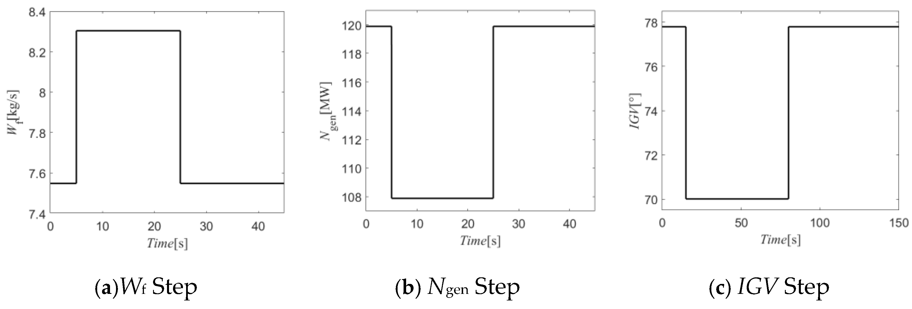
A 10% step disturbance is applied to the fuel flow rate, power generation power, and guide vane angle, respectively. By comparing the variation laws and dynamic response differences of two key measurable parameters n and T₇ under different sensitivity parameter values, the influence characteristics of each sensitivity parameter on the model dynamic response are evaluated, and the differences between the two modeling methods are compared. The step input variations in W_f, N_gen, and IGV are shown in Figure 10.

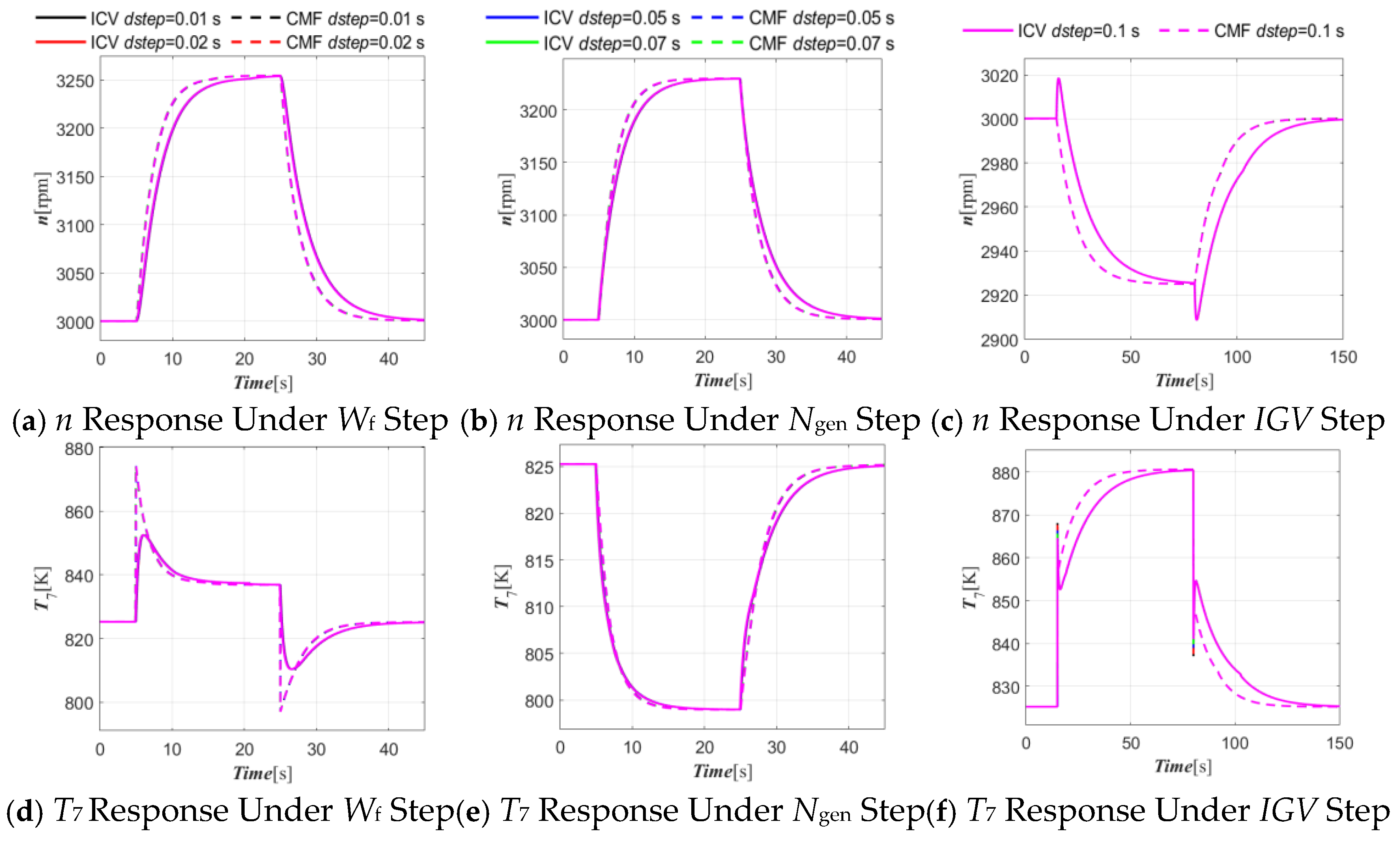
Set the sampling time interval dstep to 0.01 s, 0.02 s, 0.05 s, 0.07 s and 0.1 s. The responses under different dstep values are compared in Figure 11. It can be seen from the figure that whether the ICV method or the CMF method is adopted, within the step size range given in this paper, the transient responses of n and T₇ basically coincide, making the sub-figure in Figure 11 appear to have only two curves; that is, within a certain range of sampling step sizes, the numerical errors caused by discretization fall within an acceptable range, and the numerical integration also exhibits good stability and convergence. Therefore, dstep is more reflected as a parameter setting at the numerical solution level here. When dstep is small enough that the integration errors of the state equation no longer dominate the results, continuing to reduce dstep mainly brings an increase in calculation burden, but the improvement to the result is limited. However, even if the two dynamic models are not sensitive to dstep, there will still be differences between the two methods in the early stage of step disturbance. That is, CMF emphasizes flow balance and iterative matching at each step, so the dynamic response is often faster and closer to the immediate change, while ICV allows flow imbalance and mass accumulation in the dynamic process, so the response is relatively smoother and closer to the actual dynamic process. Moreover, when step disturbance is applied to W_f, the maximum change amplitude of T₇ in ICV is lower than that in CMF. In addition, in the ICV method, when step disturbance is applied to IGV, the change in IGV will directly cause a sudden change in the compressor flow rate, which is quickly transmitted to the downstream components. According to the volume dynamic equation, the sudden change in flow rate in the early stage of disturbance will also lead to sudden changes in various parameters, and even the amplitude of the sudden change is larger than that in the CMF method.

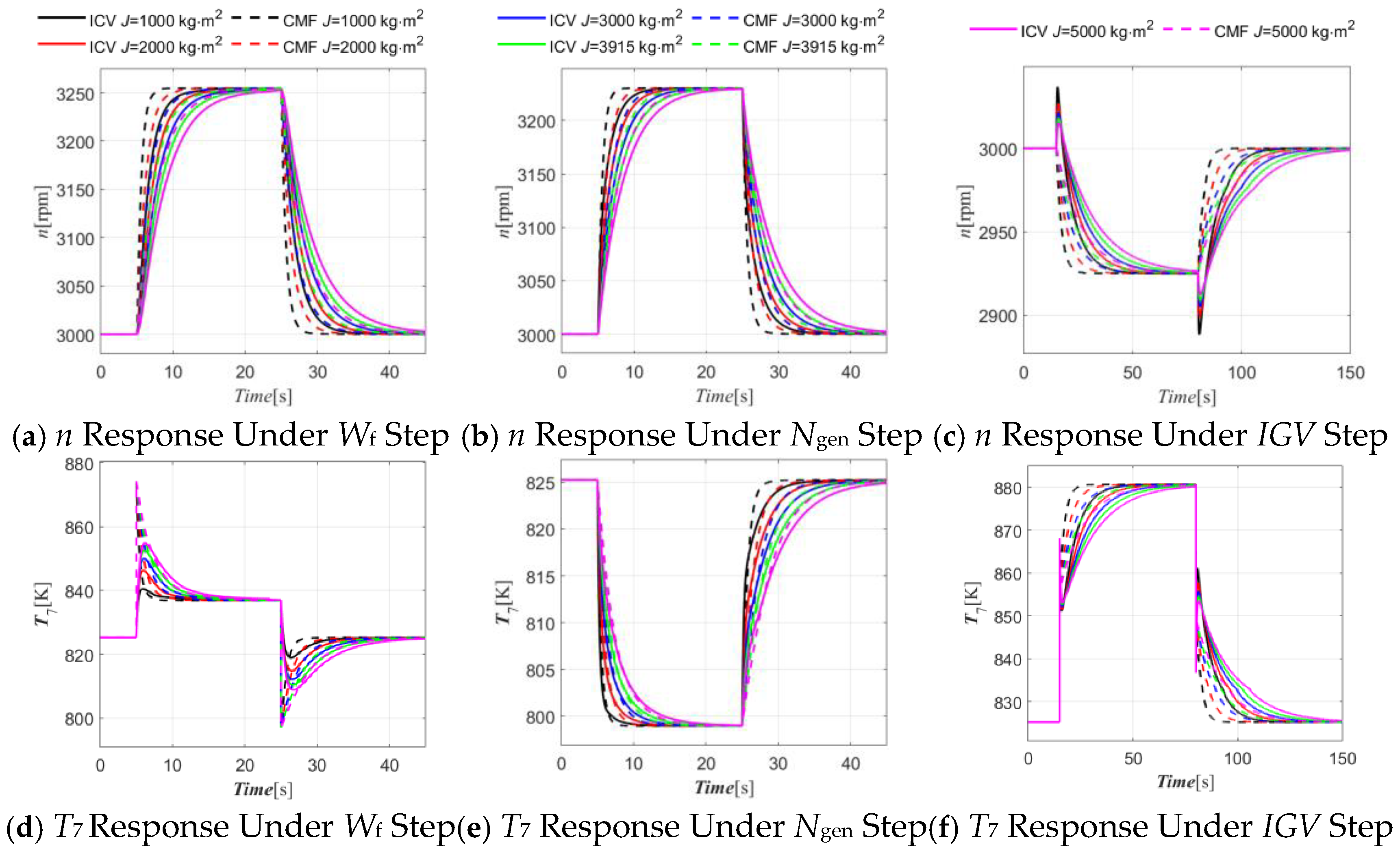
Set rotational inertia J to 1000 kg·m², 2000 kg·m², 3000 kg·m², 3915 kg·m², and 5000 kg·m². The response comparisons under different J are shown in Figure 12. It can be seen that when J is small, the slope of the rise or fall of n is larger, and the time required to reach a new steady state is shorter. As J increases, n change becomes slower and slower. This is because the rotor dynamics is driven by power imbalance, and J as an inertial term directly determines the speed of the dynamic response of n. J also indirectly affects the temperature response. Due to the different acceleration changes, the dynamic distribution in the combustion and turbine work processes will be different. Therefore, as J increases, the response time of T₇ will also slow down. Under different J values, there are obvious differences between the two methods. Under the same J, the n response of the CMF method is faster, and the transient peak of T₇ is more obvious. However, the ICV method allows the accumulation of mass and energy in the control volume, so the overall response is smoother. Moreover, when step disturbance is applied to W_f, as J increases, the peak amplitude of T₇ under the ICV method will also increase, accompanied by the delay of the peak occurrence time, which is consistent with the lag of the gas path thermodynamic process caused by the enhanced shafting inertia. However, regardless of the value of J, the peak of T₇ under the CMF method is almost the same.

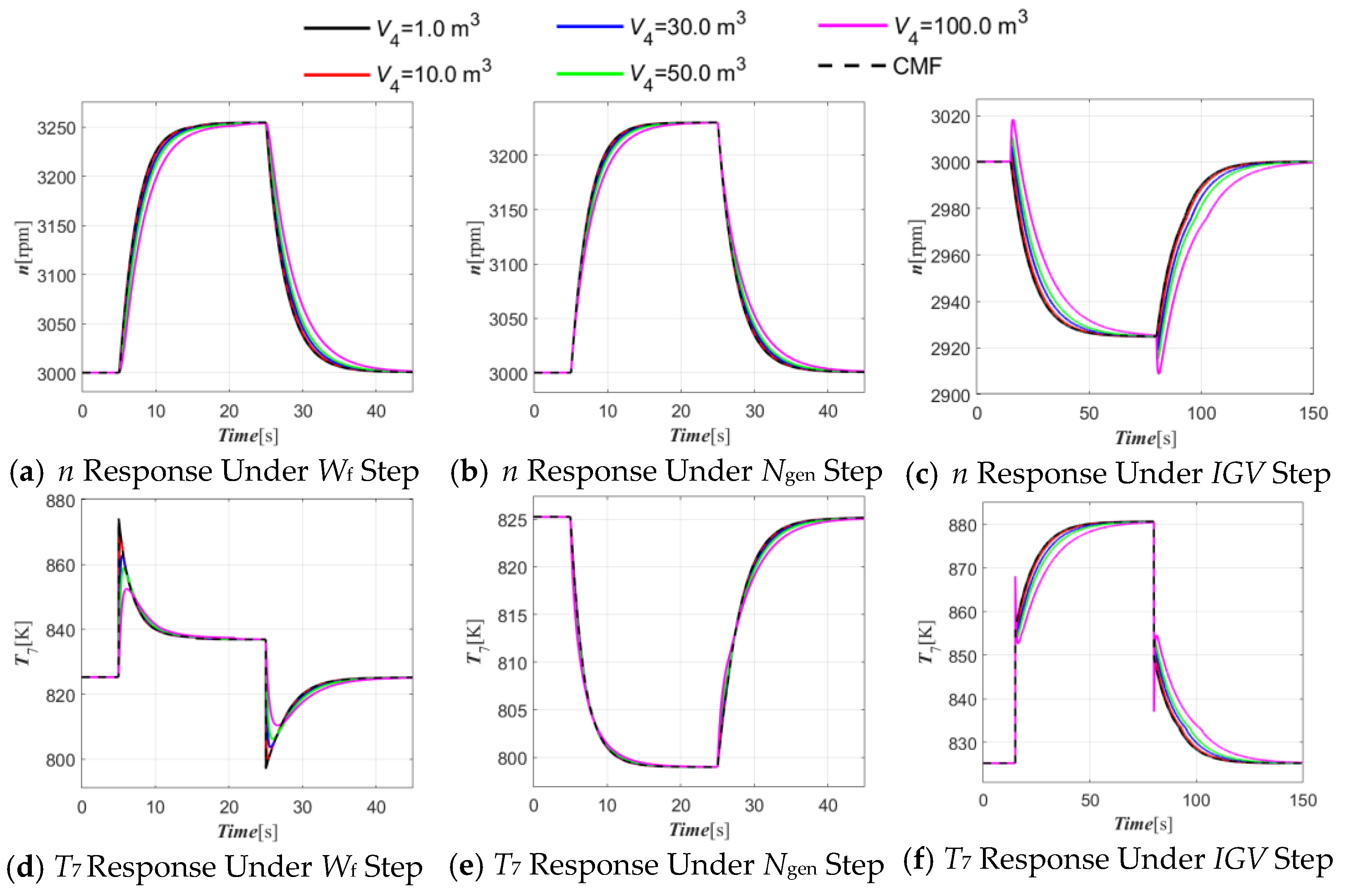
Set V₄ to 1 m³, 10 m³, 30 m³, 50 m³, and 100 m³. The responses under different V₄ values are shown in Figure 13. For the ICV method, the change in V₄ will significantly affect the dynamic change process of pressure and temperature, thereby changing the dynamic response of the system. It can be seen from the curves that as V₄ increases, the dynamic responses of n and T₇ tend to be smooth; that is, the rates of their rise or fall become slower. When step disturbance is applied to W_f, the peak of T₇ will also decrease accordingly; when V₄ decreases, the volume effect will be weakened, and the dynamic response model under the ICV method will be closer to the CMF method characteristic of no energy storage and instantaneous balance. However, even when V₄ is small, the dynamic response of ICV is generally smoother than that of CMF, indicating that the mass and energy accumulation effects introduced by the control volume state equation still exist within a certain range. It is worth noting that when step disturbance is applied to IGV, as V₄ increases, the transient fluctuation amplitude of n and T₇ in the early stage of disturbance is more significant. This is because the larger control volume makes the mismatch caused by the sudden flow change unable to accumulate and release within a longer time, thus showing more obvious short-term fluctuations on the curve.

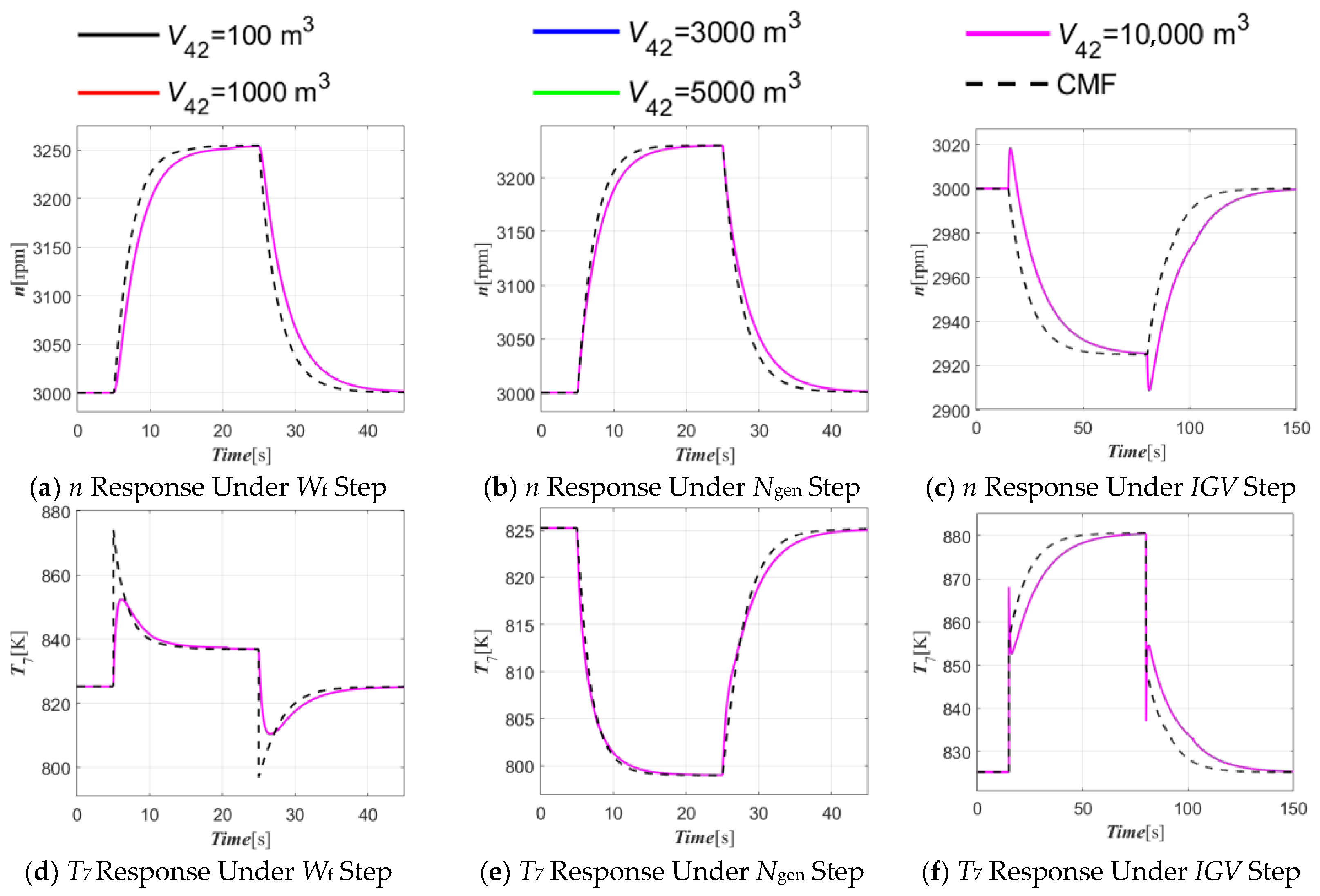
Set V₄₂ to 100 m³, 1000 m³, 3000 m³, 5000 m³, and 10,000 m³. The responses under different V₄₂ values are shown in Figure 14. Compared with V₄, the variation in V₄₂ exerts a relatively weak dynamic influence on n and T₇. Across a wide range of V₄₂ variations, the response curves under different V₄₂ values are almost coincident, indicating that the control volume here has a limited impact on the system dynamics. The reason is that V₄₂ is located after the gas turbine, and the pressure fluctuation of the downstream volume has a weak influence on the upstream parameters. Meanwhile, for the measurable parameters selected in this section, the dynamic response is mainly determined by the rotor inertia and combustor volume dynamics, while the diffuser section volume has a greater impact on the downstream pressure recovery process, thus showing low sensitivity. That is, not all volumes will equally dominate the dynamic process, and the intensity of sensitivity depends on the coupling strength between the volume and the main energy or mass accumulation links. However, for the two different dynamic modeling methods, although the influence of V₄₂ on the dynamic response is limited, the response of the ICV method under different V₄₂ values is generally smoother and the response process is slower than that of the CMF method. At the same time, under the W_f step, the peak value of T₇ in the ICV method is still smaller than that in the CMF method. In the actual modeling process, the real volume of the gas turbine outlet diffuser section will not be particularly large. However, to ensure the numerical calculation stability of the exhaust diffuser, the virtual volume V₄₂ is usually not set too small to avoid excessive transient fluctuations in the outlet pressure. In engineering, a method of applying gradient constraints to the mass conservation equation of the gas turbine outlet diffuser section is also commonly used to limit the pressure variation and improve the numerical stability of the simulation.

In summary, changes in dstep and V₄₂ have little impact on the dynamic simulation results. For dstep, a larger step size can be selected to reduce the computational load while ensuring convergence stability. Although V₄₂ is weakly sensitive to the responses of n and T₇, it is usually not set too small to ensure the numerical calculation stability of the exhaust diffuser. The rotor rotational inertia J is a highly sensitive parameter for both dynamic models, directly determining the dynamic response speed of n. In the absence of actual data during modeling, J should be calibrated first. Compared with J, V₄ is less sensitive, but a larger V₄ will still delay the dynamic response of each state variable. In terms of differences between dynamic modeling methods, the ICV method is more conducive to describing transient mechanisms and closer to the real physical state by introducing mass and energy accumulation in the control volume, but it may be sensitive to volume-related parameters. In contrast, the CMF method has fewer adjustable parameters and may exhibit more abrupt peak characteristics during large transient changes, requiring experimental data to verify rationality.

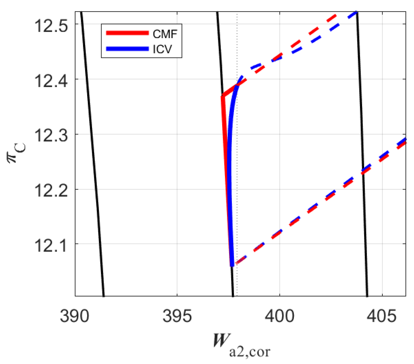
The two modeling methods not only differ significantly under fast transient operating conditions but also in the operating trajectories of component characteristics. Take the compressor characteristic line under W_f step disturbance as an example, as shown in Figure 15. In Figure 15, the black solid lines represent constant-speed lines, the red dashed and solid lines represent the operating trajectories under the CMF method, and the blue dashed and solid lines represent the operating trajectories under the ICV method. In terms of the operating trajectory of compressor component characteristics, the CMF method has obvious turning characteristics, while the ICV method is relatively smooth and continuous. This is because the CMF method enforces instantaneous matching at each step, making it easier for operating points to have obvious turning points in component characteristics. In contrast, the ICV method introduces inter-component control volumes, giving pressure and flow changes a certain dynamic inertia, thereby making the change process of operating points in the characteristic map more continuous and the trajectory smoother.

5.2. Comparison of Dynamic Operating Condition Results

A segment of actual operating data of the gas turbine is selected, and the corresponding inputs of P₀, T₀, W_f, N_gen, and IGV for this segment of operating data are shown in Figure 16. This segment of actual data is used as the input of the gas turbine model to compare the simulation accuracy and dynamic tracking capabilities of the two dynamic modeling methods under actual operating conditions. Combined with the sensitivity analysis results in Section 5.1, two sets of parameters are selected for analysis: the first set is dstep = 0.02 s, J = 3915 kg⋅m², V₄ = 2 m³, V₄₂ = 200 m³; the second set is dstep = 0.02 s, J = 3915 kg⋅m², V₄ = 100 m³, V₄₂ = 200 m³. That is, only V₄ differs between the two sets, and J adopts the reference value provided in the technical specification. The simulation errors of each set of parameters are shown in Figure 17. The simulation curves under the first set of parameters are shown in Figure 18 and those under the second set in Figure 19, where OD in the legends of both figures denotes operational data and SD denotes simulated data. The performance comparison under different parameters and different modeling methods is shown in

Table 11. Simulation performance comparison under different parameters.

	Modeling Method	V4 = 2 m3	V4 = 100 m3
Time Consumption	ICV	1.837 s	1.738 s
	CMF	5.011 s	4.846 s
Number of Component-Level Model Calls per Step	ICV	5	5
	CMF	8	8
MAE	ICV	0.184%	0.162%
	CMF	0.184%	0.184%

.

It can be seen from Figure 17, Figure 18 and Figure 19 that the simulation results under the two sets of parameter settings are very close, with most of the simulation results overlapping. However, when V₄ takes a larger value, the dynamic response lag of the model is more obvious compared with when V₄ takes a smaller value. It can be seen from Table 11 that regardless of the set of parameters, compared with the CMF method, the ICV method has shorter computation time consumption, fewer calls to the component-level model per step, and higher computational efficiency. When V₄ takes a smaller value, the errors of the two sets of parameters are consistent. After increasing V₄, the simulation accuracy of ICV simulation is improved, but the simulation accuracy of both is still very close. Since the input changes during actual operation are usually relatively continuous and there are no idealized abrupt operating conditions, the difference between the two models under this measured data segment is limited. Although the distinction between CMF and ICV in terms of accuracy is not high, the ICV method has obvious advantages in computational efficiency, making it more conducive to rapid simulation and application in engineering scenarios.

6. Conclusions

Taking the PG9171E single-shaft heavy-duty industrial gas turbine as the research object, this paper establishes steady-state and dynamic component-level mechanism models based on thermodynamic modeling ideas, and conducts model correction and dynamic comparison research. The main conclusions are as follows:

(1)

The adoption of three improvement strategies, namely Tent chaotic mapping initialization, improved convergence factor, and TAO, can effectively solve the problem of the original Dung Beetle Optimization algorithm falling into local optimal solutions, significantly improve the optimization accuracy, and achieve better convergence performance on most test functions.

(2)

Based on actual operating data, the improved DBO algorithm is used for gas turbine model correction, reducing the maximum model error from 3.1% to 1.01 × 10⁻⁵%, which significantly improves the accuracy of the gas turbine simulation model.

(3)

Sensitivity analysis and comparison are carried out on the two types of dynamic models (ICV and CMF). The results show that the rotor rotational inertia J is a highly sensitive parameter for both types of models, V₄ will delay the response of state variables to a certain extent, while dstep and V₄₂ have little impact on the results. Compared with the CMF method, the dynamic response of the ICV method has a certain lag and is closer to the actual physical process, and the operating trajectories of component characteristics are also different. In addition, the ICV method has shorter simulation time and is more suitable for rapid simulation and application in engineering scenarios.

(4)

The developed gas turbine model in this study is established and calibrated based on the PG9171E unit and its on-site operational data; therefore, the specific model parameters and quantitative results are primarily applicable to the PG9171E configuration. Nevertheless, the proposed mechanism-based modeling framework and the correction methodology are general and can be extended to other gas turbine types, provided that the corresponding component maps and correction factors are re-identified and re-calibrated using the target unit’s data.

(5)

Future work will focus on deploying the proposed model and correction workflow in an online digital-twin setting. By integrating real-time operational data, the correction factors can be updated periodically to account for ambient variations and progressive degradation, enabling online performance monitoring and health assessment.