Article

Sensitivity Analysis and Design of Dynamic Inductive Power Transfer Coil Geometries for Two-Wheeled Electric Vehicles Under Misalignments

by
Mário Loureiro
1,
R. M. Monteiro Pereira
1,2,3 and
Adelino J. C. Pereira
1,2,3,*
1
Coimbra Institute of Engineering, Polytechnic University of Coimbra, Rua Pedro Nunes–Quinta da Nora, 3030-199 Coimbra, Portugal
2
SUScita—Research Group on Sustainability, Cities and Urban Intelligence, Coimbra Institute of Engineering, Polytechnic University of Coimbra, Rua Pedro Nunes, 3030-199 Coimbra, Portugal
3
INESC Coimbra—Instituto de Engenharia de Sistemas e Computadores de Coimbra, Pólo II, 3030-290 Coimbra, Portugal
*
Author to whom correspondence should be addressed.
Energies 2026, 19(6), 1456; https://doi.org/10.3390/en19061456
Submission received: 9 February 2026 / Revised: 2 March 2026 / Accepted: 11 March 2026 / Published: 13 March 2026

Abstract

This work investigates the geometric design and optimisation of a dynamic inductive power transfer coupler for two-wheeled electric vehicles under misalignment and magnetic-field exposure constraints. A computational three-dimensional finite-element model of a shielded rectangular coupler is developed to characterise coupling coefficients and magnetic flux density levels on control planes along the longitudinal travel range and under lateral and angular misalignments. Two simulation datasets are generated: one varying only geometric parameters at a nominal position for surrogate construction and global sensitivity analysis, and a second jointly sampling geometry, the travel range and misalignments for optimisation. Sparse Polynomial Chaos Expansions and Canonical Low-Rank Approximation surrogates are built to quantify Sobol’ indices, revealing that a small subset of primary-side geometric variables dominates both coupling efficiency and magnetic field levels. Random forest regressors are then trained on the extended dataset and embedded in the Non-dominated Sorting Genetic Algorithm II to solve a multi-objective optimisation problem that maximises worst-case coupling, improves robustness to misalignment, and enforces magnetic-field leakage limits. Optimal designs were obtained, and a subset was selected for re-evaluation using the finite-element method. The results confirm that the proposed surrogate-assisted framework yields coupler geometries with enhanced coupling and reduced magnetic field leakage while respecting the mechanical constraints for the electric motorcycle system.

1. Introduction

Dynamic inductive power transfer (DIPT) systems have been proposed as an approach for the harmonious integration of electric mobility into electrical urban infrastructure. Nevertheless, there are technical challenges related not only to the intrinsic characteristics of the technology but also to the specific operational demands of each vehicle category. For electric vehicles (EVs) with two wheels, significant technical difficulties are associated with stabilising coupling stability under frequent misalignments. Alongside this challenge, particular attention must also be given to compliance with the applicable standards regulating magnetic field exposure.
In this work, these challenges are addressed at the coupler design level. The focus is placed on the development of a constrained design and analysis framework for DIPT coil systems dedicated to micromobility, combining finite element analysis, surrogate-based global sensitivity analysis, and multi-objective optimisation. The goal is to explore how coil geometries can be shaped to enhance power-transfer performance while respecting EMF exposure constraints on defined control planes along representative misalignment trajectories. In this context, Section 1.1 sets out the specific objectives and scope of the work.

1.1. Objectives

IPT systems are currently heading into a more advanced stage of development, with many studies being conducted on simulation and design using finite element analysis (FEA). However, the DIPT variant, which allows EVs to be powered, is still under development, and studies are needed on its efficiency, misalignment tolerance, and EMF leakage control.
The aim of this work is to design and validate a constrained optimisation pipeline for DIPT coil systems for two-wheeled EVs that maximises power transfer efficiency while ensuring EMF compliance on defined controlled planes across longitudinal motion under lateral or angular misalignment.
This contribution will focus on the following objectives:
  • Develop a physics-based electromagnetic model of a representative DIPT system on a FEA solver to characterise performance along a longitudinal motion of the secondary coil over the primary coils, including lateral and angular misalignments;
  • Construct a structured simulation dataset that relates relevant geometric variables, movement parameters, and misalignment scenarios of functional outputs, as well as spatial magnetic-field distributions on defined control planes;
  • Develop scalable surrogate or response-surface models to enable rapid exploration of the design space and to provide computationally efficient objective and constraint evaluations within an NSGA-II-based multi-objective optimisation framework;
  • Formulate and solve a multi-objective coil-geometry optimisation problem using NSGA-II, ensuring compliance with electromagnetic exposure limits on the control planes along the entire vehicle trajectory;
  • Assess the robustness of candidate designs to expected variations, evaluating efficiency and field compliance under perturbed conditions;
  • Provide practical recommendations for DIPT coil geometry and operating conditions that balance efficiency, compliance with EMF limits, and dimensional constraints, thereby providing actionable guidance for subsequent work.
Having defined the design objectives and the corresponding performance metrics, the next step is to enable their efficient evaluation across a large design space. High-fidelity simulations provide the required accuracy, but their computational cost can become prohibitive when embedded in iterative optimisation and robustness studies. For this reason, the following section introduces surrogate modelling techniques to approximate the relevant response functions and presents sensitivity analysis to quantify how each design variable influences the selected outputs. This methodological step supports rapid exploration of trade-offs and provides clear guidance on which parameters most strongly drive performance before proceeding to optimisation.

1.2. Workflow Overview

The overall workflow of the computational framework adopted in this work is represented in Figure 1, clarifying how the high-fidelity finite-element model is coupled with the surrogate-assisted optimisation stages. The process begins with a design of experiments (DoE) strategy used to sample the relevant design space and to generate simulation data from the finite-element model. Two complementary datasets are then constructed from these simulations in order to quantify the influence of the geometric design variables under a nominal configuration and enable computationally efficient multi-objective optimisation over the combined geometry-misalignment domain.
The first dataset (1) is generated under the nominal alignment condition by varying only the geometric design variables. It is employed to construct sparse PCE and canonical LRA surrogate models, from which Sobol indices are computed to rank the relative importance of the geometric variables and to support the interpretation of the resulting design trade-offs (Figure 1). In parallel, the second dataset (2) is generated by varying both the geometric variables and control variables, namely lateral and angular misalignment and longitudinal movement. This dataset is used to train a random forest surrogate, which acts as a fast evaluator within the NSGA-II genetic algorithm for multi-objective optimisation under misalignment-factor constraints. After obtaining the Pareto front, a reduced set of candidate designs is selected, and one final design is chosen. This design is subsequently re-evaluated using the finite-element model to verify the surrogate-based predictions.

2. Surrogate Techniques and Sensitivity Analysis

The design of complex electromagnetic systems requires significant computational resources, which increase the costs incurred during the design phase. As stochastic modelling considering uncertainty in physical phenomena is increasingly being applied to engineering projects, it requires dealing with large amounts of information that demands significant computational resources. Monte Carlo simulation is one of the most commonly used methods, allowing statistical quantities to be estimated by repeatedly sampling inputs and re-evaluating the model a large number of times. For studies requiring high fidelity, the number of re-evaluations can easily reach thousands or millions of runs, resulting in extremely high computational costs [1].
Surrogate modelling is an alternative that aims to generate a mathematical model that functionally approximates a high-fidelity computational model. As each evaluation of a finite element solver is costly, a carefully validated model can reduce orders of magnitude of computational resources while retaining the input–output structure needed for prediction, optimisation, and sensitivity analysis. However, surrogates for design engineering should be substantially cheaper than the parent model and sufficiently accurate for decision-making purposes [2].
The model is created based on the response of the computational model to specific inputs and is trained to approximately predict the response of the computational system, reducing calculation time and computational costs. Surrogate models facilitate rapid and practical analysis, allowing the acquisition of a series of detailed analyses as well as sensitivity analysis and uncertainty quantification.

2.1. Surrogate Techniques and Notation

In the previous section, a qualitative overview of surrogates was introduced. In the present section, the discussion is formalised by introducing the mathematical notation that will be applied through this work.
Consider a random input vector with independent components X = ( X 1 , . . . , X M ) R M , endowed with a joint probability density function (PDF) f X ( x ) . In this work, unless otherwise stated, the components X i are assumed to be mutually independent (Equation (1)).
f X ( x ) = i = 1 M f X i ( x i )
A surrogate model is a computationally inexpensive approximation of the high-fidelity model M , trained from a design of experiments,
D = { x ( i ) } i = 1 N R M , y = ( y ( 1 ) , . . . , y ( N ) )
where y ( i ) = M x ( i ) . The high-fidelity model response is defined as the random variable Y = M ( X ) . Based on the training data ( D , y ) , a surrogate mapping M * is constructed such that Y * = M * ( X ) M ( X ) [3,4].
The following subsections introduce the surrogate families considered in this work, as well as random forest regression and the theoretical foundations of sensitive analysis.

2.2. Canonical Low-Rank Approximations

Canonical low-rank approximations (LRAs) constitute a class of surrogates that use tensor-product structures in order to mitigate the curse of dimensionality. The main objective is to approximate the response of a deterministic computational model by a sum of a small number of rank functions. Each rank function is written as a product of univariate functions in the individual input variables. In contrast to PCE, which works on an expanded multivariate polynomial basis, canonical LRA is separated from the tensor product, leading to a number of unknown coefficients that increase linearly with the input dimension of the original model for fixed polynomial degrees and rank. This property makes LRA particularly attractive for high-dimensional problems where the number of instances is relatively limited [5,6].

2.2.1. Mathematical Formulation

As in previous sections, a deterministic computational model M mapping an input random vector X = ( X 1 , . . . , X M ) with a joint PDF f x onto a scalar response Y with independent components X i and associated marginals f X i is used (Equation (3)).
X D X R M Y = ( M ) R
A rank-one function of X is defined in Equation (4), where each v ( i ) is a univariate function on the i-th input variable.
w ( X ) = i = 1 M v ( i ) ( X i )
A canonical low-rank approximation of rank R N is then obtained by expressing the model response as a finite sum of the rank-one components in Equation (5), where a r R are scalar weighting factors and v r ( i ) denotes the univariate function in the i-th dimension associated with the r-th rank-one term.
M L R A ( X ) = r = 1 R a r i = 1 M v r ( i ) ( X i )
For minor values of R, this representation yields a canonical low-rank approximation of the deterministic computer model [6].

2.2.2. Advantages

Canonical LRA reduces the number of unknown coefficients relative to a full multivariate polynomial chaos expansion of similar degree by exploiting a sum of rank one tensor products. When the response admits a low canonical rank, the number of coefficients and least squares problems scale approximately linearly with input dimension [5].
The method is non-intrusive and can be built from input–output pairs using alternating least squares with regularisation and cross-validation for rank selection [6,7]. Orthonormal polynomial bases enable analytic computation of moments and Sobol indices through coefficient post processing, supporting efficient global sensitivity analysis [5,7,8].

2.2.3. Limitations

Performance depends on the existence of a low-rank representation. If the response contains strong high-order interactions across many inputs, the required rank may increase substantially, eroding benefits over polynomial chaos expansion and potentially leading to slow convergence or local minima in alternating least squares iterations [7].
Implementation is comparatively intricate. Beyond selecting polynomial degrees and truncation, one must define alternating least squares update rules, stopping criteria, and rank selection strategies, which increases methodological sensitivity. In many practical studies, polynomial chaos expansion is therefore adopted as the default surrogate, with low-rank approximation used selectively [9].

2.2.4. Applicability to the Present Study

The deterministic model is a three-dimensional finite element representation of a dynamic inductive power transfer coupler with a moderately high-dimensional input space. It includes transmitter and receiver geometry and misalignment variables, while simulation budgets remain constrained. This setting favours canonical low-rank approximation due to its coefficient scaling with input dimension.
Analytic expressions for mean, variance, and Sobol indices support variance-based global sensitivity analysis under geometric and positional uncertainty. Polynomial chaos expansion is retained as the primary surrogate because of established practice and simple closed-form Sobol indices [9]. Low-rank approximation will be used in parallel to cross validate sensitivity rankings.

2.3. Polynomial Chaos Expansions

Polynomial chaos expansion (PCE) occupies a distinctive position as an uncertainty quantification method [10]. The primary objective of PCE is to construct a surrogate of the original deterministic computer model. In PCE, the model response is represented as a series expansion in terms of the ability to represent the model response with a high level of accuracy. The following subsection presents the basic principles of PCE, its mathematical formulation, and its application to the current study.

2.3.1. Mathematical Formulation

In the PCE framework, the model response is expressed as an expansion in terms of orthonormal polynomials of the input random variables. Let X = X 1 , . . . , X M R M be a random vector with independent components, characterised by a joint PDE f X ( x ) in a domain D X R M . Consider a deterministic computational model Y = M ( X ) , Y R with finite variance (Equation (6)) so that Y belongs to the space of square-integrable random variables.
D X M 2 ( x ) , f X ( x ) , d x < ,
Under these assumptions, PCE provides a spectral representation of M ( X ) on the basis of multivariate polynomials that are orthonormal to f X [4].
The model response can be written as in Equation (7), where α = α 1 , . . . , α M N M is a multi-index that identifies the polynomial degree in each input variable, Ψ α ( X ) is a multivariate polynomial that is orthonormal with respect to f X , and c α R are the corresponding expansion coefficients.
Y = M ( X ) = α N M c α Ψ α ( X )

2.3.2. Advantages

PCE represents the model response in an orthonormal polynomial basis consistent with the input distributions. Statistical moments follow directly from the coefficients. Orthonormality yields an exact variance decomposition, so the first order and total Sobol indices are obtained analytically through coefficient post processing, without further model evaluations [4].
Sparse PCE is non-intrusive and requires only deterministic finite element runs on an experimental design. Hyperbolic truncation and least angle regression promote compact expansions by selecting a small active polynomial set that captures dominant effects and low-order interactions, enabling efficient surrogate-based Sobol analysis [4,11].

2.3.3. Limitations

The candidate basis grows combinatorially with input dimension and polynomial degree, creating a challenging selection problem [4,12]. Even with sparsity promotion, accuracy depends on whether a limited set of terms can represent the relevant interactions within the available training budget.
PCE is most effective for smooth responses. Localised features or sharp gradients may require high degrees, reducing stability and increasing cost. The surrogate is also conditional on the assumed input distributions and dependence structure, which affect the orthonormal basis and coefficient interpretation [12].

2.3.4. Applicability to the Present Study

The characteristics of the present DIPT case study are aligned with the assumptions under which regression-based sparse PCE is effective. The number of uncertain inputs, consisting of the geometric design variables and the misalignment parameters, remains moderate, and the Maxwell-based model yields responses for the coupling coefficients and magnetic flux density that vary smoothly over the corresponding design domain. Under these conditions, a sparse polynomial basis can represent the dominant trends and low-order interactions with relatively few active terms, so that accurate estimates of moments, Sobol indices, and tail probabilities can be obtained at very limited additional cost once the coefficients have been identified [4,11].
In conclusion, PCE is suitable for the subsequent analysis carried out in the present work. A single DoE of Maxwell simulations is used to construct separate surrogates for the key outputs, and these surrogates are then employed for global sensitivity analysis and as inexpensive models in the multi-objective optimisation study.

2.4. Random Forest Regression

Random forest regression is a method that combines a large number of decision trees into a single predictive model. Each tree is built by repeatedly splitting the input space into smaller regions using rules that aim to group together training observations with similar response values. To enable diversity among the trees, each one is grown on a resample of the original training data, and, at each split, only a random subset of the input variables is considered. For a new input, every tree assigns the point to one of its terminal regions and predicts the mean of the training responses within that region. The random forest prediction is obtained by averaging the outputs of all trees, which tends to reduce prediction variance while preserving the ability to represent complex, non-linear relationships between inputs and outputs. This construction can be interpreted as a particular form of bootstrap aggregation in which many over-fitted but low-bias trees are combined to produce a more stable regression function [13,14].
The random selection of input variables in each split further decorrelates the trees, which improves the effectiveness of the averaging step. Random forests can be viewed as local-averaged data-adaptive estimators that approximate the regression function by aggregating information from training observations that fall in similar regions of the input space. This perspective explains why random forests are particularly effective in problems where interactions between inputs play an important role [13,14].

2.4.1. Advantages

Random forest regression offers several properties that make it attractive for engineering applications. It does not require the specification of an explicit functional form for the input–output relationship: the partitioning induced by the trees adapts automatically to the structure of the data and can represent strong non-linearities and interactions without prior assumptions about their form. The use of many trees, each fitted to a perturbed version of the data, together with the averaging of their predictions, leads to a substantial reduction in variance compared to a single decision tree and typically provides good predictive accuracy with limited tuning settings [13].

2.4.2. Limitations

Random forest predictors are piecewise constant and therefore not smooth, which limits their suitability for derivative-based analysis and for optimisation methods that require smooth response surfaces. They also lack controlled extrapolation, so predictions outside the training domain or in sparsely sampled regions may be unreliable averages of distant observations [14].
Interpretability is limited because the regression function has no compact analytic form, unlike spectral surrogates. Moments and variance-based sensitivity measures are not available in closed form and typically require Monte Carlo sampling on the surrogate, adding numerical error. Performance also depends on hyperparameter tuning to avoid under or over fitting [13,14].

2.4.3. Applicability to the Present Study

In the present study, random forest regression is used as a surrogate model to support the NSGA-II algorithm in the multi-objective optimisation of geometric design parameters. A forest is trained on a dataset of DoE Maxwell simulations, using as inputs the geometric variables and misalignment parameters, and as outputs the quantities that define the optimisation objectives and constraints, such as the coupling coefficients and the maximum magnitude of the magnetic flux density. Once trained, the forest provides fast and reasonably accurate predictions over the design domain spanned by the training data, which makes it suitable for repeated evaluations within an evolutionary optimisation loop.
For the NSGA-II algorithm, the random forest serves as a surrogate that allows the evaluation of candidate geometries. This significantly reduces the computational cost of exploring large populations and many generations while preserving the main trends and interaction effects captured in the original simulations. The optimisation search is explicitly restricted to the region of the input space covered by the training designs, and a selected optimal candidate design from Pareto fronts is subsequently re-evaluated with the Maxwell model to verify the surrogate predictions. In this way, the random forest acts as an efficient screening tool that enables practical multi-objective optimisation of the DIPT coupler geometry under geometrical restrictions.
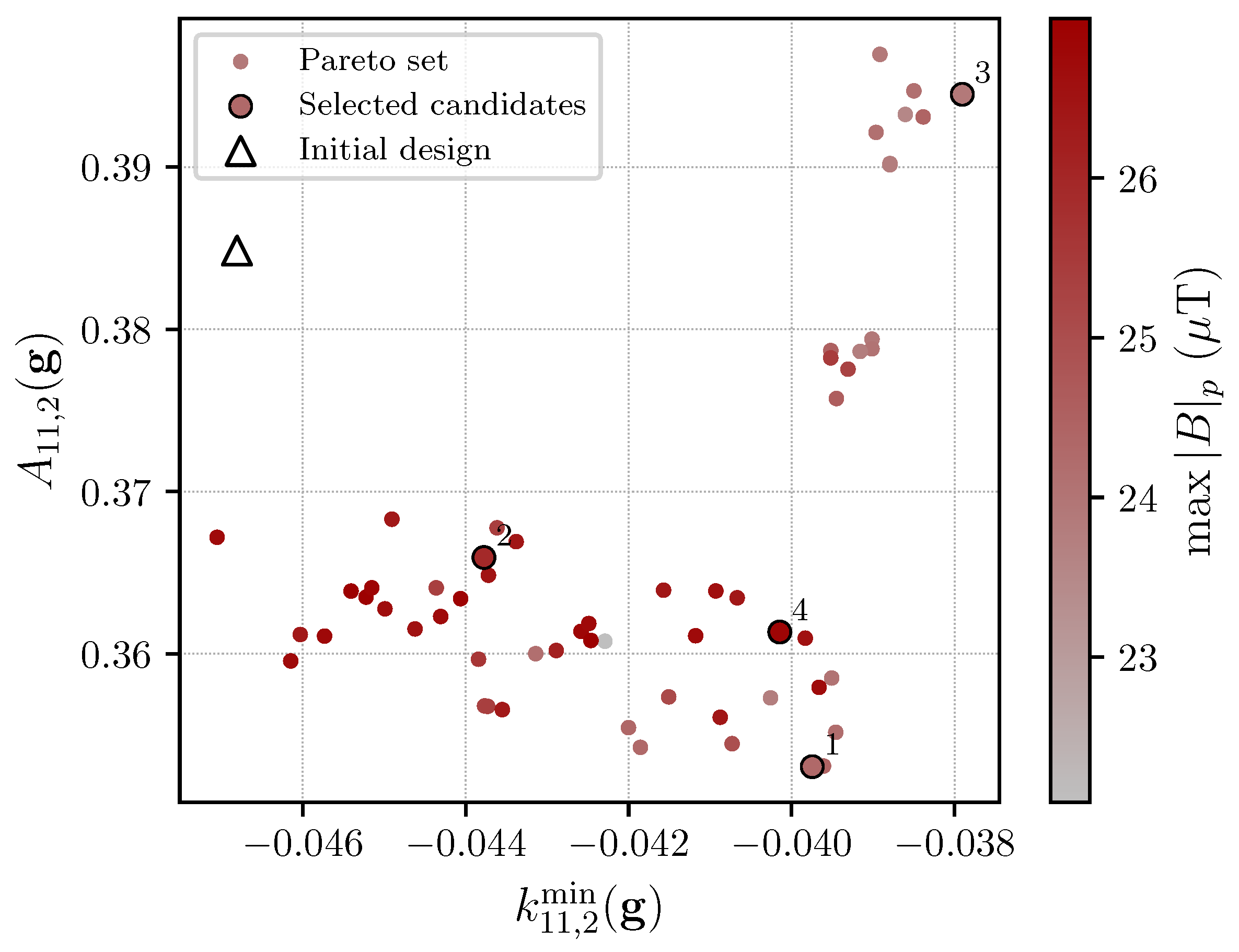
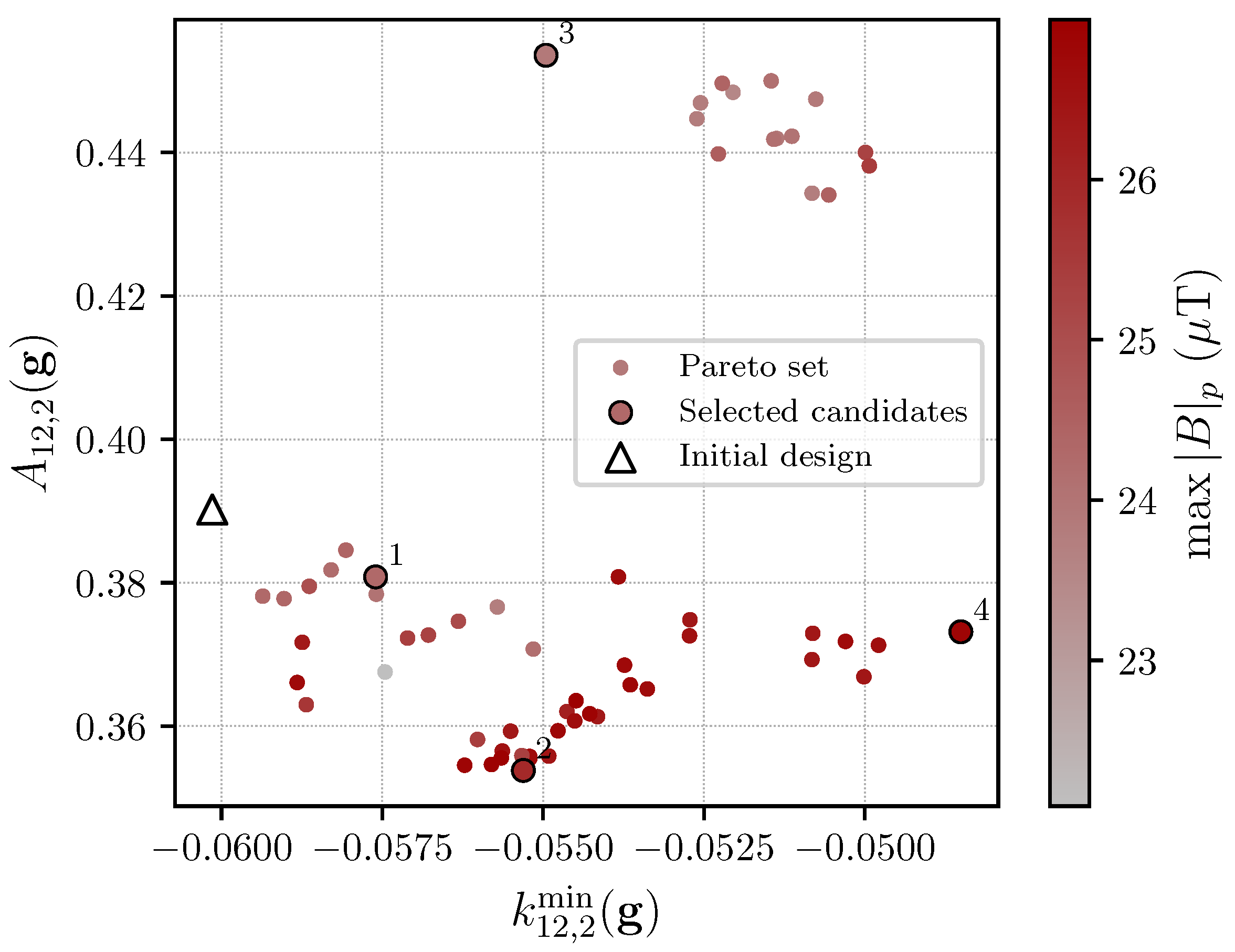
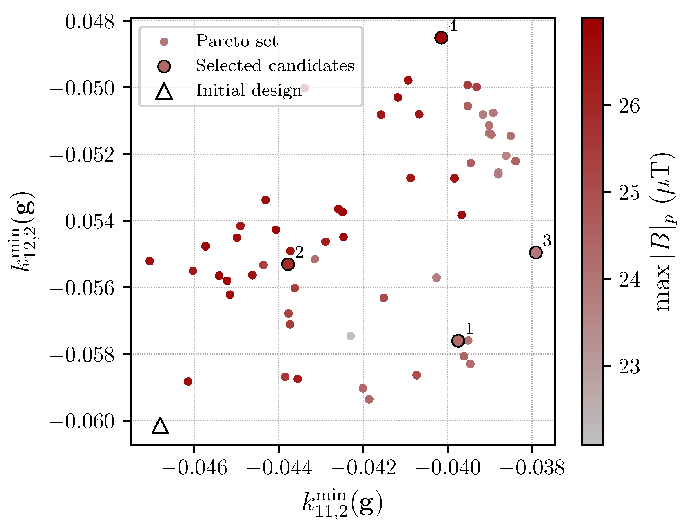
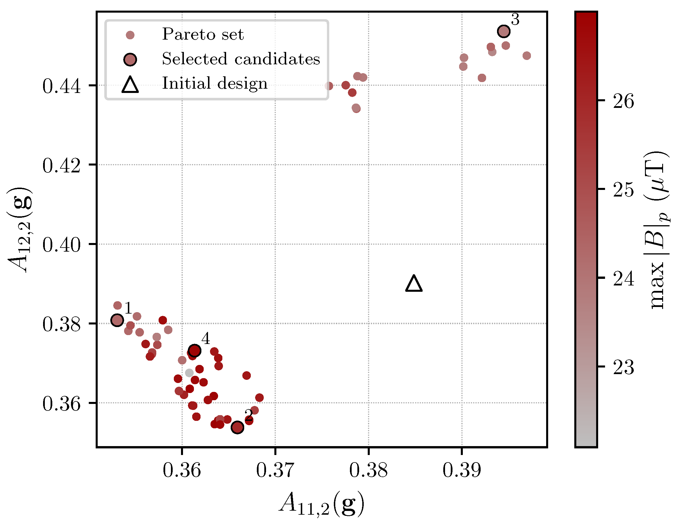
In practical terms, the integration is realised by using the random forest as an evaluator within the NSGA-II optimisation process. After training the model on the DoE, NSGA-II generates candidate geometries that are assessed via the surrogate rather than by new finite-element runs. The predicted responses are then used to compute the solution to the multi-objective constraints. After analysing the resulting Pareto fronts, candidate design 3 is selected as the preferred compromise with respect to the targeted performance criteria and is subsequently re-evaluated using the finite-element model to confirm the surrogate-assisted optimisation outcome.

2.5. Global Sensitivity Analysis

Global sensitivity analysis (GSA) enables quantification of the correlation between certain input parameters and output parameters in a deterministic computational model. The process begins by decomposing the variance of the model output as a function of the contributions of each individual input parameter [15].
Approaches to GSA can be classified into sample-based methods, linearisation methods, and global methods. Sample-based methods analyse correlations based on Monte Carlo samples. Linearisation methods are applicable to linear models or models that can be linearised around a given value. They are not applicable to non-linear models or those with high-order interactions. The Perturbation method and the Cotter method are referred to. Global methods are capable of evaluating linear and non-linear models by observing their variance and distribution. Morris’ elementary effects, Borgonovo sensitivity indices, and Sobol indices are cited, which will be applied in this study [9].

2.6. Sobol Indices

The variance of a deterministic computational model can be determined by the sum of the variances of the inputs to that model. Variance-based global sensitivity analysis aims at quantifying how the uncertainty in each input variable, and in their possible interactions, contributes to the overall variance of a model’s output [9].
The first-order and total Sobol indices associated with each input variable are the most relevant quantities used in engineering applications. The first-order Sobol index of X i is defined by Equation (8).
S i = D i D = Var E ( Y X i ) Var [ Y ] .
The total Sobol index of X i , denoted S T i , aggregates the main effect of X i and all interaction effects in which X i participates. It is defined as the sum of all Sobol indices that involve X i ,
S i T = { i 1 , , i s } i S i 1 , , i s ,
which is not convenient for computation because it would require evaluating every higher-order index. Instead, an approximation can be made by computing the sensitivity measure for all variables except the one that is being evaluated S i T = 1 S i .

3. Finite Element Analysis

The study and optimisation of resonant DIPT systems is still a technical challenge, opting for methods that use FEA simulation or the analytical deduction of mathematical expressions that define the electromagnetic behaviour of the coupling. Computer simulations require the prior execution of a three-dimensional model, the configuration of materials, and other physical aspects. They require a considerable amount of simulation time and consume a vast amount of computing resources due to the analysis of many complex variables and mesh optimisation. Research efforts have focused on the surrogate modelling of resonant IPT systems [16,17]. However, investigations specifically addressing the dynamic aspects of these systems remain absent from the current body of literature. Currently, research on the design of resonant DIPT systems specifically geared towards micromobility applications remains absent. This manuscript aims to address this research gap by contributing to the field of resonant DIPT systems focused on micromobility. The initial phase involved the construction of a detailed three-dimensional representation of the system specifically tailored for an e-motorcycle, followed by electromagnetic simulation [18].
Ansys Maxwell 2025 R2 software was employed to perform electromagnetic simulations, given its reputation as a reference tool in the industry and applicability to the system in question. Presented as a tridimensional and bidimensional eddy current solver for electromagnetics, the software allows field parameters to be calculated as well as representation of the magnetic fields created. The solver employs adaptive meshing techniques that require the definition of the geometry, material properties, electric excitation, and required output data. Adaptive meshing is applied throughout the iterative solving process, reducing error and eliminating the need to define a mesh with complex geometry. The Ansys Maxwell magnetic transient solver enables the transient study of moving models, circuit coupling, and induced eddy currents based on the application of volumetric meshing and is applicable to resonant DIPT systems. Section 3.1 discusses the initial geometry of the model under study and its dimensions.

3.1. Model Geometry

The model under study is dimensionally similar to References [16,19]. In Study [19], the coupling efficiency in the transition between primary coils was optimised using a supplementary coil. However, the results indicated that this supplementary coil generated peaks when passing over the transition section. Consequently, the initial setup in this study consisted of two primary coil assemblies that were rectangular in shape. Each coil had its length extended significantly to reach 2000 mm, as this is a more economical option and reduces the number of passages by transition per distance travelled.
The secondary coil was adapted to the size of the rear wheel of an e-motorcycle. A rectangular coil surrounding the rear wheel was chosen for compactness and to allow manoeuvrability without interfering with objects passing by the sides of the vehicle or accidental contact with the ground. Its design is based on the idea presented in Reference [20]. The design of the shield has been extended to promote the reduction of the magnetic field density in the upper area where the driver of the vehicle is located. Figure 2 illustrates the topology of the model to be optimised.
The geometry of the model was built directly in the Ansys Maxwell environment using parametrised dimensions associated with optimisation variables. The model was implemented using named parameters for all relevant lengths and widths, allowing automatic manipulation and optimisation by parametric calculation. Table 1 summarises the variables to be optimised, their symbology, and their initial values. The selected parameters include the interior and exterior width and length dimensions of the coils, shielding, and ferrite layers, the distance between these elements, as well as the number of primary and secondary coil windings.
The parameters mentioned in Table 1 and illustrated in Figure 2 were selected as the most influential in terms of coupling, power transfer efficiency, and the robustness of the system to misalignments. Figure 3 represents the geometrical parameters over a top view and a side view of the coupling. The parameters were implemented as named variables in Maxwell, allowing a study of systematic variation in a parametric study that supports the construction of a dataset. This dataset will be a tool for capturing the impact of each variable in the face of different misalignment scenarios along the movement of the vehicle and its secondary coil along the primary coils on the roadway.
The geometry of the primary coil defines the distribution of the magnetic field along the respective segment of the road, which critically influences the efficiency under conditions of alignment and misalignment. Increasing the size of the primary coil improves tolerance to lateral misalignment, since the secondary coil remains within the main flux region for a greater distance. However, increasing the size of the primary coil reduces the flux density in the area where optimal alignment is achieved, contributing to a reduction in mutual inductance. It also increases the volume of copper required, which translates into an increase in coil resistance and losses. Therefore, the dimensions of the primary coil must balance the efficiency of the coupling, energy losses, and tolerance to misalignment.
The geometry of the secondary coil, which is mounted on the vehicle, is constrained by space and weight limits. The dimensions of the inner and outer width of the secondary coil and the outer length were selected so that the geometry could be optimised according to the compromise between integration compactness and sufficient area to intercept the magnetic flux generated by the primary coil. A smaller secondary coil increases power density but is less tolerant of misalignment, while a wider coil is more robust to misalignment but increases weight, cost and reduces efficiency in perfect alignment.
Ferrite plates are used to provide a low-reluctance path for magnetic flux, guiding it through the coupling region and reducing leakage to the neighbourhood. The flux controller improves the mutual inductance between the primary and secondary coils, improving the efficiency of the transferred power and reducing EMF leakage to meet ICNIRP standards. The length of the ferrite influences the primary and secondary coils in significantly different ways. The ferrite layer in the primary coil helps to confine the magnetic field in the roadway, ensuring that the flux generated interacts with the secondary coil instead of dispersing into the ground and surroundings. Although ferrite improves performance on misalignment, its extension well beyond the area of the coil increases the cost and complexity of the installation without a significant gain in efficiency. For road infrastructure, the increase in weight is not as relevant as it is for the secondary system, but the mechanical robustness of the driveway and the cost of materials and installation are. In the case of the secondary coil, the ferrite serves to guide the flux through the coil area, maximising the induced current and tolerance to lateral and angular misalignment. However, increasing the surface area of the ferrite increases the weight on the vehicle. Ferrite is brittle, so its application in vehicles requires special care in the design phase in favour of its durability. For both the primary and secondary systems, varying the size of the ferrite has little effect on the energy transfer efficiency. The SAE J2954 standard states that the ferrite should extend slightly beyond the perimeter of the coil and that the increase in benefit from the improvement in energy transfer efficiency cancels out with the increase. The aim of this study will also be to identify the optimum range of ferrite extension for each of the systems.
Conductive shielding is necessary to limit stray magnetic fields and contribute to the regulation of exposure regulations. The application of shielding on the roadway underneath the primary system is provided for in the SAE J2954 standard, helping to reduce EMF losses and exposure to pedestrians [21]. A shield with considerable dimensions helps to contain the magnetic field. However, increased shielding increases eddy current losses, which generate heat and degrade the system’s efficiency. This effect is especially relevant at 85 kHz, where induced currents cause thermal issues. The total weight is not critical for the primary installation, but thermal dissipation and energy loss impose an upper limit.
Secondary shielding is designed to protect vehicle occupants and sensitive electronics from EMF leakage. It also prevents induced currents in the vehicle’s metal parts. Increasing the secondary shield increases the weight of the vehicle and the size of its base, which is the upper limit. There will be a point at which increasing the shielding area will not improve EMF leakage over region 3 referred to by SAE J2954 [21]. Shielding must be dimensioned to meet the limits established in the applicable standards while maintaining eddy current losses within acceptable limits.
The position along the longitudinal movement in the direction of EV circulation is given by the variable x, where this value comprises the total length of the two primary coils.
Misalignments are classified as lateral misalignments, where the position of the vehicle is offset from the axis of symmetry of the primary system, and angular misalignments, where the vehicle is inclined in relation to the plane orthogonal to the plane of the primary coils (Figure 4).
Table 2 presents the movement and misalignment control variables. The vertical separation (air gap) between primary and secondary assemblies is fixed in this study at z = 150 mm.

3.2. Model Construction

For brevity, the detailed finite-element model construction is provided in the Supplementary Materials (Section S1). This includes the definition of the global and relative coordinate systems used to apply secondary-side displacement and misalignment (Figure S1), as well as the definition of the magnetic-field leakage control planes and the justification for the chosen plane locations according with the applicable standards (Figure S2).

3.3. Materials and Electromagnetic Properties

In this section, the materials selected for simulation in Ansys Maxwell are presented. The selection of materials and their electromagnetic properties is essential for modelling the real behaviour and efficiency of the system. The properties were selected according to the IEC 61980-3 [22] and SAE J2954 standards [21,23].

3.3.1. Windings

Litz wire was used to model the coil windings, having an external diameter of 5 mm placed adjacently, in accordance with the guidelines of the SAE J2954 standard [21]. The use of this type of conductor is based on its capability to mitigate eddy current losses. The properties of the copper incorporated in the windings are presented in Table 3.
The SAE J2954 standard refers only to the outer diameter of the litz wire, without mentioning other construction aspects. For a specific operation frequency, it is possible to determine the number and diameter of strands and sub-bundles needed to mitigate the effects of the skin effect and proximity effect. The skin effect is the tendency of current in an AC circuit to flow along the outer edges of the conductor, resulting in increased electrical resistance. The proximity effect is the tendency of current to flow in undesirable patterns, such as loops or concentrated distributions, due to the presence of magnetic fields generated by nearby conductors.
The skin depth δ can be determined by Equation (10), where ρ represents the resistivity of the copper conductor, f represents the frequency of the sinusoidal current in the winding, and μ 0 represents the permeability of free space.
δ = ρ π f μ 0
The litz wire is constructed in copper and is subjected to a test temperature of 20 °C, with a resistivity of ρ = 1.72 × 10 8   Ω · m. The operating frequency f is 85 kHz and the permeability of free space is 4 π × 10 7 H/m. The skin depth for the case study is approximately 0.2264 mm. The diameter of a single wire should be, at most, approximately one-third of the skin depth [24]. The maximum theoretical diameter for a single wire considering this orientation should be 0.075 mm. Consulting a catalogue from a manufacturer, for example, Elektrisola, it emerges that the calculated value is close to the range of 0.079–0.102 mm for operating frequencies of 50–100 kHz, respectively, considering that the closest value by excess of commercial single wire diameters is 0.080 mm [24].
The litz wire must have an external diameter of 5 mm in accordance with SAE J2954 and a single wire diameter d s w of 0.080 mm. A taped cable with a 0.2 mm outer coating t O C of polyethylene naphthalate (PEN) was selected for thermal class 130–180 in accordance with standard EN IEC 60317-11 [25]. The packing factor k P F considered will be 1.30 [24].
O D L W = k P F · n s w · d s w + t O C
The number of single wires n s w for the case study will be 2130.18. This is rounded to 2000, as the number of single wires can vary by up to ± 25 % [26].
The length of the twist or length of lay shall not exceed 60 mm and shall have an ‘S’ twist (counter-clockwise), in accordance with standard EN IEC 60317-11 [25]. The length of lay is 20 mm, in accordance with the specifications of the manufacturer Elektrisola [27]. The twisted length factor (TLF) is considered in FEA simulation, referring to the ratio of the twisted-strand length to the bundle length. TLF is given by Equation (12), where n s w represents the total number of single wires in the litz wire, d s w the diameter of a single wire, k P F the packing factor and p the length of lay.
T L F = π 2 n s w d s w 2 4 k P F p 2
For the case study, given that the number of single wires is n s w = 2000 , d s w = 0.080 mm, the packing factor k P F = 1.3 and the length of lay or pitch p = 20 mm, the TLF will be approximately 1.061.

3.3.2. Ferrite

The ferrite cores integrated into the model are designed in strict accordance with the specifications defined in the SAE J2954 standard, which refers the use of TDK PC95 ferrite tiles. This directive is followed due to the 61980 standard guidelines, as these standards do not offer comprehensive guidance or detailed specifications regarding this particular matter. The SAE J2954 standard defines, for WPT1 systems (power classification up to 3.7 kVA) and ground clearances Z1 (100 to 150 mm) or Z2 (140 to 210 mm), the use of PC95 (TDK) ferrite, as well as the tests performed [21]. Table 4 represents the relevant properties for simulating the system in Ansys Maxwell.
The IEC 61980-1 and SAE J2954 standards state that practical tests should be conducted at a temperature of 20 ± 5 °C [21,29]. For this study, the B-H curve for 20 °C is obtained from the manufacturer’s curves for other temperatures. The curve is obtained using the anhysteretic components of the Jiles–Atherton model. The project parameters are M s = 4.435 × 10 5 A/m, a = 1.628 × 10 1 A/m and α = 2.689 × 10 5 [30]. Substituting this triplet into the implicit anhysteretic law produces a single-valued, solver-ready B ( H ) dataset.

3.3.3. Shielding

To confine EMF leakage and induced currents in nearby structural parts, a conductive plate of aluminium was modelled as a shielding. This approach follows established mitigation practices in IPT systems operating in the 85 kHz band defined for automotive wireless charging and is consistent with the compliance objectives set by SAE J2954 and IEC 61980-3 standards. SAE J2954 further provides practical guidance for vehicle and ground assemblies, including a minimum aluminium shielding plate thickness of 0.7 mm, which was adopted here as the baseline for FEA modelling. The IEC 61980-3 standard does not mention a thickness, but in the auxiliary drawings, it represents the shielding as 1 mm, without issuing guidelines regarding this measurement.
According to Reference [31], the field magnitude decays exponentially with depth. At an operating frequency of f = 85 kHz, using aluminium with μ r = 1.000 and σ = 38 × 10 7 S/m, the skin depth will be given by Equation (13).
δ = 2 ω μ σ = 2 2 π f μ 0 μ r σ = 0.28 mm
Considering the minimum thickness of 0.7 mm referred to in the SAE J2954 standard, it can be seen that it approximately follows the triple thickness rule to reduce the skin depth. Considering that the thickness t = 0.7 mm, and therefore t / δ = 2.5 , the decay of the magnetic field for a thickness t is given by Equation (14).
B ( t ) = B ( 0 ) e t / δ
Therefore, for a plate thickness t, the transmitted fraction would be approximately e t / δ . For the case study, it would be e t / δ = 0.008211 , meaning that only 8.2 % of the field amplitude would be transmitted, or 20 log 10 e t / δ = 2.7 dB.
Table 5 represent the electromagnetic properties assigned to the aluminium shielding in Ansys Maxwell.
Aluminium is modelled as non-magnetic, a good conductor, and as a shielding actuator reducing the magnetic field on the areas that do not contribute to the efficiency of the system.
The leakage-field constraint follows the ICNIRP low-frequency exposure guidelines, which report general-public reference levels as unperturbed RMS values. In the 3 MHz to 10 MHz band (covering 85 kHz), ICNIRP specifies a magnetic flux density reference level of 27 μT for the general public [33]. SAE J2954 adopts this same 27 μT limit for the standardised exposure-assessment regions accessible to occupants and the public (regions 2 and 3). IEEE C95.1 reports less strict reference levels for unrestricted environments in the same frequency range (for example, 205 μT for head and torso exposure) [34]. In this work, the leakage-control planes were placed to represent the SAE J2954 accessible regions (passenger-compartment and lateral and external vicinity) and to follow the standard test-point placement rationale. This enables future experimental measurements at the same locations and a direct comparison against the Maxwell results for additional conservatism and to maintain margin relative to the 27 μT reference level planes (Figure S2 in the Supplementary Materials).

3.4. Excitations and External Circuit

In this study, the primary coils are excited by a current-source regulated at 38 A (rms) at a frequency of 85 kHz. The transmitting side employs an SS compensation network. On the secondary side, the secondary coil also has an SS compensation network and powers a purely resistive 10 Ω load, which represents the equivalent input resistance of the rectifier and DC–DC stage of the on-board charger.
The use of an SS topology that powers a nominal resistive load is consistent with many IPT and DIPT prototypes reported for the charging of EVs, where transmission efficiency and transfer power are evaluated using series–series compensation under fixed load conditions [16,35].
Furthermore, selecting an operating frequency of 85 kHz aligns the design with the frequency band recommended by the SAE J2954 and IEC 61980-3, which specifies 85 kHz as the nominal resonant frequency for automotive WPT systems [21,22].
At this stage, the electrical interface is intentionally specified with fixed characteristics, thereby allowing the analysis to isolate the electromagnetic implications of coupler geometry and misalignment. In particular, the SS compensation is employed to enforce a consistent fundamental-frequency operating condition across the design space, and the receiver is represented by an equivalent resistive load. Within this modelling framework, the computed coupling coefficients and the maximum magnetic flux density on the control planes are intended to reflect the influence of the magnetic structure and relative positioning. Loss mechanisms in the compensation network and power electronic stages, including the equivalent series resistance (ESR) of the compensation capacitors, as well as tuning strategies, are not explicitly represented. Accordingly, the results should be interpreted as geometry-driven trends in coupling behaviour and magnetic-field exposure under misalignment rather than as a complete prediction of end-to-end efficiency.

3.5. Design of Experiments and Generation of Datasets

Two numerical datasets were constructed to support the surrogate modelling, sensitivity analysis and optimisation tasks, both having as outputs the coupling coefficients and the maximum magnitude of the magnetic flux density on the top, left and right control planes. The first dataset comprises 2200 instances and was generated by varying only the geometric design parameters of the coupler while keeping the relative position between the pads fixed at x = 1000 mm, y = 0 mm and α = 0. This dataset was specifically devised for the global sensitivity analysis: a sparse PCE surrogate model was identified from these samples, and the corresponding Sobol indices were computed to quantify the relative influence of each geometric variable. A second dataset, containing 2500 instances, was then constructed by sampling the control variables within the bounds 0 mm x 4000 mm , 300 mm y 300 mm and 20 ° α 20 °. This second dataset provides a joint representation of geometric and positional variability over the relevant misalignment space and forms the basis for the subsequent surrogate modelling and multi-objective optimisation studies. The geometrical boundaries are represented in Table 6.

3.6. Computational Infrastructure and Software

All numerical simulations and post-processing were performed on a dedicated HP Z620 workstation. The system is equipped with an Intel® Xeon® CPU E5–2620 0 running at 2.00 GHz, providing six physical cores and twelve logical processors, and with 128 GB of system memory. A discrete NVIDIA Quadro 410 graphics processing unit was used to support the graphical interface of the finite element pre- and post-processing tools. Analyses were performed using the Ansys Maxwell and Ansys Circuit modules within the Ansys Electronics Desktop Student 2025 R2 software.
This software suite was used to set up the three-dimensional finite element models, to solve the AC magnetic field problems for the different misalignment scenarios, and to extract the circuit-level quantities required for the subsequent optimisation and sensitivity analysis stages. The overall computational cost of this study was dominated by the repeated solution of these three-dimensional Maxwell models for different combinations of geometric parameters and misalignment conditions.

4. Global Sensitivity Analysis

This section presents the global sensitivity analysis of the DIPT system based on PCE surrogates. It begins by describing the construction, validation, and error metrics of the replacement models, as well as the definition of the training sets and the input and output variables. Next, the probability density functions of the responses are obtained, and the Sobol indices associated with the coupling coefficients and magnetic flux density in the control planes are calculated and discussed. Finally, the information provided by the sensitivity indices is synthesised to identify the most influential geometric parameters, analyse the trade-offs between coupling efficiency and exposure to electromagnetic fields, and support the selection of decision variables for the optimisation problem.

4.1. Construction and Validation of PCE Surrogate Models

The PCE surrogates were constructed in the UQ[py]Lab 1.0.0. framework from the electromagnetic simulation campaign performed in Maxwell. The input space is defined by the 22 geometric variables of the coupler, limited by the intervals in Table 6, from which 2200 geometric combinations were generated and evaluated.

4.1.1. Training Datasets and Input–Output Definition

The DoE in was generated in Maxwell using the Optimal Space-Filling (OSF) Design, which is an optimised Latin hypercube sampling maximizing the distances between experiments or points. This strategy ensures that no two points are too close to each other and that the variable bounding is fully populated and represented. In this setting, the OSF algorithm starts from a Latin hypercube sampling and iteratively repositions the points to maximise the minimum pairwise distance while preserving the constraints, which leads to an almost uniform coverage of the 22-dimensional input domain and is particularly suited to computer experiments and surrogate modelling. A pseudo-random seed equal to zero was used to make the resulting DoE reproducible [36].
The number of samples was selected as a compromise between accuracy and computational cost: for regression-based PCE, the size of the experimental design is typically chosen to be of the same order or a few times larger than the number of retained polynomial basis terms in order to obtain a well-conditioned least-squares system. A total of 2200 OSF points were therefore adopted as the maximum affordable sample size on the available hardware. The same DoE was used for all quantities of interest (coupling coefficients and maximum magnetic flux density on the control planes), and its suitability for surrogate construction was assessed a posteriori based on the cross-validation and error metrics discussed in Section 4.1.3.
The coupling coefficients are computed from the Maxwell-exported inductance matrix. For each primary segment p { 1 , 2 } , the coupling between the primary coil 1 p and the secondary coil 2 is defined in Equation (15), where M 1 p , 2 is the mutual inductance and L 1 p and L 2 are the self-inductances.
k 1 p , 2 = M 1 p , 2 L 1 p L 2 ,
The raw results were exported from Maxwell in several tables for coupling coefficients, magnetic flux density on the control planes, and other auxiliary outputs and subsequently consolidated into a single dataset. During this pre-processing stage, non-essential columns were removed, units were made consistent with the notation adopted in this work, and column names were harmonised.

4.1.2. Polynomial Basis, Truncation Scheme and Sparsity Strategy

Given that all geometric variables are modelled as independent uniform random inputs within the bounds of Table 6, the PCE surrogates are built in UQ[py]Lab using the tensor products of univariate orthonormal polynomials associated with the uniform distribution, which corresponds to a Legendre-type polynomial basis [37].
The training configuration summarised in Table 7 shows that all surrogates are built on the same experimental design, with 22 input variables and 2200 full model evaluations, while the degree of polynomial and the truncation parameters are tailored to each quantity of interest. The values represent the final evaluation on the PCE surrogates.
For the coupling coefficients k 11 , 2 and k 12 , 2 , the full basis contains 1875 candidate terms, so the least-squares system used to identify the PCE coefficients is determined. For the magnetic-flux-density surrogates, the hyperbolic truncation leads to smaller full bases, 826 to 848 terms, which increases this ratio to approximately 2.6, yielding more comfortable conditions for regression. After sparse regression, only 174, 87, 60, and 92 terms are retained for k 11 , 2 , k 12 , 2 , max | B | top , max | B | left and max | B | right , respectively. This reduction indicates that the information contained in the 2200 training samples can be represented by a relatively small subset of polynomial interactions, suggesting that the effective dimensionality of the problem is lower than the nominal 22 inputs and that the calibrated PCE surrogates are both parsimonious and adequately supported by the available training data.
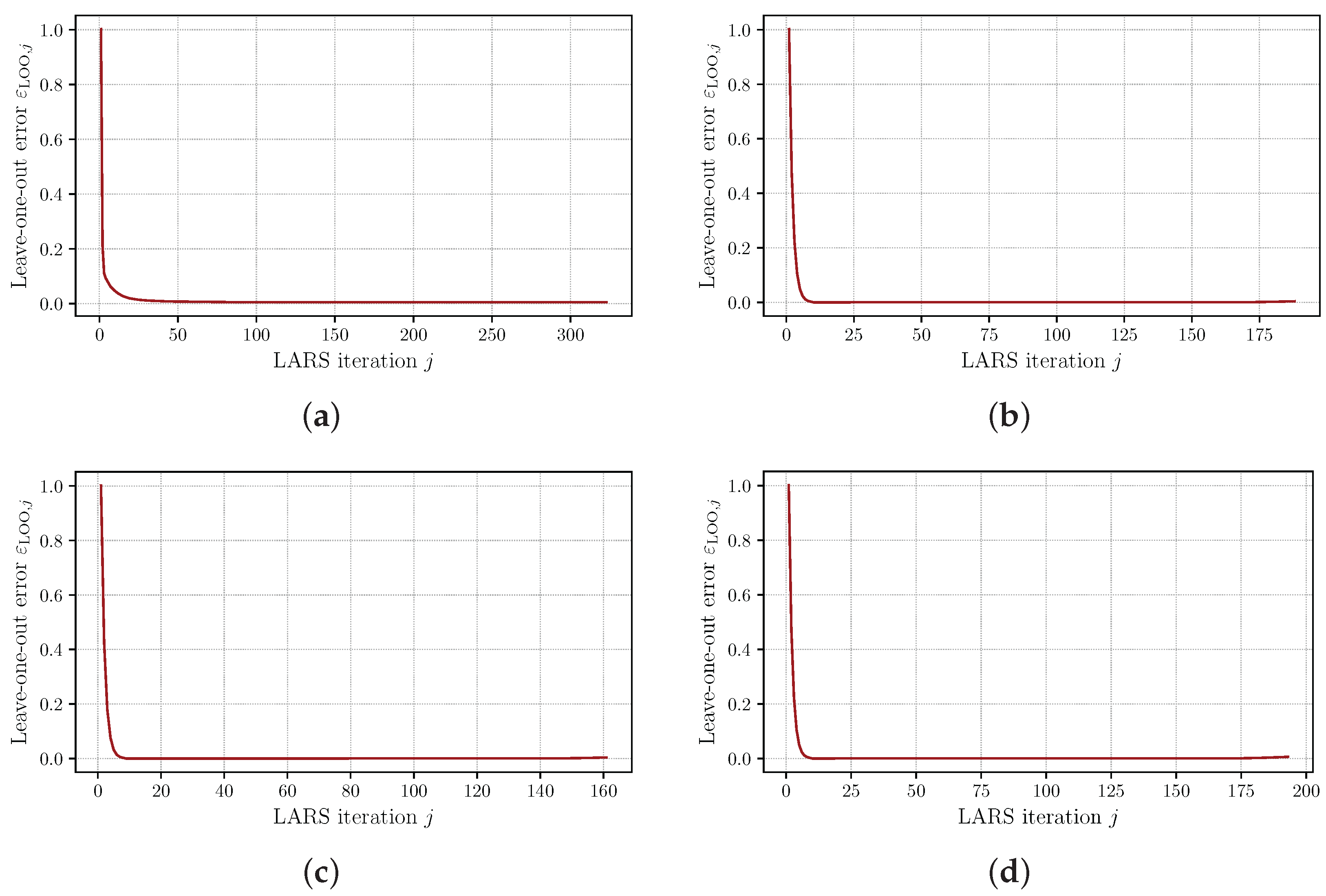
The convergence plots in Figure 5 represent, for all quantities of interest, the LOO error ϵ L O O decreasing very rapidly during the first LARS iterations and then approaching a plateau, indicating that only a relatively small number of basis functions is needed to capture the dominant response features. Figure 5a corresponds to the coupling-coefficient surrogates k 11 , 2   k 12 , 2 . It is visible that the error drops by several orders of magnitude within the first 20 to 30 iterations, after which additional terms provide only marginal improvements, which is consistent with the very small final ϵ L O O values in Table 8.
The magnetic-flux-density surrogates in Figure 5b–d represent a similar qualitative behaviour, with a steep initial decay followed by a slower convergence phase, although the asymptotic ϵ l O O levels remain higher than for the coupling coefficients, reflecting the stronger non-linearity of the responses. In general, Figure 5 confirms that the sparse PCE strategy produces stable surrogates whose predictive precision improves quickly with the number of active basis functions and then saturates, according to the basis sizes reported in Table 7.

4.1.3. Error Metrics

The validation metrics in Table 8 indicate that the PCE surrogates reproduce the original model responses with considerable accuracy for all quantities of interest.
The LOO error for the coupling coefficients k 11 , 2 and k 12 , 2 is ϵ LOO = 3.728 × 10 3 . For the magnetic flux density on the three control planes, the LOO errors are more pronounced but still relatively small. The modified LOO errors are only slightly larger than the original LOO errors for all outputs.
The remaining statistics provide further insight into how these errors compare with the natural variability of each response across the design space. The standard deviations of the PCE predictions are at least one order of magnitude larger than the corresponding LOO errors, showing that the surrogate models capture most of the underlying variation rather than numerical noise. The coefficients of variation, ranging from 18.390% for the coupling coefficients to about 27.674% for max | B | r i g h t , confirm that the responses exhibit substantial relative variability with respect to their mean levels, particularly for the lateral control planes. Because the surrogate errors are very small compared with both the mean and the standard deviation, the PCE models can be regarded as sufficiently accurate for global sensitivity analysis, where reliable estimates of trends and relative changes in k 11 , 2 , k 12 , 2 and the magnetic flux density are more important than reproducing individual simulations exactly.

4.2. Probability Density Functions

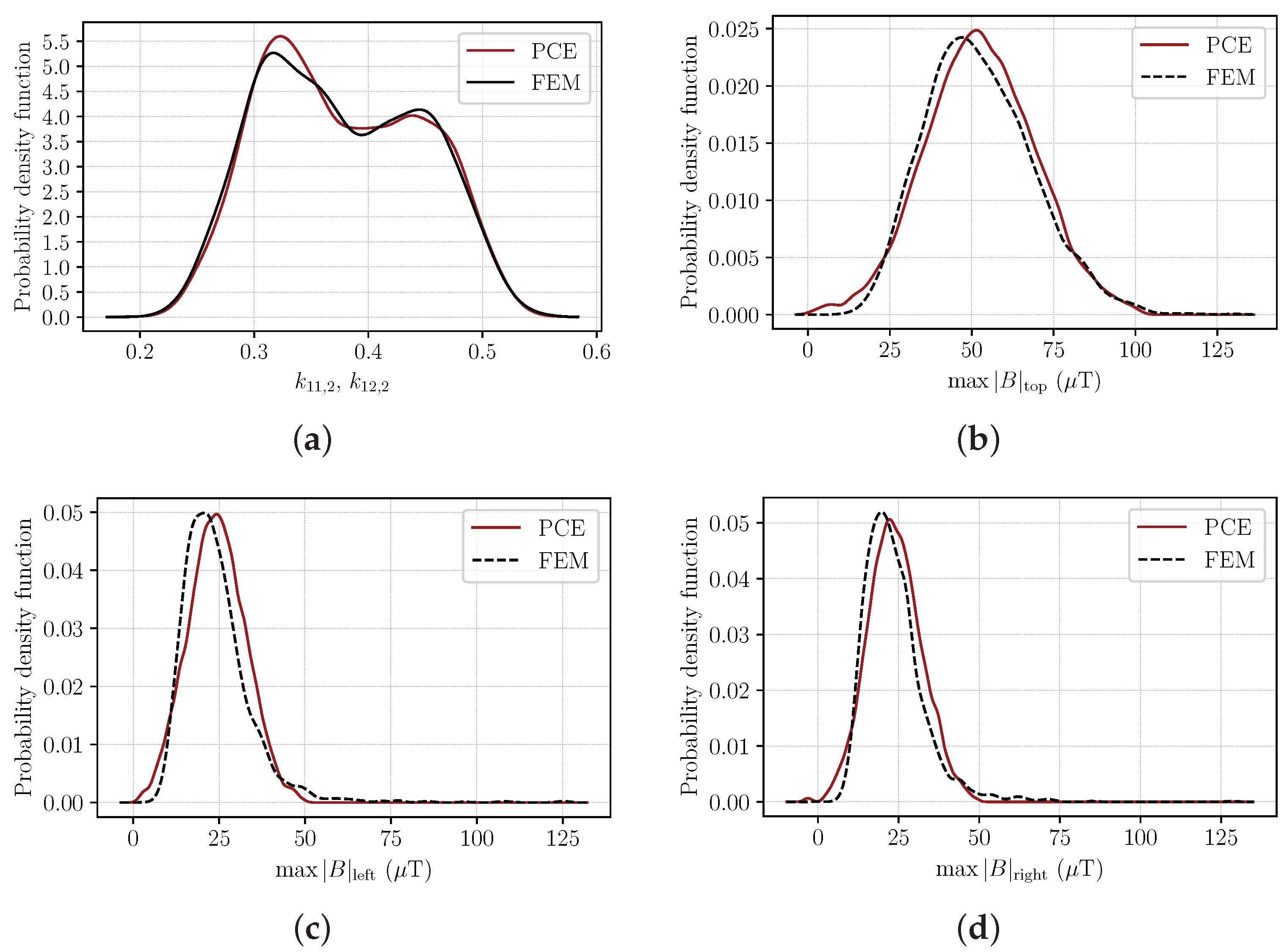
The agreement between the surrogate and the deterministic computational model can also be assessed by comparing the PDFs of the quantities of interest. Figure 6a represents the estimated PDF of the coupling coefficients k 11 , 2 and k 12 , 2 obtained from the PCE surrogate and from the FEM simulations.
The two curves almost coincide over the whole support of the distribution and exhibit the same multimodal structure, with a dominant mode around k 0.33 and a secondary shoulder at higher coupling values. The PCE curve is slightly smoother and presents a marginally higher peak probability, which is consistent with the small but LOO errors reported in Table 8. Overall, the surrogate accurately reproduces both the location and the shape of the distribution of the coupling coefficients, including the tails.
A similar level of agreement is observed for the maximum magnitude of the complex magnetic flux density on the three control planes, as depicted in Figure 6b–d. For the top plane, the PCE and FEM PDFs are almost indistinguishable, with the generic shape centred around max | B | top 55 μ T and a comparable spread.
For the lateral planes, the PCE PDFs retain the same qualitative shape as the FEM curves and peak at very similar values of max | B | left and max | B | right , although a slight systematic shift towards higher flux densities and a marginal broadening of the distributions can be observed. These differences are small in magnitude when compared with the overall width of the distributions and with the variability reported in Table 8, confirming that the PCE surrogates capture not only the mean response but also the uncertainty structure of the magnetic field with sufficient accuracy for the subsequent sensitivity and optimisation studies.

4.3. Sensibility Analysis

4.3.1. Sensitivity of the Coupling Coefficients

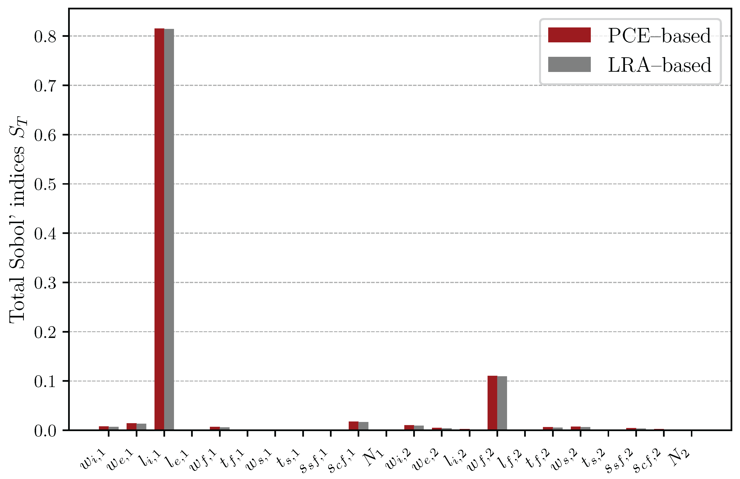
The total Sobol indices S T obtained for the coupling coefficients k 11 , 2 and k 12 , 2 are represented in Figure 7, showing a highly concentrated sensitivity pattern. When the geometric parameters are ordered by decreasing S T , the interior length of the primary coils l i , 1 clearly dominates the variance decomposition, with S T 0.815 . The second most important parameter is the exterior width of the secondary ferrite w f , 2 with S T 0.110 . Together, these two geometrical variables account for approximately 92.5 % of the output variance. The next group of parameters has markedly smaller, but non-negligible, contributions: the space between the primary coils and the ferrite s c f , 1 ( S T 0.018 ), the exterior width of the primary coils ( w e , q ) ( S T 0.014 ) and the interior width of the secondary coil w i , 2 ( S T 0.011 ). All remaining geometric parameters have total indices below 2 × 10 2 , the most relevant among them being the spacing between the primary coils and the widths of the ferrite and secondary coil, whose values are in the range of 10 2 to 10 3 . The parameters associated with the thickness of the shield, as well as the number of windings, have negligible total indices ( 10 4 ). This pattern indicates that the variance of k 11 , 2 is mainly controlled by the longitudinal extent of the primary coils l i , 1 and, to a lesser extent, by the transverse ferrite footprint on the secondary side w f , 2 , while most other dimensions act as second-order influences. When organised by subsystems, the primary coils represent the majority of the influence ( S T 0.840 ), followed by the ferrite of the secondary coil ( S T 0.125 ) and the primary ferrite ( S T 0.026 ). The shields account for only about 0.01 0.02 .
The prominent role of the interior length of the primary coil l i , 1 in the present sensitivity pattern is repeatedly shown to depend strongly on the length and width of the coil. For rectangular couplers, the study in [38] agrees with the finding that variations in the longitudinal dimension dominate the response of the coupling. Similar trends are reported in the broader DIPT literature, where coil length and segment geometry are identified as dominant drivers of coupling behaviour in dynamic configurations [39,40].
The width of secondary ferrite w f , 2 emerges as the second most influential parameter and also plays a role that is compatible with previous studies of ferrite plate optimisation in DIPT. The authors of Reference [41] studied a parametric optimisation of a 3 kW DIPT prototype and showed that the coupling factor is highly sensitive to the effective ferrite area and only weakly sensitive to its thickness in the non-saturated regime. In the present model, the relatively large S T ( w f , 2 ) together with the much smaller total effects of the thickness of both ferrites ( t f , 1 , t f . 2 ) are consistent with this research.
The week influence of shield dimensions and spacing between coils and ferrite mainly represents a fine tuning of the leakage-field distribution and local field homogeneity rather than affecting the overall coupling. This statement agrees with studies in which ferrite shielding and spacings are adjusted to balance field-confinement and loss, while the dominant trends in coupling are still imposed by the coil dimensions themselves. In the present sensitivity results, this is reflected by the fact that ferrite dimensions on the receiver side still show non-negligible S T , while shield-related parameters, which primarily shape leakage rather than main flux, have near-zero total effects on the coupling coefficient once the principal coil dimensions are fixed.
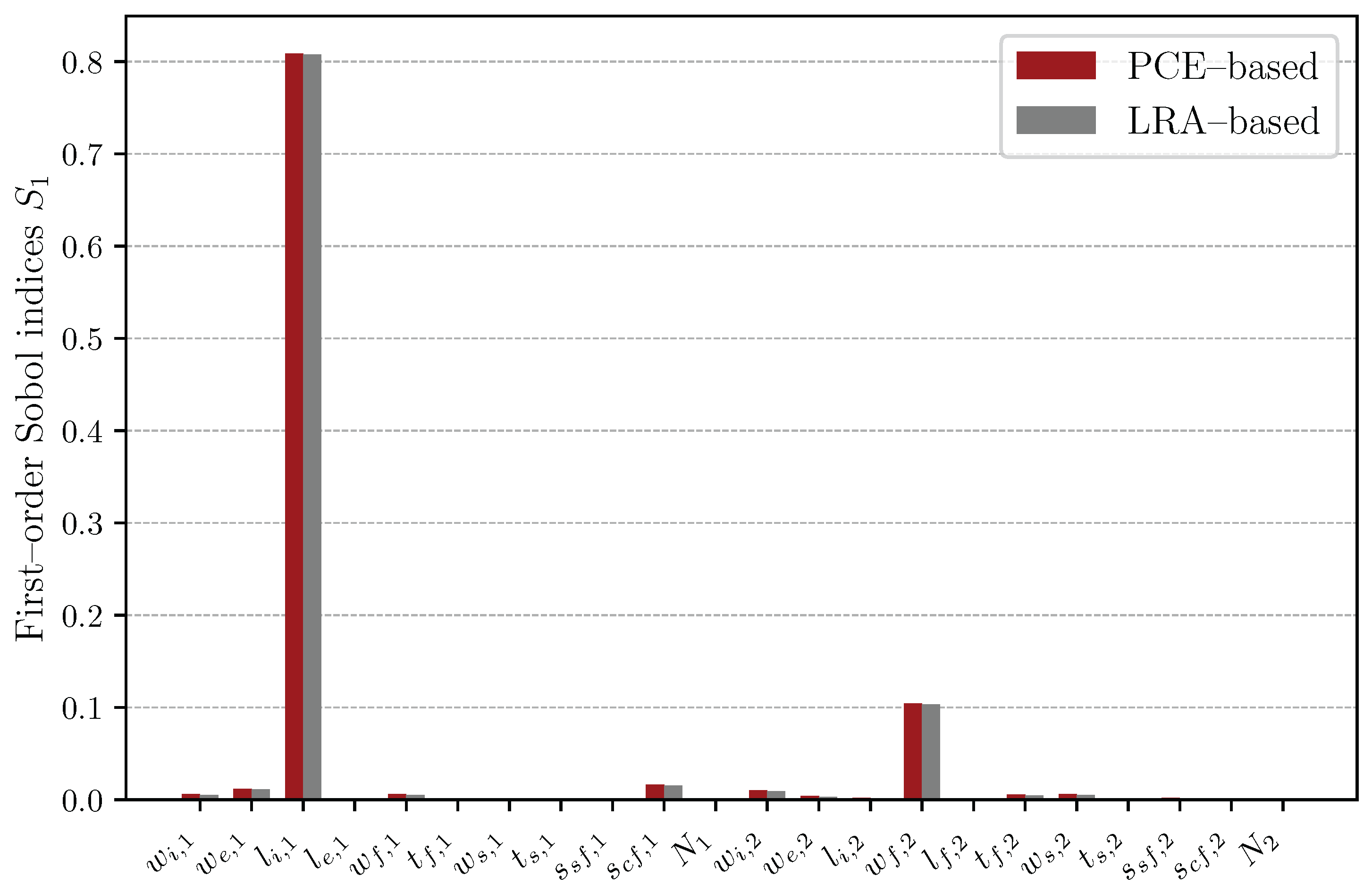
The first-order Sobol indices S 1 in Figure 8 convey a very similar picture. The primary coil interior length l i , 1 has S 1 = 0.809 , so its main effect alone explains most of the variance of the coupling coefficients. The width of the secondary ferrite w f , 2 contributes another S 1 = 0.104 , and the spacing between the primary coil and the ferrite has S 1 = 0.0163 . Thus, three physically interpretable parameters account for approximately 92.9 % of the variance.
When the S 1 indices are grouped by subsystems, the structure becomes even clearer. Summing the first-order indices of the primary coil dimensions ( w i , 1 , w e , 1 , l i , 1 and l e , 1 ) yields S 1 = 0.827 , representing the major influence on the coupling coefficients. Secondary ferrite parameters ( w f , 2 , l f , 2 , t f , 2 , s s f , 2 and s c f , 2 ) contribute S 1 = 0.113 , while all remaining parameters, primary and secondary ferrites, shielding, and windings, jointly contribute less than 5 % .
Adding all first-order indices yields S 1 = 0.986 , leaving 1.4 % for higher-order interactions between geometric variables. As expected, the sum of the total indices S T = 1.014 , which includes the interaction contributions, can be summed to values greater than one. This percentage S 1 is below one and S T is sightly above, which is exactly the regime described in the literature on sensibility analysis [42].
Comparing the total and first-order Sobol indices for each variable confirms that the most influential parameters act almost additively. For the interior length of the primary coil l i , 1 , the difference between the total and first-order indices is Δ S = S T S 1 0.815 0.809 = 0.006 , representing a small percentage of variance originating from interactions with this geometric variable. For the width for secondary ferrite w f , 2 , the corresponding difference is Δ S 0.110 0.104 = 0.006 , and for the spacing between the primary coil and the ferrite s c f , 1 , it is approximately Δ S 0.0014 . In contrast, some low-influence parameters present relatively larger ratios of ( S T S 1 ) / S T , but the absolute contribution to variance remains negligible because both total and first-order indices are close to zero.

4.3.2. Sensitivity of the Top Plane

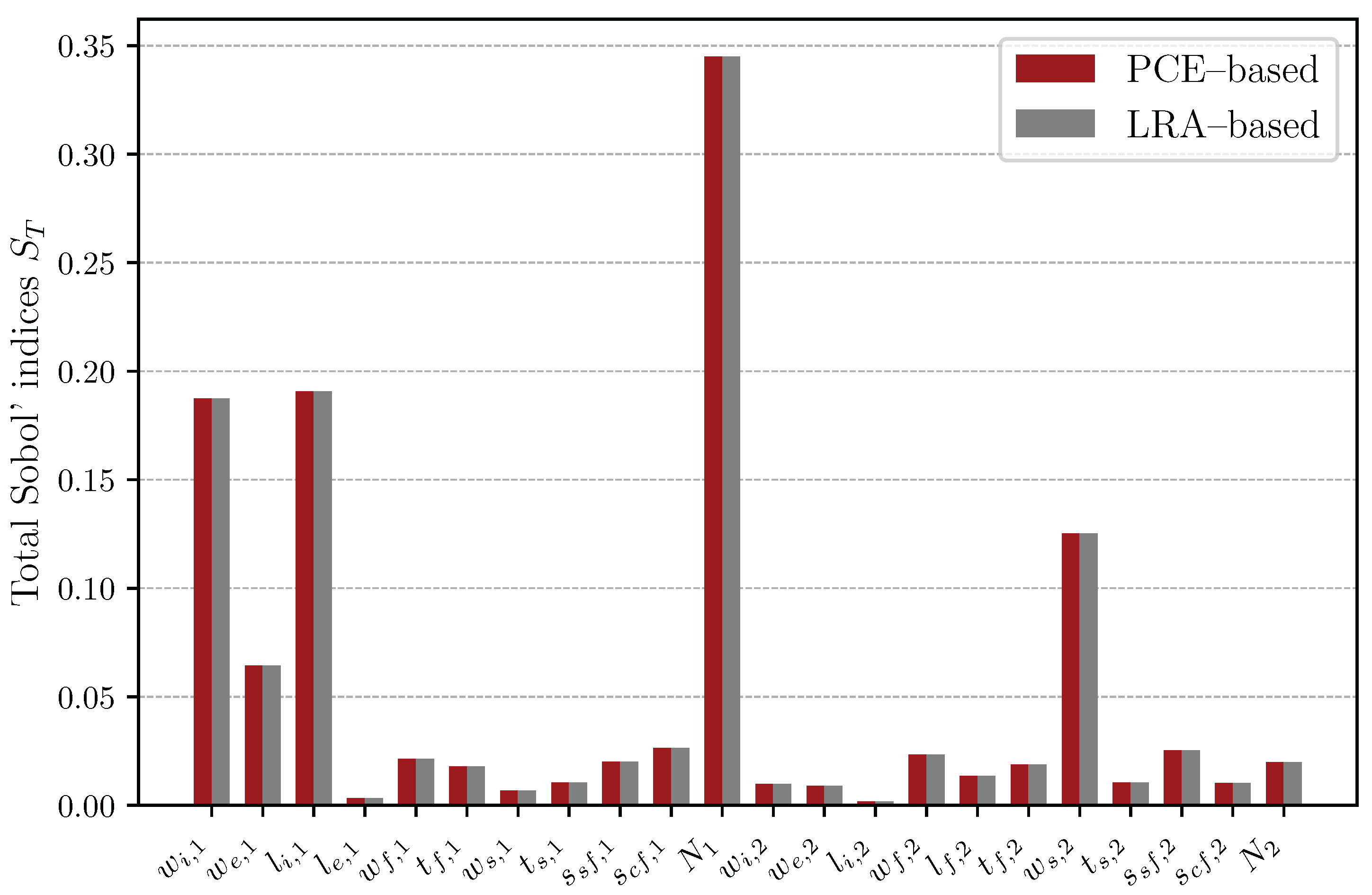
Figure 9 represents the total Sobol indices S T for the maximum magnitude of the complex magnetic flux density | B | t o p evaluated on the “top” plane, comparing PCE-based and LRA-based estimates. The magnetic flux on the “top” plane is mostly governed by primary-side excitation and coil geometry. The largest total index is associated with the primary number of windings N 1 , which corresponds to S T 0.345 . The interior width w i , 1 and length of the primary coil l i , 1 also play an major role in S t 0.188 and S T 0.191 , respectively.
Quantitatively, the total effect for these three parameters combined sums to S T ( N 1 ) + S T ( w i , 1 ) + S T ( l i , 1 ) 0.72 . Since the sum of all total indices is S T 1.16 , these three primary side quantities account for about 0.72 / 1.16 62 % of the total effect, with at least 72 % of the variance. A second group of influential parameters involves the secondary shield and ferrite geometries. The width of the secondary shield w s , 2 exhibits a substantial total index of S T 0.126 , while the width and thickness of the secondary ferrite and the spacing between the shield and the ferrite on the secondary side contribute with values in the range of 0.02 to 0.03 . In contrast, the remaining secondary side dimensions show only modest total effects of S T 0.02 . These results indicate that, on the secondary side, the maximum magnitude of the complex magnetic flux density max | B | t o p is mode sensitive to how the ferrite-shield assembly guides and contains the field rather than to fine details of the secondary winding.
When the total indices are grouped by physical subsystems, the dominance of the primary side becomes explicit. Summing over all geometrical parameters on the primary side yields a cumulative total effect S T 0.89 , whereas the corresponding sum for the dimensions on the secondary side yields S T 0.27 . As the total indices include interaction terms, these grouped sums do not represent disjoint fractions of variance, and their total S T 1.16 slightly exceeds the unit, indicating the presence of non-negligible interactions between design variables.
This pattern is entirely consistent with the underlying electromagnetic theory. The magnetic flux density generated by a coil is linked to the magnetic force, which is proportional to the product of the number of windings and the current. Since in the present study, the excitation current is fixed, variations in the number of windings of the primary coil directly influence the magnetomotive force and thus the local field levels. This strong dependence of the field on coil geometry and the number of windings is emphasised in recent work on IPT transmitter oil design [43].
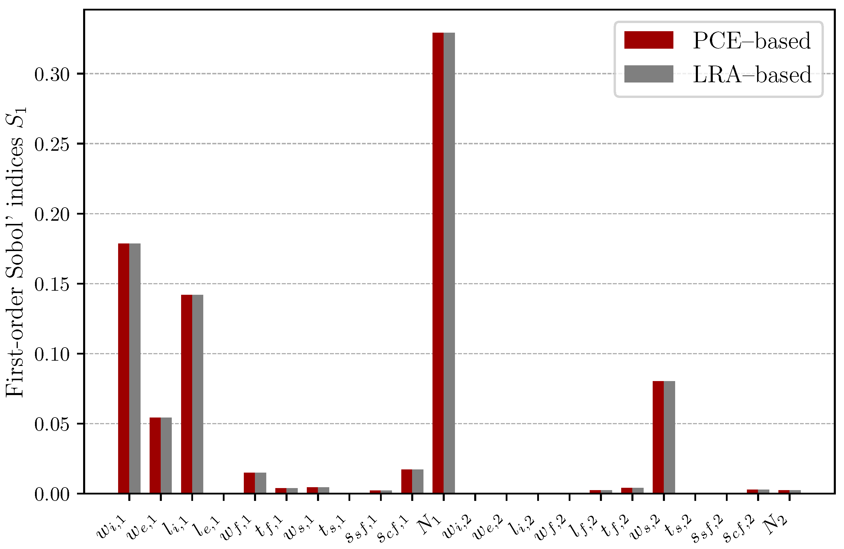
The first-order Sobol indices in Figure 10 represent the purely additive contribution of each geometrical parameters to the variance of the maximum magnitude of the complex magnetic flux density max | B | t o p evaluated on the top plane.
The ranking of the first-order indices confirms the strong dominance of the primary-side system. The largest first-order index is achieved by the number of windings of the primary coil N 1 , with S 1 0.33 . The interior dimensions of the primary coil are the next most influential, with the interior length l i , 1 and width w i , 1 corresponding to S 1 0.18 and S 1 0.14 , respectively. Together, they account for about 0.65 of the variance in max | B | t o p , which confirms the magnetomotive force on the primary winding.
At the level of individual variables, the leading contributors to max | B | t o p , w i , 1 , and l i , 1 remain predominantly additive, with their interaction shares modest compared to their main effects, such as S T S 1 0.016 and S T S 1 0.009 , respectively. In particular, the secondary shield width w s , 2 and a group of ferrite and spacing variables have total effect indices that are largely or almost entirely due to interactions, with S T S 1 accounting for approximately 80 to 100 % of their total contribution. Together, the variables with a S 1 0 but non-zero S T already accumulate S T 0.09 , which is not a negligible share. The structure and contribution of geometric variables are consistent with the physics of DIPT and the relevant literature.
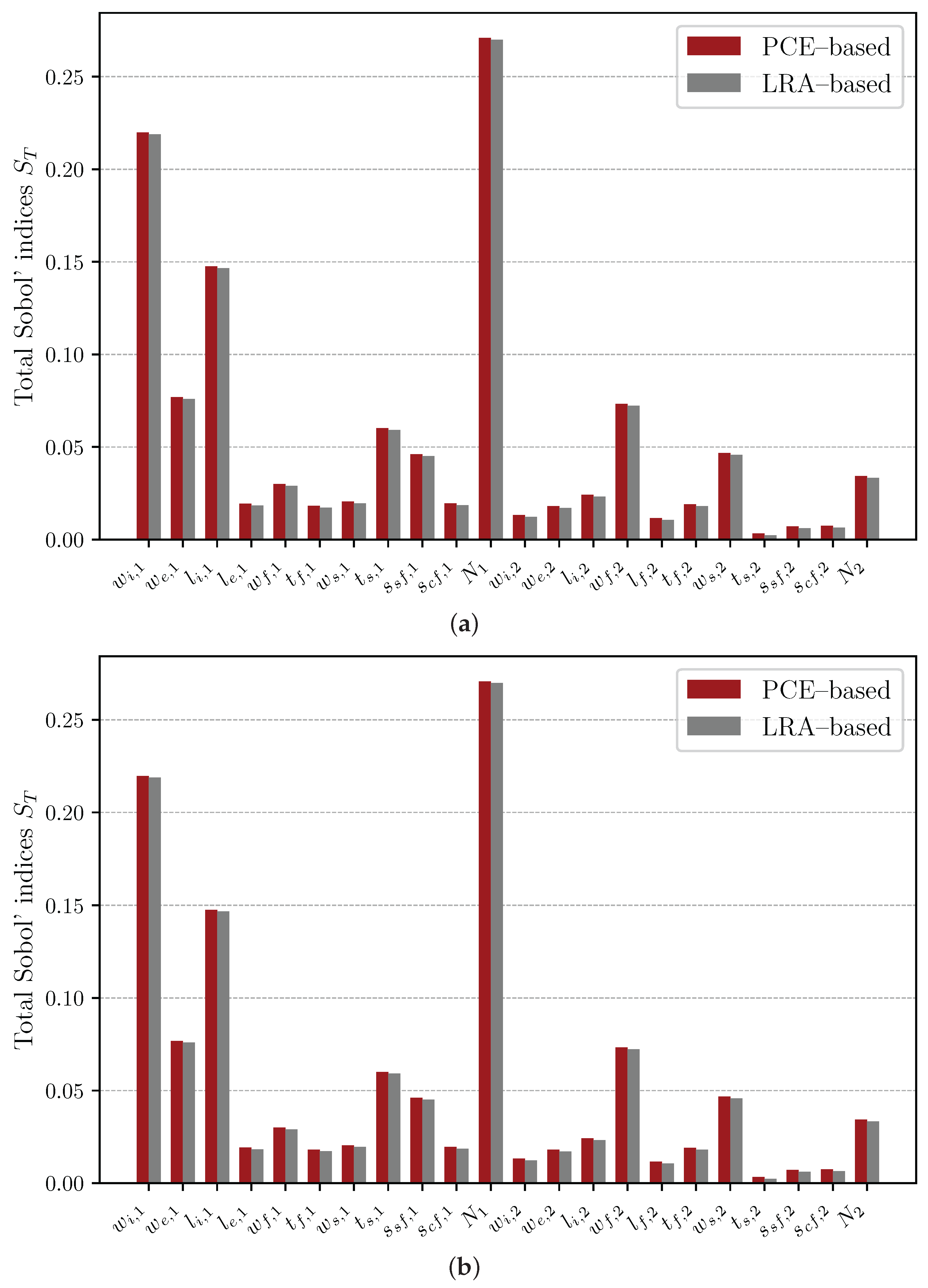
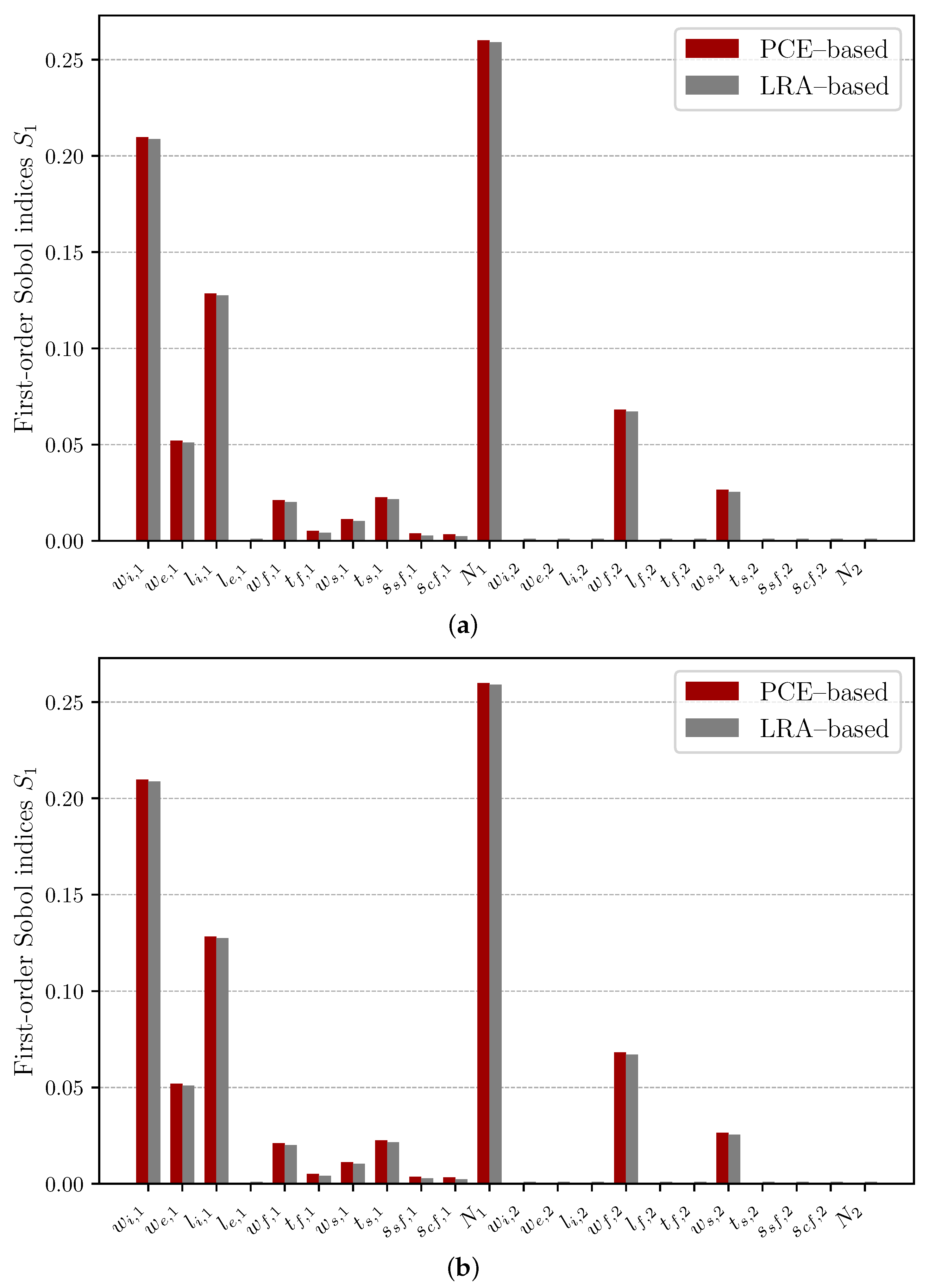
Figure 11 and Figure 12 show the total and first-order Sobol indices of the maximum magnitude of the complex magnetic flux density evaluated on the left (a) and right (b) control planes, respectively. As the coupler geometry and the nominal operation conditions are symmetric with respect to the longitudinal mid-plane of the system, the PCE- and LRA-based Sobol indices for the left and right planes are numerically indistinguishable. Each bar in the left plane lot has a counterpart of essentially identical height in the right plane plot. PCE and LRA estimates are visually coincident across all variables.

4.3.3. Sensitivity of the Lateral Control Planes

The total Sobol indices S T in Figure 11 capture both the main and interaction effects. The primary coil dimensions and number of windings remain the leading contributors, such the interior width, length, exterior width, and number of windings, with S T 0.22 , S T 0.15 , S T 0.08 and S T 0.27 , but several parameters that were negligible at first-order now display non-trivial effects. In particular, the primary shield thickness t s , 1 , the spacing between the primary shield and ferrite and between the coil and ferrite present very small first-order indices but S T values in the range of 0.02 to 0.06 . Similar patterns are found on the secondary side, where interior length, exterior width, ferrite length and thickness and number of windings have almost zero first-order indices but non-zero total indices, with S T values between approximately 0.01 and 0.03 .
The sum of all primary-side total indices is S T 0.93 , while the secondary side variables contribute with S T 0.26 , as the global sum is S T 1.19 , greater than the unit.
In terms of first-order indices S 1 , Figure 12 confirms that the lateral control planes are dominated by the same primary side drivers as the top plane but with a slightly different balance between coil windows and shielding effects. On both left and right planes, the largest first-order index is associated with the primary number of windings N 1 , with S T 0.26 , indicating that variations in the primary winding explain almost one-third of the variance of max | B | . The interior dimensions of the primary winding follow as the next most influential geometric parameters, with S 1 0.21 for the interior width w i , 1 and S 1 0.13 for the primary interior length l i , 1 . Taken together, these variables with N 1 already account for approximately 0.6 of the summed first-order indices. These variables represent the dominant additive design group that controls the field level in the lateral planes. Secondary side contributions at the first-order are appreciably smaller but not negligible. The secondary ferrite width w f , 2 exhibits S 1 0.07 , while the secondary shield width w s , 2 reaches S 1 0.03 . Other secondary dimensions and clearances are essentially negligible at the first-order, with S 1 values close to zero.
When the indices are grouped by sub-system, primary side parameters account for about S 1 0.72 , whereas the entire secondary side assembly contributes only with S 1 0.009 , reinforcing the conclusion that the lateral leakage field is primarily controlled by the excitation and geometry of the primary system, with the secondary ferrite and shield dimension exerting a subordinate influence.
Finally, the fact that both the total and first-order Sobol indices have been obtained from PCE and LRA surrogates, rather than from Monte Carlo simulations on the full Maxwell 3D model, is in line with recent work on surrogate-assisted analysis of DIPT and IPT systems [16].

4.3.4. Synthesis of Sensitivity Results

Overall, the Sobol indices obtained in this study characterise the relative importance of geometric variables for the nominal coupling condition (central position). In general terms, sensitivity analysis literature indicates that these indices depend on the distribution assumed for all input variables and may change when the statistics of other factors, such as misalignment, are fixed or modified.

4.4. Discussion and Implications for Optimisation

4.4.1. Identification of the Most Influential Geometric Parameters

The Sobol indices obtained in the previous section provide a coherent picture of the geometric parameters that govern both coupling and magnetic field levels. For the coupling coefficients k 11 , 2 and k 12 , 2 , the variance is mostly controlled by the interior length of the primary coil l i , 1 and, to a lesser extent, by the width of the secondary ferrite w f , 2 . Other primary coil dimensions and a small number of clearances between coils and ferrites contribute at a secondary level, while shield dimensions and the number of windings have almost negligible influence on the coupling. In contrast, the maximum magnitude of the complex magnetic flux density on the control planes is mainly driven by the primary-side excitation and window dimensions: the number of primary windings N 1 and the interior length and width of the primary coil ( l i , 1 and w i , 1 ) consistently exhibit the largest total and first-order indices for all three planes. Secondary-side ferrite and shield widths have moderate influence on the field levels, whereas most of the remaining dimensions act only through small interaction effects.
Taken together, these results indicate that a relatively small subset of design variables controls the key performance indicators of the DIPT coupler. The primary coil interior dimensions and the number of primary windings form a first group of drivers that simultaneously affect coupling and magnetic flux density. The secondary ferrite width, secondary shield width and a few selected clearances form a second group that has a more pronounced impact on field redistribution than on the dimensionless coupling factor. The remaining geometric parameters can be regarded as tertiary, as their total Sobol indices are at least one order of magnitude smaller and their contribution to the overall variance is marginal. This hierarchy of influences is central for interpreting the physical behaviour of the system and for understanding which dimensions are effectively controlling the responses explored in the optimisation stage.

4.4.2. Trade-Offs Between Coupling Efficiency and MF Exposure

The variables that appear simultaneously among the leading contributors to the variance of k 11 , 2 , k 12 , 2 and of the maximum magnetic flux density on the control planes encode structural couplings between these quantities. In particular, the interior length l i , 1 and width w i , 1 of the primary coil, together with the number of primary windings N 1 , have large Sobol indices for at least one coupling-related output and for all field-related outputs.
Conversely, several parameters play an asymmetric role across the two groups of outputs. The width of the secondary ferrite w f , 2 has a strong total effect on the coupling coefficients but only a modest contribution to the variance of the magnetic flux density, while the secondary shield width and certain spacings between ferrite and shield are much more influential for max | B | than for k 11 , 2 and k 12 , 2 .
In this context, the role of the Sobol indices is primarily interpretative rather than prescriptive. The sensitivity analysis identifies which parameters are expected to drive most of the variation in coupling and EMF exposure and therefore provides a natural framework to interpret the Pareto fronts obtained in Section 5 and to explain why certain design trends emerge across the optimal solutions.

5. Machine Learning Optimisation

For multi-objective optimisation problems, there is usually no single optimal solution but rather a set of trade-off solutions representing a compromise between objectives. Pareto fronts present a visual representation of the algorithm solutions, allowing the identification of candidate designs. All candidate designs, despite showing improvements in one parameter, show poor results for another parameter [44,45].
Among existing methods, the Non-Dominated Sorting Genetic Algorithm II (NSGA-II) is a widely applied algorithm for multi-objective optimisation. It incorporates a fast non-dominated sorting procedure to rank solutions into different levels and a mechanism to retain the best solutions between geometries. Using this type of algorithm, NGSA-II enhances computational efficiency and maintains a well-distributed Pareto front [45].

5.1. Optimisation Problem Formulation

The optimisation problem is expressed in terms of a geometric design vector g , which gathers all independent design variables and is restricted to the admissible set G . For any given geometry g , the operating conditions of the system are described by the misalignment and longitudinal position vector m = ( x , y , α ) D , which spans the prescribed ranges of lateral offset y, angular misalignment α and vehicle position x along the longitudinal axis. The surrogate is evaluated over this operating domain D and returns, for each pair ( g , m ) , the coupling coefficients k 11 , 2 ( g , m ) and k 12 , 2 ( g , m ) . From these response maps, the quantities k 11 , 2 min ( g ) , k 11 , 2 max ( g ) , k 12 , 2 min ( g ) and k 12 , 2 max ( g ) are defined as the minimum and maximum values attained by each coupling coefficient when m varies over D . The corresponding amplitudes
A 11 , 2 ( g ) = k 11 , 2 max ( g ) k 11 , 2 min ( g ) , A 12 , 2 ( g ) = k 12 , 2 max ( g ) k 12 , 2 min ( g ) ,
measure, for each geometry, the spread between the best and worst values of the coupling coefficients across all admissible misalignment and motion scenarios. The multi-objective optimisation problem is therefore constructed to identify designs g that, on the one hand, maximise the robustness of the coupling by increasing the minimum values k 11 , 2 min ( g ) and k 12 , 2 min ( g ) , and, on the other hand, reduce the sensitivity to misalignment by minimising the amplitudes A 11 , 2 ( g ) and A 12 , 2 ( g ) . These objectives are pursued under two classes of constraints: geometric constraints, which define the admissible design set G and ensure that the resulting coil, ferrite, and shielding dimensions are physically realisable, and MF exposure constraints, which impose that the magnetic flux density B p ( g , m ) on each control plane p { top , left , right } remains below the prescribed limit B lim = 27 μ T for all operating conditions m D .
The resulting geometric design problem can therefore be expressed as the following multi-objective optimisation problem, in which the decision vector g is chosen to maximise the minimum coupling coefficients and minimise their amplitude of variation over the operating domain D while satisfying the geometric and MF constraints:
max g k 11 , 2 min ( g ) , k 12 , 2 min ( g ) (16)
min g A 11 , 2 ( g ) , A 12 , 2 ( g ) (17)
subject to        g G , (18)
k 11 , 2 min ( g ) = min m D k 11 , 2 ( g , m ) , k 11 , 2 max ( g ) = max m D k 11 , 2 ( g , m ) , (19)
k 12 , 2 min ( g ) = min m D k 12 , 2 ( g , m ) , k 12 , 2 max ( g ) = max m D k 12 , 2 ( g , m ) , (20)
A 11 , 2 ( g ) = k 11 , 2 max ( g ) k 11 , 2 min ( g ) , A 12 , 2 ( g ) = k 12 , 2 max ( g ) k 12 , 2 min ( g ) , (21)
C ( g ) C max , (22)
max | B | p ( g , m ) 27 μ T , m D , p { top , left , right } . (23)
In addition to the multi-objective formulation in Equations (16)–(23), the geometric design vector g is restricted to an admissible set G defined by (i) simple bound constraints on each scalar design variable and (ii) a set of geometric consistency constraints that enforce a physically realisable coil–ferrite-shield arrangement on both the primary and secondary sides.
The bound constraints ensure that every design variable remains within the interval explored in the electromagnetic model and consistent with DoE limitations. Denoting generically by ξ j the j-th scalar component of g , one has
ξ j min ξ j ξ j max , j = 1 , , n g ,
where ξ j min and ξ j max are the lower and upper bounds reported in Table 6 for all geometric parameters.
Beyond these box constraints, additional inequalities are imposed to ensure that the coil windows are strictly contained within the corresponding ferrite and shield envelopes and that the difference between the width and length is sufficient to accommodate the prescribed number of turns, assuming an effective turn thickness of 5 mm per side [21]. The resulting geometric constraints can be written as
w i , 1 < w e , 1 w f , 1 w s , 1 ,
l i , 1 < l e , 1 ,
w e , 1 w i , 1 10 N 1 ,
l e , 1 l i , 1 10 N 1 ,
N 1 N ,
w i , 2 < w e , 2 w f , 2 w s , 2 ,
w e , 2 w i , 2 10 N 2 ,
l f , 2 l i , 2 10 N 2 ,
N 2 N
The chains of inequalities in (25)–(33) ensure that the interior coil windows ( w i , 1 , l i , 1 ) and ( w i , 2 , l i , 2 ) are strictly embedded within the corresponding ferrite and shield footprints, while the differences w e , k w i , k and l · , k l i , k provide sufficient space to accommodate N k the windings on both sides of the bounding, consistent with the adopted turn build model.
In addition to these geometric consistency requirements, an economic constraint is introduced to discourage excessively large and materially intensive designs that would provide only marginal improvements in coupling performance. A scalar material index C ( g ) is defined as
C ( g ) = k = 1 2 w s , k l s , k t s , k + w f , k l f , k t f , k , k { 1 , 2 }
which is proportional to the total shield and ferrite volumes on the primary ( k = 1 ) and secondary ( k = 2 ) sides. The admissible design set is further restricted by
C ( g ) C max ,
where C max denotes the maximum acceptable material index based on cost, mass and packaging considerations. This additional inequality, see (22), prevents the optimiser from simply enlarging the material dimensions to achieve robustness against misalignment at the expense of an impractical increase in material usage.

5.2. Random Forest Surrogate Error Metrics

The error metrics in Table 9 indicate that the random forest surrogates reproduce the coupling coefficients with very considerable accuracy.
For k 11 , 2 and k 12 , 2 , the combination of high R 2 and relatively small train–test degradation is consistent with the ability of ensemble tree methods to approximate complex non-linear mappings while maintaining good generalisation when a sufficient number of trees and samples are available. These results suggest that the random forest models are capable of capturing the main geometric trends of the coupling coefficients over the design space and are therefore suitable for use as inexpensive surrogates within the NSGA-II optimisation process.
For the maximum magnetic flux density, the performance is more heterogeneous. The lateral control planes exhibit strong predictive quality, with R test 2 = 0.87 0.88 and RMSE test below 3 μ T, indicating that the surrogates explain most of the variance in max | B | left and max | B | right . In contrast, the top-plane surrogate achieves a markedly lower generalisation score of R test 2 = 0.61 , and the corresponding test RMSE is approximately three times greater than for the lateral planes, signalling a more challenging response surface and a higher level of unexplained variability. In the context of the present optimisation study, these figures imply that random forest models provide reliable guidance for coupling-related objectives and for lateral field constraints, whereas predictions of max | B | top should be interpreted with more caution.

5.3. Candidate Designs and Pareto Fronts

The numerical values in Table 10 summarise the objectives associated with the initial geometry and with four representative NSGA-II candidates. For all candidates, the worst-case coupling coefficients k 11 , 2 min and k 12 , 2 min are less negative than in the initial design, indicating an improvement in robustness with respect to misalignment. Candidate 3 attains the highest primary-side minimum ( k 11 , 2 min = 0.0379 ), but this comes at the price of the largest amplitudes A 11 , 2 and A 12 , 2 among the candidates, reflecting stronger variation in the coupling coefficients across the operating domain D . Candidate 1 is the most favourable in terms of the primary amplitude A 11 , 2 , while candidate 2 exhibits the lowest secondary amplitude A 12 , 2 , with both designs achieving noticeable reductions relative to the initial geometry. Candidate 4 sits between these extremes, combining improved minimum couplings on both sides with moderate amplitudes, and can therefore be interpreted as a compromise solution between robustness and sensitivity.
These tendencies are consistent with the Pareto diagrams in Figure 13, Figure 14, Figure 15 and Figure 16, which display the population of non-dominated solutions obtained with NSGA-II and the positions of the initial design and of candidates 1–4. In Figure 13, the most desirable region corresponds to the lower-left area, where k 11 , 2 min and A 11 , 2 are high and low, respectively. The initial design is located towards the upper-right part of the front, confirming its relatively low robustness and large primary amplitude. Moving along the front towards lower A 11 , 2 leads to candidate 1, which substantially reduces the spread of k 11 , 2 at the cost of a more modest improvement in the minimum value. In contrast, candidate 3 lies closer to the region of very high k 11 , 2 min , but with a larger A 11 , 2 , illustrating the compromise between maximising the worst-case coupling and controlling its variation. An analogous interpretation applies to Figure 14 for the secondary-side objectives, where candidate 2 clearly favours a reduction in A 12 , 2 , candidate 3 prioritises k 12 , 2 min , and candidate 4 appears near a knee region that balances both criteria.
The interaction between primary and secondary robustness is further clarified in Figure 15, which plots k 11 , 2 min ( g ) against k 12 , 2 min ( g ) . The initial design occupies a corner of the diagram where both minima are relatively low, while the NSGA-II front spans a band of solutions in which improvements on one side tend to degrade the other. Candidate 3 is displaced towards the region of high primary robustness but exhibits only moderate gains on the secondary side, whereas candidate 2 behaves in the opposite manner. Candidate 4 is located near the centre of the front, showing simultaneous, though not extreme, improvements in both minimal values. Finally, Figure 16 reveals that the amplitudes A 11 , 2 and A 12 , 2 are also correlated: designs that strongly reduce the variation of one coupling coefficient often increase, or only slightly decrease, the variation of the other. Candidate 1 reduces A 11 , 2 while maintaining A 12 , 2 at a level close to the initial value, candidate 2 is particularly effective in reducing A 12 , 2 , and candidate 4 again offers a balanced compromise, with both amplitudes below those of the initial geometry. These observations guided the selection of the candidates for detailed finite-element validation in the subsequent sections.

5.4. Response Surfaces of Initial and Optimised Design

The response surfaces of the coupling coefficient k 11 , 2 provide a compact visual representation of how the primary–secondary coupling evolves with vehicle position and misalignment and are therefore useful to assess the impact of the geometric optimisation. Figure 17 and Figure 18 compare the lateral response surfaces k 11 , 2 ( x , y ) for the initial geometry and for candidate design 3, respectively.
In the initial configuration (Figure 17), the coupling exhibits a relatively localised peak around the central region of the longitudinal axis and near-zero lateral offset, followed by a rapid decay as x increases or as the vehicle moves away from the alignment line. Negative or near-zero values appear as soon as the vehicle crosses the end of the primary coils, indicating that the system quickly loses effective coupling outside a narrow operating window.
The optimised geometry, represented in Figure 18, yields a noticeably broader level of high k 11 , 2 values along the longitudinal direction for a wider range of lateral offsets. The peak coupling level is increased and the transition towards lower values is more gradual, particularly for moderate lateral misalignments. This behaviour is consistent with the NSGA-II objectives of improving the minimum coupling coefficient and reducing its sensitivity to lateral displacement, confirming that candidate 3 provides a more robust lateral response than the initial design.
A similar trend is observed when the coupling coefficient is plotted against the longitudinal position and angular misalignment, k 11 , 2 ( x , α ) , in Figure 19 and Figure 20. For the initial design, the response surface shows a pronounced dependence on α in the vicinity of the alignment condition: small angular deviations around α = 0 already lead to a significant reduction in k 11 , 2 , and the coupling rapidly decreases to very low values as the vehicle leaves the region above the primary coils. Figure 20 indicates that for the optimised geometry of candidate 3, the high-coupling ridge around α = 0 becomes both higher and wider.
This indicates that the system maintains stronger coupling for a larger range of angular misalignments and longitudinal positions. The surface is less smooth and the gradients with respect to α are maintained, which is consistent with the improved minimum coupling and larger robustness indices reported earlier. Overall, the comparison of the response surfaces confirms that candidate 3 not only increases the peak values of k 11 , 2 but also flattens the response with respect to both lateral and angular misalignment, thereby providing a more stable and practically usable charging performance along the dynamic charging lane.

5.5. Magnetic Flux Density on the Control Planes

The profiles of the maximum magnitude of the complex magnetic flux density on the control planes provide a direct assessment of MF exposure for both the initial and the optimised geometries. The angular-misalignment plots in Figure 21, Figure 22 and Figure 23 show max | B | top ( α ) , max | B | left ( α ) and max | B | right ( α ) at the YZ plane corresponding to the peak coupling, respectively. For the initial design, all three planes exhibit nearly flat but high levels, with max | B | top around 73 μ T and the lateral planes around 46– 47 μ T over the whole range 0 α 20 , which substantially exceeds the adopted exposure limit of 27 μ T .
In contrast, candidate design 3 maintains field levels close to 22 μ T on the top plane and approximately 18 μ T on the left and right planes, with only very small variations as α increases. The optimised geometry therefore reduces the angular-misalignment field levels by a factor of about three on the top plane and by a factor of about two and a half on the lateral planes while also providing almost perfectly flat profiles, which is consistent with the robustness objective of the optimisation problem.
A similar behaviour is observed for lateral misalignment in Figure 24 and Figure 25, which display max | B | left ( y ) and max | B | right ( y ) as functions of the offset 0 y 300 mm . For the initial design, the lateral field on both planes remains in the range 45– 47 μ T , showing a modest dependence on y but persistently exceeding the exposure limit across the whole interval. Candidate 3 again confines the field to approximately 18– 19 μ T , largely independent of y and comfortably below the 27 μ T threshold. Taken together, the angular and lateral profiles demonstrate that the optimised geometry simultaneously increases the coupling coefficients (Section 5.3) and achieves a substantial and uniform reduction of the magnetic flux density on all control planes, thereby fulfilling the MF-compliance constraint with a significant safety margin.

5.6. Comparison of the Initial and the Optimised Design

The quantitative comparison in Table 10 shows that candidate design 3 achieves a systematic improvement of the coupling coefficients with respect to the initial geometry. The worst-case primary coupling increases from k 11 , 2 min = 0.0618 to k 11 , 2 min = 0.0379 , while the corresponding maximum rises from 0.3172 to 0.3566 , so that both the lower and upper bounds of k 11 , 2 are shifted towards more favourable values. On the secondary side, k 12 , 2 min improves from 0.0873 to 0.0550 and k 12 , 2 max from 0.3090 to 0.3986 . These variations correspond to increments of approximately 0.02 0.09 in the coupling coefficients across the operating domain, confirming that candidate 3 provides stronger coupling for both coils in almost all operating conditions. This enhancement is obtained at the expense of a moderate increase in the amplitudes A 11 , 2 and A 12 , 2 , which reflects the higher peak values attained by the optimised design.
The angular and lateral profiles, together with the response surfaces (Figure 17, Figure 18, Figure 19 and Figure 20), confirm that the coupling of candidate 3 is not only higher on average but also more robust to misalignment. Along both the angular coordinate α and the lateral offset y, the k 11 , 2 curves of candidate 3 are consistently above those of the initial design over a wide portion of the admissible range, and the transitions between the central alignment region and the misaligned configurations become smoother. In particular, the level of high coupling extends over a larger interval of longitudinal positions x and misalignment values, so the optimised geometry maintains useful coupling for a broader set of driving trajectories.
The magnetic flux density profiles in Figure 21, Figure 22, Figure 23, Figure 24 and Figure 25 indicate that these gains in coupling are obtained without a detrimental increase in the field levels on the control planes. For all three planes and for both angular and lateral misalignments, the max | B | curves of candidate 3 remain of the same order of magnitude as those of the initial design, and the peaks are constrained by the exposure limit imposed in the optimisation problem. Taken together, the results demonstrate that candidate 3 represents a genuinely improved geometry: it delivers higher and more robust coupling coefficients over the operating domain while preserving MF exposure within the prescribed bounds.

6. Conclusions and Future Work

The present work has addressed the geometric design of a DIPT coupler for two-wheeled electric vehicles, with particular emphasis on maintaining robust electromagnetic coupling under misalignment while satisfying MF exposure constraints derived from current automotive standards. This work has combined finite-element modelling, surrogate modelling and global sensitivity analysis, and multi-objective optimisation into a single workflow, implemented using an Ansys Maxwell 3D model and advanced optimisation and GSA tools.

6.1. Summary of Key Findings

The three-dimensional finite element model developed in this work captures the dominant electromagnetic behaviour of shielded rectangular DIPT couplers under realistic longitudinal movement, lateral, and angular misalignments. A compact parametrisation of coil, ferrite, and shield geometries enables systematic exploration of designs consistent with the packaging constraints of an e-motorcycle. The use of temperature-dependent ferrite behaviour and realistic conductor and excitation assumptions for SS-compensated operation at 85 kHz supports physically consistent predictions of coupling and magnetic field emission over the investigated domain.
The finite element results show that the baseline design provides adequate coupling near alignment but exceeds the adopted magnetic field reference levels on the top and lateral control planes over parts of the misalignment envelope, with leakage peaks near the primary end regions and under combined offsets. Full model re-evaluation of a representative non-dominated sorting genetic algorithm design confirms that coordinated geometric adjustments can simultaneously improve coupling robustness and reduce exposure. Sparse PCE and canonical LRA reproduce the finite element responses with accuracy adequate for global sensitivity analysis, and their Sobol indices consistently identify primary coil dimensions and number of windings as the principal drivers of both coupling and the control plane’s magnetic field. Random forest surrogates trained on the joint geometry and misalignment dataset enable multi-objective optimisation that exposes trade-offs among worst-case coupling, robustness, and magnetic field constraints, and selected solutions are confirmed by finite element re-simulation, supporting the combined workflow of surrogate-based screening and optimisation for exposure-constrained coupler design.

6.2. Limitations of the Present Work

This work considers a single coupler topology and vehicle integration, so sensitivity patterns and optimal geometries may not transfer to alternative shapes, multi-coil arrangements, or different packaging constraints.
Surrogate accuracy degrades in sparsely sampled regions. PCE assumes smooth input dependence and is sensitive to distribution and truncation choices, with lower fidelity observed for the top control plane surrogate. The optimisation is quasi-static and omits losses, thermal constraints, power electronics, and manufacturing tolerances or material variability. Although the operating domain includes the longitudinal position x, this study is performed as a sequence of pose evaluations. Therefore, vehicle speed and the associated time evolution of ( x , y , α ) are not modelled.

6.3. Recommendations for Future Work

Future research should extend the electromagnetic model to include conductor, ferrite, and shield losses, coupled electro-thermal simulations, and thermal–mechanical constraints. This would enable multi-objective optimisation that jointly targets coupling performance, MF exposure, and temperature rise under realistic operating conditions. It should couple the parameterised electromagnetic responses with vehicle kinematics and speed profiles to quantify time-domain coupling stability and MF exposure during driving, including correlated trajectories derived from measured data and closed-loop power-transfer control.
Surrogate and sensitivity workflows should be expanded using alternative regressors for strongly localised responses and by treating misalignment as a stochastic input. The framework should be validated experimentally using prototypes tested under controlled misalignments to calibrate models and account for tolerances, material variability, and environmental effects.

Supplementary Materials

The following supporting information can be downloaded at: https://www.mdpi.com/article/10.3390/en19061456/s1, Figure S1: Global and relative coordinate systems used in finite-element modelling. Figure S2: Control planes over the finite–element model. Table S1: Geometric parametrisation of the primary coil (total volume and removed volume). Table S2: Geometric parametrisation of the primary ferrite. Table S3: Geometric parametrisation of the primary shield. Table S4: Geometric parametrisation of the secondary coil (total volume and removed volume). Table S5: Geometric parametrisation of the secondary ferrite. Table S6: Geometric parametrisation of the secondary shielding.

Author Contributions

Conceptualization, M.L., R.M.M.P. and A.J.C.P.; Methodology, M.L.; Validation, M.L.; Formal analysis, R.M.M.P. and A.J.C.P.; Investigation, M.L.; Writing—original draft, M.L.; Writing—review & editing, R.M.M.P. and A.J.C.P.; Supervision, R.M.M.P. and A.J.C.P. All authors have read and agreed to the published version of the manuscript.

Funding

This research received no external funding.

Institutional Review Board Statement

Not applicable.

Informed Consent Statement

Not applicable.

Data Availability Statement

The original contributions presented in this study are included in the article. Further inquiries can be directed to the corresponding author.

Conflicts of Interest

The authors declare no conflicts of interest.

References

  1. Zio, E. Monte Carlo Simulation: The Method. In The Monte Carlo Simulation Method for System Reliability and Risk Analysis; Springer Series in Reliability Engineering; Springer: London, UK, 2013; pp. 19–58. [Google Scholar] [CrossRef] [Scilit]
  2. Forrester, A.I.J.; Sóbester, A.; Keane, A.J. Engineering Design via Surrogate Modelling: A Practical Guide, 1st ed.; Wiley: Hoboken, NJ, USA, 2008. [Google Scholar] [CrossRef] [Scilit]
  3. Lataniotis, C.; Wicaksono, D.; Marelli, S.; Sudret, B. UQLab User Manual—Kriging (Gaussian Process Modeling); Technical Report; Chair of Risk, Safety and Uncertainty Quantification, ETH Zurich: Zurich, Switzerland, 2024. [Google Scholar]
  4. Marelli, S.; Lüthen, N.; Sudret, B. UQLab User Manual—Polynomial Chaos Expansions; Technical Report; Chair of Risk, Safety and Uncertainty Quantification, ETH Zurich: Zurich, Switzerland, 2024. [Google Scholar]
  5. Konakli, K.; Mylonas, C.; Marelli, S.; Sudret, B. UQLab User Manual—Canonical Low-Rank Approximations; Technical Report; Chair of Risk, Safety and Uncertainty Quantification, ETH Zurich: Zurich, Switzerland, 2024. [Google Scholar]
  6. Konakli, K.; Sudret, B. Polynomial meta-models with canonical low-rank approximations: Numerical insights and comparison to sparse polynomial chaos expansions. J. Comput. Phys. 2016, 321, 1144–1169. [Google Scholar] [CrossRef] [Scilit]
  7. Chevreuil, M.; Lebrun, R.; Nouy, A.; Rai, P. A Least-Squares Method for Sparse Low Rank Approximation of Multivariate Functions. SIAM/ASA J. Uncertain. Quantif. 2015, 3, 897–921. [Google Scholar] [CrossRef] [Scilit]
  8. Sudret, B. Global sensitivity analysis using polynomial chaos expansions. Reliab. Eng. Syst. Saf. 2008, 93, 964–979. [Google Scholar] [CrossRef] [Scilit]
  9. Marelli, S.; Lamas, C.; Konakli, K.; Mylonas, C.; Wiederkehr, P.; Sudret, B. UQLab User Manual—Sensitivity Analysis; Technical Report; Chair of Risk, Safety and Uncertainty Quantification, ETH Zurich: Zurich, Switzerland, 2024. [Google Scholar]
  10. Xiu, D. Numerical Methods for Stochastic Computations: A Spectral Method Approach; Princeton University Press: Princeton, NJ, USA, 2010. [Google Scholar] [CrossRef] [Scilit]
  11. Blatman, G.; Sudret, B. Adaptive sparse polynomial chaos expansion based on least angle regression. J. Comput. Phys. 2011, 230, 2345–2367. [Google Scholar] [CrossRef] [Scilit]
  12. Blatman, G. Adaptive Sparse Polynomial Chaos Expansions for Uncertainty Propagation and Sensitivity Analysis. Ph.D. Thesis, Université Blaise Pascal, Clermont-Ferrand, France, 2009. [Google Scholar]
  13. Breiman, L. Random Forests. Mach. Learn. 2001, 45, 5–32. [Google Scholar] [CrossRef] [Scilit]
  14. Biau, G.; Scornet, E. A random forest guided tour. TEST 2016, 25, 197–227. [Google Scholar] [CrossRef] [Scilit]
  15. Saltelli, A. (Ed.) Global Sensitivity Analysis: The Primer; John Wiley: Chichester, UK; Hoboken, NJ, USA, 2008. [Google Scholar] [CrossRef] [Scilit]
  16. Pei, Y. Design and Optimization of Inductive Power Transfer Systems by Metamodeling Techniques. Ph.D. Thesis, Université Paris-Saclay, Gif-sur-Yvette, France, 2023. [Google Scholar]
  17. Lagouanelle, P.; Boulitrop, C.; Pichon, L.; Freschi, F.; Lambert, M. Gradient-based metamodel optimization for the design of 3F3 Ferrites Core in a WPT system. In Proceedings of the 2023 24th International Conference on the Computation of Electromagnetic Fields (COMPUMAG), Kyoto, Japan, 22–26 May 2023. [Google Scholar]
  18. Ansys Maxwell Brochure; Ansys: Canonsburg, PA, USA, 2011.
  19. Nimri, R.M.; Kamineni, A.; Zane, R. A Modular Pad Design compatible with SAE J2954 for Dynamic Inductive Power Transfer. In Proceedings of the 2020 IEEE PELS Workshop on Emerging Technologies: Wireless Power Transfer (WoW), Seoul, Republic of Korea, 15–19 November 2020; pp. 45–49. [Google Scholar] [CrossRef] [Scilit]
  20. Afonso, J.A.; Duarte, H.G.; Cardoso, L.A.L.; Monteiro, V.; Afonso, J.L. Wireless Communication and Management System for E-Bike Dynamic Inductive Power Transfer Lanes. Electronics 2020, 9, 1485. [Google Scholar] [CrossRef] [Scilit]
  21. SAE J 2954; Wireless Power Transfer for Light-Duty Plug-in/Electric Vehicles and Alignment Methodology. SAE International: Warrendale, PA, USA, 2024.
  22. IEC 61980-3; Electric Vehicle Wireless Power Transfer (WPT) Systems—Part 3: Specific Requirements for Magnetic Field Wireless Power Transfer Systems. International Electrotechnical Commission: Geneva, Switzerland, 2022.
  23. IEEE/IEC 63184-2025; Assessment Methods of the Human Exposure to Electric and Magnetic Fields from Wireless Power Transfer Systems—Models, Instrumentation, Measurement and Computational Methods and Procedures (Frequency Range of 3 kHz to 30 MHz). IEEE Standards Association: Piscataway, NJ, USA, 2025.
  24. High Frequency Litz Wire—Product Program and Technical Data; Elektrisola: Reichshof-Eckenhagen, Germany, 2025.
  25. IEC 60317-11; Specifications for Particular Types of Winding Wires—Part 11: Bunched Solderable Polyurethane Enamelled Round Copper Wires, Class 130, with Silk Covering. International Electrotechnical Commission: Geneva, Switzerland, 2005. [CrossRef] [Scilit]
  26. Sullivan, C.R.; Zhang, R.Y. Simplified design method for litz wire. In Proceedings of the 2014 IEEE Applied Power Electronics Conference and Exposition—APEC 2014, Fort Worth, TX, USA, 16–20 March 2014; pp. 2667–2674. [Google Scholar] [CrossRef] [Scilit]
  27. Litz Wire Details; Elektrisola: Reichshof-Eckenhagen, Germany, 2025.
  28. TDK Power Ferrite Material PC47, PC90 and PC95; TDK: Chuo, Japan, 2011.
  29. IEC 61980-1; Electric Vehicle Wireless Power Transfer (WPT) Systems—Part 1: General Requirements. International Electrotechnical Commission: Geneva, Switzerland, 2020.
  30. Kis, P. Parameter identification of Jiles–Atherton model with nonlinear least-square method. Phys. B Condens. Matter 2004, 343, 59–64. [Google Scholar] [CrossRef] [Scilit]
  31. Stucky, P.; Lord, W. Skin Depth Considerations in Eddy Current NDT. In Review of Progress in Quantitative Nondestructive Evaluation; Thompson, D.O., Chimenti, D.E., Eds.; Springer: Boston, MA, USA, 1992; pp. 299–306. [Google Scholar] [CrossRef] [Scilit]
  32. Desai, P.D.; James, H.M.; Ho, C.Y. Electrical Resistivity of Aluminum and Manganese. J. Phys. Chem. Ref. Data 1984, 13, 1131–1172. [Google Scholar] [CrossRef] [Scilit]
  33. International Commission on Non-Ionizing Radiation Protection. Guidelines for Limiting Exposure to Time-varying Electric and Magnetic Fields (1 Hz to 100 kHz). Health Phys. 2010, 99, 818–836. [Google Scholar] [CrossRef] [Scilit] [PubMed]
  34. C95.1-2019; IEEE Standard for Safety Levels with Respect to Human Exposure to Electric, Magnetic, and Electromagnetic Fields, 0 Hz to 300 GHz. IEEE Standards Association: Piscataway, NJ, USA, 2019. [CrossRef] [Scilit]
  35. Campi, T.; Cruciani, S.; Maradei, F.; Feliziani, M. Two-Coil Receiver for Electrical Vehicles in Dynamic Wireless Power Transfer. Energies 2021, 14, 7790. [Google Scholar] [CrossRef] [Scilit]
  36. Maxwell(R) Help Release 2025 R2; Ansys Inc.: Canonsburg, PA, USA, 2025.
  37. Marelli, S.; Sudret, B. UQLab: A Framework for Uncertainty Quantification in Matlab. In Proceedings of the Vulnerability, Uncertainty, and Risk, Liverpool, UK, 13–16 June 2014; pp. 2554–2563. [Google Scholar] [CrossRef] [Scilit]
  38. Leng, Y.; Luo, D.; Li, Z.; Yu, F. Coupling coefficient calculation and optimization of positive rectangular series coils in wireless power transfer systems. Heliyon 2023, 9, e21121. [Google Scholar] [CrossRef] [Scilit] [PubMed]
  39. Yang, S.C.; He, H.; Yan, X.Y.; Chen, Y.H.; Hua, Y.; Cao, Y.G.; Li, J.; Li, H.H.; Yin, S. Segmental Track Analysis in Dynamic Wireless Power Transfer. Energies 2019, 12, 3875. [Google Scholar] [CrossRef] [Scilit]
  40. Bareli, S.; Geri, L.; Nikulshin, Y.; Nahum, O.E.; Hadas, Y.; Yeshurun, Y.; Yaniv, E.; Wolfus, S. Effect of Coil Dimensions on Dynamic Wireless Power Transfer for Electric Vehicles. TechRxiv 2021. [Google Scholar] [CrossRef] [Scilit]
  41. Bensetti, M.; Kadem, K.; Pei, Y.; Le Bihan, Y.; Labouré, E.; Pichon, L. Parametric Optimization of Ferrite Structure Used for Dynamic Wireless Power Transfer for 3 kW Electric Vehicle. Energies 2023, 16, 5439. [Google Scholar] [CrossRef] [Scilit]
  42. Zimmermann, J.; Altenkirch, R.; Van Rienen, U. Numerical study on the effect of capacitively coupled electrical stimulation on biological cells considering model uncertainties. Sci. Rep. 2022, 12, 4744. [Google Scholar] [CrossRef] [Scilit] [PubMed]
  43. Prosen, N.; Milanovič, M.; Domajnko, J. Magnetic Flux Density Measurement Platform for an Inductive Wireless Power Transmitter Coil Design. Sensors 2022, 22, 479. [Google Scholar] [CrossRef] [Scilit] [PubMed]
  44. Buck, V.D.; López, C.A.M.; Nimmegeers, P.; Hashem, I.; Impe, J.V. Multi-objective optimisation of chemical processes via improved genetic algorithms: A novel trade-off and termination criterion. In Computer Aided Chemical Engineering; Elsevier: Amsterdam, The Netherlands, 2019; Volume 46, pp. 613–618. [Google Scholar] [CrossRef] [Scilit]
  45. Keller, A.A. Multi-Objective Optimization in Theory and Practice II: Metaheuristic Algorithms; Bentham Science Publisher: Sharjah, United Arab Emirates, 2019. [Google Scholar]
Figure 1. Workflow overview.
Energies 19 01456 g001
Figure 2. Topology of the proposed optimisation model consisting of a shielded coupling.
Energies 19 01456 g002
Figure 3. Schematic representation of the geometry dimensions. Top and side view of the: (a) Primary coil. (b) Secondary coil.
Energies 19 01456 g003
Figure 4. Classification of movement misalignment in e-motorcycles: (a) Lateral (y-axis). (b) Rotation (x-axis).
Energies 19 01456 g004
Figure 5. Evolution of the leave-one-out error E LOO along the LARS iterations for the sparse PCE surrogates of: (a) Coupling coefficients k 11 , 2 and k 12 , 2 . (b) Maximum magnetic flux density on the top control plane max | B | top . (c) Maximum magnetic flux density on the left control plane max | B | left . (d) Maximum magnetic flux density on the right control plane max | B | right .
Energies 19 01456 g005
Figure 6. Comparison of estimated probability density functions by polynomial chaos expansions surrogate and finite element method for: (a) k 11 , 2 and k 12 , 2 , (b) max | B | t o p , (c) max | B | l e f t , (d) max | B | r i g h t .
Energies 19 01456 g006
Figure 7. Total Sobol indices S T for the coupling coefficients k 11 , 2 and k 12 , 2 for the DIPT coupler, comparing PCE-based and LRA-based estimates for all geometric design variables under nominal misalignment.
Energies 19 01456 g007
Figure 8. First-order Sobol indices S T for the coupling coefficients k 11 , 2 and k 12 , 2 for the DIPT coupler, comparing PCE-based and LRA-based estimates for all geometric design variables under nominal misalignment.
Energies 19 01456 g008
Figure 9. Total Sobol indices S T for the maximum magnitude of the complex magnetic flux density max | B | t o p evaluated on the top plane, comparing PCE-based and LRA-based estimates for all geometric design variables under nominal misalignment.
Energies 19 01456 g009
Figure 10. First-order Sobol indices S 1 for the maximum magnitude of the complex magnetic flux density max | B | t o p evaluated on the “top” plane, comparing PCE-based and LRA-based estimates for all geometric design variables under nominal misalignment.
Energies 19 01456 g010
Figure 11. Total Sobol indices S T for the maximum magnitude of the complex magnetic flux density max | B | comparing PCE-based and LRA-based estimates for all geometric design variables under nominal misalignment, with evaluation on the: (a) left plane; (b) right plane.
Energies 19 01456 g011
Figure 12. First-order Sobol indices S 1 for the maximum magnitude of the complex magnetic flux density max | B | comparing PCE-based and LRA-based estimates for all geometric design variables under nominal misalignment, with evaluation on the: (a) left plane; (b) right plane.
Energies 19 01456 g012
Figure 13. Pareto diagram for the primary-side coupling coefficient, showing the compromise between the objective k 11 , 2 min ( g ) and A 11 , 2 ( g ) for the initial design and to candidates 1–4.
Energies 19 01456 g013
Figure 14. Pareto diagram for the secondary-side coupling coefficient, illustrating the compromise between the robustness objective k 12 , 2 min ( g ) and the amplitude A 12 , 2 ( g ) for initial design and candidates 1–4.
Energies 19 01456 g014
Figure 15. Pareto diagram showing the compromise between the worst-case primary and secondary coupling coefficients, k 11 , 2 min ( g ) and k 12 , 2 min ( g ) , respectively, for the initial design and of candidates 1–4.
Energies 19 01456 g015
Figure 16. Pareto diagram of the amplitudes A 11 , 2 ( g ) and A 12 , 2 ( g ) , which quantify the variation in the coupling coefficients with misalignment and vehicle position for the primary and secondary coils, respectively, for the initial design and candidates 1–4.
Energies 19 01456 g016
Figure 17. Response surface of the primary coupling coefficient k 11 , 2 as a function of the longitudinal position x and lateral offset y for the initial coupler geometry.
Energies 19 01456 g017
Figure 18. Response surface of the primary coupling coefficient k 11 , 2 as a function of the longitudinal position x and lateral offset y for candidate design 3 obtained with NSGA-II.
Energies 19 01456 g018
Figure 19. Response surface of the primary coupling coefficient k 11 , 2 as a function of the longitudinal position x and angular misalignment α for the initial coupler geometry.
Energies 19 01456 g019
Figure 20. Response surface of the primary coupling coefficient k 11 , 2 as a function of the longitudinal position x and angular misalignment α for candidate design 3 obtained with NSGA-II.
Energies 19 01456 g020
Figure 21. Maximum magnetic flux density on the top control plane as a function of angular misalignment α for the initial design and candidate design 3.
Energies 19 01456 g021
Figure 22. Maximum magnetic flux density on the left control plane as a function of angular misalignment α for the initial design and candidate design 3.
Energies 19 01456 g022
Figure 23. Maximum magnetic flux density on the right control plane as a function of angular misalignment α for the initial design and candidate design 3.
Energies 19 01456 g023
Figure 24. Maximum magnetic flux density on the left control plane as a function of lateral misalignment y for the initial design and candidate design 3.
Energies 19 01456 g024
Figure 25. Maximum magnetic flux density on the right control plane as a function of lateral misalignment y for the initial design and candidate design 3.
Energies 19 01456 g025
Table 1. Geometric variables to optimise, initial values and units.
Primary Coil ParametersSymbolNominal ValueUnit
Coil interior width w i , 1 200mm
Coil exterior width w e , 1 400mm
Coil interior length l i , 1 1700mm
Coil exterior length l e , 1 1900mm
Ferrite exterior width w f , 1 500mm
Ferrite thickness t f , 1 5mm
Shield exterior width w s , 1 550mm
Shield thickness t s , 1 5mm
Spacing between shield and ferrite s s f , 1 10mm
Spacing between coil and ferrite s c f , 1 0mm
Number of windings N 1 10
Secondary Coil ParametersSymbolNominal ValueUnit
Coil interior width w i , 2 200mm
Coil exterior width w e , 2 350mm
Coil exterior length l i , 2 950mm
Ferrite exterior width w f , 2 400mm
Ferrite exterior length l f , 2 1000mm
Ferrite thickness t f , 2 5mm
Shield exterior width w s , 2 650mm
Shield thickness t s , 2 5mm
Spacing between shield and ferrite s s f , 2 10mm
Spacing between coil and ferrite s c f , 2 0mm
Number of windings N 2 10
Table 2. Control variables.
Control ParametersSymbolUnit
Longitudinal movementxmm
Lateral misalignmentymm
Angular misalignment α degrees
Table 3. Electromagnetic properties assigned to the copper of litz wires in the Ansys Maxwell simulations.
ParameterSymbolAssigned Value
Relative permittivity (–) ε r 1.000
Relative permeability (–) μ r 0.999
Bulk conductivity (S/m) σ 5.8 × 10 7
Table 4. Typical TDK PC95 ferrite properties [28].
ParameterSymbolAssigned Value
Relative permittivity (–) ε r 1.000
Bulk conductivity (S/m) σ 0.167
Table 5. Aluminium properties used for the shielding in Ansys Maxwell [32].
ParameterSymbolAssigned Value
Relative permittivity (–) ε r 1.000
Relative permeability (–) μ r 1.000
Bulk conductivity (S/m) σ 38 × 10 7
Table 6. Design variables and geometrical bounds applied to generate the design of experiments for the control parameters and primary and secondary coil geometry.
SymbolDescriptionGeometrical Bounds
Control parametersMinMaxUnit
xLongitudinal movement04000mm
yLateral misalignment−300300mm
α Angular misalignment−2020degrees
Primary coil parametersMinMaxUnit
w i , 1 Coil interior width25450mm
w e , 1 Coil exterior width350600mm
l i , 1 Coil interior length5001750mm
l e , 1 Coil exterior length18501950mm
w f , 1 Ferrite exterior width400650mm
t f , 1 Ferrite thickness550mm
w s , 1 Shield exterior width5001000mm
t s , 1 Shield thickness0.720mm
s s f , 1 Spacing between shield and ferrite050mm
s c f , 1 Spacing between coil and ferrite050mm
N 1 Number of windings510
Secondary coil parametersMinMaxUnit
w i , 2 Coil interior width200250mm
w e , 2 Coil exterior width350400mm
l i , 2 Coil exterior length9501000mm
w f , 2 Ferrite exterior width350650mm
l f , 2 Ferrite exterior length9501050mm
t f , 2 Ferrite thickness550mm
w s , 2 Shield exterior width400700mm
t s , 2 Shield thickness0.720mm
s s f , 2 Spacing between shield and ferrite050mm
s c f , 2 Spacing between coil and ferrite050mm
N 2 Number of windings510
Table 7. Summary of the PCE configuration, polynomial truncation and basis sizes for the different input parameters.
Parameter k 11 , 2 , k 12 , 2 max | B | top max | B | left max | B | right
No. of input variables22222222
Maximal degree4777
q-norm1.000.500.500.50
Size of full basis1875826826848
Size of sparse basis174876092
Full model evaluations2200220022002200
Table 8. Leave-one-out validation errors and basic statistics of the PCE surrogates for the different quantities of interest.
Parameter k 11 , 2 , k 12 , 2 | B | top | B | left | B | right
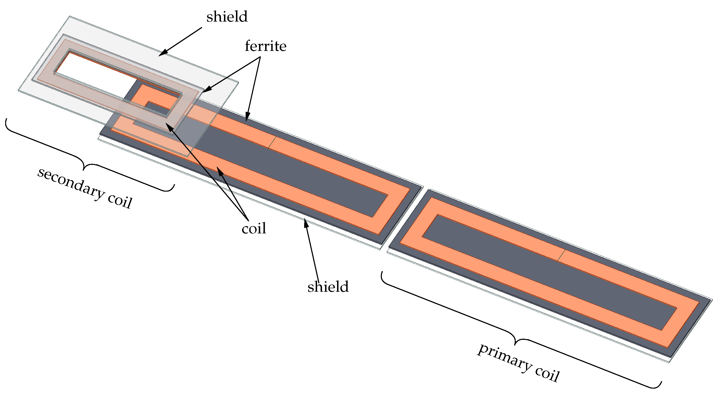
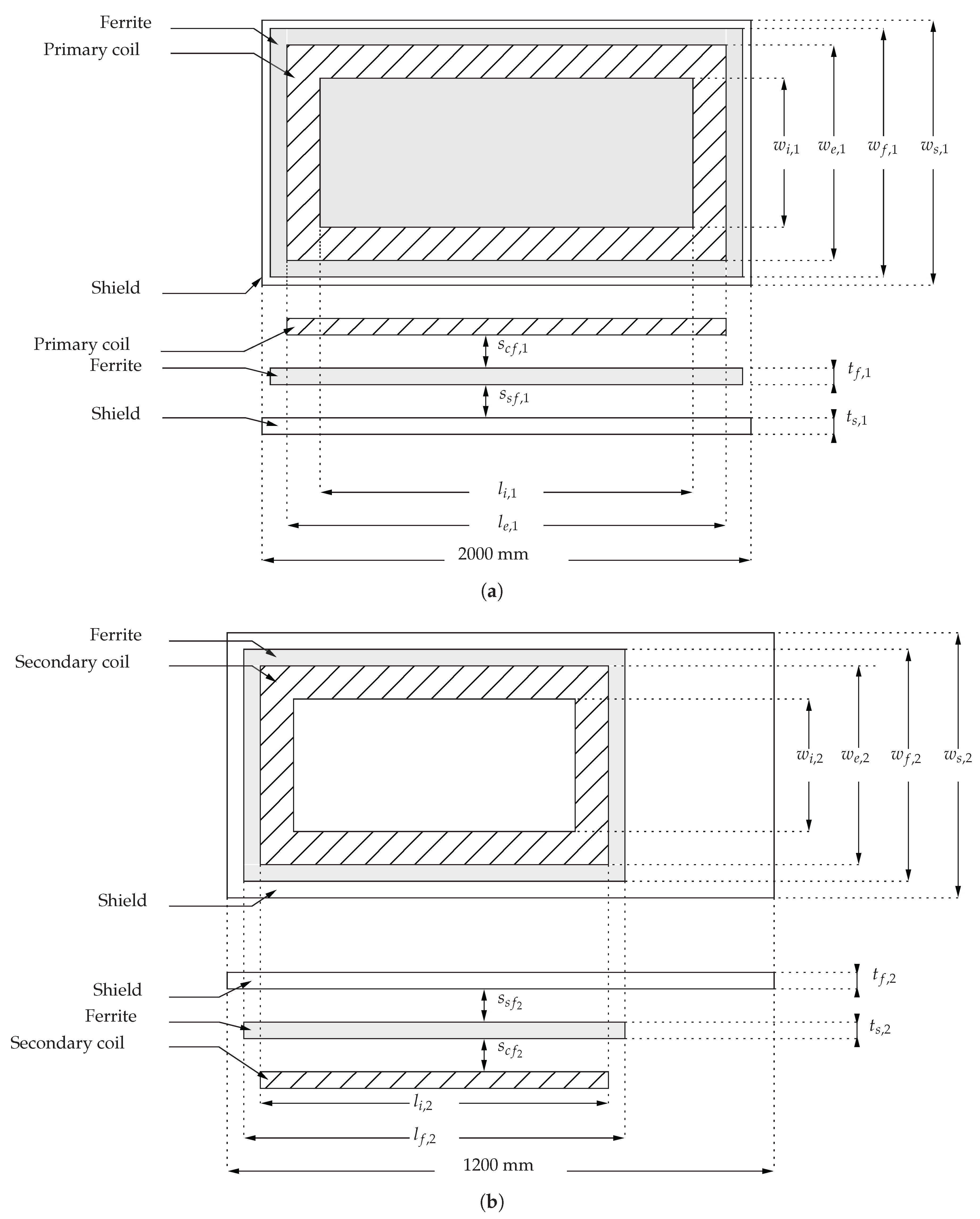
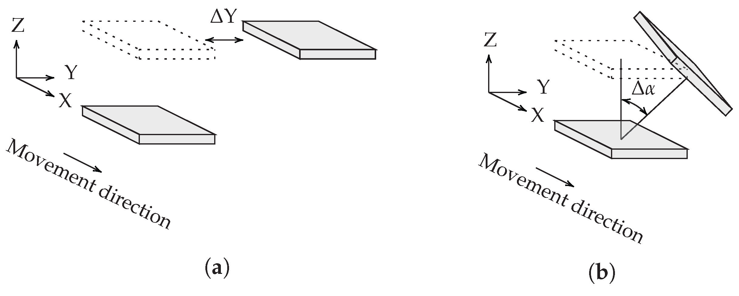
ϵ L O O 3.728 × 10 3 3.890 × 10 2 6.171 × 10 2 5.669 × 10 2
Modified ϵ L O O 4.479 × 10 3 4.256 × 10 2 6.563 × 10 2 6.233 × 10 2
Mean value0.376352.392524.247423.5579
Standard deviation0.069212.91936.64756.5193
Coefficient of variation18.390%21.659%27.415%27.674%
Table 9. Objectives and coupling-coefficient ranges for the initial design and the selected NSGA-II candidate designs.
Target R train 2 R test 2 RMSE train ( μ T ) RMSE test ( μ T )
k 11 , 2 0.99240.9467 9.531 × 10 3 2.814 × 10 2
k 12 , 2 0.99170.9488 9.940 × 10 3 2.629 × 10 2
max | B | t o p ( μ T)0.94580.6078 3.746 × 10 0 1.054 × 10 1
max | B | l e f t ( μ T)0.98330.8667 8.899 × 10 1 2.630 × 10 0
max | B | r i g h t ( μ T)0.98500.8825 9.783 × 10 1 2.607 × 10 0
Table 10. Objectives of the initial design and of the selected NSGA-II candidate geometries.
Design k 11 , 2 min k 11 , 2 max k 12 , 2 min k 12 , 2 max A 11 , 2 A 12 , 2
Initial−0.06180.3172−0.08730.30900.37890.3962
1−0.03970.3133−0.05760.32320.35300.3808
2−0.04380.3222−0.05530.29850.36590.3538
3−0.03790.3566−0.05500.39860.39450.4536
4−0.04010.3212−0.04850.32460.36130.3732
Disclaimer/Publisher’s Note: The statements, opinions and data contained in all publications are solely those of the individual author(s) and contributor(s) and not of MDPI and/or the editor(s). MDPI and/or the editor(s) disclaim responsibility for any injury to people or property resulting from any ideas, methods, instructions or products referred to in the content.