A Novel Ground Distance Protection Algorithm for Non-Uniform Power Transmission Lines

Abstract

In this paper, the performance of a conventional distance protection relay employing a single ground compensation factor (k₀) per protection zone is investigated for non-uniform transmission lines consisting of mixed overhead line and underground cable sections. In such composite lines, the use of a single k₀ value may lead to inaccurate apparent impedance calculation during phase-to-ground faults due to significant differences in zero- and positive-sequence parameters among line sections. To address this limitation, a novel ground distance protection algorithm is proposed, which applies separate ground compensation factors corresponding to individual line sections within the same distance protection zone. The proposed algorithm dynamically identifies the faulted line section based on the measured reactance and selects the appropriate compensation factor accordingly. A three-section composite transmission line model is developed in the ATP–EMTP environment, including overhead and cable segments with different electrical characteristics. Phase-to-ground faults are simulated at various locations along each line section, and the apparent impedances calculated using the proposed algorithm are quantitatively compared with those obtained from the classical ground distance protection algorithm. Simulation results demonstrate that, under resistive fault conditions (Rarc = 1 Ω), the proposed method reduces impedance magnitude estimation errors from over 23% to below 7%, while maintaining comparable or improved angle estimation accuracy across the protected zone. Although the proposed algorithm introduces an additional computational step due to the selection of appropriate ground compensation factors for individual line sections, this aspect has not been evaluated under real-time conditions and is left for future implementation-oriented studies. Overall, the proposed approach offers a practical and effective solution for improving ground distance protection performance in non-uniform transmission lines.

1. Introduction

Transmission and distribution networks in Türkiye and many other countries experiencing rapid economic growth are undergoing significant transformation. Industrial development, urban expansion, and increasing electricity demand have placed considerable pressure on existing transmission infrastructure. To address these challenges in a cost-effective manner, transmission system operators are investing not only in new transmission corridors but also in upgrading and reconfiguring existing lines. In practice, this often leads to transmission lines composed of different sections, such as overhead lines combined with underground cable segments, or sections employing different conductor types and circuit configurations. Although uniform transmission line configurations are generally preferred from a protection and operation perspective, constraints related to expropriation, urbanization, and investment costs frequently make such uniformity impractical.

Distance protection relays remain the primary protection scheme for transmission lines due to their well-established advantages, including relative insensitivity to short-circuit current magnitude, inherent backup capability, fault location functionality, load encroachment handling, and power swing detection. The operating principles, practical implementation details, and ground distance measurement concepts of distance protection relays are extensively documented in manufacturer manuals and application guides provided by major relay vendors such as Schneider Electric, Schweitzer Engineering Laboratories, Siemens, Hitachi Energy, and GE Vernova [1,2,3,4,5]. The general operating principles and practical considerations of ground distance protection have also been comprehensively reviewed in the literature [6].

Previous studies addressing the performance limitations of distance protection relays can be broadly classified into three main categories. The first category focuses on the impact of arc resistance on apparent impedance calculation, particularly for phase-to-ground faults. In such cases, unknown and time-varying fault resistance may introduce significant reach errors and compromise relay selectivity. Classical compensation approaches were proposed in early studies, while more recent works have revisited this problem using improved modeling and simulation techniques to better capture arcing behavior and impedance measurement errors [7,8,9,10]. Recent studies have also addressed fault resistance compensation in distance protection schemes, particularly for transmission lines connected to renewable energy sources such as photovoltaic plants [11].

The second category investigates the influence of mutual coupling and parallel or multi-circuit transmission lines. Zero-sequence coupling between adjacent circuits significantly affects ground distance measurements and may lead to relay misoperation if not properly compensated. Both classical and modern studies have demonstrated that mutual coupling can distort apparent impedance trajectories, particularly under resistive ground fault conditions, and various compensation and adaptive schemes have been proposed to mitigate these effects [12,13,14].

The third category, which has received comparatively limited attention, concerns distance protection applied to composite or non-uniform transmission lines consisting of different conductor types, circuit configurations, or combinations of overhead lines and underground cables. Mixed transmission lines exhibit pronounced variations in zero-sequence impedance and X₀/X₁ ratios between sections, which directly affect ground distance measurements. Several studies have addressed protection challenges in mixed or cascaded overhead–cable systems and hybrid transmission lines; however, most of these works focus on fault location accuracy or protection coordination rather than the internal behavior of ground distance algorithms themselves [15,16,17,18]. More recently, combined protection and fault location algorithms have been proposed for mixed or hybrid transmission lines; however, these methods typically rely on complex signal processing and do not explicitly address ground distance compensation within a single protection zone [19,20].

As a consequence of this limited consideration of parameter non-uniformity, distance protection relays applied to composite transmission lines may calculate inaccurate apparent impedance during phase-to-ground faults. Transmission lines composed of sections with different electrical characteristics may cause conventional distance protection algorithms to exhibit overreach or underreach behavior, potentially leading to incorrect zone operation and reduced protection selectivity.

The primary reason for these inaccuracies is that conventional ground distance protection algorithms implicitly assume that each protection zone corresponds to a uniform transmission line. Under this assumption, a single ground compensation factor is applied throughout the zone. While this simplification facilitates relay setting and implementation, it becomes problematic for non-uniform transmission lines, particularly those combining overhead and underground sections with significantly different zero-sequence characteristics.

Although existing literature has extensively addressed arc resistance effects, mutual coupling, and parallel-line configurations, the specific impact of electrical parameter non-uniformity within a single protection zone remains insufficiently investigated. In particular, most existing approaches continue to rely on a single ground compensation factor and implicitly assume uniform line parameters within each protection zone, even for composite overhead–cable or hybrid transmission lines. A systematic comparison of representative studies in the literature, summarized in

Table 1. Comparison of existing ground distance protection approaches and the proposed method.

Study/Approach	Line Type Considered	Ground Compensation Strategy	Single Protection Zone Assumption	Section Identification	Main Limitation
Smith et al. [6]	Uniform overhead lines	Single fixed k0 per zone	Yes	No	Assumes uniform line parameters
Bharti et al. [7]	Parallel overhead lines	Fault resistance compensation	Yes	No	Focused on mutual coupling, not line non-uniformity
Blumschein & Dzienis [9]	Overhead lines	Arc resistance compensation	Yes	No	Does not address composite line sections
Tziouvaras & Needs [15]	Mixed OHL–cable lines	Conventional k0	Yes	No	Protection accuracy degradation not quantitatively addressed
Zahran et al. [16]	Cascaded OHL–cable	Modified impedance calculation	Yes	No	Static compensation approach
Aminirad & Shahrtash [19]	Hybrid lines	Combined protection & fault location	Yes	No	Increased algorithmic complexity
Proposed Method (This Paper)	Non-uniform composite lines	Section-dependent adaptive k0	Yes	Yes	—

, reveals that while various protection enhancements have been proposed, none explicitly integrate dynamic section identification and section-dependent ground compensation within a single distance protection zone. Consequently, the implications of employing a single ground compensation factor for composite transmission lines—especially in terms of reach accuracy and impedance trajectory behavior under ground faults—have not been comprehensively analyzed.

Motivated by this research gap, this study evaluates the performance of a conventional phase-to-ground distance protection algorithm employing a single ground compensation factor and compares it with a newly proposed approach designed for non-uniform transmission lines. The proposed method dynamically identifies the faulted line section within a single protection zone based on the measured reactance and applies a section-specific ground compensation factor corresponding to the identified line segment.

Unlike existing approaches that treat section-dependent compensation as a static setting or rely on averaged parameters, the proposed algorithm integrates section-dependent ground compensation directly into the distance protection algorithm itself. This enables adaptive operation within a single protection zone without increasing setting complexity. The effectiveness of the proposed approach is validated through ATP–EMTP simulations conducted on a three-section composite transmission line consisting of overhead and underground segments, and its performance is quantitatively compared with that of the conventional ground distance protection algorithm.

The main contributions of this paper can be summarized as follows:

• A novel ground distance protection algorithm is proposed for non-uniform transmission lines, which dynamically identifies the faulted line section within a single protection zone and applies the corresponding ground compensation factor.
• The limitations of conventional distance protection relays employing a single ground compensation factor per zone are quantitatively demonstrated for composite overhead–cable transmission lines using ATP–EMTP simulations.
• Simulation results show that the proposed algorithm significantly reduces apparent impedance estimation errors, particularly in the middle of the protection zone, thereby mitigating overreach and underreach problems under resistive fault conditions.
• Unlike conventional methods based on a single averaged compensation factor, the proposed approach employs section-specific ground compensation factors and integrates faulted section identification into the distance measurement process, providing improved accuracy for non-uniform transmission lines with a practical and implementable protection scheme.

The remainder of this paper is organized as follows. Section 2 presents the conventional phase-to-ground distance measurement principle and introduces the proposed section-based ground distance protection algorithm. Section 3 describes the ATP–EMTP simulation model and fault scenarios applied to a non-uniform transmission line. Section 4 provides a comparative performance analysis between the classical and proposed algorithms, and Section 5 concludes the paper.

2. Proposed Ground Distance Algorithm

This section introduces the proposed ground distance protection algorithm. As a preliminary step, the conventional phase-to-ground distance measurement principle is briefly reviewed to highlight the implicit assumptions associated with a single compensation factor. These assumptions form the motivation for the proposed algorithm developed in the subsequent subsection.

2.1. Conventional Phase-to-Ground Distance Measurement

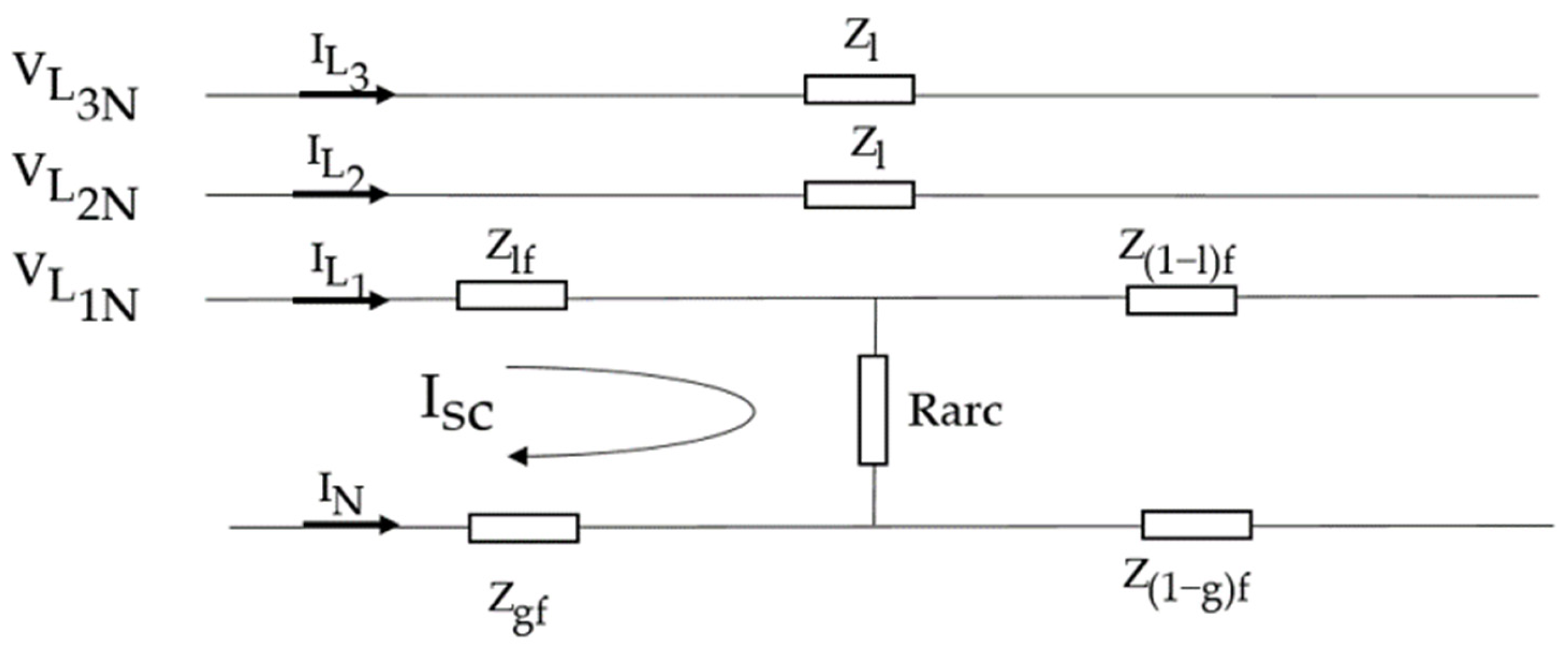
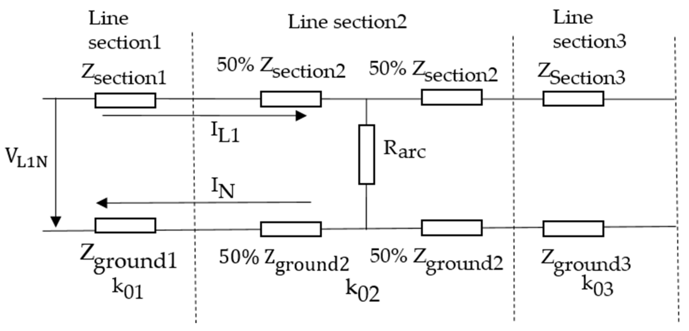
For an L1 phase-to-ground fault, as shown in Figure 1, the distance protection relay initially detects the faulty phase and subsequently computes the apparent impedance. This calculation is performed using Equation (4), which is obtained by transforming Equation (1). In Equation (4), the ground impedance term ${(\mathrm{Z}}_{\mathrm{g}})$ is eliminated by incorporating the zero-sequence compensation factor ${\mathrm{k}}_0$.

$${\mathrm{V}}_{\mathrm{L}1\mathrm{N}}={ \mathrm{I}}_{\mathrm{L}1} \times {\mathrm{Z}}_{\mathrm{L}}-{\mathrm{I}}_{\mathrm{N}} \times {\mathrm{Z}}_{\mathrm{g}}$$

(1)

$${\mathrm{Z}}_{\mathrm{g}}={\displaystyle \frac{{\mathrm{Z}}^0-{ \mathrm{Z}}^{+}}{3}}$$

(2)

The parameter ${\mathrm{k}}_0$ is referred to as the standard ground compensation factor and is defined as the ratio of the ground impedance to the line impedance as shown in Equation (3).

$${\mathrm{k}}_0={\displaystyle \frac{{\mathrm{Z}}_{\mathrm{g}}}{{\mathrm{Z}}_{\mathrm{L}}}}={\displaystyle \frac{{\mathrm{Z}}^0-{\mathrm{Z}}^{+}}{3{\mathrm{Z}}^{+}}}$$

(3)

$${ \mathrm{V}}_{\mathrm{L}1\mathrm{N}}={ \mathrm{I}}_{\mathrm{L}1} \times { \mathrm{Z}}_{\mathrm{L} }-{\mathrm{I}}_{\mathrm{N}} \times {\mathrm{k}}_0 \times { \mathrm{Z}}_{\mathrm{L}}$$

(4)

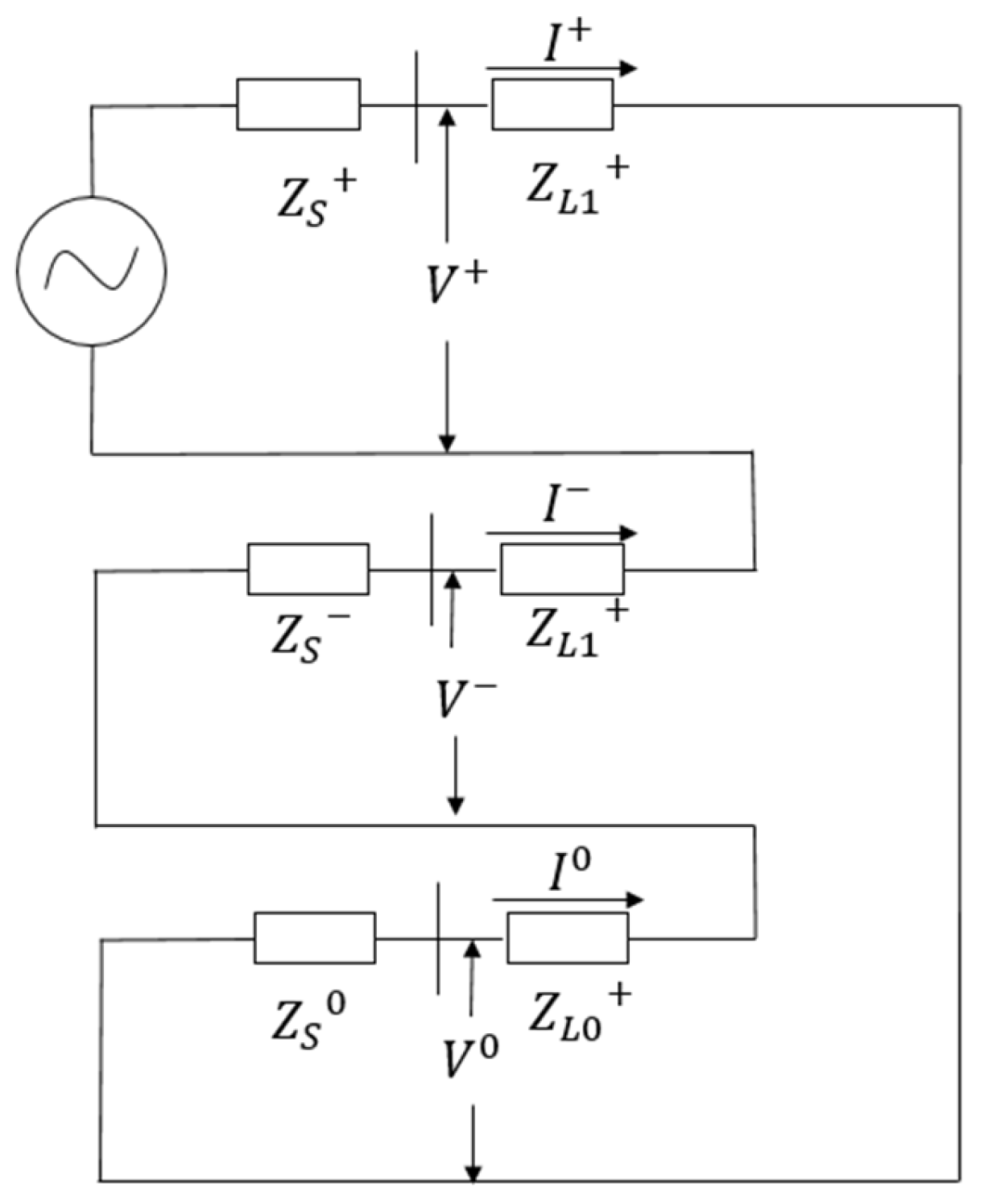
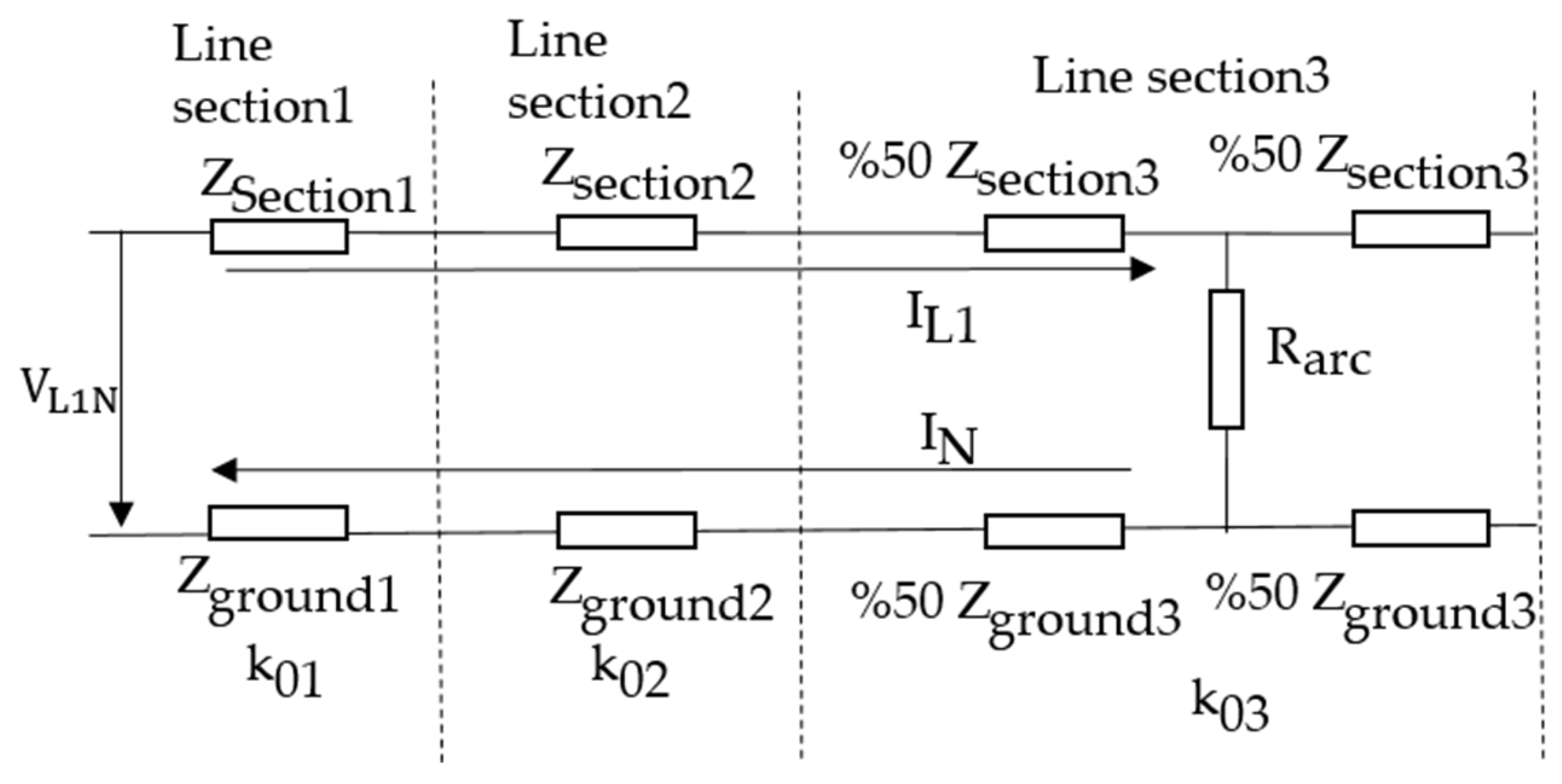
Using the method of symmetrical components, as illustrated in Figure 2, phase-to-earth faults are analyzed by connecting the positive-, negative-, and zero-sequence networks in series.

$${\mathrm{V}}_{\mathrm{L}1}={\mathrm{V}}^{+}+{ \mathrm{V}}^{-}+{ \mathrm{V}}^0$$

(5)

$${\mathrm{I}}_{\mathrm{L}1}={\mathrm{I}}^{+}+{\mathrm{I}}^{-}+{\mathrm{I}}^0$$

(6)

$${\mathrm{I}}_{\mathrm{N}}=-3{\mathrm{I}}^0$$

(7)

In transmission lines, the positive-sequence impedance is typically equal to the negative-sequence impedance.

$${\mathrm{Z}}^{+}={\mathrm{Z}}^{-}={ \mathrm{Z}}_{\mathrm{L}}$$

(8)

$${\mathrm{V}}_{\mathrm{L}1\mathrm{N}}={ \mathrm{Z}}^{+} \times {\mathrm{I}}^{+}+{\mathrm{Z}}^{-} \times {\mathrm{I}}^{-}+{ \mathrm{Z}}^0 \times {\mathrm{I}}^0$$

(9)

$${\mathrm{V}}_{\mathrm{L}1\mathrm{N}}={ \mathrm{Z}}^{+} \times \left({\mathrm{I}}^{+}+{\mathrm{I}}^{-}\right)+{\mathrm{Z}}^0 \times {\mathrm{I}}^0$$

(10)

By substituting Equations (5)–(8) into Equation (10), Equation (16) is obtained. Equation (16) expresses the relationship between the relay-calculated impedance, the voltages and currents measured by the relay, and the ground compensation factor.

$${\mathrm{V}}_{\mathrm{L}1\mathrm{N}}={\mathrm{Z}}^{+} \times \left({\mathrm{I}}_{\mathrm{L}1}-{\mathrm{I}}^0\right)+{\mathrm{Z}}^0 \times { \mathrm{I}}^0$$

(11)

$${\mathrm{V}}_{\mathrm{L}1\mathrm{N}}={ \mathrm{Z}}^{+} \times {\mathrm{I}}_{\mathrm{L}1}-{{\mathrm{Z}}^{+} \times \mathrm{I}}^0+{\mathrm{Z}}^0 \times {\mathrm{I}}^0$$

(12)

$${\mathrm{V}}_{\mathrm{L}1\mathrm{N}}={\mathrm{Z}}^{+} \times {\mathrm{I}}_{\mathrm{L}1}+{ (\mathrm{Z}}^0-{\mathrm{Z}}^{+}) \times {\mathrm{I}}^0$$

(13)

$${\mathrm{V}}_{\mathrm{L}1\mathrm{N}}={\mathrm{Z}}^{+} \times {\mathrm{I}}_{\mathrm{L}1}+{(\mathrm{Z}}^0-{\mathrm{Z}}^{+}) \times {\displaystyle \frac{-{\mathrm{I}}_{\mathrm{N}}}{3}}$$

(14)

$${\mathrm{V}}_{\mathrm{L}1\mathrm{N}}={ \mathrm{Z}}^{+}\left({\mathrm{I}}_{\mathrm{L}1}+{\displaystyle \frac{{(\mathrm{Z}}^0-{\mathrm{Z}}^{+})}{{\mathrm{Z}}^{+}}} \times {\displaystyle \frac{-{\mathrm{I}}_{\mathrm{N}}}{3}}\right)$$

(15)

$${\mathrm{V}}_{\mathrm{L}1\mathrm{N}}={\mathrm{Z}}_{\mathrm{L}}\left({\mathrm{I}}_{\mathrm{L}1}-{\mathrm{k}}_0 \times {\mathrm{I}}_{\mathrm{N}}\right)$$

(16)

For uniform transmission lines, the ground compensation factor can be readily calculated using (3). However, for non-uniform transmission lines composed of sections with different electrical characteristics, protection engineers commonly adopt one of the following two approaches to determine a single ground compensation factor

In the first approach, referred to as the average ground compensation factor method, the ground compensation factors calculated individually for each line section are arithmetically averaged. Accordingly, the individual ${\mathrm{k}}_{0,\mathrm{n}}$ values corresponding to each section are summed and divided by the total number of line sections. This method is frequently applied in practice due to its simplicity, particularly when a single compensation factor is required for the entire protection zone. The corresponding formulation is given below.

$${\mathrm{k}}_0={\displaystyle \frac{{\mathrm{k}}_{01}+{\mathrm{k}}_{02 }+{\mathrm{k}}_{03} +\dots + {\mathrm{k}}_{0\mathrm{n}}}{\mathrm{n}}}$$

(17)

$${\mathrm{k}}_0={\displaystyle \frac{\sum _1^{\mathrm{n}}{\mathrm{k}}_{0\mathrm{n}}}{\mathrm{n}}}$$

(18)

In the second approach, the ground compensation factor is derived directly from the total zero-sequence and positive-sequence impedances of the composite transmission line. In this case, the overall line impedance is obtained by summing the sequence impedances of all individual sections, and the ground compensation factor is then calculated using these equivalent total impedances. This method reflects the aggregated electrical behavior of the non-uniform line and is expressed by the following equations.

$${\mathrm{Z}}^{+}= ( {\mathrm{r}}_1^{+}+{\mathrm{r}}_2^{+}+{ \mathrm{r}}_3^{+} +\dots )+{ \mathrm{i}(\mathrm{x}}_1^{+}+{\mathrm{x}}_2^{+}+{ \mathrm{x}}_3^{+} +\dots )$$

(19)

$${\mathrm{Z}}^0={ (\mathrm{r}}_1^0+{\mathrm{r}}_2^0+{ \mathrm{r}}_3^0 +\dots )+{\mathrm{i}(\mathrm{x}}_1^0+{\mathrm{x}}_2^0+{\mathrm{x}}_3^0 +\dots )$$

(20)

$${\mathrm{k}}_0={\displaystyle \frac{{\left[{(\mathrm{r}}_{1 }^0+{\mathrm{r}}_2^0+{\mathrm{r}}_3^0+\dots \right)-(\mathrm{r}}_1^{+}+{\mathrm{r}}_2^{+}+{\mathrm{r}}_3^{+}+\dots \left)\right]+\mathrm{i}[{(\mathrm{x}}_1^0+{\mathrm{x}}_2^0+{\mathrm{x}}_3^0+\dots ) -{(\mathrm{x}}_1^{+}+{\mathrm{x}}_2^{+}+{ \mathrm{x}}_3^{+}+\dots \left)\right]}{3[{(\mathrm{r}}_1^{+}+{\mathrm{r}}_2^{+}+{\mathrm{r}}_3^{+} +\dots )+{\mathrm{i}(\mathrm{x}}_1^{+}+{ \mathrm{x}}_2^{+}+{\mathrm{x}}_3^{+}+\dots \left)\right] }}$$

(21)

$${\mathrm{k}}_0={\displaystyle \frac{\sum _1^{\mathrm{n}}{\left[\right(\mathrm{r}}_{\mathrm{n}}^0-{\mathrm{r}}_{\mathrm{n}}^{+})+\mathrm{i}\sum _1^{\mathrm{n}}{(\mathrm{x}}_{\mathrm{n}}^0-{\mathrm{x}}_{\mathrm{n}}^{+}\left)\right]}{3\sum _1^{\mathrm{n}}{(\mathrm{r}}_{\mathrm{n}}^{+}-{\mathrm{x}}_{\mathrm{n}}^{+})}}$$

(22)

2.2. Proposed Section-Based Ground Distance Algorithm

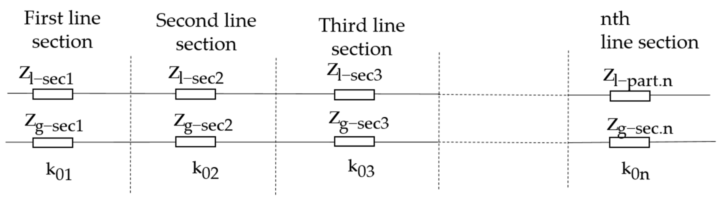
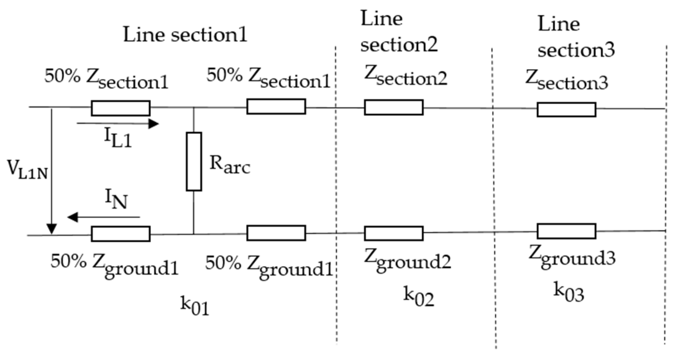
Transmission lines may be represented as multiple line segments with distinct electrical characteristics. The proposed ground distance protection algorithm utilizes individual ground and coupling compensation factors for each segment in non-uniform transmission lines. Following fault detection, the relay determines the fault cycle and evaluates the phase-to-ground loop. The faulted line segment is identified based on the reactance measured during the fault, which is assumed to be insensitive to fault arc resistance. Subsequently, the appropriate compensation factors are selected, and the impedance calculation proceeds according to the proposed equations until the relay issues a trip command. The N-section transmission line representation adopted to model the non-uniform line structure is illustrated in Figure 3.

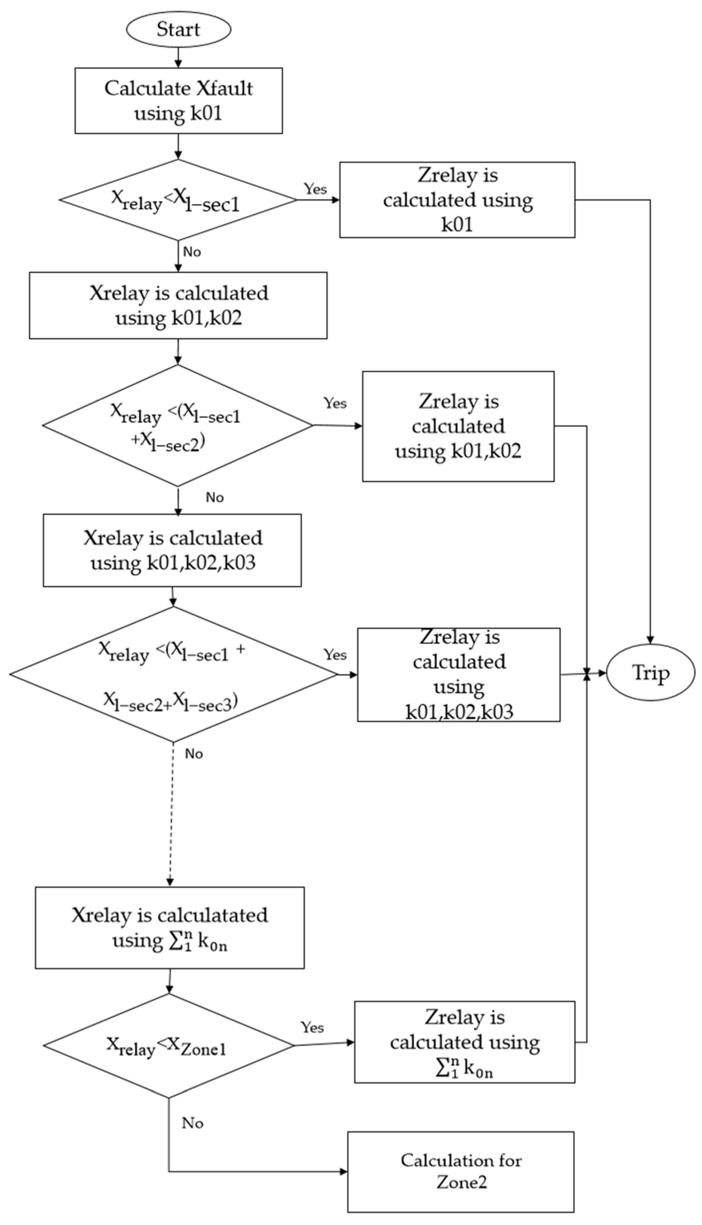
Based on the proposed algorithm, the relay selects the appropriate phase-to-ground loop and computes the impedance using Equation (23).

$${\mathrm{Z}}_{\mathrm{Relay}}={\displaystyle \frac{{\mathrm{V}}_{\mathrm{L}1\mathrm{N}}}{{\mathrm{I}}_{\mathrm{L}1}-{\mathrm{I}}_{\mathrm{N}} \times {\mathrm{k}}_{01}}}$$

(23)

$${\mathrm{Z}}_{\mathrm{R}\mathrm{e}\mathrm{l}\mathrm{a}\mathrm{y}}={\mathrm{R}}_{\mathrm{R}\mathrm{e}\mathrm{l}\mathrm{a}\mathrm{y}}+\mathrm{j}{\mathrm{X}}_{\mathrm{R}\mathrm{e}\mathrm{l}\mathrm{a}\mathrm{y}}$$

(24)

If the condition ${\mathrm{X}}_{\mathrm{relay}} <{ \mathrm{X}}_{\mathrm{l}-\sec 1}$ is satisfied, the impedance is computed using Equation (23) until the relay operates.

If ${\mathrm{X}}_{\mathrm{relay}} >{ \mathrm{X}}_{\mathrm{l}-\sec 1}$, the algorithm determines that the fault is not within the first line section, and ${\mathrm{X}}_{\mathrm{r}\mathrm{e}\mathrm{l}\mathrm{a}\mathrm{y}}$ is recalculated according to Equation (25).

$${\mathrm{Z}}_{\mathrm{Relay}}={\displaystyle \frac{{\mathrm{V}}_{\mathrm{L}1\mathrm{N}}}{{\mathrm{I}}_{\mathrm{L}1}-{\mathrm{I}}_{\mathrm{N}} \times {(\mathrm{k}}_{01}+{\mathrm{k}}_{02})}}$$

(25)

If ${\mathrm{X}}_{\mathrm{relay}} <{ \mathrm{X}}_{\mathrm{l}-\sec 2}$, the fault is determined to be located in the second line section, and the impedance is calculated using Equation (25) until the relay issues a trip decision. If ${\mathrm{X}}_{\mathrm{relay}} > {\mathrm{X}}_{\mathrm{l}-\sec 2}$ is calculated using Equation (26).

$${\mathrm{Z}}_{\mathrm{Relay}}={\displaystyle \frac{{\mathrm{V}}_{\mathrm{L}1\mathrm{N}}}{{\mathrm{I}}_{\mathrm{L}1}-{ \mathrm{I}}_{\mathrm{N}} \times {(\mathrm{k}}_{01}+{ \mathrm{k}}_{02}+{ \mathrm{k}}_{03})}}$$

(26)

The above calculations are iteratively applied to all line sections. For a transmission line composed of n sections, the impedance corresponding to the nth section is computed using Equation (27). The overall computational procedure of the proposed algorithm is summarized in the flowchart shown in Figure 4.

$${\mathrm{Z}}_{\mathrm{Relay}}={\displaystyle \frac{{\mathrm{V}}_{\mathrm{L}1\mathrm{N}}}{{\mathrm{I}}_{\mathrm{A}}-{\mathrm{I}}_{\mathrm{N}} \times \sum _1^{\mathrm{n}}{\mathrm{k}}_{0\mathrm{n}} }}$$

(27)

3. Simulation Model of a Non-Uniform Three-Section Transmission Line

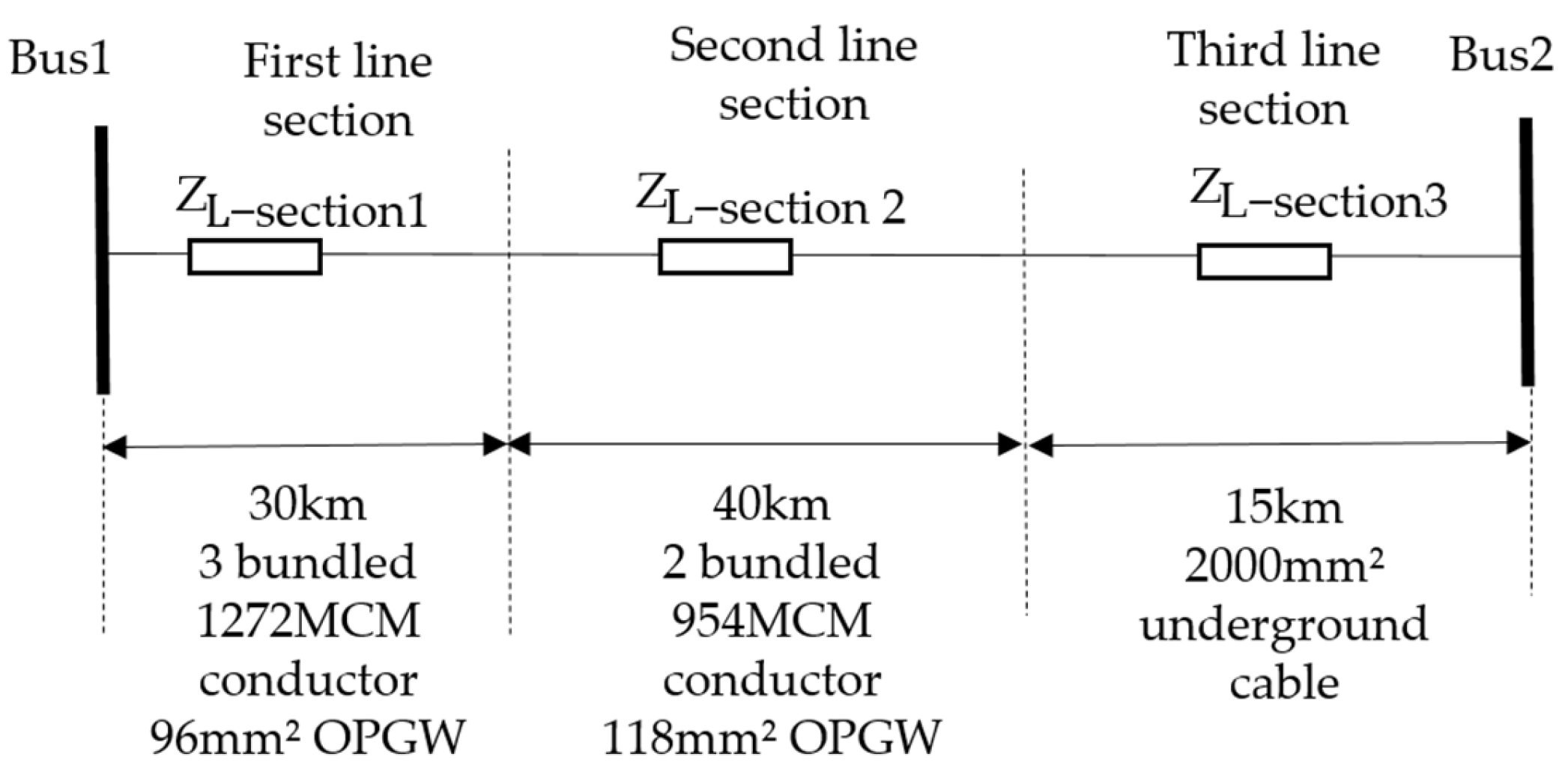
A three-section transmission line was modeled in the ATP–EMTP environment, as illustrated in Figure 5. The first two sections consist of overhead lines, whereas the third section is an underground cable. Figure 5 illustrates the physical configuration and lengths of the three transmission line sections.

The first transmission line section is modeled as a three-bundle 1272 MCM overhead line with a 96 mm² OPGW ground wire, while the second section consists of a two-bundle 954 MCM overhead line equipped with a 118 mm² OPGW. The third section represents a 2000 mm² underground cable.

The non-uniform transmission line is modeled using a π-equivalent representation for each line section in the ATP–EMTP environment. The sending-end and receiving-end buses are represented by their Thevenin equivalents to realistically model the source and system strength. At Bus 1, the positive-sequence Thevenin impedance is assumed as 1.1393 + i20.64026 Ω, while the zero-sequence Thevenin impedance is 15.2765 + 20.74186 Ω. Similarly, at Bus 2, the positive-sequence Thevenin impedance is modeled as 1.1422 + j21.05 Ω, and the corresponding zero-sequence Thevenin impedance is 15.2794 + j21.15027. These values are selected to represent a realistic transmission system environment and to ensure that the influence of source impedance on ground distance measurements is properly captured in the simulations.

All simulations are performed in the ATP–EMTP environment using a fundamental system frequency of 50 Hz. Voltage and current signals are measured at the relay location at Bus 1 and processed using fundamental frequency phasor quantities. The apparent impedance calculations are based on steady-state phasor values obtained after fault inception. A fixed simulation time step is employed to ensure numerical stability, and no additional signal filtering is applied in order to clearly observe the inherent behavior of the distance protection algorithms under ideal measurement conditions. The simulation time step is set to Δt = 1 μs to accurately capture transient fault behavior while maintaining numerical stability.

Table 2. Kilometer-based electrical parameters of the three-section transmission line.

	Line Section 1			Line Section 2			Line Section 3
	R (Ω/km)	L (mH/km)	C (µF/km)	R (Ω/km)	L (mH/km)	C (µF/km)	R (Ω/km)	L (mH/km)	C (µF/km)
${\mathrm{Z}}^{+}$	0.0161	0.853	0.0138	0.0315	1.016	0.01156	0.0137	0.638	0.1443
${\mathrm{Z}}^0$	0.2565	2.943	0.0087	0.2771	2.857	0.0082	0.0755	0.2174	0.1443

presents the parameters of the transmission line sections considered in the simulation. The electrical characteristics of the transmission lines were obtained from the Load Dispatch Information System (YTBS) of the Turkish Electricity Transmission Corporation (TEİAŞ).

The per-kilometer positive- and zero-sequence impedance parameters listed in Table 2 are scaled by the physical lengths of the individual line sections to obtain the total sequence impedances. These calculated impedances for each section, as well as the overall line impedance, are presented in

Table 3. Electrical characteristics of the three-section transmission line.

	Line Section 1 (30 km)			Line Section 2 (40 km)			Line Section 3 (15 km)
	R (Ω)	L (mH)	C (µF)	R (Ω)	L (mH)	C (µF)	R (Ω)	L (mH)	C (µF)
${\mathrm{Z}}^{+}$	0.485	25.59	0.414	1.26	40.64	0.4624	0.2055	9.57	2.1645
${\mathrm{Z}}^0$	7.695	88.29	0.261	11.084	114.28	0.328	1.1325	3.261	2.1645

.

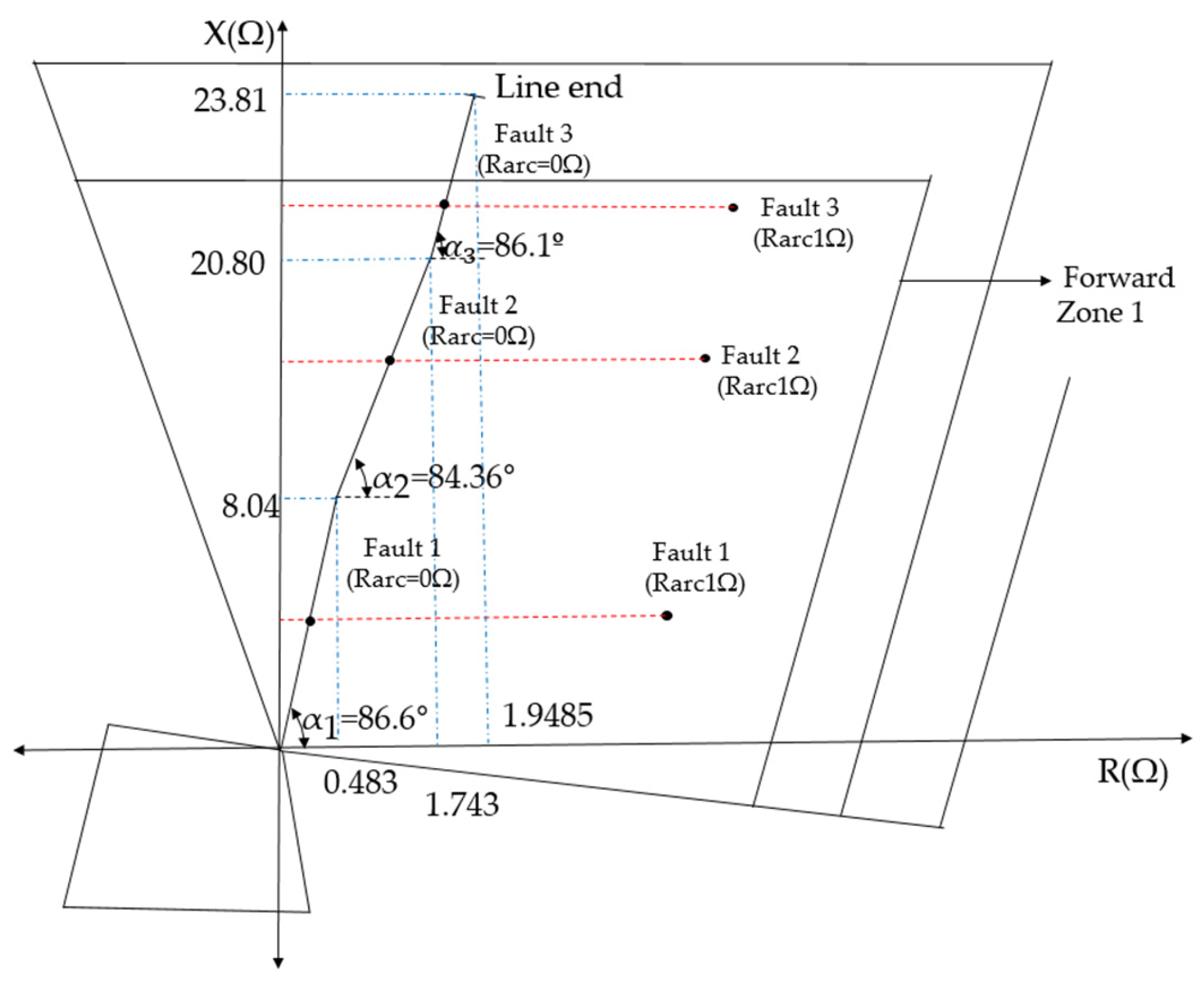
Based on the data provided in Table 3, the line impedances are calculated and reported for the first, second, and third line sections, followed by the total impedance of the transmission line. The corresponding impedance representation in the R–X plane, including section boundaries and fault locations, is illustrated in Figure 6.

$${\mathrm{Z}}_{\text{sec1}}=0.485+\mathrm{i}8.04 \mathsf{\Omega }$$

$${\mathrm{Z}}_{\text{sec2}}= 1.26 +\mathrm{i}12.75 \mathsf{\Omega }$$

$${\mathrm{Z}}_{\text{sec3}}=0.2055+\mathrm{i}3.0105 \mathsf{\Omega }$$

$${\mathrm{Z}}_{\mathrm{total}}=1.9485+\mathrm{i}23.81 \mathsf{\Omega }$$

The simulated system operates at a bus phase to phase voltage of 420 kV. To evaluate and compare the performance of the conventional and proposed distance protection algorithms under non-uniform line conditions, single phase-to-ground (L1–G) faults are systematically applied at the midpoint of each transmission line section. A total of six fault scenarios are analyzed. In the first three scenarios, the arc resistance is set to zero in order to establish a baseline condition, whereas an arc resistance of 1 Ω is introduced in the remaining scenarios to assess the impact of fault resistance. All faults are initiated at 100 ms.

Table 4. Impedances from busbar to fault location *.

	Z (Ω) **
First Fault	4.03$/86.56°$
Second Fault	14.47$/85.59°$
Third Fault	22.39$/85.27°$

* Not including fault resistance. ** The slash with underline notation is used to represent the phase angle of phasor quantities.

lists the apparent impedances between the sending-end busbar and the fault locations for each scenario, which serve as reference values for evaluating the impedance estimation accuracy of the distance protection algorithms.

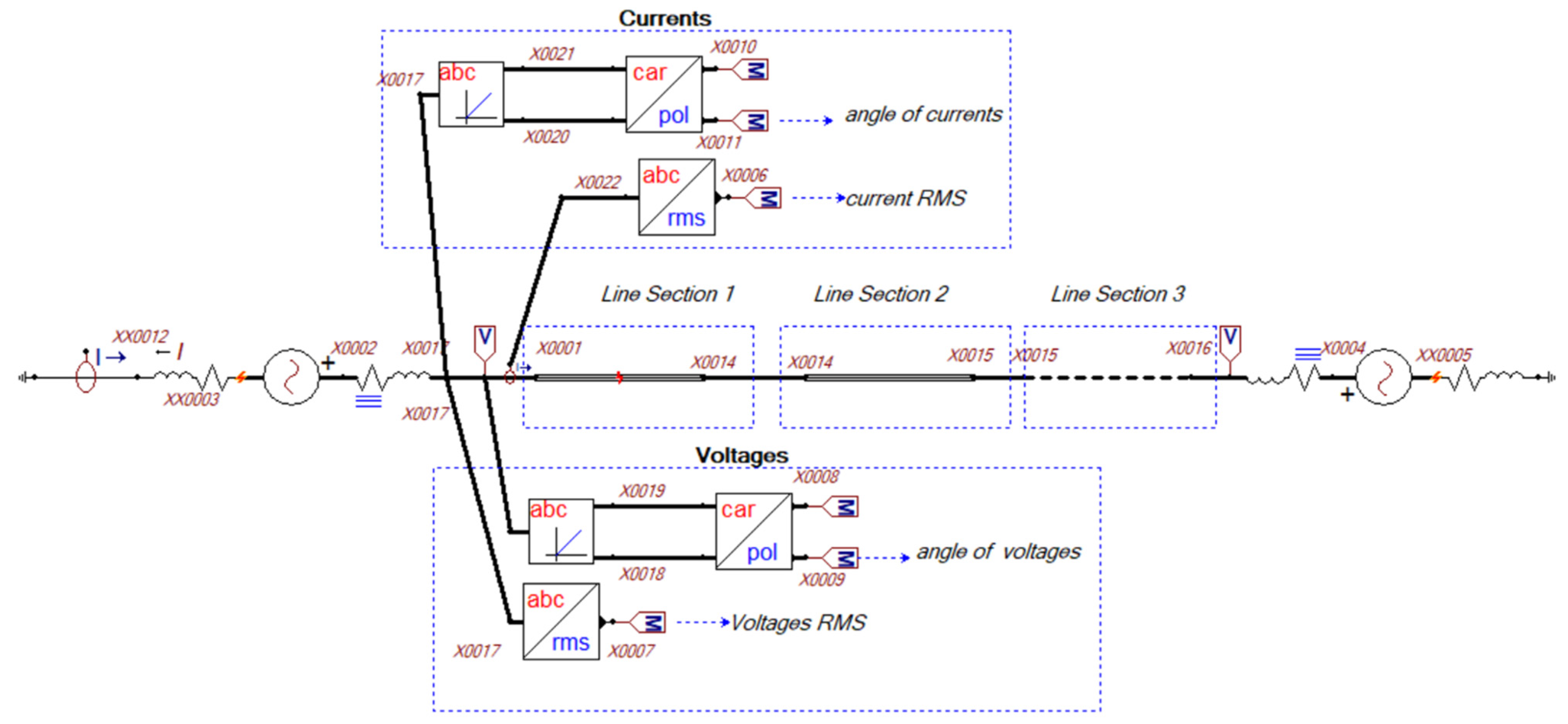
To evaluate the proposed and classical distance protection algorithms under realistic conditions, an ATP–EMTP simulation model was developed using the transmission line parameters listed in Table 3, as shown in Figure 7.

3.1. Phase–Ground Fault in the First Section

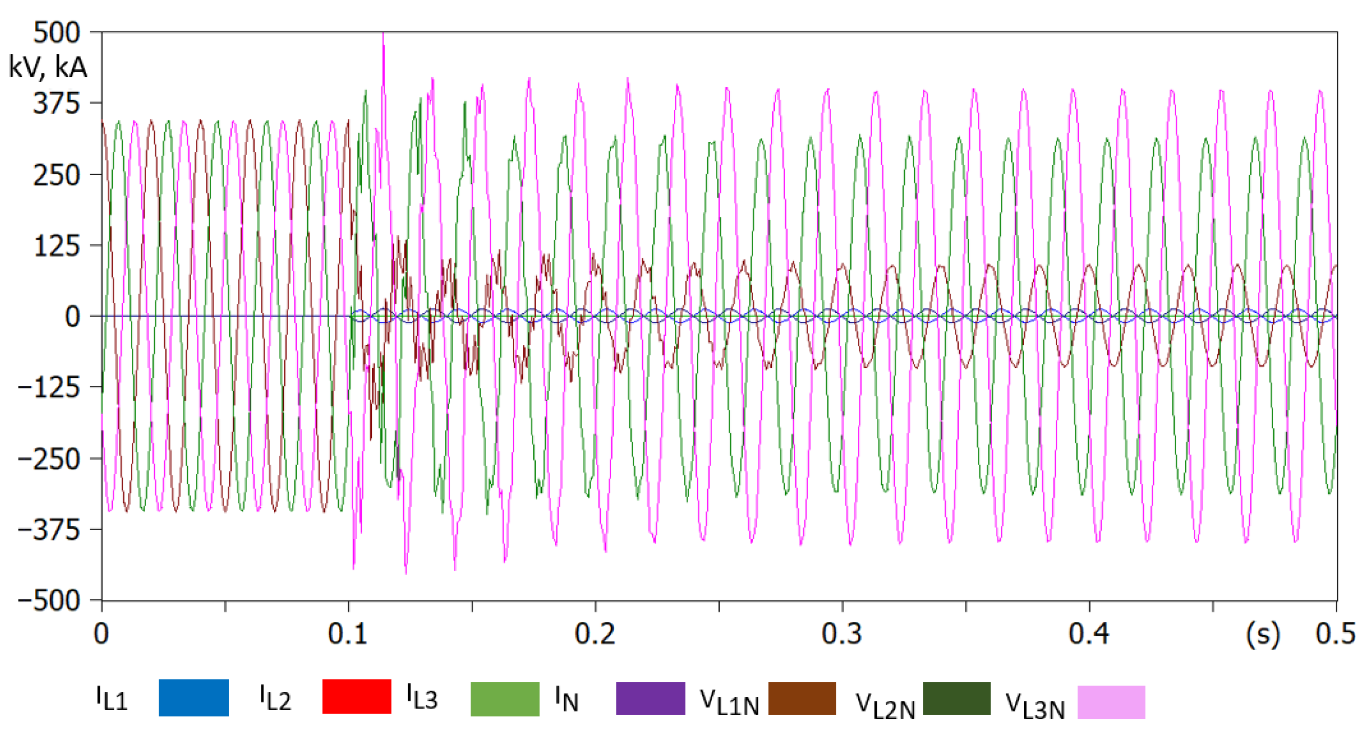
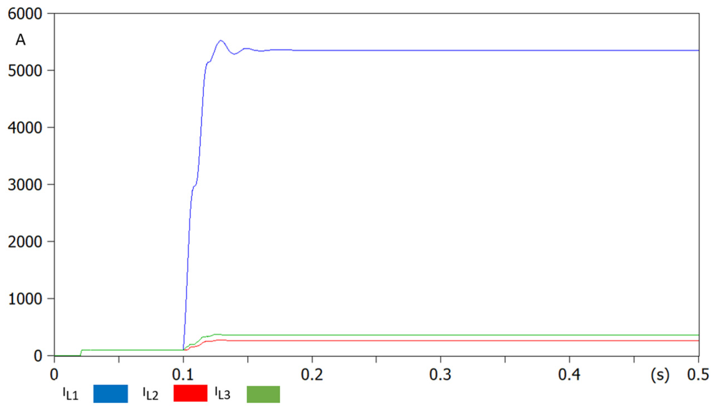
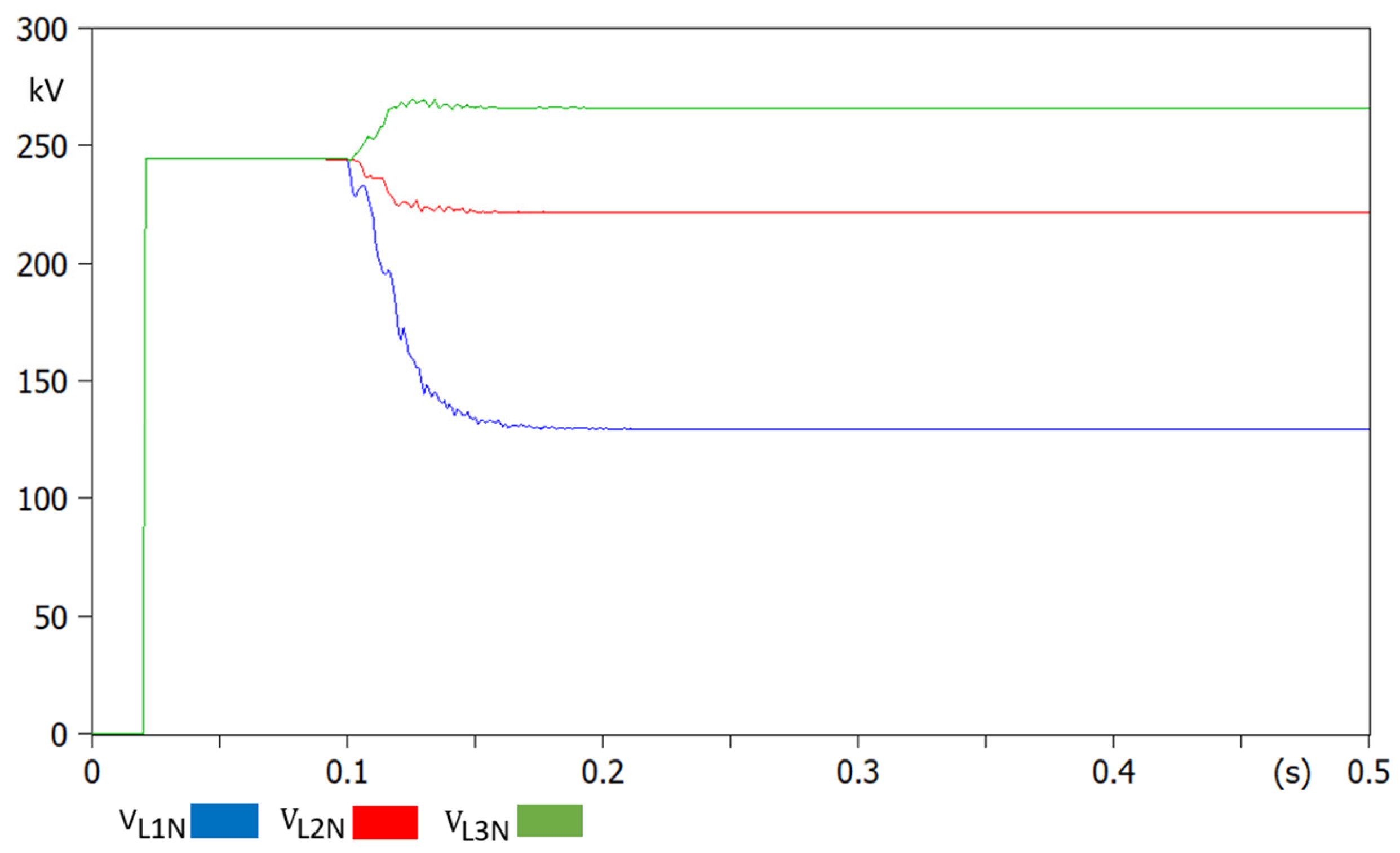
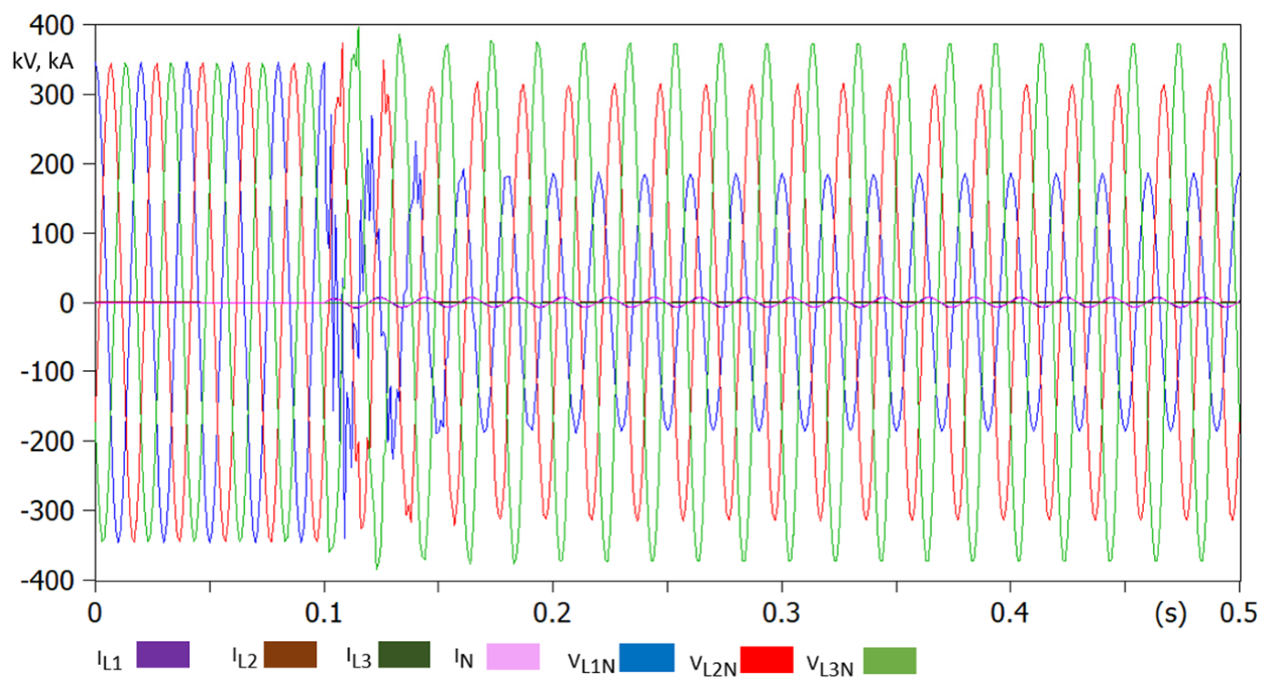
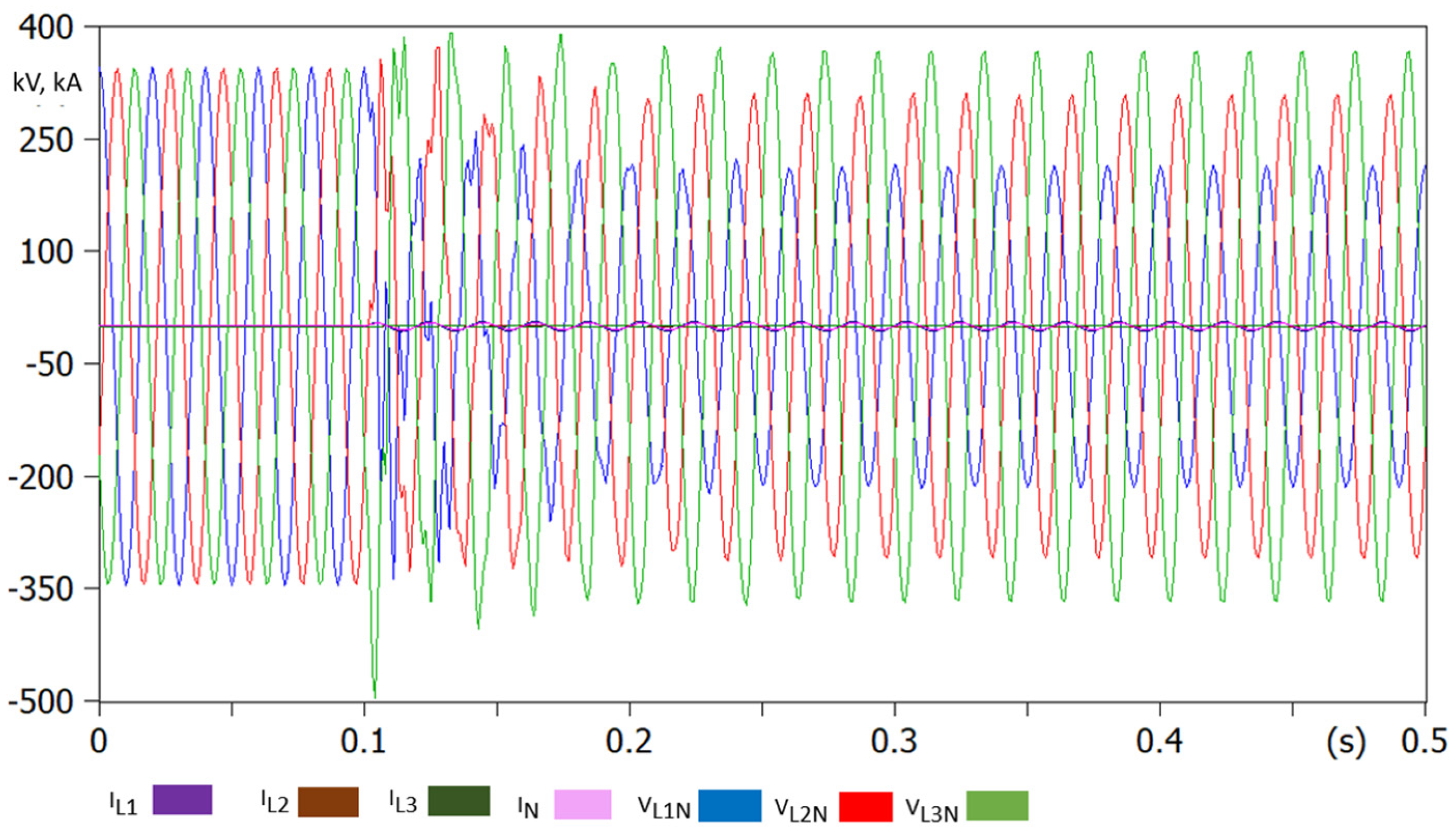
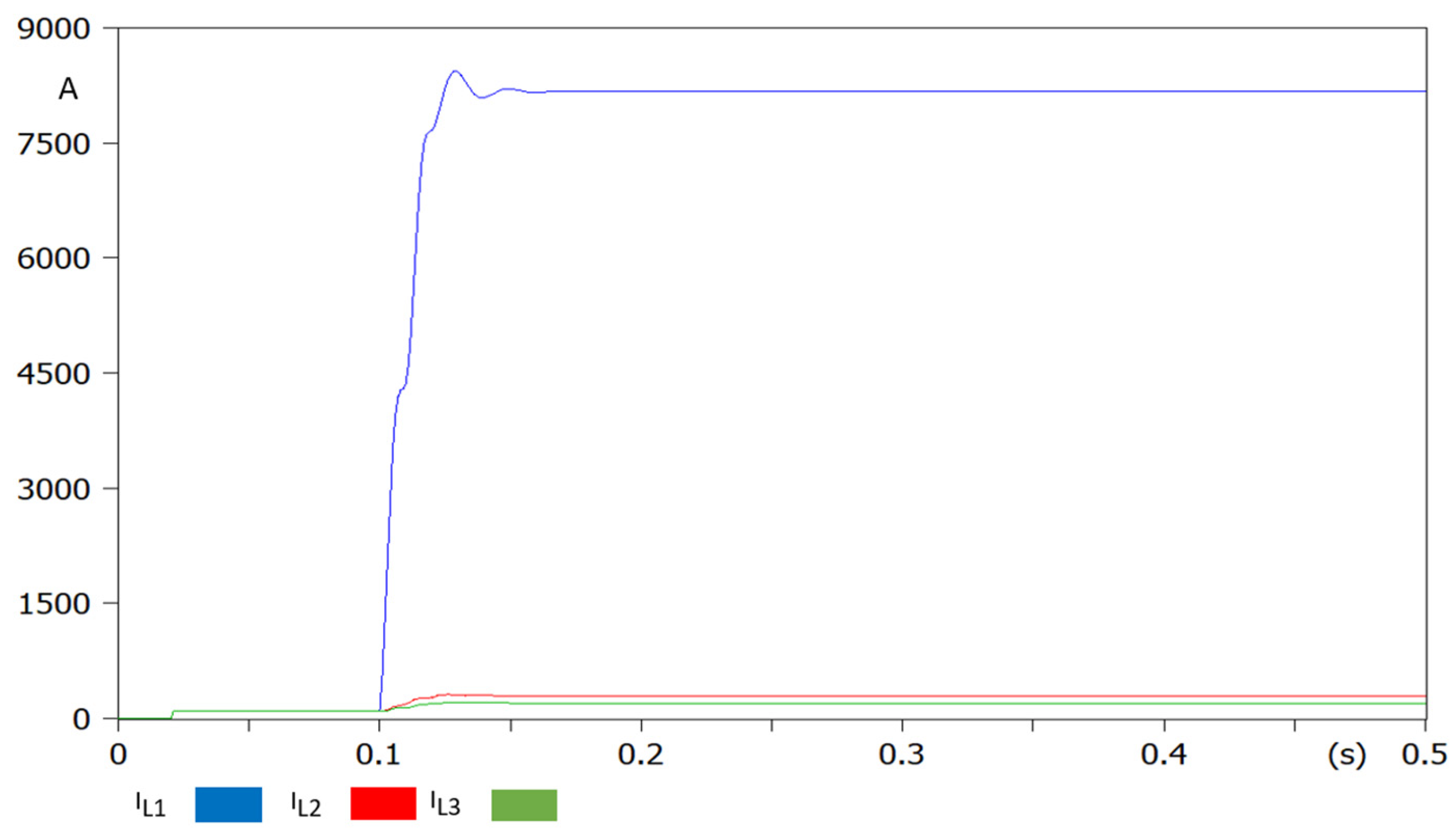
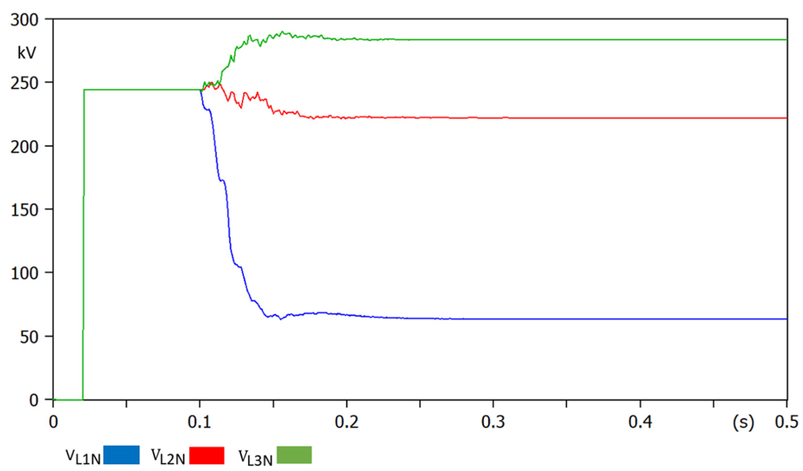
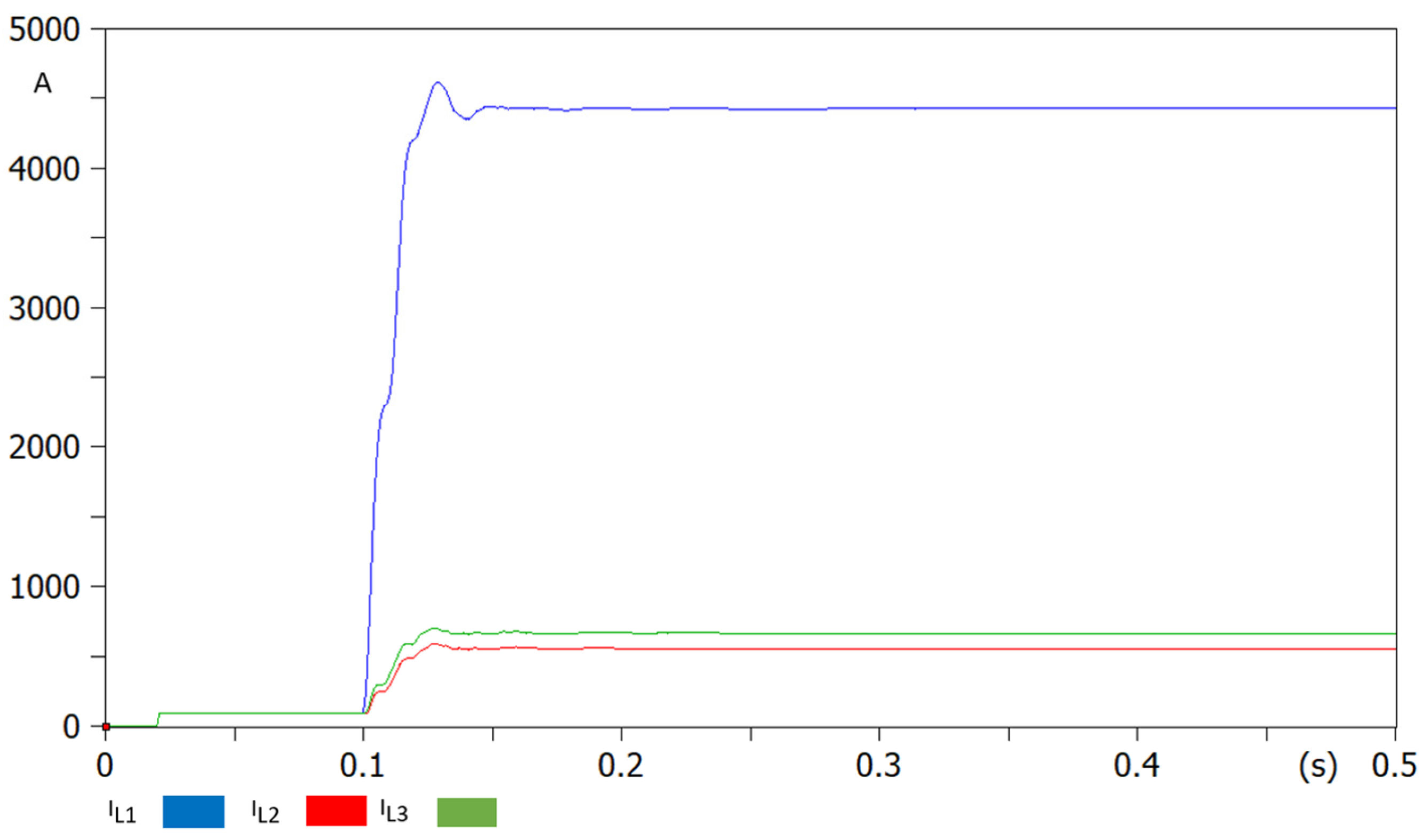
Following the fault configuration illustrated in Figure 8, time-domain simulations are conducted to capture the phase currents and phase-to-ground voltages at the relay location under different arc resistance conditions. 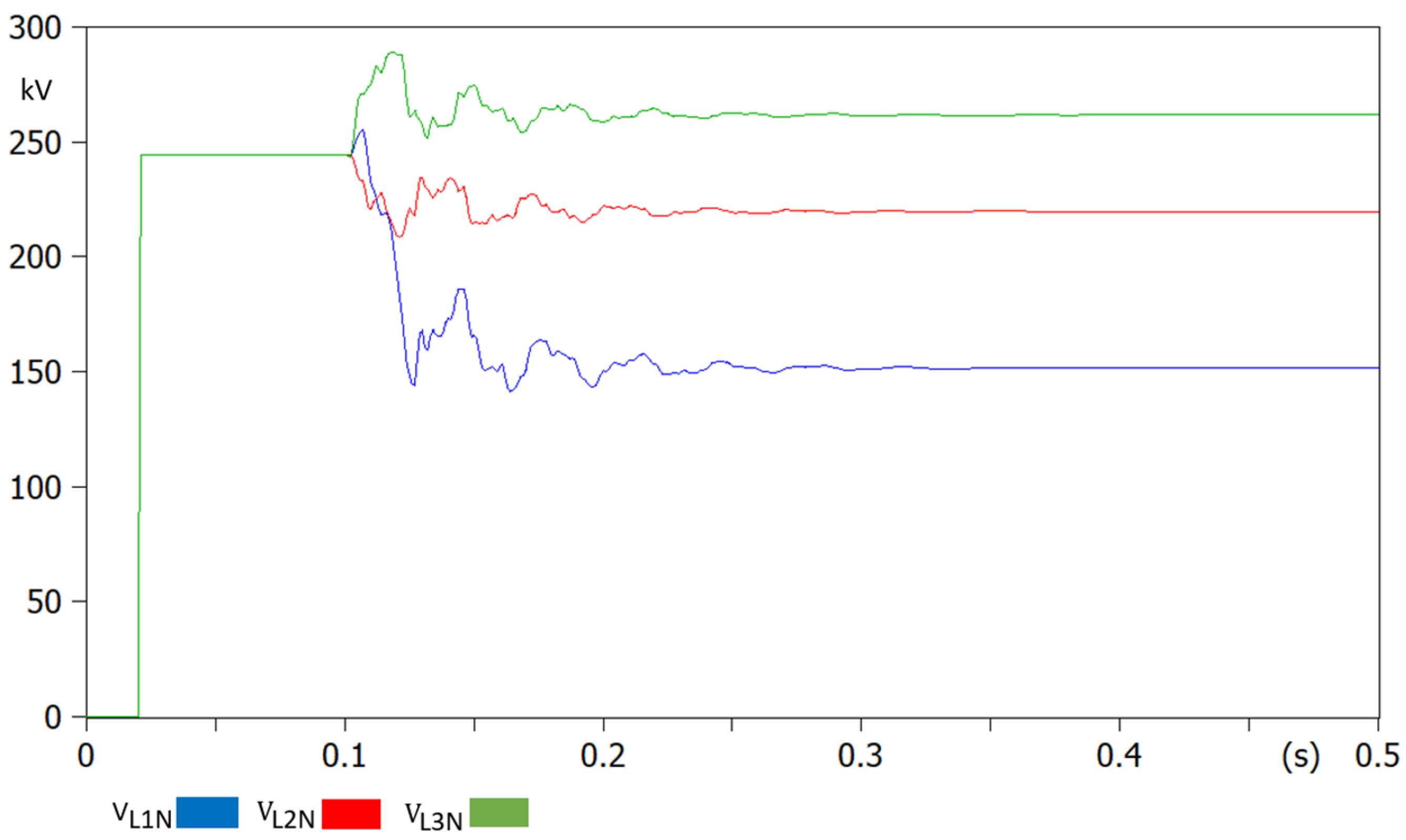The instantaneous phase currents and phase-to-ground voltages for the fault in the first line section with zero arc resistance are shown in Figure 9, while the corresponding RMS values of phase currents and phase-to-ground voltages are presented in Figure 10 and Figure 11, respectively.

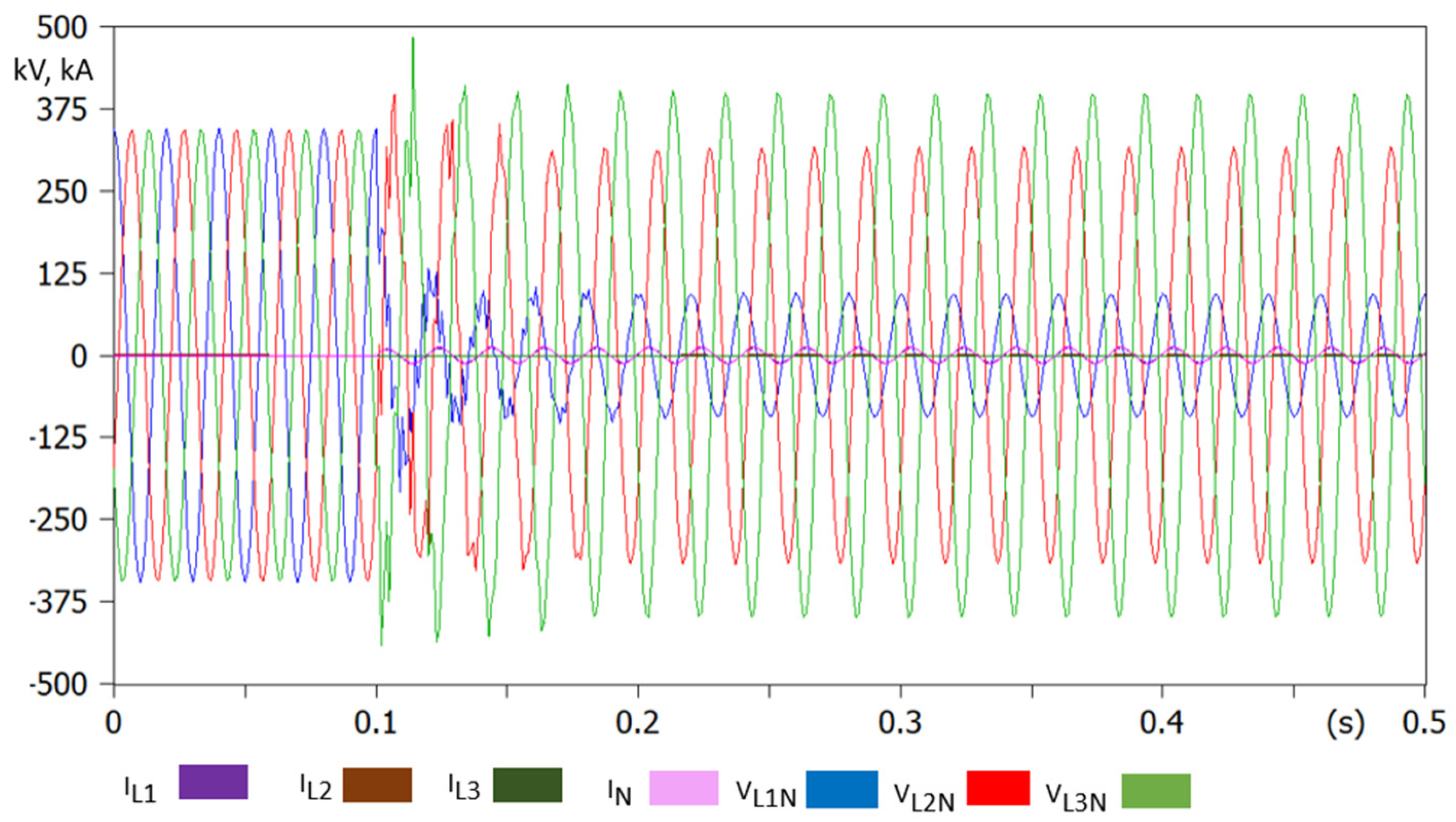
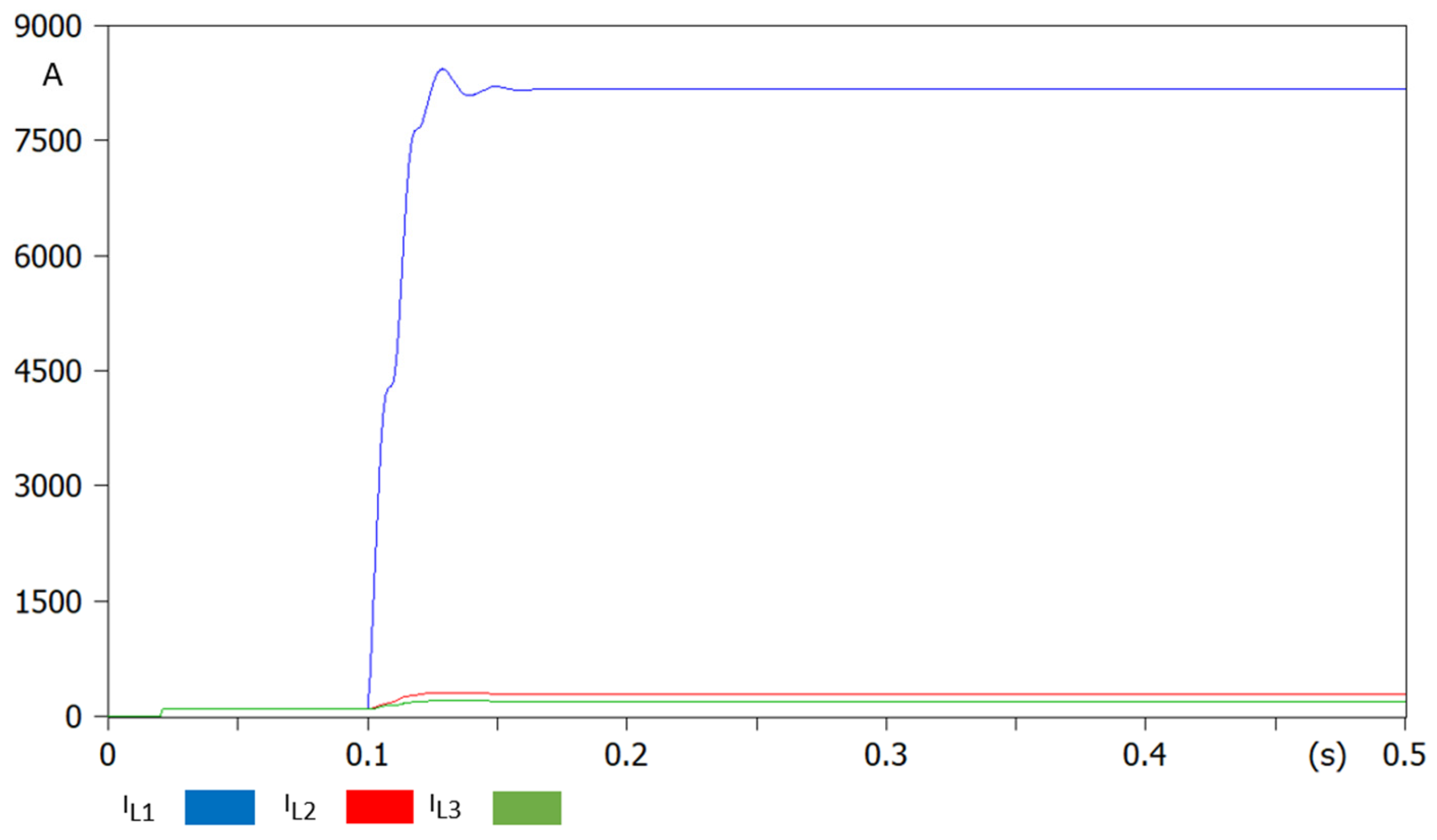
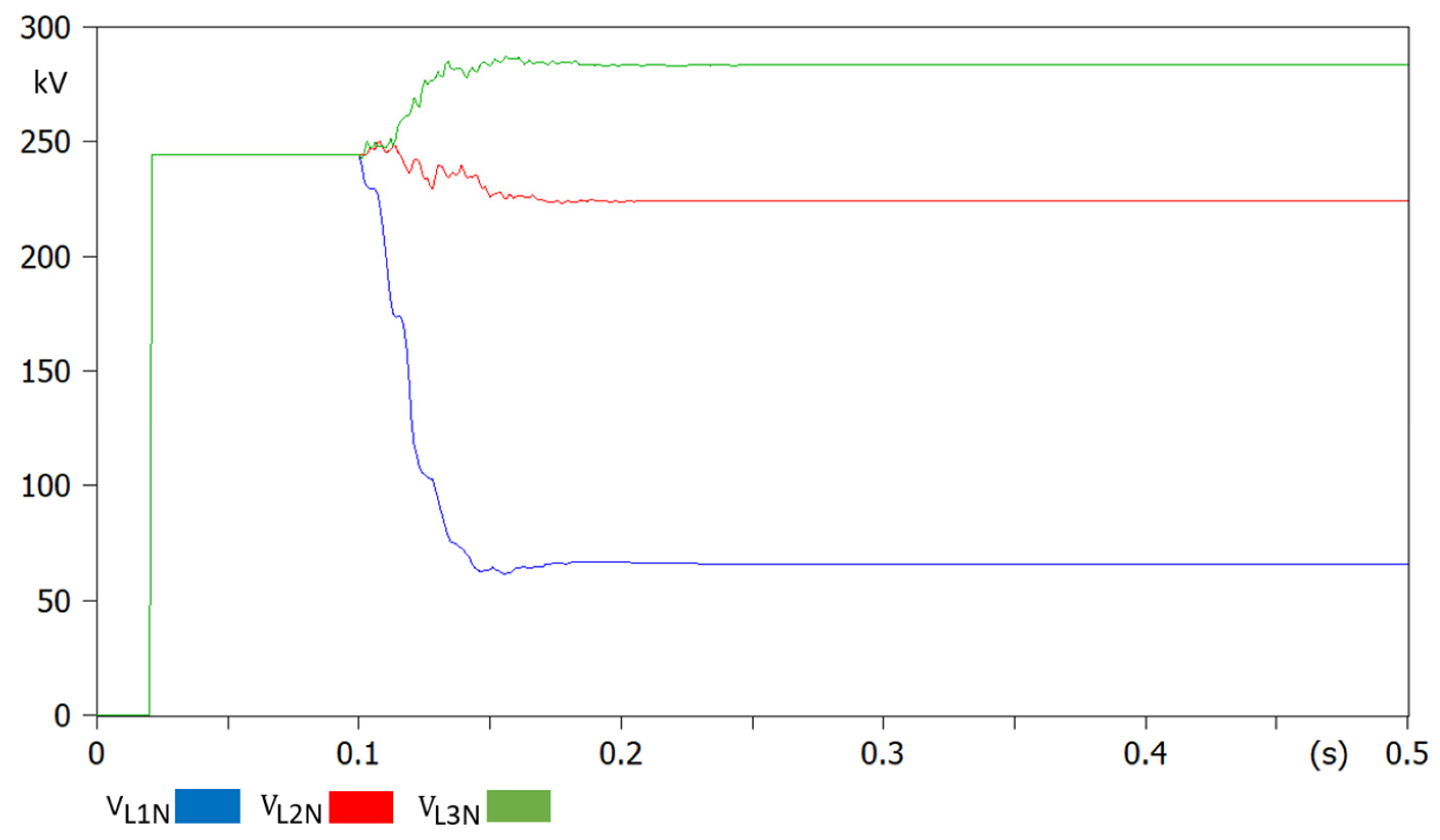
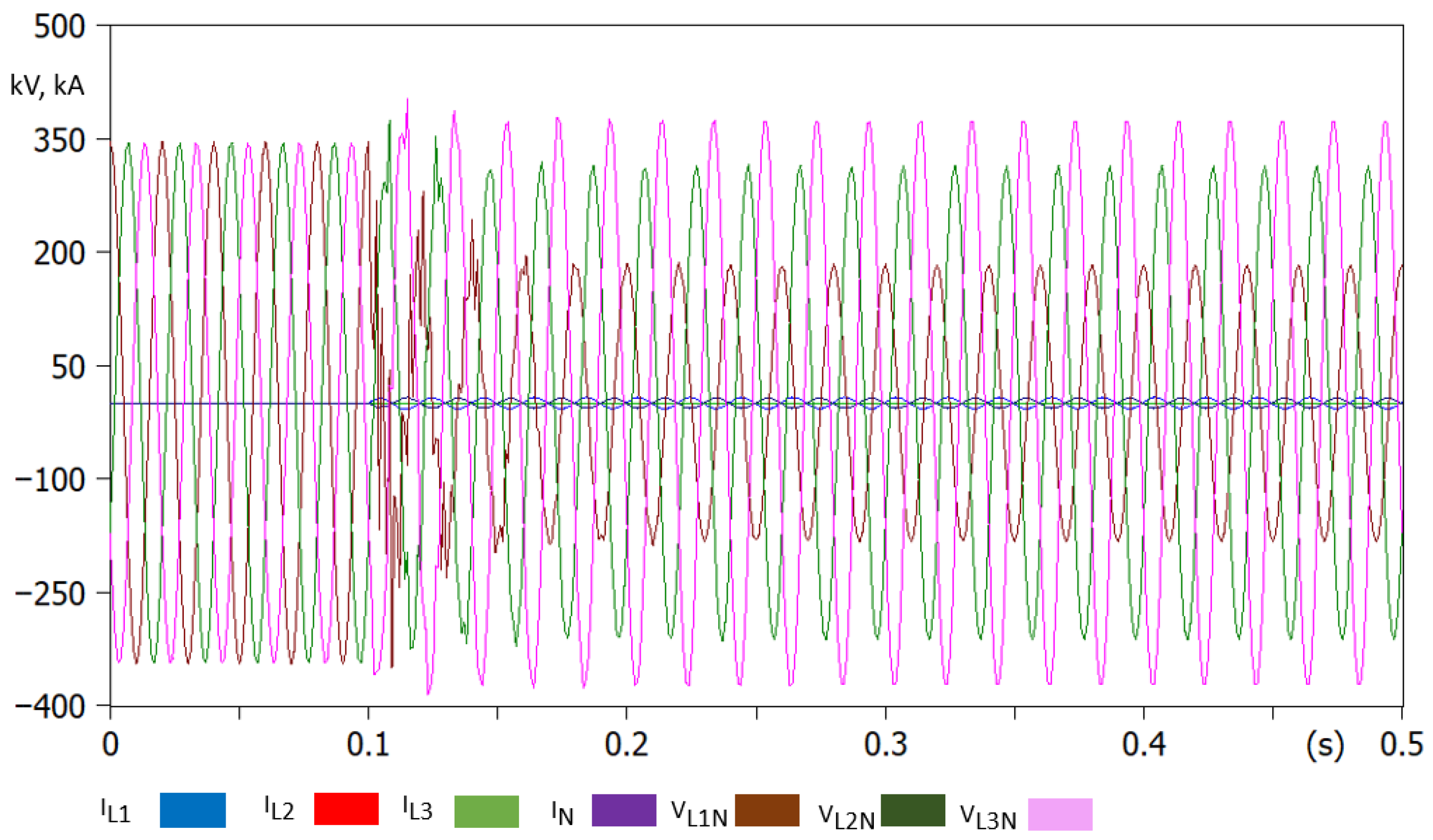
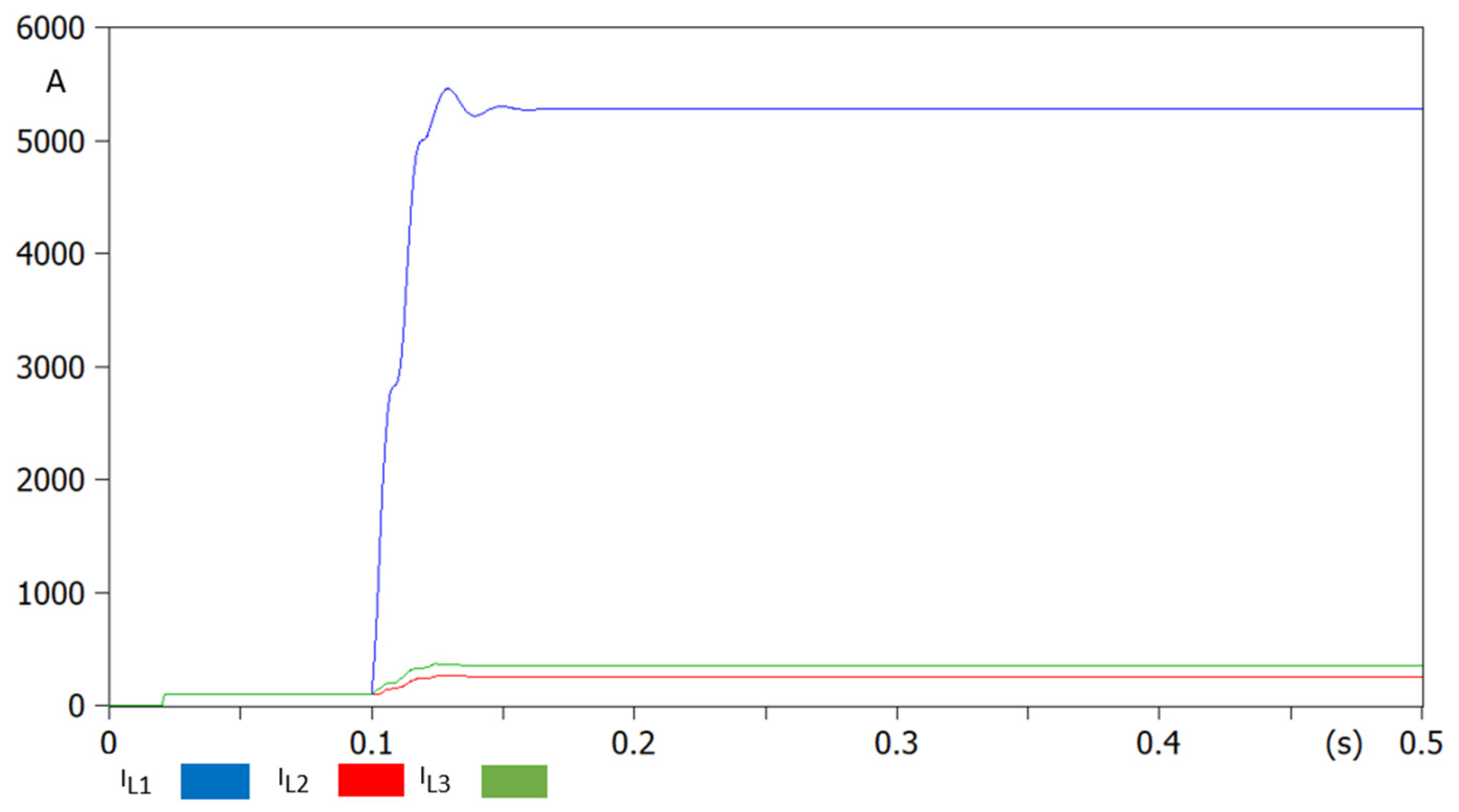
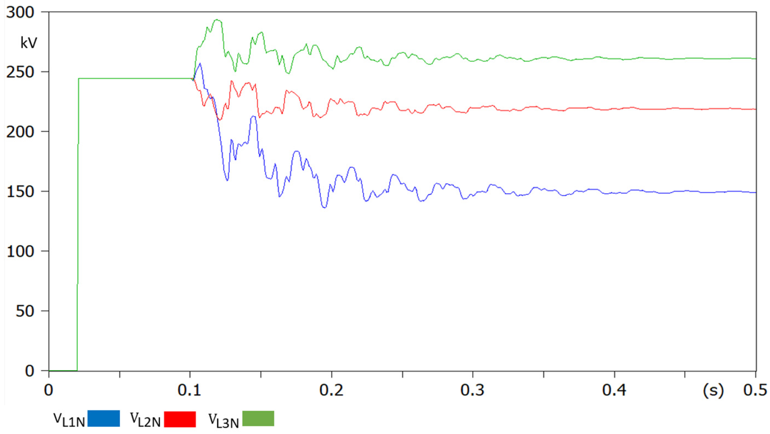
For the non-zero arc resistance case (Rarc = 1 Ω), the instantaneous waveforms of phase currents and phase-to-ground voltages are illustrated in Figure 12, whereas the RMS values of phase currents and phase-to-ground voltages are given in Figure 13 and Figure 14, respectively. These signals constitute the input data for the impedance estimation process of the distance protection algorithms. The comparison between the Rarc = 0 Ω and Rarc = 1 Ω cases enables the evaluation of the robustness of the impedance estimation under varying fault resistance conditions.

3.2. Phase–Ground Fault in the Second Section

The same simulation procedure described in Section 3.1 is applied to an L1–G fault located at the midpoint of the second transmission line section, as illustrated in Figure 15. The instantaneous phase currents and phase-to-ground voltages for the zero arc resistance case are shown in Figure 16, while the corresponding RMS values of phase currents and phase-to-ground voltages are presented in Figure 17 and Figure 18, respectively.

For the non-zero arc resistance case (Rarc = 1 Ω), the instantaneous waveforms are illustrated in Figure 19, whereas the RMS values of phase currents and phase-to-ground voltages are given in Figure 20 and Figure 21, respectively. These signals constitute the input data for the impedance estimation process of the distance protection algorithms and enable a comparative assessment of algorithm performance under different fault resistance conditions.

3.3. Phase–Ground Fault in the Third Section

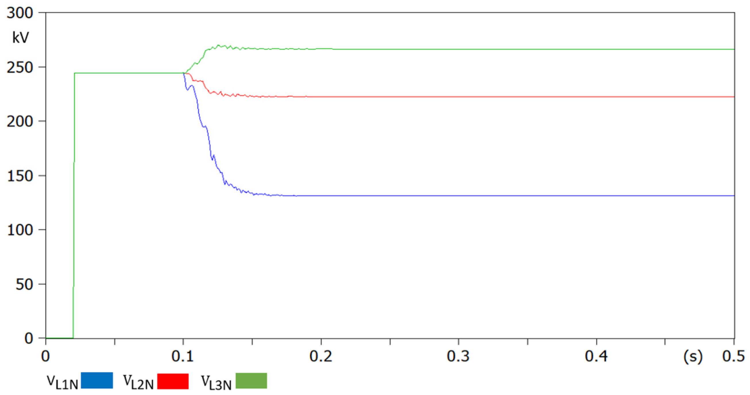
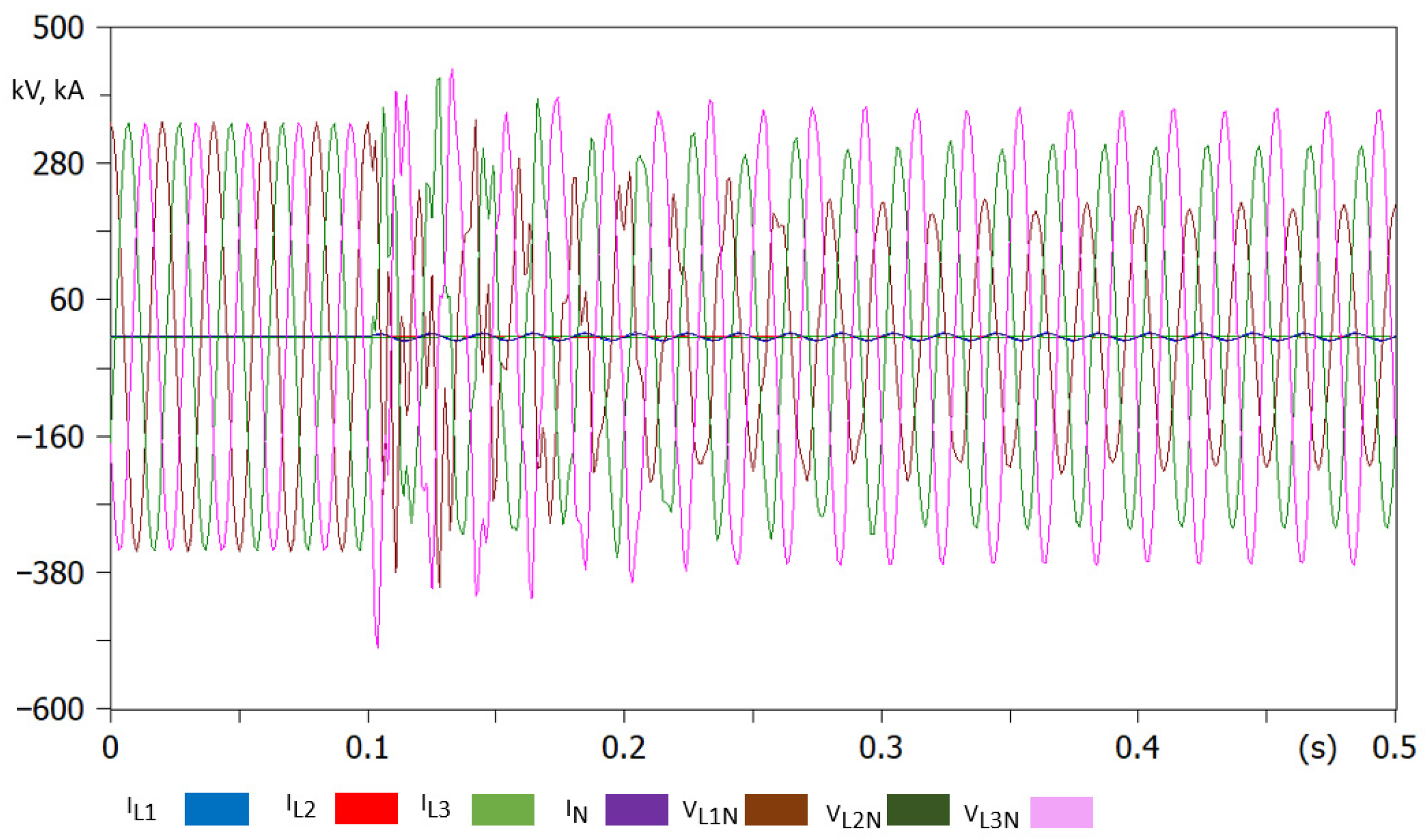
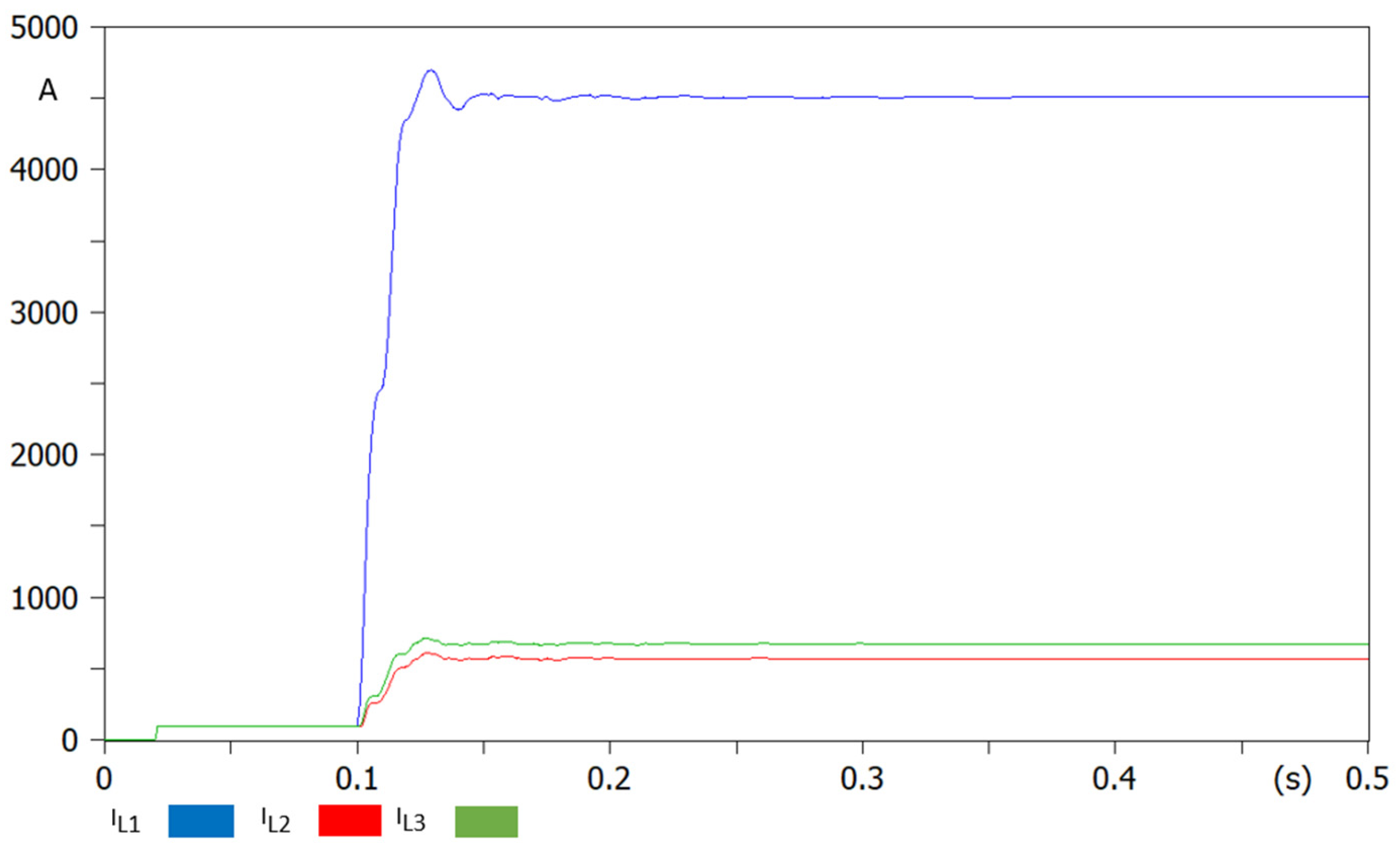
The same simulation procedure described in Section 3.1 is applied to an L1–G fault located at the midpoint of the third transmission line section, as illustrated in Figure 22. The instantaneous phase currents and phase-to-ground voltages for the zero arc resistance case are shown in Figure 23, while the corresponding RMS values of phase currents and phase-to-ground voltages are presented in Figure 24 and Figure 25, respectively.

For the non-zero arc resistance case (Rarc = 1 Ω), the instantaneous waveforms are illustrated in Figure 26, whereas the RMS values of phase currents and phase-to-ground voltages are given in Figure 27 and Figure 28, respectively. These signals constitute the input data for the impedance estimation process of the distance protection algorithms and enable a comparative assessment of algorithm performance under different fault resistance conditions.

4. Performance Comparison Between Classical and Proposed Algorithms

In the implementation of the classical ground distance protection algorithm, the ground compensation factor ${\mathrm{k}}_0$ is computed using Method 2, which is based on the total transmission line impedance. Specifically, the positive- and zero-sequence impedances listed in Table 2 are utilized, and the resulting ${\mathrm{k}}_0$ value is calculated according to Equation (3) using the overall line parameters. The resulting ground compensation factor applied in the classical algorithm, together with the corresponding impedance calculation formulation given by Equation (28), are provided below.

$${\mathrm{k}}_0=0.617-\mathrm{i}0.191=0.618\underset{\_}{/-17.985°}$$

$${\mathrm{Z}}_{\mathrm{Relay}}={\displaystyle \frac{{\mathrm{V}}_{\mathrm{L}1\mathrm{N}}}{{\mathrm{I}}_{\mathrm{L}1}+{\mathrm{I}}_{\mathrm{N}} \times \left(0.618\underset{\_}{/-17.985°}\right)}}$$

(28)

Unlike the classical algorithm, the proposed algorithm employs a separate ${\mathrm{k}}_0$ factor for each line section. The calculated ${\mathrm{k}}_0$ factors for the respective line sections are given below, followed by the corresponding equations applied to each section.

$${\mathrm{k}}_{01}= 0.8316 - \mathrm{i}0.249 =0.868\underset{\_}{/-16.67°}$$

$${\mathrm{k}}_{02}=0.6234-\mathrm{i}0.1949=0.653\underset{\_}{/-17.36°}$$

$${\mathrm{k}}_{03}=-0.212 -\mathrm{i}0.117=0.242\underset{\_}{/-151.073°}$$

$${\mathrm{Z}}_{\mathrm{Relay}}={\displaystyle \frac{{\mathrm{V}}_{\mathrm{L}1\mathrm{N}}}{{\mathrm{I}}_{\mathrm{L}1}+{ \mathrm{I}}_{\mathrm{N}} \times (0.868\underset{\_}{/-16.67°}) }}$$

(29)

$${\mathrm{Z}}_{\mathrm{Relay}}={\displaystyle \frac{{\mathrm{V}}_{\mathrm{L}1\mathrm{N}}}{{\mathrm{I}}_{\mathrm{L}1 }+{\mathrm{I}}_{\mathrm{N}} \times (0.868\underset{\_}{/-16.67°}+0.653\underset{\_}{/-17.36°})}}$$

(30)

$${\mathrm{Z}}_{\mathrm{Relay}}={\displaystyle \frac{{\mathrm{V}}_{\mathrm{L}1\mathrm{N}}}{{\mathrm{I}}_{\mathrm{L}1}+{\mathrm{I}}_{\mathrm{N}} \times (0.868\underset{\_}{/-16.67°}+0.653\underset{\_}{/-17.36°}+0.242\underset{\_}{/-151.073°})}}$$

(31)

To assess the performance of the proposed section-based distance protection algorithm in comparison with the classical ground distance protection approach, a three-step analysis was conducted. First, the phasor quantities measured at the relay location were extracted under steady-state fault conditions. Second, these phasors were used to calculate the apparent impedances using the classical formulation given in Equation (28) and the proposed section-based formulations given in Equations (29)–(31). Finally, the accuracy of the calculated impedances was quantitatively evaluated by comparing them with reference values.

Phasor quantities were extracted from ATP–EMTP at three distinct post-fault instants (200 ms, 250 ms, and 310 ms) to ensure that the analysis is based on steady-state fault conditions and to verify the consistency of the calculated impedances over time. For each fault scenario, the phase voltage, phase current, and residual current phasors measured at the relay location are summarized in

Table 5. The L1 voltage, L1 current and IN phasor measurements recorded by the relay during the fault.

t (ms)		First Fault *		Second Fault		Third Fault
		Rarc = 0 Ω	Rarc = 1 Ω	Rarc = 0 Ω	Rarc = 1 Ω	Rarc = 0 Ω	Rarc = 1 Ω
200	${\mathrm{V}}_{\mathrm{L}1\mathrm{N}}$ (kV)	64.37$\underset{\_}{/0.0°}$	66.44$\underset{\_}{/0.0°}$	129.44$\underset{\_}{/0.0°}$	131.06$\underset{\_}{/0.0°}$	142.49$\underset{\_}{/0.0°}$	149.54$\underset{\_}{/0.0°}$
	${\mathrm{I}}_{\mathrm{L}1}$ (kA)	8.28$\underset{\_}{/-79.1°}$	8.17$\underset{\_}{/-66.1°}$	5.35$\underset{\_}{/-77.6°}$	5.27$\underset{\_}{/-72.4°}$	4.51$\underset{\_}{/-83.2°}$	4.43$\underset{\_}{/-73.1°}$
	${\mathrm{I}}_{\mathrm{N}}$ (kA)	−8.73$\underset{\_}{/-78.0°}$	−8.6$\underset{\_}{/-67.0°}$	−4.80$\underset{\_}{/-80.0°}$	−4.74$\underset{\_}{/-75.3°}$	3.45$\underset{\_}{/-92.3°}$	−3.38$\underset{\_}{/-82.3°}$
250	${\mathrm{V}}_{\mathrm{L}1\mathrm{N}}$ (kV)	63.08$\underset{\_}{/0.0°}$	65.88$\underset{\_}{/0.0°}$	129.31$\underset{\_}{/0.0°}$	130.90$\underset{\_}{/0.0°}$	154.60$\underset{\_}{/0.0°}$	151.88$\underset{\_}{/0.0°}$
	${\mathrm{I}}_{\mathrm{L}1}$ (kA)	8.29$\underset{\_}{/-79.2°}$	8.17$\underset{\_}{/-68.0°}$	5.35$\underset{\_}{/-77.6°}$	5.28$\underset{\_}{/-72.4°}$	4.50$\underset{\_}{/-73.2°}$	4.42$\underset{\_}{/-70.2°}$
	${\mathrm{I}}_{\mathrm{N}}$ (kA)	−8.73$\underset{\_}{/-78.1°}$	−8.6$\underset{\_}{/-67.0°}$	−4.80$\underset{\_}{/-80.4°}$	−4.74$\underset{\_}{/-75.3°}$	3.45$\underset{\_}{/-82.4°}$	−3.38$\underset{\_}{/-79.5°}$
310	${\mathrm{V}}_{\mathrm{L}1\mathrm{N}}$ (kV)	63.48$\underset{\_}{/0.0°}$	66.94$\underset{\_}{/0.0°}$	129.32$\underset{\_}{/0.0°}$	130.91$\underset{\_}{/0.0°}$	151.0$\underset{\_}{/0.0°}$	151.60$\underset{\_}{/0.0°}$
	${\mathrm{I}}_{\mathrm{L}1}$ (kA)	8.29$\underset{\_}{/-79.1°}$	8.17$\underset{\_}{/-68.0°}$	5.35$\underset{\_}{/-77.6°}$	5.28$\underset{\_}{/-72.4°}$	4.50$\underset{\_}{/-77.7°}$	4.42$\underset{\_}{/-71.0°}$
	${\mathrm{I}}_{\mathrm{N}}$ (kA)	−8.73$\underset{\_}{/-78.0°}$	−8.6$\underset{\_}{/-67.0°}$	−4.80$\underset{\_}{/-80.4°}$	−4.74$\underset{\_}{/-75.3°}$	3.44$\underset{\_}{/-86.9°}$	3.38$\underset{\_}{/-80.3°}$

* The slash with underline notation is used to represent the phase angle of phasor quantities.

. The table includes three different fault locations, each evaluated under two fault resistance conditions (Rarc = 0 Ω and 1 Ω). For each location–resistance combination, phasor values are reported at the three post-fault instants, resulting in a comprehensive set of input data for the subsequent impedance calculations.

Using the phasor quantities listed in Table 5, impedance calculations were carried out for both the classical ground distance protection algorithm and the proposed section-based algorithm. The resulting apparent impedance values obtained for each fault case are presented in

Table 6. Impedances Calculated Using the Proposed (${\mathrm{Z}}_{\mathrm{i}}$) and Classical (${\mathrm{Z}}_{\mathrm{ii}}$) Algorithms.

t (ms)		First Fault $(4.03 \mathsf{\Omega }\underset{\_}{/86.56°)}$ *		Second Fault $(14.47 \mathsf{\Omega }\underset{\_}{/85.59°)}$		Third Fault $(22.39 \mathsf{\Omega }\underset{\_}{/85.27°)}$
		Rarc = 0 Ω	Rarc = 1 Ω	Rarc = 0 Ω	Rarc = 1 Ω	Rarc = 0 Ω	Rarc = 1 Ω
200	${\mathrm{Z}}_{\mathrm{i}}$ (Ω)	4.097$\underset{\_}{/86.54°}$	4.30$\underset{\_}{/74.48°}$	14.48$\underset{\_}{/85.43°}$	14.9$\underset{\_}{/80.09°}$	21.07$\underset{\_}{/77.99°}$	22.18$\underset{\_}{/79.02°}$
	${\mathrm{Z}}_{\mathrm{i}\mathrm{i}}$ (Ω)	4.757$\underset{\_}{/85.75°}$	4.96$\underset{\_}{/73.59°}$	15.80$\underset{\_}{/84.84°}$	16.23$\underset{\_}{/79.82°}$	21.99$\underset{\_}{/88.19°}$	23.52$\underset{\_}{/81.72°}$
250	${\mathrm{Z}}_{\mathrm{i}}$ (Ω)	4.012$\underset{\_}{/86.63°}$	4.25$\underset{\_}{/75.48°}$	14.48$\underset{\_}{/85.6°}$	14.86$\underset{\_}{/80.09°}$	22.75$\underset{\_}{/78.71°}$	22.17$\underset{\_}{/74.26°}$
	${\mathrm{Z}}_{\mathrm{i}\mathrm{i}}$ (Ω)	4.66$\underset{\_}{/85.84°}$	4.94$\underset{\_}{/73.68°}$	15.79$\underset{\_}{/84.99°}$	16.19$\underset{\_}{/79.82°}$	23.90$\underset{\_}{/81.85°}$	23.93$\underset{\_}{/78.87°}$
310	${\mathrm{Z}}_{\mathrm{i}}$ (Ω)	4.037$\underset{\_}{/86.53°}$	4.32$\underset{\_}{/75.48°}$	14.48$\underset{\_}{/85.6°}$	14.86$\underset{\_}{/80.09°}$	23.04$\underset{\_}{/86.11°}$	22.27$\underset{\_}{/75.5°}$
	${\mathrm{Z}}_{\mathrm{i}\mathrm{i}}$ (Ω)	4.68$\underset{\_}{/85.78°}$	4.94$\underset{\_}{/74.68°}$	15.79$\underset{\_}{/84.99°}$	16.19$\underset{\_}{/79.82°}$	23.34$\underset{\_}{/86.35°}$	23.88$\underset{\_}{/79.67°}$

* The slash with underline notation is used to represent the phase angle of phasor quantities.

. The table reports the calculated impedances for three different fault locations, each evaluated under two fault resistance conditions (R = 0 Ω and 1 Ω). For each location–resistance combination, impedance estimates obtained using the classical and proposed algorithms are listed at three post-fault instants (200 ms, 250 ms, and 310 ms), enabling a consistent comparison of both methods under identical operating conditions.

To quantitatively evaluate the accuracy of the impedance calculations, the apparent impedance values given in Table 6 were compared with the corresponding reference impedances provided in Table 4. Based on this comparison, percentage magnitude and angle errors were calculated for both the classical and proposed algorithms. The resulting error metrics are presented in

Table 7. Magnitude and angle errors of impedance calculations obtained with the proposed ${(\mathsf{\epsilon }}_{\mathrm{i}})$ and classical $\left({\mathsf{\epsilon }}_{\mathrm{ii}}\right)$ algorithm.

t (ms)	Error	First Fault $(4.03 \mathsf{\Omega }\underset{\_}{/86.56°)}$ *				Second Fault $(14.47 \mathsf{\Omega }\underset{\_}{/85.59°)}$				Third Fault $(22.39 \mathsf{\Omega }\underset{\_}{/85.27°)}$
		Rarc = 0 Ω		Rarc = 1 Ω		Rarc = 0 Ω		Rarc = 1 Ω		Rarc = 0 Ω		Rarc = 1 Ω
		Z	Ang	Z	Ang	Z	Ang	Z	Ang	Z	Ang	Z	Ang
200	${\epsilon }_i$ (%)	1.66	−0.02	6.70	−13.96	0.07	−0.19	2.97	−6.43	−5.90	−8.54	−0.94	−7.33
	${\epsilon }_{ii}$ (%)	18.04	−0.94	23.08	−14.98	9.19	−0.88	12.16	−6.74	−1.79	3.42	5.05	−4.16
250	${\epsilon }_i$ (%)	−0.45	0.08	5.46	−12.80	0.07	0.01	2.70	−6.43	1.61	−7.69	−0.98	−12.91
	${\epsilon }_{ii}$ (%)	15.63	−0.83	22.58	−14.88	9.12	−0.70	11.89	−6.74	6.74	−4.01	6.88	−7.51
310	${\epsilon }_i$ (%)	0.17	−0.03	7.20	−12.80	0.07	0.01	2.70	−6.43	2.90	0.99	−0.54	−11.46
	${\epsilon }_{ii}$ (%)	16.13	−0.90	22.58	−13.72	9.12	−0.70	11.89	−6.74	4.24	1.27	6.65	−6.57

* The slash with underline notation is used to represent the phase angle of phasor quantities.

. The table reports the magnitude and angle error percentages for three different fault locations, each evaluated under two fault resistance conditions (R= 0 Ω and 1 Ω). For each location–resistance combination, the errors associated with the classical and proposed algorithms are listed at three post-fault sampling instants (200 ms, 250 ms, and 310 ms), enabling a detailed assessment of the estimation accuracy and temporal consistency of both approaches.

As shown in Table 7, the proposed section-based algorithm yields lower magnitude error percentages than the classical approach in the vast majority of the investigated fault scenarios, including different fault locations, fault resistance conditions, and post-fault sampling instants. The performance difference becomes particularly significant under resistive fault conditions (Rarc = 1 Ω). For example, at the first fault location and Rarc = 1 Ω, the classical algorithm exhibits magnitude errors exceeding 23% at 200 ms, whereas the proposed algorithm reduces this error to 6.7%. Similarly, at the second fault location under the same fault resistance, the classical method yields a magnitude error of about 12% at 200 ms, compared to less than 3% for the proposed approach. An isolated exception is observed for a solid fault case (Rarc = 0 Ω) at 200 ms, where the classical algorithm exhibits a slightly lower magnitude error. Nevertheless, although the magnitude error of the classical algorithm generally decreases with increasing fault location, reaching its lowest value of −1.79% at the third section, the proposed method maintains superior or comparable accuracy overall, particularly under practical resistive fault conditions.

With regard to angle errors, the proposed algorithm provides improved estimation accuracy for all fault scenarios in the first and second sections. In the third section, the classical algorithm exhibits slightly lower angle errors in some cases; however, the proposed method maintains comparable performance and demonstrates more consistent angle estimation behavior across varying fault resistance conditions and sampling instants.

5. Conclusions

The results of this study demonstrate that the proposed ground distance protection algorithm provides improved accuracy compared to the conventional algorithm for non-uniform transmission lines. Quantitative comparisons indicate that the proposed method significantly reduces impedance magnitude estimation errors in the majority of the simulated fault scenarios and across different fault locations, particularly under resistive fault conditions, when compared to the classical algorithm.

In terms of impedance angle estimation, the proposed algorithm generally yields improved accuracy, especially for faults occurring in the central region of the protected zone and under resistive fault conditions. Although in a limited number of cases the conventional algorithm exhibits slightly lower angle error, the overall angle estimation performance of the proposed method remains comparable or superior, without exhibiting adverse effects on relay reach behavior.

By reducing impedance magnitude estimation errors across the protected zone, the proposed algorithm improves relay reach accuracy compared to the conventional approach. It is also observed that the proposed algorithm may introduce a slight delay in the operation of the distance protection relay within the first protection zone. Nevertheless, this delay is expected to remain within acceptable limits due to ongoing advancements in microprocessor technology.

From an application perspective, the proposed method can be directly implemented in modern numerical distance protection relays with adaptive setting capabilities, particularly for transmission corridors composed of composite or non-uniform line sections. This makes the algorithm suitable for protecting long transmission lines that combine overhead lines and underground cables, which are increasingly deployed in renewable energy integration and urban power systems. Furthermore, the adaptive nature of the proposed approach provides a foundation for future integration with wide-area measurement systems (WAMS) and adaptive protection schemes. It should be noted that the performance evaluation in this study is based on simulation results, and further validation under field conditions will be considered in future work.

References

- Schneider Electric. Micom P441/P442 & P444P441, Numerical Distance Protection Technical Guide. 11 April 2023. Version: 1.0. Available online: https://www.se.com/id/en/download/document/P44x_EN_T_H85/ (accessed on 22 January 2026).
- Schweitzer Engineering Laboratories. Sel 421 Protection, Automation, and Control System Instruction Manual. 14 February 2025. Available online: https://selinc.com/products/421/docs/ (accessed on 22 January 2026).
- Siemens Siprotec 5 7SA87, 7SD87, 7SL87, 7VK87 Technical Manuals, 06.2025, V10.0. Available online: https://support.industry.siemens.com/cs/document/109824501/siprotec-5-7sa87-7sd87-7sl87-7vk87-device-manual?dti=0&lc=en-TR (accessed on 22 January 2026).
- Hitachi Energy. REL670 Transmission Line Distance Protection Technical Manual, Version 2.2 IEC. 23 April 2025. Available online: https://www.hitachienergy.com/products-and-solutions/substation-automation-protection-and-control/products/protection-and-control/relion-product-family/relion-670-series/rel670#tab-tabs-d250564f76-item-fee02e7ec8 (accessed on 22 January 2026).
- Verona, G.E.; Family, U.R. D60 instruction Manual, Production Version: 8.6. 23 October 2024. Available online: https://www.gevernova.com/grid-solutions/resources?prod=d60&type=3 (accessed on 22 January 2026).
- Smith, T.; Zhang, Z.; Lacedonia, M.E.; Pitts, S. Review of application of ground distance protection. In Proceedings of the 2013 66th Annual Conference for Protective Relay Engineers, College Station, TX, USA, 8–11 April 2013; pp. 52–57. [Google Scholar] [CrossRef] [Scilit]
- Bharti, P.; Dehankar, A.; Raut, S.; Unde, S.; Dambhare, S.S. Comparative analysis of fault resistance compensation methods for mutually coupled parallel transmission lines. In Proceedings of the 2016 IEEE 7th Power India International Conference (PIICON), Bikaner, India, 25–27 November 2016. [Google Scholar]
- Eissa, M.M. Ground distance relay compensation based on fault resistance calculation. IEEE Trans. Power Deliv. 2006, 21, 1830–1835. [Google Scholar] [CrossRef] [Scilit]
- Blumschein, J.; Dzienis, C. Compensation of impedance measurement error due to arcing. In Proceedings of the 16th International Conference on Developments in Power System Protection (DPSP 2022), Newcastle, UK, 7–10 March 2022. [Google Scholar]
- Alzyoud, A.R.; Zarour, E.; Jarrar, F.; Arar, A. Modeling and Simulation of Distance Protection for Transmission Lines with Different Grounding Methods. Int. J. Power Syst. 2022, 7, 86–100. [Google Scholar]
- Ghorbani, A.; Mehrjerdi, H. Distance protection with fault resistance compensation for lines connected to PV plant. Int. J. Electr. Power Energy Syst. 2023, 148, 108976. [Google Scholar] [CrossRef] [Scilit]
- Apostolov, A.; Tholomier, D.; Sambasivan, S.; Richards, S. Protection of Double Circuit Transmission Lines. In Proceedings of the 2007 60th Annual Conference for Protective Relay Engineers, College Station, TX, USA, 27–29 March 2007; pp. 85–101. [Google Scholar] [CrossRef] [Scilit]
- O’Donovan, M.; Cowhey, E.; Barry, N.; Connell, J. The Effects of Mutual Coupling Compensation on Distance Protection of Parallel Lines. In Proceedings of the 2020 55th International Universities Power Engineering Conference (UPEC), Turin, Italy, 1–4 September 2020. [Google Scholar]
- Sanaye-Pasand, M.; Jafarian, P. Adaptive protection of parallel transmission lines using combined cross-differential and impedance-based techniques. IEEE Trans. Power Deliv. 2011, 26, 1829–1840. [Google Scholar] [CrossRef] [Scilit]
- Tziouvaras, D.A.; Needs, J. Protection of mixed overhead and underground cable lines. In Proceedings of the 12th IET International Conference on Developments in Power System Protection (DPSP 2014), Copenhagen, Denmark, 31 March–3 April 2014; pp. 12–57. [Google Scholar]
- Zahran, A.D.; Elkalashy, N.I.; Elsadd, M.A.; Kawady, T.A.; Taalab, A.-M.I. Improved ground distance protection for cascaded overhead-submarine cable transmission system. In Proceedings of the 2017 Nineteenth International Middle East Power Systems Conference (MEPCON), Cairo, Egypt, 19–21 December 2017. [Google Scholar]
- Budak, S.; Akbal, B. Comparative Fault Location Estimation by Using Image Processing in Mixed Transmission Lines. Konya J. Eng. Sci. 2021, 8, 62–75. [Google Scholar] [CrossRef] [Scilit]
- Li, B.; Gu, T.; Li, B.; Chen, X.; Wen, W. A New Principle of Distance Protection for the UHV GIL-Overhead Hybrid Line Based on Frequency Domain Lossless Transmission Line Equation. Energies 2019, 12, 4481. [Google Scholar] [CrossRef] [Scilit]
- Aminirad, M.; Mohammad Shahrtash, S. A novel protection and fault location combined algorithm for mixed/hybrid lines. IET Gener. Transm. Distrib. 2022, 16, 2016–2031. [Google Scholar] [CrossRef] [Scilit]
- Abdollahzadeh, H. A distance protection approach for untransposed parallel transmission lines in case of phase-phase-ground inter-circuit faults. Int. J. Electr. Power Energy Syst. 2023, 145, 108623. [Google Scholar] [CrossRef] [Scilit]
Figure 1.
Phase–ground fault. The arrows indicate the phase currents and the short-circuit current (
Figure 2.
Sequence network for a phase to ground fault.
Figure 3.
N-section transmission line model.
Figure 4.
Flowchart of proposed algorithm.
Figure 5.
A 3-section transmission line.
Figure 6.
The impedance plot of the transmission line in the r–x plane is given in