Identification and Mitigation Method of Harmonic Resonance in Offshore Wind Power Systems Based on dq-Domain Modal Analysis

Abstract

Harmonic resonance challenges have intensified in modern power grids, primarily due to the high penetration of converter-based offshore wind energy. Traditional modal analysis methods conducted in the abc reference frame are often constrained by complex coordinate transformations and laborious analytical procedures. Therefore, research into dq-domain modal analysis and mitigation techniques is essential. This paper first elucidates the limitations of conventional modal analysis and outlines the fundamental principles of the dq-domain approach, validating its effectiveness through a three-bus test system. Subsequently, a resonance analysis model for offshore wind systems is established to derive the complete nodal admittance matrix. A dq-domain resonance analysis is then performed, and resonance is mitigated by optimizing the control parameters. Finally, the proposed dq-domain modal analysis method and suppression strategy are validated using a laboratory-scale experimental testbed. The results indicate that the proportional gain of the power control loop (K_PP) significantly influences the system’s resonance modes. Fine-tuning controller parameters via modal analysis provides an active, flexible, and cost-effective solution for resonance suppression.

1. Introduction

Amidst global energy instability and mounting environmental concerns, converter-based offshore wind power has emerged as a major component of the rapidly growing renewable energy landscape [1,2,3,4,5]. However, the interplay between the massive capacitive and inductive components in offshore wind systems can create low-impedance loops at specific frequencies, causing harmonic resonance [6]. Consequential asset damage and mounting service losses seriously undermine the power system’s overall protection and performance [7,8].

The effective analysis of harmonic resonance in offshore wind systems requires accurate modeling of the intricate power coupling and energy exchange between the system’s internal components. Currently, the most prevalent analytical approaches include frequency scanning [9,10,11] and modal analysis [12,13,14,15,16]. Although the former is valued for frequency identification, it is limited by its lack of quantitative insight into component contributions and its high computational cost. Ref. [12] addressed these gaps by introducing modal analysis, which leverages nodal admittance matrix decomposition and participation factors to evaluate resonance. Building on this, Ref. [13] proposed a sensitivity index based on modal impedance for suppression, while the resonant characteristics resulting from grid-tied modules and system impedance were detailed by [14]. The engineering efficacy of modal analysis is well-documented in high-speed railways [15] and wind energy [16,17]. In summary, resonance characteristics are determined by the coupled effects of topology, control strategies, and physical parameters. While [18,19,20] highlighted that interactions between wind farms and converters trigger resonance in subsea cables, Ref. [21] focused on high-frequency oscillations and associated insulation risks, noting that sensitivity analysis of these mechanisms remains limited. Additionally, Ref. [22] examined the impact of converter control on internal resonance. Based on these analytical frameworks, existing research has proposed various mitigation strategies, including control parameter optimization and the control of synchronous current and subsynchronous current injection [23,24].

Nevertheless, existing research is predominantly confined to the abc stationary frame. As offshore wind control architectures evolve, dq-domain control has become the mainstream. Specifically, direct-drive wind turbine systems typically utilize dq-axis decoupled current control for the grid-side converter’s inner loops, with the Phase-Locked Loop (PLL) synchronized in the same rotating frame. Consequently, applying abc-based modal analysis to these systems necessitates tedious coordinate transformations, rendering the workflow inefficient. To address this, there is an urgent need for a novel dq-domain modal analysis methodology that facilitates a more streamlined, scalable, and practicable approach to harmonic resonance identification and suppression.

This study integrates dq-domain modeling with modal analysis theory to develop a novel modal analysis method for investigating harmonic resonance in offshore wind systems. Initially, the drawbacks of conventional modal analysis are discussed, alongside the fundamental principles of the proposed dq-domain approach. A three-node test system is utilized to validate the efficacy of this basic method. Subsequently, a comprehensive resonance analysis model is built, from which the system-wide node admittance matrix is obtained. Furthermore, harmonic resonance analysis is carried out in the dq-domain to examine how various control parameters affect resonance behavior, thereby enabling effective suppression strategies. Ultimately, the proposed analytical and mitigation approaches are validated through the experimental platform.

The main innovations of this paper are summarized as follows:

• Expanded the application dimension of traditional modal analysis methods: Modal analysis is extended from the traditional single-input single-output (SISO) model in the abc stationary frame to a multi-input multi-output (MIMO) model in the dq rotating frame, resolving the issue that traditional methods struggle to characterize the dynamic coupling within control loops.
• Established a full-system dq-domain MIMO nodal admittance model: This paper establishes an offshore wind power model based on a direct-drive wind turbine system, conducts precise modeling of the same, and constructs a MIMO nodal admittance model for the offshore wind power system based on the established model, thereby enabling modal analysis.
• Proposed an active, flexible, and economical resonance suppression method: By reasonably increasing the proportional gain of the power loop (K_PP), the resonance peak can be significantly suppressed, harmonic amplification can be effectively mitigated, and the total harmonic distortion (THD) can be reduced.

2. Limitations of Conventional Modal Analysis and Fundamental Principles of dq-Domain Modal Analysis

2.1. Limitations of Conventional Modal Analysis

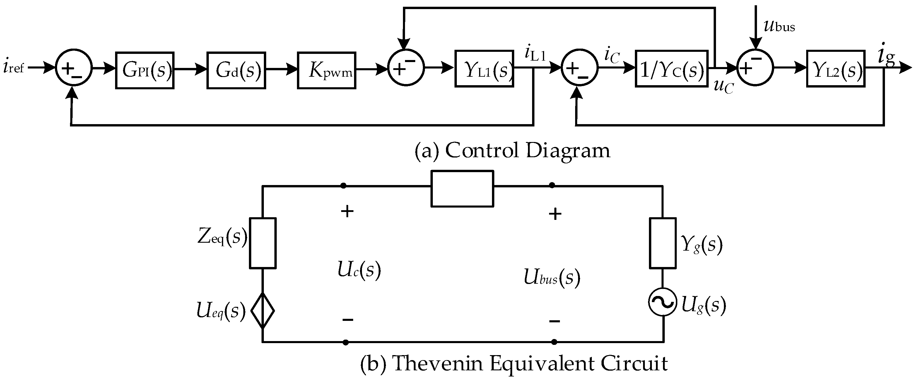
The existence of nonlinear links in offshore wind converters makes the extraction of the nodal admittance matrix extremely difficult. Therefore, in conventional abc-frame modal analysis, researchers often linearize non-linear elements such as the PLL, which yields the control architecture illustrated in Figure 1a. In this figure, Y_L1(s), Y_L2(s), and Y_C(s) correspond to the inverter-side, grid-side, and filter capacitor admittances of the LCL filter, respectively. G_PI(s) represents the transfer function of the inner-loop current PI controller, while G_d(s) and K_pwm characterize the control delay transfer function and the equivalent bridge gain, respectively. Here, s denotes the Laplace variable; K_cp and K_ci are the proportional and integral gains of the current controller; and T_d signifies the control delay.

$$\left\{\begin{array}{l}{Y}_{\mathrm{L}1}(s)=1/s{\mathrm{L}}_1\\ Y_{\mathrm{L}2}(s)=1/s{\mathrm{L}}_2\\ Y_{\mathrm{C}}(s)=s\mathrm{C}\\ G_{\mathrm{PI}}(s)=K_{\mathrm{cp}}+K_{\mathrm{ci}}/s\\ G_{\mathrm{d}}(s)=1/(1+1.5T_{\mathrm{d}}s)\end{array}\right.$$

(1)

To analyze the system harmonic resonance more intuitively, the converter can be represented by a Thévenin equivalent model, as illustrated in Figure 1b. U_eq(s) represents the equivalent voltage of the converter, Z_eq(s) denotes the equivalent impedance of the converter, U_g(s) is the grid voltage, and Y_g(s) is the equivalent grid admittance. Furthermore, it holds that:

$$\left\{\begin{array}{l}{U}_{\mathrm{eq}}(s)={\displaystyle \frac{G_{\mathrm{PI}}{G}_{\mathrm{d}}{K}_{\mathrm{pwm}}{Y}_{\mathrm{L}1}}{Y_{\mathrm{L}1}+Y_{\mathrm{C}}+G_{\mathrm{PI}}{G}_{\mathrm{d}}{K}_{\mathrm{pwm}}{Y}_{\mathrm{L}1}{Y}_{\mathrm{C}}}}{i}_{\mathrm{ref}}\\ {\mathrm{Z}}_{\mathrm{eq}}(s)={\displaystyle \frac{1+G_{\mathrm{PI}}{G}_{\mathrm{d}}{K}_{\mathrm{pwm}}{Y}_{\mathrm{L}1}}{Y_{\mathrm{L}1}+Y_{\mathrm{C}}+G_{\mathrm{PI}}{G}_{\mathrm{d}}{K}_{\mathrm{pwm}}{Y}_{\mathrm{L}1}{Y}_{\mathrm{C}}}}\end{array}\right.$$

(2)

Figure 1b employs a SISO impedance model for the equivalent representation of the non-linear converter. While this simplifies the construction of the system nodal admittance matrix, the method is inherently an approximation of the system’s dynamic characteristics. Since the model neglects the influence of the PLL, the asymmetric dynamic responses of the d and q axes cannot be fully characterized within the admittance matrix, which may subsequently compromise the accuracy of the resonance analysis results.

2.2. Fundamental Principles of dq-Domain Modal Analysis

For a three-phase system with n + 1 nodes operating stably at a given operating point, it can be represented as:

$$\{{\mathit{U}}_1(h),{\mathit{U}}_2(h),\dots ,{\mathit{U}}_i(h),\dots ,{\mathit{U}}_n(h)\}$$

(3)

where U_i(h)(i = 0, 1, …n) is the node voltage matrix of the i-th node at the h-th harmonic, defined as U_i(h) = [U_id(h) U_iq(h)] ^T.

When a small disturbance vector [Δi₁ Δi₂ … Δi_j … Δi_n]^T is injected into the network nodes, the node voltage variations are as follows:

$$\underset{\mathit{U}}{\underbrace{\left[\begin{array}{c}\mathrm{\Delta }{\mathit{u}}_1\\ \mathrm{\Delta }{\mathit{u}}_2\\ ⋮\\ \mathrm{\Delta }{\mathit{u}}_i\\ ⋮\\ \mathrm{\Delta }{\mathit{u}}_n\end{array}\right]}}=\underset{{\mathit{Y}}^{-1}}{\underbrace{\left[\begin{array}{cccccc}{\mathit{Y}}_{11}^{-1}& {\mathit{Y}}_{12}^{-1}& \dots & {\mathit{Y}}_{1j}^{-1}& \dots & {\mathit{Y}}_{1n}^{-1}\\ {\mathit{Y}}_{21}^{-1}& {\mathit{Y}}_{22}^{-1}& \dots & {\mathit{Y}}_{2j}^{-1}& \dots & {\mathit{Y}}_{2n}^{-1}\\ ⋮& ⋮& & ⋮& & ⋮\\ {\mathit{Y}}_{i1}^{-1}& {\mathit{Y}}_{i2}^{-1}& \dots & {\mathit{Y}}_{ij}^{-1}& \dots & {\mathit{Y}}_{in}^{-1}\\ ⋮& ⋮& & ⋮& & ⋮\\ {\mathit{Y}}_{n1}^{-1}& {\mathit{Y}}_{n2}^{-1}& \dots & {\mathit{Y}}_{nj}^{-1}& \dots & {\mathit{Y}}_{nn}^{-1}\end{array}\right]}}\underset{\mathit{I}}{\underbrace{\left[\begin{array}{c}\mathrm{\Delta }{\mathit{i}}_1\\ \mathrm{\Delta }{\mathit{i}}_2\\ ⋮\\ \mathrm{\Delta }{\mathit{i}}_j\\ ⋮\\ \mathrm{\Delta }{\mathit{i}}_n\end{array}\right]}}$$

(4)

where the variables U, I, and Y in the equation are defined as the dq-frame small-signal bus voltage vector, the current injection vector, and the network admittance matrix. The corresponding elements Δu_i, Δi_j, and Y_ij are given by:

$${\mathit{Y}}_{ij}=\left[\begin{array}{cc}{Y}_{ij,a}& Y_{ij,b}\\ Y_{ij,c}& Y_{ij,d}\end{array}\right],\mathrm{\Delta }{\mathit{u}}_i=\left[\begin{array}{c}\mathrm{\Delta }{u}_{i,d}\\ \mathrm{\Delta }{u}_{i,q}\end{array}\right],\mathrm{\Delta }{\mathit{i}}_j=\left[\begin{array}{c}\mathrm{\Delta }{i}_{j,d}\\ \mathrm{\Delta }{i}_{j,q}\end{array}\right]$$

(5)

The matrix Y can be decomposed as follows:

$$\mathit{Y}=\mathit{L}\mathit{\Lambda }\mathit{T}$$

(6)

The right and left eigenvectors are encapsulated in matrices T and L, respectively, where L = T⁻¹. Furthermore, the eigenvalues of the system form the diagonal elements of matrix Λ.

Substituting (6) into (4) yields:

$$\mathit{T}\mathit{U}={\mathit{\Lambda }}^{-1}\mathit{T}\mathit{I}$$

(7)

By designating U_mode = TU and I_mode = TI as the modal voltage and current vectors, respectively, the aforementioned formulation takes the simpler form:

$${\mathit{U}}_{\mathrm{mode}}={\mathit{\Lambda }}^{-1}{\mathit{I}}_{\mathrm{mode}} \mathrm{or}\left[\begin{array}{c}{U}_{\mathrm{mode}1}\\ U_{\mathrm{mode}2}\\ ⋮\\ U_{\mathrm{mode}2n}\end{array}\right]=\left[\begin{array}{cccc}{\lambda }_1^{-1}& 0& 0& 0\\ 0& {\lambda }_2^{-1}& 0& 0\\ 0& 0& \ddots & 0\\ 0& 0& 0& {\lambda }_{2n}^{-1}\end{array}\right]\left[\begin{array}{c}{I}_{\mathrm{mode}1}\\ I_{\mathrm{mode}2}\\ ⋮\\ I_{\mathrm{mode}2n}\end{array}\right]$$

(8)

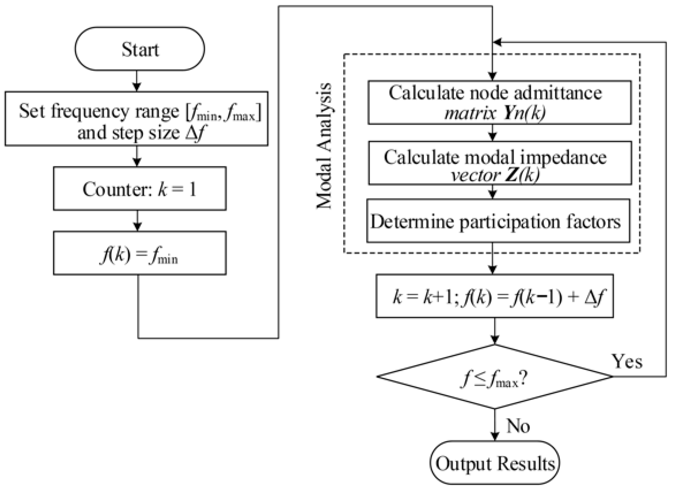
In the equation, the reciprocal of the eigenvalues represents an impedance property and is defined as the modal impedance. When an eigenvalue of a certain mode becomes extremely small or approaches zero, its corresponding modal impedance increases dramatically. This implies that in this mode, a negligible injection current I_mode can be amplified into a significantly high modal voltage U_mode. Since the modes are decoupled from each other (the off-diagonal elements are zero), resonance in one mode does not affect the others. Within the context of harmonic resonance, the critical mode corresponds to the minimum eigenvalue, with its related left and right eigenvectors termed critical eigenvectors. By scanning the magnitudes of the eigenvalues, the specific modes with resonance risks in the system can be identified directly and clearly. The flowchart of modal analysis in the dq reference frame is shown in Figure 2.

2.3. Validation of the Proposed Modal Analysis Method

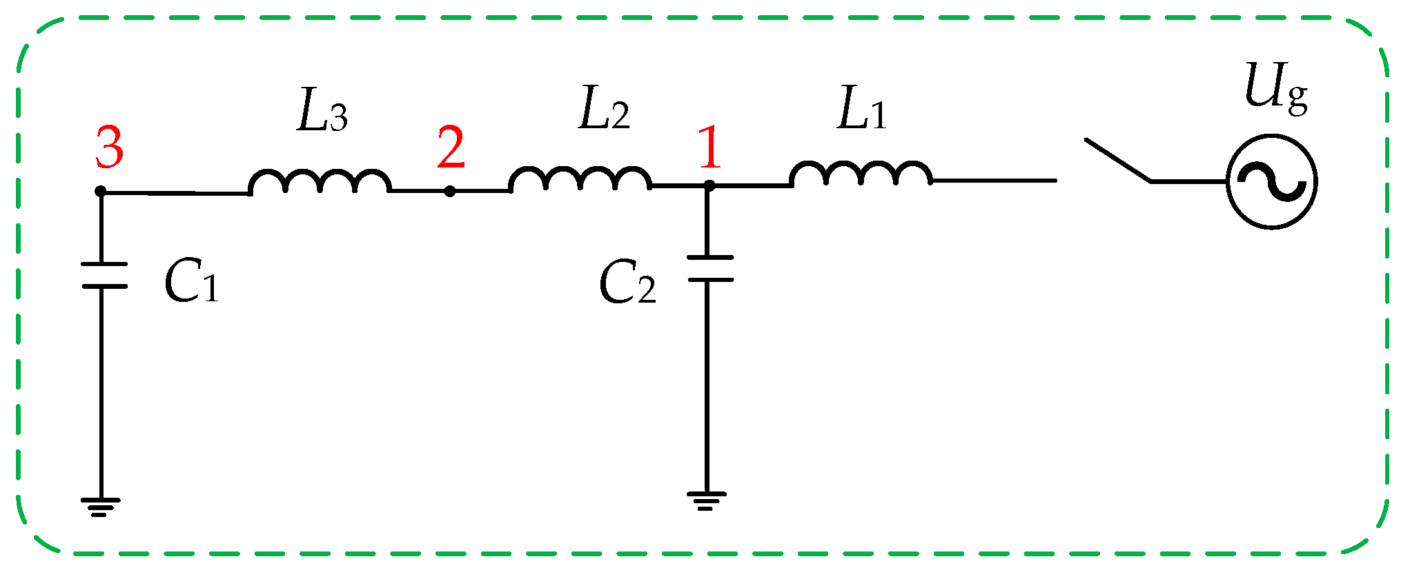
A three-node test system was established, as shown in Figure 3. This system consists of three nodes where harmonic resonance can be observed. Modal analysis was performed on the system, and the results were compared with Simulink simulation results for validation.

First, the node admittance matrix Y_n3 is established. The corresponding matrix is given as follows:

$$\begin{array}{l}{\mathit{Y}}_{n3}=\left[\begin{array}{ccc}{Y}_{11}& Y_{12}& Y_{13}\\ Y_{21}& Y_{22}& Y_{23}\\ Y_{31}& Y_{32}& Y_{33}\end{array}\right]\\ =\left[\begin{array}{ccc}{Y}_{L1}+Y_{L2}+Y_{C1}& -Y_{L2}& 0\\ -Y_{L2}& Y_{L2}+Y_{L3}& -Y_{L3}\\ 0& -Y_{L3}& Y_{L3}+Y_{C2}\end{array}\right]\end{array}$$

(9)

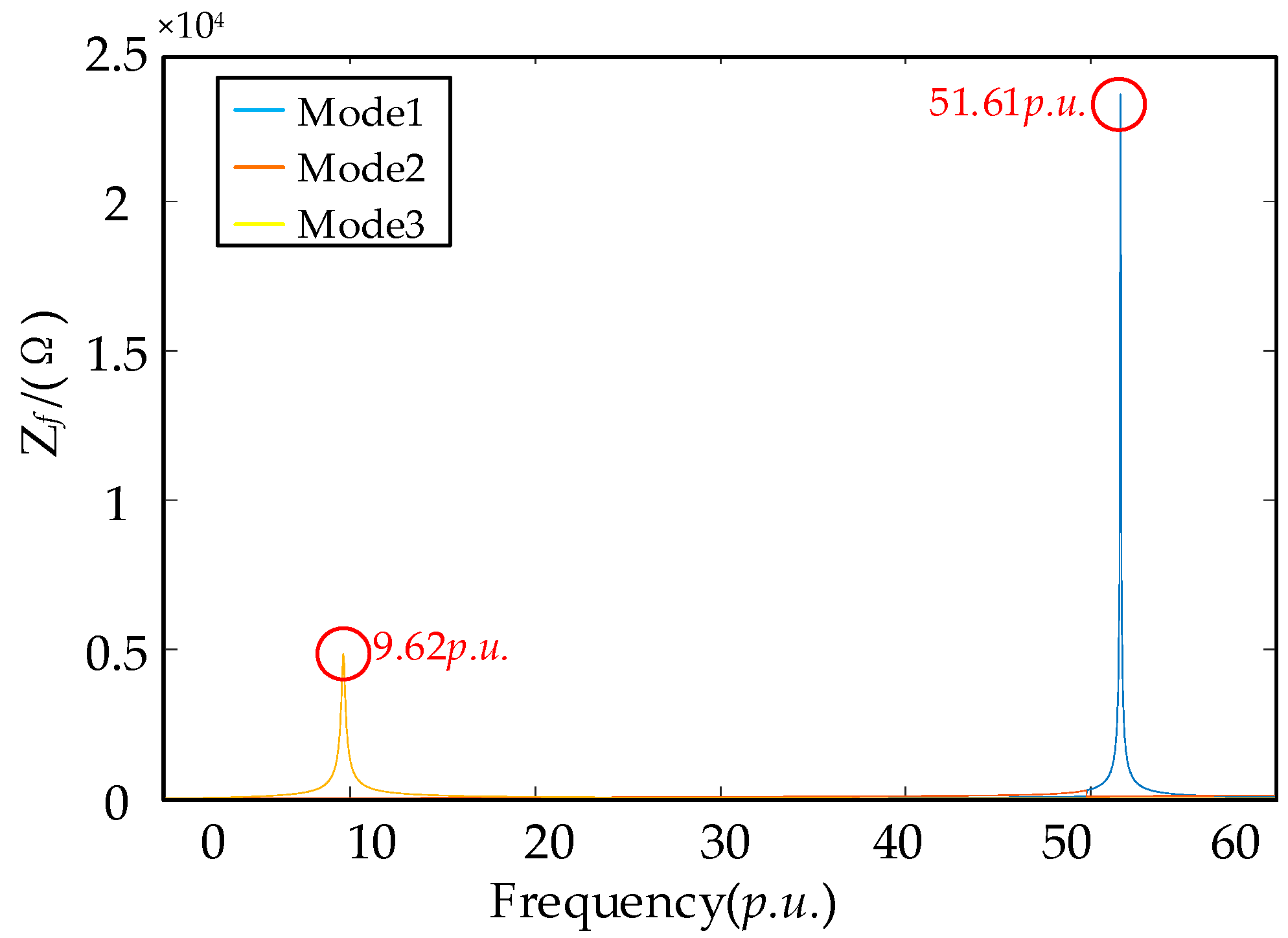
By performing eigenvalue decomposition, the modal impedance curves and the corresponding maximum modal impedance curve were obtained, as shown in Figure 4. Two resonance points occurred at 9.62 p.u. and 51.61 p.u. Modal analysis indicates that the resonance frequency of 9.6 p.u. corresponded to Mode 3, while 51.6 p.u. corresponded to Mode 1.

For the sake of clarity, all frequency values in this paper are expressed in per-unit (p.u.) system. The base frequency was chosen as the fundamental grid frequency f_base = 50 Hz. Therefore, the per-unit frequency was defined as f_p.u. = f/f_base.

By representing the corresponding Y_L1, Y_L2, Y_L3, Y_C1, and Y_C2 in the dq frame, the node admittance matrix Y_n3dq in the dq coordinate system is obtained.

$$\begin{array}{l}{\mathit{Y}}_{n3dq}=\left[\begin{array}{ccc}{\mathit{Y}}_{11dq}& {\mathit{Y}}_{12dq}& {\mathit{Y}}_{13dq}\\ {\mathit{Y}}_{21dq}& {\mathit{Y}}_{22dq}& {\mathit{Y}}_{23dq}\\ {\mathit{Y}}_{31dq}& {\mathit{Y}}_{32dq}& {\mathit{Y}}_{33dq}\end{array}\right]\\ =\left[\begin{array}{ccc}{\mathit{Y}}_{L1dq}+{\mathit{Y}}_{L2dq}+{\mathit{Y}}_{C1dq}& -{\mathit{Y}}_{L2dq}& 0\\ -{\mathit{Y}}_{L2dq}& {\mathit{Y}}_{L2dq}+{\mathit{Y}}_{L3dq}& -{\mathit{Y}}_{L3dq}\\ 0& -{\mathit{Y}}_{L3dq}& {\mathit{Y}}_{L3dq}+{\mathit{Y}}_{C2dq}\end{array}\right]\end{array}$$

(10)

where:

$$\begin{array}{l}{\mathit{Y}}_{Lndq}={\mathit{Z}}_{Lndq}^{-1}\\ {\mathit{Y}}_{Cndq}={\mathit{Z}}_{Cndq}^{-1}\\ {\mathit{Z}}_{Lndq}=\left[\begin{array}{cc}{R}_n+s{L}_n& -\omega L_n\\ \omega L_n& R_n+s{L}_n\end{array}\right]\\ {\mathit{Z}}_{Cndq}=\left[\begin{array}{cc}{R}_n+s{C}_n& -\omega L_n\\ \omega L_n& R_n+s{C}_n\end{array}\right]\end{array}$$

(11)

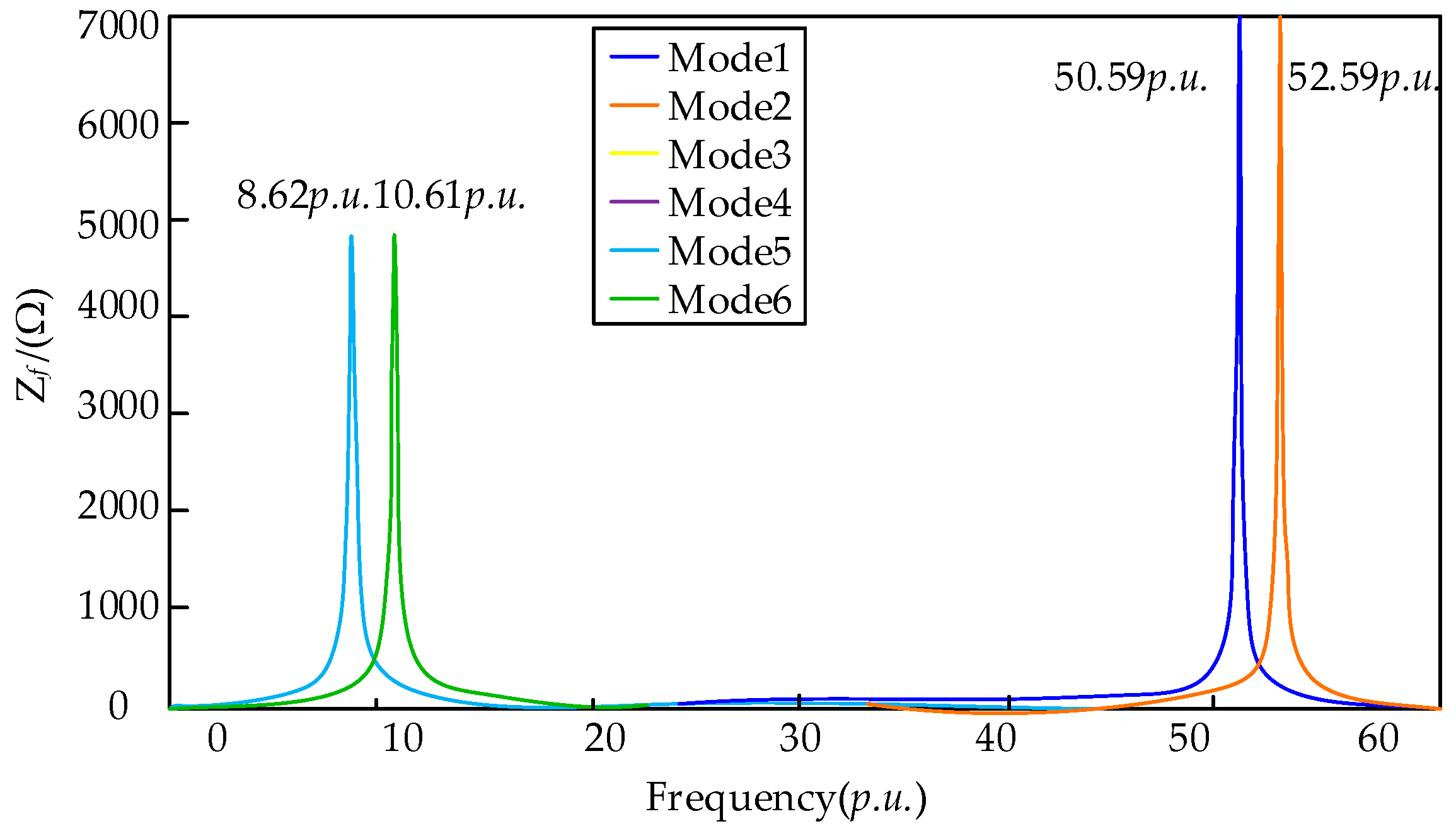
The node admittance matrix is of a 6 × 6 size. Modal analysis was performed on this matrix, and the results are presented in Figure 5. As illustrated in the figure, four distinct peaks can be observed. Specifically, the peaks at 8.62 p.u. and 10.62 p.u. corresponded to 9.62 ± 1 p.u., while the peaks at 50.61 p.u. and 52.61 p.u. corresponded to 51.61 ± 1 p.u. respectively. This phenomenon is a direct consequence of the dq transformation. Suppose that a resonance exists in the stationary abc frame at a frequency f_res. This implies the presence of a voltage or current component that can be expressed as cos(ω_rest), where ω_res = 2πf_res. When this signal is transformed into the dq frame, it is effectively multiplied by a rotation factor, cos(ω_gridt), where ω_grid = 2π × 50 Hz (the fundamental grid frequency). According to trigonometric identities, the transformed signal will contain two new frequency components:

• cos((ω_res − ω_grid) t), which corresponds to the frequency f_res − 50 Hz;
• cos((ω_res + ω_grid) t), which corresponds to the frequency f_res + 50 Hz.

Due to the characteristics of the dq transformation, the resonance frequency f_res in the stationary frame (abc frame) appears as shifted components f_dq = f_res ± f_grid in the rotating frame (dq frame). In the per-unit system, this corresponds to f_{dq_p.u.} = f_{res_p.u.} ± 1. Therefore, a single-point resonance at frequency f_res in the stationary frame will split into two sideband frequencies, f_res − 1 p.u. and f_res + 1 p.u., when observed in the dq frame rotating synchronously at 50 Hz. Consequently, the resonance frequencies identified in the figure corresponded to 9.615 p.u. and 51.59 p.u., which are consistent with the modal analysis results in the abc frame. This confirms the accuracy of the proposed modal analysis method in the dq coordinate system.

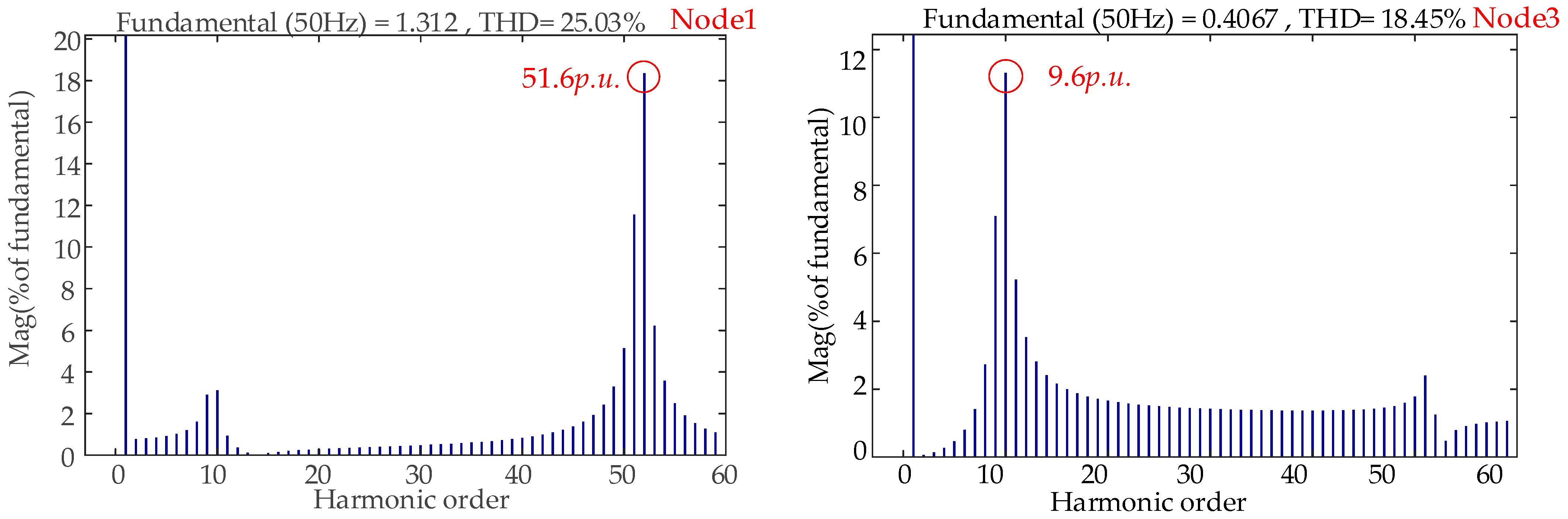
A three-bus system was constructed in Simulink, and Fast Fourier Transform (FFT) analysis was performed on the bus voltages, yielding the results shown in Figure 6. The figure indicates a resonance at 51.6 p.u. for Bus 1 and a resonance at 9.98 p.u. for Bus 3. These findings align with the aforementioned modal analysis results, providing further validation for the proposed modal analysis method in the dq frame.

The results of the traditional modal analysis method based on the abc frame were compared with those of the proposed modal analysis method based on the dq frame as well as with the Simulink FFT analysis results, and the data obtained are shown in

Table 1. Comparison of the two modal analysis methods with the FFT analysis results.

	FFT Analysis (p.u.)	Modal Analysis Method Based on the abc Frame		Modal Analysis Method Based on the dq Frame
		Resulting Per-Unit Resonance Frequencies (p.u.)	Error Relative to the FFT Analysis Results	Resulting Per-Unit Resonance Frequencies (p.u.)	Error Relative to the FFT Analysis Results
Resonance frequencies 1	51.6	51.61	0.019%	51.59	0.019%
Resonance frequencies 2	9.6	9.62	0.208%	9.615	0.156%

. The data indicate that both methods yielded small errors and were relatively accurate. However, the modal analysis method based on the dq frame is capable of performing modal analysis on models that cannot be characterized under the abc frame, thereby expanding the application scope of modal analysis methods. This paper presents a generalized framework for dq-domain modal analysis. This approach is universally applicable to any topology amenable to dq-domain modeling, making it a valuable asset for engineering applications.

3. Modeling of Offshore Wind Power Systems for Resonance Analysis

3.1. Configuration of an Offshore Wind Power System with Direct-Drive Wind Turbines

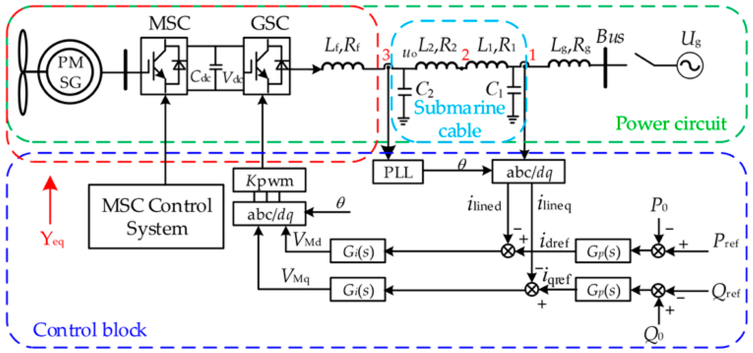
The PQ control configuration, as presented in Figure 7, integrates an outer power control loop and an inner current loop along with a PLL. Its corresponding power stage features several key elements, including the direct-drive wind turbine, the machine-side converter (MSC) and the grid-side converter (GSC) units, submarine cables, and the external utility grid.

In Figure 7, V_dc represents the DC-link voltage; MSC and GSC denote the Machine-Side Converter and Grid-Side Converter, respectively; C_dc is the DC-link capacitor. L₂/L₃ and R₂/R₃ represent the line inductance and its equivalent resistance, while L_f and R_f are the filter inductance and its parasitic resistance. The equivalent grid inductance and resistance are denoted by L_g and R_g. C_f and R_d represent the filter capacitance and its damping resistance. P₀/Q₀ and P_ref/Q_ref are the actual and reference values of the inverter’s active/reactive power output, respectively. i_dref and i_qref are the d-axis and q-axis current reference values for the inverter output. This paper employed dq-axis decoupling control, where G_p(s) = K_ps + K_is/s and G_c(s) = K_pc + K_ic/s serve as the PI regulators for the power loop and current loop, respectively.

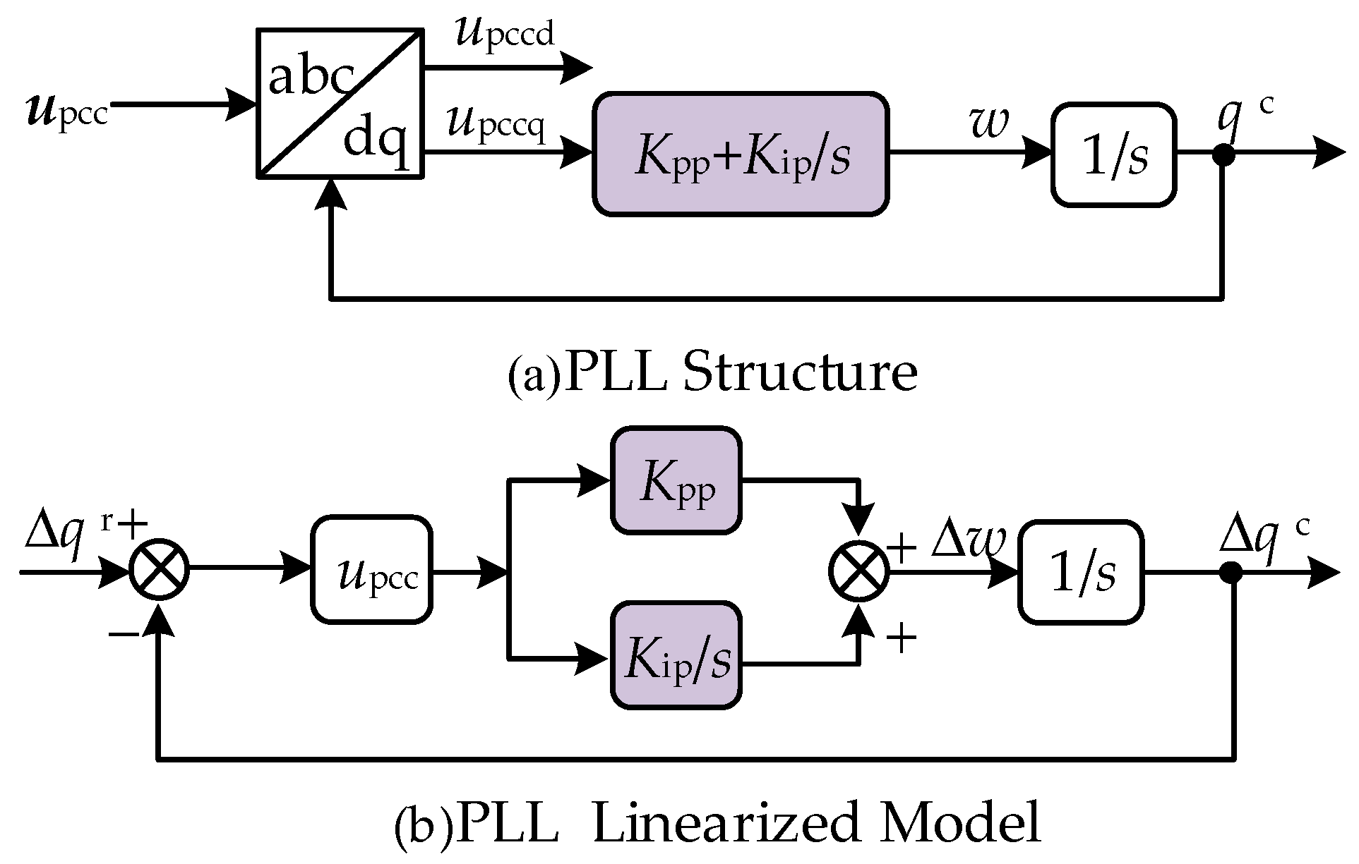
To maintain synchronization with the power grid, this paper adopted the Synchronous Reference Frame Phase-Locked Loop (SRF-PLL) based on the synchronous reference frame to track the grid voltage. Its basic structure and linearized model are shown in Figure 8, and the corresponding output characteristics are as follows:

$$G_{\theta }(s)={\displaystyle \frac{\mathrm{\Delta }\theta }{\mathrm{\Delta }{V}_{\mathrm{tq}}^s}}={\displaystyle \frac{G_{\mathrm{PLL}}(s)}{s+V_{\mathrm{td}0}{G}_{\mathrm{PLL}}(s)}}$$

(12)

where G_PLL(s) = K_pp + K_ip/s; ω₀ and ω are the rated and actual angular velocities, respectively; and V_td0 is the steady-state value of the d-axis terminal voltage.

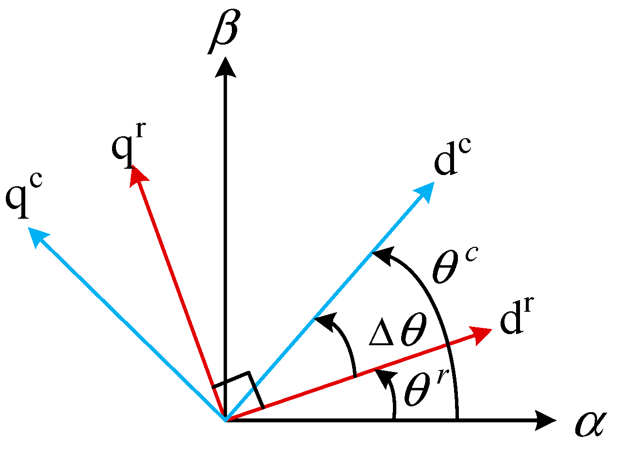
When voltage fluctuations occur at the PCC, the PLL tracks these changes, leading to an angular deviation Δθ between the PLL output phase angle θ^c and the actual phase angle θ^s of the PCC voltage, i.e., θ^c = θ^s +Δθ. The schematic of the relationship between synchronous and control reference frames are shown in Figure 9. The conversion that relates the variables x^s in the system’s synchronous frame to their counterparts x^c in the control domain can be stated as:

$$\left\{\begin{array}{l}\mathrm{\Delta }{x}_{\mathrm{d}}^{\mathrm{c}}=\mathrm{\Delta }{x}_{\mathrm{d}}^{\mathrm{s}}+\mathrm{\Delta }\theta x_{\mathrm{q}0}^{\mathrm{s}}\hfill \\ \mathrm{\Delta }{x}_{\mathrm{q}}^{\mathrm{c}}=\mathrm{\Delta }{x}_{\mathrm{q}}^{\mathrm{s}}-\mathrm{\Delta }\theta x_{\mathrm{d}0}^{\mathrm{s}}\hfill \end{array}\right.$$

(13)

Substituting (12) into (13) yields:

$$\left\{\begin{array}{l}\mathrm{\Delta }{x}_d^c=\mathrm{\Delta }{x}_d^s+{\displaystyle \frac{G_{PLL}(s)x_{q0}^s}{s+V_{td0}{G}_{PLL}(s)}}\mathrm{\Delta }{V}_{tq}^s\hfill \\ \mathrm{\Delta }{x}_q^c=\mathrm{\Delta }{x}_q^s-{\displaystyle \frac{G_{PLL}(s)x_{d0}^s}{s+V_{td0}{G}_{PLL}(s)}}\mathrm{\Delta }{V}_{tq}^s\hfill \end{array}\right.$$

(14)

3.2. Small-Signal Mathematical Modeling of Direct-Drive Wind Turbines with PQ Control

The dq-axis components of the wind turbine’s modulation voltage, $e_{\mathrm{d}\mathrm{r}\mathrm{e}\mathrm{f}}^{\mathrm{c}}$ and $e_{\mathrm{q}\mathrm{r}\mathrm{e}\mathrm{f}}^{\mathrm{c}}$, are obtained from the current loop. In the control reference frame, they are expressed as:

$$\left\{\begin{array}{c}{e}_{dref}^c=G_c\left(s\right)\left(i_{\mathrm{L}1dref}^c-i_{\mathrm{L}1d}^c\right)\\ e_{qref}^c=G_c\left(s\right)\left(i_{\mathrm{L}1qref}^c-i_{\mathrm{L}1\mathrm{q}}^c\right)\end{array}\right.$$

(15)

where the dq-axis current variables for the grid-side inductor L₁ are designated as $i_{\mathrm{L}1\mathrm{d}}^{\mathrm{c}}$ and $i_{\mathrm{L}\mathrm{1}\mathrm{q}\mathrm{f}}^{\mathrm{c}}$; their associated control references are given by $i_{\mathrm{L}\mathrm{d}\mathrm{r}\mathrm{e}\mathrm{f}}^{\mathrm{c}}$ and $i_{\mathrm{L}\mathrm{q}\mathrm{r}\mathrm{e}\mathrm{f}}^{\mathrm{c}}$. Performing small-signal analysis yields:

$$\left\{\begin{array}{c}\mathrm{\Delta }{e}_{dref}^c=G_c\left(s\right)\left(\mathrm{\Delta }{i}_{\mathrm{L}1dref}^c-\mathrm{\Delta }{i}_{\mathrm{L}1d}^c\right)\\ \mathrm{\Delta }{e}_{qref}^c=G_c\left(s\right)\left(\mathrm{\Delta }{i}_{\mathrm{L}1qref}^c-\mathrm{\Delta }{i}_{\mathrm{L}1\mathrm{q}}^c\right)\end{array}\right.$$

(16)

The modulation voltage in the control reference frame Δ$e_{\mathrm{r}\mathrm{e}\mathrm{f}}^{\mathrm{c}}$ is identical to that in the SRF Δ$e_{\mathrm{r}\mathrm{e}\mathrm{f}}^{\mathrm{s}}$. In the SRF, the wind turbine’s output voltage Δe is correlated with the controller’s voltage reference $e_{\mathrm{r}\mathrm{e}\mathrm{f}}^{\mathrm{s}}$ according to:

$$\left\{\begin{array}{l}\mathrm{\Delta }{\mathit{e}}_{r\mathit{e}f}^s=\mathrm{\Delta }{\mathit{e}}_{r\mathit{e}f}^c\\ \mathrm{\Delta }\mathit{e}=\mathrm{\Delta }{\mathit{e}}_{r\mathit{e}f}^s{G}_{d\mathit{e}}\left(s\right)\end{array}\right.$$

(17)

where G_de(s) is the delay element, which is ignored in this study and assumed to be 1.

Transforming (16) into the synchronous reference frame yields:

$$\left\{\begin{array}{cc}\hfill \mathrm{\Delta }{e}_{dref}^s& =G_c(s)\mathrm{\Delta }{i}_{L1dref}^c-G_c(s)\left(\mathrm{\Delta }{i}_{\mathrm{L}1\mathrm{d}}^s+I_{\mathrm{L}1q0}\mathrm{\Delta }\theta \right)-E_{q0}\mathrm{\Delta }\theta \hfill \\ & =G_c(s)\mathrm{\Delta }{i}_{L1dref}^c-G_c(s)\mathrm{\Delta }{i}_{\mathrm{L}1\mathrm{d}}^s+\left[-G_c(s)I_{\mathrm{L}1q0}-E_{q0}\right]\mathrm{\Delta }\theta \hfill \\ \mathrm{\Delta }{e}_{qref}^s& =G_c(s)\mathrm{\Delta }{i}_{L1qref}^c-G_c(s)\left(\mathrm{\Delta }{i}_{\mathrm{L}1\mathrm{q}}^s-I_{\mathrm{L}1d0}\mathrm{\Delta }\theta \right)+E_{d0}\mathrm{\Delta }\theta \hfill \\ & =G_c(s)\mathrm{\Delta }{i}_{L1qref}^c-G_c(s)\mathrm{\Delta }{i}_{\mathrm{L}1\mathrm{q}}^s+\left[G_c(s)I_{\mathrm{L}1d0}+E_{d0}\right]\mathrm{\Delta }\theta \hfill \end{array}\right.$$

(18)

where h_θ1 and h_θ2 are defined as:

$$\left\{\begin{array}{l}{h}_{\theta 1}=-G_c(s)I_{L1q0}-E_{q0}\\ h_{\theta 2}=G_c(s)I_{L1d0}+E_{d0}\end{array}\right.$$

(19)

Substituting into (18) yields:

$$\left\{\begin{array}{c}\mathrm{\Delta }{e}_d^s=G_{de}(s)G_c(s)\mathrm{\Delta }{i}_{L1dref}^c-G_{de}(s)G_c(s)\mathrm{\Delta }{i}_{\mathrm{L}1\mathrm{d}}^s+G_{de}(s)h_{\theta 1}\mathrm{\Delta }\theta \\ \mathrm{\Delta }{e}_q^s=G_{de}(s)G_c(s)\mathrm{\Delta }{i}_{L1qref}^c-G_{de}(s)G_c(s)\mathrm{\Delta }{i}_{\mathrm{L}1\mathrm{q}}^s+G_{de}(s)h_{\theta 2}\mathrm{\Delta }\theta \end{array}\right.$$

(20)

The expression for the wind turbine’s power loop is:

$$\left\{\begin{array}{c}\mathrm{\Delta }{i}_{L1dref}^c=G_{pp}\left(\mathrm{\Delta }{P}_{ref}-\mathrm{\Delta }{P}_e\right)\\ \mathrm{\Delta }{i}_{L1qref}^c=G_{pq}\left(\mathrm{\Delta }{Q}_e-\mathrm{\Delta }{Q}_{ref}\right)\end{array}\right.$$

(21)

where G_pp and G_pq denote the dq-axis parameters of the power loop PI controller.

The perturbation equations for active and reactive power are given by:

$$\left\{\begin{array}{l}\mathrm{\Delta }{P}_e={\displaystyle \frac{3}{2}}{F}_L\left(\mathrm{\Delta }{u}_{oq}{I}_{oq0}+U_{oq0}\mathrm{\Delta }{i}_{oq}+\mathrm{\Delta }{u}_{od}{I}_{od0}+U_{od0}\mathrm{\Delta }{i}_{od}\right)\\ \mathrm{\Delta }{Q}_e={\displaystyle \frac{3}{2}}{F}_L\left(\mathrm{\Delta }{u}_{oq}{I}_{od0}+U_{oq0}\mathrm{\Delta }{i}_{od}-\mathrm{\Delta }{u}_{od}{I}_{oq0}-U_{od0}\mathrm{\Delta }{i}_{oq}\right)\end{array}\right.$$

(22)

Substituting (21) and (22) into (20), neglecting the power reference perturbations and setting U_oq = 0, yields:

$$\left\{\begin{array}{l}\mathrm{\Delta }{e}_d^s=-G_{de}{G}_c{G}_{pp}{\displaystyle \frac{3}{2}}{F}_L\left(U_{od0}\mathrm{\Delta }{i}_{\mathrm{o}\mathrm{d}}^s+\mathrm{\Delta }{u}_{\mathrm{o}\mathrm{q}}^s{I}_{oq0}\right)-G_{de}{G}_c\mathrm{\Delta }{i}_{\mathrm{L}1\mathrm{d}}^s\\ -G_{de}{G}_c{G}_{pp}{\displaystyle \frac{3}{2}}{F}_L{I}_{od0}\mathrm{\Delta }{u}_{\mathrm{o}\mathrm{d}}^s+G_{de}{h}_{\theta 1}\mathrm{\Delta }\theta \\ \mathrm{\Delta }{e}_q^s=G_{de}{G}_c{G}_{pq}{\displaystyle \frac{3}{2}}{F}_L\left(-\mathrm{\Delta }{u}_{\mathrm{o}\mathrm{d}}^s{I}_{oq0}-U_{od0}\mathrm{\Delta }{i}_{\mathrm{o}\mathrm{q}}^s\right)-G_{de}{G}_c\mathrm{\Delta }{i}_{\mathrm{L}1\mathrm{q}}^s\\ +G_{de}{G}_c{G}_{pq}{\displaystyle \frac{3}{2}}{F}_L{I}_{od0}\mathrm{\Delta }{u}_{\mathrm{o}\mathrm{q}}^s+G_{de}{h}_{\theta 2}\mathrm{\Delta }\theta \end{array}\right.$$

(23)

The relationship for the power circuit in the synchronous reference frame is:

$$\left\{\begin{array}{c}\mathrm{\Delta }{e}_d^s=Z_{fd}\mathrm{\Delta }{i}_{od}^s-Z_{fq}\mathrm{\Delta }{i}_{oq}^s+\mathrm{\Delta }{u}_{\mathrm{od}}^s\\ \mathrm{\Delta }{e}_q^s=Z_{fq}\mathrm{\Delta }{i}_{od}^s+Z_{fd}\mathrm{\Delta }{i}_{oq}^s+\mathrm{\Delta }{u}_{\mathrm{oq}}^s\end{array}\right.$$

(24)

The association between the turbine output current and the grid current is defined by:

$$\begin{array}{l}\left\{\begin{array}{l}\mathrm{\Delta }{i}_{L3d}^s=\mathrm{\Delta }{i}_{\mathrm{od}}^s+\omega C_2\mathrm{\Delta }{u}_{\mathrm{oq}}^s\\ \mathrm{\Delta }{i}_{L3q}^s=\mathrm{\Delta }{i}_{\mathrm{oq}}^s-\omega C_2\mathrm{\Delta }{u}_{\mathrm{od}}^s\end{array}\right.\\ \left\{\begin{array}{l}\mathrm{\Delta }{i}_{L1d}^s=\mathrm{\Delta }{i}_{L3d}^s+\omega C_2\mathrm{\Delta }{u}_{\mathrm{oq}}^s\\ \mathrm{\Delta }{i}_{L1q}^s=\mathrm{\Delta }{i}_{L3q}^s-\omega C_2\mathrm{\Delta }{u}_{\mathrm{od}}^s\end{array}\right.\end{array}$$

(25)

By substituting (25) into (23) and eliminating Δ$i_{\mathrm{L}\mathrm{d}}^{\mathrm{s}}$ and Δ$i_{\mathrm{L}\mathrm{q}}^{\mathrm{s}}$, we obtain:

$$\left\{\begin{array}{l}\mathrm{\Delta }{e}_d^s=G_{kk1}\mathrm{\Delta }{u}_{od}^s+G_{kk2}\mathrm{\Delta }{u}_{oq}^s-G_{kkp}\mathrm{\Delta }{i}_{od}^s+G_{de}{h}_{\theta 1}{\displaystyle \frac{F_{\mathrm{PLL}}(s)}{s+U_{od0}{F}_{\mathrm{PLL}}(s)}}\mathrm{\Delta }{u}_{\mathit{oq}}^{\mathrm{s}}\\ \mathrm{\Delta }{e}_q^s=-G_{kk3}\mathrm{\Delta }{u}_{od}^s+G_{kk4}\mathrm{\Delta }{u}_{oq}^s-G_{kkq}\mathrm{\Delta }{i}_{oq}^s+G_{de}{h}_{\theta 2}{\displaystyle \frac{F_{\mathrm{PLL}}(s)}{s+U_{od0}{F}_{\mathrm{PLL}}(s)}}\mathrm{\Delta }{u}_{\mathit{oq}}^{\mathrm{s}}\end{array}\right.$$

(26)

where G_kk1, G_kk2, G_kk3, G_kk4, G_kkp, and G_kkq are defined as follows:

$$\left\{\begin{array}{l}{G}_{kk1}=-G_{de}{G}_c{G}_{pp}{\displaystyle \frac{3}{2}}{F}_L{I}_{od0}\\ G_{kk2}=-G_{de}{G}_c{G}_{pp}{\displaystyle \frac{3}{2}}{F}_L{I}_{oq0}\\ G_{kk3}=G_{de}{G}_c{G}_{pq}{\displaystyle \frac{3}{2}}{F}_L{I}_{oq0}\\ G_{kk4}=G_{de}{G}_c{G}_{pq}{\displaystyle \frac{3}{2}}{F}_L{I}_{od0}\\ G_{kkp}=G_{de}{G}_c+G_{de}{G}_c{G}_{pp}{\displaystyle \frac{3}{2}}{F}_L{U}_{od0}\\ G_{kkq}=G_{de}{G}_c+G_{de}{G}_c{G}_{pq}{\displaystyle \frac{3}{2}}{F}_L{U}_{od0}\end{array}\right.$$

(27)

Combining the above equations yields the relationship between the wind turbine output voltage and current as follows:

$$\left\{\begin{array}{l}\mathrm{\Delta }{i}_{od}^s{G}_{H1}+\mathrm{\Delta }{i}_{oq}^s{G}_{H2}=\mathrm{\Delta }{u}_{\mathrm{od}}^s{G}_{D1}+\mathrm{\Delta }{u}_{\mathrm{oq}}^s{G}_{D2}\\ \mathrm{\Delta }{i}_{od}^s{G}_{H3}+\mathrm{\Delta }{i}_{oq}^s{G}_{H4}=\mathrm{\Delta }{u}_{\mathrm{od}}^s{G}_{D3}+\mathrm{\Delta }{u}_{\mathrm{oq}}^s{G}_{D4}\end{array}\right.$$

(28)

where G_H1, G_H2, G_H3, G_H4, G_D1, G_D2, G_D3, and G_D4 are defined as follows:

$$\begin{array}{l}\left\{\begin{array}{l}{G}_{H1}=\left(Z_{fd}+G_{kkp}\right)\left(s+U_{\mathit{od}0}{G}_{\mathrm{PLL}}(s)\right)\\ G_{H2}=-Z_{fq}\left(s+U_{\mathit{od}0}{G}_{\mathrm{PLL}}(s)\right)\\ G_{H3}=Z_{fq}\left(s+U_{\mathit{od}0}{G}_{\mathrm{PLL}}(s)\right)\\ G_{H4}=\left(G_{kkq}+Z_{fd}\right)\left(s+U_{\mathit{od}0}{G}_{\mathrm{PLL}}(s)\right)\end{array}\right.\\ \left\{\begin{array}{l}{G}_{D1}=\left(G_{kk1}-G_{uu}-1\right)\left(s+U_{\mathit{od}0}{G}_{\mathrm{PLL}}(s)\right)\\ G_{D2}=G_{de}{h}_{\theta 1}{F}_{\mathrm{PLL}}(s)+\left(G_{kk2}-u_1\right)\left(s+U_{\mathit{od}0}{G}_{\mathrm{PLL}}(s)\right)\\ G_{D3}=G_{uu1}-G_{kk3}\\ G_{D4}=(G_{kk4}-G_{uu}-1)\left(s+U_{\mathit{od}0}{G}_{\mathrm{PLL}}(s)\right)+G_{de}{h}_{\theta 2}{G}_{\mathrm{PLL}}(s)\end{array}\right.\end{array}$$

(29)

where G_uu and G_uu1 are defined as follows:

$$\left\{\begin{array}{l}{G}_{uu}={\displaystyle \frac{-G_c{Z}_{cfd}}{Z_{cfd}{Z}_{cfd}+Z_{cfq}{Z}_{cfq}}}\\ G_{uu1}={\displaystyle \frac{-G_c{Z}_{cfq}}{Z_{cfd}{Z}_{cfd}+Z_{cfq}{Z}_{cfq}}}\end{array}\right.$$

(30)

(28) yields:

$$\left\{\begin{array}{l}\mathrm{\Delta }{i}_{\mathrm{oq}}^s={\displaystyle \frac{G_{D1}{G}_{H4}-G_{D3}{G}_{H2}}{G_{H1}{G}_{H4}-G_{H3}{G}_{H2}}}\mathrm{\Delta }{u}_{od}^s+{\displaystyle \frac{G_{D2}{G}_{H4}-G_{D4}{G}_{H2}}{G_{H1}{G}_{H4}-G_{H3}{G}_{H2}}}\mathrm{\Delta }{u}_{oq}^s\\ \mathrm{\Delta }{i}_{\mathrm{od}}^s={\displaystyle \frac{G_{D3}{G}_{H1}-G_{D1}{G}_{H3}}{G_{H1}{G}_{H4}-G_{H3}{G}_{H2}}}\mathrm{\Delta }{u}_{od}^s+{\displaystyle \frac{G_{D4}{G}_{H1}-G_{D2}{G}_{H3}}{G_{H1}{G}_{H4}-G_{H3}{G}_{H2}}}\mathrm{\Delta }{u}_{oq}^s\end{array}\right.$$

(31)

Then, the admittance expression is obtained as:

$$\left\{\begin{array}{l}{Y}_{\mathrm{dd}}={\displaystyle \frac{G_{D1}{G}_{H4}-G_{D3}{G}_{H2}}{G_{H1}{G}_{H4}-G_{H3}{G}_{H2}}}\\ Y_{\mathrm{d}\mathrm{q}}={\displaystyle \frac{G_{D2}{G}_{H4}-G_{D4}{G}_{H2}}{G_{H1}{G}_{H4}-G_{H3}{G}_{H2}}}\\ Y_{\mathrm{q}\mathrm{d}}={\displaystyle \frac{G_{D3}{G}_{H1}-G_{D1}{G}_{H3}}{G_{H1}{G}_{H4}-G_{H3}{G}_{H2}}}\\ Y_{\mathrm{q}\mathrm{q}}={\displaystyle \frac{G_{D4}{G}_{H1}-G_{D2}{G}_{H3}}{G_{H1}{G}_{H4}-G_{H3}{G}_{H2}}}\end{array}\right.$$

(32)

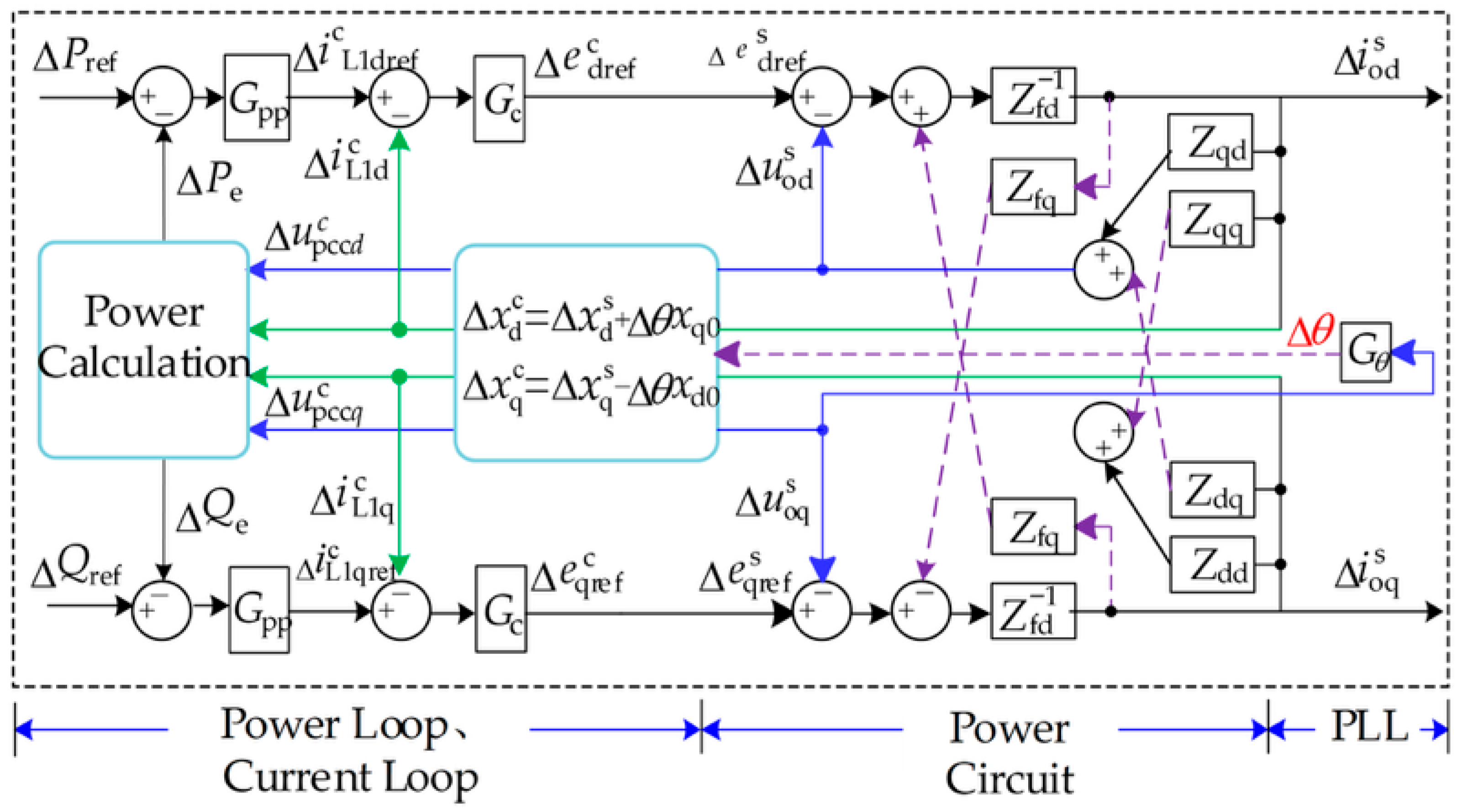
Figure 10 depicts the small signal model structure of the closed-loop system.

3.3. Full-System Modal Impedance Matrix Formulation

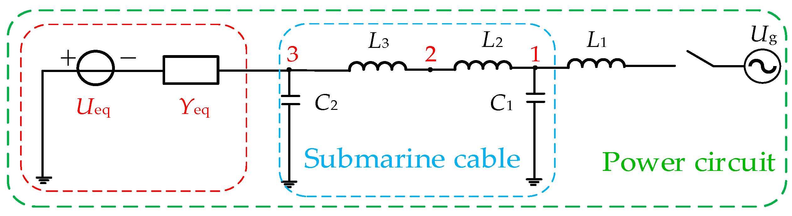
The structure of the direct-drive wind turbine system integrated via a π-type circuit is shown in Figure 11. The network comprises three nodes. By representing the wind turbine admittance as an equivalent Y_eq (obtained from Section 3.1), the corresponding equivalent circuit diagram is illustrated in Figure 11.

The node admittance matrix Y_n for the full system is obtained as:

$$\begin{array}{l}{\mathit{Y}}_n=\left[\begin{array}{ccc}{\mathit{Y}}_{\mathbf{11}}& {\mathit{Y}}_{\mathbf{12}}& {\mathit{Y}}_{\mathbf{13}}\\ {\mathit{Y}}_{\mathbf{21}}& {\mathit{Y}}_{\mathbf{22}}& {\mathit{Y}}_{\mathbf{23}}\\ {\mathit{Y}}_{\mathbf{31}}& {\mathit{Y}}_{\mathbf{32}}& {\mathit{Y}}_{\mathbf{33}}\end{array}\right]\\ =\left[\begin{array}{ccc}{\mathit{Y}}_{\mathit{L}\mathbf{1}}+{\mathit{Y}}_{\mathit{L}2}+{\mathit{Y}}_{\mathit{C}1}& -{\mathit{Y}}_{\mathit{L}2}& 0\\ -{\mathit{Y}}_{\mathit{L}2}& {\mathit{Y}}_{\mathit{L}2}+{\mathit{Y}}_{\mathit{L}3}& -{\mathit{Y}}_{\mathit{L}3}\\ 0& -{\mathit{Y}}_{\mathit{L}3}& {\mathit{Y}}_{\mathit{L}3}+{\mathit{Y}}_{\mathit{C}2}+{\mathit{Y}}_{\mathit{e}\mathit{q}}\end{array}\right]\end{array}$$

(33)

where:

$$\begin{array}{l}{\mathit{Y}}_{\mathit{L}\mathit{n}\mathit{d}\mathit{q}}={\mathit{Z}}_{\mathit{L}\mathit{n}\mathit{d}\mathit{q}}^{-1}\\ {\mathit{Y}}_{\mathit{C}\mathit{n}\mathit{d}\mathit{q}}={{\mathit{Z}}_{\mathit{C}\mathit{n}\mathit{d}\mathit{q}}}^{-1}\\ {\mathit{Z}}_{\mathit{L}\mathit{n}\mathit{d}\mathit{q}}=\left[\begin{array}{cc}{R}_n+s\ast L_n& -\omega \ast L_n\\ \omega \ast L_n& R_n+s\ast L_n\end{array}\right]\\ Z_{\mathit{C}\mathit{n}\mathit{d}\mathit{q}}=\left[\begin{array}{cc}{R}_n+s\ast C_n& -\omega \ast L_n\\ \omega \ast L_n& R_n+s\ast C_n\end{array}\right]\\ {\mathit{Y}}_{\mathit{e}\mathit{q}}=\left[\begin{array}{cc}{Y}_{\mathrm{dd}}& Y_{\mathrm{dq}}\\ Y_{\mathrm{qd}}& Y_{\mathrm{qq}}\end{array}\right]\end{array}$$

(34)

4. Harmonic Resonance Analysis and Mitigation for Offshore Wind Power Systems in dq-Domain

4.1. dq-Domain-Based Modal Analysis of Harmonic Resonance for Offshore Wind Power Systems

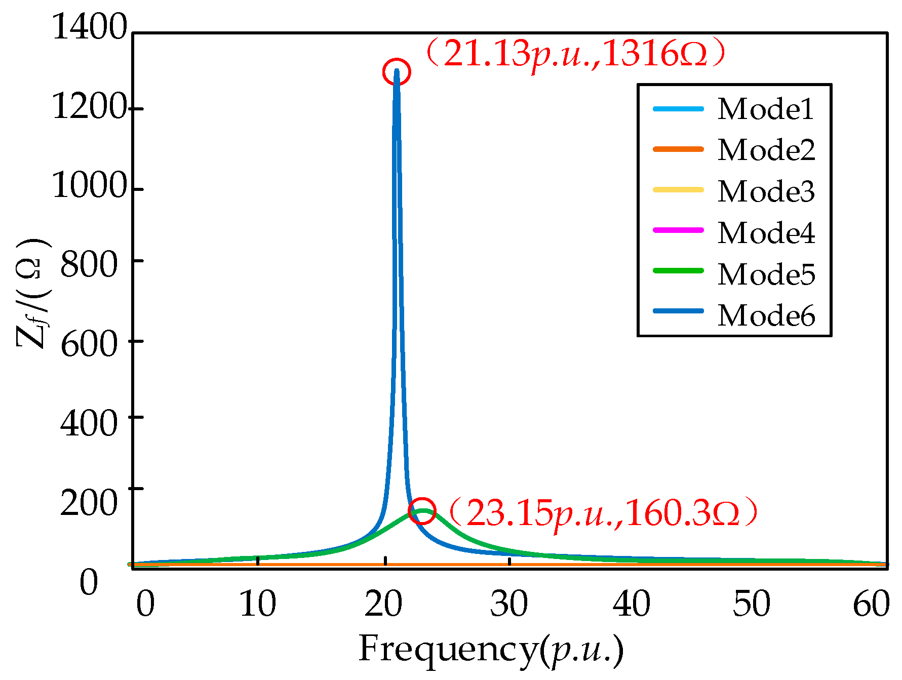
The essential electrical and control parameters of the system are presented in

Table 2. Main Electrical and Control Parameters of the System.

Parameter	Value
Inductance Lg/mH	0.063
Inductance L1/mH	0.849
Inductance L2/mH	0.849
Resistance R1/Ω	0.04
Resistance R2/Ω	0.835
Resistance R3/Ω	0.835
Capacitance C1/mF	0.01
Capacitance C2/mF	0.01
Active Power Loop Proportional Gain KPP	0.002
Active Power Loop Integral Gain KPI	0.01
Reactive Power Loop Proportional Gain KQP	0.002
Reactive Power Loop Integral Gain KQI	0.01
PLL Proportional Gain Kppll	1.84
PLL Integral Gain Kipll	525.92

. By performing eigenvalue decomposition on the node admittance matrix derived in the previous section, the modal analysis impedance curves are obtained, as shown in Figure 12. According to the figure, two resonance points appeared at 21.13 p.u. and 23.15 p.u. which were approximately symmetric about 22.14 p.u.

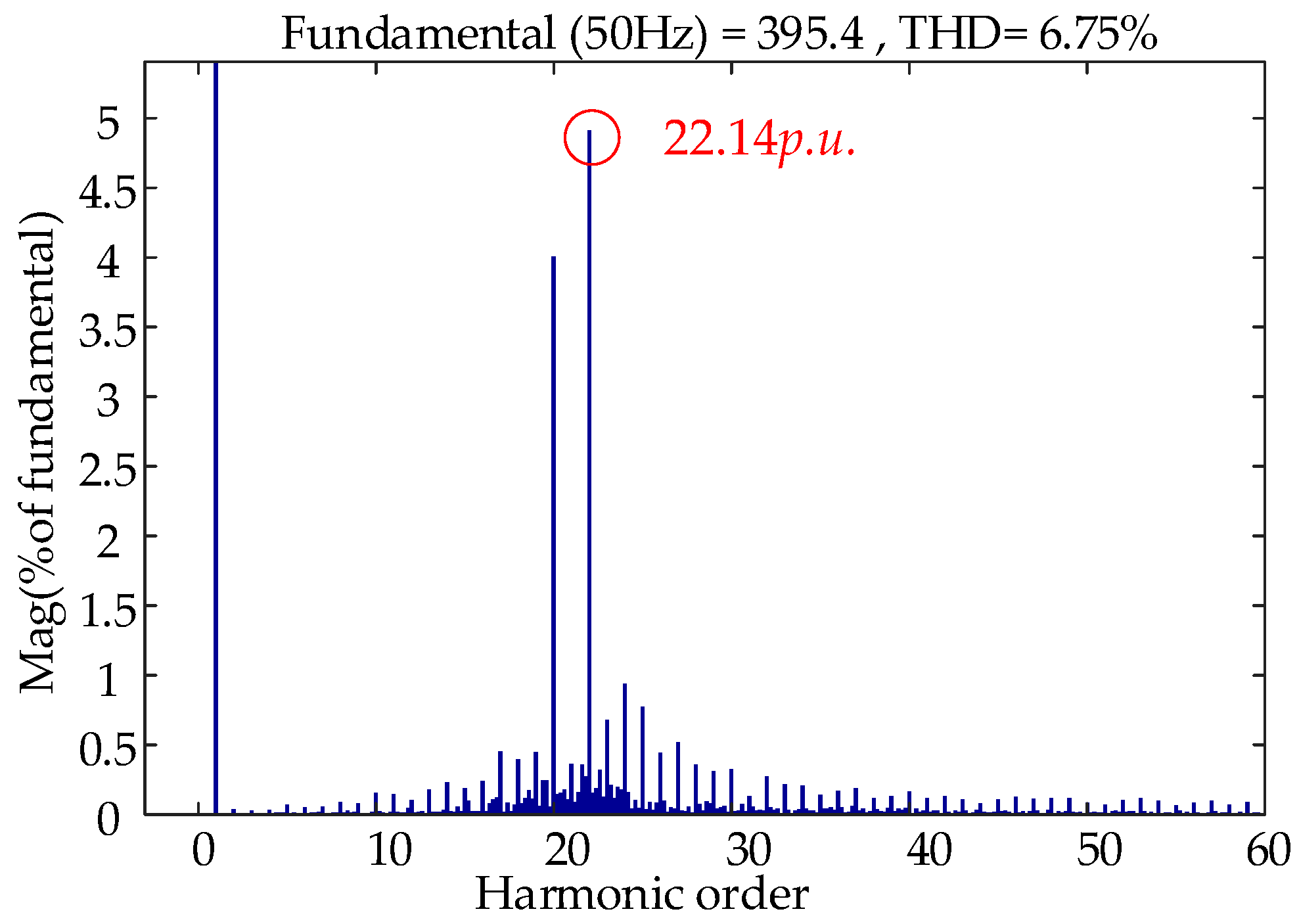
A direct-drive wind turbine model was established in Simulink, and FFT analysis was performed on the node voltages, yielding the results shown in Figure 13. The figure exhibited a resonance at 22.14 p.u. which is consistent with the aforementioned modal analysis results. Therefore, the modal analysis of the direct-drive wind turbine is validated.

The modal analysis indicators are listed in

Table 3. Modal Analysis Indicators for Direct-Drive Wind Turbine π-Type Systems.

Resonance Frequency/p.u.		23.15 (Mode 5)	21.13 (Mode 6)
Critical eigenvalue		0.0178∠5.35°	0.0008∠−169.78°
Key left eigenvectors	Mode1	L5-1 = 0.0346∠7.29°	L6-1 = 0.0082∠−137.41°
	Mode 2	L5-2 = 0.0075∠−141.76°	L6-2 = 0.0342∠5.69°
	Mode 3	L5-3 = 0.4811∠4.44°	L6-3 = 0.1138∠−140.33°
	Mode 4	L5-4 = 0.1052∠−144.02°	L6-4 = 0.4799∠3.10°
	Mode 5	L5-5 = 0.9276∠ 0.99°	L6-5 = 0.2193∠−140.30°
	Mode 6	L5-6 = 0.2008∠−147.22°	L6-6 = 0.9256∠3.14°
Participation factors (magnitude)	Node1	PF51 = 0.0011	PF61 = 0.0011
	Node2	PF52 = 0.2119	PF62 = 0.2117
	Node3	PF53 = 0.7870	PF63 = 0.7873

. Specifically, the two critical resonance frequencies, 21.13 p.u. and 23.15 p.u. corresponded to Mode 5 and Mode 6, respectively. As can be seen from Table 3, the system resonances were primarily caused by Node 3 (79%) and Node 2 (21%), while the influence of Node 1 was negligible.

4.2. Impact of Various Control Parameters on Harmonic Resonance in Offshore Wind Power Systems and Mitigation Methods

In order to explore the specific effects of controller parameters on harmonic resonance, this section takes the power control loop of a direct-drive wind turbine as the research object. The influence of the integral gain K_PI and proportional gain K_PP on the resonance characteristics of the π-type line system was analyzed.

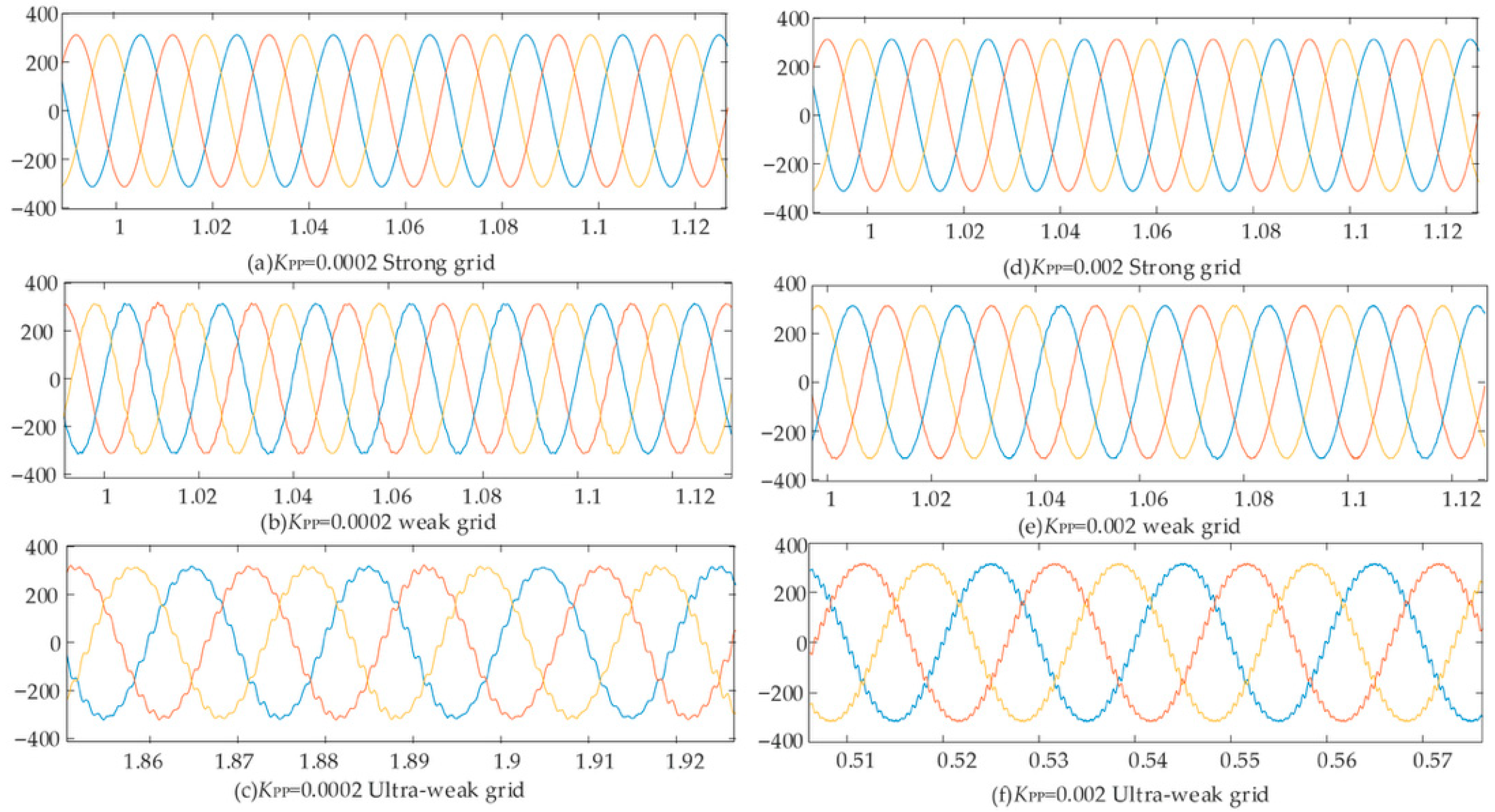
This study was conducted under the premise that the system is stable. Prior to performing modal analysis, a stability analysis must be carried out to ensure that the system is stable. Therefore, both before and after the change in K_PP, the system remains stable under different grid strengths, as shown in Figure 14.

The three-phase voltage waveforms for the system with K_PP = 0.0002 and K_PP = 0.002 under different grid strengths are listed below. As can be seen from the figures, although the increase in K_PP changed the damping characteristics of the resonant modes, the three-phase voltage waveforms of the system remained stable within the selected range. This proves that within the parameter range discussed in this paper, improving resonant damping does not come at the expense of overall stability.

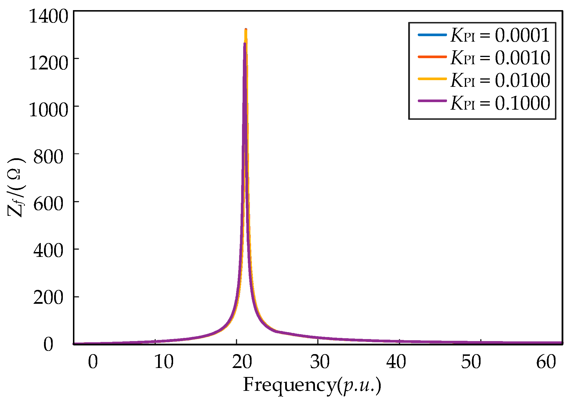
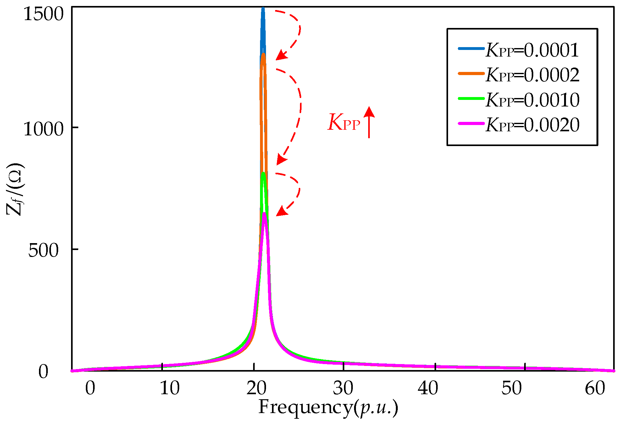
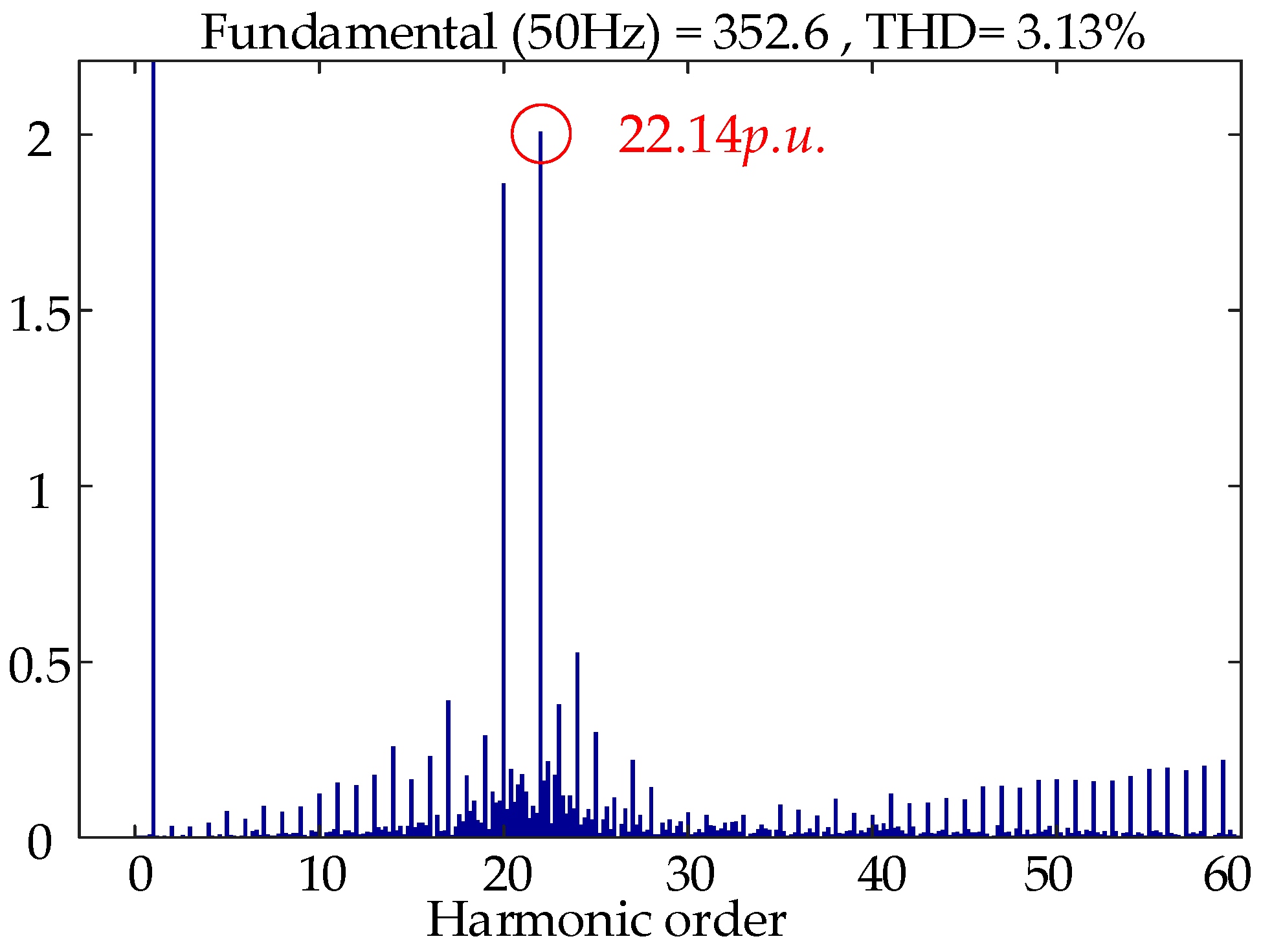
Through modal analysis, the maximum modal impedance curves of the system were obtained for varying K_PI (at constant K_PP) and varying K_PP (at constant K_PI), as depicted in Figure 15 and Figure 16, respectively. The FFT analysis results for K_PP = 0.002 are shown in Figure 17. Combining the data from Figure 12, Figure 13, Figure 14, Figure 15 and Figure 16, it can be observed that:

• Resonant Frequency: Regardless of the value of K_PP, a very sharp resonant peak consistently exists at a frequency of approximately 22.14 p.u. (corresponding to 1107 Hz with a base frequency of 50 Hz). This indicates that the resonance mode is dominated by the physical structure of the system, and the control parameters primarily influence the severity of the resonance rather than its frequency location.
• K_PI: As illustrated in Figure 15, when the power loop integral parameter K_PI varies across a wide range from 0.0001 to 0.1000, the maximum modal impedance curves of the system almost entirely overlap. The resonance frequency remains locked at approximately 22.14 p.u. and the peak amplitude is maintained at around 1350 Ω without any significant upward or downward trend. These results suggest that the system’s high-frequency resonant behavior remains largely unaffected by changes in the power loop integral gain.
• K_PP: As the power loop proportional gain K_PP increases, the magnitude of the resonant peak is significantly suppressed. When K_PP was at its minimum, the resonant peak reached its highest value of nearly 1500 Ω, indicating intense resonance at this frequency. As K_PP gradually increased, the peak height decreased sequentially. When K_PP reached 0.0020, the resonant peak was suppressed to below 700 Ω, resulting in a marked improvement in system resonance. Specifically, when K_PP = 0.0001, the high impedance at the resonant point triggered a strong harmonic response, leading to a THD as high as 6.46%. When K_PP increased to 0.0020, the THD significantly dropped to 3.13%, demonstrating an enhancement in power quality.

It can be concluded that in this grid-connected direct-drive wind turbine system, the proportional coefficient K_PP of the power control loop is the critical variable for regulating high-frequency impedance characteristics and suppressing harmonic resonance. Conversely, the integral coefficient K_PI primarily influences the steady-state performance of the system and has a negligible impact on resonance suppression under high-frequency modes. Therefore, priority should be given to the damping optimization design of K_PP when performing system stability optimization and parameter management.

Although increasing K_PP effectively enhances the system’s ability to suppress harmonic resonance, its practical value requires a trade-off among multiple performance metrics in engineering applications. First, regarding stability margins, as K_PP increases, the open-loop gain curve shifts upward, which may compress the phase margin and reduce the system’s robustness against large disturbances. Second, concerning transient performance, while an excessively high proportional gain accelerates response speed, insufficient system damping will lead to significant overshoot or slow oscillation decay during power step transitions. Furthermore, an overly large gain amplifies the high-frequency noise captured by sensors, degrading the smoothness of control commands. Therefore, the optimized range of K_PP proposed in this paper aims to ensure that the system balances resonance suppression effectiveness with sufficient stability margins under both strong and weak grid conditions.

Therefore, for the direct-drive wind turbine system investigated in this study, appropriately increasing the power loop proportional gain K_PP is an effective means of suppressing system harmonic resonance.

5. Experimental Verification

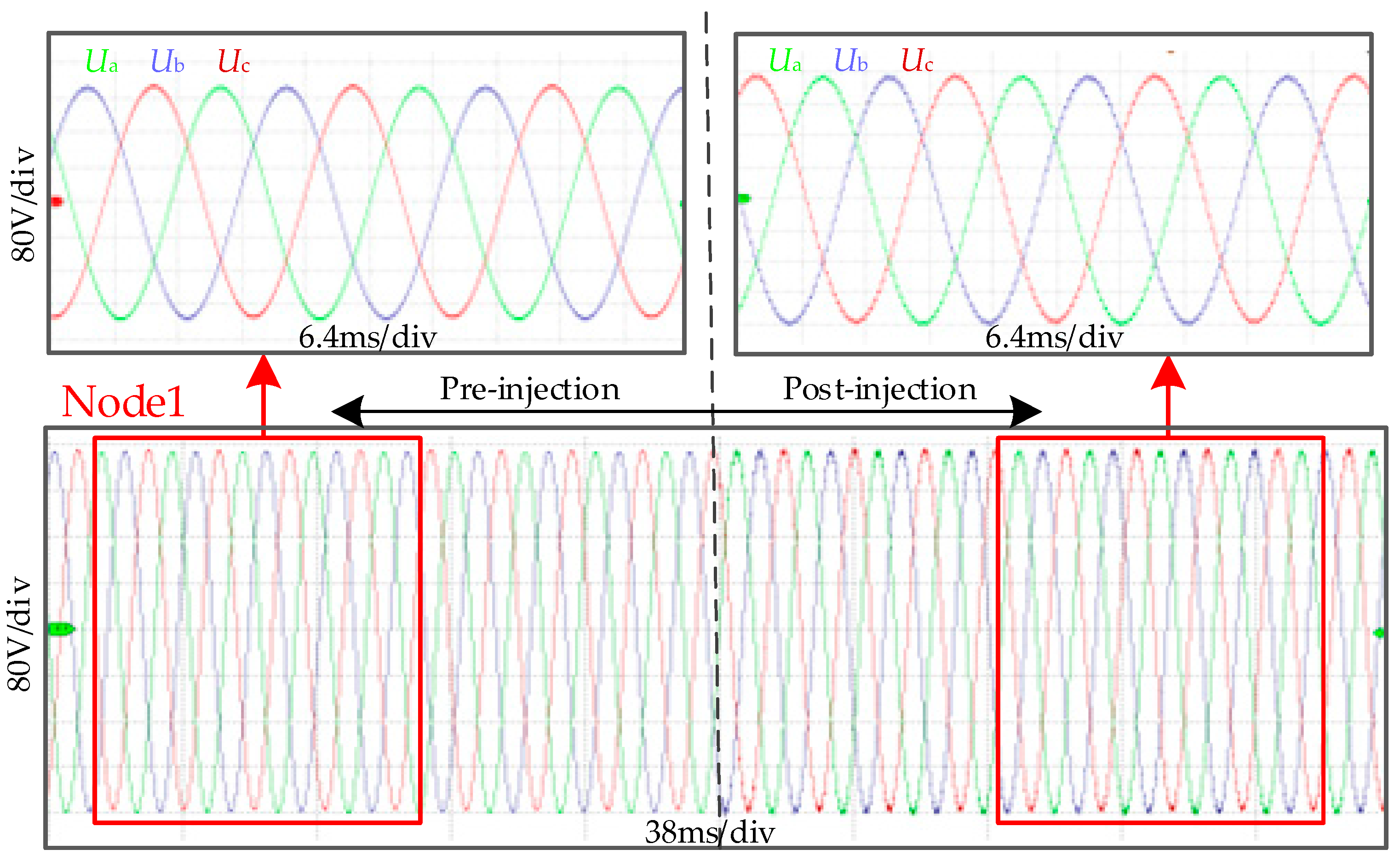
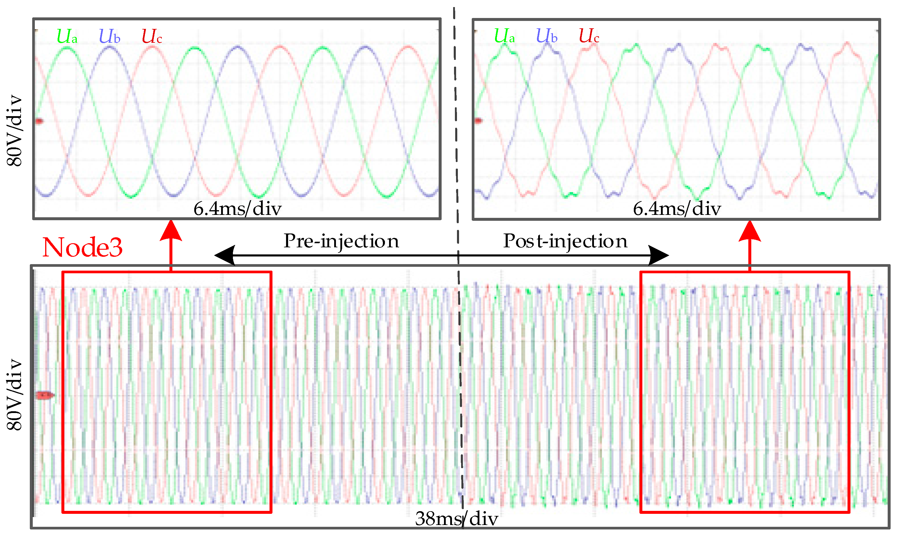
In the previous section, a three-node test system was established to verify the accuracy of the dq-frame modal analysis method. Experimental verification was conducted by injecting disturbance currents at Node 2 with frequencies of 51.6 p.u. and 9.62 p.u., respectively, and an amplitude of 0.01 p.u. The resulting voltage waveforms for Node 1 and Node 3 are shown in Figure 18 and Figure 19, respectively. The following observations can be made.

After injecting a disturbance current with a specific frequency of 51.6 p.u. at Node 2, as illustrated in the enlarged region on the right side of the figure, the voltage waveform at Node 1 also exhibited a distinct response. Finer high-frequency oscillation components were superimposed on the sinusoidal envelope of the voltage at Node 1, leading to a noticeable increase in waveform glitches and a clear resonance characteristic following excitation.

Similarly, when a disturbance current at 9.62 p.u. was injected at Node 2, the voltage waveform at Node 3 underwent substantial changes. Comparing the details before and after the injection, it was found that the post-resonance waveform showed not only a slight increase in amplitude, but also prominent high-frequency oscillations superimposed at the peaks and troughs, presenting typical resonance distortion characteristics.

These distinct oscillations indicate that the frequency of the injected current is highly close to the inherent modal frequency of the system at this operating point, thereby triggering a quasi-resonant state. The experimentally observed voltage distortion phenomena are in full agreement with the resonance characteristics predicted by the dq-frame modal analysis discussed previously. This strongly validates the accuracy of the dq-frame modal analysis method proposed in this paper.

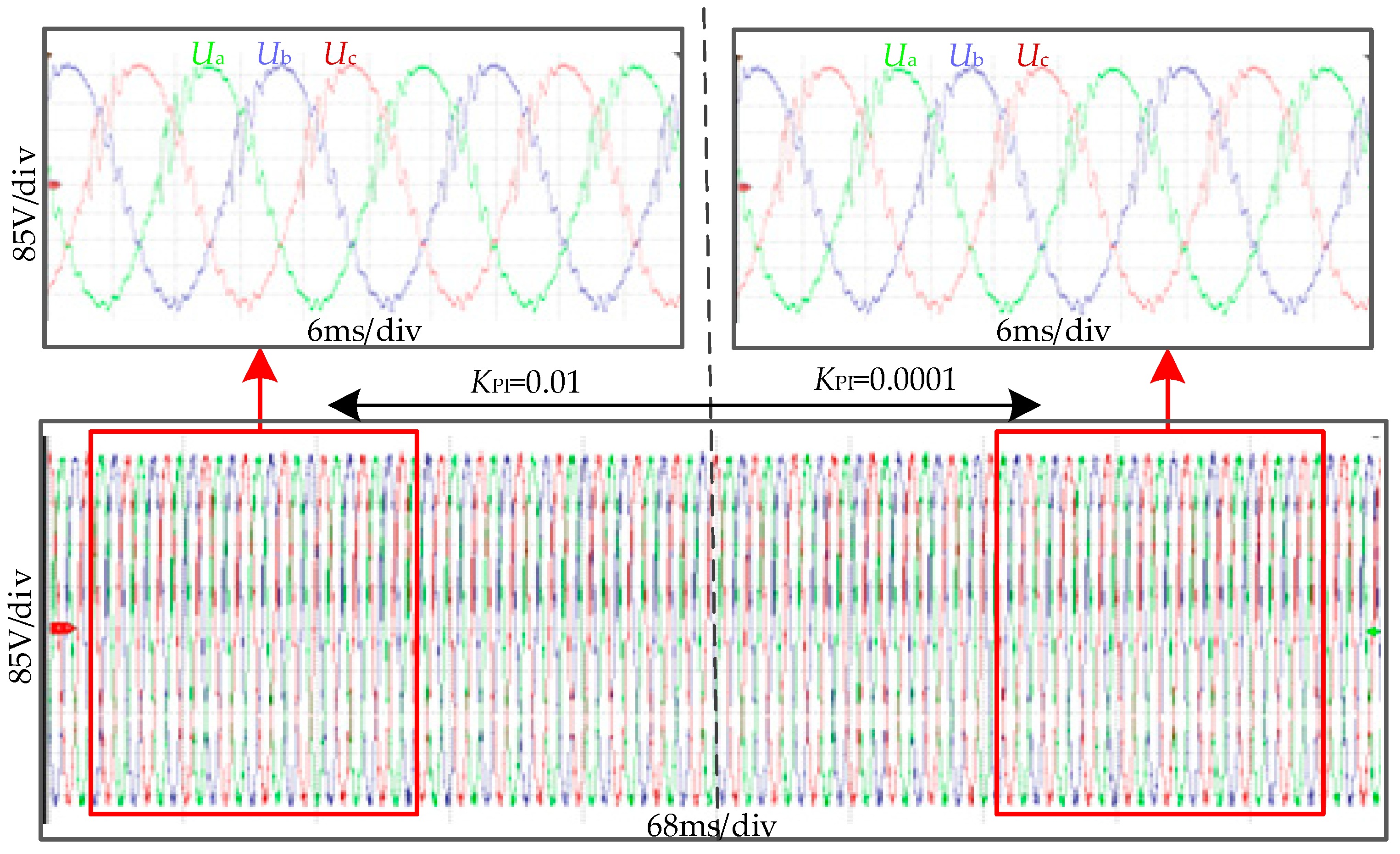
To verify the effects of the power loop control parameters K_PP and K_PI on resonance, experimental validation was conducted on the direct-drive wind turbine system. When the power loop integral parameter K_PI was adjusted, no significant changes were observed in the system voltage waveforms. Whether during the initial operating phase with K_PI = 0.01 or after K_PI was reduced to 0.0001, distinct high-frequency oscillations and distortion components remained superimposed on the three-phase voltage waveforms. As illustrated in Figure 20, the degree of waveform glitches and the resonance characteristics remained essentially consistent.

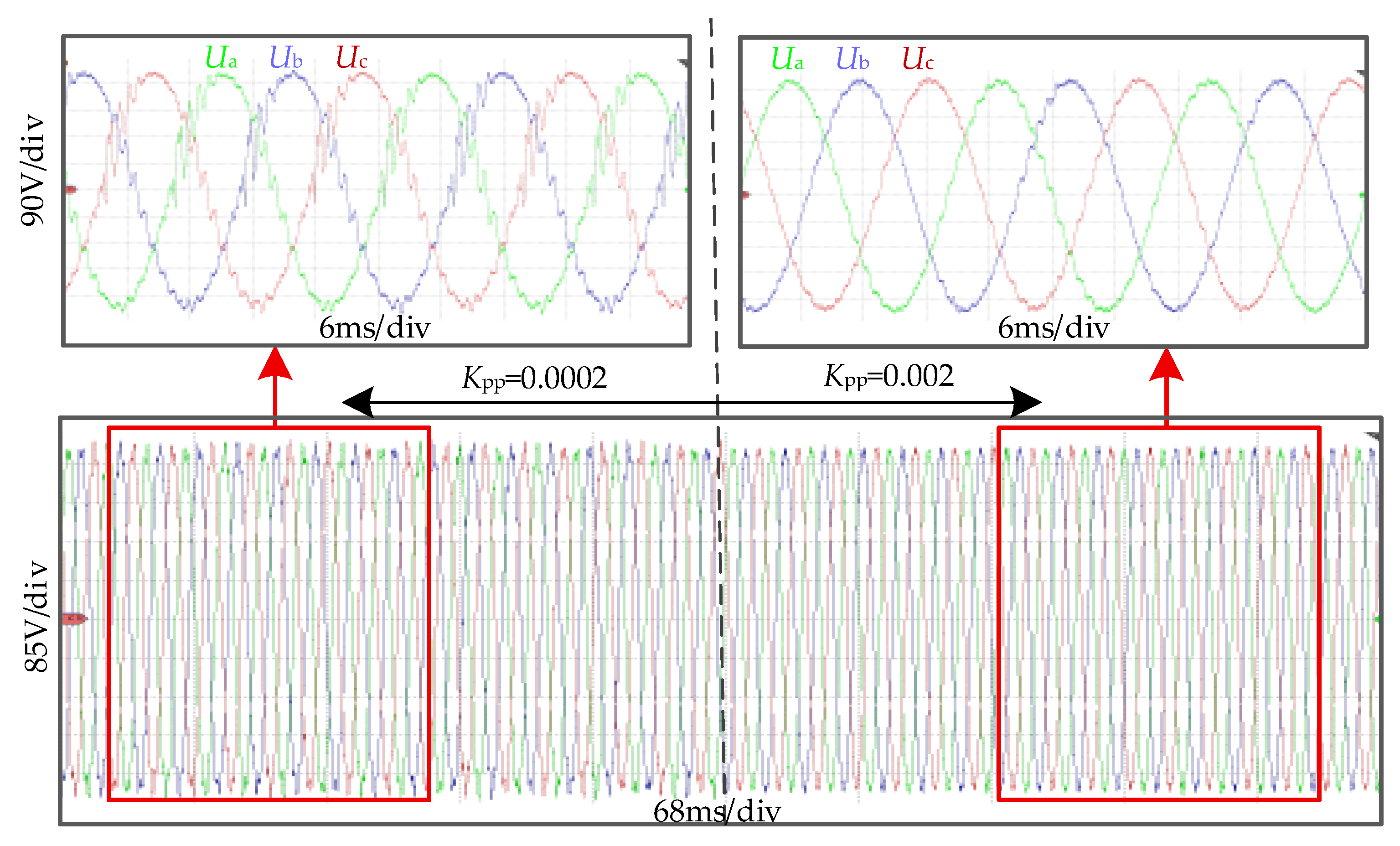
Regarding the adjustment of the power loop proportional parameter K_PP, the value was initially set to 0.0002 and subsequently increased to 0.002 at a specific time to observe the response at the resonant node. As shown in Figure 21, during the initial phase with K_PP = 0.0002 (see the magnified area on the left), the three-phase voltage waveforms at the resonant node exhibited severe quality degradation. The waveform surfaces were heavily superimposed with high-frequency burrs, presenting clear nonlinear distortion and high-frequency oscillation characteristics. This indicates that at low parameter settings, the power loop fails to provide sufficient positive damping for the system at this frequency point, leading to a mismatch between the system impedance characteristics and the grid-side impedance and thus exciting a strong resonant response.

When K_PP was increased to 0.002 via a step change, the system response improved remarkably. The magnified area on the right clearly demonstrates that the previously violent oscillations in the voltage waveform converged rapidly within a very short time, restoring the waveforms to a smooth state with symmetrical amplitudes. The oscillation components at the peaks were effectively eliminated, and the THD of the voltage was significantly reduced.

These comparative experimental results not only provide an intuitive time-domain visualization of the entire process from resonance onset to suppression, but also validate the engineering practical value of the proposed resonance suppression scheme under actual offshore wind power operating conditions.

6. Conclusions

This paper addresses the harmonic resonance issues in offshore wind power systems by proposing and applying a modal analysis method based on the dq rotating reference frame. The accuracy of this method was first validated using a three-node test system. On this basis, this paper established a harmonic resonance analysis model incorporating a direct-drive wind turbine, a π-type equivalent line, and a weak power grid, and conducted an in-depth modal analysis of this model by adopting the proposed method. The resonant frequencies identified by the proposed method exhibited high consistency with the FFT results obtained from Simulink time-domain simulations, thereby confirming the effectiveness of dq-domain modal analysis for the precise evaluation of resonance issues in offshore wind power systems. Several conclusions can be derived as follows:

• The dq-domain modal analysis method effectively uncovered the internal dynamic interaction mechanisms of the system. Through the calculation of the system’s eigenvalues, this method enables the accurate prediction of potential resonant frequencies as well as the quantification of each node’s resonance participation degree. Furthermore, by analyzing the participation factors of state variables associated with each mode, the key factors triggering resonance can be clearly identified. This elucidates the complex coupling paths between different inverters, control loops, and grid impedances, providing a robust theoretical foundation for understanding resonance mechanisms and formulating targeted mitigation strategies.
• Through parameter scanning using the modal analysis method, this study demonstrated that the proportional gain of the power control loop (K_PP) has a significant impact on the system’s resonance modes. Increasing this gain is equivalent to injecting positive active damping into the system, which significantly suppresses resonant peaks, mitigates harmonic amplification, and reduces the THD. Effectively adjusting controller parameters via modal analysis serves as an active, flexible, and economical means of resonance suppression, providing critical technical support for harmonic resonance mitigation in offshore wind farms.

References

1. Ullah, T.; Sobczak, K.; Li´skiewicz, G.; Khan, A. Two-Dimensional URANS Numerical Investigation of Critical Parameters on a Pitch Oscillating VAWT Airfoil under Dynamic Stall. Energies 2022, 15, 5625. [Google Scholar] [CrossRef]
2. Williams, R.; Zhao, F. Global Offshore Wind Report 2024; Global Wind Energy Council: Brussels, Belgium, 2024. [Google Scholar]
3. Dai, L.; Wang, H.; Qin, Y.; Shi, G.; Zhang, J.; Cai, X. Analysis and Suppression of High-Frequency Resonance for Offshore Wind Power Grid-Connected Converter Considering Cable Capacitance Effect. Electronics 2023, 12, 2638. [Google Scholar] [CrossRef]
4. Lee, K.; Yoon, M.; Lee, J.; Gham, S.; Choi, S. Impact of Short Circuit Ratio on Harmonic Distortion in Offshore Wind Farm Integration. Energies 2025, 18, 5480. [Google Scholar] [CrossRef]
5. Yang, B.; Liu, B.; Zhou, H.; Wang, J.; Yao, W.; Wu, S.; Shu, H.; Ren, Y. A critical survey of technologies of large offshore wind farm integration: Summary, advances, and perspectives. Prot. Control Mod. Power Syst. 2022, 7, 233–264. [Google Scholar] [CrossRef]
6. Wang, X.; Blaabjerg, F.; Wu, W. Modeling and analysis of harmonic stability in an AC power-electronics based power system. IEEE Trans. Power Electron. 2014, 29, 6421–6432. [Google Scholar] [CrossRef]
7. Lokar, J.; Dolenc, J.; Blažič, B.; Herman, L. Harmonic Resonance Identification and Mitigation in Power System Using Modal Analysis. Energies 2021, 14, 4017. [Google Scholar] [CrossRef]
8. Zhang, M.; Wang, J.; Zhang, S.; Gao, L.; Guo, X.; Chen, L.; Xu, Y. Harmonic Resonance Analysis and Impedance Remodeling Method of Multi-Inverter Grid-Connected System. Electronics 2023, 12, 3684. [Google Scholar] [CrossRef]
9. Lyu, J.; Cai, X.; Molinas, M. Frequency domain stability analysis of MMC-based HVdc for wind farm integration. IEEE J. Emerg. Sel. Top. Power Electron. 2015, 4, 141–151. [Google Scholar] [CrossRef]
10. Liu, Q.; Wu, M.; Li, J.; Yang, S. Frequency-scanning harmonic generator for (inter) harmonic impedance tests and its implementation in actual 2× 25 kV railway systems. IEEE Trans. Ind. Electron. 2020, 68, 4801–4811. [Google Scholar] [CrossRef]
11. Huan, C.X.; Tayjasanant, T. Modeling wind power plants in harmonic resonance study-A case study in Thailand. In Proceedings of the International Conference on Information Technology and Electrical Engineering (ICITEE), Yogyakarta, Indonesia, 7–8 October 2013; IEEE: Piscataway, NJ, USA, 2013; pp. 385–390. [Google Scholar]
12. Xu, W.; Huang, Z.; Cui, Y. Harmonic resonance mode analysis. IEEE Trans. Power Deliv. 2005, 20, 1182–1190. [Google Scholar] [CrossRef]
13. Huang, Z.; Cui, Y.; Xu, W. Application of modal sensitivity for power system harmonic resonance analysis. IEEE Trans. Power Syst. 2007, 22, 222–231. [Google Scholar] [CrossRef]
14. Hong, L.; Shu, W.; Wang, J. Harmonic resonance investigation of a multi-inverter grid-connected system using resonance modal analysis. IEEE Trans. Power Deliv. 2018, 34, 63–72. [Google Scholar] [CrossRef]
15. Hu, H.; Tao, H.; Blaabjerg, F. Train–network interactions and stability evaluation in high-speed railways–Part I: Phenomena and modeling. IEEE Trans. Power Electron. 2017, 33, 4627–4642. [Google Scholar] [CrossRef]
16. Liu, Z.; Rong, J.; Zhao, G. Harmonic assessment for wind parks based on sensitivity analysis. IEEE Trans. Sustain. Energy 2017, 8, 1373–1382. [Google Scholar] [CrossRef]
17. Luo, J.; Tong, N.; Bu, S. Internal modal resonance analysis for full converter-based wind generation using analytical inertia model. IEEE Trans. Power Syst. 2023, 39, 3509–3522. [Google Scholar] [CrossRef]
18. Yang, L.; Xu, Z.; Feng, L. Analysis on harmonic resonance of offshore wind farm transmitted by MMC-HVDC system. In Proceedings of the IEEE Innovative Smart Grid Technologies-Asia (ISGT Asia), Chengdu, China, 21–24 May 2019; IEEE: Piscataway, NJ, USA, 2019; pp. 2296–2301. [Google Scholar]
19. Cheah-Mane, M.; Liang, J.; Jenkins, N. Electrical resonance instability study in HVDC-connected offshore wind power plants. In Proceedings of the IEEE Power and Energy Society General Meeting (PESGM), Boston, MA, USA, 17–21 July 2016; IEEE: Piscataway, NJ, USA, 2016; pp. 1–5. [Google Scholar]
20. Sowa, I.; Domínguez-García, J.L.; Gomis-Bellmunt, O. Impedance-based analysis of harmonic resonances in HVDC connected offshore wind power plants. Electr. Power Syst. Res. 2019, 166, 61–72. [Google Scholar] [CrossRef]
21. Xin, Y.L.; Tang, W.H.; Luan, L.; Chen, G.Y.; Wu, H. Overvoltage protection on high-frequency switching transients in large offshore wind farms. In Proceedings of the IEEE Power and Energy Society General Meeting (PESGM), Boston, MA, USA, 17–21 July 2016; IEEE: Piscataway, NJ, USA, 2016; pp. 1–5. [Google Scholar]
22. Sainz, L.; Monjo, L.; Pedra, J.; Cheah-Mane, M.; Liang, J.; Gomis-Bellmunt, O. Effect of wind turbine converter control on wind power plant harmonic response and resonances. IET Electr. Power Appl. 2017, 11, 157–168. [Google Scholar] [CrossRef]
23. Wang, L.; Xie, X.; Jiang, Q.; Pota, H.R. Mitigation of multimodal subsynchronous resonance via controlled injection of supersynchronous and subsynchronous currents. IEEE Trans. Power Syst. 2013, 29, 1335–1344. [Google Scholar] [CrossRef]
24. Liserre, M.; Blaabjerg, F.; Hansen, S. Design and control of an LCL-filter-based three-phase active rectifier. IEEE Trans. Ind. Appl. 2005, 41, 1281–1291. [Google Scholar] [CrossRef]
Figure 1. Offshore wind power converter system.
Energies 19 00947 g001
Figure 2. Flowchart of modal analysis in the dq frame.
Energies 19 00947 g002
Figure 3. Thévenin equivalent circuit of the three-node test system.
Energies 19 00947 g003
Figure 4. Modal impedance curves of the three-node test system.
Energies 19 00947 g004
Figure 5. Modal impedance curves of the three-bus test system in the dq frame.
Energies 19 00947 g005
Figure 6. Simulink FFT analysis diagram of the 3-bus system in the dq frame.
Energies 19 00947 g006
Figure 7. Configuration of an offshore wind power system with direct-drive wind turbines.
Energies 19 00947 g007
Figure 8. PLL Structure and Linearized Model.
Energies 19 00947 g008
Figure 9. Schematic of the Relationship between Synchronous and Control Reference Frames.
Energies 19 00947 g009
Figure 10. Small signal model structure of the closed-loop system.
Energies 19 00947 g010
Figure 11. Equivalent circuit diagram of a direct-drive wind turbine with a π-type circuit.
Energies 19 00947 g011
Figure 12. Modal impedance diagram of a direct-drive wind turbine with a π-type line.
Energies 19 00947 g012
Figure 13. FFT analysis results of the direct-drive wind turbine π-type line.
Energies 19 00947 g013
Figure 14. Three-phase voltage waveforms of the system under different grid strengths when KPP = 0.0002 and KPP = 0.002.
Energies 19 00947 g014
Figure 15. Maximum modal impedance plot of the direct-drive wind turbine π-type system under varying KPI (at constant KPP).
Energies 19 00947 g015
Figure 16. Maximum modal impedance plot of the direct-drive wind turbine π-type system under varying KPP (at constant KPI).
Energies 19 00947 g016
Figure 17. FFT analysis results with KPP = 0.0020 (at constant KPI).
Energies 19 00947 g017
Figure 18. Voltage waveform response of Node 1 to 51.6 p.u. disturbance.
Energies 19 00947 g018
Figure 19. Voltage waveform response of Node 3 to 9.6 p.u. disturbance.
Energies 19 00947 g019
Figure 20. Voltage waveforms at the resonant point of the direct-drive wind turbine system during changes in KPI.
Energies 19 00947 g020
Figure 21. Voltage waveforms at the resonant point of the direct-drive wind turbine system during changes in KPP.
Energies 19 00947 g021