A Novel Diagnostic Method on the Industrial Boilers Using Machine Learning: t-SNE, Auto-Encoder and LGBM

Abstract

This study presents a machine learning (ML)-based diagnostic framework for industrial boilers, focusing on the reliable classification of normal and abnormal operating states. Experimental data were obtained from a 5-ton field demonstration boiler, including 28,943 samples collected under steady-state and load-swing conditions as well as three abnormal scenarios: fan inverter malfunction, air damper malfunction, and fuel gas damper malfunction. Data preprocessing was performed to normalize and structure multivariate signals, including pressure, temperature, water level, and oxygen concentration for ML implementation. Exploratory data analysis (EDA) and principal component analysis (PCA) were employed to examine distributional characteristics, while t-distributed stochastic neighbor embedding (t-SNE) and autoencoders were applied to enhance visualization and feature extraction. The Light gradient boosting machine (LGBM) served as the primary classification algorithm. Results demonstrate that PCA and t-SNE provided partial separation between normal and abnormal data, but overlapping distributions limited clear boundary identification. Autoencoders improved clustering, showing more distinct separability between operating states. Using LGBM, the model achieved the lowest classification adequacy of 99.64%. This work demonstrates the feasibility of ML-based diagnostics for industrial boilers and underscores the potential of ensemble models such as LGBM for high-accuracy abnormality detection. Future research will expand on this foundation, ultimately supporting the development of commercial-level diagnostic systems.

1. Introduction

In recent years, machine learning (ML)-based diagnostic methods have been increasingly applied across diverse engineering fields, including power generation, heating, defense, and aviation [1,2,3,4,5,6,7]. Among these, the heating sector has attracted particular interest because of its close connection to both industrial performance and public safety. Boilers, which remain one of the most widely used sources of thermal energy for residential and industrial applications, stand at the center of this discussion [8,9]. Boilers are increasingly required to deliver efficiency, scalability, and fuel flexibility; however, these features also expose them to significant operational challenges.

Because boilers must operate continuously under high-temperature and high-pressure conditions, maintaining their stability is essential for ensuring both system reliability and public safety. The urgency of advanced fault diagnosis is underscored by recent statistics; according to the National Fire Data System of South Korea, 815 boiler-related fires occurred between 2021 and 2023, resulting in 36 casualties and property damage exceeding 11.6 billion KRW. The severity is even more pronounced in industrial settings, as seen in a 2021 industrial boiler explosion in South Korea caused by a pressure vessel rupture, which led to fatalities and facility destruction. Beyond safety, from an energy engineering perspective, even minor malfunctions can decrease thermal efficiency by 1–5%, leading to significant annual fuel waste and increased carbon emissions. Thus, developing a highly accurate ML-based diagnostic framework is a critical necessity for both operational safety and sustainable energy management.

The risks are further heightened because large- and medium-scale boilers are frequently situated near residential, commercial, and public facilities, where operational failures can result in severe consequences [10,11]. Without timely and accurate diagnostics, minor irregularities may escalate into equipment damage, extended downtime, or hazardous events such as fires, explosions, or toxic gas leakage [12]. Typical failure modes include nozzle erosion, material fatigue, water-level imbalance, and combustion instability. The potential scale of these accidents highlights the urgent demand for diagnostic systems that are both rapid and reliable in detecting early signs of abnormal operation. By preventing minor anomalies from progressing into critical incidents, such systems not only reduce human and economic losses but also ensure continuous and efficient energy supply.

Several diagnostic methods have been developed and applied to monitor the condition of boilers and to detect potential hazards [13,14,15]. Conventional diagnostic systems typically rely on indicators such as pressure, temperature, water level, oxygen concentration, and vibration, which are measured in real time to determine the operational state of the equipment [16,17,18]. While such approaches remain valuable in modern boiler systems, their limitations have become increasingly apparent due to environmental changes, etc. The currently used method, threshold-based monitoring, often struggles to distinguish between normal fluctuations and genuine precursors of instability, leading to both false alarms and undetected failures. Furthermore, conventional approaches are usually based on single-variable monitoring, which makes it difficult to capture the complex interactions among pressure, temperature, and vibration that characterize abnormal boiler behavior. For example, sensor noise, durability issues, and calibration complexity further constrain the accuracy and applicability of these methods.

To overcome these challenges, artificial intelligence (AI)-based diagnostic methods have attracted growing attention [19,20,21,22]. AI enables the automatic classification of normal and abnormal operating conditions. Unlike conventional methods, AI models can recognize nonlinear patterns and temporal correlations across multiple signals, providing a more holistic view of boiler dynamics [23,24,25]. By analyzing pressure, temperature, and vibration data, AI systems can predict early signs of instability that conventional threshold-based methods often miss. Accordingly, AI-driven diagnostics facilitate proactive early warning, thereby mitigating the risk of critical operational failures [26,27].

ML techniques such as principal component analysis (PCA), t-distributed stochastic neighbor embedding (t-SNE), autoencoders, and light gradient boosting machine (LGBM) have been increasingly applied in the predictive maintenance of rotating machinery, including turbines, compressors, and pumps [28,29,30,31,32,33]. These combined AI models can capture both spatial correlations and temporal dynamics in sensor data, which allows for accurate detection of complex fault signatures.

Extending such methods to boiler systems has recently been attempted, with several studies proposing AI-based approaches for detecting abnormal operating conditions using exhaust gas temperature, chamber pressure, and vibration measurements [34]. However, most existing work has been validated only for narrow operating conditions, specific fuel types, or limited load ranges [35]. As a result, generalizable diagnostic frameworks that can adapt to diverse operating scenarios remain insufficient, especially in the context of evolving boiler applications with alternative fuels [36,37,38,39].

This study proposes an AI-based methodology to classify normal and abnormal operating states in boiler systems by integrating multivariate sensor data obtained from load swing tests. The validation was performed across a load range of 20% to 100%, confirming that the model can adapt to varied operating conditions beyond narrowly defined scenarios. In addition to enhancing diagnostic accuracy, the methodology aims to establish a foundation for generalizable AI-based diagnostics that can be applied to a wide range of boiler configurations and operating environments. Ultimately, this study seeks to contribute to the development of safer and more reliable boiler systems, reducing downtime, preventing accidents, and supporting the broader adoption of advanced diagnostic technologies in industrial heating applications.

2. Experimental Methods

In this study, experimental data are obtained from a 5-ton class boiler (Daelim Royal E&P, Kyoungsan, Republic of Korea) manufactured by Company D and specifications are shown in

Table 1. Specifications of the boiler used in this study.

Specification	Value
Steam flow rate	5000 kg/h
Steam design pressure	1.0 MPa
Steam design temperature	183.33 °C
Steam operating pressure	0.8 MPa
Steam operating temperature	174.69 °C
Maximum water volume	9.5 m3
Fuel consumption	342.9 Nm3/h (LNG 10,430 kcal/Nm3 @ 20 °C water feed)
Overall efficiency	94.3%

. The steam flow rate was 5000 kg/h, indicating the boiler’s capacity to supply steam under full-load operation. The design pressure and temperature were set at 1.0 MPa and 183.33 °C, respectively, which represent the maximum values allowed under standard design conditions. In normal operation, the steam pressure and temperature were maintained at 0.8 MPa and 174.69 °C. The maximum water volume of the boiler was 9.5 m³ and fuel consumption was measured as 342.9 Nm³/h, based on liquefied natural gas with a lower heating value of 10,430 kcal/Nm³ at a feedwater temperature of 20 °C. Under these conditions, the overall efficiency of the boiler was evaluated as 94.3%.

The data collection overview is summarized in

Table 2. Overview of normal and abnormal data collection.

Test	Experimental Condition	Load [%]	Sampling Rate	Total Duration	Number of Samples [ea]
Normal test #1	Load-specific data acquisition, 5 loads (20–100%), ~1 h each	20, 40, 60, 80, 100	1–3 s/sample (irregular)	12 h 16 m	13,266
Normal test #2	Load swing continuous adjustment, 5 loads (ascending/descending), ~10 min each	20 → 40 → 60 → 80 → 100 → 80 → 60 → 40 → 20		3 h 46 m	5756
Abnormal criteria test	Under normal conditions for each load condition prior to abnormal test			5 m (for each abnormal test)	1571
Abnormal test #1	Forced draft fan inverter fault, 3 loads (20%, 60%, 100%)	▪ 20%: +10, +20, +30, −10, −20, −30 ▪ 60%: +10, +20, +30, −10, −20, −30 ▪ 100%: +5, +10, −10, −20, −30		5 h 45 m (total duration of abnormal tests #1–3)	2758
Abnormal test #2	Air damper fault, 3 loads (20%, 60%, 100%)	▪ 20%: +20, +40, +60, −20, −40, −60 ▪ 60%: +10, +20, +30, −10, −20, −30 ▪ 100%: +10, +20, +30, −10, −20, −30			2779
Abnormal test #3	Fuel gas damper fault, 3 loads (20%, 60%, 100%)	▪ 20%: +10, +20, +30, −10%, −20%, −30% ▪ 60%: +10, +20, +30, −10, −20, −30 ▪ 100%: +8, +16, +24, −8, −16, −24			2813

. For normal state experiments, data are collected for a total duration of approximately 12 h. The experiment is conducted as follows:

Normal test #1 (NT₁): this test is carried out under five load conditions in 20%, 40%, 60%, 80%, and 100%, with about 1 h of operation at each load. A total of 13,266 samples is acquired from this test.

Normal test #2 (NT₂): a load swing experiment is conducted for approximately 4 h, during which the load was sequentially varied in 20% → 40% → 60% → 80% → 100% → 80% → 60% → 40% → 20%. During the load swing experiment, an additional 5756 samples were generated.

Prior to the abnormal operation experiments, this study performs a baseline run, in which the boiler was operated for 5 min under each of the five load conditions. These 1571 samples are treated as part of the normal dataset for classification purposes.

For abnormal state experiments, data are collected over approximately 6 h across three fault scenarios. An overview of abnormal experiments is as follows:

Abnormal test #1 (AT₁): Fan inverter malfunction—this test is conducted under three representative load conditions in 20%, 60%, and 100%. Each case includes both excessive and insufficient operations, with three levels each in +10%, +20%, +30% and −10%, −20%, −30%. This scenario produces 2758 samples.

Abnormal test #2 (AT₂): Air damper malfunction—this test is conducted under the same three load conditions in 20%, 60%, and 100%. For each, excessive and insufficient operation was introduced at three levels. For example, at 20% load, the variation included +20%, +40%, +60% and −20%, −40%, −60%. A total of 2779 samples is collected.

Abnormal test #3 (AT₃): Fuel gas damper malfunction—Similarly tested at 20%, 60%, and 100% load conditions, with three excessive and three insufficient levels. For instance, at 20% load, the variation included +10%, +20%, +30% and −10%, −20%, −30%. At 100% load, the steps were adjusted to ±8%, ±16%, and ±24%. This experiment measured 2813 samples.

However, the sampling interval varied irregularly between 1 and 3 s per sample. This fluctuation arises because the facility used a conventional industrial boiler’s sensing system rather than dedicated experimental equipment. Although at least one data point is obtained within any 3 s window, the measurement interval was not perfectly constant. Despite the irregular sampling intervals, the acquired data are sufficiently consistent to permit accurate and meaningful analysis of the boiler system behavior. In total, 28,943 samples are collected throughout all experiments, including 20,593 normal samples and 8350 abnormal samples.

The entire data collection campaign was conducted over a period of multiple days to account for potential variations in ambient environmental conditions, temperature, humidity, system-level fluctuations and so on. This multi-day approach was intended to provide a more diverse dataset for training and a more realistic environment for evaluating the model’s robustness.

The specifications of the sensors used for data acquisition are provided in

Table 3. Sensor information used for data collection.

Type	Manufacturer	Model	Installation Location	Measurement Range	Other Specification
Temperature	KYODONG Electrics	PT-100	Boiler shell, boiler front door, economizer inlet, economizer outlet, burner, feedwater inlet, feedwater outlet, exhaust gas recirculation	−85–200 °C	Accuracy: ±0.15 °C
Pressure	SENSYS	M5200	Pressure piping	350 kPa– 100 MPa	Accuracy: ±0.5%
Vibration	MYUNGSUNG A&T	MS- VTXYZ- C-AL-001	Pump motor base plate, side of forced draft fan motor	0.25–1 g	Sensitivity: ±1 mg, Resonance frequencies: 5.5 kHz and 21 kHz.

. In this table, three types of sensors with clear sensor specifications are described. Temperature measurements are carried out using the #PT-100 resistance temperature detector manufactured by KYODONG Electrics (Republic of Korea). This sensor has a measurement range of −85 to 200 °C with an accuracy of ±0.15 °C, and is widely applied in industrial equipment requiring high precision. In this study, RTDs are installed on the boiler shell, front door, burner, and at the feedwater inlet and outlet. Exhaust gas recirculation pressure is measured by mounting a compact low-cost pressure transducer, SENSYS #M5200 on the piping. The #M5200 sensor provides a measurement range of 350 kPa to 100 MPa with an accuracy of ±0.5%. Vibration is monitored using the #MS-VTXYZ-C-AL-001 sensor supplied by MYUNGSUNG A&T. This measuring sensor has a sensitivity of ±1 mg, a measurement range of 0.25–1 g, and resonance frequencies at 5.5 kHz and 21 kHz.

3. Experimental Results and Discussion

3.1. Test Results Under Different Load Conditions

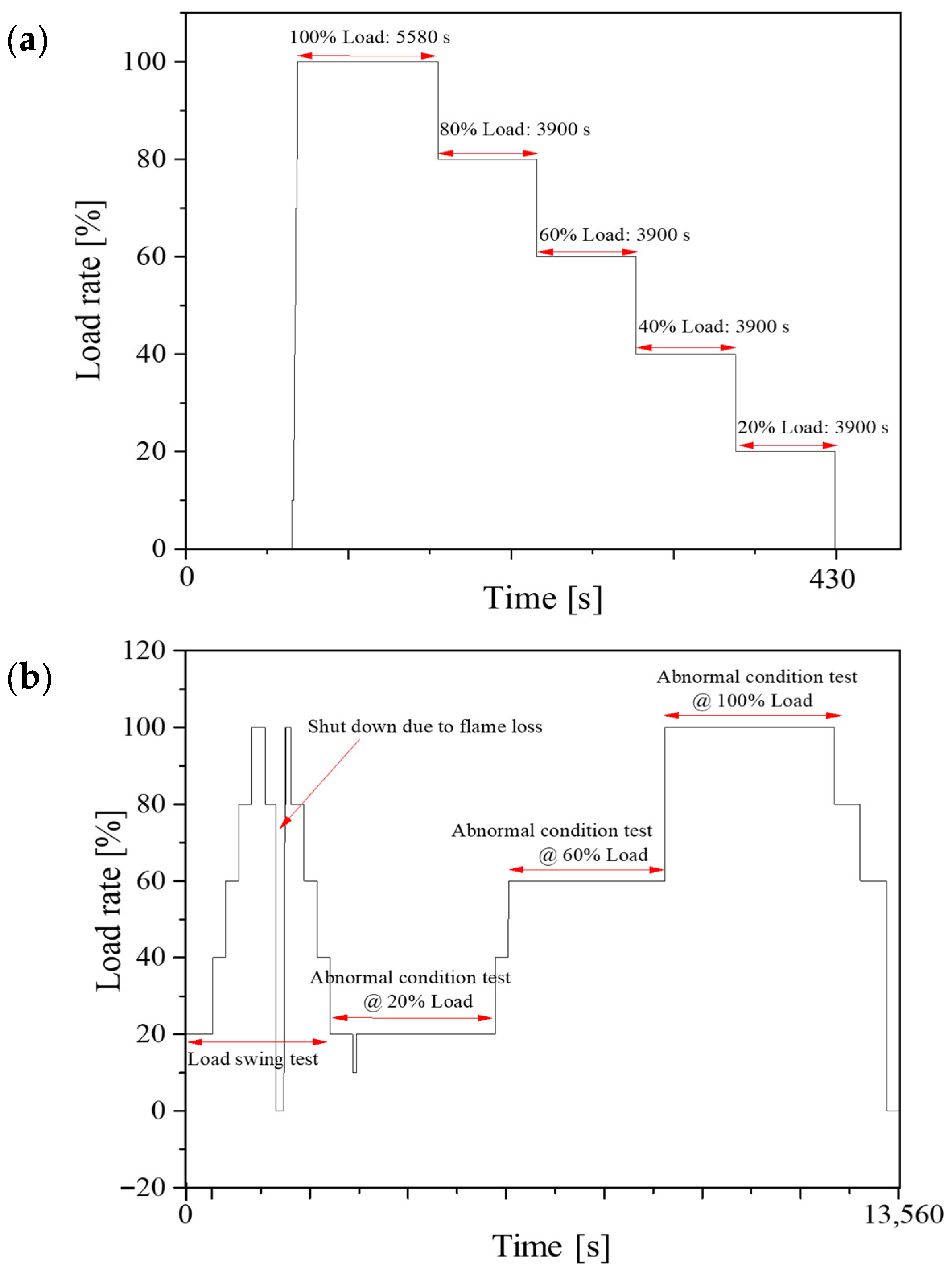
The load information of the normal data collected under each operating condition is illustrated as a time-series graph, as shown in Figure 1a. The graph presents the preparatory data recorded prior to the load tests, followed by the measurement of data for one hour each at 100%, 80%, 60%, 40%, and 20% load conditions.

While the load swing test and abnormal tests were conducted sequentially within a single operational window, the entire experimental campaign spanned across different operating days. This temporal separation allows the dataset to include natural fluctuations in external environmental factors, which are essential for testing the model’s ability to generalize. The load profile over time, shown in Figure 1b, indicates the sequence of experiment. After the load swing test, abnormal data collection is conducted at 20%, 60%, and 100% load conditions. Approximately 10 min of data are measured at each load level. By collecting continuous data across different loads, this test is designed to supplement the static behavior dataset of normal operation with dynamic behavior data.

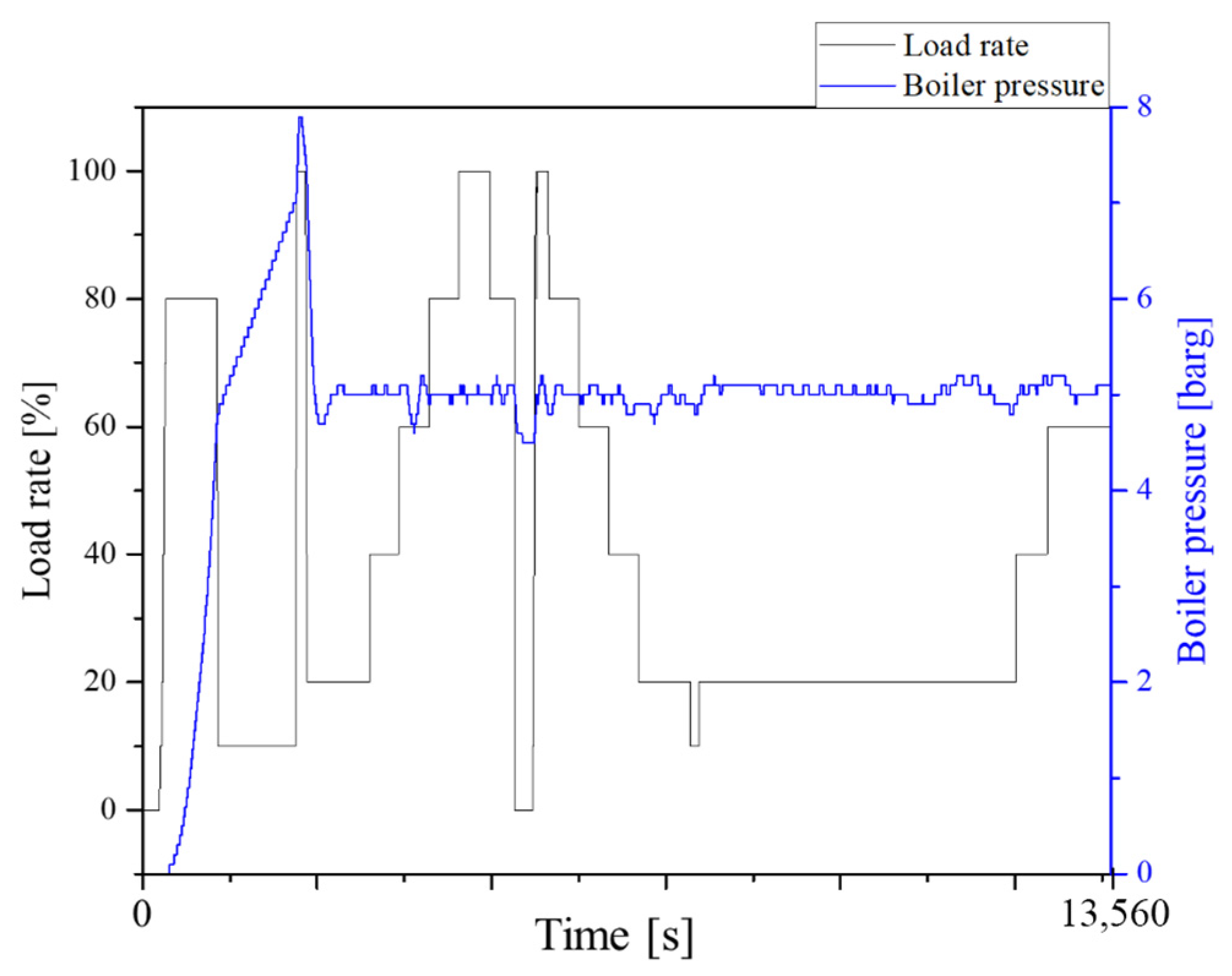
As shown in Figure 1b, which is presented together with the load swing experiment, the procedure and timing of abnormal data acquisition under different load conditions are confirmed. From the abnormal data collected at each load, pressure was selected as a representative signal of the boiler operating state and is illustrated in Figure 2. The graph shows that while pressure generally follows the load, distinct fluctuations and deviations from the steady-state baseline occur during induced malfunctions, confirming its diagnostic relevance. This graph illustrates the variations in load and boiler pressure observed during abnormal data acquisition under different operating conditions. For the development of the ML code, Python version 3.8.5, NumPy version 1.18.1, Pandas version 1.1.5, and Scikit-learn version 0.22.1 are used.

While the experimental data provides a detailed record of the boiler’s behavior, these raw signals are not yet ready for ML. The data comes in various units and was recorded at irregular intervals of 1 to 3 s, making it difficult for models to process directly. Therefore, these raw physical measurements must be cleaned, synchronized, and normalized into a consistent format. The following section describes the preprocessing steps taken to transform this raw data into structured inputs that allow the ML models to accurately recognize diagnostic patterns.

3.2. Preprocessing of Experimental Boiler Data

The experimental data obtained from the tests require preprocessing prior to being introduced into the ML code. The process consists of the following steps: raw data input, data reading, data inspection, data visualization, preprocessing, and data storage, which ultimately convert the dataset into a form suitable for ML implementation. Additionally, for clear analysis, specific intervals representing the boiler load rate and operating state were selected and used for ML analysis, gathering approximately 1870 data samples. The preprocessing process is as follows:

• Raw data input: Experimental measurements of boiler variables, including pressure, temperature, water level, and oxygen concentration, are imported into the preprocessing code.
• Data reading and inspection: The imported data are organized in matrix form, allowing time-series signals to be retrieved within the code. At this stage, units and values are checked to ensure consistency and accuracy.
• Data visualization: Key collected variables are visualized in order to examine load swing conditions and abnormal input scenarios.
• Preprocessing: The raw sensor values are reformatted into floating-point type (float64) for ML processing. Additional tasks such as feature generation and column adjustment are performed to prepare the dataset for modeling.
• Data storage: The processed dataset obtained through steps 1–4 is saved for use in subsequent ML processes.

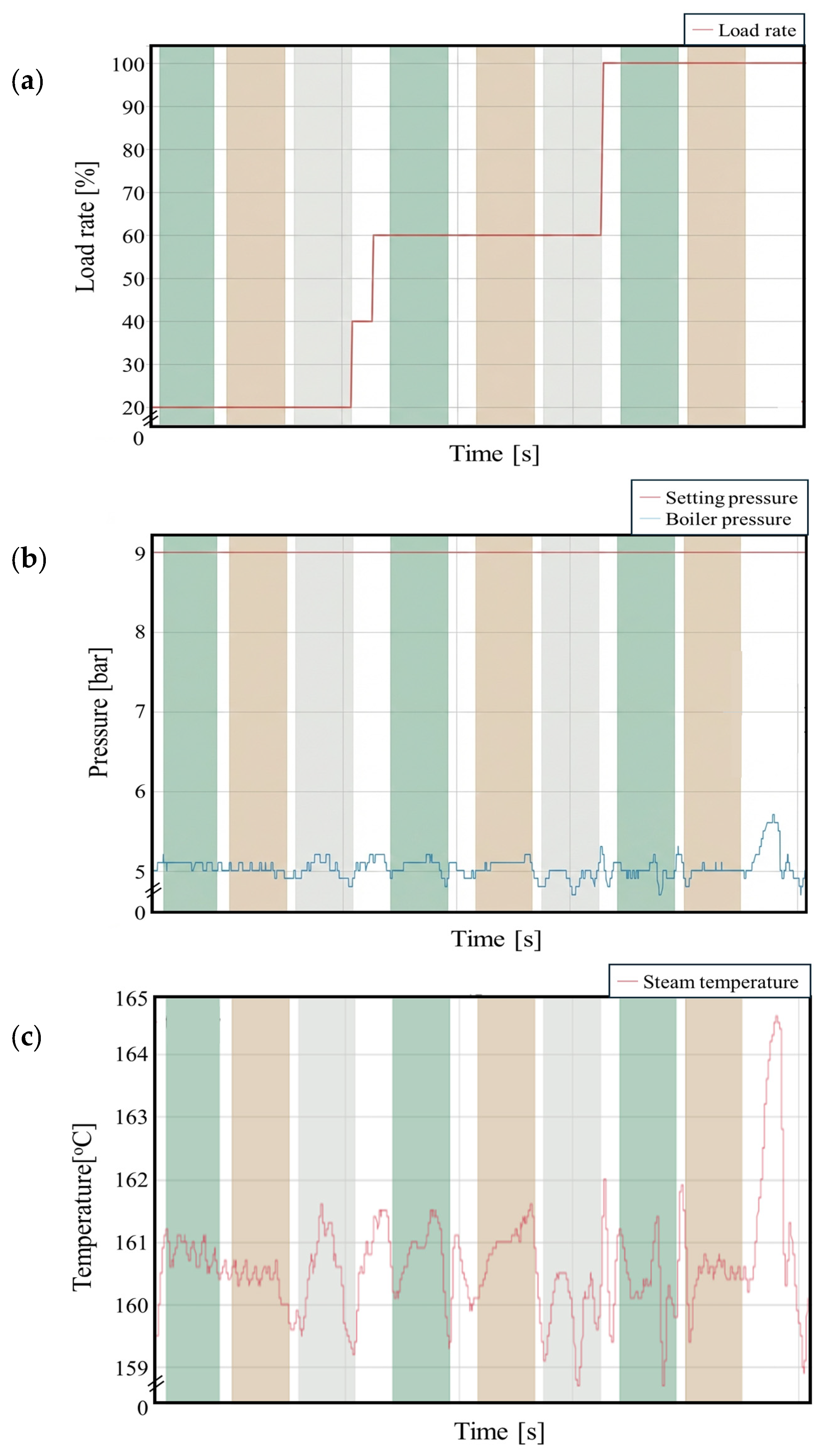
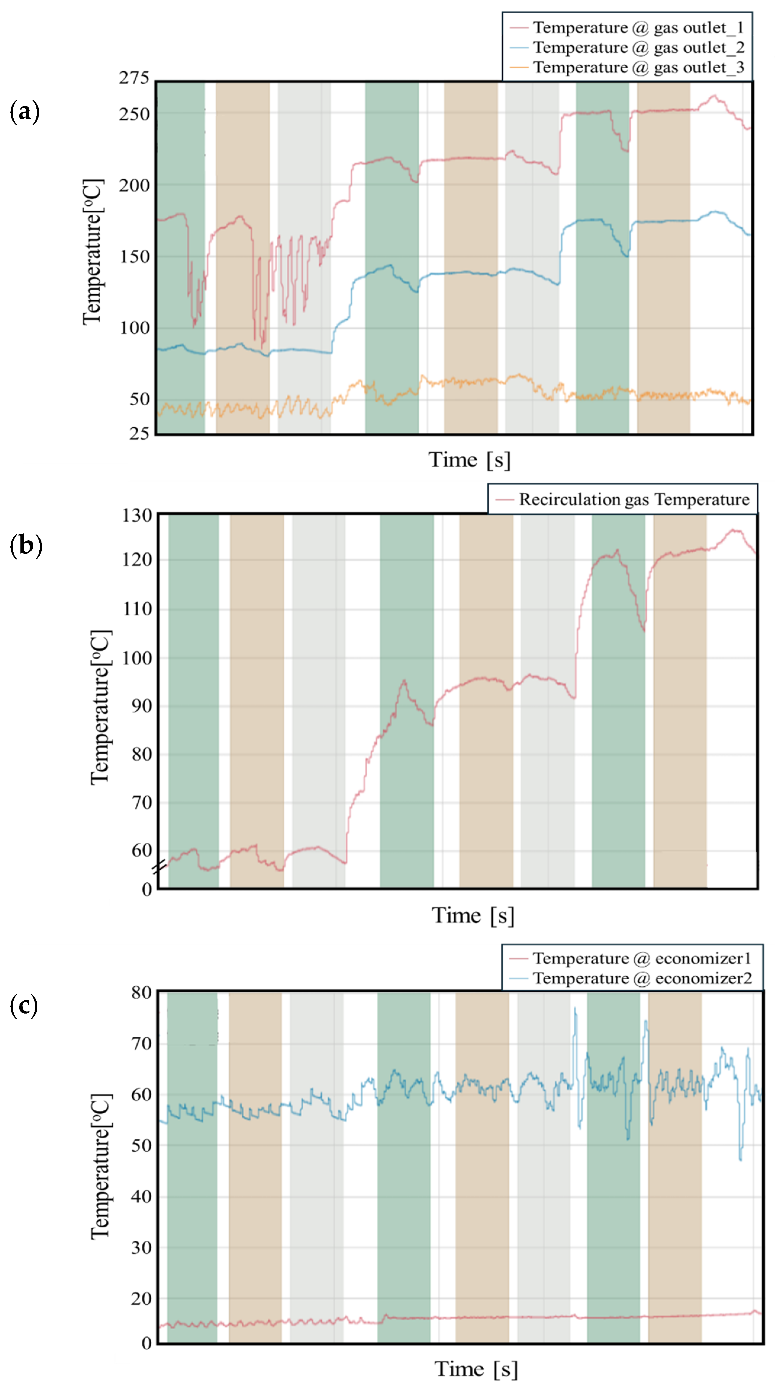
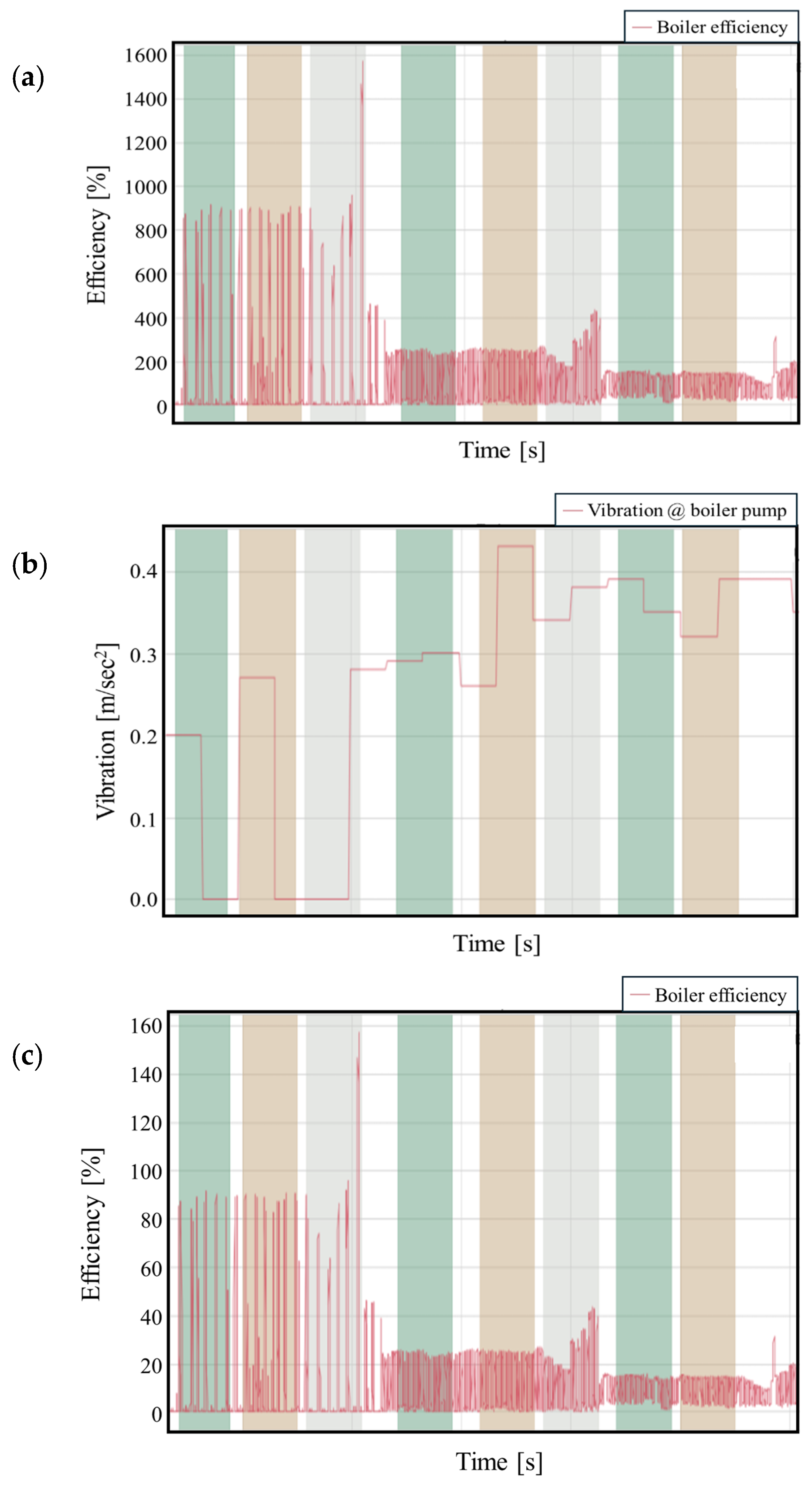
After preprocessing, the main collected datasets are visualized to examine the Load Swing and abnormal input data. The visualized results are presented in Figure 3, Figure 4 and Figure 5 and sequentially present the time-dependent load rate, steam pressure, steam temperature, outlet gas temperatures, and recirculation gas temperature, economizer water temperature, boiler efficiency, pump vibration, and blower vibration.

During normal operation, parameters in Figure 3 maintain high stability with minimal variance, providing a consistent baseline. However, during load-swing tests, the pressure and temperature exhibit predictable fluctuations that the ML model must distinguish from actual fault-induced anomalies. Figure 4 illustrates the thermal response in the gas and economizer sections. When an abnormal condition occurs, such as a reduction in combustion air, the gas temperature drops or fluctuates irregularly. The economizer temperature reflects these changes serving as a critical indicator for heat transfer efficiency degradation under fault scenarios. Figure 5 presents the normalized performance index and vibration levels. The performance index values exceeding 100% are attributed to normalization against a conservative reference baseline during transient peaks.

Following the preprocessing steps, the structured data were utilized for feature extraction and classification. To ensure reproducibility, the architectural details and hyperparameters for Autoencoder, t-SNE, and LGBM, are summarized in

Table 4. Implementation details and hyperparameters for reproducibility.

Model	Category	Specification
Autoencoder	Hidden architecture	Encoder: 128 ➔ 64, decoder: 64 ➔ 128
	Latent dimension	2 [ea]
	Optimizer/loss	Adam/mean squared error
	Epochs/batch size	100/32
t-SNE	Perplexity	30
	Learning rate	0.06
LGBM	Number of leaves	400 [ea]
	Subsample	0.8
	Minimum child weight	3
	Boosting type	Gradient boosting
	Number of Estimators	300 [ea]
	Objective	Multiclass (softmax)

. It is worth noting that most hyperparameters were maintained at their default settings to demonstrate the robustness and practical applicability of the proposed diagnostic framework without the need for extensive manual tuning.

3.3. Exploratory Data Analysis and Feature Extraction

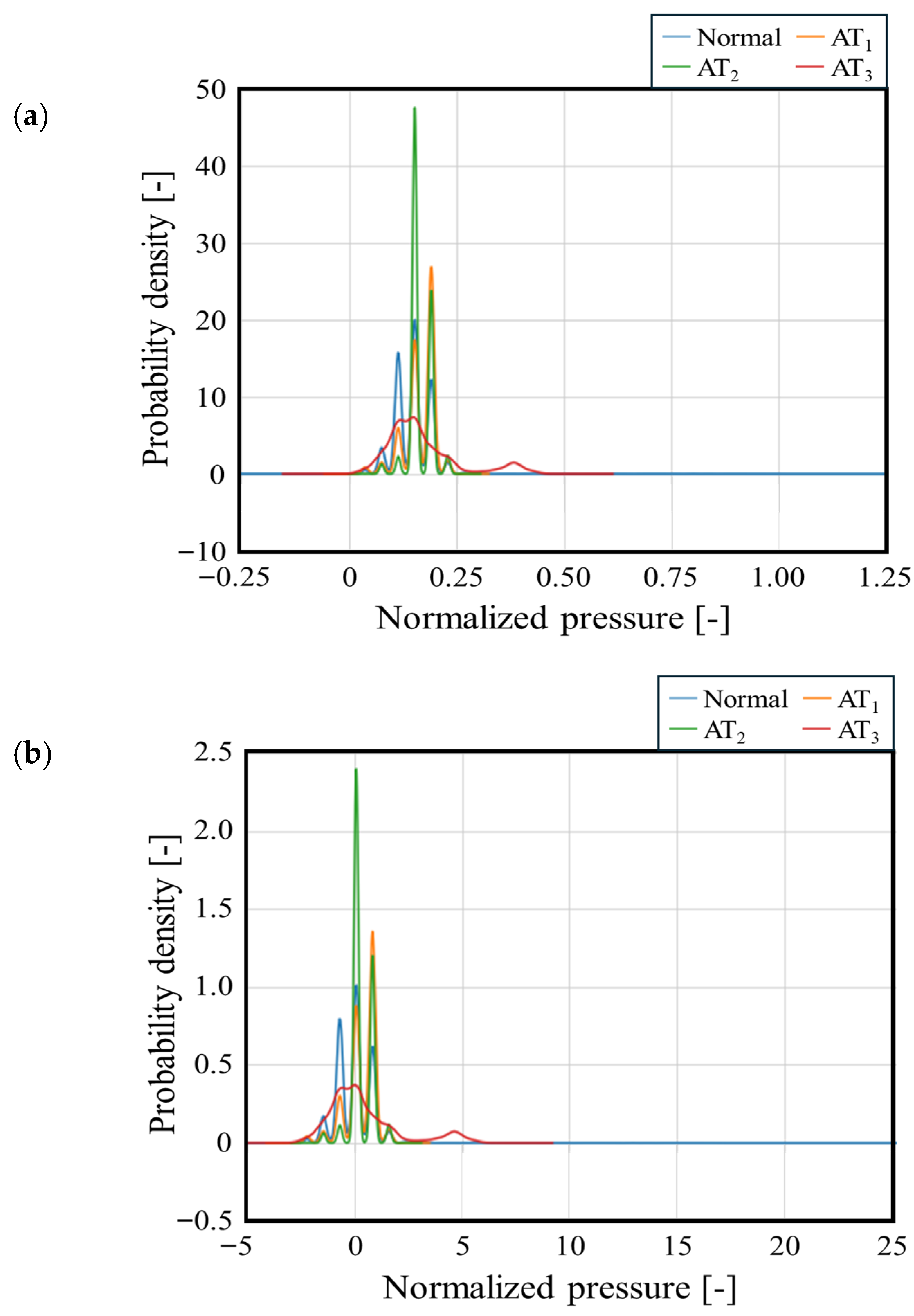
The preprocessed data are interpreted through exploratory data analysis (EDA). EDA refers to the initial stage of data analysis, where the structure, distribution, and quality of the dataset are systematically examined before modeling. In this study, EDA involves the calculation of descriptive statistics (e.g., mean, variance) and the visualization of time-series signals to identify missing values, outliers, and abnormal fluctuations. The distribution of pressure data after normalization is compared in Figure 6. Min–max scaling, Figure 6a, transforms the data into a fixed range of [0, 1], preserving the original variance but remaining highly sensitive to outliers. In contrast, standard scaling, Figure 6b re-centers the data around a zero mean with unit variance. The results show that standard scaling provides a more balanced distribution by reducing the skewness caused by extreme values, which ensures better numerical stability and faster convergence during the subsequent training of the autoencoder and LGBM models. In the graph, pressure data that can represent EDA processes are used among the data.

In addition, to closely examine the distribution of experimental data across normal and abnormal classifications, this study applies PCA [28,29]. PCA is a multivariate statistical technique that reduces the dimensionality of a dataset by transforming correlated variables into a smaller set of uncorrelated variables, referred to as principal components.

Mathematically, the process begins by standardizing the dataset and computing its covariance matrix Σ. The covariance structure is then decomposed through eigenvalue analysis:

$$\sum v_i={\lambda }_i{v}_i$$

(1)

where λ represents the eigenvalues, indicating the amount of variance explained, and $v_i$ shows the corresponding eigenvectors, which define the directions of maximum variance. The principal components are obtained by projecting the original data onto these eigenvectors:

Z = XV

(2)

where V = [$v_1$, $v_2$, …, $v_k$] is the matrix of eigenvectors corresponding to the top k eigenvalues.

In this way, the first principal component accounts for the greatest variance in the dataset, the second accounts for the next greatest variance orthogonal to the first, and so on. By selecting the top two or three components, the method enables effective visualization and pattern recognition while retaining most of the information contained in the original data.

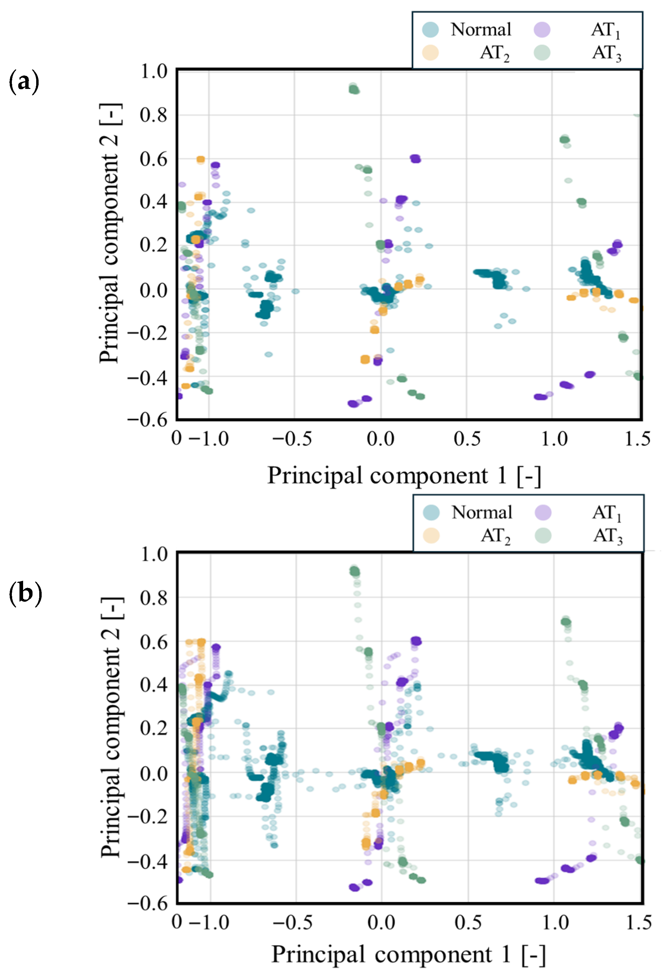
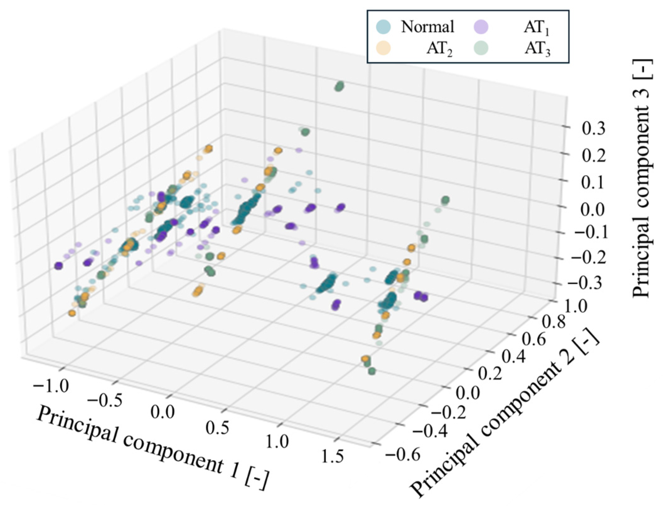
The results of the two-dimensional PCA transformation are presented in Figure 7, where most of the normal data are separated from abnormal data, though some overlap exists. This overlap is observed both in the 100% load dataset and in the 20% load dataset. To further improve separability, a three-dimensional PCA is additionally performed, as shown in Figure 8, which demonstrated clearer distinction between normal and abnormal states.

While PCA effectively captures the global variance, its linear nature often fails to preserve the complex local structures of high-dimensional measured data. To overcome this limitation and better examine the local neighborhood relationships that PCA might overlook, t-SNE is subsequently conducted as a nonlinear dimensionality reduction method. In this study, t-SNE and autoencoders were employed strictly for EDA to confirm the inherent separability of the boiler’s operating states before constructing the final diagnostic model. These techniques serve as visualization and feature extraction tools to justify the feasibility of the classification task, rather than functioning as standalone diagnostic methods. As a nonlinear dimensionality reduction method designed primarily for visualization [30], t-SNE converts the pairwise distances between data points in the high-dimensional space into neighbor-affinity probabilities, where closer points have higher similarity values. These similarities in the original space are modeled by a Gaussian distribution, as described in Equation (3).

$$KL\left(P‖Q\right)=\sum _i\sum _j{p}_{ij}log{\displaystyle \frac{p_{ij}}{q_{ij}}}$$

(3)

where $p_{ij}$ denotes the similarity between points $i$ and $j$ in the high-dimensional space and $q_{ij}$ represents their similarity in the low-dimensional embedding.

Next, t-SNE constructs a two or three-dimensional embedding that preserves these neighbor relationships from the original data. As a result, t-SNE focuses on preserving local neighborhoods; t-SNE keeps nearby points in the original data close in the embedding, rather than trying to maintain exact global distances. This makes t-SNE particularly useful for visually examining whether normal and abnormal operating states form distinct clusters. For practical use, the data are standardized and optionally reduced with PCA to a moderate number of components to denoise and accelerate optimization. Key hyperparameters which define the effective neighborhood size, and the learning rate are adjusted within typical ranges, and multiple random initializations are used to ensure stability.

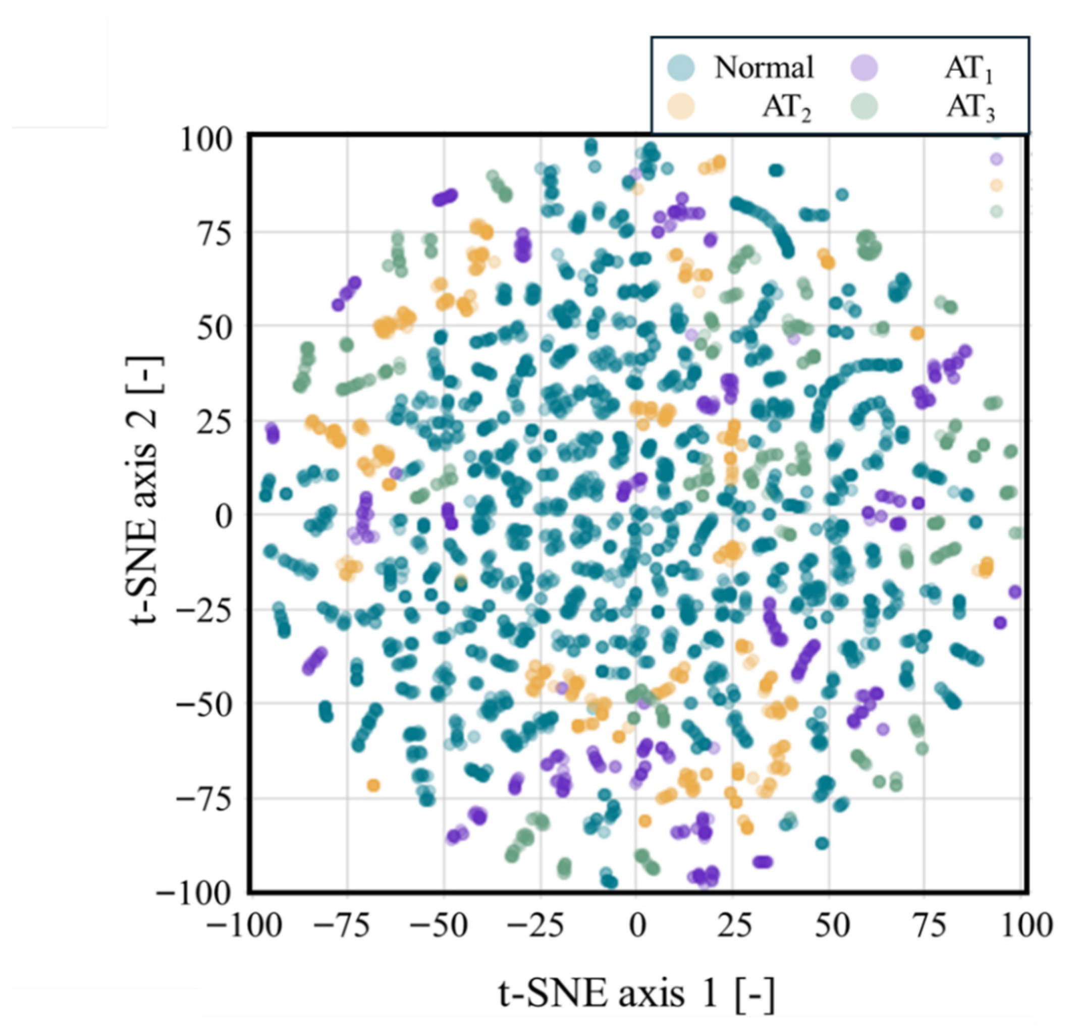
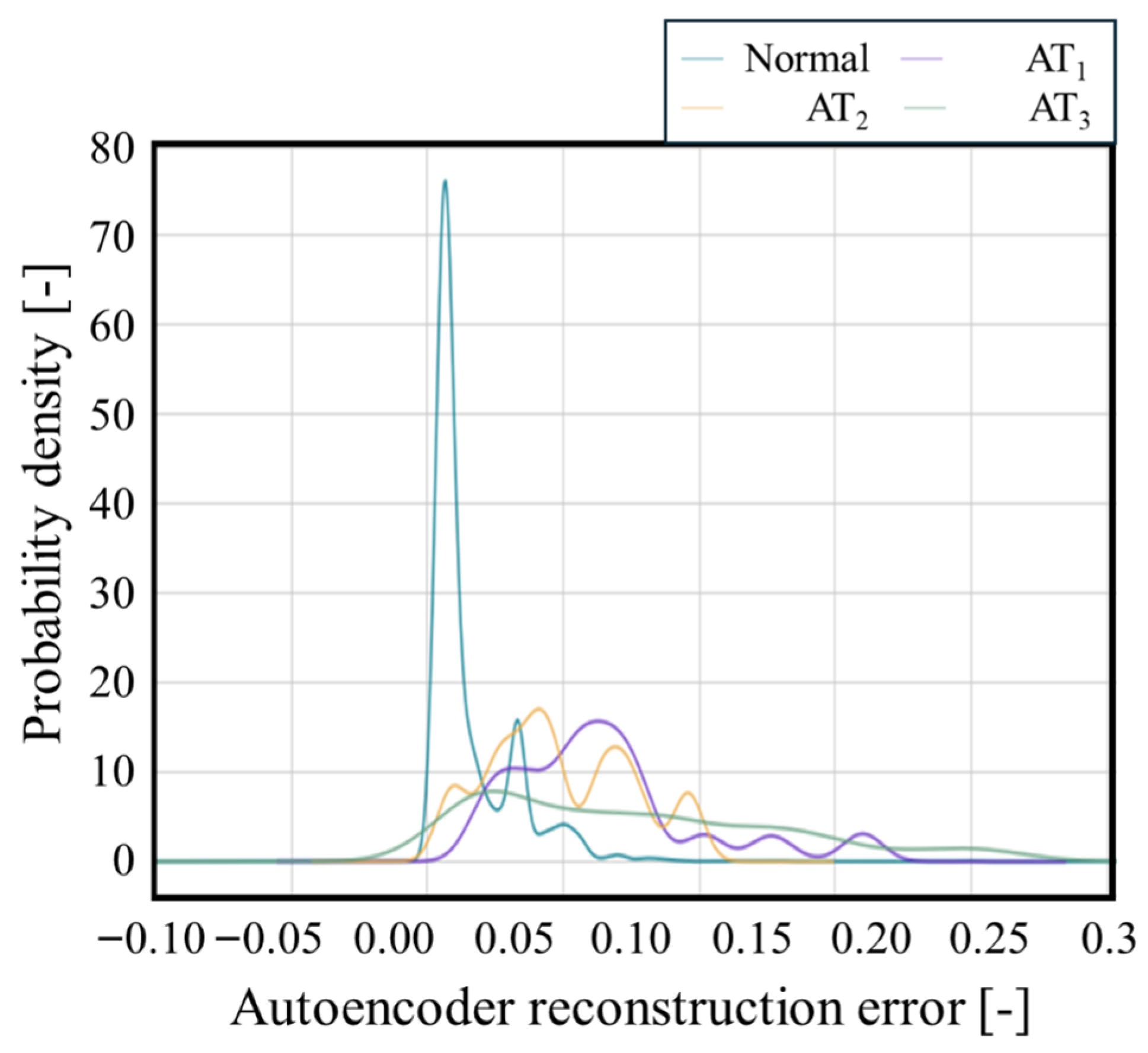
t-SNE visualization shows that the overlap between normal and abnormal samples is relatively small. However, the data points remain widely scattered rather than forming compact clusters as Figure 9. This result suggests that neighborhood-preserving embedding alone is insufficient for clear class separation under certain operating conditions. While t-SNE provides valuable insights into local clusters, its utility is primarily limited to exploratory visualization, as it lacks a functional mapping for new data points and often results in widely scattered distributions. To transition from qualitative visualization to a more robust and trainable feature representation, an autoencoder is employed. This neural network architecture compresses input data into a low-dimensional latent space and subsequently reconstructs it, enabling the model to learn compact, nonlinear relationships inherent in the data. By prioritizing reconstruction accuracy, the autoencoder facilitates a clearer differentiation between normal and abnormal operating states through both latent feature clusters and quantitative reconstruction errors. Compared with the analysis based on t-SNE only, the autoencoder provides a clearer clustering of normal data, although some regions still exhibit dispersed distributions [31]. The error-rate graph derived from the autoencoder process, which defines the difference between input and output data during encoding and decoding as reconstruction error, is presented in Figure 10. Additionally, autoencoder error rate density analysis shows that the reconstruction error for normal data remains small and is concentrated near zero, whereas abnormal data display larger error values in Figure 10. This result confirms that the distributional differences between normal and abnormal data can be identified, enabling their separation. However, when comparing abnormal cases across AT₁–AT₃, the distributions do not exhibit consistent or distinguishable patterns, indicating that classification among specific fault causes is difficult.

3.4. Model Training and Performance Evaluation with LGBM

The preceding manifold learning analyses (PCA, t-SNE, and Autoencoders) collectively revealed that while normal and abnormal states are distinguishable, they exhibit significant overlapping regions that pose a ‘classification challenge’. While these techniques provided qualitative insights into data separability, the LGBM algorithm was implemented as the final and only diagnostic model. Unlike exploratory visualization and feature extraction tools, LGBM establishes the rigorous decision rules necessary for definitive anomaly detection and classification.

While deep learning architectures such as CNNs and RNNs were considered, the LGBM-based ensemble model was ultimately selected for this diagnostic framework. Unlike CNNs, which excel in spatial pattern recognition, or RNNs, which are optimized for long-term temporal dependencies, LGBM provides superior robust performance on structured tabular sensor data with lower computational overhead. In industrial settings, the ability to process high-dimensional data with high interpretability and minimal tuning is a significant advantage, and comparative analysis of feature extraction methods in this study further validates this choice as a functional ablation study.

Based on these insights, which confirm the nonlinear complexity of the dataset, the Light Gradient Boosting Machine (LGBM) is selected for the final classification task [32,33]. LGBM is chosen for its superior ability to handle such complex decision boundaries and its robustness against overfitting in high-dimensional industrial datasets. As a tree-based ensemble learning method that belongs to the family of gradient boosting algorithms, LGBM improves classification performance by combining many simple decision trees, where each tree is trained to correct the errors of the previous ones. This sequential learning strategy enables the model to capture nonlinear patterns in complex datasets with high accuracy and efficiency.

The principle of gradient boosting is expressed in Equation (4).

$$M^{\left(t\right)}\left(x\right)=M^{\left(t-1\right)}\left(x\right)+{\eta h}_t\left(x\right)$$

(4)

where $M^{\left(t\right)}\left(x\right)$ denotes the prediction after t iterations, $h_t\left(x\right)$ is the newly constructed decision tree, and $\eta$ is the learning rate that controls the contribution of each tree.

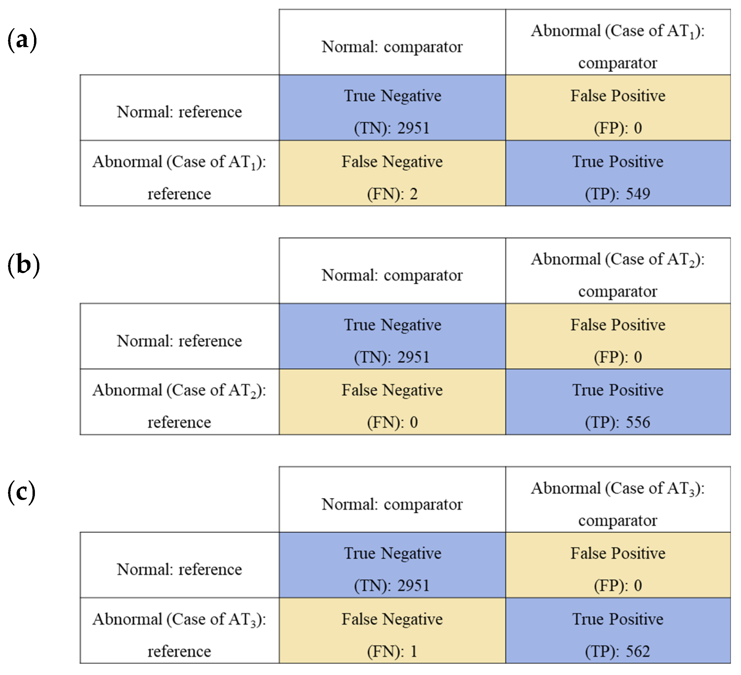
Compared with conventional gradient boosting methods, LGBM is optimized for speed and memory usage through a histogram-based algorithm and a leaf-wise tree growth strategy. LGBM is particularly suitable for handling large sensor datasets obtained from industrial systems such as boilers due to its superior speed and memory efficiency. The classification results obtained from LGBM are evaluated using a confusion matrix, which summarizes the numbers of correctly and incorrectly classified samples and is shown as Figure 11 [26,40,41,42,43]. This evaluation allows a clear assessment of the model’s ability to distinguish between normal and abnormal operating states. To prevent data leakage, the dataset was split time-based rather than randomly, with the first 80% of each experimental segment used for training and the remaining 20% held out for testing. By employing a chronological split across a multi-day dataset, the testing set predominantly contains samples from the final stages of the experiment. This ensures that the model is evaluated on temporally disjoint data, thereby mitigating the risk of overestimation associated with same-day, highly correlated measurements. This approach maintains the temporal order and ensures statistical independence, providing a rigorous assessment of the model’s performance on truly unseen sequences. In this study, only the most relevant details are repeated.

Based on the analysis using the confusion matrix, four adequacy indicators are calculated: ACCURACY, PRECISION, RECALL, and F1-SCORE. The most notable indicators are ACCURACY and RECALL, which include false negative (FN), when the reference detected an abnormality, but the comparator determined it to be normal. In this study, FN refers to cases where the diagnostic method determines the operation as normal even though an abnormal operation is actually occurring. If such cases continue, the risk of accidents becomes higher than in other cases; therefore, FN was considered an important parameter.

The confusion matrix results shown in Figure 11 exhibited high indicator values in all cases from (1)–(3). In Figure 11a (AT₁), ACCURACY = 99.94% and RECALL = 99.64%; in Figure 11b (AT₂), both ACCURACY and RECALL reached 100%; and in Figure 11c (AT₃), ACCURACY = 99.97% and RECALL = 99.82%. These results indicate that the proposed method classifies the abnormal operating conditions of the boiler with considerably high adequacy.

However, such results may also be influenced by issues such as model overfitting, which can artificially inflate accuracy. In this study, LGBM is adopted because of its relatively low susceptibility to overfitting compared with other ML models. Nevertheless, LGBM should be noted that LGBM does not eliminate the risk of overfitting completely, and further validation is needed in future studies to ensure the robustness and generalizability of the model. In addition, this study faced a limitation regarding the measurement interval of boiler data. This irregularity was primarily due to the fact that the sensors installed in the boiler are not precision-grade instruments designed for experimental research but rather standard industrial sensors. Consequently, the non-uniform sampling intervals may have introduced bias or reduced the resolution of dynamic state detection, indicating the need for improved data acquisition systems in further studies.

4. Conclusions

This study investigates an ML-based approach for diagnosing boiler abnormalities, focusing on the model’s response to various abnormal scenarios. Unlike existing methods often constrained to narrow operating conditions, this research fills the gap by validating the diagnostic framework across a wide load range of 20% to 100% using load-swing tests. The main findings and their implications are summarized.

Firstly, the proposed model was successfully trained and evaluated using variate operational data from a 5-ton field demonstration boiler in South Korea. This confirms its capability to reliably distinguish between normal and abnormal states in industrial environments.

Second, based on a large-scale dataset of 28,943 samples measured from experimental facility, the LGBM-based ensemble approach demonstrated significant academic value by achieving a minimum classification accuracy of 99.64%.

Third, while 2D/3D PCA and t-SNE visualizations revealed complex overlapping regions between states, the LGBM model maintained high performance. This ability to handle inherently challenging data structures represents a core innovation in this study.

Fourth, the reliability of these high-accuracy results was rigorously verified through a chronological validation strategy. The consistent performance observed between training and testing sets confirms that the model is robust against overfitting, effectively generalizing to unseen temporal sequences.

Fifth, while the current dataset was collected under real field conditions, certain irregularities in the measurement intervals were observed. Furthermore, as the data for this study were obtained from a specific 5-ton boiler, further validation is needed to generalize the model to boilers of various types and capacities. Future research will aim to verify the versatility of the model across different industrial boiler environments, while also focusing on improving data integrity by ensuring consistent sampling intervals and incorporating long-term data from various commercial systems.

Finally, the practical significance of this research lies in its potential to enhance industrial safety and economic efficiency. By enabling early detection of anomalies like pressure vessel ruptures, this framework can significantly reduce unplanned downtime, mitigate catastrophic accident risks, and prevent energy losses caused by decreased thermal efficiency. Ultimately, this work provides a critical foundation for sustainable energy management and predictive maintenance in industrial heating applications.