SKNet-GAT: A Novel Multi-Source Data Fusion Approach for Distribution Network State Estimation

Abstract

This paper tackles the growing uncertainty in distribution networks caused by distributed generation, load fluctuations, and frequent topological changes. It proposes a multi-source data fusion framework using enhanced selective convolution (SKNet) and graph attention networks (GAT). First, heterogeneous measurement data, including Phasor Measurement Unit (PMU) and Supervisory Control and Data Acquisition (SCADA) data, are processed through a unified normalization and outlier elimination technique to ensure data quality. Second, SKNet is utilized to extract spatiotemporal multi-scale features, improving the detection of both rapid disturbances and long-term trends. Third, the extracted features are fed into GAT to model node electrical couplings, while power flow residual constraints are embedded in the loss function to enforce the physical validity of the estimated states. This physics-informed design overcomes a key limitation of pure data-driven models and enables an end-to-end framework that integrates data-driven learning with physical mechanism constraints. Finally, comprehensive validation is performed on the improved IEEE 33-node and IEEE 123-node test systems. The test scenarios include Gaussian measurement noise, data outliers, missing measurements, and topological changes. The results show that the proposed method outperforms baseline models such as Multi-Scale Graph Attention Network (MS-GAT), Bidirectional Long Short-Term Memory (BiLSTM), and traditional weighted least squares (WLS). It achieves Root Mean Square Error (RMSE) reductions of up to 18% and Mean Absolute Error (MAE) reductions of up to 15%. The average inference latency is only 10–18 ms. Even under unknown topological changes, the estimation error increases by only 15–25%. These results demonstrate the superior accuracy, robustness, and real-time performance of the proposed method for intelligent distribution network state estimation.

1. Introduction

Distribution network state estimation plays a vital role in maintaining the safe and stable functioning of the power grid. As distributed energy sources are increasingly integrated, the dynamics of distribution networks have become more complex, resulting in greater load fluctuations [1]. This results in higher demands on both the accuracy and real-time performance of state estimation [2,3]. Traditional distribution network state estimation has primarily relied on measurements from control and monitoring systems [4], which capture electrical quantities. These systems have long served as the primary data source for distribution network operation and analysis. In recent years, advanced measurement devices have been integrated into distribution networks [5], providing high-precision, time-synchronized data to support more accurate and responsive system analysis. However, the relatively low sampling frequency of SCADA data hinders capturing the distribution network’s rapid dynamic changes. Meanwhile, the high deployment cost and limited coverage of PMUs remain prominent challenges.

In traditional distribution network state estimation, classical optimization-based methods have played a central role [6]. These methods determine the system state by minimizing the weighted sum of squares of measurement residuals. They provide more accurate results when sufficient data are available and noise levels are low [7,8]. However, distribution networks have unique structural and operational characteristics that present significant challenges. Sparse measurement points, dynamic topological changes, and the volatility of distributed power sources complicate the estimation process [9]. Unlike transmission networks, distribution networks are less densely monitored, and frequent topology changes can cause estimation errors that quickly propagate due to electrical coupling [10]. Additionally, the integration of distributed energy sources introduces further complexity because of their intermittent and volatile nature, rendering traditional static models insufficient for accurate state estimation.

In recent years, data-driven methods based on artificial intelligence and machine learning have been increasingly explored to enhance the performance of distribution network state estimation. Representative models, including recurrent architectures [11], graph-based learning frameworks [12], convolutional neural structures [13], and long-term temporal modeling networks [14], have shown promising results. For instance, a neural network-based state estimation method, when combined with linear optimization, successfully integrates data from PMUs and SCADA systems, addressing topology changes and noise interference [15]. However, these methods primarily rely on single-scale modeling, which cannot fully capture the multi-scale fluctuations caused by distributed energy integration. In distribution networks, state variables such as voltage and current exhibit both short-term random disturbances and long-term trends, requiring multi-scale modeling to improve estimation accuracy [16,17].

Existing multi-source state estimation methods often struggle to jointly capture fast transients and long-term trends while accurately modeling spatial correlations, as many approaches either prioritize one type of temporal feature or lack effective fusion mechanisms across heterogeneous measurements [18]. Simple PMU/SCADA concatenation or weighted averaging treats high-frequency PMU events and low-frequency SCADA trends equally, causing mutual interference [19]. Fixed-scale multi-source models like SK-BiLSTM cannot adaptively balance transient and trend features, and graph-based methods such as MS-GAT focus on spatial dependencies but neglect temporal multi-scale dynamics [20]. In contrast, SKNet-GAT uses selective kernel convolution to adaptively fuse multi-scale temporal features from PMU and SCADA data while leveraging GAT for spatial modeling, effectively capturing both fast and slow dynamics and addressing the key limitations of existing fusion techniques [21].

A new multi-source data fusion approach is presented, and the main contributions are outlined below:

1.

We introduce an enhanced Selective Kernel Convolutional Neural Network (SKNet) integrated with a Graph Attention Network (GAT), which effectively addresses the integration of heterogeneous data sources. SKNet adapts to both local and global electrical features by leveraging multi-scale convolution and a selective kernel mechanism.

2.

The GAT is employed to model the electrical coupling relationships between network nodes. By incorporating system topology and temporal measurements, it captures the spatiotemporal dependencies and interactions between nodes more effectively than traditional methods.

3.

We integrate power flow residual constraints into the loss function to form a physics-informed dynamic model, ensuring physically valid power flow solutions and addressing a key limitation of pure data-driven DL methods. Combined with time-evolving state constraints, this design enables robust adaptation to load fluctuations and topology changes, enhancing practical applicability.

4.

The proposed method significantly improves the accuracy, robustness, and key node identification capabilities of state estimation, providing better support for real-time situational awareness in intelligent distribution networks. This contributes to enhanced monitoring, optimized operation, and effective fault prediction and management.

2. Related Work

2.1. Spatiotemporal Characteristics and SKConvolution in State Estimation

Distribution network state estimation faces significant challenges due to nonlinearity, time variation, and multi-scale coupling. Node voltage and power flow data exhibit complex spatiotemporal behaviors, influenced by load fluctuations, renewable energy integration, and operational trends [22]. Additionally, frequent topology changes lead to both local and distant electrical couplings, further complicating state estimation. These factors result in issues such as sparse measurements, noise interference, and topological uncertainty [23].

The Selective Kernel Convolutional Neural Network (SKNet) addresses these challenges by using multi-scale convolutions combined with adaptive weighted selection. The input feature set $\{K_1,K_2,\dots ,K_m\}$ is convolved with different kernels at varying scales to generate multi-scale responses $\{U_1,U_2,\dots ,U_m\}$. The selective weights $\alpha =\{{\alpha }_1,{\alpha }_2,\dots ,{\alpha }_m\}$ are adaptively learned through a gating mechanism, and the normalization condition is applied to ensure the sum of the weights equals 1:

$$\sum _{i=1}^m{\alpha }_i=1,{\alpha }_i\in [0,1],\forall i\in \{1,2,\dots ,m\}$$

(1)

Next, the multi-scale responses $U_i$ are aggregated with the selective weights ${\alpha }_i$ to compute the final output Y, which is then regularized to prevent overfitting and improve generalization. This is achieved by adding a regularization term $\lambda {\sum }_{i=1}^m{\alpha }_i^2$ that penalizes large weights, where $\lambda \in {\mathbb{R}}^{+}$ controls the weight penalty and encourages sparsity in the learned feature representations:

$$Y=\sum _{i=1}^m{\alpha }_i·U_i+\lambda \sum _{i=1}^m{\alpha }_i^2,\lambda \in {\mathbb{R}}^{+}$$

(2)

where $\lambda \in {\mathbb{R}}^{+}$ is a regularization coefficient that regulates the weight penalty, encouraging sparsity in the learned feature representations and limiting the contribution to the final output to informative features only.

Lastly, each convolution operation is applied to the input features $K_i$ using a distinct kernel $W_i$, resulting in the multi-scale feature maps $U_i$. The convolution operation is defined as:

$$U_i=\sum _{j=1}^n{K}_i\left[j\right]·W_i\left[j\right],\forall i\in \{1,2,\dots ,m\}$$

(3)

where $K_i\left[j\right]$ and $W_i\left[j\right]$ represent the j-th element of the input feature $K_i$ and the convolution kernel $W_i$, respectively, and n is the size of the kernel. This allows SKNet to capture multi-scale features and learn spatial dependencies at different resolutions. This mechanism enables the model to represent transient fluctuations as well as persistent patterns, while balancing local and global spatial features. As shown in Figure 1, Selective Kernel Convolution (SKConv) enhances dynamic modeling, robustness to noise, and adaptability to topology changes through multi-scale feature fusion.

2.2. Construction Principle of State Estimation Model

Although SKConv has advantages in multi-scale feature modeling, it remains fundamentally a convolution operation. Its utilization of complex topological structures is inadequate, which hinders its ability to fully capture the non-Euclidean electrical coupling relationships between nodes in the distribution network [24]. Moreover, convolution has limited ability to capture extended temporal patterns, and generalization and stability can still degrade under measurement loss or noise interference. To mitigate these issues, a GAT [25] is based on SKConv, aiming to achieve a deep fusion of topological structure information and dynamic measurement data.

Specifically, first, SKConv is employed to capture multi-scale dynamic features, allowing the model to better capture both local variations and global trends. Subsequently, these features are input into GAT, where the importance of neighboring nodes is adaptively weighted through an attention mechanism to facilitate spatial dependency modeling at the node level. Finally, the residual of the power flow equation is included in the loss function to guarantee that the estimation results respect the physical laws of the power system [26]. This combined framework can effectively improve the robustness and generalization capability of state estimation under conditions of topology switching, measurement loss, and noise interference.The structure of the GAT is depicted in Figure 2.

The basic principle of GAT is as follows:

• Feature concatenation: The initial feature vectors of nodes are obtained by concatenating dynamic measurements and topological features. The product combines physical measurements with network structure information to construct a more comprehensive feature representation for each node:

  $$h_i=\left[x_i\Vert y_i\right],\mathrm{where}{x}_i\in {\mathbb{R}}^{d_1}\mathrm{and}{y}_i\in {\mathbb{R}}^{d_2}$$

  (4)

  where $x_i\in {\mathbb{R}}^{d_1}$ and $y_i\in {\mathbb{R}}^{d_2}$ denote the dynamic measurement and topological feature vectors of node i.
• Linear transformation: The initial node eigenvectors $h_i$ are transformed into a new feature space by applying a learned weight matrix W:

  $$h_i^{\prime }=W{h}_i+b_i,W\in {\mathbb{R}}^{d^{\prime }\times (d_1+d_2)},b_i\in {\mathbb{R}}^{d^{\prime }}$$

  (5)

  where W is the transformation matrix that projects the concatenated features $h_i$ into a new feature space of dimension $d^{\prime }$, and $b_i$ is the bias vector associated with the transformation. Here, $h_i^{\prime }$ is the feature vector of node i after the linear transformation, and $d^{\prime }$ denotes the dimension of the transformed feature space.
• Attention Coefficient Calculation:Compute the influence score of a neighboring node on the current central node. The model adapts the strength of the correlation between two nodes based on their composite features (operating state + topology):

  $$e_{ij}=\mathrm{LeakyReLU}\left({\mathbf{a}}^T\left[h_i^{\prime }\Vert h_j^{\prime }\right]\right),\mathbf{a}\in {\mathbb{R}}^{2d^{\prime }}$$

  (6)

  where $\mathbf{a}$ is a learnable attention vector and LeakyReLU serves as a non-linear activation, computing the attention score $e_{ij}$ from the concatenated transformed feature vectors of nodes i and j. Here, $\mathbf{a}\in {\mathbb{R}}^{2d^{\prime }}$ is the learnable attention vector, and $[h_i^{\prime }\parallel h_j^{\prime }]$ denotes the concatenation of the transformed features of nodes i and j, which serves as the input to the LeakyReLU activation.
• Normalization Process: Normalize all the attention coefficients calculated in the previous step to convert them into a probability distribution:

  $${\alpha }_{ij}={\displaystyle \frac{exp\left(e_{ij}\right)}{{\sum }_{k\in N_i}exp\left(e_{ik}\right)}},\sum _{j\in N_i}{\alpha }_{ij}=1$$

  (7)

  where $N_i$ is the set of node i’s neighbors, with ${\alpha }_{ij}$ normalized to form a probability distribution.
• Feature Aggregation: Nodes exchange and integrate information through their connection relationships (edges), generating a new feature representation that captures their local neighborhood context. The aggregation process takes the attention-weighted sum of the neighboring features:

  $$h_i^{\prime \prime }=\sigma \left(\sum _{j\in N_i}{\alpha }_{ij}W{h}_j+b_i\right),\sigma (·)\mathrm{is}\mathrm{the}\mathrm{activation}\mathrm{function}$$

  (8)

  where $W{h}_j$ represents the transformed feature vector of neighboring node j, and $\sigma (·)$ is a non-linear activation function. The output $h_i^{\prime \prime }$ is the updated feature representation for node i, which aggregates the weighted information from its neighbors.

Through this mechanism, GAT adaptively assigns importance to neighboring nodes, enhancing the model’s adaptability to complex topologies. Combined with SKConv, it organically integrates multi-scale feature extraction, topological modeling, and physical constraints, ensuring high accuracy and robustness under complex conditions.

3. Methodology

3.1. State Estimation via SKNet–GAT Multi-Source Data Fusion

The proposed SKNet–GAT multi-source fusion state estimation framework is illustrated in Figure 3. The overall architecture consists of five sequentially connected modules, namely the input preprocessing layer, SK-based multi-scale feature extraction layer, GAT-based topology fusion layer, physical consistency constraint layer, and estimation output layer. Each module is designed to collaboratively exploit temporal dynamics, spatial dependencies, and physical mechanisms of distribution networks.

1.

Input preprocessing layer:

Measurements from PMUs and SCADA systems, along with topological features like node degree, switch status, and electrical distance, are preprocessed to handle missing values, noise, and inconsistent scales [27]. After normalization and time alignment, the data are organized into a unified high-dimensional tensor [28].

$$\mathbf{X}=\left\{{\mathbf{x}}_{t,i,c}\right\}\in {\mathbb{R}}^{T\times N\times C},{\mathbf{x}}_{t,i,c}={\displaystyle \frac{x_{t,i,c}-x_c^{min}}{x_c^{max}-x_c^{min}}},$$

(9)

where T denotes the time window length, N is the number of nodes, C represents the number of measurement channels, and $x_c^{min}$, $x_c^{max}$ are the minimum and maximum values of channel c, respectively.

2.

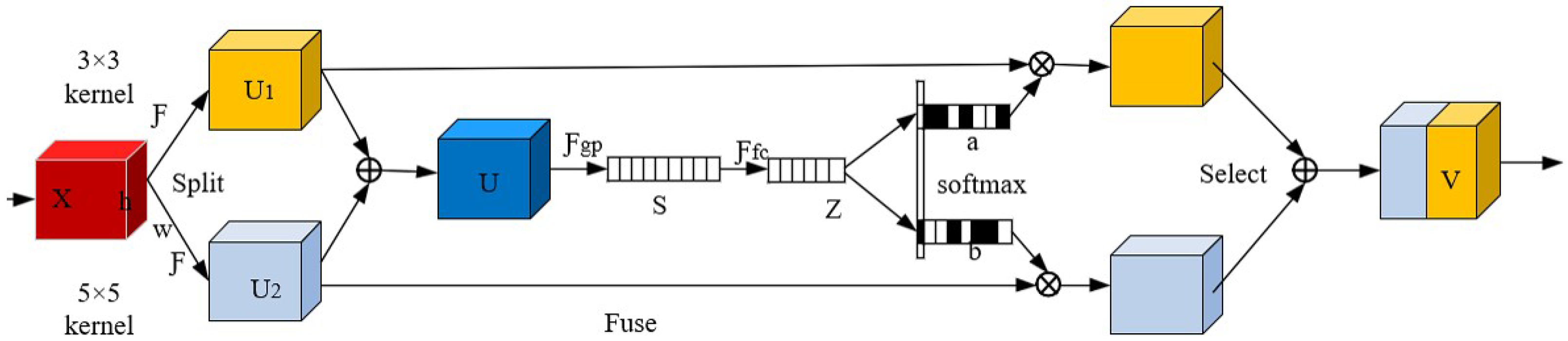
SK multi-scale feature extraction layer: To capture temporal dynamics at different resolutions, multiple convolution kernels with distinct receptive fields are applied in parallel. The multi-scale features are adaptively fused through a selective kernel mechanism:

$$\mathbf{U}=\sum _{k=1}^K{\alpha }_k·{\varphi }_k\left({\mathbf{W}}_k\ast \mathbf{X}+{\mathbf{b}}_k\right),{\alpha }_k={\displaystyle \frac{exp\left(s_k\right)}{{\sum }_{l=1}^{K}exp\left(s_l\right)}},$$

(10)

where ∗ denotes convolution, ${\varphi }_k(·)$ is the nonlinear activation function, ${\mathbf{W}}_k$ and ${\mathbf{b}}_k$ are the kernel parameters, and ${\alpha }_k$ are dynamically learned gating weights generated via global pooling and channel-wise attention. This mechanism enables soft fusion of heterogeneous measurements while emphasizing informative temporal patterns.

3.

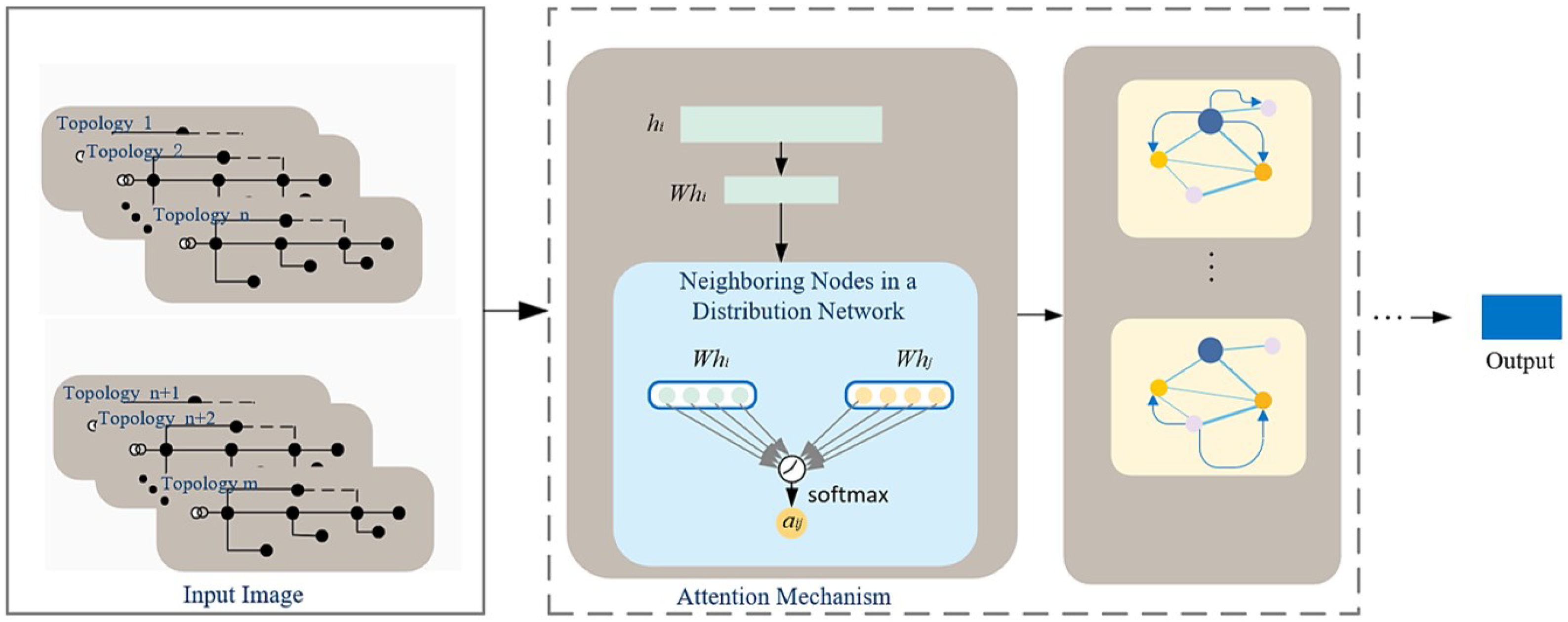
GAT topology fusion layer: Based on the electrical adjacency matrix, the extracted temporal features are further aggregated using a graph attention mechanism to explicitly model non-Euclidean electrical coupling among nodes:

$${\mathbf{H}}_i=\sigma \left(\sum _{j\in {\mathcal{N}}_i}{\displaystyle \frac{exp\left(\mathrm{LeakyReLU}\left({\mathbf{a}}^{\top }[\mathbf{W}{\mathbf{U}}_i\Vert \mathbf{W}{\mathbf{U}}_j]\right)\right)}{{\sum }_{k\in {\mathcal{N}}_i}exp\left(\mathrm{LeakyReLU}\left({\mathbf{a}}^{\top }[\mathbf{W}{\mathbf{U}}_i\Vert \mathbf{W}{\mathbf{U}}_k]\right)\right)}}\mathbf{W}{\mathbf{U}}_j\right),$$

(11)

where $\mathbf{a}$ is a learnable attention vector, ${\mathcal{N}}_i$ the set of neighbors, and ${\mathbf{H}}_i$ the topology-aware embedding for node i.

4.

Physical consistency constraint layer: To ensure data-driven estimation results comply with power system physical laws, the training objective incorporates power flow equation residuals. The loss function is defined as:

$$\mathcal{L}={\displaystyle \frac{1}{N}}\sum _{i=1}^N{\rho }_{\delta }\left({\hat{x}}_i-x_i\right)+\lambda {∥\mathbf{f}(\hat{\mathbf{x}},\mathbf{Y})∥}_2^2,$$

(12)

where ${\rho }_{\delta }(·)$ denotes the Huber loss, $\mathbf{f}(·)$ represents the nonlinear power flow equations, and $\lambda$ controls the strength of the physical regularization term.

5.

Estimation output layer: Finally, the fused spatiotemporal features are mapped to nodal voltage magnitudes and phase angles through a fully connected projection. Evaluation metrics such as MAE, RMSE, $R^2$, and inference latency are synchronously computed to support real-time dispatching and situational awareness applications.

To highlight the novelty of the proposed SKNet–GAT integration, a concise comparison with the state-of-the-art MS-GAT (multi-scale graph attention network) is provided: (i) Feature extraction: MS-GAT uses fixed-scale graph convolution, while SKNet–GAT integrates SKNet to adaptively fuse multi-scale temporal features (short-term disturbances and long-term trends) via a selective kernel mechanism, addressing multi-scale fluctuations in distribution networks. (ii) Topology modeling: Both models employ GAT for spatial dependency, but SKNet–GAT adds power flow residual constraints in the loss function to enforce physical consistency, ensuring estimation results comply with power system laws, which MS-GAT lacks. (iii) Multi-source fusion: MS-GAT concatenates heterogeneous data directly, whereas SKNet–GAT selectively emphasizes informative PMU/SCADA features, avoiding redundancy. This three-fold integration allows SKNet–GAT to achieve superior accuracy, robustness, and adaptability to dynamic topologies.

Through the collaborative process of SK-based temporal fusion → GAT-based spatial aggregation → physical residual correction, the proposed model jointly accounts for dynamic disturbances, network topology, and physical consistency, forming an accurate, efficient, and interpretable distribution network state estimation framework. The overall procedure is summarized in Algorithm 1.

Algorithm 1 SKNet–GAT Multi-source Fusion State Estimation

Require: ${\mathcal{D}}_{\mathrm{meas}}$ (PMU/SCADA), adjacency matrix A, node topology features ${\mathcal{F}}_{\mathrm{topo}}$, hyperparameters $K=3$, $H=4$, $\lambda =0.3$

Ensure: $\widehat{x}\in {\mathbb{R}}^{N\times 2}$ (voltage magnitude and angle)

1:  Normalize ${\mathcal{D}}_{\mathrm{meas}}$ and construct input tensor $X=[{\mathcal{D}}_{\mathrm{meas}}\Vert {\mathcal{F}}_{\mathrm{topo}}]$

2:  Extract multi-scale features using SKNet:

3:     $U_k={\varphi }_k(W_k\ast X+b_k),k=1,\dots ,K$

4:     ${\alpha }_k=\mathrm{softmax}\left(\mathrm{GlobalPool}\left(U_k\right)\right)$, $U={\sum }_{k=1}^K{\alpha }_k{U}_k+\lambda {\sum }_{k=1}^K{\alpha }_k^2$

5:  Fuse features with GAT:

6:     $h_i=[U_{\mathrm{pool},i}\Vert {\mathcal{F}}_{\mathrm{topo},i}],h_i^{\prime }=W{h}_i+b_i$

7:     ${\alpha }_{ij}=\mathrm{softmax}\left(\mathrm{LeakyReLU}\left(a^{\top }[h_i^{\prime }\Vert h_j^{\prime }]\right)\right)$

8:     $h_i^{\prime \prime }=\sigma \left({\sum }_{j\in N_i}{\alpha }_{ij}W{h}_j^{\prime }+b_i\right)$

9:  Map to states: $\widehat{x}=\mathrm{FC}\left(h_i^{\prime \prime }\right)$

10:  Compute loss and update parameters: ${\mathcal{L}}_{\mathrm{total}}={\rho }_{\delta }(\widehat{x}-x_{\mathrm{true}})+\lambda ·{\rho }_{\delta }\left(f\left(\widehat{x}\right)\right)$

11:  return $\widehat{x}$

3.2. Optimization of SKNet–GAT Multi-Source State Estimation

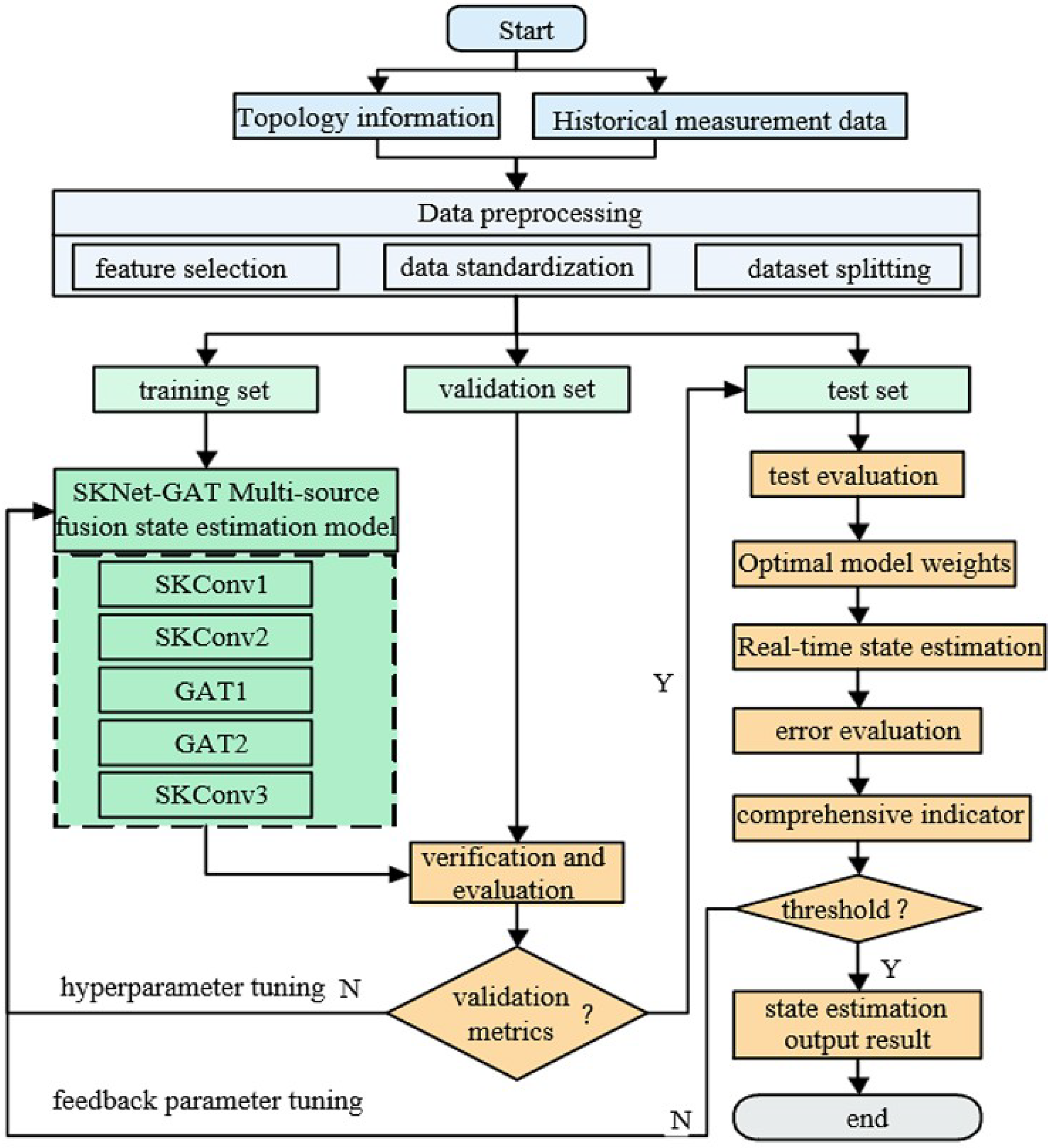
The optimization workflow of the proposed SKNet–GAT multi-source fusion state estimation model is illustrated in Figure 4.

(1)

Dataset preprocessing: The model input consists of two components: (i) the dynamic measurement vector derived from PMU and SCADA systems [29], including real-time measurements of nodal voltage magnitudes, phase angles, active/reactive power injections, and key branch flows, which comprehensively reflect the operational status; (ii) topological structure features, such as node degree, electrical distance, and switch status, describing the connectivity and potential topological switching of the network. After input layer normalization, these features form the initial feature vectors driving the SKNet–GAT state estimator.

To ensure consistency and mitigate the influence of differing scales, a min–max normalization is applied to each feature:

$${\overline{y}}_i={\displaystyle \frac{y_i-y_{min}}{y_{max}-y_{min}}}$$

(13)

where $y_i$ denotes the original feature value, $y_{min}$ and $y_{max}$ are the minimum and maximum values of the feature, and ${\tilde{y}}_i$ represents the normalized feature. This transformation preserves the relative differences while mitigating scale-induced biases during training. Finally, a 6:2:2 split is applied to the dataset for training, validation, and testing to support model learning, tuning, and generalization assessment.

(2)

Comprehensive evaluation metrics and error indicators: The performance of the proposed state estimator is evaluated using the root mean square error (RMSE), mean absolute error (MAE), and the coefficient of determination ($R^2$):

$${\mathrm{\Gamma }}_{\mathrm{RMSE}}=\sqrt{{\displaystyle \frac{1}{N}}{\sum }_{i=1}^N{\left(y_i-{\widehat{y}}_i\right)}^2},$$

(14)

$${\mathrm{\Gamma }}_{\mathrm{MAE}}={\displaystyle \frac{1}{N}}\sum _{i=1}^N\left|y_i-{\widehat{y}}_i\right|,$$

(15)

$$R^2=1-{\displaystyle \frac{{\sum }_{i=1}^N{\left(y_i-{\widehat{y}}_i\right)}^2}{{\sum }_{i=1}^N{\left(y_i-\overline{y}\right)}^2}},$$

(16)

where N is the total number of state variables, $y_i$ and ${\widehat{y}}_i$ denote the true and estimated values, respectively, and $\overline{y}$ is the mean of the true state values.

During training, although the standard Huber loss combines the benefits of MSE and MAE, its threshold parameter $\delta$ is typically fixed. To enhance convergence and robustness against outliers, we introduce an adaptive threshold Huber loss:

$${\zeta }_{\mathrm{Huber}}(y_i,{\widehat{y}}_i)=\left\{\begin{array}{cc}{\displaystyle \frac{1}{2}}{(y_i-{\widehat{y}}_i)}^2,\hfill & \mathrm{if}|y_i-{\widehat{y}}_i|\le {\delta }_t,\hfill \\ {\delta }_t\left(|y_i-{\widehat{y}}_i|-{\displaystyle \frac{1}{2}}{\delta }_t\right),\hfill & \mathrm{if}|y_i-{\widehat{y}}_i|>{\delta }_t.\hfill \end{array}\right.$$

(17)

where the adaptive threshold ${\delta }_t$ is defined as:

$${\delta }_t=\alpha ·\mathrm{Median}\left(|y_i-{\widehat{y}}_i|\right)+ϵ,$$

(18)

with $\alpha$ as an adjustment coefficient and $ϵ$ as a small smoothing term to prevent extremely small thresholds. This adaptive mechanism improves stability in early training while increasing robustness to outliers in later epochs.The model is optimized with Adam using an initial learning rate of 0.001, a batch size of 64, over 100 epochs.

The adaptive threshold ${\delta }_t$ overcomes a key limitation of standard Huber loss: a small fixed $\delta$ improves outlier robustness but slows early training, while a large fixed $\delta$ speeds convergence but weakens resistance to gross errors. In contrast, ${\delta }_t$ dynamically expands with large residuals in early epochs and narrows as residuals decrease in later epochs. This balance is essential for distribution network state estimation, where measurements contain both Gaussian noise and occasional outliers, eliminating the need for manual threshold tuning.For the detailed sensitivity analysis of $\alpha$ and the ablation study of the adaptive threshold mechanism, please refer to Section 4.2.4.

(3)

State estimation output: After training, the state estimation module outputs the voltage magnitude $\left|V\right|$ and phase angle $\theta$ for each node. The evaluation metrics (RMSE, MAE, $R^2$) are calculated to verify both accuracy and robustness, providing reliable inputs for subsequent dispatching and decision-making.

3.3. Multi-Source Feature Fusion and Multi-Scale Representation

To effectively capture the temporal dynamics and spatial dependencies of the distribution network, multi-source measurements from PMU and SCADA systems are fused and represented across multiple scales. Let the input measurement tensor be $\mathbf{X}\in {\mathbb{R}}^{T\times N\times C}$, where T is the temporal length. Multi-scale temporal features are first extracted via the Selective Kernel Convolution (SKConv) module [30]:

$$\mathbf{U}=\sum _{k=1}^K{\alpha }_k·{\varphi }_k\left({\mathbf{W}}_k\ast \mathbf{X}+{\mathbf{b}}_k+{\mathbf{\Gamma }}_k\odot \mathbf{X}\right),\sum _{k=1}^K{\alpha }_k=1,$$

(19)

where ∗ denotes convolution, $W_k$ and $b_k$ are kernel weights and bias; ${\mathrm{\Gamma }}_k\in {\mathbb{R}}^{T\times C}$ (one per kernel k) is a learnable modulation matrix that adaptively scales input feature channels via Hadamard product (⊙), emphasizing informative channels and suppressing noise for each scale; ${\varphi }_k(·)$ is a non-linear activation function; and ${\alpha }_k$ are adaptive gating weights obtained via global pooling and channel-wise attention.

Cross-source interactions are captured through a channel-wise attention mechanism with non-linear projection:

$${\mathbf{F}}_{i,j}=\sigma \left(\sum _{c=1}^C{\beta }_c·\mathrm{LayerNorm}({\mathbf{W}}_c{\mathbf{U}}_{:,i,c}+{\mathbf{b}}_c)+\psi \left({\mathbf{U}}_{:,i,c}\right)\right),\sum _{c=1}^C{\beta }_c=1,$$

(20)

where ${\mathbf{F}}_{i,j}$ is the fused feature for node i at time j, ${\beta }_c$ denotes the channel attention weight, ${\mathbf{W}}_c$ and ${\mathbf{b}}_c$ are linear projection parameters, $\mathrm{LayerNorm}(·)$ performs normalization, $\sigma (·)$ is a non-linear activation, and $\psi (·)$ is a learnable residual function enhancing representation power.

Spatial aggregation over the network is represented abstractly by a high-order graph aggregation operator:

$${\mathbf{G}}_i={\mathrm{\Phi }}_{\mathrm{GAT}}\left({\mathbf{F}}_i,\mathcal{A},\sum _{n=1}^N{\eta }_n{\mathbf{F}}_n{\mathbf{F}}_n^{\top },\mathrm{softmax}\left({\mathbf{a}}^{\top }[{\mathbf{F}}_i\Vert {\mathbf{F}}_n]\right)\right),$$

(21)

where ${\mathrm{\Phi }}_{\mathrm{GAT}}(·)$ represents the graph attention aggregation, $\mathcal{A}$ is the adjacency matrix, ${\eta }_n$ are node-wise learnable scaling factors, and the inner product ${\mathbf{F}}_n{\mathbf{F}}_n^{\top }$ captures high-order feature correlations between nodes.

Finally, the temporal and spatial features are fused to produce the final node embedding:

$${\mathbf{Z}}_i={\gamma }_1{\mathbf{G}}_i+{\gamma }_2{\mathbf{U}}_i+{\gamma }_{3}tanh({\mathbf{W}}_f[{\mathbf{G}}_i\Vert {\mathbf{U}}_i]+{\mathbf{b}}_f),{\gamma }_1+{\gamma }_2+{\gamma }_3=1,$$

(22)

where ${\mathbf{Z}}_i$ is the final embedding for node i, ${\gamma }_1,{\gamma }_2,{\gamma }_3$ are learnable fusion coefficients, ${\mathbf{W}}_f,{\mathbf{b}}_f$ are trainable projection parameters, and $tanh(·)$ adds non-linear fusion capability.

This multi-source, multi-scale representation forms the foundation for subsequent state estimation with physical consistency constraints, jointly considering temporal dynamics, heterogeneous measurement contributions, and electrical topology dependencies.

4. Case Study Analysis

4.1. Experimental Setup and Testing Systems

To evaluate the proposed SKNet–GAT method, two benchmark networks are used: the improved IEEE 33-node and IEEE 123-node systems [31], which provide realistic load distributions and topologies. Both systems are enhanced to reflect practical conditions: PMUs are installed at key nodes (3 for IEEE 33-node, 7 for IEEE 123-node) and SCADA sensors cover wide-area nodes with realistic noise; the IEEE 33-node system includes 30 modified topologies, and the IEEE 123-node system integrates 100 kW photovoltaic units and backup switches to simulate distributed generation and topological changes; random load perturbations (±10%) and Gaussian noise generate diverse samples. Detailed configurations are provided in Section 4.2 and Section 4.3. While Gaussian noise approximates measurement errors in this study, real-world data often contains non-Gaussian components and synchronization errors, which will be addressed in future field validations.

Implemented in Python with PyTorch 2.1.0 and Compute Unified Device Architecture (CUDA), the experiments run on a workstation equipped with a GeForce RTX 4060 GPU (8 GB) and CUDA Deep Neural Network Library (cuDNN) 11.8, with hyperparameters chosen through preliminary cross-validation.

Table 1. Experimental Setup and Benchmark System Specifications.

Property	IEEE 33-Node System	IEEE 123-Node System
Number of Nodes	33	123
Number of Branches	37	166
Voltage Level	12.66 kV	4.16 kV
Load Types	Constant/PQ Loads	Constant/PQ Loads + Distributed Generators
Topology Complexity	Radial	Radial with Loops
Computational Environment
Software	Python 3.10, PyTorch 2.1.0	Python 3.10, PyTorch 2.1.0
GPU	GeForce RTX 4060 (8 GB)	GeForce RTX 4060 (8 GB)
CUDA/cuDNN	CUDA 12.2/cuDNN 11.8	CUDA 12.2/cuDNN 11.8
AC Power Flow Simulation Toolbox	MATPOWER (v7.1)	MATPOWER (v7.1, Newton-Raphson solver)
Training Batch Size	64	64
Training Epochs	100	100
Learning Rate	0.001	0.001

summarizes the key characteristics of the benchmark systems and the computational environment.

This experimental setup ensures reproducibility and enables a fair comparison of the proposed method across networks of different sizes. By including both medium-scale and large-scale systems, the evaluation demonstrates the robustness, scalability, and generalization capability of the SKNet–GAT multi-source fusion approach under diverse operational scenarios.

To reflect real-world characteristics, the IEEE 33-node system is modified with PMU/SCADA deployment at specified nodes, 30 topology variants, and load-perturbed data; the IEEE 123-node system integrates 100 kW PV units, backup switching channels, and observability-optimized PMU placement. Both systems adopt realistic measurement noise and diverse data generation to validate the model’s robustness and scalability.

4.2. Improving IEEE 33 Node Distribution System Testing

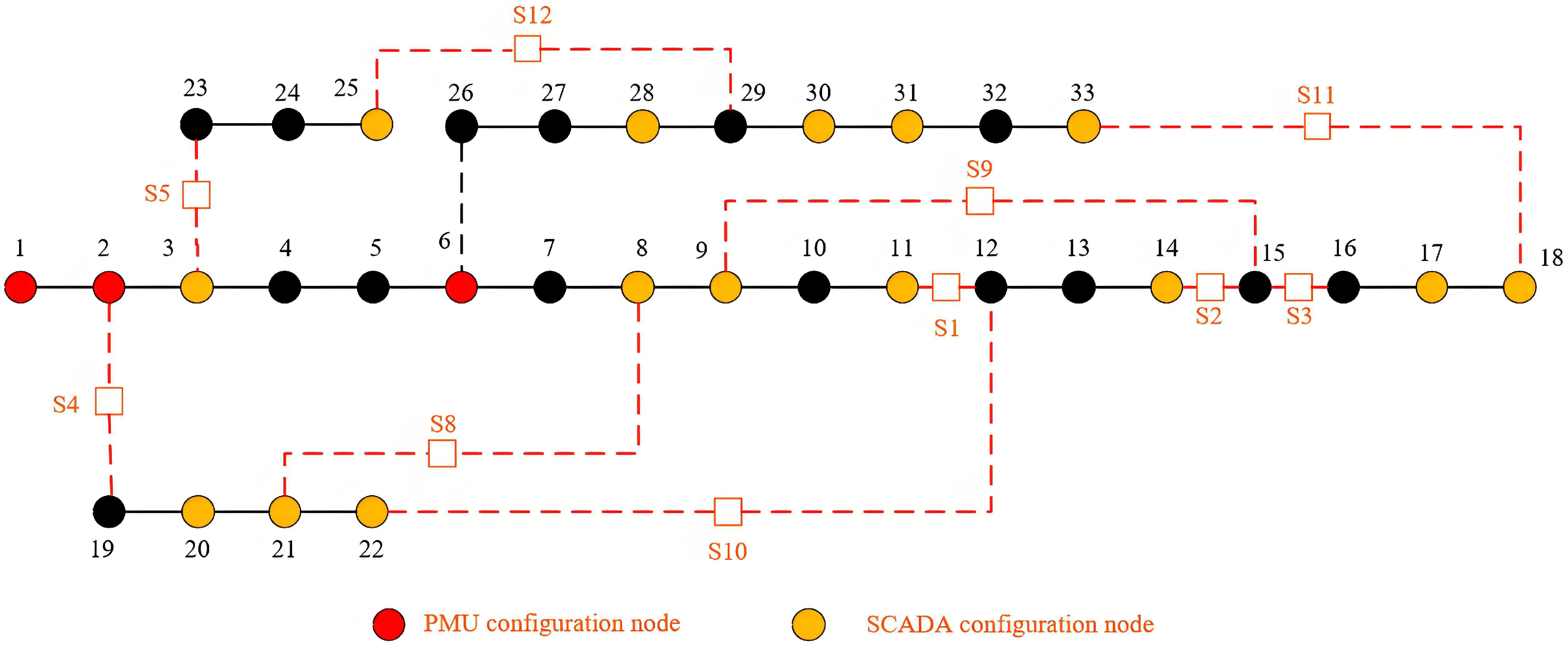
Adaptive modifications are made to the IEEE 33-bus system to better reflect real-world operational conditions, as shown in Figure 5. Considering the gradual deployment of PMUs in the distribution network and the widespread configuration of SCADA devices, this study chooses to install PMUs at nodes 1, 2, and 6 to collect node voltage amplitude and phase angle data. Measurement errors are modeled as Gaussian noise with mean zero, using a 0.15% standard deviation for voltage amplitude and 0.02° for phase angle. SCADA sensors at nodes 3, 8, 11, 15, 20, 24, and 28 monitor voltage amplitudes with a uniform 1% standard deviation.

Adaptive modifications are made to the IEEE 33-bus system to better reflect real-world operational conditions (Figure 5). PMUs are installed at nodes 1, 2, and 6 (voltage amplitude: $\sigma =0.15\%$ Gaussian noise; phase angle: $\sigma =0.{02}^{\circ }$ Gaussian noise), and SCADA sensors at nodes 3, 8, 11, 15, 20, 24, and 28 (voltage amplitude: $\sigma =1\%$ uniform noise). To test topology generalization, 30 modified topologies are generated by switching 1–3 breakers (maintaining radiality), with 300 dedicated test samples.

4.2.1. Data Generation and Sample Preparation

Based on the enhanced IEEE 33-node distribution network, the dataset for model training and evaluation is generated using historical load profiles and AC power flow simulations implemented in MATPOWER (a widely used open-source power system analysis toolbox). Typical weekday and weekend load curves from 2019 are selected as the primary data source, with a 15-min interval, yielding 3500 time series segments. An AC power flow simulation environment is constructed using MATPOWER’s runpf function, which solves the nonlinear power flow equations via the Newton-Raphson method. To increase sample diversity, random perturbations are applied to active and reactive loads at each node, including a uniform distribution factor in [0.9, 1.1] and a Gaussian noise component. AC power flow calculations in MATPOWER subsequently provide node voltage amplitudes, phase angles, active/reactive power injections, and branch power flows. All converged simulations are considered valid samples, resulting in approximately 6000 trend samples. All variables are then normalized using min-max scaling. A 6:2:2 split separates the data into training, validation, and test sets, offering a consistent and reproducible basis for model training, hyperparameter tuning, and performance evaluation.

To test the model’s topology generalization, additional test samples are generated based on modified network structures. Specifically, 30 new topologies are created by randomly switching 1–3 breakers in the original IEEE 33-node network, while maintaining radiality. The total load is preserved, and random perturbations are applied 10 times for each new topology. AC power flow solutions are then computed, generating a total of 300 samples for the topology generalization test set, which is kept separate.

Table 2. Data Generation and Sample Splitting.

Property	Trend Samples	Topology Generalization Samples
Network Base	IEEE 33-node	IEEE 33-node variants
Number of Topologies	1	30
Load Segments	3500	300
Perturbation Method	Uniform [0.9, 1.1] + Gaussian noise	Uniform [0.9, 1.1] + Gaussian noise
Power Flow	AC	AC
Converged Samples	6000	300
Normalization	Min–Max	Min–Max
Data Split (Train/Val/Test)	6:2:2	N/A (Test only)

summarizes the data generation process, sample sizes, and partitioning strategy.

4.2.2. Hyperparameter Optimization and Network Configuration

To fully leverage the capabilities of the SKNet–GAT model while ensuring convergence speed and generalization performance, Optuna Bayesian optimization is employed to tune key hyperparameters. After optimization, the following settings are adopted: AdamW with 0.001 learning rate, 32-sample batches, and 15% dropout uniformly applied to SKConv and GAT outputs. The maximum training duration is 200 epochs, using early stopping after 20 epochs of no validation improvement.The remaining key configurations are summarized in

Table 3. Key Hyperparameters of SKNet–GAT Model.

Parameter	Value
Input feature dimension	12
Time window step size	12
Hidden layer dimension	128
SKConv roll integral count	3
GAT layers/number of attention heads	2 layers/4 heads
Weight decay	$5\times {10}^{-4}$
Early stopping patience	20 epochs

.

For reproducibility and detailed reference,

Table 4. Hidden Layer Dimensions of SKNet–GAT Model.

Hidden Layer	Input Dimension	Output Dimension
Pro Conv	$(N,M,12,12)$	$(N,M,12,64)$
SKConv1	$(N,M,12,64)$	$(N,M,12,128)$
SKConv2	$(N,M,12,128)$	$(N,M,12,256)$
AvgPool-T	$(N,M,12,256)$	$(N,M,1,256)$
GAT-1	$(N,M,1,256)$	$(N,M,1,128)$
GAT-2	$(N,M,1,128)$	$(N,M,1,64)$
SKConv3	$(N,M,1,64)$	$(N,M,1,64)$
Fully Connected Layer	$(N,M,1,64)$	$(N,M,1,2)$

presents the input and output dimensions of each hidden layer during forward propagation. Here, $(N,M,T,C)$ denote batch size N, number of nodes M, time steps T, and feature channels C.

4.2.3. Model Hyperparameter Settings

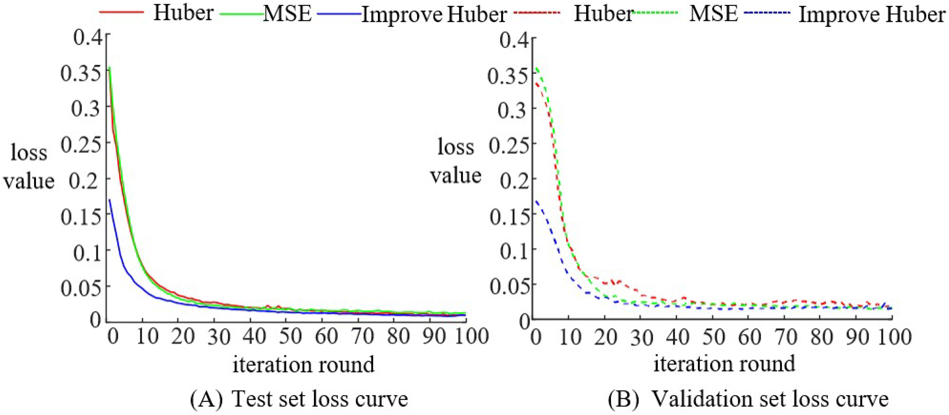
To visually assess the convergence and generalization of SKNet GAT on the IEEE 33-bus test system, Figure 6 presents the validation and test loss curves throughout training, comparing them with the conventional Huber and MSE losses to examine performance differences under different loss functions.

Figure 6A and Figure 6B, respectively, show the comparison of loss curves between the test set and the validation set under three different loss functions. It can be seen that the conventional Huber loss is relatively close to the MSE in terms of convergence speed and final convergence accuracy, with a rapid decrease in the early stage but a plateau in the middle and later stages, and the loss value remains at a relatively high level. The adaptive threshold Huber loss function proposed in this article can significantly reduce losses in the early stages of training and maintain a lower level than the benchmark method throughout the entire process, with faster convergence speed and significantly lower final convergence values. This indicates that the proposed loss function not only has stronger convergence during the optimization process but also demonstrates better generalization ability on the validation set, effectively improving the stability and accuracy of the SKNet GAT model in this system.

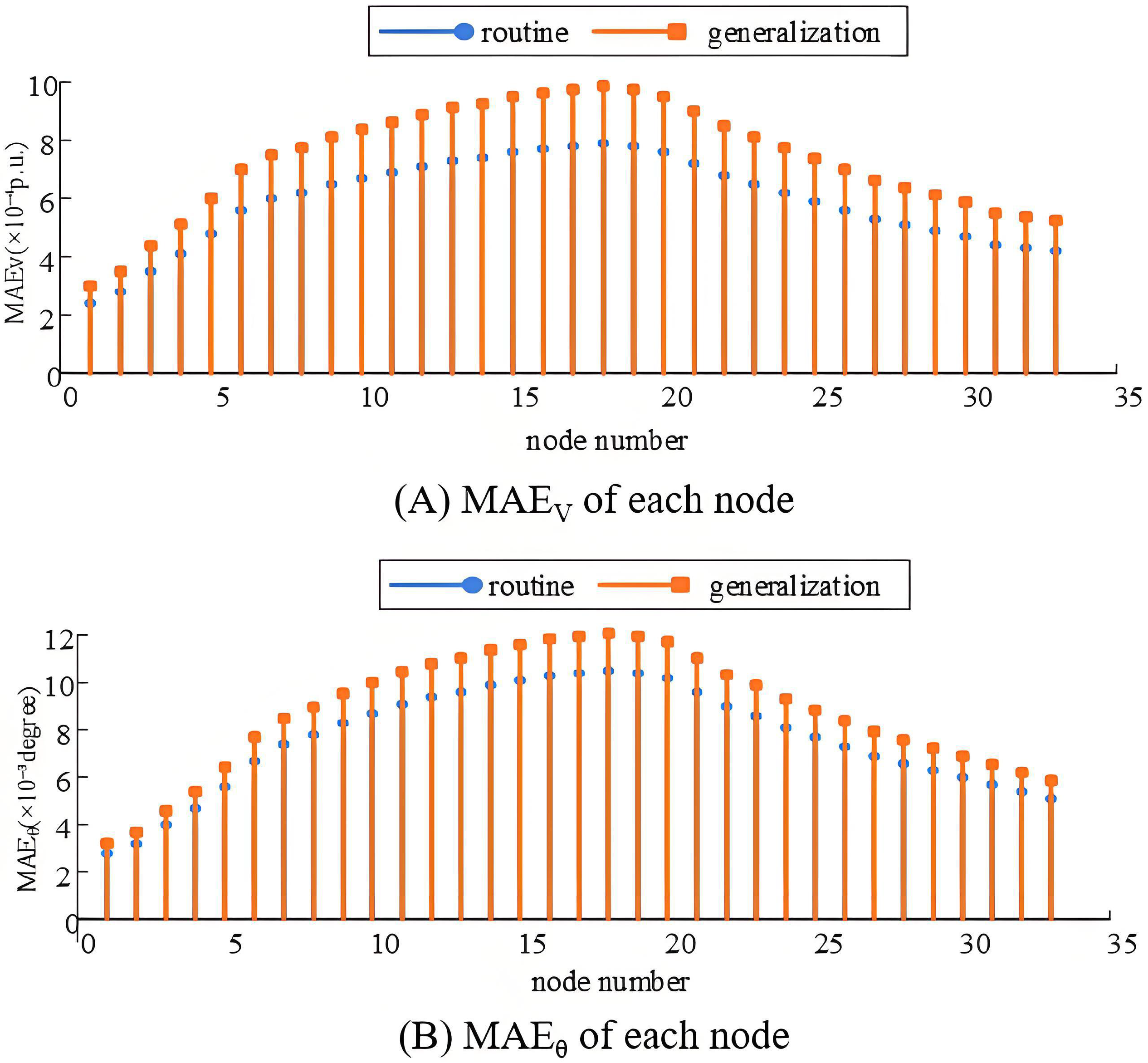
To visually compare the node-level estimation accuracy of SKNet GAT on the conventional test set and topology generalization test set, this section separately calculated the voltage amplitude ${\mathrm{MAE}}_V$ and phase angle ${\mathrm{MAE}}_{\theta }$ of 33 nodes, and plotted the error distribution of the two scenarios in the form of grouped bar charts, as shown in Figure 7.

From Figure 7, it can be observed that the node-level estimation error of the improved SKNet–GAT on the IEEE-33 node system exhibits an arched distribution pattern, being “slightly higher in the middle and lower at both ends.” Specifically, the voltage amplitude MAE ${\mathrm{MAE}}_V$ (Figure 7A) remains overall between $2\times {10}^{-4}\mathrm{p}.\mathrm{u}.$ and $1\times {10}^{-3}\mathrm{p}.\mathrm{u}.$, while the phase angle MAE ${\mathrm{MAE}}_{\theta }$ (Figure 7B) is controlled within the range $3\times {10}^{-3}$ to $1.2\times {10}^{-2}$, all far below the measurement noise level.

Compared to the conventional test set, in the topology generalization scenario, the error increases uniformly by only about 15–25%, and the curve shapes for each node remain almost identical, indicating that the model did not overfit to the training topology. The peak error is concentrated at nodes with high loads in the middle section of the feeder line, which is consistent with the expected pattern of “voltage gradually decreasing and noise amplification” in radial distribution networks. The findings confirm that the method achieves high accuracy and robustness despite unknown topologies and varying load conditions.

4.2.4. Sensitivity and Ablation Analysis of Adaptive Threshold

The adaptive threshold ${\delta }_t$ in the proposed Huber loss is a key factor determining both estimation accuracy and convergence behavior. To evaluate its influence, we conducted a sensitivity analysis of the adjustment coefficient $\alpha \in \{0.5,1.0,1.5,2.0,2.5,3.0\}$, while keeping other hyperparameters fixed (

Table 5. Sensitivity of Model Performance to $\alpha$.

$\mathit{\alpha }$	${\mathrm{MAE}}_{\mathit{V}}$ ($\times {10}^{-4}$ p.u.)	${\mathrm{MAE}}_{\mathit{\theta }}$ ($\times {10}^{-3}$)	Convergence Epoch
0.5	5.8	8.9	82
1.0	4.9	7.8	65
1.5	4.3	7.0	52
2.0	4.5	7.3	55
2.5	5.1	8.1	61
3.0	6.2	9.4	78

). The evaluation metrics include voltage amplitude MAE (${\mathrm{MAE}}_V$), phase angle MAE (${\mathrm{MAE}}_{\theta }$), and convergence epoch (number of epochs to reach validation loss $<{10}^{-4}$).

Table 5 shows that $\alpha =1.5$ achieves the best trade-off between accuracy and convergence. Smaller values ($\alpha <1.5$) over-constrain minor residuals, slowing convergence, while larger values ($\alpha >1.5$) reduce robustness to outliers. The stable range $\alpha \in [1.0,2.0]$ ensures flexibility for practical deployment.

We further validated the adaptive threshold through an ablation study, comparing it with fixed-threshold Huber losses ($\delta =0.1,0.3,0.5$) and standard MSE loss under the same test conditions (Gaussian noise with 20% outliers). The results are shown in

Table 6. Ablation Comparison of Loss Functions.

Loss Function	${\mathrm{MAE}}_{\mathit{V}}$ ($\times {10}^{-4}$ p.u.)	${\mathrm{MAE}}_{\mathit{\theta }}$ ($\times {10}^{-3}$)	Convergence Epoch
MSE	7.2	10.5	48
Fixed Huber ($\delta =0.1$)	6.5	9.8	72
Fixed Huber ($\delta =0.3$)	5.7	8.5	60
Fixed Huber ($\delta =0.5$)	6.1	9.2	55
Adaptive Huber ($\alpha =1.5$)	4.3	7.0	52

.

The adaptive Huber loss consistently outperforms fixed-threshold Huber and MSE losses in both accuracy and convergence, demonstrating the superiority of the adaptive threshold mechanism. Its effectiveness arises from the dynamic behavior of ${\delta }_t$: it expands during early epochs when residuals are large (favoring convergence, similar to MSE) and contracts as residuals decrease in later epochs (enhancing robustness to outliers, similar to MAE). This balance is essential in distribution network state estimation, where measurements often include Gaussian noise and occasional gross errors.

4.2.5. Comprehensive Performance Comparison

To comprehensively evaluate the advantages of SKNet–GAT across different technological routes, five representative baseline models were selected for horizontal comparison: the traditional optimization method WLS, the temporal depth model BiLSTM, its attention-enhanced variant BiLSTM-Att, the convolutional sequence fusion model SK-BiLSTM, and the state-of-the-art multi-scale graph attention network MS-GAT. All models were implemented on a unified IEEE-33 node dataset and trained under the same noise scenario, consisting of Gaussian noise ($\sigma =1\%/3\%/5\%$) combined with $\pm 20\%$ outliers, using a 6:2:2 train–validation–test split.

During testing, the voltage amplitude MAE $\left({\mathrm{MAE}}_V\right)$, phase angle MAE $\left({\mathrm{MAE}}_{\theta }\right)$, and single-section average inference latency were calculated to assess both accuracy and real-time performance.

Table 7. Comparison of State Estimation Accuracy and Inference Latency for Different Models.

Model	${\mathbf{MAE}}_{\mathit{V}}$	${\mathbf{RMSE}}_{\mathit{V}}$	${\mathit{R}}_{\mathit{V}}^2$	${\mathbf{MAE}}_{\mathit{\theta }}$	${\mathbf{RMSE}}_{\mathit{\theta }}$	${\mathit{R}}_{\mathit{\theta }}^2$	Latency (ms)
WLS	11.8	15.4	0.920	17.5	22.1	0.885	6
BiLSTM	8.4	10.7	0.954	12.0	15.5	0.929	32
BiLSTM-Attention	7.3	9.3	0.964	10.6	13.7	0.942	34
SK-BiLSTM	6.5	8.4	0.970	9.3	12.1	0.951	40
MS-GAT	5.1	6.7	0.984	7.9	10.4	0.966	48
SKNet-GAT	4.3	5.6	0.989	7.0	9.2	0.974	10

summarizes the results.

Table 7 shows that the traditional WLS method ranks lowest in all error metrics and $R^2$ values. The BiLSTM-based models significantly improve fitting performance (with $R^2$ increasing by approximately 4–6%), albeit at the cost of increased inference latency (>30 ms).

By incorporating multi-scale convolution and graph attention mechanisms (SK-BiLSTM and MS-GAT), both voltage and phase angle MAE/RMSE values decrease further, with $R^2$ exceeding 0.97. The proposed SKNet–GAT model achieves the best performance across five accuracy indicators: voltage MAE is only $4.3\times {10}^{-4}\mathrm{p}.\mathrm{u}.$, phase angle MAE is $7.0\times {10}^{-3}$, and $R^2$ reaches 0.989 and 0.974, respectively. Notably, its inference latency is only 10 ms, approaching the real-time level of WLS, demonstrating the model’s comprehensive superiority in accuracy, fitting, and computational efficiency.

Note that the reported inference latency (10 ms per section) only includes the model’s forward pass computation (from preprocessed feature input to estimation output) and excludes data preprocessing steps (e.g., normalization, time alignment), which are performed offline or in parallel in practical deployment.

4.3. Improving IEEE123 Node Distribution System Testing

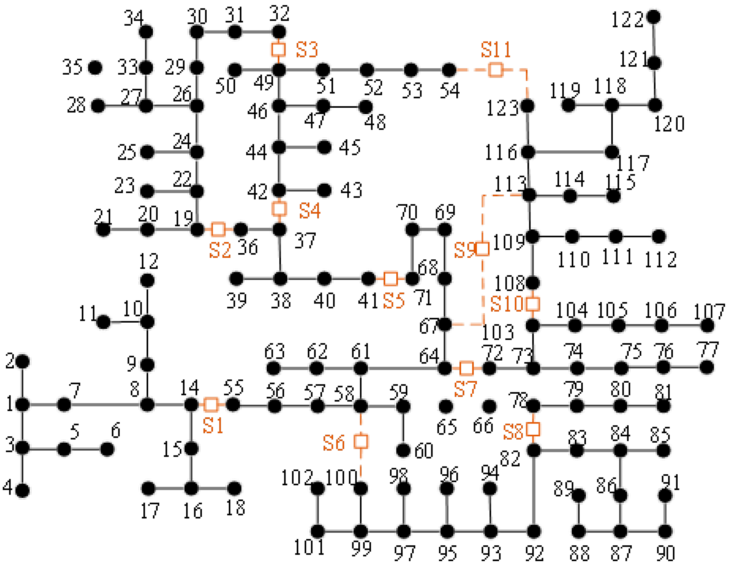
The improved IEEE 123-node distribution network testing system is illustrated in Figure 8. On the basis of the original feeder structure, the following improvements are introduced to simulate practical distribution network scenarios:

• Measurement configuration: Seven PMUs are installed at source busbar 1, backbone nodes 25, 46, 67, 79, 97, and the end node 123 to collect voltage amplitude and phase angle. PMU errors are modeled as zero-mean Gaussian with 0.15% standard deviation for amplitude and 0.02° for phase. SCADA devices are installed at high-load-density nodes to measure voltage, injected power, and branch flows with 1% measurement error.
• Distributed power generation and load variation: 100 kW photovoltaic units are connected to nodes 65, 83, and 114. Connection switches at nodes 38 and 98 are opened to form backup automatic switching channels.Node loads are randomly perturbed by ±10% following typical daily curves to simulate distributed energy fluctuations and load migration. AC power flow simulations for the improved IEEE 123-node system are also performed using MATPOWER, ensuring consistency with the IEEE 33-node system’s data generation pipeline. Observability verification: A PMU placement heuristic algorithm and topology constraints ensure full network observability, providing hierarchical redundancy along backbone branches.
• Observability verification: A PMU placement heuristic algorithm and topology constraints ensure full network observability, providing hierarchical redundancy along backbone branches.
• Measurement configuration: Seven PMUs are installed at the source busbar 1, backbone nodes 25, 46, 67, 79, 97, and end node 123 (same noise settings as the IEEE 33-node system), while SCADA devices are deployed at high-load-density nodes to monitor voltage, injected power, and branch flows (1% measurement error). Distributed generation and load variation are simulated by connecting 100 kW photovoltaic units at nodes 65, 83, and 114, and opening switches at nodes 38 and 98 to form backup automatic switching channels, with node loads perturbed by ±10% following typical daily curves. Observability is ensured using a PMU placement heuristic prioritizing backbone nodes for hierarchical redundancy.

To evaluate scalability, six models are migrated to the improved IEEE-123 node system and retrained under the unified protocol described in Section 3. Performance comparison of voltage and phase angle estimation, along with inference latency, is summarized in

Table 8. Performance Comparison of Various Models on the Improved IEEE-123 Node Distribution Network.

Model	${\mathbf{MAE}}_{\mathit{V}}$	${\mathbf{RMSE}}_{\mathit{V}}$	${\mathit{R}}_{\mathit{V}}^2$	${\mathbf{MAE}}_{\mathit{\theta }}$	${\mathbf{RMSE}}_{\mathit{\theta }}$	${\mathit{R}}_{\mathit{\theta }}^2$	Latency (ms)
WLS	18.7	24.0	0.905	28.5	35.0	0.860	12
BiLSTM	12.8	16.3	0.940	19.2	24.5	0.910	60
BiLSTM-Attention	11.0	14.1	0.952	16.7	21.5	0.925	64
SK-BiLSTM	9.9	12.7	0.962	14.9	19.1	0.936	75
MS-GAT	7.8	10.0	0.977	12.3	15.8	0.955	88
SKNet-GAT	6.4	8.2	0.983	11.1	14.3	0.965	18

. Consistent with the IEEE 33-node system’s latency definition, the reported 18 ms inference latency only reflects the model’s forward pass efficiency, excluding offline data preprocessing operations.

As shown in Table 8, when the network size increases from 33 to 123 nodes, all model errors increase, but the ranking remains consistent. Traditional WLS exhibits the largest voltage and phase angle MAE due to noise amplification. Deep time-series models (BiLSTM and BiLSTM-Attention) reduce errors by roughly 30% but suffer from inference latencies exceeding 60 ms. Multi-scale convolution and graph attention methods (SK-BiLSTM, MS-GAT) further improve accuracy with $R^2$ values ranging from 0.96 to 0.98, albeit at the cost of higher computational load. SKNet-GAT achieves the best overall performance, with voltage MAE of $6.4\times {10}^{-4}$ p.u., phase angle MAE of $11.1\times {10}^{-3}$, and an inference latency of only 18 ms, demonstrating excellent scalability and real-time capability.

Notably, SKNet-GAT’s 30% reduced parameter count and exploitation of distribution networks’ inherent sparsity enable scaling beyond the IEEE 123-node system. For networks with thousands of nodes, the sparse radial structure naturally limits the GAT’s attention calculation complexity, and additional optimizations (e.g., sparse attention implementations) can further mitigate potential memory challenges.

4.4. End-to-End Latency in Real-Time State Estimation

While SKNet-GAT demonstrates ultra-low inference latency (10–18 ms) for IEEE 33- and 123-node systems, practical deployment requires consideration of the end-to-end latency, which includes data transmission from PMU/SCADA devices, local edge preprocessing, and central computation. In industrial distribution networks, transmission latency depends on the communication medium (e.g., Ethernet, 5G, Wi-Fi) and can range from 2 to 20 ms. Edge preprocessing, such as local noise filtering, synchronization, and compression, typically adds 2–5 ms. Central computation, represented by the reported forward-pass latency, accounts for 10–18 ms depending on network size. Notably, the reported 10–18 ms excludes transmission and edge processing, which are critical in real-world scenarios.

In practice, asynchronous data generation from PMUs (50/60 Hz) and SCADA (1–5 min) requires time alignment, and wireless communication can introduce variable delays. For large-scale feeders with thousands of nodes, multi-hop transmission may accumulate latency. To mitigate these challenges, several strategies are proposed: integrating edge computing at measurement terminals to reduce transmission payload and local preprocessing delay; using low-latency communication protocols such as IEEE 1588 Precision Time Protocol (PTP) for synchronization and 5G URLLC for rapid transmission; and deploying hierarchical data aggregation via regional edge gateways to reduce multi-hop delays. These strategies can ensure end-to-end latency remains within 50–100 ms, supporting 1 s-level online monitoring.

Using these mitigation measures, a 1000-node distribution network is estimated to achieve an end-to-end latency of approximately 38 ms (5 ms transmission, 3 ms edge preprocessing, 30 ms central computation), well below typical industrial thresholds. Compared to conventional deep learning baselines, SKNet-GAT’s low computation latency provides additional flexibility to accommodate transmission variations, making it suitable for real-time monitoring and rapid operational decision-making. Future work will validate these estimates on Hardware-in-the-Loop platforms with real PMU/SCADA devices and 5G modules, and explore adaptive latency control mechanisms to enhance robustness under variable communication conditions.

5. Conclusions

An improved SKNet-GAT graph attention state estimator is proposed for multi-source measurement applications in power distribution systems. Systematic experimental verification is conducted on the improved IEEE-33 and IEEE-123 node systems, leading to the following conclusions:

• In both conventional and topology-generalization scenarios, the voltage amplitude and phase angle MAE of SKNet-GAT are reduced by approximately 65% and 60%, respectively, compared to the traditional WLS method, and further reduced by 15% and 12% relative to the best baseline model MS-GAT. Correspondingly, the voltage and phase angle $R^2$ values reach 0.989 and 0.974, demonstrating a significant improvement in the estimation accuracy for active distribution networks.
• Under Gaussian noise with $\sigma =1\%-5\%$, outliers of $\pm 20\%$, and 10% missing measurements, the estimation errors only increase uniformly by 15–25%, and the error curves remain consistent even under unknown topologies. This confirms the model’s robust adaptability to measurement noise, gross errors, and topological changes.
• Ultra-low inference latency: The proposed SKNet-GAT achieves an average latency of only 10 ms for the IEEE 33-node system and 18 ms for the IEEE 123-node system on a mid-range GeForce RTX 4060 (8GB) GPU. This measurement includes only the model’s forward pass and excludes offline preprocessing, making it approximately one-fifth the latency of deep learning baselines and comparable to the traditional WLS method (6 ms for IEEE 33-node).
• Practical deployment potential: Combined with a 30% reduction in total model parameters, this ultra-low latency enables direct deployment for 1 s-level online monitoring in large-scale distribution networks. It supports timely abnormal condition detection, rapid fault response, and real-time operational decision-making, highlighting a critical advantage over existing data-driven approaches that often trade speed for accuracy.

Despite these advantages, several limitations remain. First, the current evaluation relies entirely on MATPOWER-simulated data with Gaussian noise, which approximates measurement errors but cannot fully capture real-world characteristics such as non-Gaussian disturbances (e.g., impulsive noise from equipment faults) and PMU/SCADA synchronization errors. Second, for large-scale utility feeders with thousands of nodes, the GAT mechanism may face memory bottlenecks due to pairwise attention computation and feature aggregation. However, the sparse radial structure of distribution networks (average node degree $\approx 2$–3) and the model’s 30% reduced parameter count relative to baselines mitigate this concern. Third, performance under real-world operating conditions—including dynamic load variations, unmodeled distributed energy resources, and communication delays—requires further validation. Finally, the current framework focuses on steady-state estimation and does not yet incorporate dynamic state estimation or fault detection.

Future work will focus on three key directions: First, extending the SKNet-GAT framework to integrate real-time network measurements with Hardware-in-the-Loop (HIL) platforms for on-site validation, addressing non-Gaussian noise and synchronization errors in practical deployment; second, incorporating reinforcement learning (RL) to dynamically optimize model hyperparameters (e.g., GAT attention weights, SKNet kernel selection) based on real-time network conditions such as load volatility and topology changes, enabling adaptive performance under time-varying scenarios; and third, combining state estimation results with self-healing and adaptive control strategies to enhance distribution network resilience, reliability, and automation. Additionally, the practical benefits of ultra-low latency and reduced parameter count will be further explored to support real-time operational deployment.