Morris-Based Optimization of Battery Energy Storage System Control Parameters Under High Wind Energy Penetration

Abstract

As wind penetration rises, the share of synchronous generation declines, reducing system inertia and increasing uncertainty in frequency stability; wind-output disturbances, power-electronic control characteristics, and stochastic load variations can further amplify frequency deviations caused by power imbalance. To improve frequency security under high wind penetration, this study optimizes BESS control parameters and evaluates their impact on system dynamic stability using a PSS®E V34 dynamic model of the IEEE New England 39-bus system that includes three wind turbines and two BESS units under four disturbance scenarios: (i) derating one turbine to 50%, (ii) tripping one turbine, (iii) derating all three turbines to 50%, and (iv) an N-1 contingency corresponding to the tripping of the largest conventional generator in the system. Morris sensitivity analysis is first applied to identify key parameters affecting frequency response and reduce the optimization dimension, and the selected parameters are then tuned using an improved genetic algorithm (IGA) and grey wolf optimization (GWO). Simulation results show the minimum frequency improves from 59.957 Hz (baseline) to 59.961 Hz with IGA and to 59.966 Hz with GWO, while the maximum equivalent power-angle difference in the BESS unit relative to the center of inertia decreases from 266.3° to 250.1° (IGA) and 251.2° (GWO), indicating that the proposed approach strengthens BESS frequency support and enhances dynamic stability under various wind-power and N-1 contingency disturbance conditions.

1. Introduction

As the global energy mix accelerates its transition, the share of renewable energy in power grids continues to rise. Because its output is stochastic and intermittent, and because grid integration through power-electronic interfaces reduces the contribution of conventional rotational inertia, the system’s sensitivity to power imbalance and external disturbances increases significantly. Under high wind-penetration conditions, disturbance events can more easily trigger frequency deviations and may be accompanied by dynamic issues such as low-frequency oscillations, thereby increasing the risk to secure and stable grid operation [1,2].

Battery energy storage systems (BESSs) provide fast power regulation capability and strong controllability, and are therefore regarded as a key measure for supporting frequency regulation and damping oscillations [3,4]. However, in current engineering practice, controller parameters are often set to fixed values, making it difficult to accommodate changes in system topology, operating points, and disturbance types, which in turn limits regulation performance. To address this issue, recent studies have increasingly adopted evolutionary optimization and swarm-intelligence methods for controller parameter tuning [5,6,7,8]. Among them, genetic algorithms (GAs) can reduce the likelihood of becoming trapped in local optima through enhanced population diversity maintenance, adjusted crossover/mutation mechanisms, and fitness-guided strategies [9,10,11]. Grey wolf optimization (GWO), by contrast, employs hierarchical leadership and prey-encircling update rules to balance exploration and exploitation in the search process [12,13]. Compared with conventional genetic algorithms or other single heuristic strategies, IGA and GWO typically offer stronger global search capability, more robust convergence, and scalable computational procedures. Consequently, they are well suited to the multi-scenario requirements of BESS control-parameter optimization, delivering more effective frequency-support benefits under different disturbance conditions and operating states.

On the other hand, BESS control models usually include multiple layers of control loops and a large number of tunable parameters. Direct global optimization without prior screening can rapidly increase problem dimensionality, leading to substantially higher computational time and resource requirements and reducing practicality for large-scale systems. It is therefore necessary to first identify the key parameters that exert greater influence on system dynamics and frequency indices, and then optimize only this subset to reduce computational cost and improve solution efficiency. For this purpose, this study adopts Morris sensitivity analysis as a parameter-screening tool. By discretizing the parameter space and computing “elementary effects”, it evaluates both main effects and the impacts of nonlinearity and parameter interactions [14,15]. Recent studies have further demonstrated the effectiveness of the Morris method for efficient parameter screening and dimensionality reduction to support subsequent optimization [16,17]. In comparison, although Sobol sensitivity analysis provides a more comprehensive variance decomposition, it is computationally expensive [18], while the traditional one-at-a-time (OAT) approach is a local method that may underestimate interactions and bias importance ranking [19]. Overall, Morris offers a robust and computationally efficient means of ranking parameter importance, reducing optimization dimensionality, and improving the efficiency and reliability of subsequent IGA and GWO, while enabling the tuning process to focus on parameters that critically affect the frequency nadir and stable recovery.

Based on these considerations, this study proposes an integrated “Morris–IGA/GWO” framework. First, Morris sensitivity analysis is used to screen for highly influential parameters and to identify the control variables that are critical to frequency response and dynamic stability; then IGA and GWO are separately applied for parameter optimization, and the convergence characteristics and control effectiveness of the two algorithms are compared under multiple wind-disturbance scenarios. The results show that, relative to non-optimized BESS controller parameter settings, the optimized parameters more effectively suppress frequency drops and improve the system frequency nadir. Moreover, under the same test conditions, the solutions obtained by GWO exhibit overall superior performance to IGA in improving the frequency nadir, indicating stronger frequency-support capability and higher robustness. In summary, the proposed method aims to enhance the adaptability of BESS controllers across multiple operating points and disturbance conditions and to improve their frequency-support performance.

2. Study System Overview: Wind Turbine and Energy Storage Models

2.1. IEEE 39-Bus New England Power System

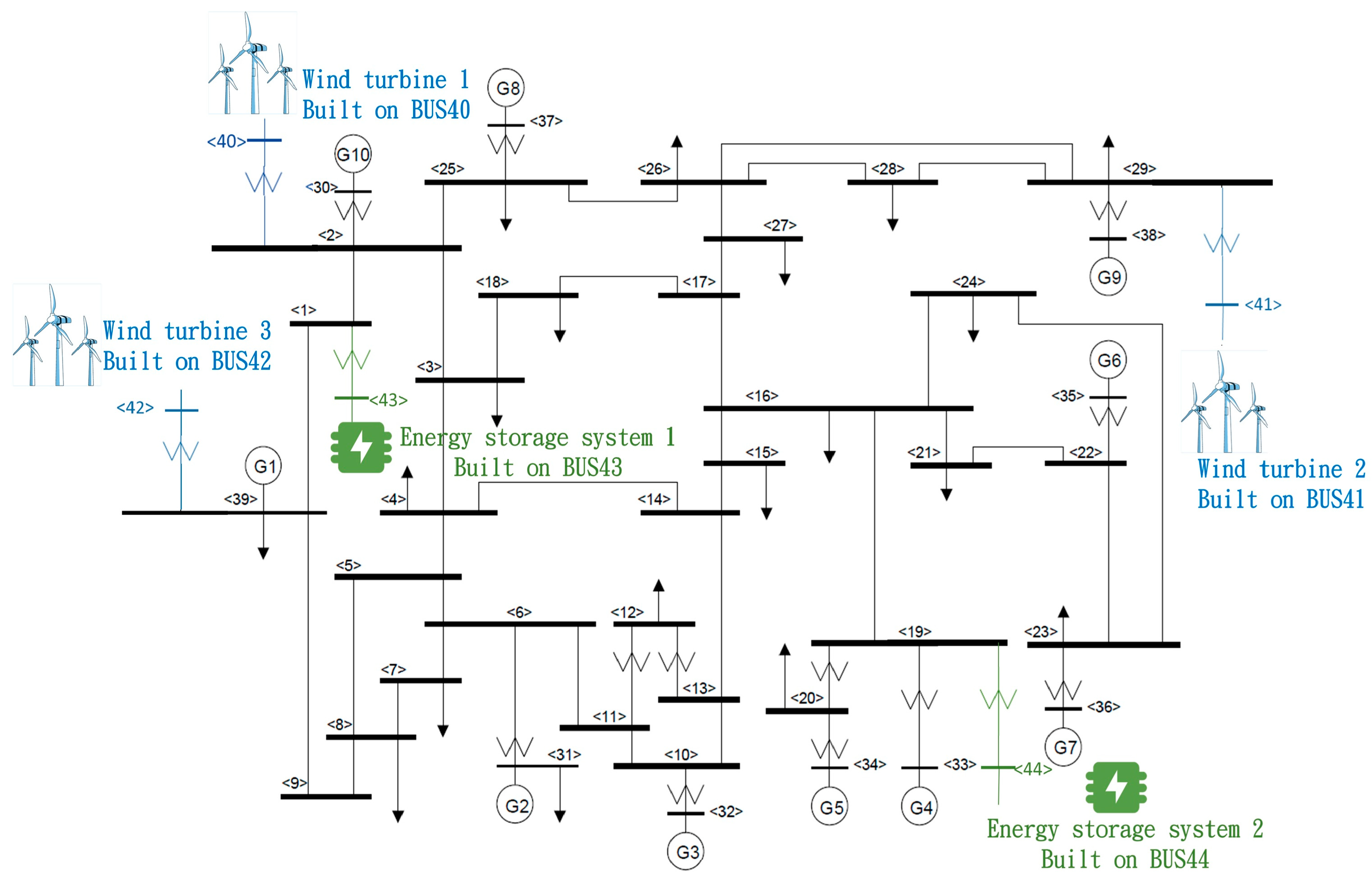
The IEEE 39-bus system (also known as the New England 10-machine system) is a widely used benchmark test network in power-system studies. Its original model is derived from an actual transmission system in the New England region of the United States and, after appropriate simplification and parameterization, has become a representative platform for analysis. The system consists of 39 buses, 10 synchronous generators, 46 transmission lines, and multiple transformers. With a clear topology and relatively complete data, it can reasonably reflect the typical operating characteristics and dynamic behavior of a medium-to-large power grid [20,21].

Accordingly, this model has been extensively applied in research on power-flow analysis, transient and small-signal stability assessment, as well as the validation of control strategies and the analysis of renewable-energy grid-integration impacts, as shown in Figure 1. Building on this benchmark, the present study further integrates three wind turbines and two battery energy storage systems (BESSs) to evaluate the system frequency response under high wind-penetration conditions.

2.2. Wind Turbine Model Structure

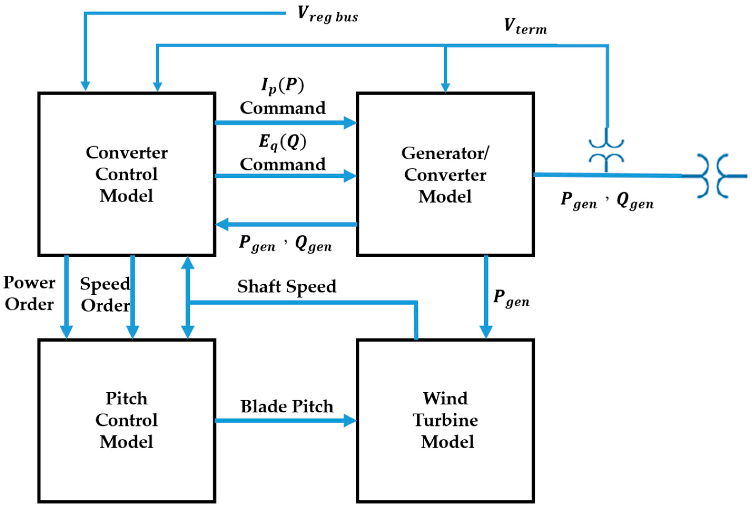
WT3 (WECC Type-3) is a widely used generic dynamic wind turbine generator model for representing the operating characteristics of DFIG-based wind turbines, and it is commonly implemented in power-system simulation software such as PSS^®E and PSLF. As shown in Figure 2 [22], its architecture is divided into four subsystems: the generator/converter plant, converter controls, the wind turbine rotor and drive train, and pitch control.

From a control perspective, WT3 regulates active and reactive power via current and voltage reference signals, respectively. Reactive power can be set by a fixed set-point or an external control signal, while active power is linked to rotor speed and operating/output conditions. The aerodynamic part is simplified, and pitch control uses a PI controller to correct speed and power errors. Due to its generic and simplified structure, WT3 is well suited for power-flow and dynamic studies of large-scale systems, and it is often used for aggregated wind-farm modeling to reduce complexity and computational burden.

2.3. Generic BESS Model Architecture

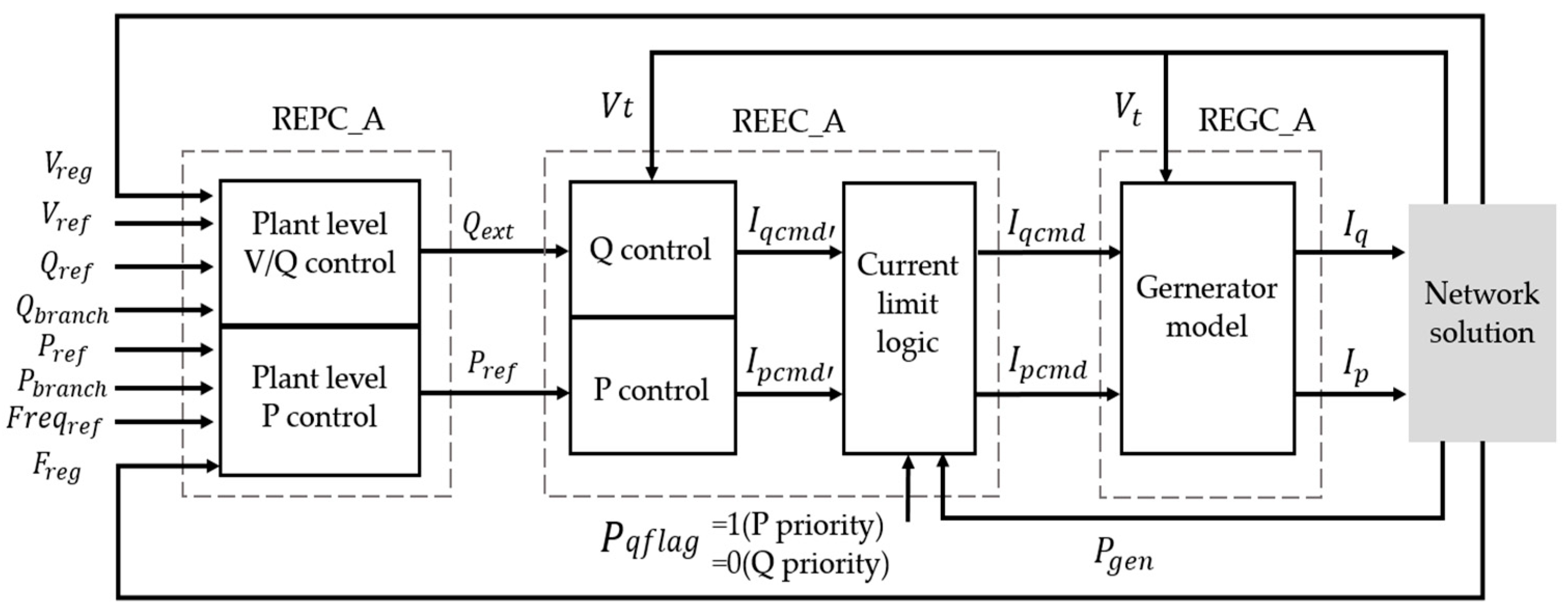
The BESS modeling and control framework used in this study follows the WECC second-generation generic model suite, where three modules—REPC, REGC, and REEC—are integrated to form a complete system (Figure 3). REPC provides supervisory control and generates commands by converting external requirements (e.g., active/reactive power or voltage/frequency support strategies) into power or current reference signals. REGC represents the grid-connected converter interface, translating reference signals and terminal voltage/current conditions into executable current commands while capturing the converter’s dynamic limits. REEC implements the detailed electrical control loops for voltage/reactive power and active power regulation, including output limits and protection functions, enabling fast and controllable support during disturbances [23].

This framework can also include state-of-charge (SOC) constraints to prevent the BESS from delivering power beyond its available energy, especially near charging/discharging boundaries. Overall, the modular design ensures consistency, portability, and comparability for system-level frequency and dynamic stability studies, and it allows control parameters to be adjusted across disturbance scenarios, forming the basis for Morris-based parameter screening and subsequent optimization using IGA/GWO.

2.4. Section Summary

This chapter presents the system and modeling framework used in this study. The IEEE 39-bus system is adopted as the test network, integrating three wind turbine generators and two BESS units under a high wind-penetration scenario. The wind turbines are modeled using the WECC Type-3 (WT3) generic model, including converter control, the generator/converter model, the rotor and drive train, and pitch control to capture the key dynamics of DFIG-based turbines. The BESS units employ the WECC second-generation generic framework, integrating REPC, REEC, and REGC to provide active/reactive power and voltage control while considering output limits. Overall, this chapter defines the study-system configuration and introduces the wind turbine and BESS models, forming the foundation for subsequent parameter screening and optimization analyses.

3. Morris Screening and IGA/GWO BESS Control Optimization Methods

3.1. Morris Sensitivity Analysis

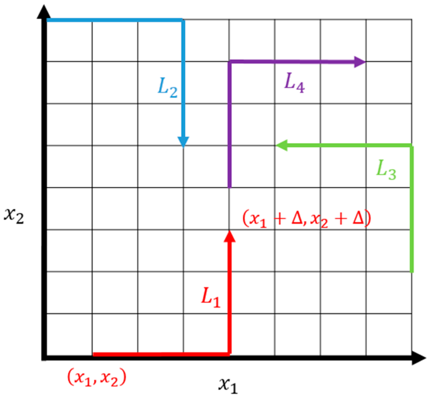
Morris is a global sensitivity analysis method developed for rapid screening of important parameters. It is based on the OAT (one-at-a-time) concept, where only one parameter is varied at a time. However, instead of evaluating sensitivity only near a single baseline point as in traditional OAT, Morris generates multiple random trajectories across the parameter space (Figure 4) and repeatedly applies one-parameter perturbations at different locations. This reduces dependence on the initial point and provides a distribution of each parameter’s influence.

By combining low computational cost with a global perspective, Morris is well suited for computationally expensive models with many parameters, where the goal is to identify key parameters for further detailed analysis or optimization [24,25].

In the Morris method, Equation (1) defines the elementary effect ($EE$) of the nth parameter: at a sampled input point x in the parameter space, only $x_n$ is increased by a step size $∆$ while all other parameters remain fixed, and sensitivity is quantified as the resulting change in model output divided by $∆$. Here, $N_p$ denotes the total number of parameters, and ${EE}_n$ represents the local strength of the output response to a perturbation in $x_n$ near that point; to avoid excessive dependence on any single sample, ${EE}_n$ is repeatedly computed along multiple random trajectories to obtain a more representative sensitivity assessment.

$${EE}_n={\displaystyle \frac{f\left(x_1,\dots ,x_{n-1},x_n+∆,\dots ,x_{N_p}\right)-f\left(x_1,\dots ,x_{n-1},x_n,\dots ,x_{N_p}\right)}{∆}}$$

(1)

In Equation (2), the elementary effects (EEs) obtained from each randomized trajectory are first taken in absolute value and then averaged to yield ${\mathsf{\mu }}_n^{\ast }$, which represents the overall influence of the nth parameter on the model output. Here, $L$ denotes the number of randomized trajectories (or repeated samplings), and ${EE}_n^{\left(\mathcal{l}\right)}$ is the elementary effect of the nth parameter along the $\mathcal{l}$th trajectory. A larger ${\mathsf{\mu }}_n^{\ast }$ therefore indicates a more influential (i.e., more important) parameter. Next, Equation (3) computes the variance (or equivalently, the standard deviation) of the EEs, ${\mathsf{\sigma }}_n^2$, to quantify how much the elementary effects fluctuate across different sampling locations. In this equation, ${\mathsf{\mu }}_n$ is the mean of the EEs without taking absolute values, and $L-1$ is the degrees-of-freedom correction term used in the sample-variance calculation. A relatively large ${\mathsf{\sigma }}_n^2$ (or ${\mathsf{\sigma }}_n$) typically implies that the parameter’s effect varies substantially with the sampling location, suggesting potential nonlinear behavior or interactions with other parameters.

$${\mathsf{\mu }}_n^{\ast }={\displaystyle \frac{1}{L}}\sum _{\mathcal{l}=1}^L\left|{EE}_n^{\left(\mathcal{l}\right)}\right|$$

(2)

$${\mathsf{\sigma }}_n^2={\displaystyle \frac{1}{L-1}}\sum _{\mathcal{l}=1}^L{({EE}_n^{\left(\mathcal{l}\right)}-{\mathsf{\mu }}_n)}^2$$

(3)

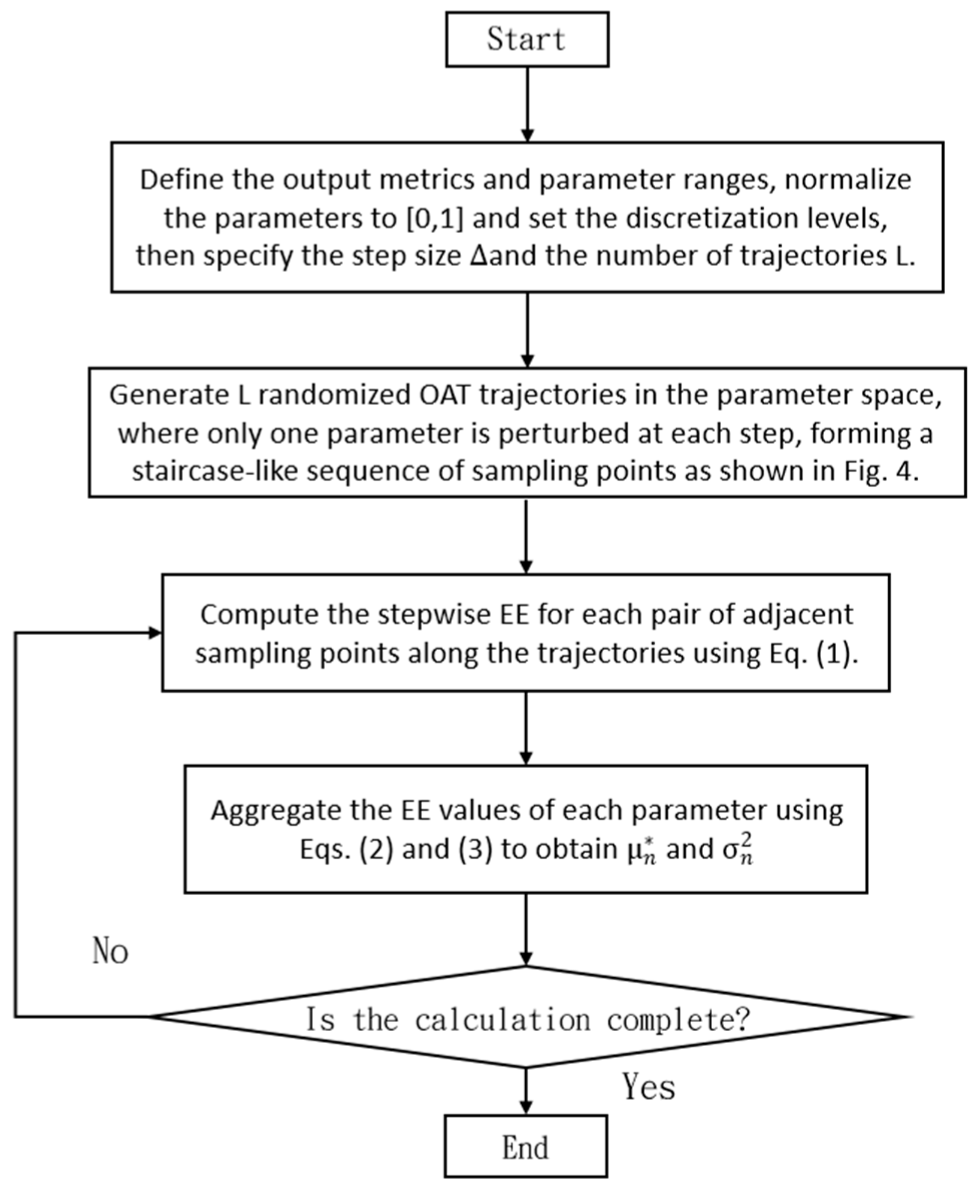
By jointly considering ${\mathsf{\mu }}_n^{\ast }$ and ${\mathsf{\sigma }}_n^2$, parameters can be further classified into those with negligible influence, those exhibiting approximately linear and additive effects, and those showing nonlinear effects and/or interactions [26,27]. The overall procedure of the Morris sensitivity analysis is illustrated in Figure 5.

3.2. Improved Genetic Algorithm

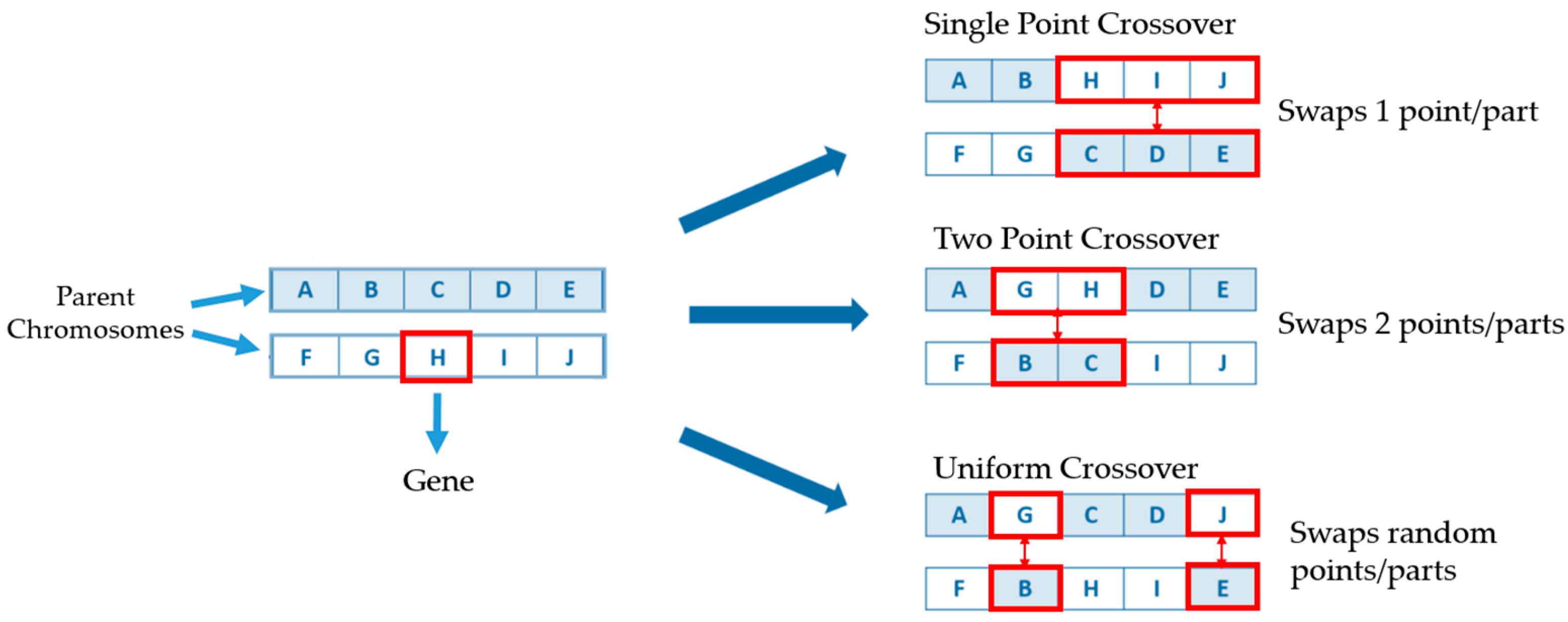
Genetic algorithms (GAs) are probabilistic optimization methods inspired by biological evolution, based on the principle of “survival of the fittest.” Instead of following a single search path, a GA maintains a population of candidate solutions (individuals), with decision variables encoded as chromosomes. Through evolutionary operators—selection, crossover, and mutation—better individuals are more likely to be retained and to pass their traits to the next generation [28,29]. Crossover recombines gene segments from two parents to produce offspring solutions (Figure 6) [30], while mutation introduces small random changes to maintain diversity and reduce the risk of local optima. The population is iteratively updated until a stopping criterion is met (e.g., reaching the maximum generations or no further improvement). GAs are relatively insensitive to initial conditions and are suitable for nonlinear or discrete problems, but their stochastic nature means they do not guarantee a true global optimum.

Although a conventional genetic algorithm (GA) can search using a population in parallel, it still has several limitations: it cannot guarantee a global optimum and may suffer from premature convergence; moreover, its performance is highly sensitive to parameter settings, and inappropriate choices can lead to slow convergence or unstable solutions. To improve the search efficiency of GA in a continuous-parameter space, this study adopts the improved GA framework in [31], incorporating a “survival of the fittest” mechanism into the traditional workflow and employing a multi-offspring arithmetic crossover scheme. Specifically, the population is first ranked by fitness, and elite individuals are selected as parents. Then, four different offspring are generated simultaneously using weighted combinations defined in Equations (4)–(9), which enhances diversity and reduces the risk of being trapped in local optima.

Here, in Equation (4), ${\mathrm{b}}_1$ is the average of the parent vectors $a_s$ and $a_t$. In Equations (5) and (6) ${\mathrm{b}}_2$ and ${\mathrm{b}}_3$ incorporate the weight $\omega$ together with $a_{max}$ and $a_{min}$, such that the offspring are extrapolated toward the upper bound and the lower bound, respectively. The operators $\mathrm{m}\mathrm{a}\mathrm{x}(a_s,a_t)$ and $\mathrm{m}\mathrm{i}\mathrm{n}(a_s,a_t)$ denote, in each dimension, the element-wise maximum and element-wise minimum of the two parent vectors. Equation (7) further combines the element-wise maxima/minima with the parental average. In Equations (8) and (9), $a_{max}$ and $a_{min}$ represent the upper and lower bounds of the design variables in each dimension.

$${\mathrm{b}}_1=\left[b_1^1,b_2^1,\dots ,b_n^1\right]={\displaystyle \frac{a_s+a_t}{2}}$$

(4)

$${\mathrm{b}}_2=\left[b_1^2,b_2^2,\dots ,b_n^2\right]=a_{max}\left(1-\omega \right)+\mathrm{m}\mathrm{a}\mathrm{x}(a_s,a_t)\omega$$

(5)

$${\mathrm{b}}_3=\left[b_1^3,b_2^3,\dots ,b_n^3\right]=a_{min}\left(1-\omega \right)+\mathrm{m}\mathrm{i}\mathrm{n}(a_s,a_t)\omega$$

(6)

$${\mathrm{b}}_4=\left[b_1^4,b_2^4,\dots ,b_n^4\right]={\displaystyle \frac{\left(a_{max}+a_{min}\right)\left(1-\omega \right)+(a_s+a_t)\omega }{2}}$$

(7)

$$a_{max}=\left[x_1^{max},x_2^{max},\dots ,x_n^{max}\right]$$

(8)

$$a_{min}=\left[x_1^{min},x_2^{min},\dots ,x_n^{min}\right]$$

(9)

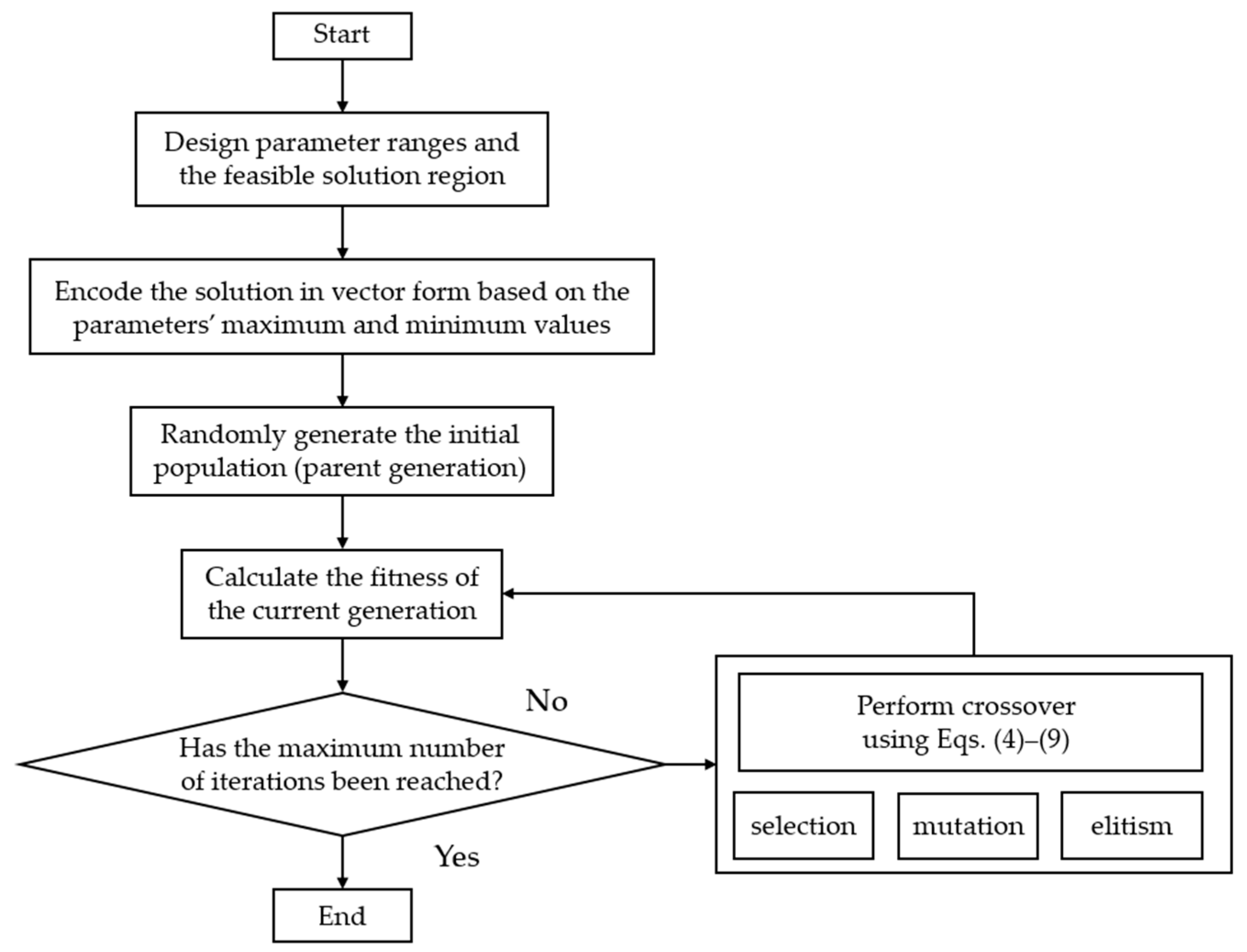
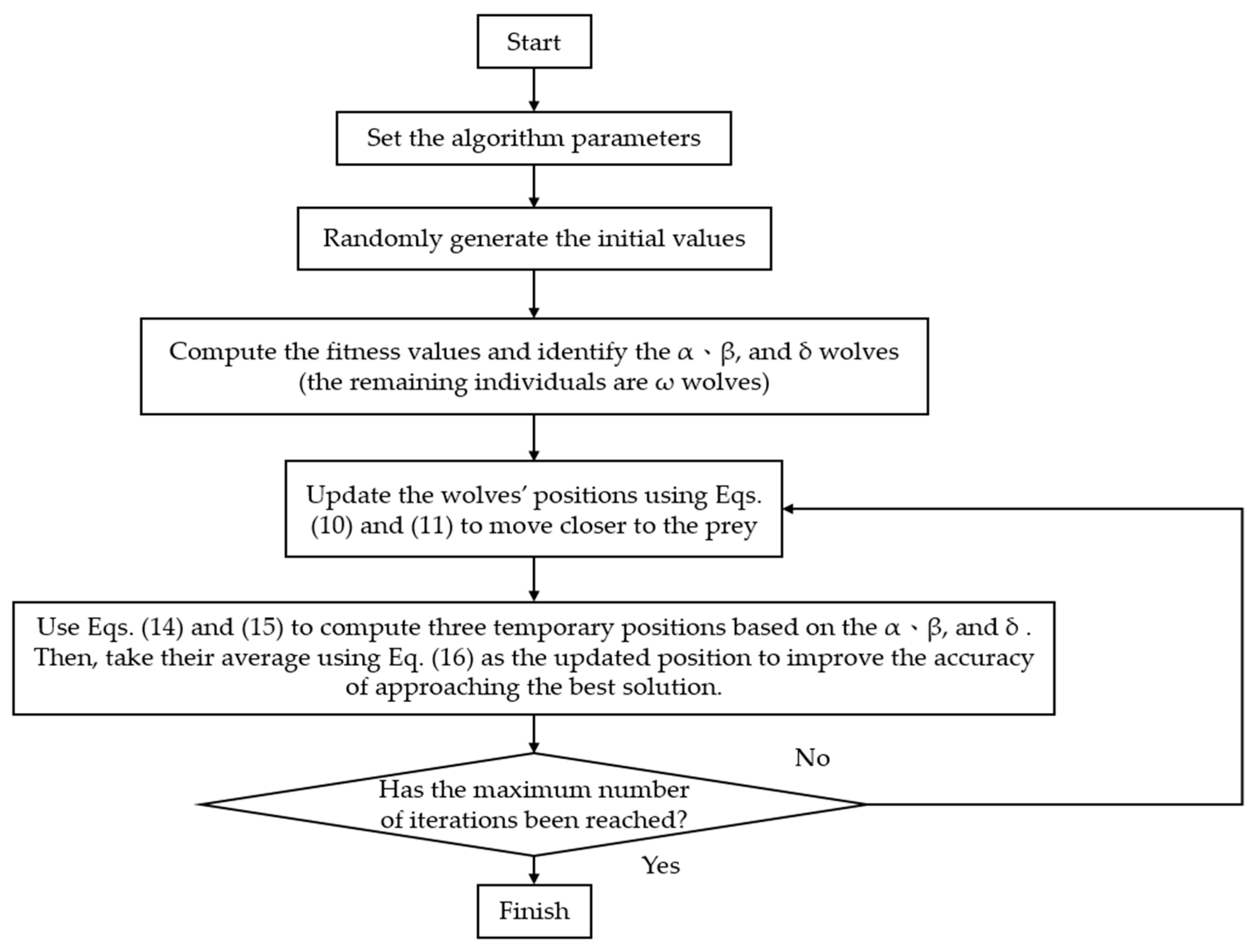
The flowchart of the IGA is shown in Figure 7.

3.3. Grey Wolf Optimization

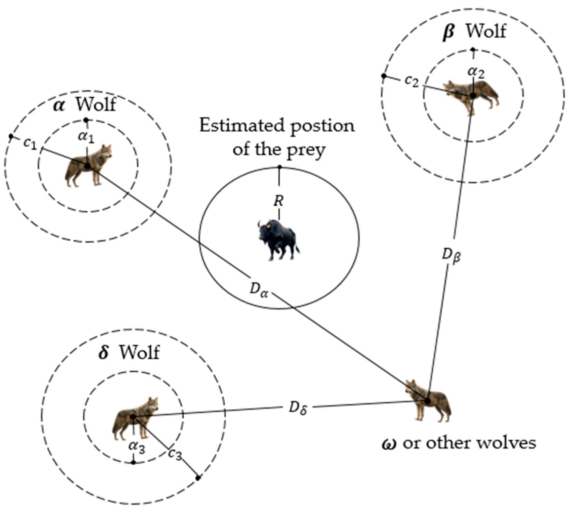
Grey Wolf Optimization (GWO) is a swarm-intelligence optimization method that mimics the social hierarchy and hunting (encircling) behavior of grey wolves. In this algorithm, the three best solutions in the population are regarded as the leaders α, β, and δ, while the remaining individuals are denoted as ω. At each iteration, the ω wolves update their positions under the guidance of α, β, and δ, enabling the population to progressively move toward better solutions [32,33]. As illustrated in Figure 8, α, β, and δ provide guidance toward the estimated prey position and form three corresponding distance vectors $D_{\alpha }$, $D_{\mathsf{\beta }}$, and $D_{\mathsf{\delta }}$. The ω\omega ω wolves then adjust their movement direction and step size under the combined influence of these leaders, which is equivalent to multiple leaders jointly “encircling” the target and gradually shrinking the search region. Accordingly, GWO transitions from strong exploration in the early stage to increasingly intensified exploitation in the later stage, converging from coarse to fine toward the vicinity of the optimal solution in the search space.

In Grey Wolf Optimization (GWO), the position update of each individual is formulated based on the concept of “encircling the prey.” First, Equation (10) is used to compute the distance vector between a grey wolf and the prey, where $t$ denotes the iteration index, $\overrightarrow{\mathrm{X}}\left(\mathrm{t}\right)$ is the current position of the grey wolf, and $\overrightarrow{X_p}$(t) is the estimated position of the prey (i.e., the target). Next, Equation (11) updates the position so that the individual moves toward the target under the regulation of the coefficient vector $\overrightarrow{\mathrm{A}}$.

$$\overrightarrow{\mathrm{D}}=|\overrightarrow{\mathrm{C}}\times \overrightarrow{X_p}(\mathrm{t})-\overrightarrow{\mathrm{X}}\left(\mathrm{t}\right)|$$

(10)

$$\overrightarrow{\mathrm{X}}\left(t+1\right)=\overrightarrow{X_p}(\mathrm{t})-\overrightarrow{\mathrm{A}}\times \overrightarrow{\mathrm{D}}$$

(11)

The coefficient vectors $\overrightarrow{\mathrm{A}}$ and $\overrightarrow{\mathrm{C}}$ are defined by Equations (12) and (13), respectively, where $r_1$ and $r_2$ are random vectors in the range [0, 1]. The parameter $\overrightarrow{a}$ decreases linearly from 2 to 0 over the course of iterations, thereby adjusting the balance between exploration and exploitation.

$$\overrightarrow{\mathrm{A}}=2\overrightarrow{a}\times \overrightarrow{r_1}-\overrightarrow{a}$$

(12)

$$\overrightarrow{\mathrm{C}}=2\times \overrightarrow{r_2}$$

(13)

During the hunting phase, GWO uses the three leaders α, β, and δ simultaneously as guidance sources. First, Equation (14) is applied to compute $\overrightarrow{D_{\mathsf{\alpha }}}$, $\overrightarrow{D_{\mathsf{\beta }}}$, and $\overrightarrow{D_{\mathsf{\delta }}}$, and then Equation (15) is used to obtain three intermediate positions, $\overrightarrow{X_1}$, $\overrightarrow{X_2}$, and $\overrightarrow{X_3}$. Finally, Equation (16) takes the average of these three positions as the individual’s new location. This is equivalent to having each grey wolf be jointly pulled by the three best solutions, which improves update stability and reduces the risk of being trapped in local optima [34,35].

$$\begin{array}{c}\overrightarrow{D_{\mathsf{\alpha }}}=\left|\overrightarrow{C_1}\times \overrightarrow{X_{\mathsf{\alpha }}}-\overrightarrow{X}\right|\\ \overrightarrow{D_{\mathsf{\beta }}}=\left|\overrightarrow{C_2}\times \overrightarrow{X_{\mathsf{\beta }}}-\overrightarrow{X}\right|\\ \overrightarrow{D_{\mathsf{\delta }}}=\left|\overrightarrow{C_3}\times \overrightarrow{X_{\mathsf{\delta }}}-\overrightarrow{X}\right|\end{array}$$

(14)

$$\begin{array}{c}\overrightarrow{X_1}=\overrightarrow{X_{\mathsf{\alpha }}}-\overrightarrow{A_1}\times \left(\overrightarrow{D_{\mathsf{\alpha }}}\right)\\ \overrightarrow{X_2}=\overrightarrow{X_{\mathsf{\beta }}}-\overrightarrow{A_2}\times \left(\overrightarrow{D_{\mathsf{\beta }}}\right)\\ \overrightarrow{X_3}=\overrightarrow{X_{\mathsf{\delta }}}-\overrightarrow{A_3}\times \left(\overrightarrow{D_{\mathsf{\delta }}}\right)\end{array}$$

(15)

$$\overrightarrow{\mathrm{X}}\left(t+1\right)={\displaystyle \frac{\overrightarrow{X_1}+\overrightarrow{X_2}+\overrightarrow{X_3}}{3}}$$

(16)

The flowchart of the GWO is shown in Figure 9.

3.4. Objective Function

In this study, the post-disturbance frequency response of the system is used as the basis for performance evaluation. Five frequency performance indices are selected to quantify frequency nadir, recovery characteristics, and steady-state oscillatory behavior: the minimum frequency $f_{min}$, the frequency at the end of simulation $f_{end}$, the standard deviation of frequency in the steady-state interval $f_{steady}$, the steady-state frequency fluctuation range ${Range}_{steady}$, and the number of post-steady-state oscillations (Oscillations). The definitions and calculation methods of these indices are given in Equations (17)–(23) [36].

Equation (17) extracts the minimum frequency $f_{min}$ after a disturbance to quantify the frequency nadir. Since the nadir reflects the frequency security margin and potential under-frequency protection/load-shedding risk, $f_{min}$ is defined as the minimum value of the simulated frequency trajectory. A higher $f_{min}$ indicates a smaller frequency dip and stronger frequency support under different controller parameter settings.

$$f_{min}=\mathrm{m}\mathrm{i}\mathrm{n}(f_1,f_2,\cdots ,f_n)$$

(17)

Equation (18) defines the end-of-simulation frequency $f_{end}$ to assess the final recovery level after a disturbance and the resulting steady-state deviation from the nominal value. In this study, $f_{end}$ is taken as the last frequency sample in the time series, where $f_n$ is the frequency at the nth (final) sampling point and $n$ is the total number of samples.

$$f_{end}=f_n$$

(18)

Equations (19)–(23) quantify post-steady-state frequency oscillations (steady state defined as $t_i$ > 10 s) from three aspects: dispersion, fluctuation magnitude, and oscillation count. Equation (19) computes the steady-state mean $\mu$; Equation (20) computes the steady-state standard deviation $f_{steady}$ relative to $\mu$; Equation (21) defines ${Range}_{steady}$ as the max–min frequency in the steady-state interval. Equations (22)–(23) count crossings $N_{cross}$ based on sign changes in consecutive samples relative to $\mu$ and estimate the oscillation count (Oscillations). Here, $t_i$ and $f_i$ are the time and frequency of the ith sample, and m is the number of samples with $t_i>10$.

$$\mu ={\displaystyle \frac{1}{m}}\sum _{i=1}^m{f}_i,for{t}_i>10$$

(19)

$$f_{steady}=\sqrt[]{{\displaystyle \frac{1}{m}}\sum _{i=1}^m{\left(f_i-\mu \right)}^2},for{t}_i>10$$

(20)

$${Range}_{steady}=\max \left(f_i\right)-\min \left(f_i\right),for{t}_i>10$$

(21)

$$N_{cross}=\left(f_{i-1}-\mu \right)\times \left(f_i-\mu \right)<0$$

(22)

$$\mathrm{O}\mathrm{s}\mathrm{c}\mathrm{i}\mathrm{l}\mathrm{l}\mathrm{a}\mathrm{t}\mathrm{i}\mathrm{o}\mathrm{n}\mathrm{s}=⌊{\displaystyle \frac{N_{cross}}{2}}⌋$$

(23)

Equations (24)–(29) normalize the five frequency indices into dimensionless values ($Norm$) to remove unit/scale effects and prevent any single metric from dominating the objective function. Equation (29) then combines the normalized metrics into an overall weighted score ($Score$), which is used as the objective function in IGA and GWO; a higher score indicates better overall frequency performance.

Since the main goal is to suppress post-disturbance frequency drops and improve recovery, the minimum and terminal frequencies are assigned the highest (W₁) and second-highest (W₂) weights. The remaining metrics capture steady-state quality and damping and thus receive lower weights to balance short-term support and longer-term stability. The specific values of W₁–W₅ are listed in

Table 1. Weights and definitions of W₁–W₅.

Parameter	Denotation	Value
$W_1$	Weight for minimum frequency	0.375
$W_2$	Weight of steady-state frequency standard deviation	0.125
$W_3$	Weight of frequency at the end of simulation	0.208
$W_4$	Weight of steady-state frequency fluctuation range	0.125
$W_5$	Weight of number of post-steady-state oscillations	0.167

.

$${Norm}_{min}={\displaystyle \frac{1}{1+e^{-200(f_{min}-59.957)}}}$$

(24)

$${Norm}_{f_{\mathrm{steady}}}={\displaystyle \frac{1}{1+60\times f_{\mathrm{steady}}}}$$

(25)

$${Norm}_{end}=e^{-{({\displaystyle \frac{|f_{end}-60|}{0.01}})}^2}$$

(26)

$${Norm}_{range}={\displaystyle \frac{1}{1+1000\times {Range}_{steady}}}$$

(27)

$${Norm}_{osc}={\displaystyle \frac{1}{1+0.6\times \mathrm{Oscillations}}}$$

(28)

$$Score=W_1\ast {Norm}_{min}+W_2\ast {Norm}_{f_{\mathrm{steady}}}+W_3\ast {Norm}_{end}+W_4\ast {Norm}_{range}+W_5\ast {Norm}_{osc}$$

(29)

4. Research Results

4.1. Overall Research Procedure

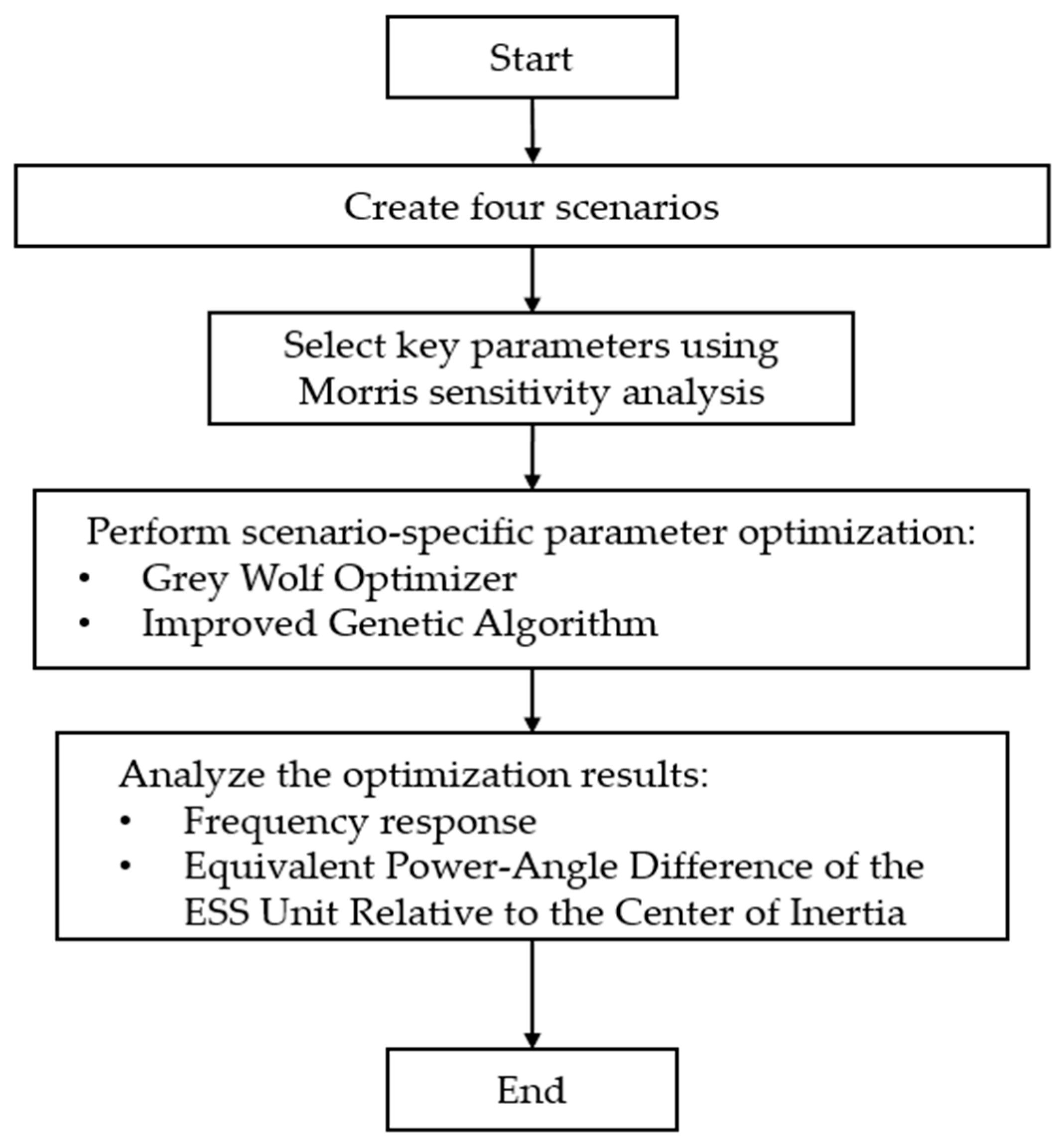
The experimental workflow is shown in Figure 10. First, three wind power output scenarios are defined to represent different operating conditions. Next, Morris sensitivity analysis is used to identify key parameters affecting the frequency response, thereby reducing the optimization dimension and computational cost. Then, for each scenario, GWO and IGA are applied to search for the optimal parameter set. Finally, frequency responses and rotor angle separations are compared across scenarios to assess improvements in frequency performance and transient stability.

4.2. Wind Turbine Scenario Setup

Four disturbance scenarios are considered: (1) one wind turbine reduced to half load, (2) one wind turbine tripped, (3) three wind turbines reduced to half load, and (4) an N-1 contingency corresponding to the tripping of the largest conventional generator in the system. These scenarios represent disturbance conditions ranging from mild to severe. For each scenario, energy storage control parameters are optimized using IGA and GWO and evaluated via dynamic simulations. Results are compared against cases with no energy storage and with non-optimized energy storage to quantify frequency regulation improvements and to validate the optimized parameters in terms of storage output and overall system stability.

4.3. Key Parameter Identification Results Using the Morris Method

Morris sensitivity analysis is conducted by perturbing one parameter at a time along L OAT trajectories, where L denotes the number of trajectories and is set to L = 20 in this study, and computing elementary effects (EE) to quantify each parameter’s impact on frequency response. Using the five frequency metrics in Section 3.4 relative to the baseline case, parameters are ranked and grouped as negligible, approximately linear/additive, or nonlinear/interactive, providing the basis for subsequent parameter screening and optimization.

The ESS is assumed to have sufficient SOC; therefore, its output is not constrained by energy capacity and can respond at the maximum achievable speed. Although the proposed model framework is capable of considering output limits and ramp-rate constraints, these constraints are intentionally excluded during the optimization stage in this study to adopt an ideal energy-availability assumption and to focus on the dynamic frequency response and control-parameter effects. Under Taipower’s dReg0.25 specification, Ddn and Dup in the REPC_A model are fixed and are not analyzed.

Table 2. Model Parameters Considered in the Sensitivity Analysis.

Model	Parameter	Denotation
REPC_A	Tfltr	Voltage or reactive power measurement filter time constant (s)
	Kp	Reactive power PI control proportional gain (pu)
	Ki	Reactive power PI control integral gain (pu)
	Tft	Lead time constant (s)
	Tfv	Lag time constant (s)
	Kpg	Proportional gain for power control (pu)
	Kig	Integral gain for power control (pu)
	Tp	Real power measurement filter time constant (s)
	Tg	Power Controller lag time constant (s)
REEC_C	Trv	Voltage filter time constant
	Kqv	gain during over and undervoltage conditions
	Tp	Filter time constant for electrical power
	Tiq	Time constant on delay s4
	Tpord	Power filter time constant
REGC_A	Tg	Converter time constant (s)
	Khv	Overvoltage compensation gain used in the high voltage reactive current management
	Tfltr	Voltage filter time constant for low voltage active current management (s)

lists the controller time constants and gains considered for parameter identification [37].

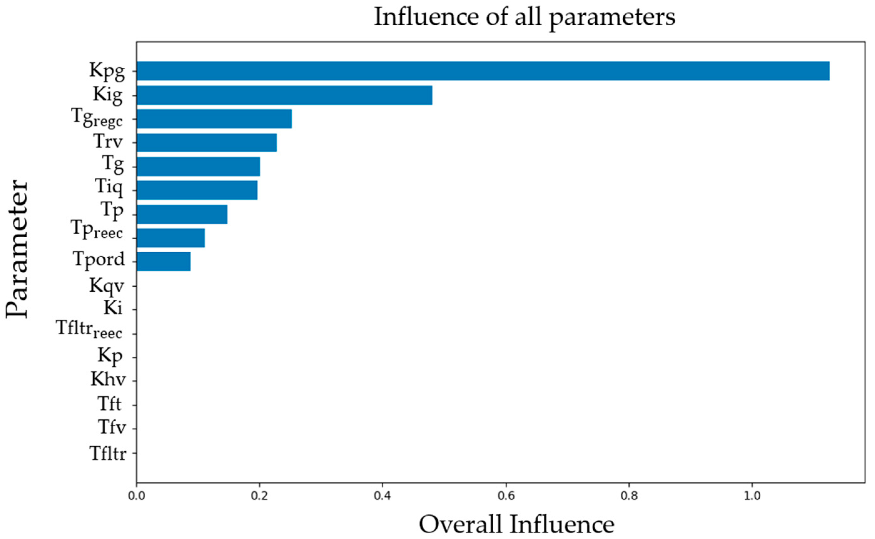
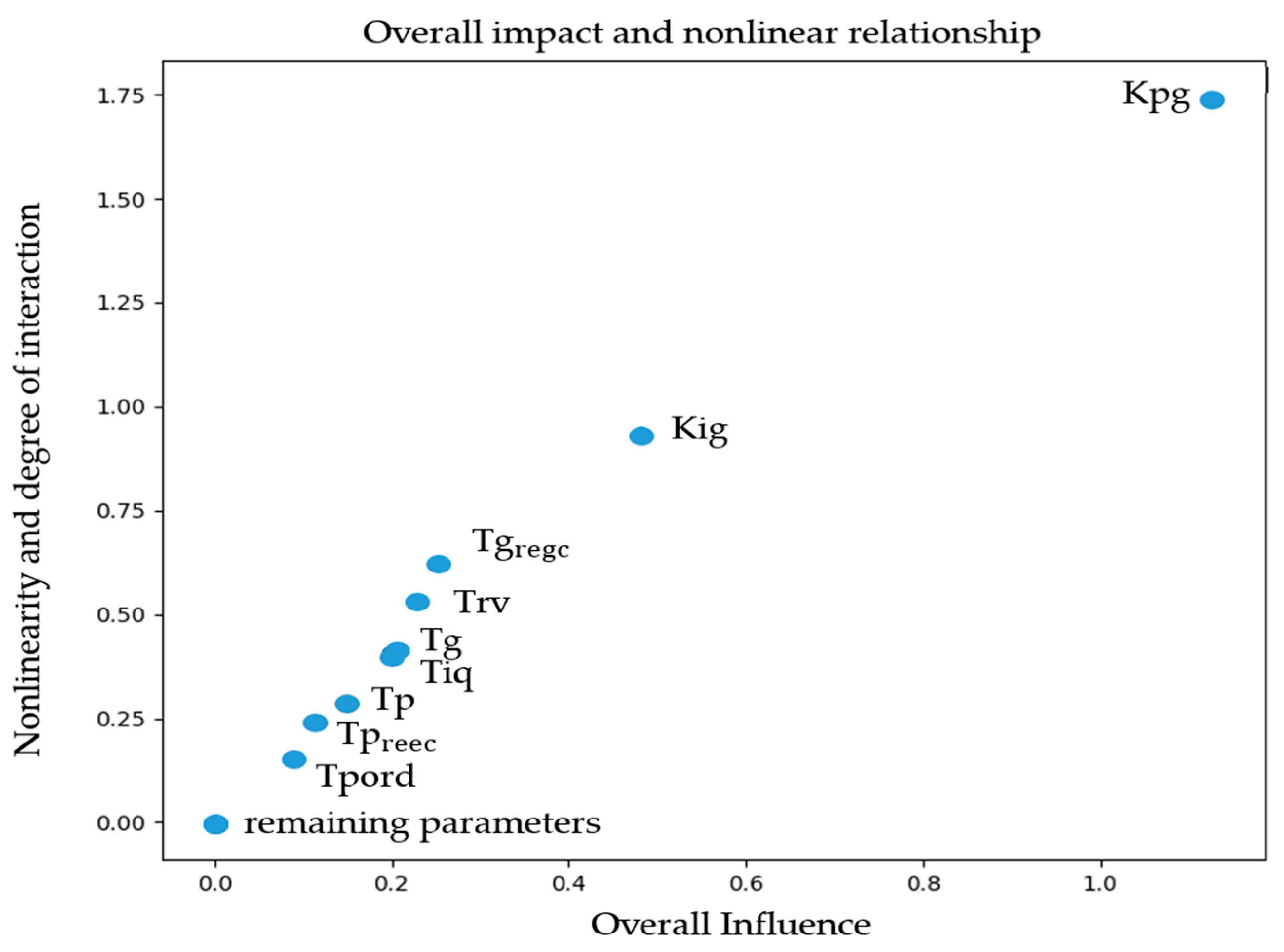
The Morris analysis uses the WECC energy storage model’s default settings as the baseline and evaluates performance using five frequency metrics. The parameter space is sampled with L = 20 OAT trajectories and 10 discrete levels. One parameter is perturbed at a time along each trajectory, and simulations are run to obtain frequency responses and compute the score and elementary effects. Aggregated effects are then used to estimate the mean influence, overall magnitude, and variability for parameter ranking. Figure 11 shows the ranking of influential parameters, and Figure 12 (scatter plot) helps identify potential nonlinearity or interaction effects.

Figure 11 shows that Kpg has the largest overall influence on frequency, followed by Kig. Time constants (e.g., ${\mathrm{T}\mathrm{g}}_{regc}$, Trv, Tg, Tiq, and Tp) have moderate effects, while the remaining parameters are much less influential. Combining Figure 11 and Figure 12 further suggests that Kpg and Kig exhibit stronger nonlinearity and interaction effects, whereas moderate- and low-impact parameters mainly lie in low-to-medium and low-nonlinearity regions, respectively, implying more straightforward and stable impacts on frequency dynamics.

Figure 11 and Figure 12 indicate that Kpg and Kig fall in the high-impact, high-nonlinearity region, identifying them as core gains that directly govern power output under frequency deviations. Changes in these gains affect both regulation strength and control behavior, explaining their top influence in Figure 11. By contrast, time constants (e.g., Tg, Trv, Tiq, and Tp) show moderate impact and low nonlinearity, implying that they mainly shape response speed and transient recovery rather than regulation intensity. Filter and auxiliary-control parameters cluster in the low-impact, low-nonlinearity region, suggesting limited contribution beyond signal smoothing and supportive stabilization.

In summary, Morris sensitivity results provide a practical basis for BESS controller tuning by prioritizing the most influential parameters, thereby improving frequency regulation and system reliability.

Table 3. Key Parameters Identified by Morris Sensitivity Analysis.

Model	Parameter	Morris Rank
REPC_A	Kpg	1
	Kig	2
	Tp	7
	Tg	5
REEC_C	Tp	8
	Trv	4
	Tiq	6
	Tpord	9
REGC_A	Tg	3

lists the key parameters identified in this study and is used as the reference set for subsequent algorithm analysis and controller optimization.

4.4. Algorithm Results and Analysis

Before optimization, algorithm hyperparameters must be defined. For a fair comparison, the iteration number and population size are fixed across algorithms (

Table 4. Shared Parameters Across Algorithms.

Parameter	Denotation	Value
SWARMSIZE	Population size	10
MAXITER	Maximum number of iterations	50

). Algorithm-specific settings are then specified—IGA uses crossover, mutation, and elitism (Section 3.2), while GWO uses control coefficients (Section 3.4). IGA/GWO settings are summarized in

Table 5. Optimization Mechanism Parameters for Each Algorithm.

Algorithm	Parameter	Denotation	Value
IGA	Pc	Mating rate	0.9
	Pm	Mutation rate	0.15
	Elite	Elite Retention	0.1
	Omega	Mating weight	0.5
GWO	a	Dynamic adjustment parameters	2
	r1	random variable1	[0, 1]
	r2	random variable2	[0, 1]

, and controller parameter search ranges, which are selected based on Ref. [36], are given in

Table 6. Battery Energy Storage Controller Parameter Ranges.

Model	Parameter	Value
REPC_A	Kpg	0.0001~50
	Kig	0.0001~50
	Tp	0.02~0.5
	Tg	0.05~0.5
REEC_A	Tp	0.0001~0.1
	Trv	0.0001~0.1
	Tiq	0.0001~0.1
	Tpord	0.01~0.1
REGC_A	Tg	0.01~0.05

.

4.4.1. Scenario 1: One Wind Turbine Reduced to Half Load

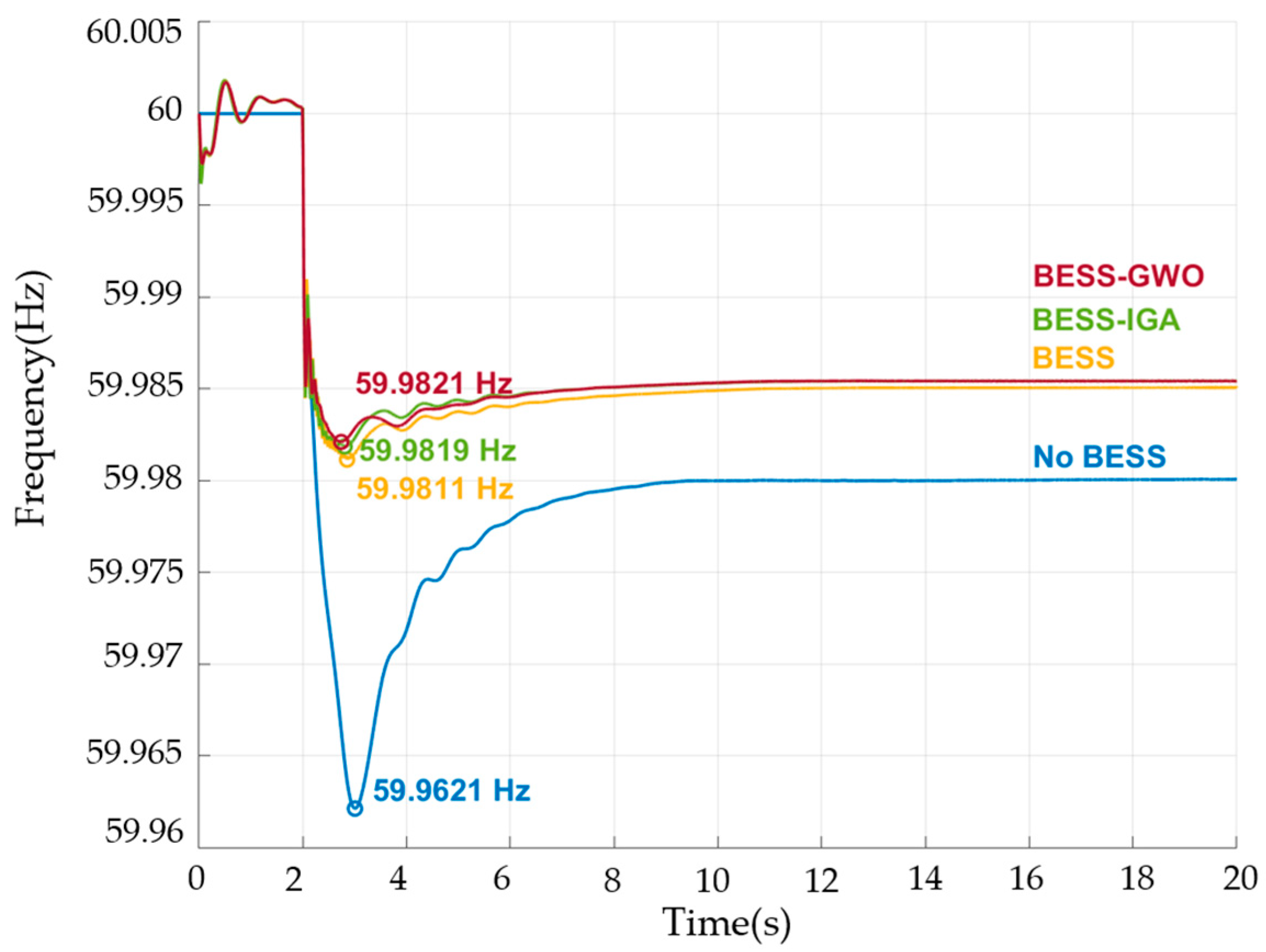
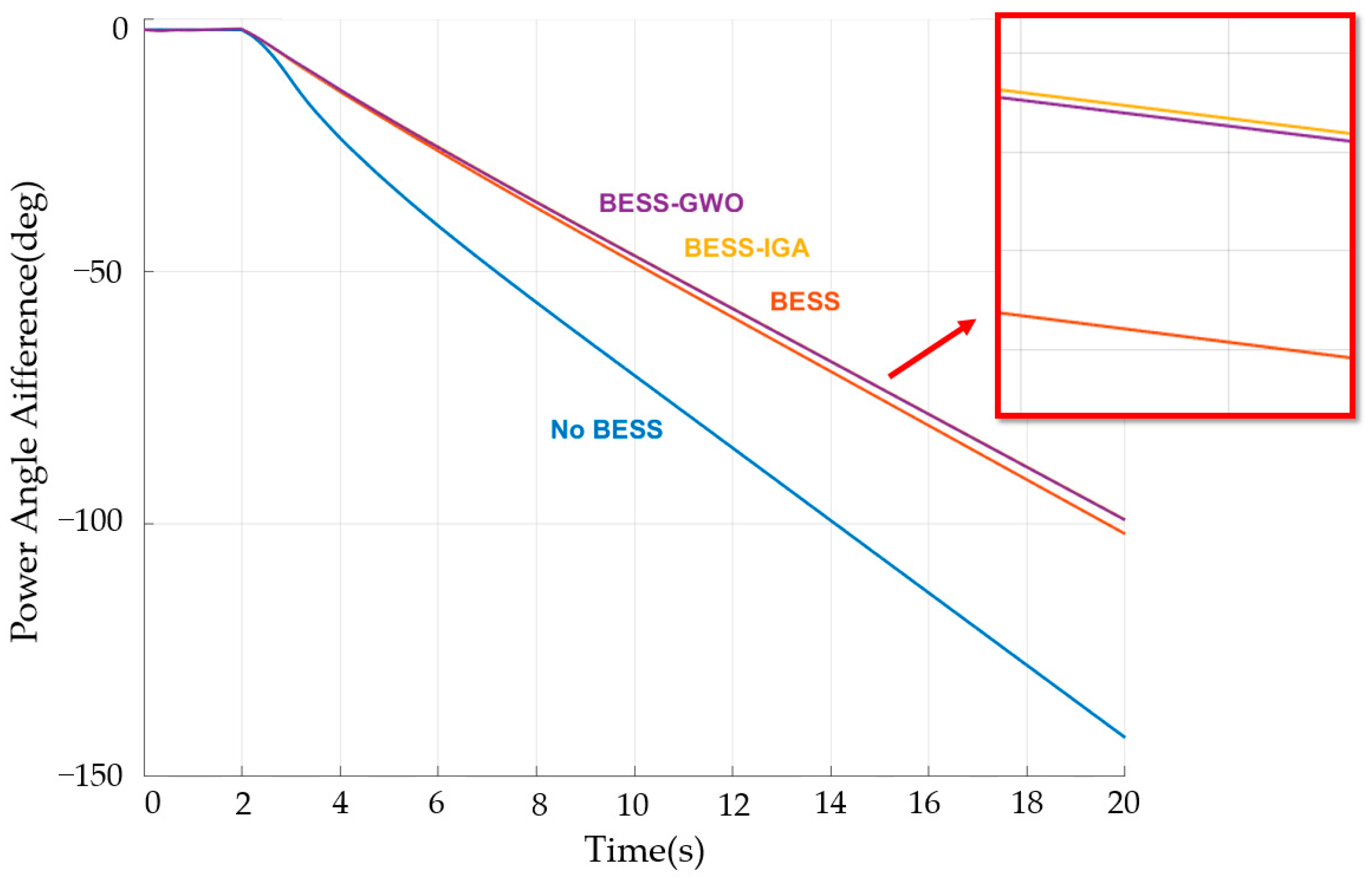
At 2 s, one wind turbine is reduced to half load to evaluate system dynamics under different ESS configurations. Four cases are compared: no ESS, ESS without optimization, ESS optimized by IGA, and ESS optimized by GWO. Figure 13 shows the frequency responses, and Figure 14 shows the corresponding equivalent power-angle difference in the ESS unit relative to the center of inertia variations.

Figure 13 shows that after the disturbance at 2 s, the no-ESS case experiences the largest frequency drop, with a nadir of about 59.9621 Hz, indicating weak frequency support. With ESS, the nadir improves to 59.9811 Hz, and further optimization raises it to 59.9819 Hz (IGA) and 59.9821 Hz (GWO) with a smoother recovery. Overall, ESS markedly enhances frequency dynamics, and optimized control further improves frequency support and post-disturbance stability.

Figure 14 indicates that without ESS, the equivalent power-angle difference in the ESS unit relative to the center of inertia (COI) reaches 142.425°, implying the weakest synchronizing stability. With ESS, it decreases to 102.019°, showing effective suppression of angle deviations. With optimized control, it further drops to 99.273° (GWO) and 99.189° (IGA), both better than the non-optimized case, with IGA slightly superior. Overall, ESS improves equivalent power-angle stability, and parameter optimization further strengthens post-disturbance synchronism.

4.4.2. Scenario 2: Single Wind Turbine Shutdown

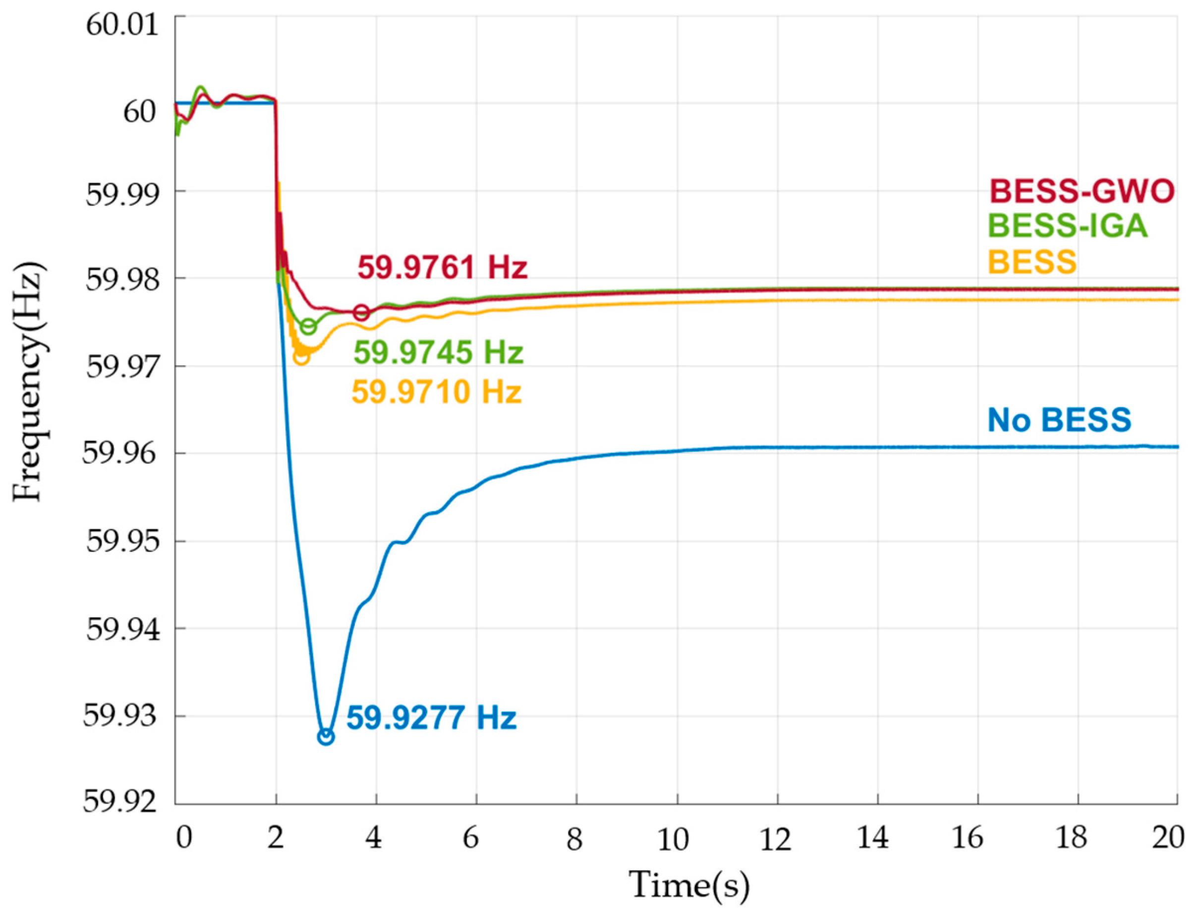
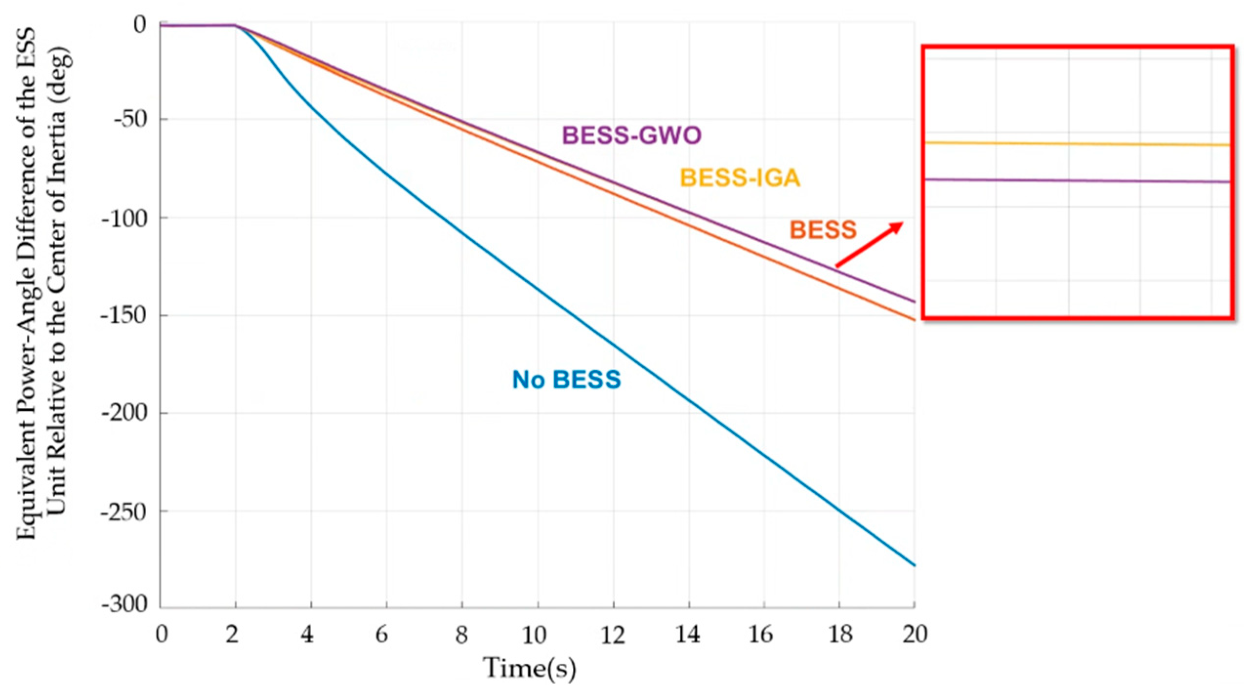
Figure 15 shows the frequency responses for different configurations in Scenario 2, and Figure 16 shows the corresponding time-varying equivalent power-angle difference in the ESS unit relative to the center of inertia.

Figure 15 shows that without ESS, the frequency drop is most severe, with a nadir of 59.9277 Hz and a slower recovery. With ESS, the nadir improves to 59.9710 Hz. Optimization further raises it to 59.9745 Hz (IGA) and 59.9761 Hz (GWO) with a smoother recovery, with GWO performing best. Overall, ESS improves frequency dynamics, and optimization further strengthens post-disturbance frequency stability in Scenario 2.

Figure 16 shows clear differences in end-of-simulation equivalent power-angle differences in the ESS unit relative to the center of inertia across configurations. Without ESS, it reaches 278.067° (weakest synchronism), while adding ESS improves it to 152.603°, indicating effective suppression of angle deviations. With optimized control, it further improves to 143.395° (GWO) and 143.291° (IGA), both better than the non-optimized ESS case, with IGA slightly superior. Overall, ESS enhances equivalent power-angle stability, and optimization further strengthens post-disturbance synchronism in Scenario 2.

4.4.3. Scenario 3: Three Wind Turbines Reduced to Half Load

Figure 17 shows the frequency responses for different configurations in Scenario 3, and Figure 18 shows the corresponding time-varying equivalent power-angle difference in the ESS unit relative to the center of inertia.

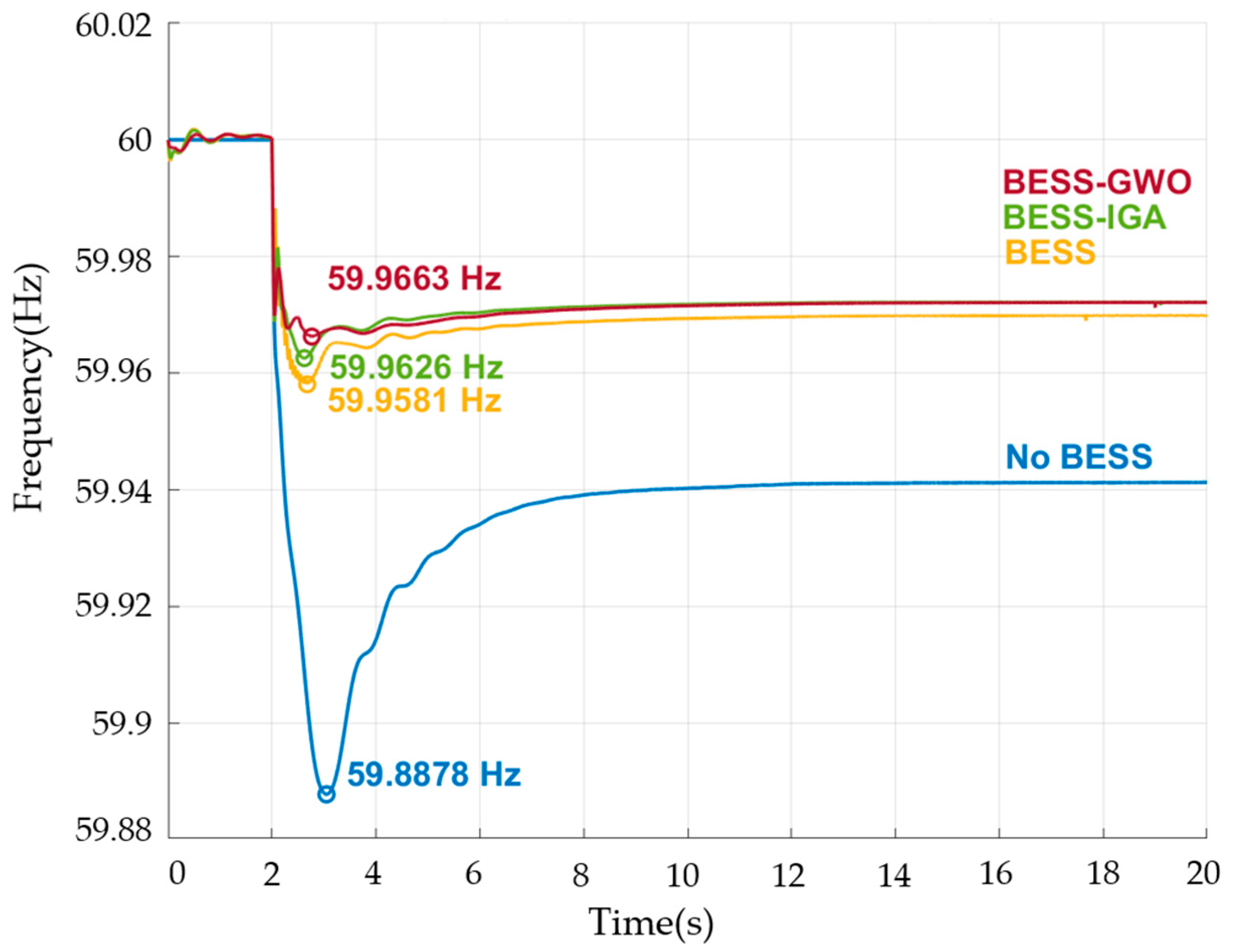
Figure 17 shows that without ESS, the frequency drop is largest, with a nadir of 59.8878 Hz and slower recovery. With ESS, the nadir improves to 59.9581 Hz. Optimization further raises it to 59.9626 Hz (IGA) and 59.9663 Hz (GWO) with a more stable recovery, with GWO performing best. Overall, Scenario 3 confirms that optimization-based tuning strengthens ESS frequency regulation and improves frequency stability.

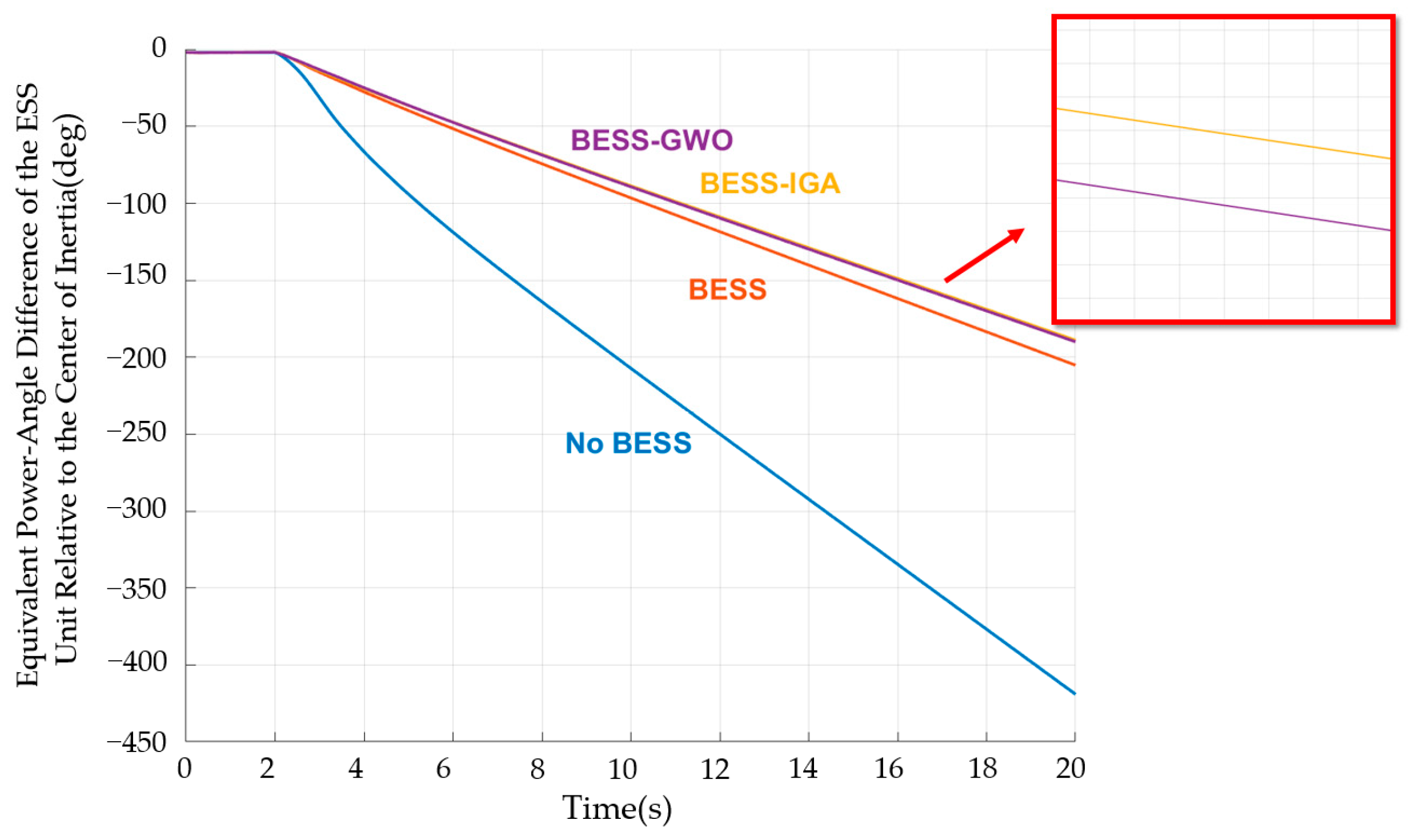
Figure 18 shows that without ESS, the equivalent power-angle difference in the ESS unit relative to the center of inertia reaches 419.143° (weakest synchronism), while adding ESS reduces it to 205.244°, indicating effective suppression of angle divergence. With optimized control, it further improves to 190.035° (GWO) and 188.953° (IGA), with IGA performing better. Overall, ESS improves equivalent power-angle stability, and optimization-based tuning further enhances synchronizing capability.

4.4.4. Scenario 4: An N-1 Contingency Corresponding to the Tripping of the Largest Synchronous Generator in the System

Figure 19 shows the frequency responses for different configurations in Scenario 4, and Figure 20 presents the corresponding time-varying equivalent power-angle difference in the ESS unit relative to the center of inertia (COI).

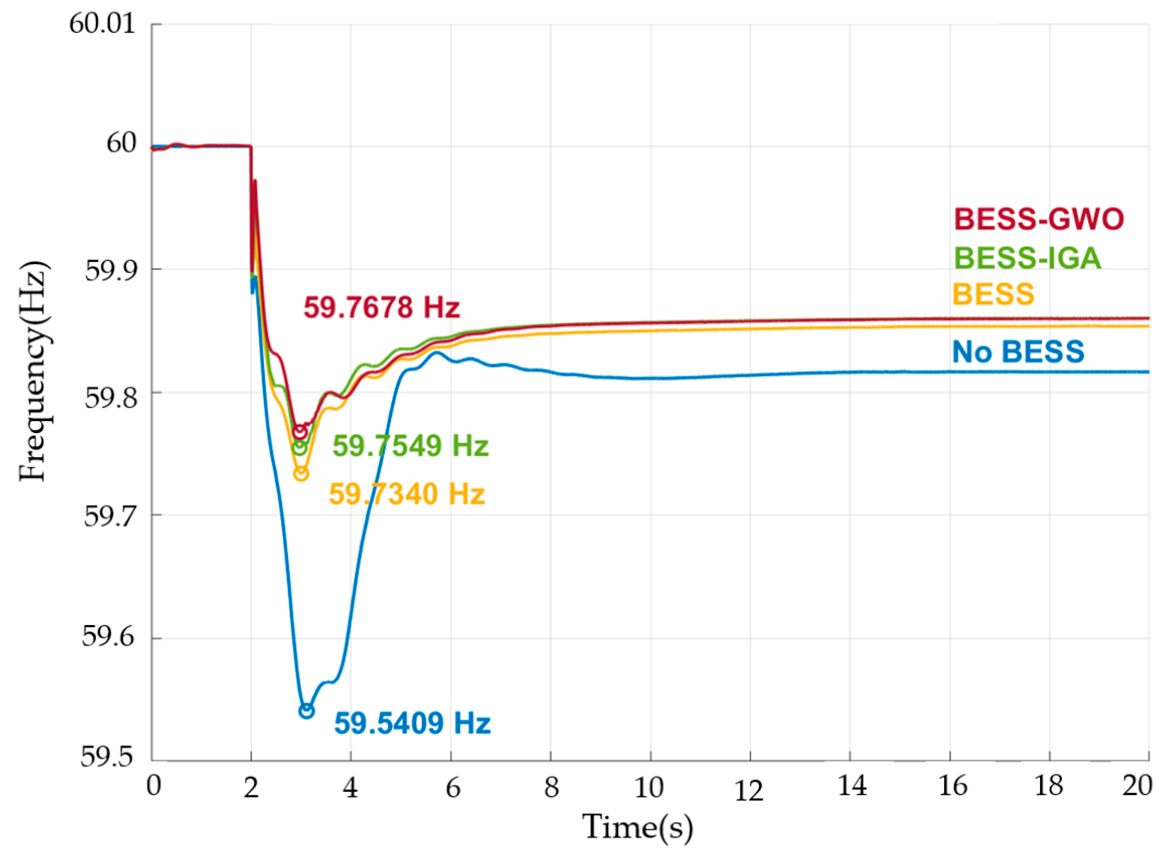
Figure 19 shows the without energy storage, the system exhibits the most severe frequency drop, with a minimum frequency of 59.5409 Hz. The inclusion of a non-optimized BESS improves the frequency nadir to 59.7340 Hz, while optimized BESS control further enhances performance, increasing the minimum frequency to 59.7549 Hz with IGA and to 59.7678 Hz with GWO. These results confirm that the proposed optimization framework effectively mitigates frequency deviations under the worst-case contingency, with GWO providing superior frequency-support performance compared with IGA.

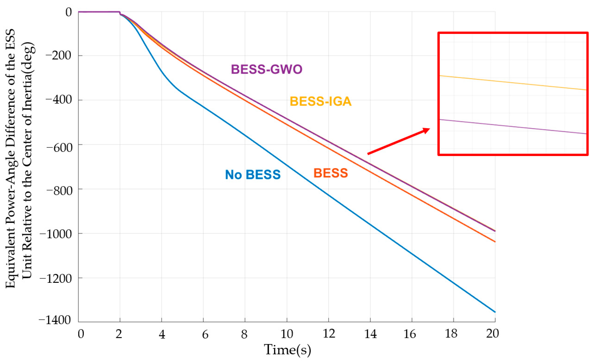
Figure 20 shows the equivalent power-angle difference in the ESS unit relative to the center of inertia under Scenario 4 (N-1 tripping of the largest synchronous generator). Without BESS, the angular deviation reaches 1356°, while a non-optimized BESS reduces it to 1036°. With optimized control, the equivalent power-angle difference is further reduced to 991° with GWO and to 989° with IGA, confirming that the proposed framework significantly improves angular stability under the worst-case contingency.

5. Conclusions

This study develops a PSS^®E dynamic model of the IEEE New England 39-bus system with three wind turbines and two BESS units. Four disturbance scenarios are considered to represent moderate-to-severe operating conditions: (i) single-turbine half-load, (ii) single-turbine trip, (iii) three-turbine half-load, and (iv) an N-1 contingency corresponding to the tripping of the largest synchronous generator in the system. Key control parameters are first screened using Morris sensitivity analysis to reduce the search dimension, and controller tuning is then performed using IGA and GWO with frequency metrics as the optimization objective. Performance is evaluated using frequency dynamics and the equivalent power-angle difference in the ESS unit relative to the center of inertia.

Across all scenarios (Figure 13, Figure 14, Figure 15, Figure 16, Figure 17, Figure 18, Figure 19 and Figure 20), adding BESS improves both frequency and equivalent power-angle dynamics of the ESS unit relative to the center of inertia by reducing the frequency drop and accelerating recovery, indicating effective fast frequency support. Compared with the non-optimized case, both IGA and GWO further improve the frequency nadir and smooth recovery; GWO is slightly better in nadir suppression. For the equivalent power-angle difference in the ESS unit relative to the center of inertia, optimization further reduces the maximum separation, with IGA showing a small advantage. Overall, algorithm-based tuning enhances BESS frequency regulation and system dynamic stability.

This work has two main limitations: (i) disturbances are modeled as single events rather than continuous, stochastic, or compounded disturbances, and (ii) the BESS configuration is fixed, without exploring capacity sizing, installation location, or multi-BESS coordinated control. Future work will incorporate stochastic or measured wind data to assess long-term robustness, and extend the framework to include BESS sizing/placement and coordinated control to validate applicability under different system structures and high wind penetration.

References

1. Ulbig, A.; Borsche, T.; Andersson, G. Impact of Low Rotational Inertia on Power System Stability and Operation. IFAC Proc. Vol. 2014, 47, 7290–7297. [Google Scholar] [CrossRef] [Scilit]
2. Milano, F.; Dörfler, F.; Hug, G.; Hill, D.J.; Verbič, G. Foundations and Challenges of Low-Inertia Systems (Invited Paper). In Proceedings of the 2018 Power Systems Computation Conference (PSCC), Dublin, Ireland, 11–15 June 2018; IEEE: New York, NY, USA, 2018; pp. 1–25. [Google Scholar]
3. Meng, L.; Zafar, J.; Khadem, S.K.; Collinson, A.; Murchie, K.C.; Coffele, F. Fast Frequency Response from Energy Storage Systems—A Review of Grid Standards, Projects and Technical Issues. IEEE Trans. Smart Grid 2020, 11, 1566–1581. [Google Scholar] [CrossRef] [Scilit]
4. Lu, C.-F.; Liu, C.-C.; Wu, C.-J. Effect of battery energy storage system on load frequency control considering governor deadband and generation rate constraint. IEEE Trans. Energy Convers. 1995, 10, 555–561. [Google Scholar] [CrossRef] [Scilit]
5. Padhy, S.; Panda, S. Application of a simplified Grey Wolf optimization technique for adaptive fuzzy PID controller design for frequency regulation of a distributed power generation system. Prot. Control Mod. Power Syst. 2021, 6, 2. [Google Scholar] [CrossRef] [Scilit]
6. Moradi-Shahrbabak, Z. A genetic approach to design an SSR damping controller in a hybrid photovoltaic-battery system by considering the state of charge. J. Energy Storage 2025, 108, 115003. [Google Scholar] [CrossRef] [Scilit]
7. Ghatuari, I.; Kumar, N.S. Controller design and optimal sizing of battery energy storage system for frequency regulation in a multi machine power system. Energy Rep. 2024, 12, 4757–4776. [Google Scholar] [CrossRef] [Scilit]
8. Wang, S.; Yue, Y.; Cai, S.; Li, X.; Chen, C.; Zhao, H.; Li, T. A Comprehensive Survey of the Application of Swarm Intelligent Optimization Algorithm in Photovoltaic Energy Storage Systems. Sci. Rep. 2024, 14, 68964. [Google Scholar] [CrossRef] [Scilit]
9. Lin, C. An Adaptive Genetic Algorithm Based on Population Diversity Strategy. In Proceedings of the 2009 Third International Conference on Genetic and Evolutionary Computing, Guilin, China, 14–16 October 2009; IEEE: New York, NY, USA, 2009; pp. 93–96. [Google Scholar]
10. Srinivas, M.; Patnaik, L.M. Adaptive probabilities of crossover and mutation in genetic algorithms. IEEE Trans. Syst. Man Cybern. 1994, 24, 656–667. [Google Scholar] [CrossRef] [Scilit]
11. Leung, Y.; Gao, Y.; Xu, Z.-B. Degree of population diversity—A perspective on premature convergence in genetic algorithms and its Markov chain analysis. IEEE Trans. Neural Netw. 1997, 8, 1165–1176. [Google Scholar] [CrossRef] [Scilit]
12. Mirjalili, S.; Mirjalili, S.M.; Lewis, A. Grey wolf optimizer. Adv. Eng. Softw. 2014, 69, 46–61. [Google Scholar] [CrossRef] [Scilit]
13. Mohanty, S.; Subudhi, B.; Ray, P.K. A New MPPT Design Using Grey Wolf Optimization Technique for Photovoltaic System Under Partial Shading Conditions. IEEE Trans. Sustain. Energy 2016, 7, 181–188. [Google Scholar] [CrossRef] [Scilit]
14. Campolongo, F.; Cariboni, J.; Saltelli, A. An effective screening design for sensitivity analysis of large models. Environ. Model. Softw. 2007, 22, 1509–1518. [Google Scholar] [CrossRef] [Scilit]
15. Hasan, K.N.; Preece, R.; Milanović, J.V. Priority Ranking of Critical Uncertainties Affecting Small-Disturbance Stability Using Sensitivity Analysis Techniques. IEEE Trans. Power Syst. 2017, 32, 2629–2639. [Google Scholar] [CrossRef] [Scilit]
16. Qin, C.; Jin, Y.; Tian, M.; Ju, P.; Zhou, S. Comparative Study of Global Sensitivity Analysis and Local Sensitivity Analysis in Power System Parameter Identification. Energies 2023, 16, 5915. [Google Scholar] [CrossRef] [Scilit]
17. Yu, Y.; Shan, K.; Wang, S. Global sensitivity analysis of key parameters for data center power and energy systems considering reliability. Energy Proc. 2025, 52, 1–7. [Google Scholar] [CrossRef] [Scilit]
18. Wei, H.; Wang, J.; Shan, Y.; Guo, Z.; Ma, J. Application of Sobol Sensitivity Analysis with Surrogate Model of Analytical Function. In Proceedings of the 2022 IEEE 2nd International Conference on Power, Electronics and Computer Applications (ICPECA), Shenyang, China, 21–23 January 2022; IEEE: New York, NY, USA, 2022; pp. 504–509. [Google Scholar]
19. Abera, B.; Wik, T.; Bekele, G.; Mamo, M. Parametric Sensitivity Analysis of the Modified AMOCO Model for an Anaerobic Digester. In Proceedings of the 2024 IEEE PES/IAS PowerAfrica, Johannesburg, South Africa, 7–11 October 2024; IEEE: New York, NY, USA, 2024; pp. 1–5. [Google Scholar]
20. Energy Systems Integration Group (ESIG). WT3—Generic Wind Model. Available online: https://esig.energy/wiki-main-page/wt3-generic-wind-model/ (accessed on 6 January 2026).
21. Cupelli, M.; Doig Cardet, C.; Monti, A. Voltage stability indices comparison on the IEEE-39 bus system using RTDS. In Proceedings of the 2012 IEEE International Conference on Power System Technology (POWERCON), Auckland, New Zealand, 30 October–2 November 2012; IEEE: New York, NY, USA, 2012; pp. 1–6. [Google Scholar]
22. de Lisboa, U. WT3 Generic Models for Transient Stability Studies of Wind Power Generation. Available online: https://fenix.tecnico.ulisboa.pt/downloadFile/563345090415996/Resumo_Out-2017_DSE.pdf (accessed on 6 January 2026).
23. Lee, C.-C.; Hsin, Y.-M.; Dai, S.-C.; Kuo, C.-C. Optimal Modeling for Dynamic Response of Energy Storage Systems. Appl. Sci. 2023, 13, 4943. [Google Scholar] [CrossRef] [Scilit]
24. Saltelli, A.; Ratto, M.; Tarantola, S.; Campolongo, F. Sensitivity analysis: A review of recent advances. Eur. J. Oper. Res. 2016, 248, 869–887. [Google Scholar] [CrossRef] [Scilit]
25. Morris, M.D. Factorial sampling plans for preliminary computational experiments. Technometrics 1991, 33, 161–174. [Google Scholar] [CrossRef]
26. Qi, B.; Hasan, K.N.; Milanović, J.V. Identification of Critical Parameters Affecting Voltage and Angular Stability Considering Load-Renewable Generation Correlations. IEEE Trans. Power Syst. 2019, 34, 2859–2869. [Google Scholar] [CrossRef] [Scilit]
27. Shi, W.; Chen, X. Controlled Morris method: A new factor screening approach empowered by a distribution-free sequential multiple testing procedure. Reliab. Eng. Syst. Saf. 2019, 189, 299–314. [Google Scholar] [CrossRef] [Scilit]
28. Mardle, S.; Pascoe, S. An overview of genetic algorithms for the solution of optimisation problems. Comput. High. Educ. Econ. Rev. 1999, 13, 16–20. [Google Scholar]
29. Whitley, D. A genetic algorithm tutorial. Stat. Comput. 1994, 4, 65–85. [Google Scholar] [CrossRef] [Scilit]
30. datathrillz. How Genetic Algorithms Work. 10 August 2020. Available online: https://datathrillz.com/genetic-algorithm/?utm_source=chatgpt.com (accessed on 6 January 2026).
31. Lenin, K.; Reddy, B.R.; Kalavathi, M.S. A new improved GA and PSO combined hybrid algorithm (HIGAPSO) for solving optimal reactive power dispatch problem. J. Ind. Intell. Inf. 2014, 2, 205–209. [Google Scholar] [CrossRef] [Scilit]
32. Mirjalili, S.; Dong, J.S.; Lewis, A. (Eds.) Nature-Inspired Optimizers: Theories, Literature Reviews and Applications; Studies in Computational Intelligence; Springer: Cham, Switzerland, 2020; Volume 811. [Google Scholar]
33. Faris, H.; Aljarah, I.; Al-Betar, M.A.; Mirjalili, S. Grey wolf optimizer: A review of recent variants and applications. Neural Comput. Appl. 2018, 30, 413–435. [Google Scholar] [CrossRef] [Scilit]
34. Xing, Y.; Wang, D.; Wang, L. A Novel Dynamic Generalized Opposition-Based Grey Wolf Optimization Algorithm. Algorithms 2018, 11, 47. [Google Scholar] [CrossRef] [Scilit]
35. Xu, Z.; Yang, H.; Li, J.; Zhang, X.; Lu, B.; Gao, S. Comparative Study on Single and Multiple Chaotic Maps Incorporated Grey Wolf Optimization Algorithms. IEEE Access 2021, 9, 77416–77437. [Google Scholar] [CrossRef] [Scilit]
36. Wang, M.-H.; Chen, Y.-C.; Hung, C.-C. Research on Adaptive Control Optimization of Battery Energy Storage System Under High Wind Energy Penetration. Energies 2025, 18, 5057. [Google Scholar] [CrossRef] [Scilit]
37. Siemens Industry, Inc.; Siemens Power Technologies International. PSS®E 33.4 Model Library/Program Operation Manual; Siemens Industry, Inc.: Schenectady, NY, USA, 2013. [Google Scholar]
Figure 1. Wind & BESS Layout in IEEE 39-Bus.
Energies 19 00827 g001
Figure 2. Structural diagram of a wind turbine model.
Energies 19 00827 g002
Figure 3. WECC Generic BESS Control Architecture.
Energies 19 00827 g003
Figure 4. Schematic of Randomized OAT Trajectories.
Energies 19 00827 g004
Figure 5. Overall Procedure of Morris Sensitivity Analysis.
Energies 19 00827 g005
Figure 6. Crossover Operation Illustration.
Energies 19 00827 g006
Figure 7. IGA Flowchart.
Energies 19 00827 g007
Figure 8. Illustration of Grey Wolf Pack Hunting Stages.
Energies 19 00827 g008
Figure 9. GWO Flowchart.
Energies 19 00827 g009
Figure 10. Overall Experiment Flow Diagram.
Energies 19 00827 g010
Figure 11. Parameter Importance Ranking Plot.
Energies 19 00827 g011
Figure 12. Nonlinearity/Interaction Detection Plot.
Energies 19 00827 g012
Figure 13. System Frequency Responses Under Different Configurations in Scenario 1.
Energies 19 00827 g013
Figure 14. Equivalent Power-Angle Difference in the ESS Unit Relative to the Center of Inertia Under Different Configurations in Scenario 1.
Energies 19 00827 g014
Figure 15. System Frequency Responses Under Different Configurations in Scenario 2.
Energies 19 00827 g015
Figure 16. Equivalent Power-Angle Difference in the ESS Unit Relative to the Center of Inertia Under Different Configurations in Scenario 2.
Energies 19 00827 g016
Figure 17. System Frequency Responses Under Different Configurations in Scenario 3.
Energies 19 00827 g017
Figure 18. Equivalent Power-Angle Difference in the ESS Unit Relative to the Center of Inertia Under Different Configurations in Scenario 3.
Energies 19 00827 g018
Figure 19. System Frequency Responses Under Different Configurations in Scenario 4.
Energies 19 00827 g019
Figure 20. Equivalent Power-Angle Difference in the ESS Unit Relative to the Center of Inertia Under Different Configurations in Scenario 4.
Energies 19 00827 g020