Article

Data-Driven Site Selection Based on CO2 Injectivity in the San Juan Basin

Petroleum Recovery Research Center, New Mexico Institute of Mining and Technology, Socorro, NM 87801, USA
*
Author to whom correspondence should be addressed.
Energies 2026, 19(3), 764; https://doi.org/10.3390/en19030764 (registering DOI)
Submission received: 2 December 2025 / Revised: 10 January 2026 / Accepted: 15 January 2026 / Published: 1 February 2026
(This article belongs to the Collection Feature Papers in Carbon Capture, Utilization, and Storage)

Abstract

CO2 injection success hinges on the injectivity index, a major determinant of storage feasibility. This study develops a machine learning (ML)-driven framework optimized for CO2 injectivity prediction, benchmarking its robustness and real-world applicability against an empirical correlation developed in the literature. The framework is applied to the Entrada Formation in the San Juan Basin, a laterally extensive sandstone unit with limited structural complexity across most of the basin, except for localized uplift in the Hogback region. A numerical model was calibrated to perform sensitivity analysis to identify the dominant parameters influencing injectivity. A dataset of these parameters generated through experimental design informs the development of several ML-based proxies and the best model is selected based on error metrics. These metrics include coefficient of determination (R2), mean absolute error (MAE), and mean squared error (MSE). The effective permeability-thickness product was obtained by the Peaceman’s well model, fractional flow slope, and Dykstra–Parsons coefficient were identified as the most influential parameters impacting the objective function. Train–test and blind test validation identified the Ridge model as the best, achieving an R2 ≈ 0.994. The Ridge model which was used to map the Entrada Formation closely matches field-based correlations in the literature, confirming both its physical validity and the Entrada Formation’s strong injectivity potential, with slight deviations explained by the inclusion of additional parameters. This study reduces dependence on computationally intensive simulations while improving prediction accuracy. By benchmarking against established correlations, it enhances model reliability across diverse reservoir conditions. The proposed framework enables rapid, data-driven well placement and feasibility evaluations, streamlining decision-making for CO2 storage projects.

1. Introduction

Among carbon sequestration pathways, geological storage in deep saline aquifers offers the greatest long-term capacity [1]. However, the successful deployment of large-scale storage depends on overcoming significant technical and operational challenges, particularly those associated with CO2 injectivity, the ability of a formation to accept and transmit injected fluids under safe pressure conditions [2]. The heterogeneity of these formations, usually manifested as complex variations in porosity and permeability, further complicates injectivity assessment [3]. Such variability governs the pressure distribution and CO2 plume migration, often leading to unanticipated channeling [4]. Underestimating injectivity can result in over-conservative designs and inflated costs, while overestimating it risks wellbore overpressure or poor storage performance.
In addition to geological complexity, interactions between CO2, brine, and rock can dynamically modify injectivity through time [5]. Dissolution, precipitation, and fines migration near the wellbore can either enhance or impair permeability, depending on the local geochemical and geomechanical conditions [6]. For early-stage site screening, high-fidelity models are often impractical [7]. Indeed, a single simulation may require weeks of processing on high-performance computing systems, even when based on uncertain input data [8]. This mismatch between modeling precision and data availability has emerged as a central bottleneck in scaling carbon capture and storage (CCS): the tools capable of detailed analysis are too slow and data-hungry to inform the early decision-making processes that drive project development and policy action. Emerging research points to data-driven approaches, of which machine learning (ML) serves as a promising means to bridge this gap [9]. ML algorithms can extract governing patterns directly from limited datasets, offering rapid, data-driven estimates of injectivity that complement, rather than replace, physics-based simulations [10]. Yet, widespread skepticism persists due to the “black-box” nature of many ML models, which often achieve accuracy at the expense of physical interpretability [11]. For CCS applications, where safety, regulatory compliance, and geological plausibility are paramount, models must not only predict accurately but also explain why those predictions make sense in physical terms [12].
Previous research on CO2 injectivity assessment have employed numerical simulation, analytical and semi-analytical modeling, as well as data-driven approaches; however, in most cases, injectivity is not evaluated directly but inferred from secondary indicators such as pressure buildup, plume extent, or flow capacity. Numerical modeling approaches have historically been the standard choice for detailed assessments of CO2 injectivity, primarily because of their ability to simulate complex multiphase flow dynamics in geological formations. Researchers like Jun et al. [13] optimized CO2 injection scenarios in the Pohang Basin, demonstrating that strategic configurations such as the Two Vertical Wells with Brine Extraction (TVEI) technique could significantly enhance the storage capacity, resulting in an additional 712,600 tons of CO2 stored through active pressure management strategies. Nevertheless, Jun et al. [13] noted that extensive reservoir characterization data and substantial computational resources are required for good numerical optimization and uncertainty quantification.
Nordbotten et al. [14] developed an analytical model based on radial flow assumptions to predict the radial extent of CO2 plumes. Their model, expressed as t = C m a x t , was validated against numerical simulations, showing good accuracy for homogeneous reservoirs. However, Nordbotten et al. [14] acknowledge that such analytical models inherently assume idealized conditions like reservoir homogeneity and sharp fluid interfaces that significantly limit their applicability in heterogeneous and realistic geological contexts. Building upon these limitations, semi-analytical models have been proposed to partially bridge the gap between the simplicity of analytical methods and the realism of numerical simulations. Whittle et al. [15], for instance, introduced a two-zone radial composite model that accounts for temporal variations in near-well reservoir properties, offering enhanced realism compared to purely analytical solutions. Nonetheless, their model remains constrained by assumptions that limit its capability to represent complex reservoir dynamics fully.
Data-driven approaches, including statistical surrogate modeling, have gained attention in recent years for their potential to estimate injectivity parameters. Mishra et al. [16] successfully employed Latin hypercube sampling (LHS)-based statistical models to replicate numerically the derived cumulative distribution functions for critical injectivity-related parameters such as plume radius and pressure buildup, demonstrating substantial computational savings without substantial losses in accuracy. Similarly, Valluri et al. [17] developed a straightforward empirical correlation linking the injectivity index directly with reservoir permeability thickness ( J = 0.08 × k h ). This simplified model provides rapid injectivity assessments useful in preliminary reservoir evaluations, although it remains limited by the representativeness of the training data and in their ability to incorporate multiple interacting controls on injectivity. While these approaches enable rapid injectivity estimation, they often rely on simplified or indirect relationships and are limited in their ability to represent the combined influence of geological heterogeneity and operational controls. These limitations motivate the development of a hybrid framework that integrates physics-based simulation with data-driven modeling for more robust injectivity prediction.
Accurate assessment of CO2 injectivity also depends on how reservoir simulations represent near-wellbore flow and well–reservoir coupling [18]. In numerical models, injectivity is not computed directly but inferred from the simulated injection rate and pressure response [19]. In the ECLIPSE simulator, this relationship is governed by the Peaceman well formulation, which defines an equivalent well radius used to compute the effective permeability-thickness product ( k h ) reported by the simulator [20]. The Peaceman radius accounts for grid geometry, permeability anisotropy, and therefore implicitly influences simulated bottomhole pressure and derived injectivity metrics. Previous studies have shown that gas injection performance is sensitive to well representation, non-Darcy flow effects, and pressure-dependent properties, particularly in heterogeneous reservoirs [21]. Integrated reservoir–well modeling for gas storage further demonstrates that the predicted injection capacity depends on the numerical representation of wells [22]. These considerations motivate the use of physics-based simulations to establish consistent injectivity behavior while supporting the development of efficient surrogate models for early-stage screening.
This study presents a hybrid modeling framework for predicting CO2 injectivity in heterogeneous saline formations, using the Entrada Sandstone of the San Juan Basin as a representative case. The goal is to develop a machine learning proxy that can be used during early-stage site evaluation while remaining consistent with the key physical controls on injectivity. The work is structured in a stepwise manner. First, a calibrated numerical reservoir model is used to examine the sensitivity of CO2 injectivity to geological and operational parameters and to identify the dominant controlling factors. Next, a suite of machine learning models is trained and evaluated to determine a proxy capable of accurately reproducing injectivity behavior. The selected model is then assessed through comparison with an established field data-based injectivity correlation to evaluate its robustness beyond the training data. Finally, the validated framework is applied to generate an injectivity map of the Entrada Formation to illustrate the spatial variability in injection potential.

2. Materials and Methods

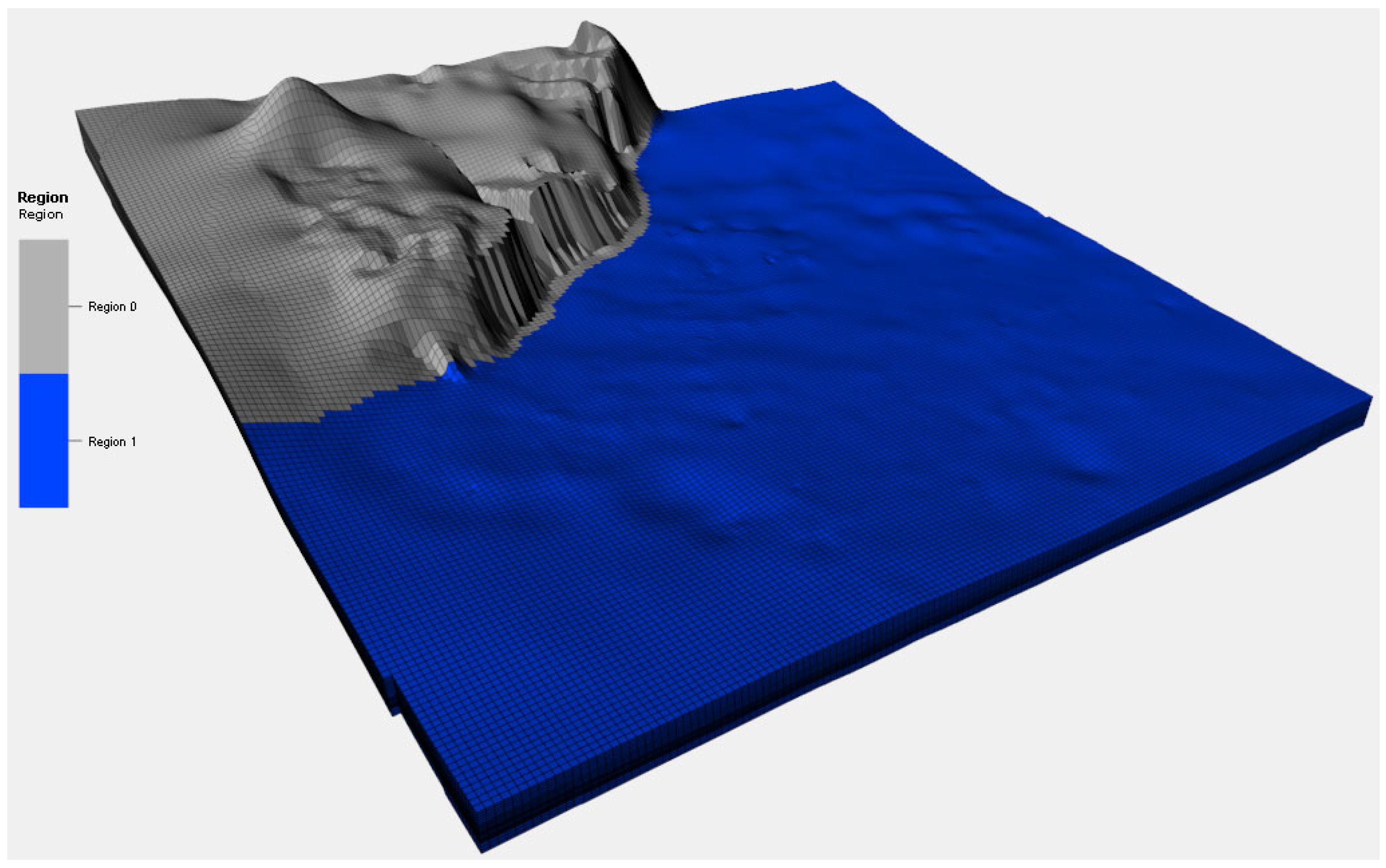
The methodology followed a structured workflow designed to integrate geological interpretation, dynamic modeling, and data-driven prediction to assess CO2 injectivity in the Entrada Sandstone. As illustrated in Figure 1, the process began with the integration of geological, geophysical, and petrophysical datasets to construct a three-dimensional (3D) static geological model representing lithology, porosity, and permeability distributions, and the structural–stratigraphic framework. The porosity data were obtained from density porosity logs from 21 wells and calibrated against available core data, while permeability was derived from the calibrated porosity and distributed in three dimensions using stochastic geostatistical interpolation approach. Compositional fluid properties and saturation profiles were incorporated to represent in situ conditions. These datasets collectively formed the foundation for a 3D hydrodynamic model, which was developed to simulate fluid flow and pressure propagation, thereby enabling realistic predictions of CO2 injection performance and plume migration. The governing flow equations were solved using the finite difference formulation implemented in the ECLIPSE reservoir simulator [20]. All simulations were performed on a high-performance workstation with dual Intel Xeon Gold processors, 64 CPU cores, and 256 GB of RAM. The model, as seen in Figure 2, consists of a shallow hogback region where pressures are very low. These act as low-pressure outliers that depress the average field pressure, leading to an overestimation of injectivity in the main basin region where injection takes place; as a result, the grid cells at hogback region are made inactive to curb this bias. The hydrodynamic model was then built in compositional mode to accurately represent CO2–brine interactions and phase behavior during injection. CO2 was defined at molecular weight of 44.01 g/mol with brine density set to 62.46 lbm/ft3 (1000.51 kg/m3) and brine compressibility of 3.6 × 10⁻⁶ psi−1, indicating a moderately saline aquifer [23]. Furthermore, relative permeability was described using Corey exponents based on laboratory guidance [24]. The gas phase had an endpoint relative permeability of 0.55 and a Corey exponent of 3, while water relative permeability used a connate water saturation of 0.55 and the same exponent. Rock compressibility was modeled using the Newman [25] correlation for consolidated sandstone, with a minimum pressure of 2800 psi to capture pore volume changes during pressure buildup or decline. Together, the compositional and rock–fluid property inputs, as well as injection wells, defined a robust hydrodynamic framework for predicting injectivity and plume evolution.
Following model construction, the workflow transitioned into the calibration and predictive phases. Model calibration was achieved through history matching, where simulated results were adjusted to minimize discrepancies with observed water injection and pressure data. Sensitivity testing revealed that permeability exerted the strongest control on matching performance, prompting iterative refinement through permeability multipliers. A global permeability adjustment alone proved inadequate, so a localized approach was adopted, resulting in a close match between simulated and observed BHP trends, ensuring both statistical alignment and geological plausibility. The history-matched model then served as a baseline for CO2 injection forecasting, providing a reference case for injectivity under representative reservoir conditions. The calibrated model was used to simulate a 30-year CO2 injection scenario targeting the SJB Carbon Safe Strat Test #001 well. Injection was modeled as a 100% supercritical CO2 stream at a surface rate of 18 MMSCF/day and a bottomhole pressure limit of 4700 psi which is approximately 90% of the estimated fracture pressure, to maintain operational safety. Injectivity was computed in Eclipse using a User-Defined Quantity (UDQ) based on well gas injection rate (WGIR), bottomhole pressure (WBHP), and field average pressure (FPRP). The results provided the baseline injectivity profile and dynamic response used for subsequent sensitivity.
In order to quantify parameter sensitivities, a series of controlled simulations were performed to assess how key variables such as permeability-thickness product ( k h ), anisotropy, Dykstra–Parsons heterogeneity coefficient, injection flow rate, bottomhole pressure, and slope of fractional flow which affect injectivity response [2]. The parameter space was explored using Latin hypercube sampling (LHS) to ensure efficient coverage of all variable combinations [26]. Relative permeability was described using Corey correlations, where exponents for water and CO2 gas were varied between 1–3 and 3–5, respectively, guided by the literature [27,28]. The resulting relative permeability curves were used to compute fractional flow of CO2, f g , according to the following [29]
f g = k r g μ g k r g μ g + k r w μ w
where k r g and k r w represent gas and water relative permeabilities, and μ g and μ w are the gas and water viscosities respectively (averagely 0.05 cP for CO2 and 1.12 cP for brine at the base case simulation). The slope of the fractional flow curve (df/ds) was derived to characterize CO2–brine mobility contrast [30] through relative permeability relations.
Anisotropy varied from 0.1 to 0.6 [31], injection rate from 10 to 25 MMSCF/day, and BHP from 4000 to 4900 psi. These ranges provided a physically consistent envelope for evaluating injectivity under varying subsurface conditions. Spatial variability was addressed by analyzing varied well locations distributed across distinct hydraulic flow units of the Entrada Formation. For each well site, effective k h values were obtained and heterogeneity coefficients are determined using the Dykstra–Parsons (VDP) coefficient equation [32]:
V D P = k 50 k 84.1 k 50
where k 50 is the median permeability and k 84.1 is the permeability at the 84.1st percentile of the permeability distribution.
Data preprocessing involved several key steps. The most dominant variables exhibiting high skewness, particularly the effective k h and injectivity index values, were log-transformed to stabilize variance [33]. Nonlinear relationships were captured through polynomial feature expansion [34], and all variables were standardized to ensure uniform scaling across algorithms [35]. This polynomial expansion allows variable interactions and curvature effects to be captured through higher-order and cross-product terms, enabling linear models to approximate nonlinear responses. By embedding nonlinear structure into the feature space, polynomial expansion improves the linear models’ expressiveness while maintaining transparency and stable training behavior [34]. To ensure reliable model evaluation, a train–test split sensitivity study was conducted [36], systematically varying the test size between 10% and 40%. The optimal ratio was selected based on the R2 across all models to balance bias and variance. The Ridge, Least Absolute Shrinkage and Selection Operator (Lasso), ElasticNet, Response Surface, Random Forest, Extreme Gradient Boosting (XGBoost), and Light Gradient-Boosting Machine (LightGBM) models underwent hyperparameter optimization using GridSearchCV with five-fold cross-validation, targeting the highest achievable R2 values [37]. The model suite was selected to balance interpretability, predictive capability, and robustness in the presence of the heterogeneous controls on injectivity. Regularized linear models (Ridge, Lasso, and ElasticNet) were included to provide traceable relationships between injectivity and the controlling parameters, while mitigating multicollinearity commonly observed in geological datasets. The Response Surface model was employed as an intermediate-complexity proxy to represent smooth, nonlinear trends and parameter interactions without assuming a strictly linear response. More flexible ensemble and boosting models (Random Forest, XGBoost, and LightGBM) were incorporated to capture higher-order interactions and complex nonlinear behavior [38]. The inclusion of models spanning a range of complexity enables a systematic comparison between simpler regression-based proxies and high-capacity learners. The final model evaluation was based on R2, mean squared error (MSE), and residual analysis for training, testing, and blind datasets. The final optimized proxy model was implemented by mapping it across the Entrada Formation after further field validation which was performed by comparing the predictions made by the best model selected to the injectivity correlation envelope developed by Mishra et al. [39].
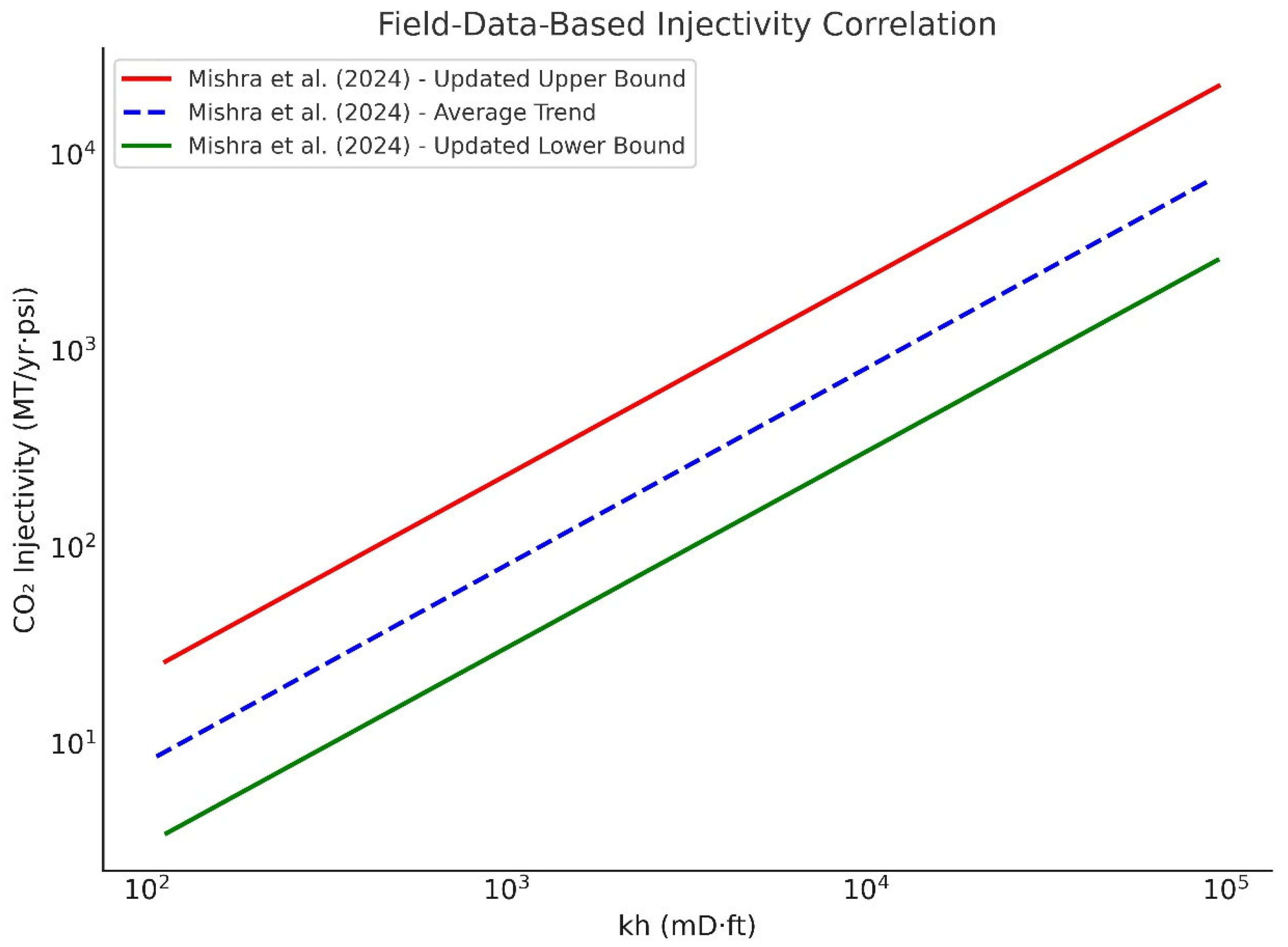
Mishra et al. [39] developed a field data-based correlation, building on an earlier work by Valluri et al. [17], to estimate the CO2 injectivity index using field data from large-scale storage projects. The approach provides a physically meaningful yet computationally simple means of assessing the injection potential of saline aquifers. It was derived from data covering nine major CO2 injection sites worldwide including Ketzin, IBDP, Snohvit, Nagaoka, SECARB, Aquistore, the MRCSP sites in Michigan and Kentucky, and AEP Mountaineer, spanning a wide range of depths (2000–10,000 ft), porosities (5–26%), and permeability-thickness ( k h ) values (hundreds to ≈ 60,000 mDft). Injection rates ranged from a few tens to over 2000 MT/day, ensuring representation across both pilot and industrial-scale operations. When the injectivity index ( J ) was plotted against k h on a log–log scale, a strong linear relationship emerged as seen in Figure 3. From this trend, three bounding relationships were defined to represent field variability: updated lower bound, J = 0.03 k h ; average trend, J = 0.08 k h ; updated upper bound, J = 0.23 k h .
These bounds form an empirical injectivity envelope; the upper trend corresponds to laterally continuous, high-quality sandstones (e.g., Mount Simon and Tubåen formations), while the lower bound represents more restrictive systems such as dolomitic or shaly intervals. The middle line ( J = 0.08 k h ) serves as a practical “best-estimate” correlation for typical saline aquifers. The correlation’s (Method A) strength lies in its field-based simplicity and dual applicability. In its forward form, it enables quick injectivity estimates when k h is known; in its inverse form, it allows k h to be inferred from measured injectivity. This makes it especially valuable during early site screening when detailed data are limited. To improve site-specific accuracy, Mishra et al. [39] introduced an analog refinement workflow based on Gower’s distance, which links target reservoirs to statistically similar field cases. Although Method A focuses solely on k h and thus omits effects of heterogeneity, anisotropy, and multiphase flow, it remains an effective first-order tool for evaluating injection potential. Its linear J - k h relationship reflects the central role of transmissibility in CO2 storage systems and serves as a benchmark for validating predictive models; a model that falls within this empirical envelope can be considered both physically realistic and consistent with observed field performance.

3. Results and Discussion

This section presents the outcomes of the integrated modeling framework developed to evaluate CO2 injectivity in the Entrada Sandstone of the San Juan Basin. The results are presented and discussed to reflect the sequential workflow established in this study. It begins with the model calibration and predictive simulation, which establish the baseline reservoir behavior under CO2 injection. This is followed by the sensitivity analysis, which examines the influence of key geological, fluid, and operational parameters on injectivity performance. Finally, the machine learning proxy development section will summarize the construction, validation, and comparative performance of the predictive models used to generalize injectivity responses across multiple scenarios. Together, these results form the basis for interpreting reservoir performance, evaluating model reliability, and developing data-driven strategies for CO2 storage site screening and optimization.

3.1. Simulating CO2 Injection Dynamics: From Calibration to Forecast

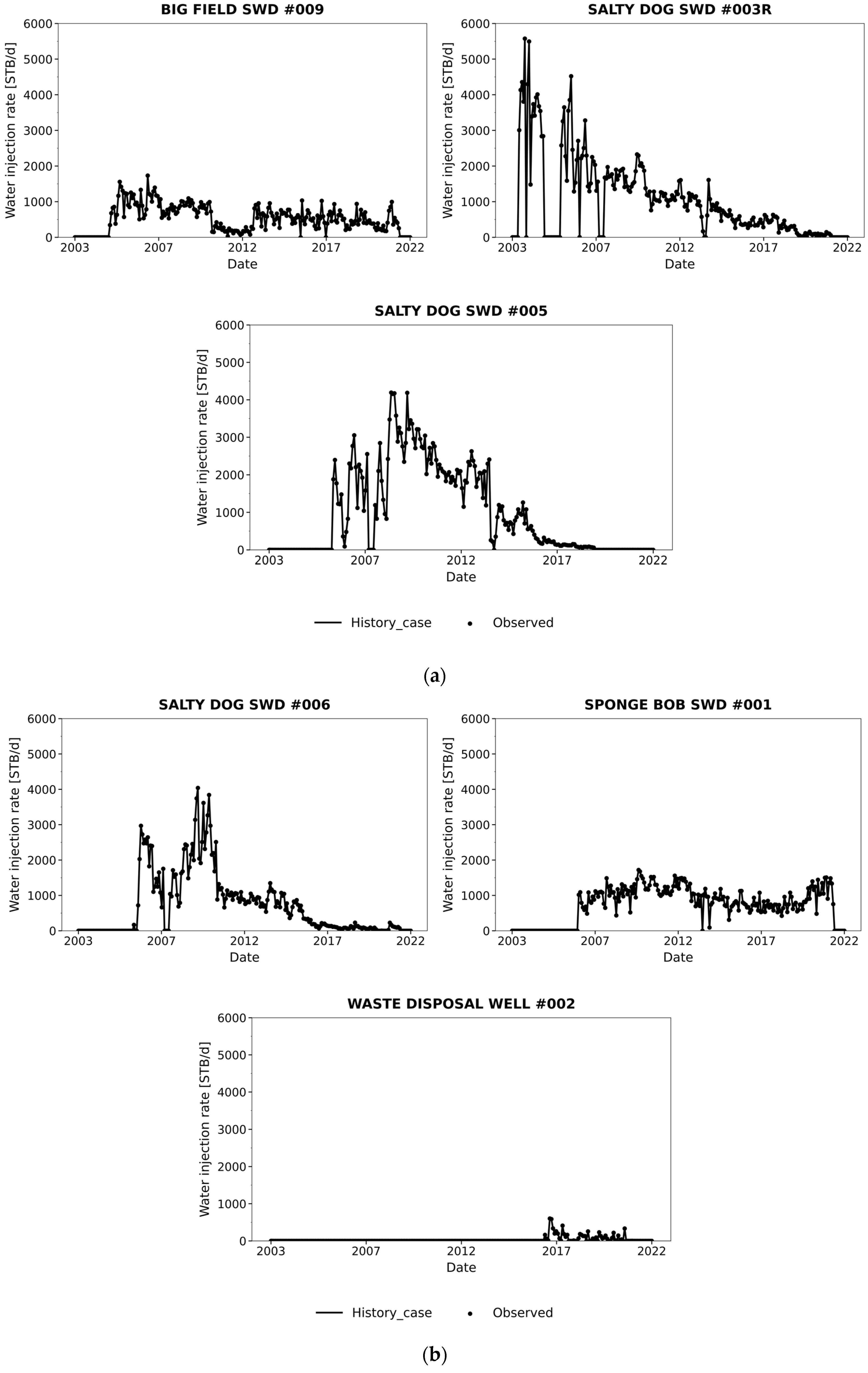
The calibrated hydrodynamic model achieved an overall history-match error of approximately 9.6%, demonstrating good agreement between simulated and observed field data [40]. Because water injection rates were imposed as boundary constraints, they were reproduced almost exactly by the simulator as shown in Figure 4, making bottomhole pressure (BHP) the main indicator of match quality.
As shown in Figure 5, the model successfully replicates the general pressure behavior across all six disposal wells throughout the injection period. Minor deviations are observed in some wells, particularly the Salty Dog wells, during short intervals where field measurements fluctuate or data gaps exist. These small discrepancies likely result from transient operational events such as pump interruptions or surface facility shutdowns that are not represented in the model. Despite these differences, the overall agreement confirms that the reservoir’s transmissibility and pressure-support mechanisms are well captured. The use of localized permeability multipliers proved effective in improving the match while preserving geological plausibility, indicating that moderate heterogeneity adjustments were sufficient to reproduce field conditions realistically. The resulting calibrated model provides a reliable foundation for predictive simulations, having captured the essential pressure-rate dynamics governing the Entrada Formation’s injection performance.
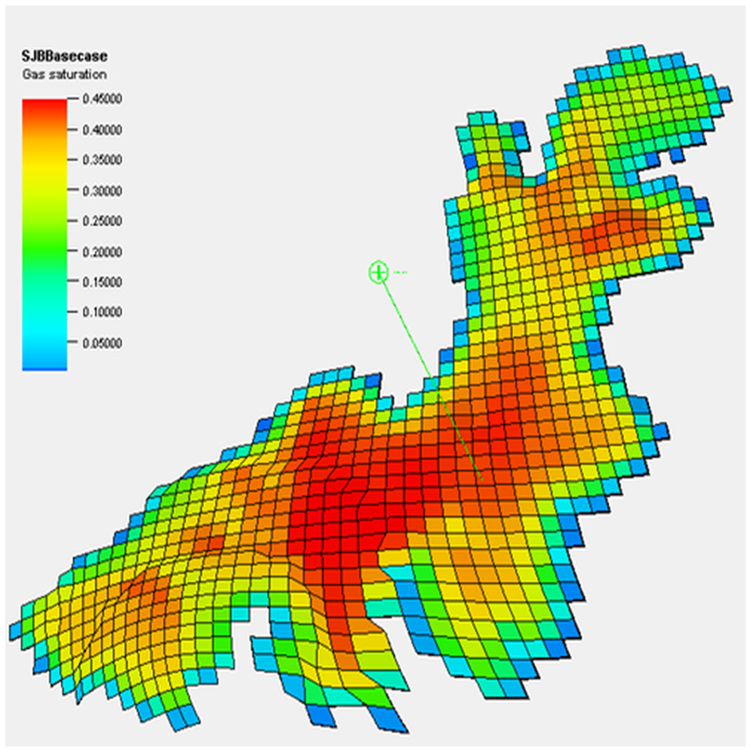
Using the history-matched model, a base case CO2 injection scenario was simulated for a 30-year forecast period. Figure 6 presents the simulated CO2 saturation distribution at the end of injection. Saturation values range from near zero (blue) to a maximum of about 0.45 (red) near the injection well. The plume exhibits an elongated geometry that follows high-permeability pathways, illustrating how reservoir heterogeneity strongly governs CO2 migration [41]. Lower-permeability zones provide lateral confinement, promoting localized accumulation and enhancing containment [42]. This pattern reflects the combined influence of permeability architecture and flow anisotropy on storage distribution.
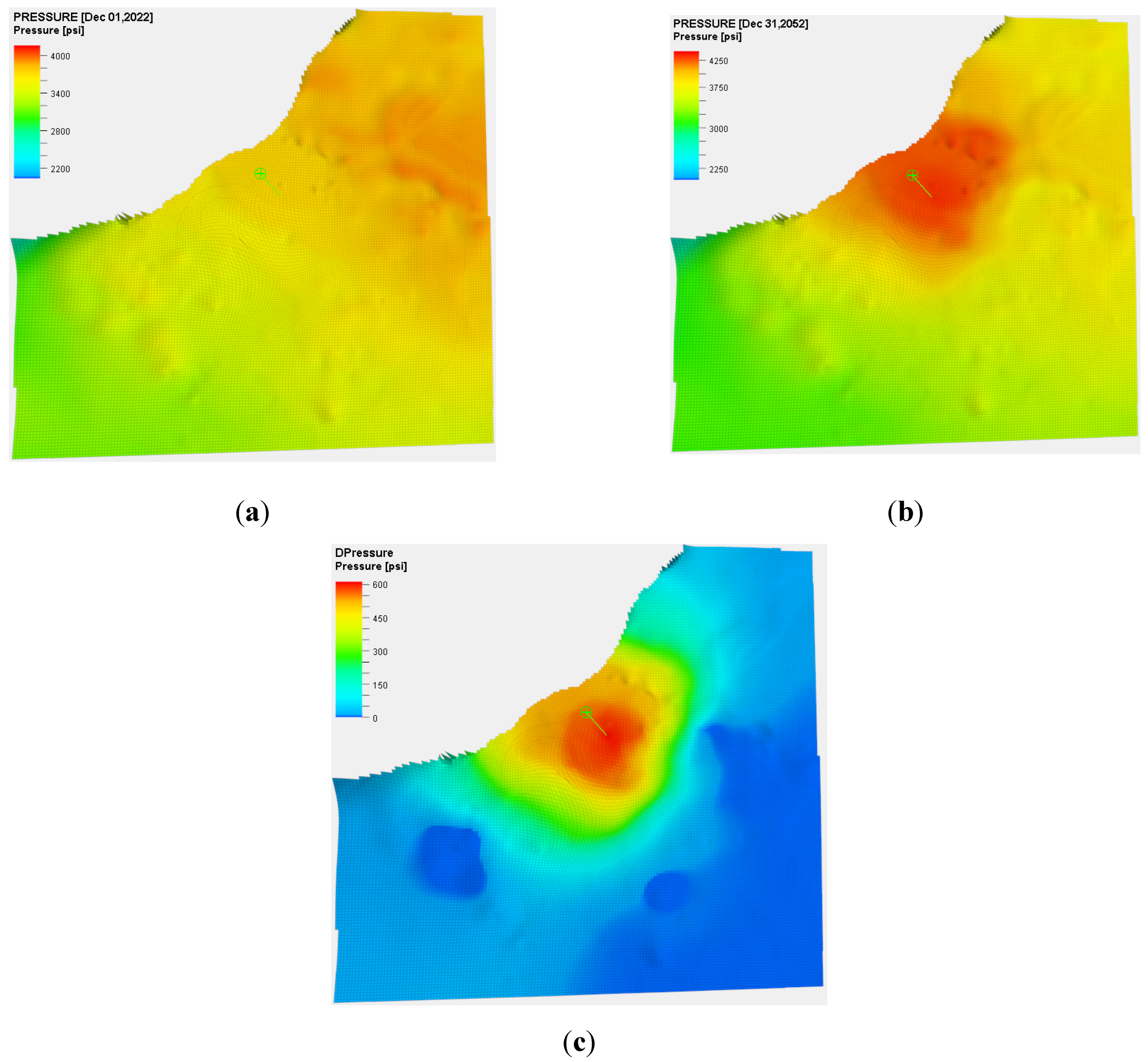
The pressure distribution after CO2 injection, shown in Figure 7, ranges from roughly 2200 psi at the periphery to 4500 psi near the wellbore with a maximum change of about 600 psi near the wellbore at the end of injection. The radial pressure gradient indicates that the system maintains a stable response, with localized buildup close to the injector and gradual dissipation outward. No abnormal overpressuring was observed beyond the immediate injection zone, suggesting that reservoir integrity is preserved and that the formation can safely accommodate the injection rate within operational limits.
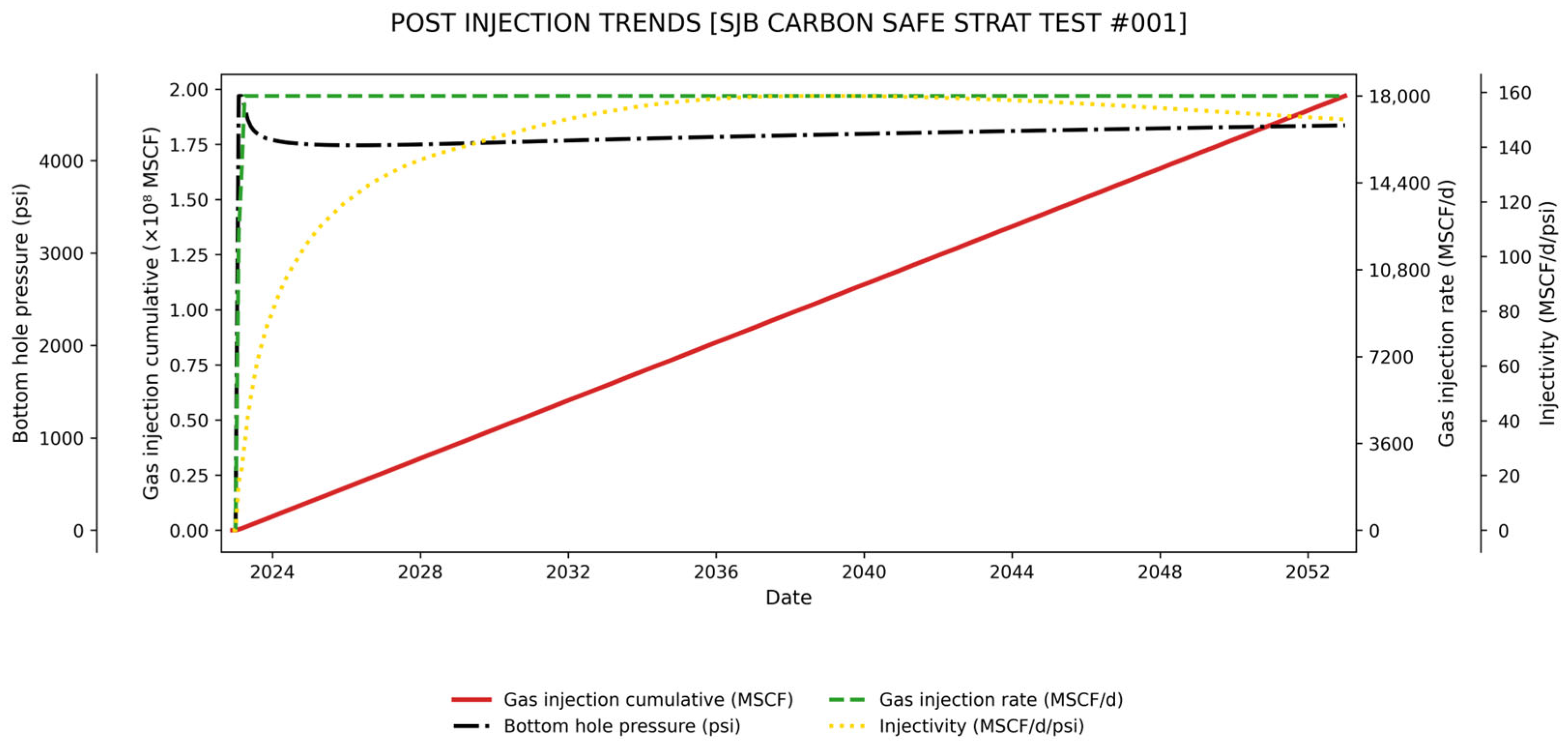
Figure 8 summarizes the base case performance trends for bottomhole pressure (black solid line), gas injection rate (red solid line), injectivity index (green solid line), and cumulative injected volume (red dotted line). During early injection, BHP rises rapidly to about 4700 psi, reflecting near-wellbore pressure buildup as CO2 displaces formation brine. The pressure then declines to around 4150 psi by mid-2029, marking reservoir adjustment as the injected CO2 redistributes and the pressure stabilizes. Thereafter, the pressure gradually increases to about 4350 psi, indicating a new equilibrium as continuous injection proceeds. The injection rate builds steadily until reaching the operational limit of 18 MMSCF/day, remaining below the fracture pressure constraint throughout the simulation. The injectivity index improves as the system stabilizes but begins to decline slightly after 2040, likely due to gradual pressure buildup and reduced effective permeability caused by ongoing CO2–rock interactions. Cumulative CO2 injection increases linearly over the forecast period, reaching roughly 200 MMSCF after 30 years, confirming that the reservoir can sustain long-term injection at the design rate without exceeding pressure constraints.

3.2. Parameter Ranking via Multi-Parameter Sensitivity

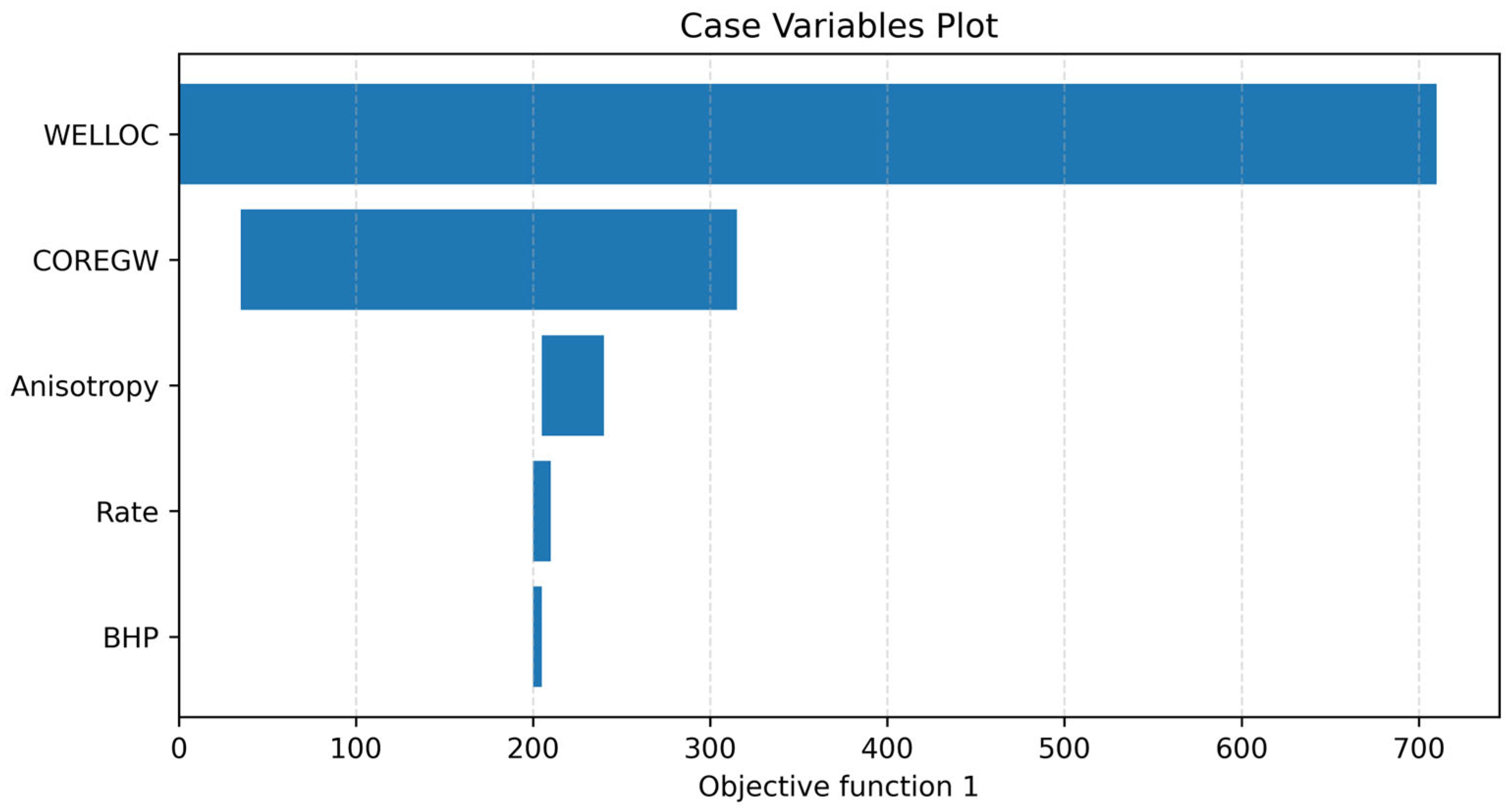
The sensitivity analysis integrated geological, petrophysical, and operational parameters to quantify their influence on CO2 injectivity and plume dynamics in the Entrada Sandstone. The combined results, summarized in Figure 9, rank the five most influential parameters in controlling injectivity responses: the effective k h defined by well locations (WELLOC) and df/ds, represented by the Corey exponents (COREYGW), emerged as dominant, followed by permeability anisotropy, while BHP and injection rate exerted comparatively minor effects. This ranking confirms that geological heterogeneity and relative permeability behavior govern injectivity far more strongly than operational parameters which are largely dependent on these influential factors.
Well locations which defined the effective k h were found to be the single most influential factor. Locations with higher k h values produced larger CO2 plumes and greater injectivity due to increased transmissibility [43]. However, these zones, an example as seen in Figure 6, exhibited more complex plume geometries, often elongated and irregular, reflecting preferential flow through high-permeability channels. When coupled with high VDP > 0.55, these areas showed pronounced channeling and fingering, underscoring how heterogeneity amplifies plume irregularity. In contrast, lower k h regions generated smaller, more stable plumes that advanced uniformly, offering improved containment but reduced injectivity [44].
The second-most significant control, df/ds, derived from Corey gas and water exponents, captured the interaction between CO2 and brine at the displacement front [45]. Low Corey exponents produce steep fractional flow curves, indicating abrupt saturation transitions and rapid CO2 displacement [46]. These conditions favor higher instantaneous injectivity but increase the likelihood of fingering and uneven plume advance. Higher exponents yield gentler slopes and smoother saturation changes, leading to steadier, more predictable CO2 fronts. Permeability anisotropy ranked next in influence, impacting the directional spread of CO2. High anisotropy (where horizontal permeability exceeds vertical) produced wide but shallow plumes, enhancing lateral sweep while limiting vertical migration [47]. Low anisotropy encouraged balanced plume development and improved containment, though with lower overall injectivity. The interplay between anisotropy and k h defined local flow patterns. High- k h , high-anisotropy zones favored rapid horizontal expansion, while low- k h , low-anisotropy zones supported slower but more stable movement. By contrast, BHP and injection rate ranked lowest in Figure 9 tornado plot. Although higher values increased near-wellbore pressure and short-term injectivity, they did not significantly alter overall plume geometry or storage distribution. These operational parameters act mainly as modulators within geological constraints, important for maintaining safe injection pressures but not for controlling flow pathways.

3.3. Data Foundation and Statistical Diagnostics

The dataset used for this analysis comprised 390 simulation combinations from the dominant parameters generated through Latin hypercube sampling within realistic parameter ranges. Prior to modeling, diagnostic evaluations were performed on each predictor (X1X4) and the target variable (Y). X1 is the VDP, X2 represents the permeability anisotropy, X3 is df/ds, X4 is the k h , while Y is the CO2 injectivity. The goal was to identify distributional irregularities, potential outliers, and relationships among variables that could influence model stability and predictive performance.
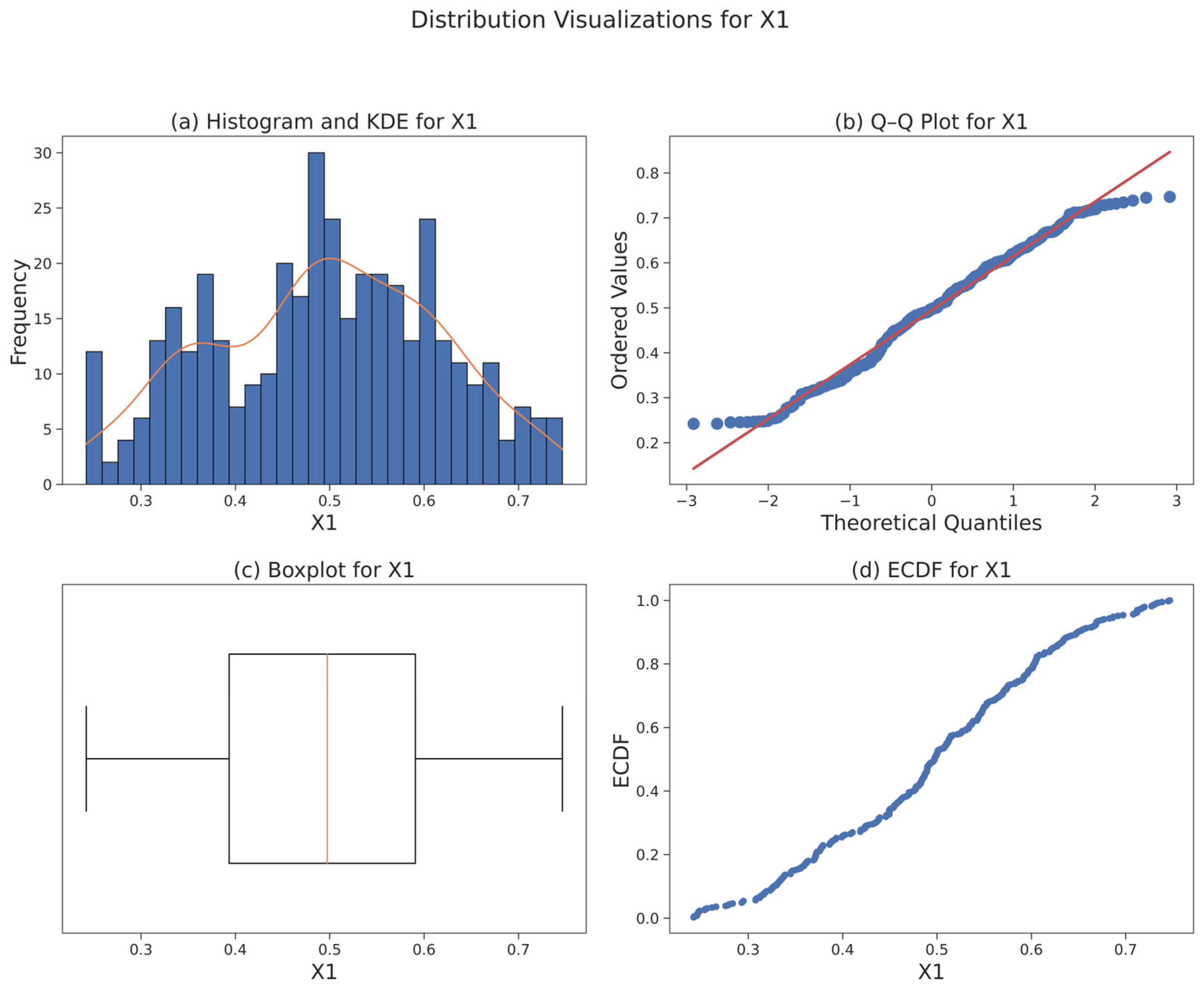
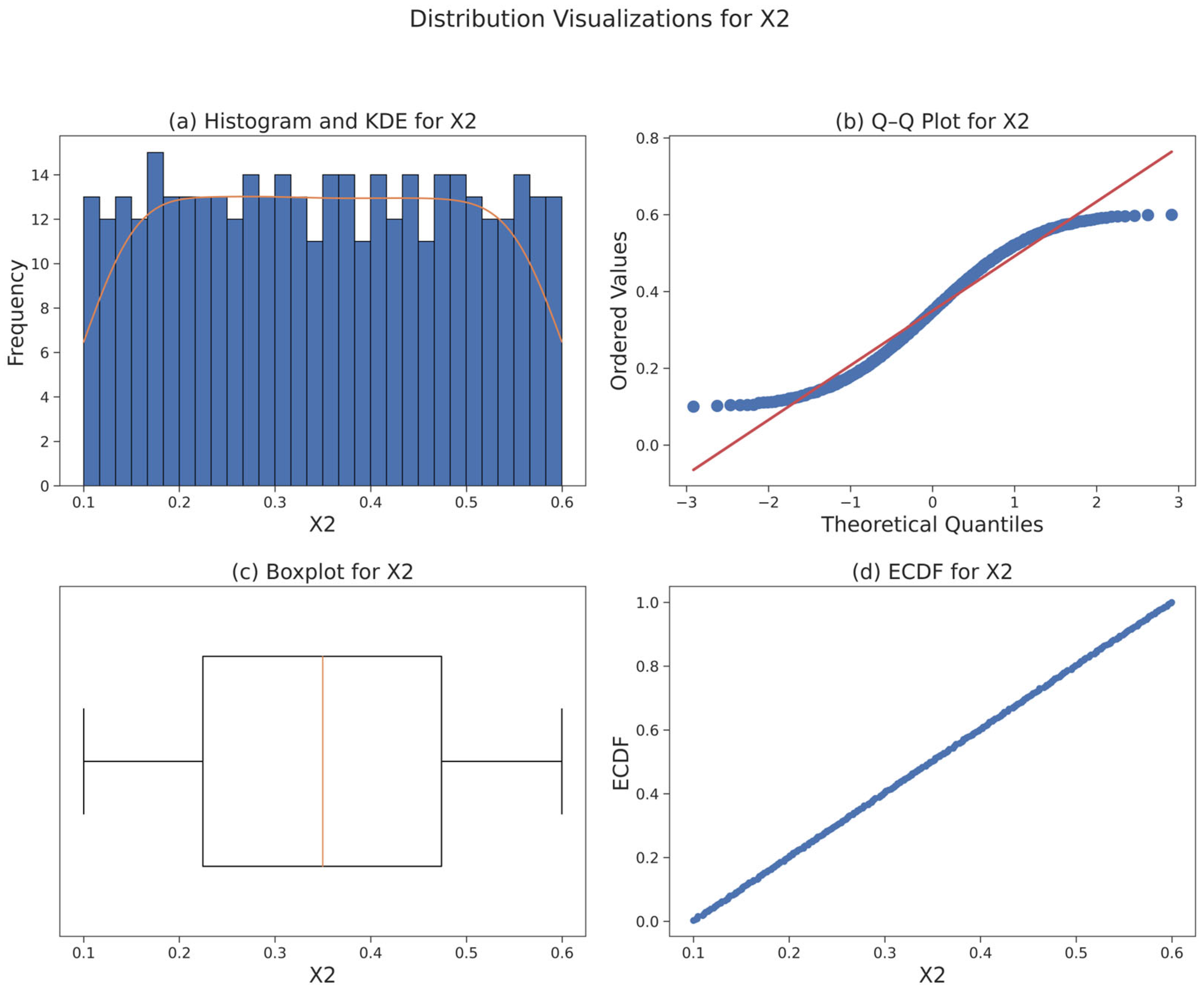
The univariate distribution diagnostics collectively convey a consistent and interpretable pattern. X1 displays a mean of 0.494 with a standard deviation of 0.121, suggesting moderate variability around its center. The nearly zero skewness (−0.10) confirms a balanced distribution, while the slightly negative kurtosis (−0.72) points to lighter tails relative to the normal curve [48]. In Figure 10, the histogram shows a smooth, gently peaked form, and the Q–Q plot follows the reference line closely except for mild deviations at the extremes. The boxplot and Empirical Cumulative Distribution Function (ECDF) further indicate a well-distributed dataset, with a symmetric spread and the gradual S-shaped ascent typical of a near-normal variable [48]. X2 presents an even more uniform profile. With a mean of 0.350, standard deviation of 0.144, and almost zero skew (0.01), the distribution is essentially flat, consistent with its negative kurtosis (−1.20). The visual diagnostics in Figure 11 reinforce this interpretation: the histogram lacks any pronounced central tendency, the ECDF is almost linear, and the Q–Q plot exhibits the gentle S curve expected when a uniform distribution is compared to a normal reference [48].
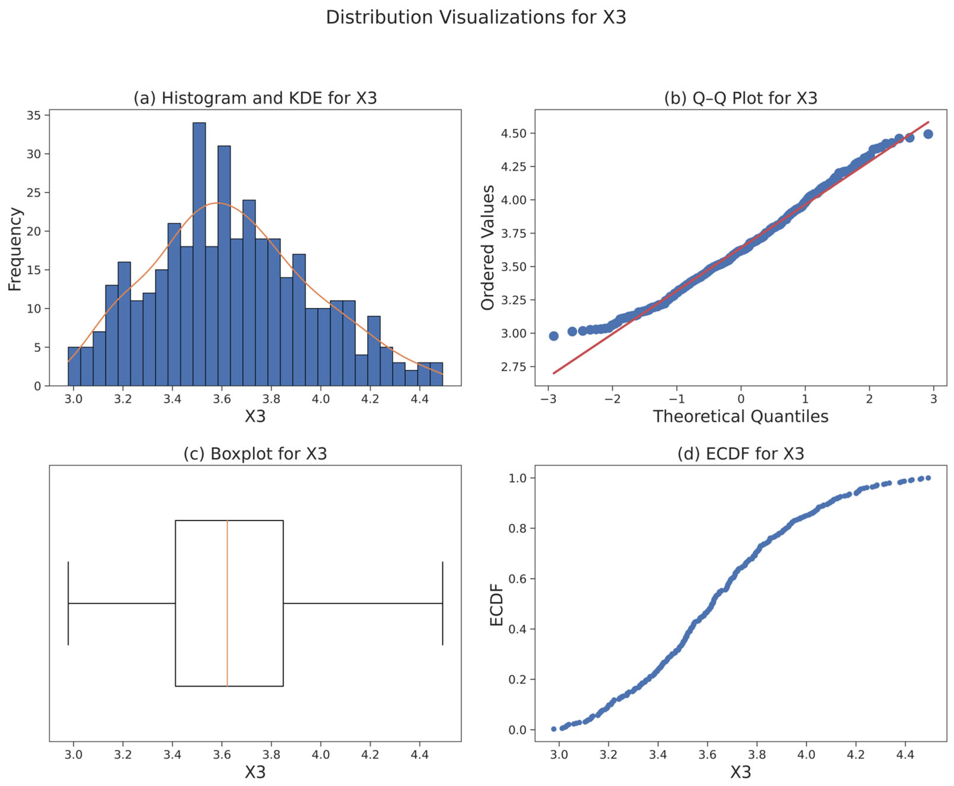
X3 occupies a middle ground between the first two variables. It has a mean of 3.641 and standard deviation of 0.323, accompanied by a mild positive skew (0.30) and slightly negative kurtosis (−0.38). As shown in Figure 12, the histogram is broadly symmetric, and the Q–Q plot is nearly linear apart from modest curvature near the tails. The boxplot suggests a compact and balanced spread without any influential observations [48]. These diagnostics indicate that X1, X2, and X3 are statistically well-behaved, largely symmetric, devoid of extreme outliers, and suitable for subsequent modeling analyses without further engineering.
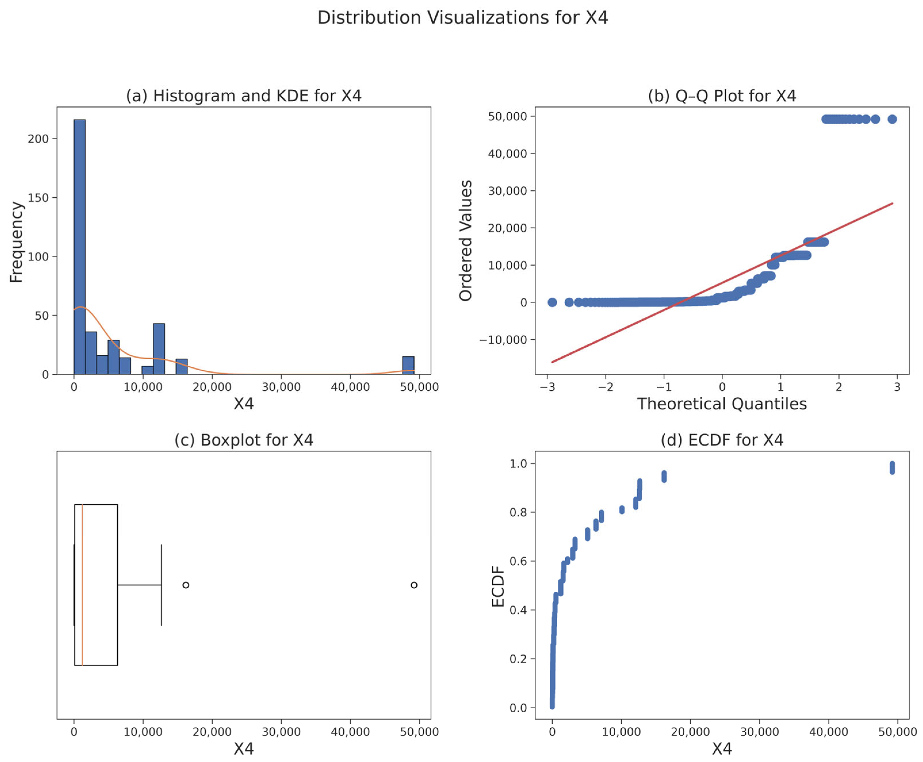
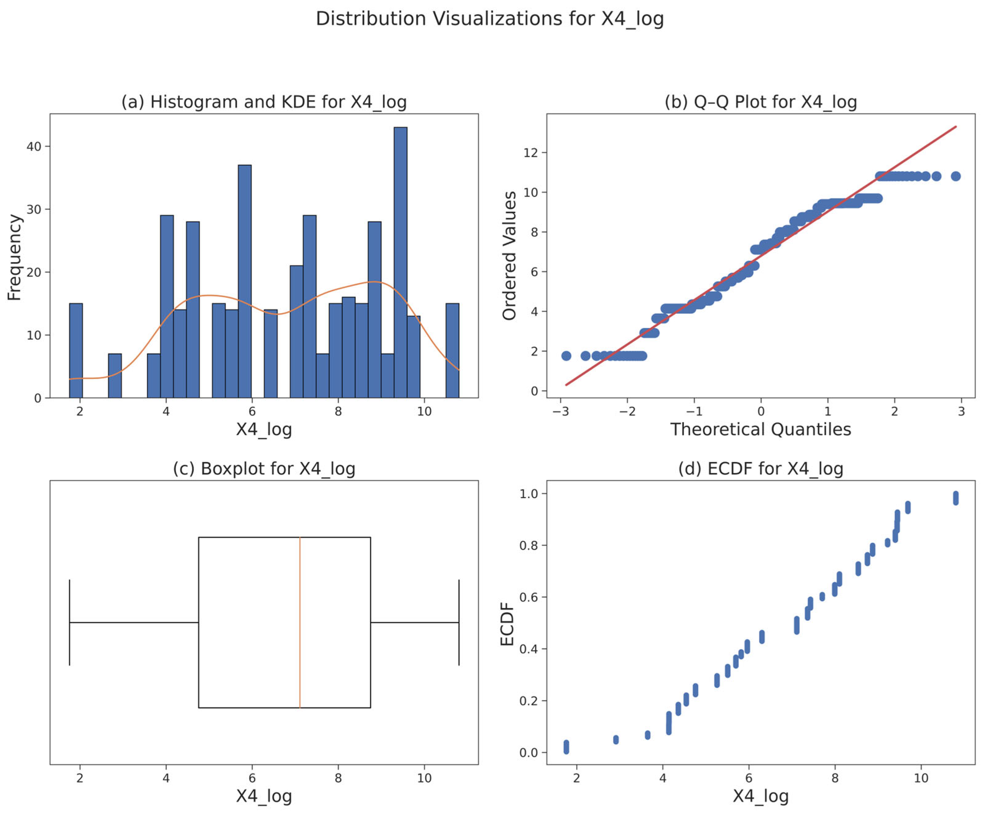
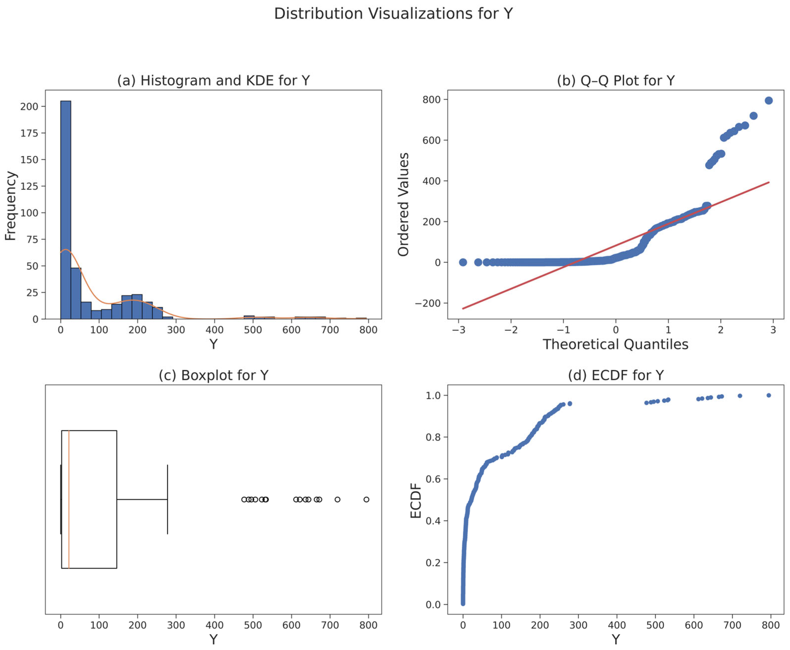
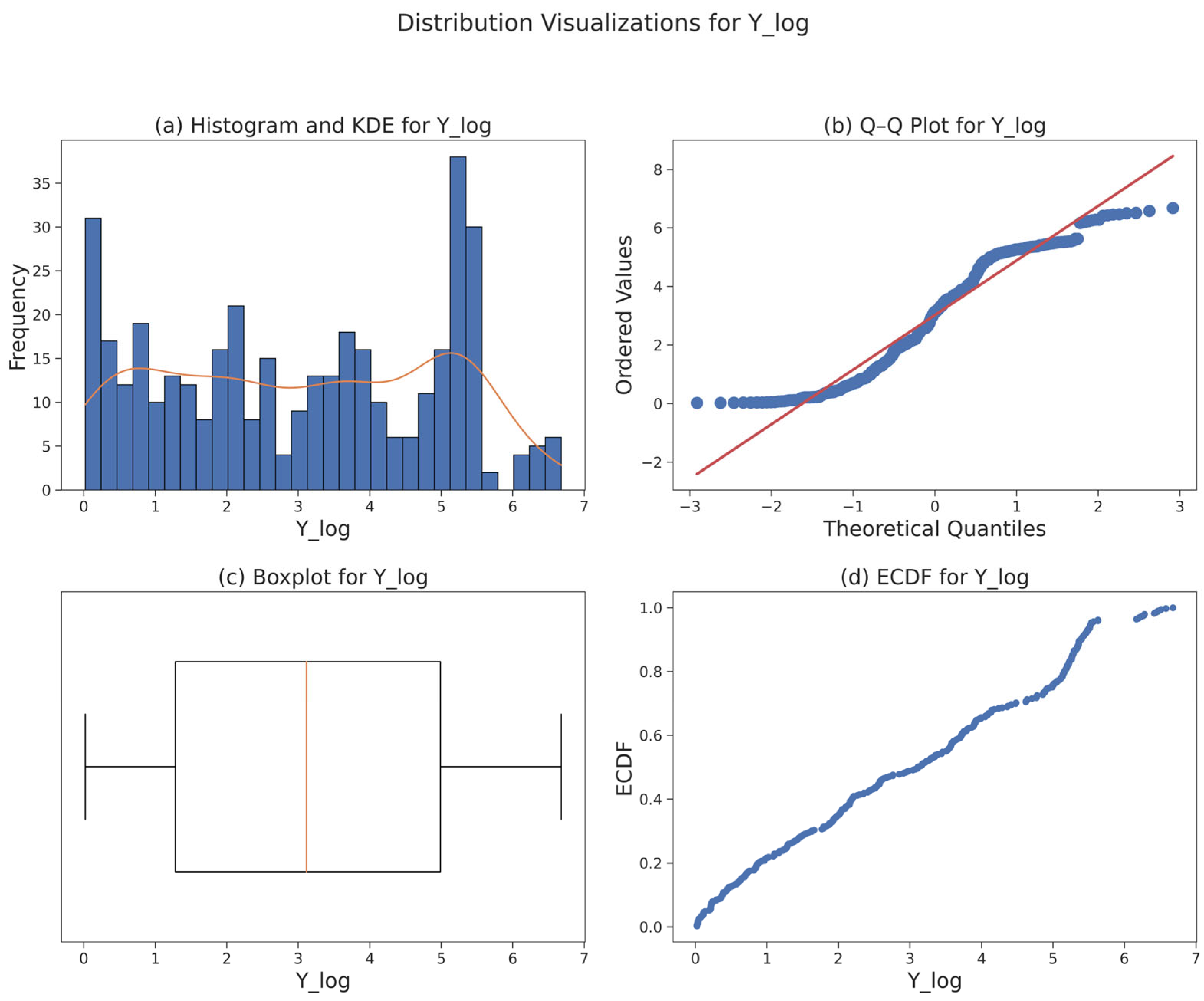
By contrast, the distribution of X4 as seen in Figure 13, displayed a pronounced right skew (skewness = 3.36) and heavy-tailed distribution (kurtosis = 11.96), dominated by numerous small values and a few extremely large ones. Such imbalance introduces heteroscedasticity and leverage effects that can distort model coefficients [49]. To correct this, a logarithmic transformation is applied, yielding a more symmetric distribution (skewness ≈ −0.23, kurtosis ≈ −0.84) and stabilized variance which is visualized in Figure 14 [50]. The response variable, Y, exhibited a similar right-skewed pattern, with high variance and multiple outliers as visualized in Figure 15. Applying the transformation Ylog = log (1 + Y) significantly improved its symmetry and reduced tail weight as illustrated in Figure 16 [50], making it more compatible with both linear and nonlinear learners. These transformations collectively regularized the dataset and mitigated the impact of extreme observations.
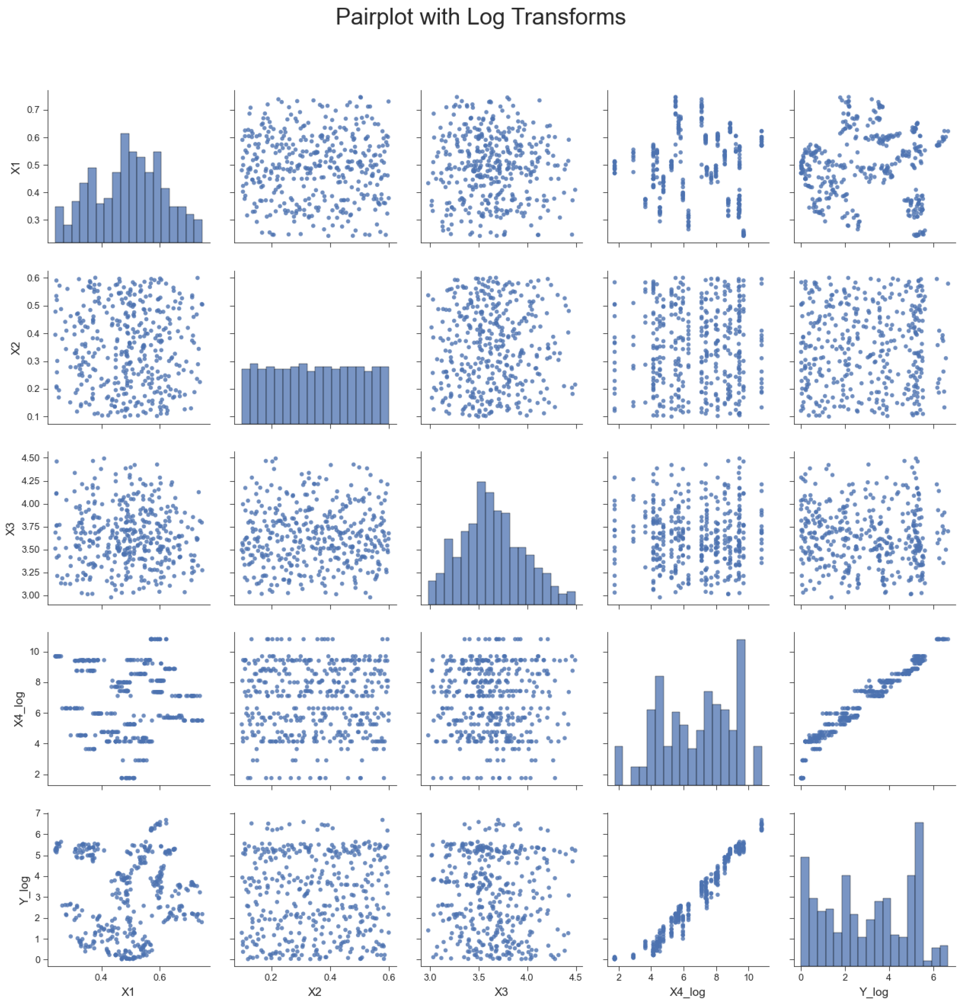
Bivariate analysis after applying log transformations in Figure 17 shows the relationship between log-transformed X4 and Y become almost linear. The remaining predictors show modest secondary correlations, implying that they contribute incrementally but do not have a dominant predictive value. From a modeling standpoint, these diagnostics indicate that X4, representing the permeability-thickness term, is the principal driver of injectivity, while X1X3 provide complementary adjustments that refine model accuracy. Working in the logarithmic domain for X4 and Y not only stabilizes residual variance but also enhances interpretability and numerical robustness [51]. This approach maintains compatibility with both regression-based and ensemble methods, as the transformation regularizes the feature space without distorting the physical meaning [52]. Using log (1 + Y) instead of log(Y) preserves information for low-value data points, ensuring resilience for near-zero injectivity values.

3.4. Comparative Evaluation of Machine Learning Models for CO2 Injectivity

This section presents the results of the machine learning models developed to predict the CO2 injectivity index. The objective is to determine which algorithm most effectively captures the relationships between the parameters governing injectivity. The analysis follows an optimization of the individual models across different data splits for training and testing to assess performance stability while validating the final models using both the held-out and blind dataset to evaluate generalization.
The impact of the train–test split ratio on predictive performance is summarized in Table 1 and Table 2. Across all models, the regularized regressors, Ridge, Lasso, and ElasticNet, along with Random Forest consistently achieved high R2 values (≈0.97–0.99), indicating robust performance regardless of data partitioning. XGBoost maintained strong results up to a 30% test size before showing minor degradation, whereas LightGBM exhibited greater sensitivity at larger test sizes. Response Surface deteriorated rapidly, producing negative R2 values beyond 20%, confirming its limited reliability for this dataset division. The negative R2 values reflect poor predictive performance and this occurs when a model performs worse than a baseline predictor that uses the mean of the observed data [53]. As the test size increases and the available training data decrease, the model fails to generalize and produces large prediction errors, leading to the negative R2 values. The aggregate metrics in Table 2 show that the 10% test split provides the most stable and accurate results, yielding a mean R2 of 0.96 with the lowest overall error. Beyond this threshold, the models became more variable, with the average R2 dropping sharply due to instability in the Response Surface predictions. Based on this observation, the 0.9/0.1 split was selected for all subsequent analyses to preserve both accuracy and consistency.
With the data partition finalized, the next stage focused on evaluating the comparative performance of multiple machine learning algorithms in predicting CO2 injectivity. Seven machine learning models were trained and tested and performance metrics which included the mean squared error (MSE), mean absolute error (MAE), and coefficient of determination (R2) for both training and testing datasets. Table 3 summarizes these results. From Table 3, the Lasso regression model produced the weakest overall performance, characterized by high test errors (MSE = 1211.45; MAE = 16.07) and a relatively low test R2 = 0.958. Its excessive penalization likely over-simplified the model, erasing useful variance in the data [54]. The LightGBM model performed marginally better at a test R2 of 0.965, though it exhibited instability during prediction, with noticeably inflated test errors (MSE = 1010.74; MAE = 15.68). Similarly, the Response Surface approach demonstrated acceptable training accuracy but failed to properly generalize, showing a sharp rise in test MSE = 872.50 and MAE = 18.74, with R2 = 0.970. These three models, while computationally tractable, proved less robust for the relatively small and noise-sensitive dataset.
ElasticNet regression, which balances L1 and L2 regularization [55], offered modest improvement (test R2 = 0.971). However, its elevated test MSE = 851.04 and MAE = 13.61 indicated that the model did not fully reconcile bias and variance, performing less consistently across different subsets of data. The XGBoost model, a tree-based gradient boosting algorithm, delivered stronger accuracy with a test R2 = 0.993 and low MAE = 5.43, though its MSE = 187.51 revealed mild overfitting relative to its training performance. In contrast, Random Forest maintained more consistent generalization, achieving a comparable R2 = 0.994 but with higher absolute error (MAE = 7.56). Both ensemble models achieved strong results, yet their interpretability and reproducibility were limited compared to their linear counterparts. Amid these high-performing models, the Ridge regression model emerged as the most balanced and analytically transparent choice. Despite a slightly higher test MSE = 175.60 relative to Random Forest, Ridge achieved a matching R2 = 0.994 and the lowest test MAE = 7.35 among the linear models. Its stability, combined with a clear mathematical formulation, makes it particularly suitable for CO2 injectivity analysis, where physical interpretability is as important as predictive strength.
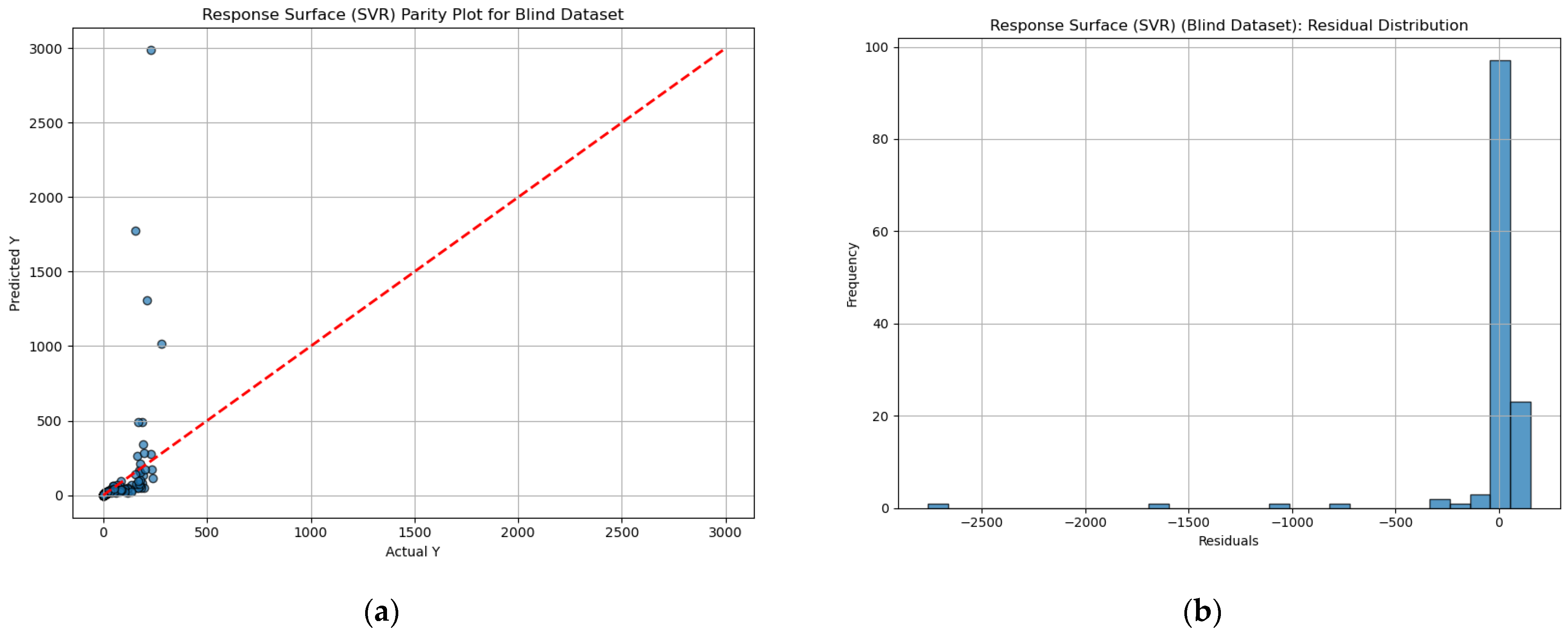
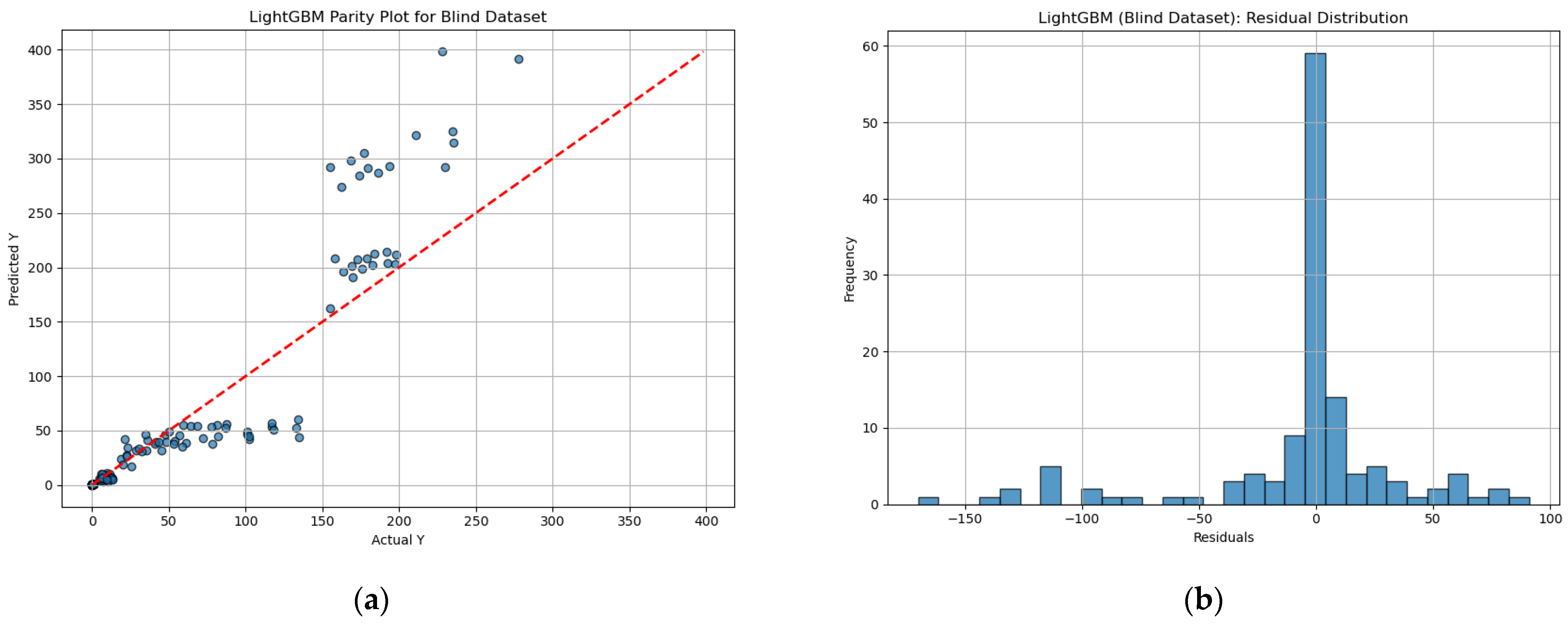
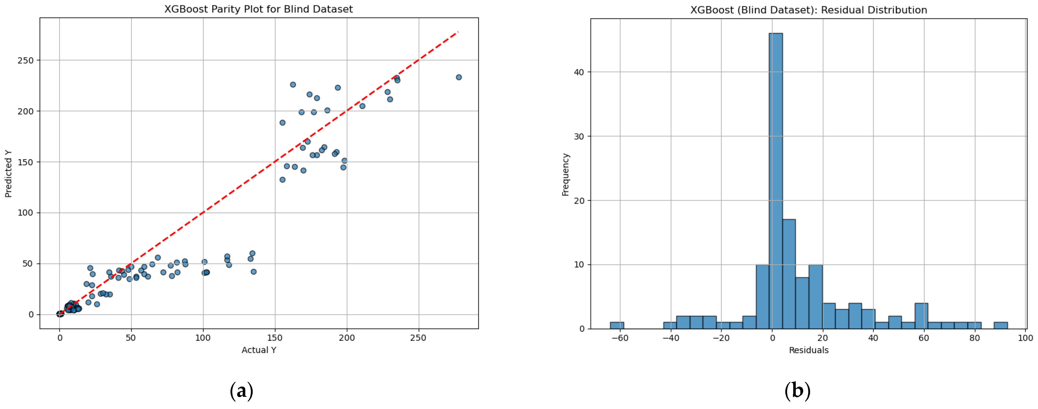
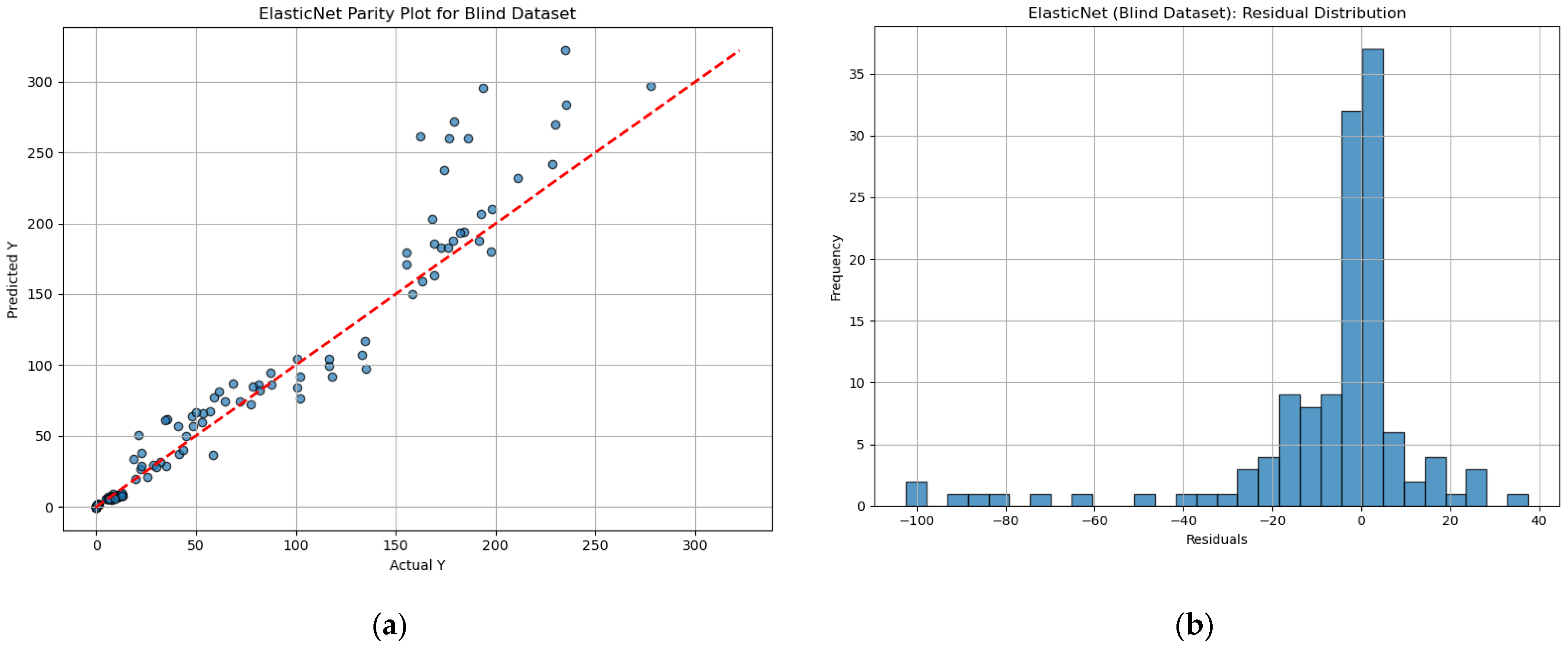
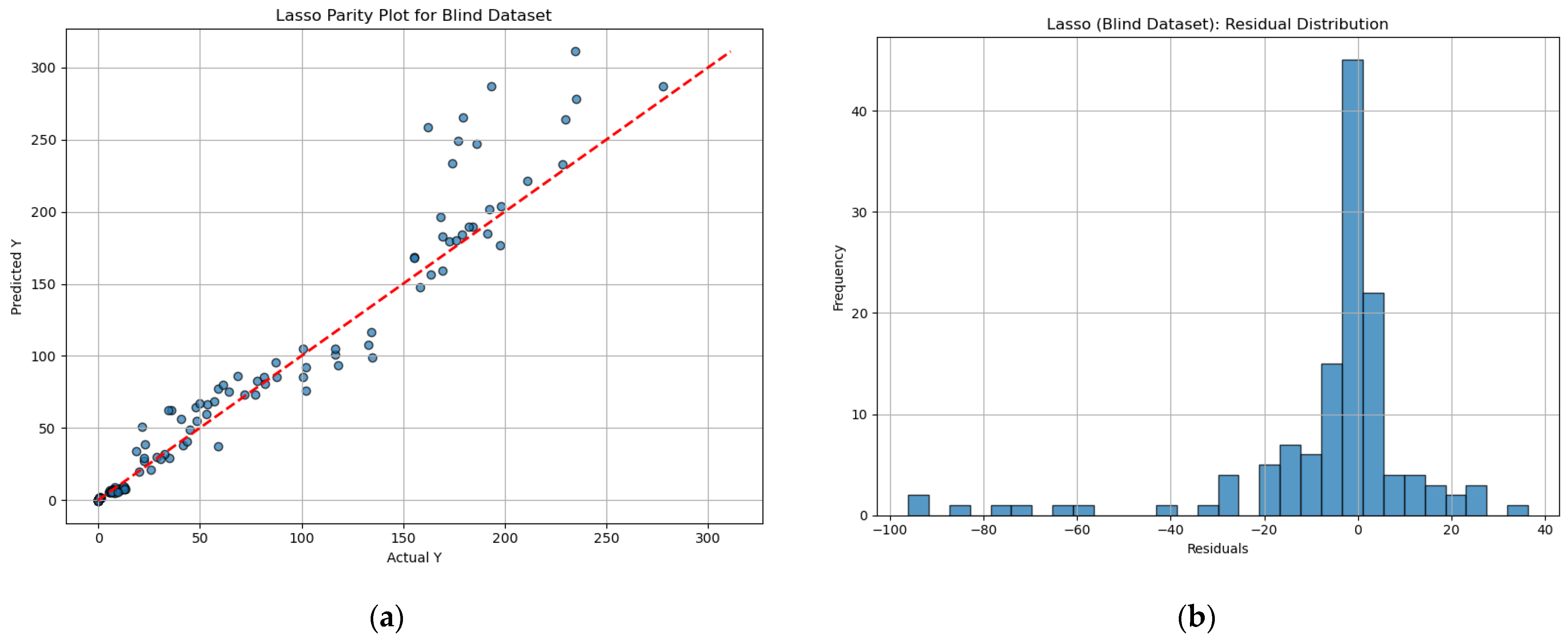
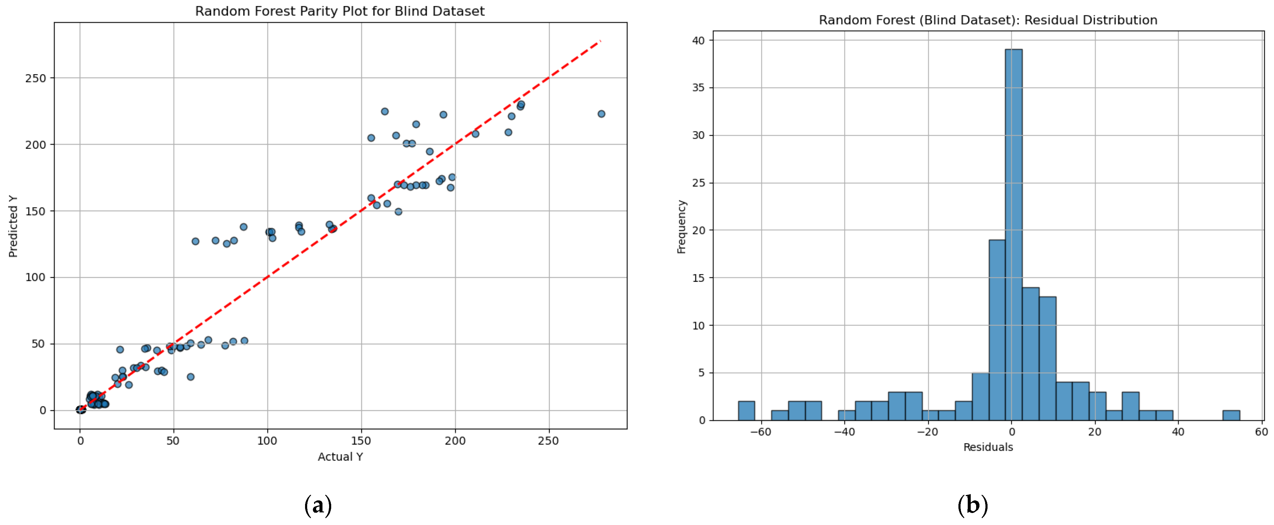
Following the train–test evaluation, a blind dataset, completely excluded from the model calibration process, was used to test the generalization capability of each algorithm. This stage provides a realistic assessment of how well the models perform when exposed to new data, independent of any patterns learned during training. Figure 18, Figure 19, Figure 20, Figure 21, Figure 22, Figure 23 and Figure 24 present the parity plots and residual distributions for all models in this study, while Table 4 summarizes their numerical performance metrics.
The Response Surface model in Figure 18 showed the poorest performance overall. Most of its predictions cluster tightly at the lower end, with several extreme outliers. This indicates that the model was unable to scale its predictions effectively across the injectivity range. The residual plot further confirms this, displaying a heavily skewed and dispersed pattern that points to systematic underestimation of high injectivity values leading to an extremely high blind MSE (95,860.72) and a negative R2 value of −0.16. The LightGBM model in Figure 19 produced more stable results, especially for moderate injectivity values, but its predictions became scattered toward the upper range. Its blind MSE reached 1901.12, with a relatively large MAE of 23.82 and a weak R2 of 0.66. While the residuals peak sharply around zero, their long tails suggest inconsistent fitting and a tendency to overfit localized regions within the dataset.
Figure 20 shows that the XGBoost model followed a similar trend but with slightly improved alignment along the 1:1 line, achieving a blind R2 of 0.88 and smaller errors (MSE = 640.75; MAE = 15.43). Its predictions captured mid-range patterns reasonably well, although mild over-prediction persisted at higher injectivities. The residual distribution was narrower than LightGBM’s, implying better generalization but still some variability in the model’s higher-end behavior.
The ElasticNet model for injectivity is
Y = e x p [ 0.351672 + 3.43671 X 2 0.571783 X 3 + 0.00802503   l o g ( X 4 ) + 2.77931 X 1 2 0.104221 X 1 X 2 0.37867 X 1 X 3 0.669109 X 2 X 3 0.121797 X 2 l o g ( X 4 ) + 0.0699483 X 3 2 + 0.0101764 X 3 l o g ( X 4 ) + 0.0686511 ( l o g ( X 4 ) ) 2 ] 1
and the Lasso model for injectivity is
Y = e x p [ 0.527848 + 2.88966 X 2 0.0617713 X 3 + 2.46421 X 1 2 0.294785 X 1 X 3 + 0.00557158 X 1 l o g ( X 4 ) 0.556733 X 2 X 3 0.107523 X 2 l o g ( X 4 ) + 0.0726415 ( l o g ( X 4 ) ) 2 ] 1
where X1 is the Dykstra–Parsons coefficient (VDP), X2 represents the permeability anisotropy, X3 is the slope of fractional flow curve (df/ds), X4 is the permeability-thickness product ( k h in mDft), while Y is the CO2 injectivity in MSCF/day-psi.
In Figure 21 and Figure 22, the ElasticNet and Lasso models offered stable, interpretable, and moderately accurate results. The Lasso model achieved a blind R2 of 0.92 (MSE = 460.31; MAE = 10.97), while ElasticNet followed closely with R2 = 0.90 (MSE = 554.90; MAE = 12.03). Both models maintained compact, centered residuals and linear parity plots, capturing the overall pattern of injectivity variation with only minor underestimation at higher ends. Their functional forms in Equations 3 and 4 make it possible to interpret the influence of the four controlling parameters. Positive coefficients for X2 and log(X4) reflect their reinforcing effects on injectivity, while negative coefficients for X1 and X3 indicate their moderating influence. Interaction terms like X1X3 and X2log(X4) describe the coupled effects between reservoir uniformity and flow mobility.
Figure 23, which shows visualizations for the Random Forest model, suggests that it produced highly consistent predictions with a blind R2 of 0.93, the low MSE of 344.38, and low MAE of 11.17. The blind data points are tightly spread about the 45° line and the residual distribution centered mostly at or near zero. A few outliers appear at the upper edge, but the overall spread is small. This indicates strong generalization and robust predictive capacity across the dataset. Finally, the Ridge regression model in Figure 24 stood out as the most balanced among all. It performed comparably to Random Forest but with the added benefit of interpretability. The parity plot aligns very closely with the diagonal, showing excellent agreement between predicted and actual values at a blind R2 of 0.93 and acceptable low MSE and MAE of 410.54 and 11.03, respectively. Its residuals are sharply centered around zero with minimal dispersion, reflecting both precision and stability. What makes Ridge particularly appealing is that, despite being simpler than the ensemble models, it achieved nearly identical accuracy while keeping the coefficients explainable.
The functional form of the Ridge model clearly defines how each parameter affects injectivity as seen in
Y = e x p [ 2.61281 1.59397 X 1 + 5.08711 X 2 1.70957 X 3 + 0.0204346 l o g ( X 4 ) + 5.22806 X 1 2 0.661057 X 1 X 2 0.296364 X 1 X 3 0.196089 X 1 l o g ( X 4 ) 0.144468 X 2 2 0.925907 X 2 X 3 0.180602 X 2 l o g ( X 4 ) + 0.237071 X 3 2 0.00423331 X 3 l o g ( X 4 ) + 0.0796603 ( l o g ( X 4 ) ) 2 ] 1
where X1 is the Dykstra–Parsons coefficient (VDP), X2 represents the permeability anisotropy, X3 is the slope of fractional flow curve (df/ds), X4 is the permeability-thickness product ( k h in mDft), while Y is the CO2 injectivity in MSCF/day-psi.
In this expression, permeability anisotropy (X2) and permeability thickness (X4) exert strong positive effects, while higher heterogeneity (X1) and steeper fractional flow slopes (X3) inversely affect injectivity. The inclusion of quadratic and cross terms allows the Ridge model to capture nonlinear dependencies while maintaining a clear link to reservoir physics.
All together, the blind test results reveal a clear hierarchy of model performance to entirely unseen data. The ensemble methods delivered high accuracy but limited interpretability, while the Ridge regression achieved nearly identical predictive strength with full analytical transparency. Its well-balanced error metrics, stable residual behavior, and physically meaningful coefficients make Ridge the most reliable and interpretable model for predicting CO2 injectivity in heterogeneous formations like the Entrada which is the formation of interest in this study.

3.5. Bridging Data and Physics: Validating Ridge-Based CO2 Injectivity Predictions with Global Field Correlation

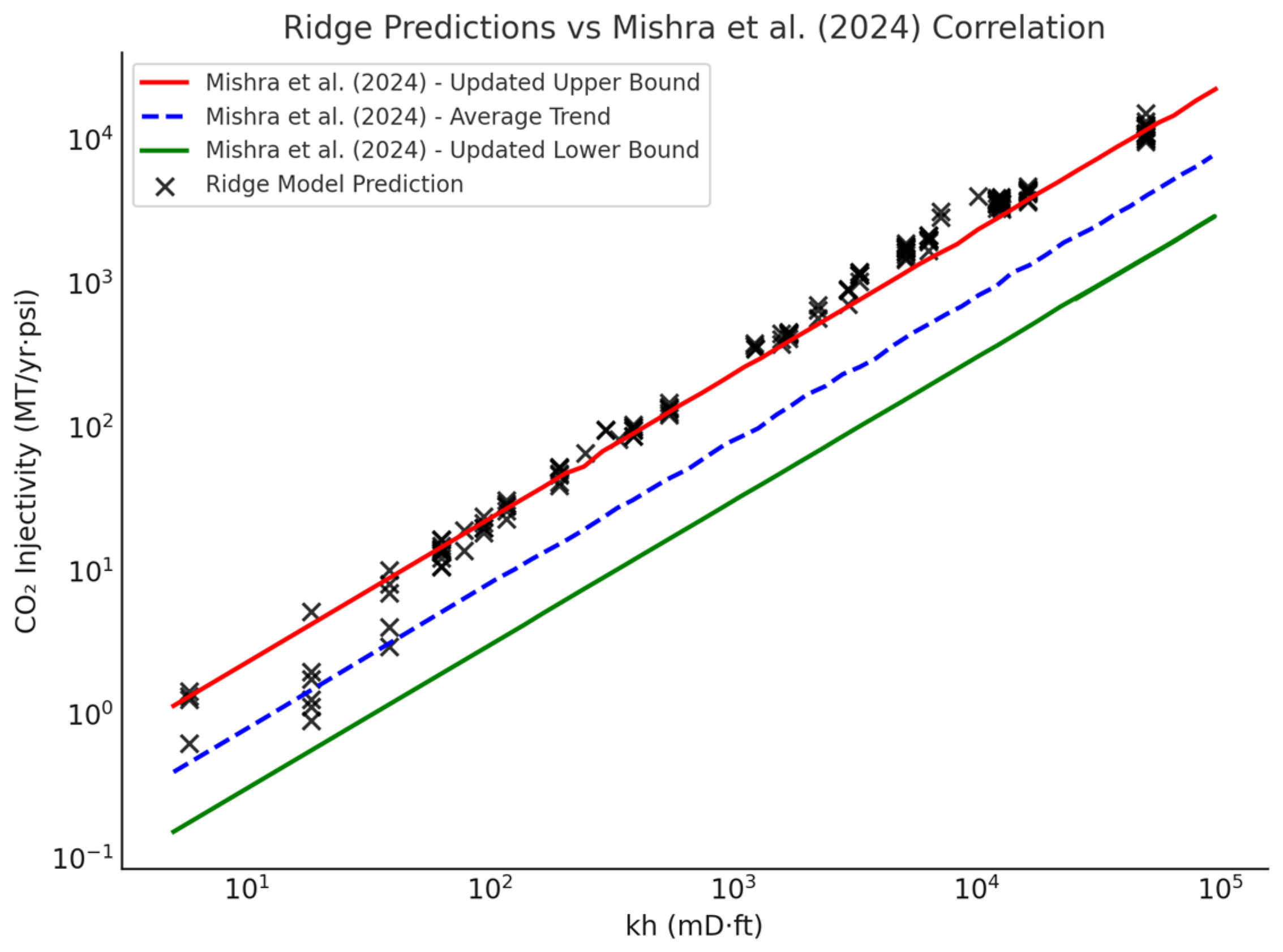
The blind test evaluation demonstrated that the Ridge regression model offered the best combination of accuracy, consistency, and interpretability among all algorithms tested. However, strong numerical performance alone does not ensure physical realism. To confirm that the model’s predictions align with the established field behavior, the Ridge model was validated against the empirical injectivity correlation (Method A) developed by Mishra et al. [39], previously described in the methodology. As outlined earlier, Method A provides a set of three field-derived linear trends relating the CO2 injectivity index ( J ) to the permeability-thickness product ( k h ). These trends define an injectivity envelope bounded by J = 0.03 k h (lower), J = 0.08 k h (average), and J = 0.23 k h (upper), which collectively capture the variability observed across multiple large-scale CO2 injection projects worldwide.
Figure 25 presents the comparison between the Ridge-predicted injectivity values for the Entrada Formation and the Mishra et al. [39] envelope. Both axes are plotted on logarithmic scales, with the blue dashed line representing the average trend ( J   = 0.08 k h ), the red and green lines marking the upper and lower bounds, and the black “×” symbols denoting the Ridge model predictions. The comparison shows a strong alignment between the Ridge results and the empirical field trends. The predicted values follow the same log-log proportionality and largely fall within the envelope defined by Mishra et al. [39]. Most points cluster near the upper bound, indicating that the Entrada Formation possesses high injectivity potential, consistent with a dominantly sandstone reservoir characterized by good lateral connectivity and strong pressure dissipation. A smaller portion of predictions lies near the average line, corresponding to moderately permeable zones where small variations in thickness or anisotropy reduce flow capacity. Only a few points approach the lower limit, suggesting that low-quality or poorly connected intervals are uncommon in the modeled domain. This spatial distribution agrees well with geological interpretations of the Entrada Formation. The close agreement between the Ridge-predicted values and Mishra et al. [39]’s empirical trends demonstrates that the model’s predictions are not merely statistical but physically grounded. The Ridge regression successfully reproduces the same transmissibility-driven scaling ( J α k h ) observed in real injection projects, validating its capability to represent true flow physics. Minor deviations from the empirical lines are expected and informative, as the Ridge model accounts for additional parameters such as heterogeneity (VDP coefficient), permeability anisotropy, and the fractional flow slope (df/ds), factors that capture higher-order effects not represented in the single-variable correlation.
In summary, the Ridge model’s alignment with the established Mishra et al. [39] envelope confirms both its reliability and physical interpretability. The clustering of predictions near the upper trend underscores the Entrada Formation’s favorable storage characteristics, while the overall correspondence verifies that the data-driven approach captures the same underlying principles that govern CO2 injectivity in field-scale systems.

3.6. Spatial Distribution CO2 Injectivity in the Entrada Formation

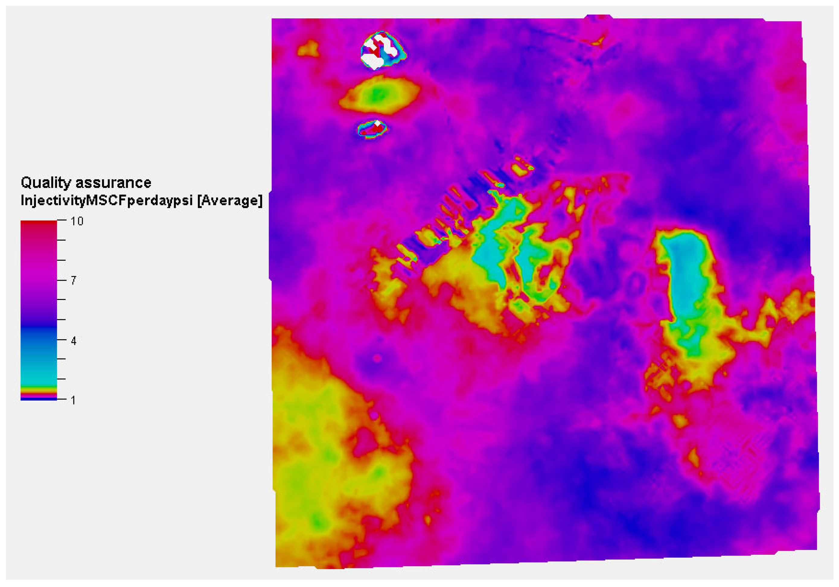
Following the validation of the Ridge regression model against field-derived correlations, the next step was to apply the model’s outputs spatially to evaluate how injectivity varies across the Entrada Formation. Figure 26 presents the averaged CO2 injectivity map, integrating results from all five simulated layers to reveal the formation’s overall injection potential within the San Juan Basin considering every gridblock as a potential well location.
The composite map highlights zones of persistent injectivity and serves as a guide for identifying optimal well placement targets. The central region extending toward the southwest emerges as the most favorable injection corridor. Injectivity values within this fairway typically range from 2 to 8 MSCF/day-psi, with localized peaks reaching approximately 10 MSCF/day-psi. This area not only records the highest injectivity magnitudes but also maintains strong lateral continuity across multiple layers, confirming its role as the primary zone for reliable and sustained CO2 injection. A secondary favorable domain appears toward the east and southeast, where injectivity averages within a similar range but across a smaller footprint. Although less extensive than the central–southwest fairway, this zone exhibits good connectivity and offers additional capacity for secondary injectors or future expansion, particularly for pressure management or distributed-rate injection strategies. In contrast, the north, towards the northwestern region coincides with the hogback monocline, a structurally complex area characterized by steeply rising and dipping beds. These structural conditions make it unsuitable for well-siting.
The observed injectivity trends are closely linked to geological factors such as the depositional architecture of the Entrada Formation. Zones of higher injectivity align with laterally continuous sand and coarse sand facies, where increased effective permeability thickness promotes efficient fluid inflow and pressure dissipation during injection. Across most of the modeled area, the structural surface is relatively gentle. However, structural influence becomes pronounced in the Hogback region, where steeply dipping strata disrupt reservoir continuity and pressure communication, making the area unsuitable for well placement. The anisotropy is generally low in magnitude and largely spatially uniform, averaging about 0.1. While it is not a dominant factor in this formation (as confirmed by sensitivity analysis), anisotropy provides a secondary influence in terms of lateral pressure propagation.
Overall, the averaged injectivity map reveals a coherent spatial pattern: a central–southwestern high-injectivity fairway supported by a smaller southeastern zone, both surrounded by lower-permeability margins associated with stratigraphic heterogeneity. This distribution underscores the Entrada Formation’s heterogeneous but well-organized flow system and provides a strong basis for strategic injector placement and long-term CO2 storage design.

4. Conclusions

This study developed an integrated framework combining reservoir simulation, sensitivity analysis, and machine learning proxy modeling to evaluate CO2 injectivity in the Entrada Sandstone of the San Juan Basin. The results demonstrate that this hybrid approach effectively captures both the physical and data-driven aspects of CO2 flow behavior in heterogeneous saline formations.
The calibrated reservoir model reproduced field behavior with a global history-match error of about 9.6%, confirming that the Entrada Formation’s pressure-rate dynamics are well represented. Forecast simulations showed stable injection behavior over a 30-year period, indicating that the formation can accommodate long-term CO2 storage without exceeding operational pressure limits. Sensitivity analysis revealed that permeability thickness ( k h ) and fractional flow slope (df/ds) are the dominant controls on injectivity, followed by anisotropy and heterogeneity (VDP). Geological factors clearly outweighed operational ones, emphasizing that injectivity performance is primarily a function of reservoir architecture and its flow properties.
Among the seven predictive models tested, Ridge regression achieved the best balance between accuracy, stability, and interpretability, with a blind R2 of 0.93. Unlike the ensemble models, Ridge provided transparent relationships between the input parameters and CO2 injectivity, showing that permeability anisotropy and k h strongly enhance injectivity, while higher heterogeneity and steeper fractional flow slopes are inversely related. Validation against the Mishra et al. [39] field-derived correlation confirmed the Ridge model’s physical realism. Its predictions aligned closely with the global J - k h envelope, clustering near the upper bound and indicating that the Entrada Formation behaves as a high-quality, laterally continuous reservoir.
Spatial application of the Ridge model revealed a central-to-southwestern high-injectivity fairway (2–8 MSCF/day-psi, locally up to 10 MSCF/day-psi) supported by a smaller southeastern zone as a secondary zone for injection. The northwestern region, associated with the hogback monocline, is structurally unsuitable for well placement but may enhance containment.
Collectively, these findings indicate that the Entrada Sandstone exhibits favorable injectivity characteristics and structural integrity for long-term CO2 storage. The Ridge regression model provides a physically interpretable, data-driven tool for predicting injectivity trends and guiding well placement decisions. Although this study focuses on the Entrada Sandstone of the San Juan Basin, it also contributes the modeling framework in addition to the basin-specific prediction. This workflow can be applied to other basins by redefining the model properties and operational conditions and retraining the proxy accordingly, particularly when model properties fall outside the ranges considered in this study. Application to non-sandstone reservoirs, such as carbonates or basalts, is feasible within the same framework, provided that the dominant injectivity controls are represented in the simulation model. Likewise, extension to more heterogeneous or fractured systems would require appropriate fracture representation to ensure that the governing flow behavior is captured before proxy training. Within these considerations, this integrated workflow offers a practical framework for future site screening, optimization, and risk assessment in carbon storage projects.

Author Contributions

Conceptualization, D.C.E. and W.A.; methodology, D.C.E., W.A., N.S. and D.B.; software, D.C.E. and N.S.; validation, D.C.E., W.A. and N.S.; formal analysis, D.C.E.; investigation, D.C.E. and N.S.; resources, W.A.; data curation, D.C.E.; writing—original draft preparation, D.C.E.; writing—review and editing, D.C.E., W.A., N.S. and D.B.; visualization, D.C.E.; supervision, W.A. and N.S.; project administration, W.A.; funding acquisition, W.A. All authors have read and agreed to the published version of the manuscript.

Funding

This research is funded by the U.S. Department of Energy’s National Energy Technology Laboratory under awards DE-FE0031890 and DE-FE0032363.

Data Availability Statement

The original contributions presented in this study are included in the article. Further inquiries can be directed to the corresponding author.

Conflicts of Interest

The authors declare no conflicts of interest.

Abbreviations

The following abbreviations are used in this manuscript:
IBDPIllinois Basin—Decatur Project
SECARBSoutheast Regional Carbon Sequestration Partnership
MRCSPMidwestern Regional Carbon Sequestration Partnership
AEPAmerican Electric Power
MLMachine Learning
SVRSupport Vector Regression
MSEMean Squared Error
MAEMean Absolute Error
BHPBottomhole Pressure
UDQUser-Defined Quantity
WGIRWell Gas Injection Rate
WBHPWell Bottomhole Pressure
FPRPField Average Pressure
LHSLatin Hypercube Sampling

References

  1. Li, Y. Dynamic Modelling and Monitoring of Geological Carbon Sequestration Assets. Ph.D. Thesis, Stanford University, Stanford, CA, USA, 2024. [Google Scholar]
  2. Essel, D.C.; Ampomah, W.; Sibaweihi, N.; Bui, D. Multi-Parameter Assessment of CO2 Injectivity for Optimal Well Siting in Geological Carbon Storage. In Proceedings of the SPE/AAPG/SEG Carbon Capture, Utilization, and Storage Conference and Exhibition, Houston, TX, USA, 23–25 April 2025. [Google Scholar]
  3. Machado, M.V.B.; Delshad, M.; Sepehrnoori, K. Injectivity assessment for CCS field-scale projects with considerations of salt deposition, mineral dissolution, fines migration, hydrate formation, and non-Darcy flow. Fuel 2023, 353, 129148. [Google Scholar] [CrossRef]
  4. Li, B.; Benson, S.M. Influence of small-scale heterogeneity on upward CO2 plume migration in storage aquifers. Adv. Water Resour. 2015, 83, 389–404. [Google Scholar] [CrossRef]
  5. Cui, G.; Wang, Y.; Rui, Z.; Chen, B.; Ren, S.; Zhang, L. Assessing the combined influence of fluid-rock interactions on reservoir properties and injectivity during CO2 storage in saline aquifers. Energy 2018, 155, 281–296. [Google Scholar] [CrossRef]
  6. Torsæter, M.; Cerasi, P. Geological and geomechanical factors impacting loss of near-well permeability during CO2 injection. Int. J. Greenh. Gas Control 2018, 76, 193–199. [Google Scholar] [CrossRef]
  7. Alamara, H.; Blondeau, C.; Thibeau, S.; Bogdanov, I. Vertical equilibrium simulation for industrial-scale CO2 storage in heterogeneous aquifers. Sci. Rep. 2025, 15, 17115. [Google Scholar] [CrossRef] [PubMed]
  8. Zeigler, B.P.; Moon, Y.; Kim, D.; Ball, G. The DEVS environment for high-performance modeling and simulation. IEEE Comput. Sci. Eng. 1997, 4, 61–71. [Google Scholar] [CrossRef]
  9. Lin, K.; Wei, N.; Zhang, Y.; Ali, M.; Chen, Q.; Wang, W.; Song, Z.; Yin, Y.; Vo Thanh, H. Advances in machine-learning-driven CO2 geological storage: A comprehensive review and outlook. Energy Fuels 2025, 39, 13315–13343. [Google Scholar] [CrossRef]
  10. Isah, A.; Tariq, Z.; Mustafa, A.; Mahmoud, M.; Okoroafor, E.R. A review of data-driven machine learning applications in reservoir petrophysics. Arab. J. Sci. Eng. 2025, 50, 20343–20377. [Google Scholar] [CrossRef]
  11. Hassija, V.; Chamola, V.; Mahapatra, A.; Singal, A.; Goel, D.; Huang, K.; Scardapane, S.; Spinelli, I.; Mahmud, M.; Hussain, A. Interpreting black-box models: A review on explainable artificial intelligence. Cogn. Comput. 2024, 16, 45–74. [Google Scholar] [CrossRef]
  12. Sahith, J.K.; Lal, B. Leveraging machine learning and artificial intelligence for enhanced carbon capture and storage (CCS). In Gas Hydrate in Carbon Capture, Transportation and Storage, 1st ed.; CRC Press: Boca Raton, FL, USA, 2024; pp. 159–196. [Google Scholar]
  13. Jun, C.; Kim, M.; Shin, H. Optimization of well placement and operating conditions for various well patterns in CO2 sequestration in the Pohang Basin, Korea. Int. J. Greenh. Gas Control 2019, 90, 102810. [Google Scholar] [CrossRef]
  14. Nordbotten, J.M.; Celia, M.A.; Bachu, S. Injection and storage of CO2 in deep saline aquifers: Analytical solution for CO2 plume evolution during injection. Transp. Porous Media 2005, 58, 339–360. [Google Scholar] [CrossRef]
  15. Whittle, T.; Park, P.; Coll, C. A semi-analytical model for the prediction of CO2 injectivity into saline aquifers or depleted hydrocarbon reservoirs. In Proceedings of the SPE Europec featured at EAGE Conference and Exhibition, Madrid, Spain, 6–9 June 2022. [Google Scholar]
  16. Mishra, S.; Ganesh, P.R.; Schuetter, J. Developing and validating simplified predictive models for CO2 geologic sequestration. Energy Procedia 2017, 114, 3456–3464. [Google Scholar] [CrossRef]
  17. Valluri, M.; Mishra, S.; Ganesh, P.R. Injectivity index: A powerful tool for characterizing CO2 storage reservoirs—A technical note. Greenh. Gases Sci. Technol. 2021, 11, 251–265. [Google Scholar] [CrossRef]
  18. Peng, L.; Han, G.; Chen, Z.; Pagou, A.L.; Zhu, L.; Abdoulaye, A.M. Dynamically coupled reservoir and wellbore simulation research in two-phase flow systems: A critical review. Processes 2022, 10, 1778. [Google Scholar] [CrossRef]
  19. McClure, M.W.; Horne, R.N. Investigation of injection-induced seismicity using a coupled fluid flow and rate/state friction model. Geophysics 2011, 76, WC181–WC198. [Google Scholar] [CrossRef]
  20. SLB. ECLIPSE Reservoir Simulation Reference Manual; Schlumberger Limited: Houston, TX, USA, 2024. [Google Scholar]
  21. Debossam, J.G.S.; de Freitas, M.M.; de Souza, G.; Amaral Souto, H.P.; Pires, A.P. Numerical Simulation of Non-Darcy Flow in Naturally Fractured Tight Gas Reservoirs for Enhanced Gas Recovery. Gases 2024, 4, 253–272. [Google Scholar] [CrossRef]
  22. Fu, Y.; Yuan, G.; Xia, Y.; Wang, M.; Zhang, Y.; Yang, X.; Wang, Z.; Cheng, Y. Research on improving injection and production gas capacity based on integrated reservoir-well coupling model for gas storage. Fuel 2025, 393, 135018. [Google Scholar] [CrossRef]
  23. Batzle, M.; Wang, Z. Seismic properties of pore fluids. Geophysics 1992, 57, 1396–1408. [Google Scholar] [CrossRef]
  24. Müller, N. Supercritical CO2-brine relative permeability experiments in reservoir rocks—Literature review and recommendations. Transp. Porous Media 2011, 87, 367–383. [Google Scholar] [CrossRef]
  25. Newman, G.H. Pore-volume compressibility of consolidated, friable, and unconsolidated reservoir rocks under hydrostatic loading. J. Pet. Technol. 1973, 25, 129–134. [Google Scholar] [CrossRef]
  26. Rajabi, M.M.; Ataie-Ashtiani, B.; Janssen, H. Efficiency enhancement of optimized Latin hypercube sampling strategies: Application to Monte Carlo uncertainty analysis and meta-modeling. Adv. Water Resour. 2015, 76, 127–139. [Google Scholar] [CrossRef]
  27. Zhou, X.; Al-Otaibi, F.; Kokal, S. Relative permeability characteristics and wetting behavior of supercritical CO2 displacing water and remaining oil for carbonate rocks at reservoir conditions. Energy Fuels 2019, 33, 5464–5475. [Google Scholar] [CrossRef]
  28. Dria, D.E.; Pope, G.A.; Sepehrnoori, K. Three-phase gas/oil/brine relative permeabilities measured under CO2 flooding conditions. SPE Reserv. Eng. 1993, 8, 143–150. [Google Scholar] [CrossRef]
  29. Mishra, S.; Ganesh, P.R. A screening model for predicting injection well pressure buildup and plume extent in CO2 geologic storage projects. Int. J. Greenh. Gas Control 2021, 106, 103261. [Google Scholar] [CrossRef]
  30. Luo, Z. Modeling Injection Induced Fractures and Their Impact in CO2 Geological Storage. Ph.D. Thesis, The University of Texas at Austin, Austin, TX, USA, 2013. [Google Scholar]
  31. Clavaud, J.B.; Maineult, A.; Zamora, M.; Rasolofosaon, P.; Schlitter, C. Permeability anisotropy and its relations with porous medium structure. J. Geophys. Res. Solid Earth 2008, 113, B01202. [Google Scholar] [CrossRef]
  32. Ganesh, P.R.; Mishra, S. Reduced physics modeling of CO2 injectivity. Energy Procedia 2014, 63, 3116–3125. [Google Scholar] [CrossRef]
  33. Russell, C.J.; Dean, M.A. To log or not to log: Bootstrap as an alternative to the parametric estimation of moderation effects in the presence of skewed dependent variables. Organ. Res. Methods 2000, 3, 166–185. [Google Scholar] [CrossRef]
  34. Maertens, K.; Baerdemaeker, J.D.; Babuška, R. Genetic polynomial regression as input selection algorithm for non-linear identification. Soft Comput. 2006, 10, 785–795. [Google Scholar] [CrossRef]
  35. Ahsan, M.M.; Mahmud, M.P.; Saha, P.K.; Gupta, K.D.; Siddique, Z. Effect of data scaling methods on machine learning algorithms and model performance. Technologies 2021, 9, 52. [Google Scholar] [CrossRef]
  36. Singh, V.; Pencina, M.; Einstein, A.J.; Liang, J.X.; Berman, D.S.; Slomka, P. Impact of train/test sample regimen on performance estimate stability of machine learning in cardiovascular imaging. Sci. Rep. 2021, 11, 14490. [Google Scholar] [CrossRef]
  37. Alemerien, K.; Alsarayreh, S.; Altarawneh, E. Diagnosing Cardiovascular Diseases using Optimized Machine Learning Algorithms with GridSearchCV. J. Appl. Data Sci. 2024, 5, 1539–1552. [Google Scholar] [CrossRef]
  38. Lin, S.; Zheng, H.; Han, B.; Li, Y.; Han, C.; Li, W. Comparative performance of eight ensemble learning approaches for the development of models of slope stability prediction. Acta Geotech. 2022, 17, 1477–1502. [Google Scholar] [CrossRef]
  39. Mishra, S.; Ganesh, P.R.; Valluri, M.; Jenkins, C. Practical Approaches for Estimating CO2 Injectivity Index in Saline Aquifers and Applications in De-Risking CCS Projects. In Proceedings of the 17th Greenhouse Gas Control Technologies Conference (GHGT-17), Calgary, AB, Canada, 20–24 October 2024. [Google Scholar]
  40. Baker, R.O.; Chugh, S.; McBurney, C.; McKishnie, R. History Matching Standards: Quality Control and Risk Analysis for Simulation. In Proceedings of the PETSOC Canadian International Petroleum Conference, Calgary, AB, Canada, 13–15 June 2006. [Google Scholar]
  41. Rezk, M.G.; Ibrahim, A.F. Numerical investigation of CO2 plume migration and trapping mechanisms in the Sleipner field: Does the aquifer heterogeneity matter? Fuel 2025, 394, 135054. [Google Scholar] [CrossRef]
  42. Bera, A.; Satapathy, S.; Daneti, J. Perspectives of CO2 injection strategies for enhanced oil recovery and storage in Indian oilfields. Energy Fuels 2024, 38, 10613–10633. [Google Scholar] [CrossRef]
  43. Punase, A.D. Assessing the Effect of Reservoir Heterogeneity on CO2 Plume Migration Using Pressure Transient Analysis. Master’s Thesis, University of Texas at Austin, Austin, TX, USA, 2012. [Google Scholar]
  44. Gupta, N.; Kelley, M.; Place, M.; Cumming, L.; Mawalkar, S.; Srikanta, M.; Pardini, R. Lessons learned from CO2 injection, monitoring, and modeling across a diverse portfolio of depleted closed carbonate reef oil fields–the Midwest Regional Carbon Sequestration Partnership experience. Energy Procedia 2017, 114, 5540–5552. [Google Scholar] [CrossRef]
  45. Ott, H. CO2-Brine Primary Displacement in Saline Aquifers: Experiments, Simulations and Concepts. Postdoctoral Thesis, RWTH Aachen University, Aachen, Germany, 2015. [Google Scholar]
  46. Odi, U.; Gupta, A. Fractional Flow Analysis of Displacement in a CO2 Enhanced Gas Recovery Process for Carbonate Reservoirs. In Proceedings of the International Conference on Offshore Mechanics and Arctic Engineering (OMAE), Rio de Janeiro, Brazil, 1–6 July 2012. [Google Scholar]
  47. Gasda, S.E.; Celia, M.A.; Nordbotten, J.M. Upslope plume migration and implications for geological CO2 sequestration in deep, saline aquifers. IES J. Part A Civ. Struct. Eng. 2008, 1, 2–16. [Google Scholar] [CrossRef]
  48. Tukey, J.W. Exploratory Data Analysis; Addison-Wesley: Reading, MA, USA, 1977. [Google Scholar]
  49. Chinhamu, K.; Chifurira, R. Evaluating South Africa’s market risk using asymmetric power auto-regressive conditional heteroscedastic model under heavy-tailed distributions. J. Econ. Financ. Sci. 2019, 12, 1–11. [Google Scholar]
  50. Maurya, S.K.; Yadav, A.S.; Singh, S.K.; Singh, U. A new flexible logarithmic transform heavy-tailed distribution and its applications. J. Stat. Manag. Syst. 2021, 24, 917–950. [Google Scholar] [CrossRef]
  51. Choi, G.; Buckley, J.P.; Kuiper, J.R.; Keil, A.P. Log-transformation of independent variables: Must we? Epidemiology 2022, 33, 843–853. [Google Scholar] [CrossRef]
  52. Enginar, O. Deep Ensembles Approach for Energy Forecasting. Ph.D. Thesis, Middle East Technical University, Ankara, Turkey, 2023. [Google Scholar]
  53. Hastie, T.; Tibshirani, R.; Friedman, J. The Elements of Statistical Learning, 2nd ed.; Springer: New York, NY, USA, 2009. [Google Scholar]
  54. Xia, L.; Nan, B.; Li, Y. A Revisit to De-biased Lasso for Generalized Linear Models. arXiv 2020, arXiv:2006.12778. [Google Scholar] [CrossRef]
  55. Zhang, Z.; Lai, Z.; Xu, Y.; Shao, L.; Wu, J.; Xie, G.S. Discriminative elastic-net regularized linear regression. IEEE Trans. Image Process. 2017, 26, 1466–1481. [Google Scholar] [CrossRef]
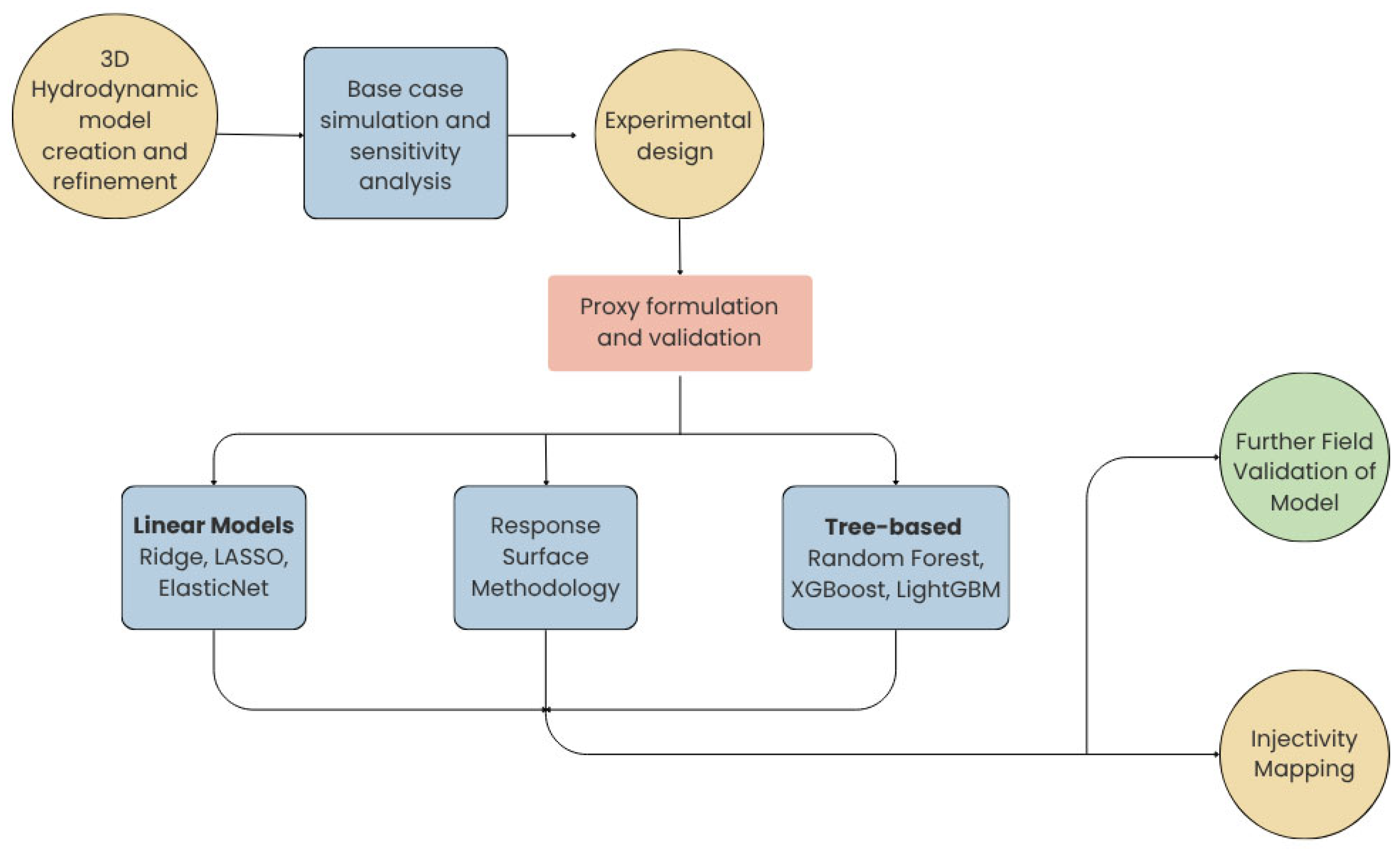
Figure 1. Workflow for CO2 injectivity prediction, from static model to final model validations and mapping.
Energies 19 00764 g001
Figure 2. The 3D geological model showing the two regions: the deactivated shallow hogback region and the central basin region where injection takes place (developed using Petrel and executed using ECLIPSE 2024.1 reservoir simulation software).
Energies 19 00764 g002
Figure 3. Field-derived correlation between CO2 injectivity index ( J ) and permeability-thickness ( k h ) product modified from Mishra et al. [39].
Energies 19 00764 g003
Figure 4. Final history matching results for water injection rate: (a) history-matched and observed injection rates for wells 1–3; (b) history-matched and observed injection rates for wells 4–6.
Energies 19 00764 g004
Figure 5. Final history matching results for bottomhole pressure: (a) history-matched and observed pressures for wells 1–3; (b) history-matched and observed pressures for wells 4–6.
Energies 19 00764 g005
Figure 6. CO2 plume distribution after 30 years of injection.
Energies 19 00764 g006
Figure 7. Pressure response following CO2 injection: (a) pressure distribution before injection; (b) pressure distribution after 30 years of injection; (c) change in pressure following CO2 injection.
Energies 19 00764 g007
Figure 8. Simulated trends in bottomhole pressure, gas injection rate, injectivity index, and cumulative CO2 injected.
Energies 19 00764 g008
Figure 9. Sensitivity analysis plot ranking the relative impact of parameters affecting CO2 injectivity, where parameters with longer bars exert a stronger influence on injectivity.
Energies 19 00764 g009
Figure 10. Distribution plot for X1 (VDP): (a) histogram with Kernel Density Estimate (KDE); (b) Q–Q plot; (c) boxplot; (d) Empirical Cumulative Distribution Function (ECDF).
Energies 19 00764 g010
Figure 11. Distribution plot for X2 (permeability anisotropy): (a) histogram with Kernel Density Estimate (KDE); (b) Q–Q plot; (c) boxplot; (d) Empirical Cumulative Distribution Function (ECDF).
Energies 19 00764 g011
Figure 12. Distribution plot for X3 (df/ds): (a) histogram with Kernel Density Estimate (KDE); (b) Q–Q plot; (c) boxplot; (d) Empirical Cumulative Distribution Function (ECDF).
Energies 19 00764 g012
Figure 13. Distribution plot for X4 ( k h ) before transformation: (a) histogram with Kernel Density Estimate (KDE); (b) Q–Q plot; (c) boxplot; (d) Empirical Cumulative Distribution Function (ECDF).
Energies 19 00764 g013
Figure 14. Distribution plot for X4 ( k h ) after logarithmic transformation: (a) histogram with Kernel Density Estimate (KDE); (b) Q–Q plot; (c) boxplot; (d) Empirical Cumulative Distribution Function (ECDF).
Energies 19 00764 g014
Figure 15. Distribution plot for Y (CO2 injectivity) before transformation: (a) histogram with Kernel Density Estimate (KDE); (b) Q–Q plot; (c) boxplot; (d) Empirical Cumulative Distribution Function (ECDF).
Energies 19 00764 g015
Figure 16. Distribution plot for Y (CO2 injectivity) after logarithmic transformation: (a) histogram with Kernel Density Estimate (KDE); (b) Q–Q plot; (c) boxplot; (d) Empirical Cumulative Distribution Function (ECDF).
Energies 19 00764 g016
Figure 17. Pairplot showing relationships in the transformed injectivity dataset.
Energies 19 00764 g017
Figure 18. Performance evaluation of the Response Surface model on the blind dataset: (a) parity plot comparing predicted and actual CO2 injectivity values, where the dashed line represents perfect agreement and deviations indicate prediction error; (b) residual distribution for the blind dataset, illustrating the magnitude and spread of prediction errors.
Energies 19 00764 g018
Figure 19. Performance evaluation of the LightGBM model on the blind dataset: (a) parity plot comparing predicted and actual CO2 injectivity values, where the dashed line represents perfect agreement and deviations indicate prediction error; (b) residual distribution for the blind dataset, illustrating the magnitude and spread of prediction errors.
Energies 19 00764 g019
Figure 20. Performance evaluation of the XGBoost model on the blind dataset: (a) parity plot comparing predicted and actual CO2 injectivity values, where the dashed line represents perfect agreement and deviations indicate prediction error; (b) residual distribution for the blind dataset, illustrating the magnitude and spread of prediction errors.
Energies 19 00764 g020
Figure 21. Performance evaluation of the ElasticNet model on the blind dataset: (a) parity plot comparing predicted and actual CO2 injectivity values, where the dashed line represents perfect agreement and deviations indicate prediction error; (b) residual distribution for the blind dataset, illustrating the magnitude and spread of prediction errors.
Energies 19 00764 g021
Figure 22. Performance evaluation of the Lasso model on the blind dataset: (a) parity plot comparing predicted and actual CO2 injectivity values, where the dashed line represents perfect agreement and deviations indicate prediction error; (b) residual distribution for the blind dataset, illustrating the magnitude and spread of prediction errors.
Energies 19 00764 g022
Figure 23. Performance evaluation of the Random Forest model on the blind dataset: (a) parity plot comparing predicted and actual CO2 injectivity values, where the dashed line represents perfect agreement and deviations indicate prediction error; (b) residual distribution for the blind dataset, illustrating the magnitude and spread of prediction errors.
Energies 19 00764 g023
Figure 24. Performance evaluation of the Ridge model on the blind dataset: (a) parity plot comparing predicted and actual CO2 injectivity values, where the dashed line represents perfect agreement and deviations indicate prediction error; (b) residual distribution for the blind dataset, illustrating the magnitude and spread of prediction errors.
Energies 19 00764 g024
Figure 25. Comparison of Ridge-predicted injectivity values with the empirical correlation range modified from Mishra et al. [39].
Energies 19 00764 g025
Figure 26. Average CO2 injectivity map integrating all five Entrada Formation layers in the San Juan Basin.
Energies 19 00764 g026
Table 1. Model performance (R2) evaluation under varying data split configurations.
Model\Test Size 0.100.200.250.30.4
Random Forest0.9910.9890.9860.9850.977
XGBoost0.9900.9910.9910.9890.980
Ridge0.9840.9840.9790.9800.981
ElasticNet0.9790.9820.9800.9820.978
LightGBM0.9770.9690.9700.9640.911
Lasso0.9720.9750.9730.9780.972
Response Surface (SVR)0.8170.203−0.270−0.098−0.794
Table 2. Average metrics across all models after train–test ratio sensitivity analysis.
Test SizeMean R2Mean MAEMean MSE
0.100.9616.781490.22
0.200.8716.574576.11
0.25−0.0322.79142,950.84
0.30−0.0119.2751,445.84
0.40−0.1128.61405,888.61
Table 3. Model performance summary (train/test dataset).
Model Train MSETrain MAETrain R2 Test MSETest MAETrain R2
Random Forest40.8552.6980.998164.7377.5620.994
Ridge271.3328.8690.988175.6027.3470.994
XGBoost54.7403.5230.997187.5135.4250.993
ElasticNet379.96610.0070.983851.04013.6080.971
Response Surface1209.35518.3030.945872.49918.7350.970
LightGBM252.8775.5790.9881010.74115.6760.965
Lasso474.32910.7380.9781211.44716.0680.958
Table 4. Comparative performance of all models on the blind dataset.
ModelBlind MSEBlind MAEBlind R2
Random Forest344.3811.170.93
Ridge410.5411.030.93
Lasso460.3110.970.92
ElasticNet554.9012.030.90
XGBoost640.7515.430.88
LightGBM1901.1223.820.66
Response Surface95,860.7278.35−0.16
Disclaimer/Publisher’s Note: The statements, opinions and data contained in all publications are solely those of the individual author(s) and contributor(s) and not of MDPI and/or the editor(s). MDPI and/or the editor(s) disclaim responsibility for any injury to people or property resulting from any ideas, methods, instructions or products referred to in the content.