Optimized Elbow Design for Hydrogen Pipeline Using Multi-Objective Genetic Algorithm

Abstract

In 90° elbows, abrupt turning induces strong secondary flow, separation, and turbulence, increasing pressure loss and degrading velocity uniformity. A hydrogen pipeline elbow is optimized by combining a nature-inspired cross-section with a guide vane, while tuning vane position/angle and geometric radii/offsets using a multi-objective genetic algorithm (MOGA). Three-dimensional CFD is performed for compressible gaseous hydrogen using the Peng–Robinson equation of state and the SST k–ω turbulence model. Design points are generated by Latin hypercube sampling, and response surface models based on non-parametric regression (NPR) and genetic aggregation (GA) guide the search. Relative to the reference elbow, the GA-based optimum improves velocity uniformity by 5.825% and reduces the total pressure-drop coefficient by 0.470%; the NPR-based optimum yields 4.021% and 0.229%, respectively. Flow-field analysis shows reduced separation area, axial vorticity, turbulent kinetic energy, and dissipation, indicating suppressed secondary flow and smoother turning. These gains translate to lower pumping power and enhanced energy efficiency, supporting cost-effective deployment of carbon-neutral hydrogen infrastructure.

1. Introduction

Unlike conventional fossil fuels, hydrogen is a clean, carbon-free energy source whose only by-product of combustion is water, making it a key energy source for realizing a sustainable and carbon-neutral future. As a result, research and investment in the development of infrastructure to efficiently transport and distribute hydrogen around the world is ongoing. Among hydrogen transport methods, pipeline transport systems are considered to be an efficient solution for long-distance transport. Pipeline-based transport systems have the advantages of high transport capacity, continuous supply, and relatively low operating costs [1]. However, hydrogen has distinct physical properties, including low molecular weight, low density, and high diffusivity, which pose technical challenges in pipeline transport. In elbow sections, hydrogen can exhibit flow characteristics that differ from those of conventional gases because pressure-induced density variation interacts with curvature-driven secondary flow, separation and reattachment, and turbulence production. For comparable transport requirements, hydrogen’s low density can lead to relatively higher bulk velocities, which increases dynamic pressure and amplifies losses associated with strong curvature, mixing, and dissipation. In addition, rapid pressure variation through an elbow can induce density changes, and consistent treatment of compressibility becomes increasingly important at elevated operating pressures where real-gas behaviour may need to be considered [2]. Consequently, elbows in hydrogen pipelines can experience intensified flow separation and enhanced energy dissipation, resulting in larger pressure drops and reduced transport efficiency.

To address these complex issues and increase transportation efficiency and economy, research is actively being conducted. Related studies have pointed out that the main cause of energy consumption in fluid transmission systems is the resistance of local components, and emphasized that geometry optimization, especially of elbows, is important to reduce the overall system resistance [3,4,5,6,7]. A previous study proposed a low-resistance local component geometry optimization method based on nature-inspired design and machine learning and verified the resistance reduction effect and mechanism of the optimized elbow, showing that 19% to 26% resistance reduction is achieved depending on the pipe diameter and Reynolds number [4]. Nature-inspired design aims to incorporate streamlined geometric features observed in nature to mitigate abrupt turning and energy dissipation. In elbow flows, such geometric features can promote smoother flow turning and reduce losses associated with curvature-induced mixing and separation. Here, guide vanes refer to passive flow-control elements installed inside elbows to align streamlines and weaken secondary-flow structures, thereby reducing separation-induced losses, suppressing turbulence generation, and improving velocity uniformity [8]. In the present work, the nature-inspired concept is realized through cross-sectional morphing in combination with guide-vane control. This study aims to find an optimized elbow geometry that reduces pressure drops, increases velocity uniformity, and reduces energy losses compared to conventional elbows by referring to these previous studies.

In this study, we optimized the elbow geometry using a genetic algorithm, which enables broad exploration of candidate designs in large and complex search spaces. In particular, when combined with computational fluid dynamics (CFD) simulation results for flow characterization, genetic algorithms perform well in complex pipe geometry optimization problems [3]. Yoshimura et al. [9] proposed a nonlinear-based approach for topology optimization using genetic algorithms, demonstrating an effective method for flow channel design. Zhang et al. [10] developed a multi-objective genetic algorithm (MOGA) based design method for flow performance optimization of dual-plane elbows, which succeeded in improving the flow uniformity coefficient and pressure drop coefficient simultaneously. However, most existing studies were conducted using incompressible fluids such as water or air as the working fluid, and there is a lack of elbow optimization studies that treat hydrogen using compressible and real-gas modeling. Therefore, this study focuses on optimizing a hydrogen elbow by performing CFD simulations with compressible gaseous hydrogen modeled using the Peng–Robinson equation of state and deriving the optimal elbow geometry using a genetic algorithm.

2. Theoretical Background

2.1. Velocity Uniformity

Velocity uniformity is used as a metric to evaluate the performance of elbows. Velocity uniformity refers to how evenly the flow of a fluid is distributed and is closely related to turbulence generation and pressure drop, especially in areas of high flow variation such as elbows [10]. Poor velocity uniformity can lead to increased pressure drop, vibration and noise generation, and poor heat transfer at certain locations [11]. Therefore, it is important to use the velocity uniformity index in piping design to evaluate and improve flow quality. Velocity uniformity can be defined as the difference between the velocity in each cell and the average velocity, expressed in absolute value, divided by the average velocity.

$$\mathrm{Uniformity} \mathrm{Index}=1-{\displaystyle \frac{{\int }_A\left|u-\overline{u}\right|dA}{{\int }_A\overline{u}dA}}$$

(1)

where u is the local velocity and $\overline{u}$ is the average velocity over the cross-sectional area.

2.2. Total Pressure Drop Coefficient

The total pressure drop coefficient is an important metric for evaluating the resistance inside a flow system and is often used to dimensionless express the pressure drop that occurs in common fluidic devices such as elbows and valves [12]. The total pressure drop coefficient is the total pressure drop divided by the dynamic pressure at the inlet, which is given by the following equation:

$$K={\displaystyle \frac{{\mathrm{p}}_{\mathrm{t},\mathrm{in}}-{\mathrm{p}}_{\mathrm{t},\mathrm{out}}}{\frac{1}{2}\mathsf{\rho }{U}^2}}$$

(2)

where ${\mathrm{p}}_{\mathrm{t}}$ is the total pressure, ${\mathrm{p}}_{\mathrm{i}\mathrm{n}}$ and ${\mathrm{p}}_{\mathrm{o}\mathrm{u}\mathrm{t}}$ are the total pressures at the elbow inlet and elbow outlet, respectively, ρ is the fluid density, and $U$ is the average velocity at the inlet.

The total pressure drop factor is typically used for incompressible flows and low-velocity compressible flows, where the velocity of the compressible flow is Mach number 0.3 or less.

2.3. Peng–Robinson Equation of States

An equation of state is an equation that describes the behavior of a gas in a compressible flow and is a mathematical expression of the pressure, volume, and temperature of a gas and is used to describe the thermodynamic state of a fluid. The simplest equation of state is the “ideal gas equation of state”. However, since real gases are affected by intermolecular attraction and volume, it is difficult to predict accurate properties using the ideal gas equation alone, so various equations of state for real gases have been developed to complement it [13]. Among them, the Peng–Robinson equation of state is a cubic form of the equation of state developed in 1976 and is shown as follows:

$$P={\displaystyle \frac{RT}{V-b}}-{\displaystyle \frac{a\left(T\right)}{V\left(V+b\right)+b\left(V-b\right)}}$$

(3)

where $V$ is the molar volume, $R$ is the ideal gas constant, $T$ is the absolute temperature, $\mathsf{\alpha }\left(T\right)$, and $a$ and $b$ are parameters that reflect the properties of each gas.

The Peng-Robinson equation of state is a more accurate equation of state for compressible flow conditions in high-pressure environments than the ideal gas equation of state because it considers intermolecular attraction distances [14,15]. These features make the Peng–Robinson equation of state useful for analyzing the flow properties of compressible fluids in high-pressure environments, such as hydrogen pipeline systems, and enable accurate thermodynamic modeling.

2.4. Energy Dissipation

Nature inspired is an approach to solving engineering problems that draws inspiration from the natural world and offers an effective alternative for reducing energy losses in fluid systems. Inspired by the meandering waterways of the Yellow River in China, Tian et al. [4] demonstrated that flow resistance can be reduced through geometries that mimic nature. Through experiments and simulations, they have shown that the fundamental cause of fluid flow resistance is energy dissipation, the process by which mechanical energy is converted into internal energy. Therefore, the less energy dissipation, the less fluid flow resistance; for a compressible flow, the energy equation could be written as follows:

$${\displaystyle \frac{\partial \left(\mathsf{\rho }E\right)}{\partial t}}+\nabla \cdot \left[\left(\mathsf{\rho }E+p\right)\overrightarrow{v}\right]=\nabla \cdot \left(k\nabla T\right)+\mathsf{\Phi }$$

(4)

where E is the total energy per unit mass, defined as the sum of internal energy € and kinetic energy. $\mathsf{\Phi }$ represents the energy dissipation term due to viscosity inside the fluid and is defined as:

$$\mathsf{\Phi }={\mathsf{\tau }}_{ij}{\displaystyle \frac{\partial u_i}{\partial x_j}}$$

(5)

where ${\mathsf{\tau }}_{ij}$ is the viscous stress tensor, expressed as:

$${\mathsf{\tau }}_{ij}=\mathsf{\mu }\left({\displaystyle \frac{\partial u_i}{\partial x_j}}+{\displaystyle \frac{\partial u_j}{\partial x_i}}\right)-{\displaystyle \frac{2}{3}}\mathsf{\mu }\left(\nabla \cdot \overrightarrow{v}\right){\mathsf{\delta }}_{ij}$$

(6)

where $\mathsf{\mu }$ is the dynamic viscosity coefficient and ${\mathsf{\delta }}_{ij}$ is the Kronecker delta function. $\nabla \cdot \overrightarrow{v}$ is the strain tensor, which is non-zero for compressible flow conditions.

3. Numerical Analysis

3.1. Pipeline Geometry

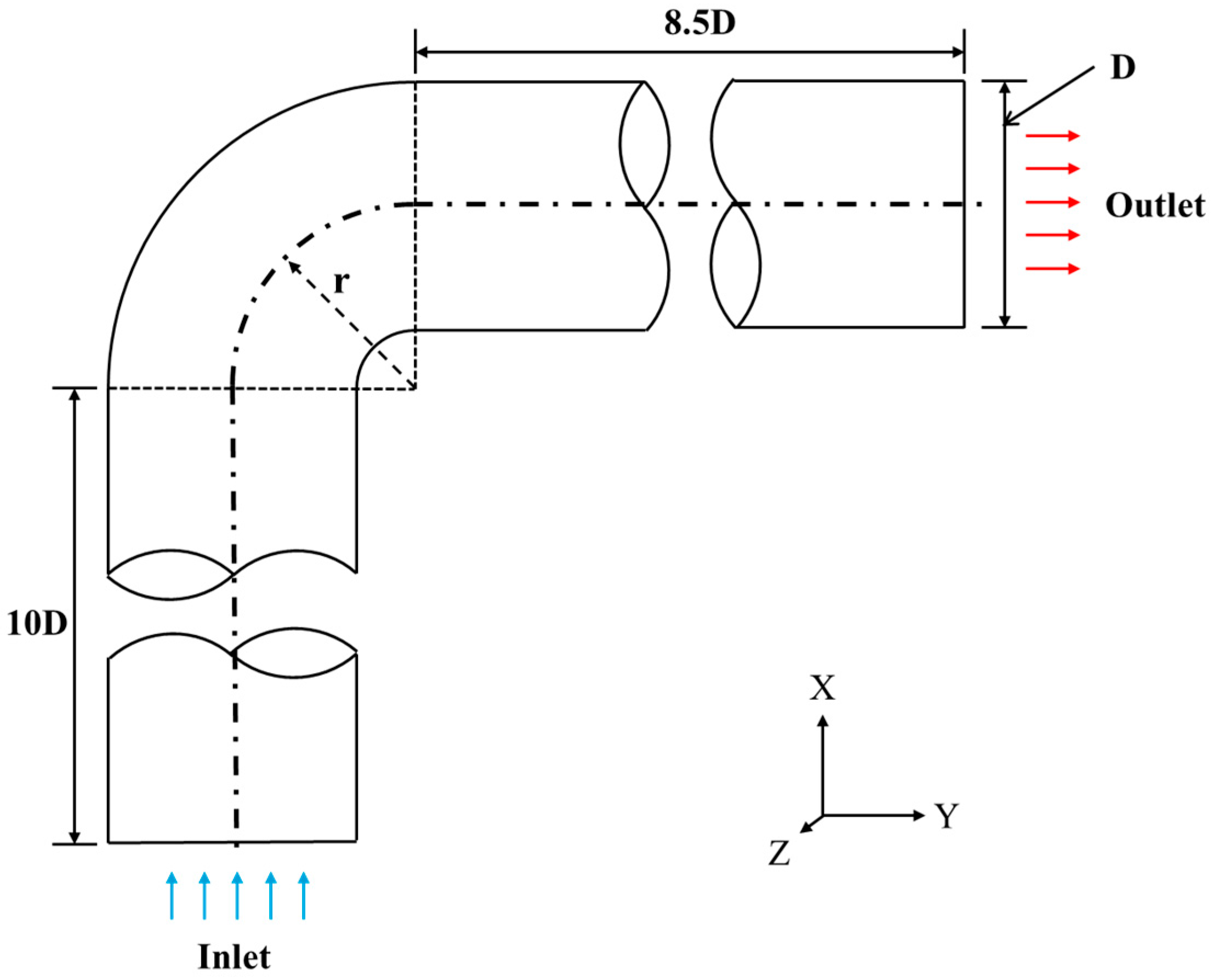
In this study, a circular cross-sectional pipe with a 90-degree bend angle is selected as a model. The diameter (D) of the pipe is 0.1 m, and the radius length (r/D) of the elbow is set to 1. The lengths of upstream and downstream are set to 10D and 8.5D, respectively, to allow the flow to develop fully, and the details are shown in Figure 1 and

Table 1. Geometrical parameters of the modeled pipeline elbow.

Variable	Value [m]
D	0.1
r	0.1
r/D	1

.

3.2. Governig Equations

In this study, the compressible three-dimensional Reynolds-averaged Navier–Stokes (RANS) equation is solved using the finite volume method, and numerical analysis is performed. In compressible flow, the law of conservation of mass is expressed by the continuity equation, which is an equation that preserves the relationship between the density change of the fluid and the inflow and outflow mass fluxes.

$${\displaystyle \frac{\partial \mathrm{ }\rho }{\partial \mathrm{ }t}}\mathrm{ }+\mathrm{ }\nabla \mathrm{ }\cdot \mathrm{ }\left(\rho \mathrm{ }\overrightarrow{v}\right)\mathrm{ }=\mathrm{ }0$$

(7)

where $\rho$ is the density of the fluid and $\overrightarrow{v}$ is the velocity vector.

The momentum equation is based on Newton’s second law and describes the change in momentum due to pressure, viscous and volumetric forces acting on fluid particles. The equation for conservation of momentum in a compressible flow can be represented as follows:

$${\displaystyle \frac{\partial \left(\rho \overrightarrow{v}\right)}{\partial t}}+\nabla \cdot \left(\rho \overrightarrow{v}\otimes \overrightarrow{v}\right)=-\nabla p+\nabla \cdot \overline{\overline{\tau }}+\rho \overrightarrow{g}$$

(8)

where p is the pressure, $\stackrel{̿}{\tau }$ is the viscous stress tensor, and $\overrightarrow{g}$ is the gravitational acceleration.

3.3. Turbulent Flow

The selection of an appropriate turbulence model is essential for accurate prediction of complex flow phenomena [3]. In this study, based on the results of these previous studies, we selected a turbulence model that can best reflect the characteristics of hydrogen flow. Studies such as [8,15,16] have shown that the velocity profiles obtained from numerical simulations using the shear stress transport (SST) $k-\mathsf{\omega }$ model are in good agreement with experimental results. Based on a comprehensive literature review, the SST $k-\mathsf{\omega }$ turbulence model was chosen for accurate prediction of secondary flow distribution and resistance losses in the near-wall boundary layer region for the current numerical solution. Menter [17] developed a two-equation SST $k-\mathsf{\omega }$ turbulence model incorporating the standard $k-\mathsf{\omega }$ model, where the standard $k-\mathsf{\omega }$ model was discovered by Wilcox et al. [18] for near-wall boundary layer flow and integrated with the standard $k-\mathsf{ϵ}$ model proposed by Jones and Launder [19] for free flow. By combining the two models, the SST $k-\mathsf{\omega }$ model effectively resolves the complexity of turbulent behavior both near walls and in the free flow region. The flow field is determined by solving the transport equations for the turbulent kinetic energy (k, ${\mathrm{m}}^2/{\mathrm{s}}^2$) and turbulent dissipation rate ($\mathsf{\omega }$, ${\mathrm{s}}^{-1}$) according to the SST $k-\mathsf{\omega }$ turbulence model.

$${\displaystyle \frac{\partial }{\partial x_i}}\left(\mathsf{\rho }k{u}_i\right)=P_k-{\mathsf{\beta }}^{*}\mathsf{\rho }k\mathsf{\omega }+{\displaystyle \frac{\partial }{\partial x_i}}\left[\mathsf{\mu }+{\mathsf{\sigma }}_k{\mathsf{\mu }}_t{\displaystyle \frac{\partial k}{\partial x_i}}\right]$$

(9)

$${\displaystyle \frac{\partial }{\partial x_i}}\left(\mathsf{\rho }\mathsf{\omega }{u}_i\right)=\mathsf{\alpha }{\displaystyle \frac{P_k}{{\mathsf{\mu }}_t}}-{\mathsf{\beta }}^{*}\mathsf{\rho }{\mathsf{\omega }}^2+{\displaystyle \frac{\partial }{\partial x_i}}\left[\mathsf{\mu }+{\mathsf{\sigma }}_{\mathsf{\omega }}{\mathsf{\mu }}_t{\displaystyle \frac{\partial \mathsf{\omega }}{\partial x_i}}\right]+2\left(1-F_1\right)\mathsf{\rho }{\mathsf{\sigma }}_{\mathsf{\omega }}^2{\displaystyle \frac{1}{\mathsf{\omega }}}{\displaystyle \frac{\partial k}{\partial x_i}}{\displaystyle \frac{\partial \mathsf{\omega }}{\partial x_i}}$$

(10)

where $P_k$ is the generating term, $\mathsf{\mu }$ and ${\mathsf{\mu }}_t$ represent the dynamic viscosity and turbulent viscosity coefficients, respectively, and $F_1$ is the definition of the mixing function. The model uses two key variables, the turbulent kinetic energy (k) and the specific dissipation rate (ω), to govern the turbulent transport equation, which allows it to accurately predict the properties of the flow field [20]. For a more comprehensive description of the SST $k-\mathsf{\omega }$ turbulence model, the reader can refer to the work of [21]. The coefficients $\mathsf{\beta }$, ${\mathsf{\beta }}^{*}$, $\mathsf{\alpha }$, ${\mathsf{\sigma }}_k$, and ${\mathsf{\sigma }}_{\omega }$ are defined based on the coefficients of the original $k-\mathsf{\omega }$ turbulence model and the converted $k-\mathsf{ϵ}$ model, which ensures consistency between the two approaches [22].

3.4. Boundary Conditions

The working fluid was selected as gaseous hydrogen with a temperature of 300 K. The Peng–Robinson equation of state was applied to accurately model the non-ideal behavior of hydrogen. The operating pressure was set to 2 MPa to reflect the high-pressure environment of the pipeline. The inlet condition was set to a Reynolds number of 17,600. The outlet condition was set to pressure outlet. A no-slip boundary condition was applied to the pipe wall to accurately reflect the effect of wall friction on the flow. These boundary conditions accurately reproduce the physical properties of the flow field and contribute to effectively capturing the complexity of high-pressure hydrogen flow in particular [23]. A steady-state, pressure-based solver was used, and the coupled algorithm was employed for the coupling between pressure and velocity. Furthermore, the residuals for the continuation equations, velocity, turbulent kinetic energy, and diffusion are defined with the convergence condition as ${10}^{-5}$.

3.5. Grid Dependency Test

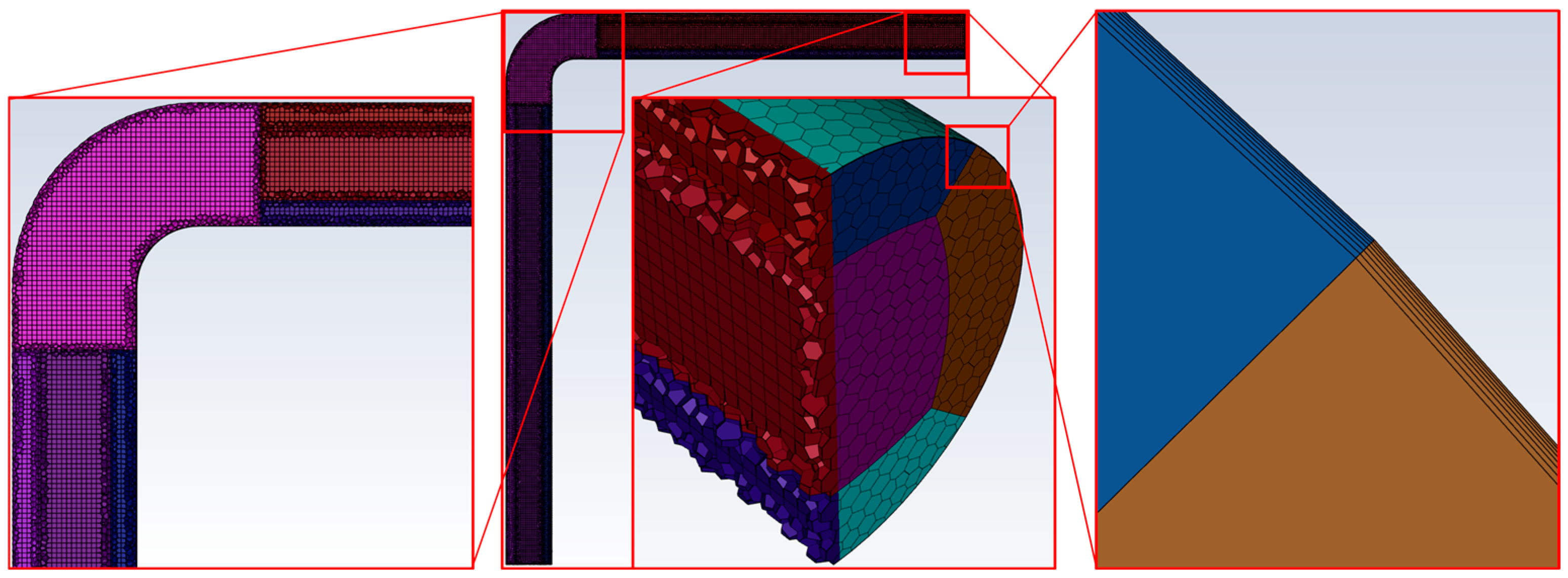
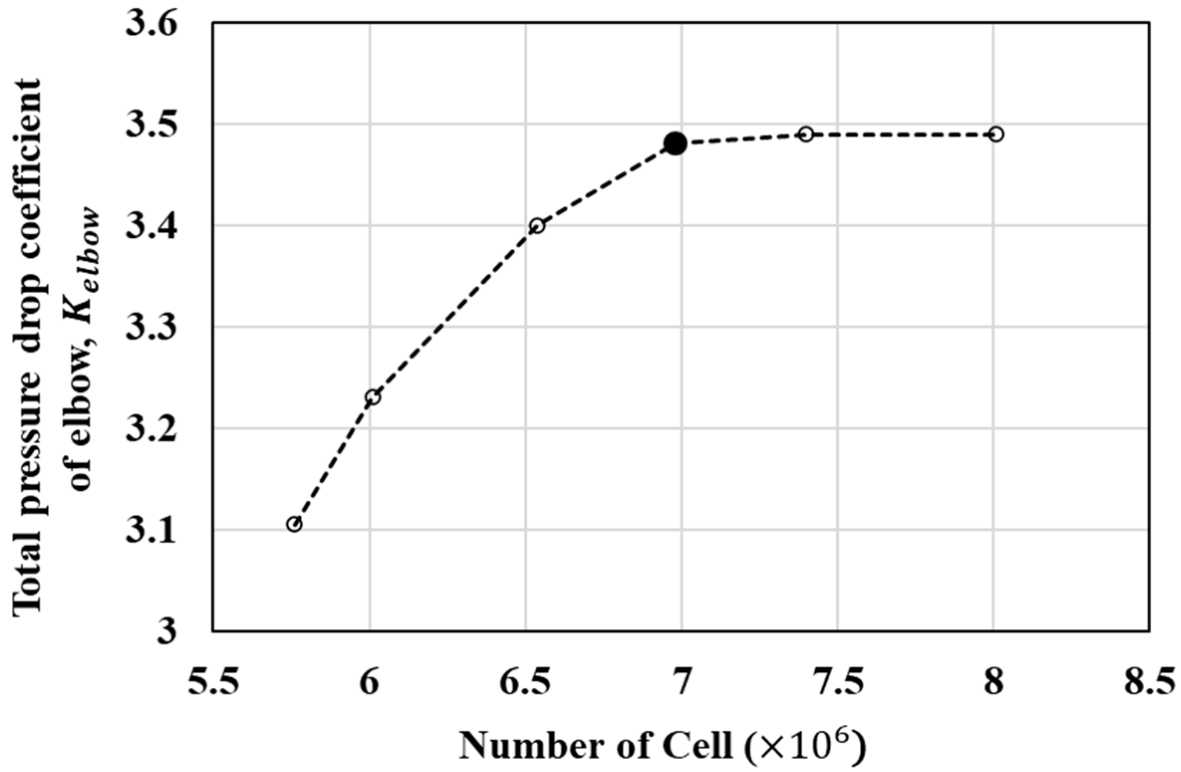
In this study, a grid was constructed to analyze the flow performance of the 90$°$ elbow and is shown in Figure 2. The pipe gird was partitioned into block-like sub-regions with arc-shaped boundaries to enable an O-grid–type poly-hexcore mesh, improving orthogonality and reducing skewness. The colours in Figure 2 are used to distinguish the divided mesh sections and have no physical meaning. For visibility, a coarse mesh was used as an example instead of the actual mesh employed. A denser grid was constructed to analyze the flow in the elbow region more accurately, and the dimensionless wall distance $y^{+}$ was kept below 1 to accurately capture the boundary layer flow. To determine the optimal number of grids to lower the computational cost and increase the efficiency of the analysis, a grid dependence test on the total pressure drop coefficient of elbow was performed. A total of six different grids were compared in the test, and the test results are shown in Figure 3 and

Table 2. Number of grids and pressure total drop coefficient of elbow.

$\mathbf{Cell} \mathbf{Number} (\times$106)	Total Pressure Drop Coefficient of Elbow, Kelbow
5.76	3.1056
6.01	3.2311
6.54	3.4001
6.98	3.4813
7.40	3.4901
8.01	3.4899

. The variation K_elbow converged to within 0.25% when the number of grids was more than $6.98\times {10}^6$, so these grids were finally selected for both accuracy and efficiency of calculation.

3.6. Validation

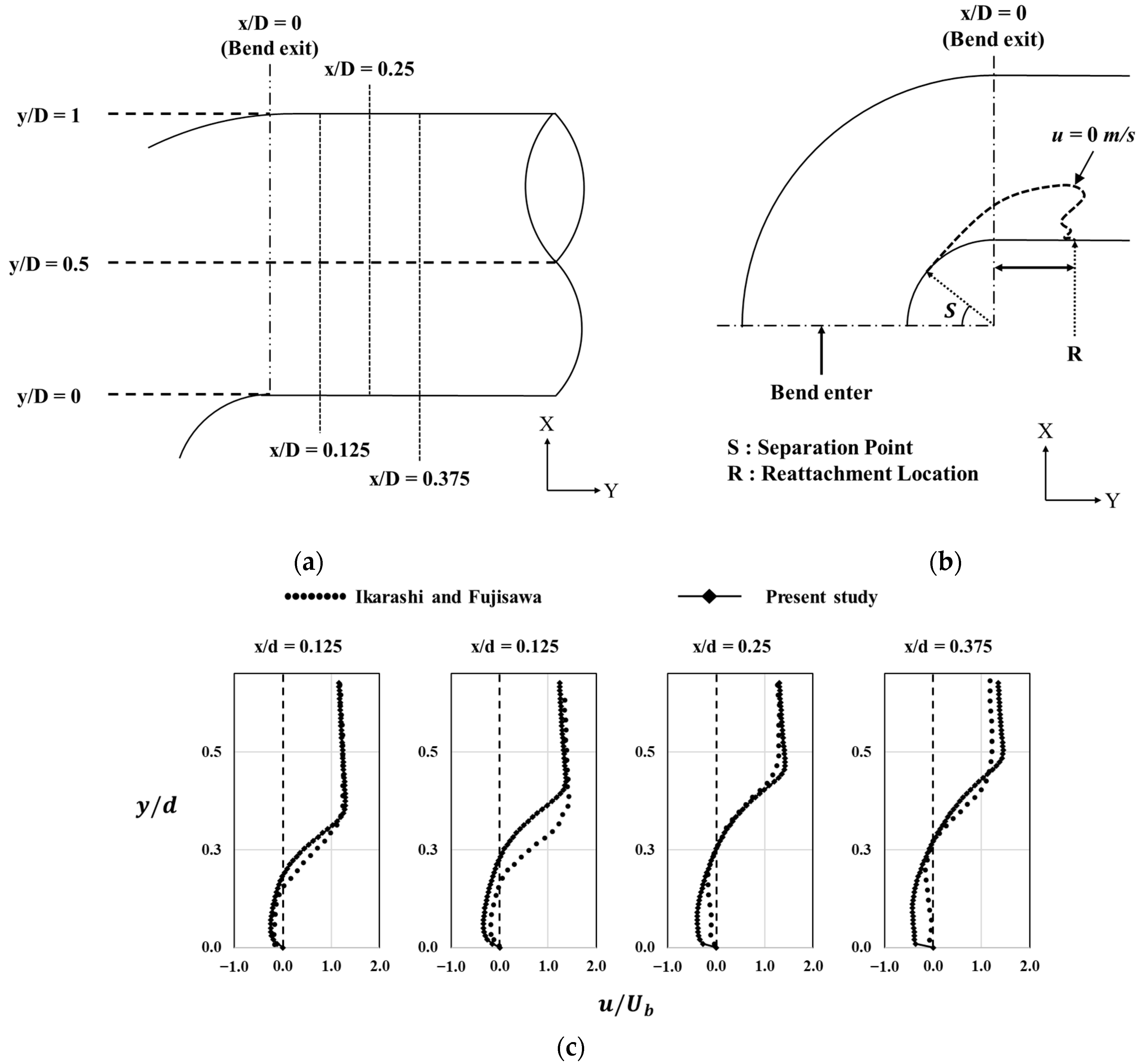
For validation, a baseline configuration without guide vanes (non-guide-vane case) was simulated using a 6.98 M mesh. The axial velocity profiles at the elbow exit were extracted along the radial direction (y/D) and compared with the experimental data reported by Ikarashi et al. at four downstream locations (x/D = 0, 0.125, 0.25, 0.375) (see Figure 4a,b) [24]. Overall, good agreement was obtained across all measurement locations, indicating that the present numerical setup captures the key flow features in the near-exit region.

In addition, the separation and reattachment locations were identified based on the sign change of the near-wall axial velocity along the inner wall (onset/termination of reverse flow) and compared with the literature values. Ikarashi et al. reported the separation point at alpha = 36.0 deg and the reattachment location at x/D = 0.50, whereas the present simulations predicted $\alpha =37.0°$ and x/D = 0.56, corresponding to relative errors of approximately 2.8% and 12%, respectively [24]. This quantitative consistency, together with the velocity-profile comparison shown in Figure 4c, supports that the adopted geometry, mesh resolution, and turbulence model can realistically reproduce the primary flow behavior in a $90°$ short elbow, including separation and reattachment and the near-exit velocity distribution.

Although water was used in the validation to allow a direct comparison with the available experiment, the subsequent analyses and optimization were performed for hydrogen under low-Mach-number conditions. In this regime, the dominant elbow-flow structures are primarily governed by geometric similarity (r/D) and Reynolds-number similarity. Therefore, the validated geometry/mesh strategy and turbulence model were consistently applied to the hydrogen cases.

Figure 4. Schematic of positions for validation: (a) Measurement position of axial velocity, (b) schematic of separation and reattachment positions, (c) validation of the axial velocity profile at the elbow exit based on the experimental results [24].

Figure 4. Schematic of positions for validation: (a) Measurement position of axial velocity, (b) schematic of separation and reattachment positions, (c) validation of the axial velocity profile at the elbow exit based on the experimental results [24].

4. Optimization

4.1. Numerical Simulation

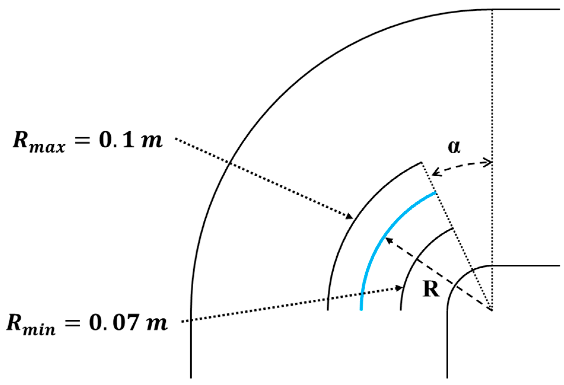
In this study, a design of experiments (DOE) framework was used to systematically relate the design variables to the objective functions and to generate a set of informative design points. The sampling and parameter study were conducted using ANSYS DesignXplorer (2024 R1), and the design points were generated via Latin hypercube sampling (LHS). LHS provides a space-filling distribution of samples across the design domain while minimizing redundancy among points, thereby supporting efficient exploration of the design space [25]. The geometrical design variables consisted of two variables related to the guide vane and three variables related to nature inspired to analyze their combined effects on flow characteristics. The design variables related to the guide vane are the position of the guide vane and the angle from the bend exit. The thickness of the guide vanes was fixed at 2 mm to reduce flow disturbance, and the vanes were rounded at the ends.

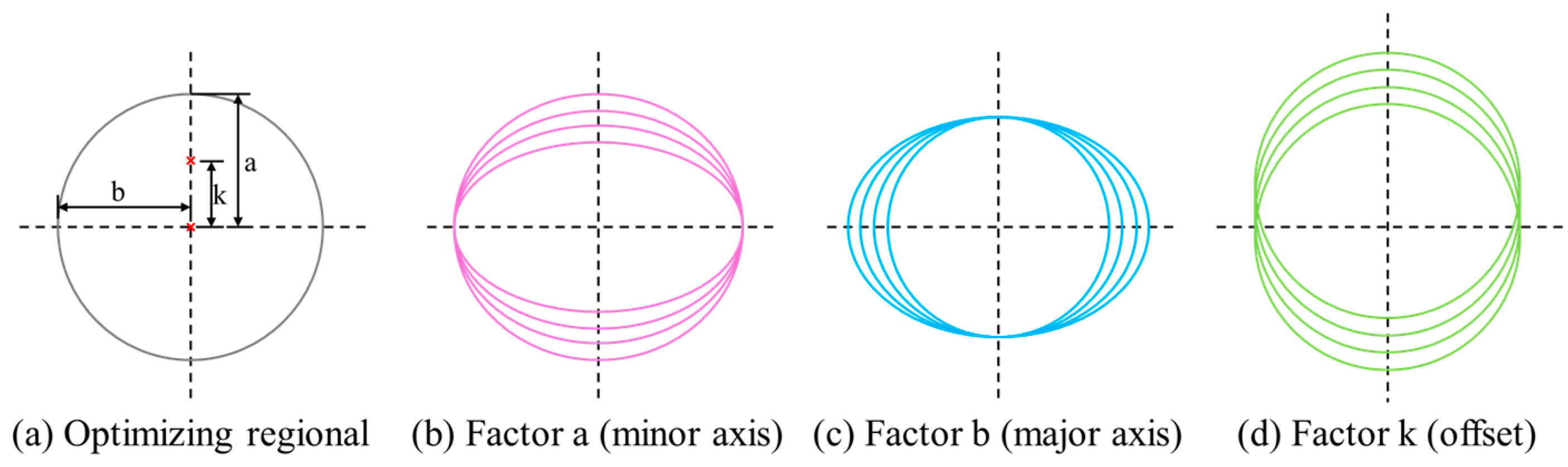
The ranges of the design variables were determined through a pre-screening procedure to ensure geometric feasibility and numerical reliability. Candidate geometries that caused geometric invalidity or interference, such as self-intersection or blockage of the flow passage, were excluded. In addition, the bounds were finalized to allow generation of meshes satisfying a minimum orthogonal quality greater than 0.05 across the computational domain, enabling consistent convergence and fair CFD-based comparisons. The position of the guide vanes varied from 70 mm to 100 mm from the center of the bend radius to observe the flow performance as a function of position. In addition, the angle of the guide vane tip from the bend exit was set to range from 1° to 30° to quantitatively evaluate the change in flow at different angles. Details of the range of design parameters for the guide vane are shown in Figure 5 and

Table 3. Range of parameters of guide vane.

Variable	Value
R [m]	0.07~0.1
$\alpha$ $[°$]	1~30

. The design variables related to nature inspired are the major axis radius, minor axis radius, and the offset of the radius of the existing bending curvature from 45°. The major axis radius was varied from 51 mm (102 mm diameter) to 60 mm (120 mm diameter), the minor axis radius was varied from 30 mm (60 mm diameter) to 49 mm (98 mm diameter), and the offset was varied from 100 mm to 80 mm to analyze the effect of geometry variation on flow characteristics, and the details of the design variables are shown in Figure 6 and

Table 4. Range of parameters of nature-inspired optimization.

Variable	Range [mm]
Minor axis, a	40~49
Major axis, b	51~60
Offset, k	80~90

.

4.2. Response Surface Method

To investigate the effect of the design variables identified in the analysis, we used the response surface method (RSM) as a sensitivity-analysis tool [26]. Non-parametric regression (NPR) and genetic aggregation (GA) methods were used to generate the response surface. The results calculated by each method were compared to each other to determine the most optimal combination of design variables [27].

4.2.1. Non-Parametric Regression

Non-parametric regression methods determine predicted values for input variables based on design points generated by the experimental design method and can be expressed as follows [26]:

$$Y=⟨W,X⟩+b=\sum _{i=1}^N\left(A_i-A_i^{*}\right)K\left(X_i,\overrightarrow{X}\right)+b$$

(11)

where $W$ is the weight vector and $K\left(X_i,\overrightarrow{X}\right)$ represents the kernel map. $A_i$ and $A_i^{*}$ are the Lagrange multipliers. The model parameters are obtained by solving an optimization problem that minimizes the prediction error between the design-point outputs and the corresponding target values [27]. Accordingly, the Lagrange double formula is adopted and written as:

$$MINL=0.5\sum _{i=1}^N\sum _{j=1}^N\left(A_i^{*}-A_i\right)\left(A_j^{*}-A_j\right)K\left(X_i-X_j\right)$$

(12)

4.2.2. Genetic Aggregation

Furthermore, a response surface model based on genetic aggregation technique was used in parallel to predict complex nonlinear responses more precisely. This method improves the overall response prediction accuracy by constructing various regression-based models (e.g., polynomial regression, NPR, radial basis, etc.) and aggregating the prediction results of each model through genetic algorithm-based weights [28,29]. The final response surface is represented as follows:

$$\widehat{f_{GA}}\left(\overrightarrow{x}\right)=\sum _{k=1}^M{w}_k\cdot \widehat{f_k}\left(\overrightarrow{x}\right)$$

(13)

where $\widehat{f_{GA}}\left(\overrightarrow{x}\right)$ is the prediction result of the individual sub models, and $w_k$ is the weight value optimized by the genetic algorithm. All weights are set to satisfy the following constraints:

$$\sum _{k=1}^M{w}_k=1,\hspace{1em}{w}_k\ge 0$$

(14)

These ensemble-based techniques do not rely on a single model but are organized to minimize the overall prediction error ($RMSE$, $R^2$, etc.), which is effective for improving prediction performance in complex design spaces.

4.3. Genetic Algorithm

In this study, MOGA was used to perform the multi-objective optimization. The method considers multiple objective functions together and searches for Pareto-optimal trade-off solutions [30], which is effective for geometry optimization problems showing nonlinear response characteristics [31]. A practical limitation is that the computational demand increases markedly with the number of design variables because each generation requires repeated objective evaluations over a population [32]. This can restrict the number of generations that can be executed within available resources and, in turn, affect the extent of Pareto-front exploration. In order to address this limitation, in this study, we used LHS to improve the quality and diversity of the initial generation during the initialization of the design variable space. This approach allowed us to ensure that the solutions were evenly distributed throughout the design space during the initial exploration phase, which improved the performance of the global search and made more efficient use of computational resources. Based on this approach, we performed optimization under the following conditions:

$$\begin{array}{c}Find a, b, k, \alpha , R\hfill \\ To maximize velocity uniformity\hfill \\ To minimize total pressure drop coefficient, K\hfill \\ For range of design variables detailed in Tables 3 and 4\hfill \end{array}$$

(15)

5. Results and Discussion

5.1. Results of Numerical Simulation

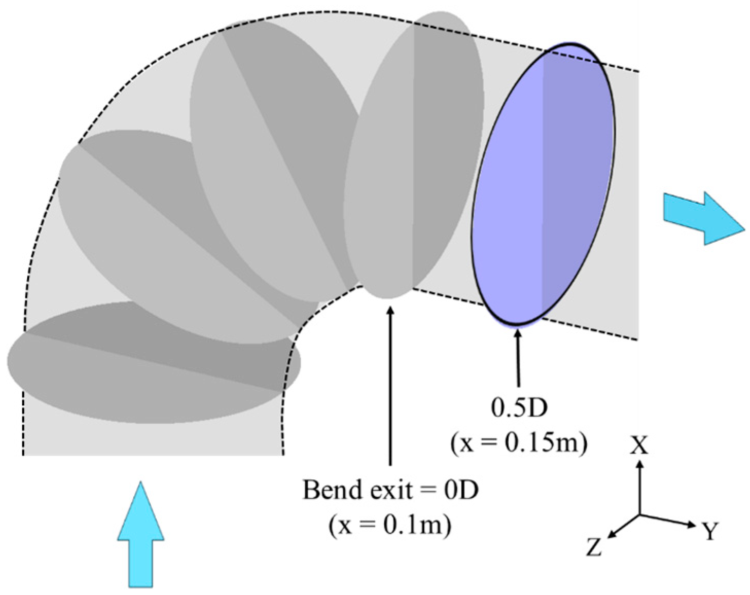
A total of 50 design points were obtained for five design variables using Latin hypercube sampling. The objective functions were defined as the total pressure drop coefficient and the velocity uniformity at 0.5D (x = 0.15 m), as illustrated in Figure 7. Numerical analysis was performed for each design point to calculate the value of the objective function, and based on this, a response surface model was constructed using non-parametric regression (NPR) and genetic aggregation (GA) and used in the optimization process.

5.2. Results of RSM

The response surface was evaluated by comparing observed (x-axis) and model-predicted (y-axis) values at the design points. Observed values were obtained from the simulations, and predicted values were generated by the NPR and GA surrogate models trained using the observed data. This comparison is an important criterion for validating the prediction accuracy and evaluating the reliability of the response surface model to be used in the optimization process. A tighter clustering of points around the diagonal line reflects higher predictive accuracy. The fit of the response surface was evaluated quantitatively by calculating $R^2$ and RMSE from the NPR- and GA-based predictions. The coefficient of determination, $R^2$, represents the proportion of the variance in the response that is accounted for by the regression model. An $R^2$ value of 1 indicates a perfect fit of the response surface to the data. Accordingly, response-surface quality improves as $R^2$ approaches 1 and the root mean square error approaches 0:

$$R^2=1-{\displaystyle \frac{{\sum }_{i=1}^N{\left(y_i-\widehat{y_i}\right)}^2}{{\sum }_{i=1}^N{\left(y_i-\overline{y}\right)}^2}}$$

(16)

$$RMSE=\sqrt{{\displaystyle \frac{1}{N}}\sum _{i=1}^N{\left(y_i-\widehat{y_i}\right)}^2}$$

(17)

where $\widehat{y}$ denotes the predicted value of y, and $\overline{y}$ denotes the average value of y.

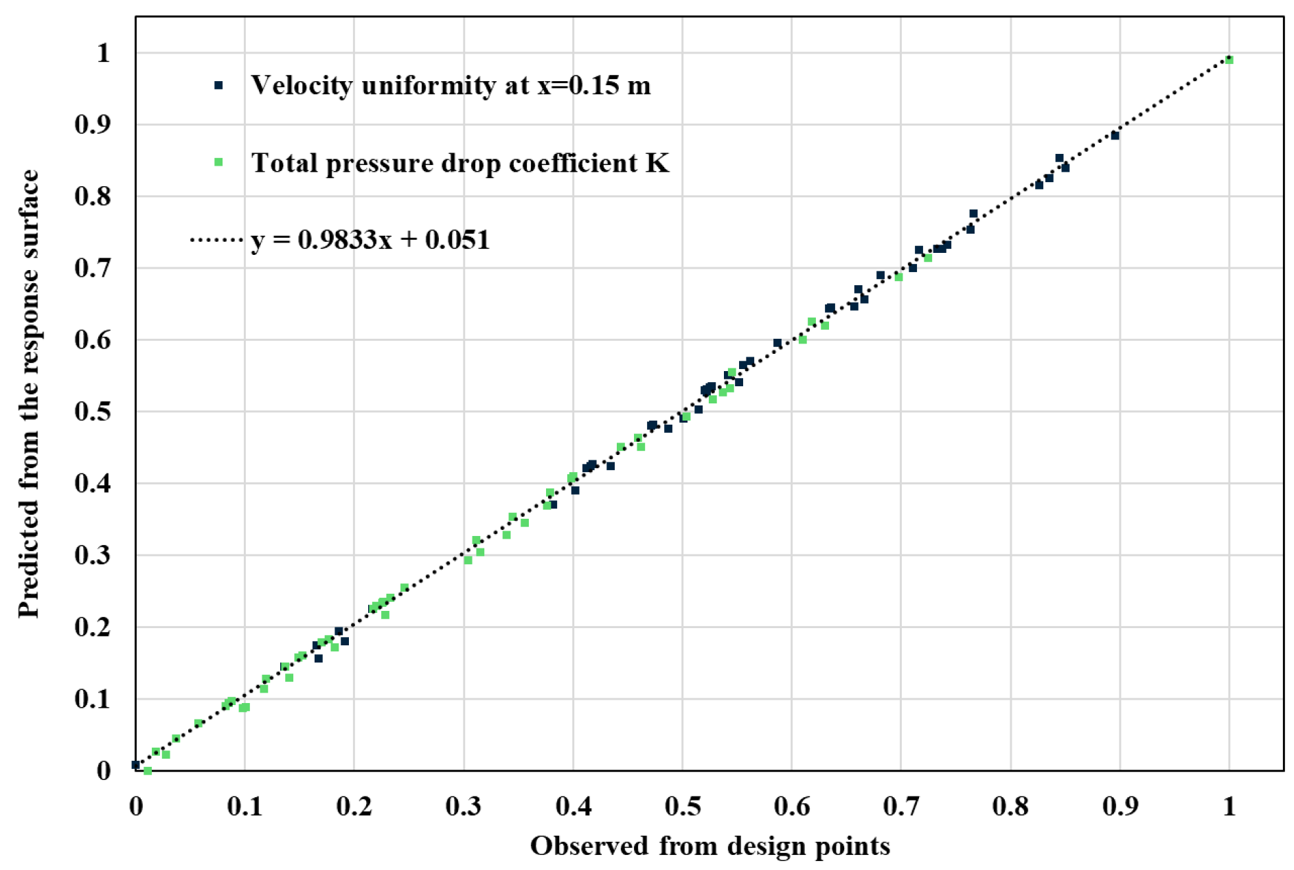
Figure 8 shows a graph comparing observed and predicted values using NPR, which approximates a linear correlation between the predicted values and observed ones, resulting in the following trend line:

$$y=0.9833x+0.051$$

(18)

A trend line with a slope close to 1 and a y-intercept close to 0 means that the model’s predictions are in good agreement with the actual observed values. For NPR, the slope of the trend line is 0.9833, which is close to 1, meaning that as the observed value changes, the predicted value changes at about the same rate. The y-intercept is 0.051, which is close to 0, indicating that there is no significant bias in the model. Of the two outcome variables, the coefficient of determination, $R^2$, for velocity uniformity is 0.99806 with a root mean square deviation, RMSE, of 0.0014735, and $R^2$ for total pressure drop coefficient (K) is 0.9981 with a root mean square deviation of 0.007431. This indicates that the quality of the response surface generated by NPR for the two outcome variables is validated.

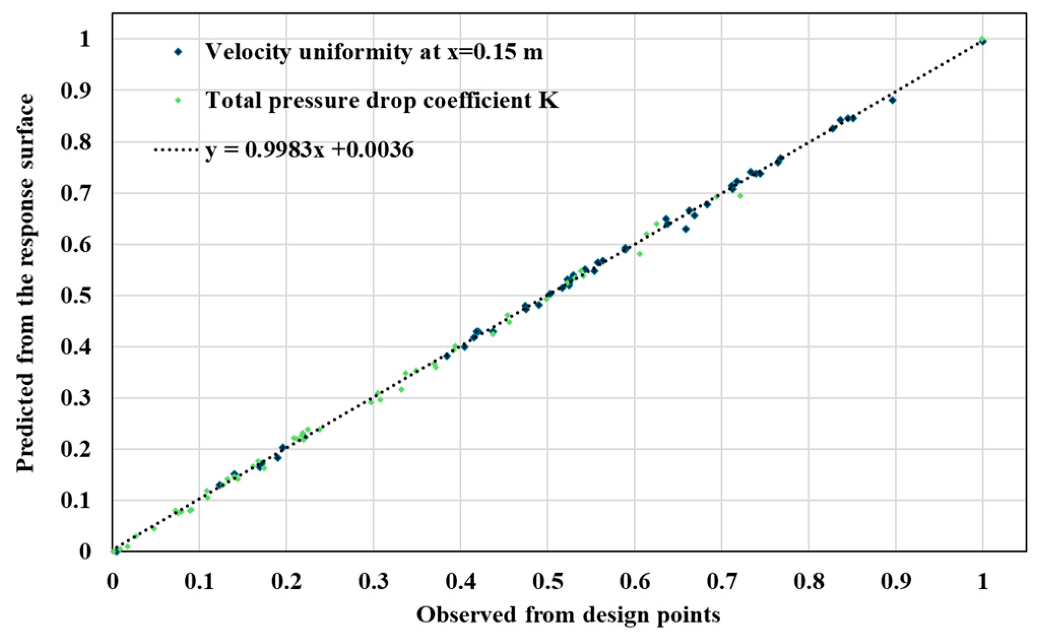
Figure 9 is a graph comparing observed and predicted values using GA, which approximates a linear relationship between the predicted values and observed ones, resulting in the following trend line:

$$y=0.9983x+0.0036$$

(19)

The slope of the trend line is 0.9983, which is close to 1, meaning that as the observed values change, the predicted values change at about the same rate. The y-intercept is 0.0036, which is close to 0, indicating that there is no significant bias in the model. Of the two outcome variables, $R^2$ for velocity uniformity is 0.99883 with an RMSE of 0.0011426, and $R^2$ for total pressure drop coefficient is 0.99828 with an RMSE of 0.0070706. This indicates that the quality of the GA-generated response surface for the two outcome variables is validated.

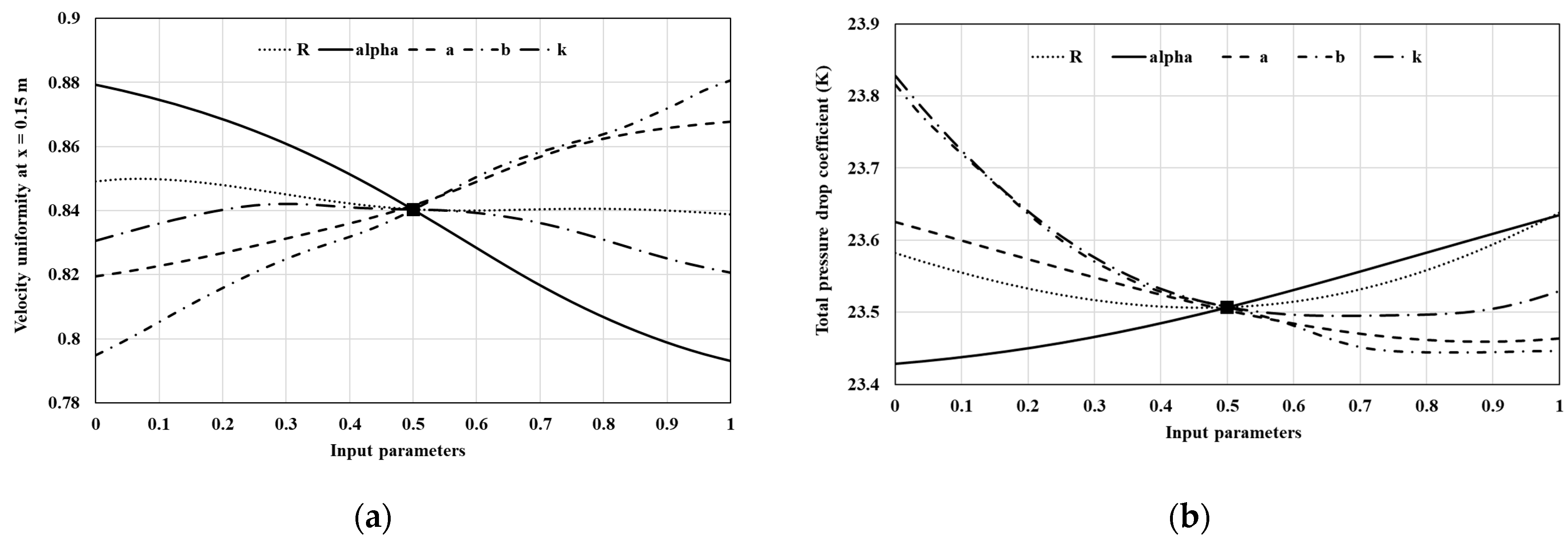
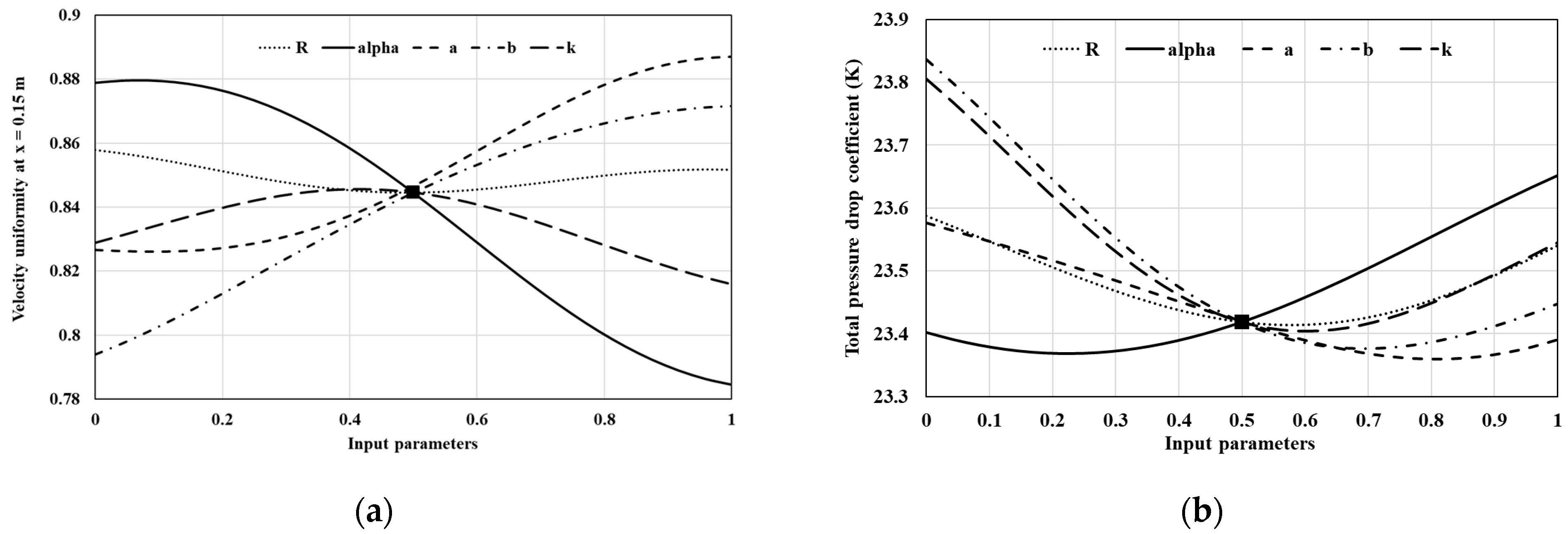
Based on the two qualitatively validated response surface models, the sensitivity of the outcome variable to the input variables is shown in Figure 10. Sensitivity analysis quantitatively identifies the magnitude and direction of the effect of each design variable on the objective function, providing important insights and criteria for determining which variables should be focused on more during the optimization process [33].

Figure 10a shows the sensitivity of the input variables to the velocity uniformity on the response surface using NPR. For the input variables related to the guide vane, the velocity uniformity decreased as the position of the guide vane (R) moved away from the center of the rotation radius and then increased again with a minimum value at 0.5. For the angle from the bend exit of the guide vane ($\mathsf{\alpha }$), the velocity uniformity decreased as the value increased. For the variables related to the nature-inspired geometry, the velocity uniformity increased as the offset from the existing bend radius (k) increased and then decreased again after 0.4. For the major axis (a), the velocity uniformity increased with increasing values, while the minor axis (b) showed the same trend but with a larger slope than the major axis. Figure 10b shows the sensitivity of the input variables to the total pressure drop coefficient (K) on the response surface using NPR. As R increases, K decreases and then increases again after 0.6, and as $\mathsf{\alpha }$ increases, it decreases slightly and then increases again after 0.2. Also, as the offset k increases, K decreases and then increases again after 0.6. For a and K tended to decrease with increasing values of a and increase again after 0.8, while b showed a similar trend but with a larger slope than a, decreasing after 0.65 and increasing again after 0.2.

Figure 11a shows the sensitivity of the input variables to the velocity uniformity on the response surface using GA. For the input variable R related to the guide vane, the velocity uniformity showed relatively small changes compared to the other variables, but for $\mathsf{\alpha }$, the velocity uniformity decreased steeply as the value increased. For the input variable k, which is related to nature inspired, the velocity uniformity increased slightly as the value increased and then decreased after 0.3. For a and b, the velocity uniformity increased as the value increased, especially for b, which showed a larger change. Figure 10b is the sensitivity of the input variables to the total pressure drop coefficient (K). The sensitivity analysis of the total pressure drop coefficient in the genetic aggregation model shows that it decreases with increasing R, has a minimum value at 0.5, and then tends to increase again. For $\mathsf{\alpha }$ and K also tended to increase moderately as the value increased. For the variable k, which is related to the nature inspired shape, K decreased as the value increased, with a minimum value of 0.67, and then tended to increase again. The geometric parameters, a and b decreased as the value increased, with the effect of b being stronger than that of a. The sensitivity analysis for $\mathsf{\alpha }$ showed that K also tended to increase moderately as the value increased.

The results of the sensitivity analysis of the response surfaces using NPR and GA were similar to each other. This similarity suggests that both models effectively capture complex nonlinear relationships and are consistent in their predictions. Both results also suggest that there are trade-offs between each variable. For the input variables related to the guide vane, the trade-off between velocity uniformity and total pressure drop coefficient shows that for $\mathsf{\alpha }$, the velocity uniformity is maximized at 0.1, but the total pressure drop coefficient does not show a minimum at the same point, indicating a trade-off between the two objective functions. Also, for R, the velocity uniformity is maximized at 0, but the total pressure drop coefficient does not have a minimum at the same point. The nature inspired input variables also have different locations for the maximum value of velocity uniformity and the minimum value of total pressure drop coefficient, which clearly shows the trade-off between the design variables. Therefore, to account for these trade-offs, a multi-objective optimization design is required to explore how the input variables influence the responses and to simultaneously optimize velocity uniformity and the total pressure drop coefficient.

5.3. Results of Genetic Algorithm

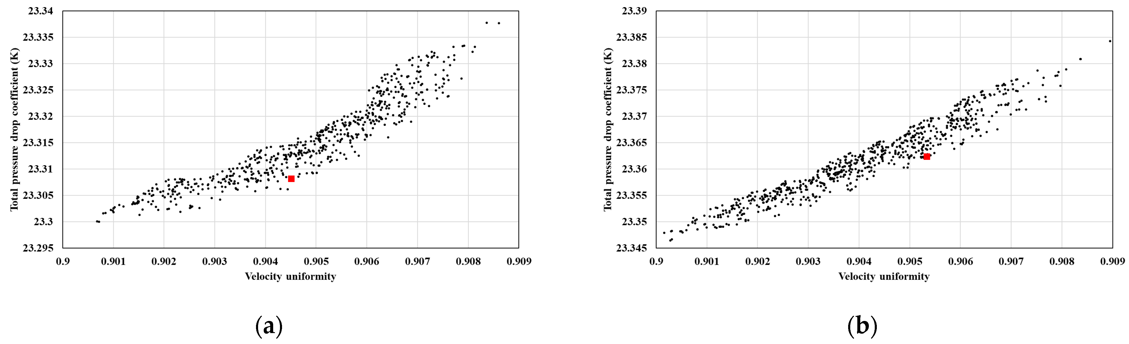
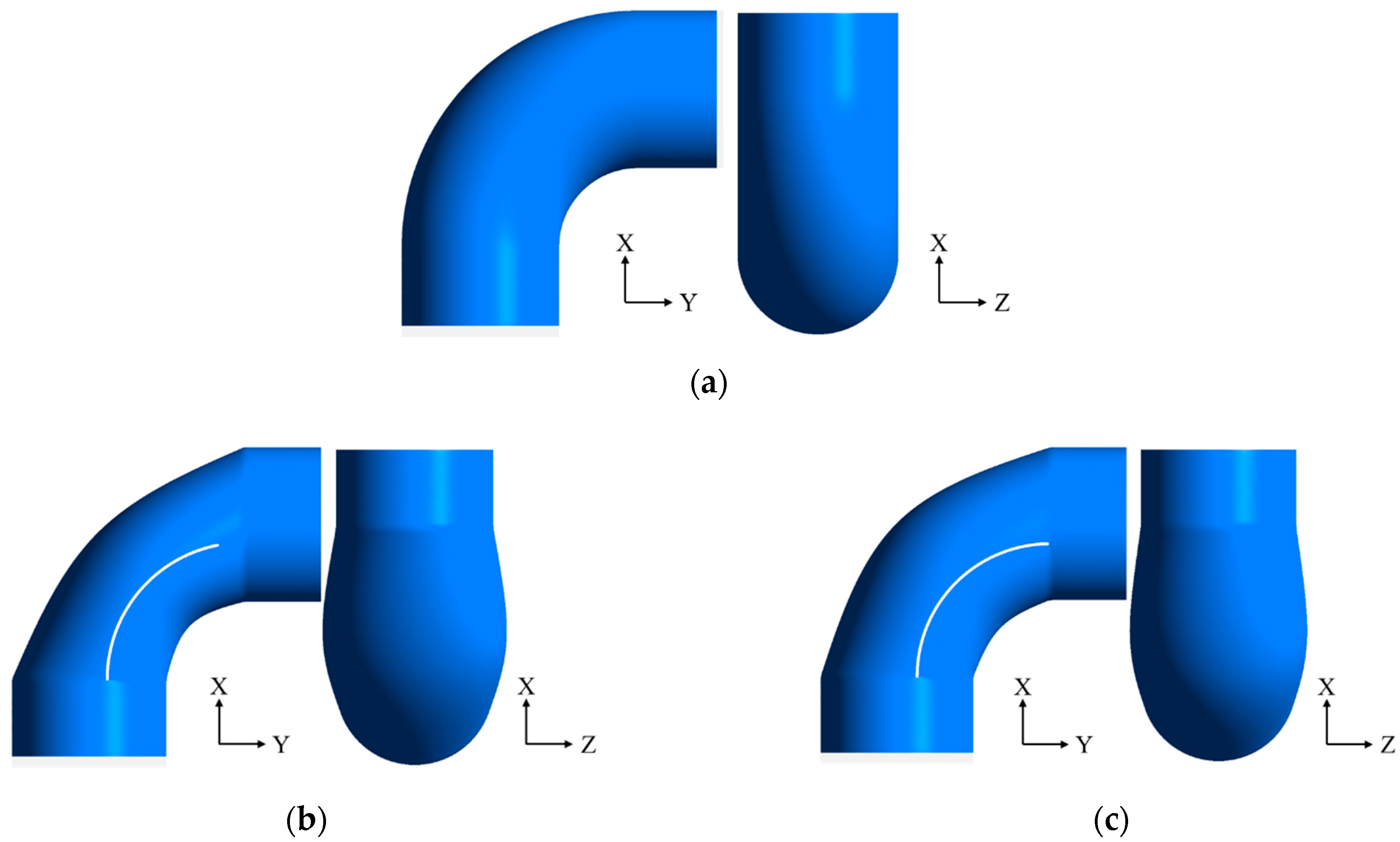
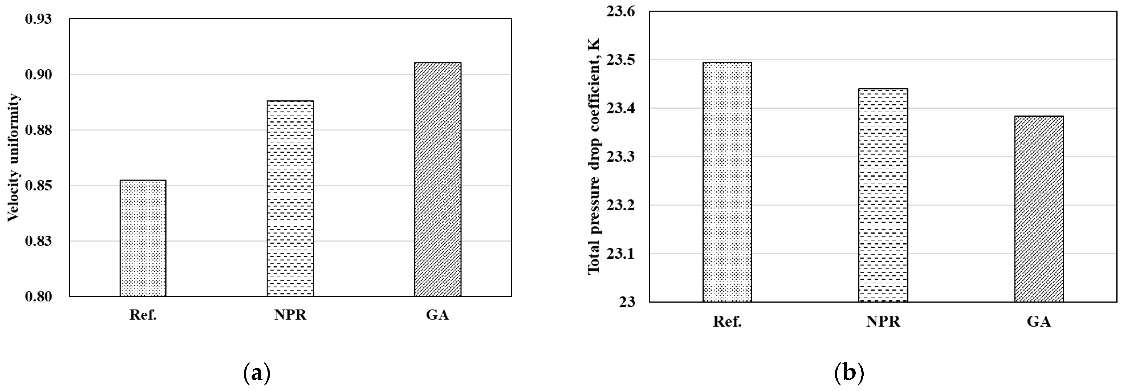
The goal of multi-objective optimization is to find the set of Pareto optimal solutions, called the Pareto front. The Pareto curve results are shown in Figure 12. The black points on the Pareto curve, which are the set of solutions that result from considering the relationship between velocity uniformity and the total pressure drop coefficient. The optimal points selected from the set are colored in red, and CFD was performed with the input variables of each optimal point to validate the optimal points. The simulation results show that the velocity uniformity is 0.8881 and the total pressure drop coefficient is 23.4396 for the case using NPR. Compared to the predicted results, the errors are 1.81% and −0.56%, respectively. For the case using GA, the velocity uniformity is 0.9051 and the total pressure drop coefficient is 23.3829, with errors of 0.03% and −0.09% compared to the predicted results, respectively. Both cases are consistent within 5%, so they can be verified as optimal. The geometries of each elbow are shown in Figure 13, and the detailed dimensions of the design parameters of the optimized elbow are shown in

Table 5. Detail geometry of optimized elbows.

	GA	NPR
R	87.876	89.303
$\mathsf{\alpha }$	1.030	11.021
a	56.961	58.533
b	48.248	42.439
k	93.573	91.433

. The velocity uniformity and total pressure drop coefficient of the verified optimal model and the reference geometry are compared and shown in Figure 14 and

Table 6. Comparison of results between the reference elbow and optimized elbows.

Case	Velocity Uniformity	Total Pressure Drop Coefficient (K)
Ref.	0.85238659	23.493331
NPR	0.88809505	23.439604
GA	0.90511204	23.382878

. The velocity uniformity of the NPR-optimized geometry is improved by 4.021%, and the total pressure drop coefficient is reduced by 0.229% compared to the reference geometry. The velocity uniformity of the GA-optimized geometry is improved by 5.825%, and the total pressure drop coefficient is reduced by 0.470% compared to the reference geometry.

5.3.1. Flow Visualization

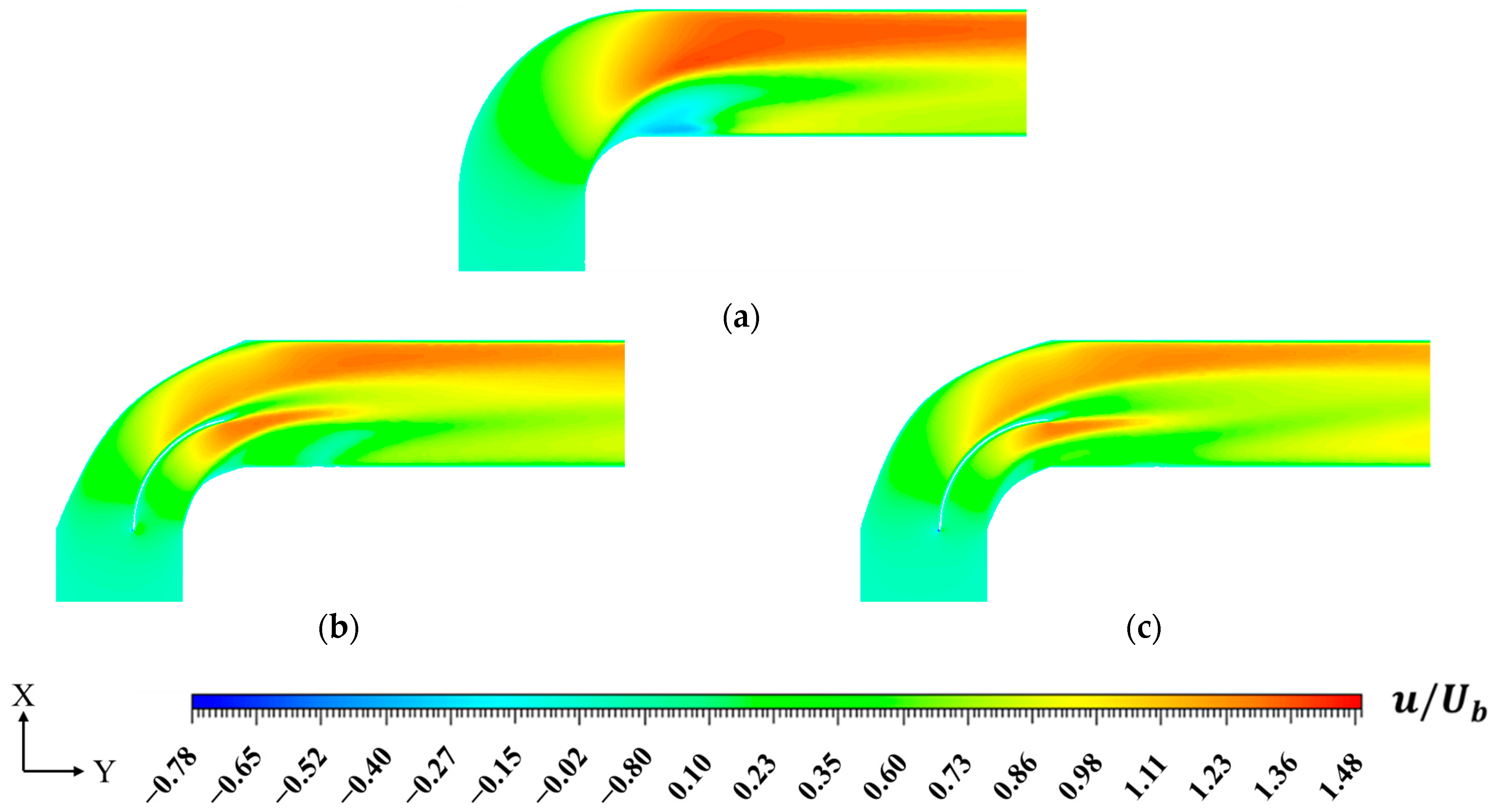
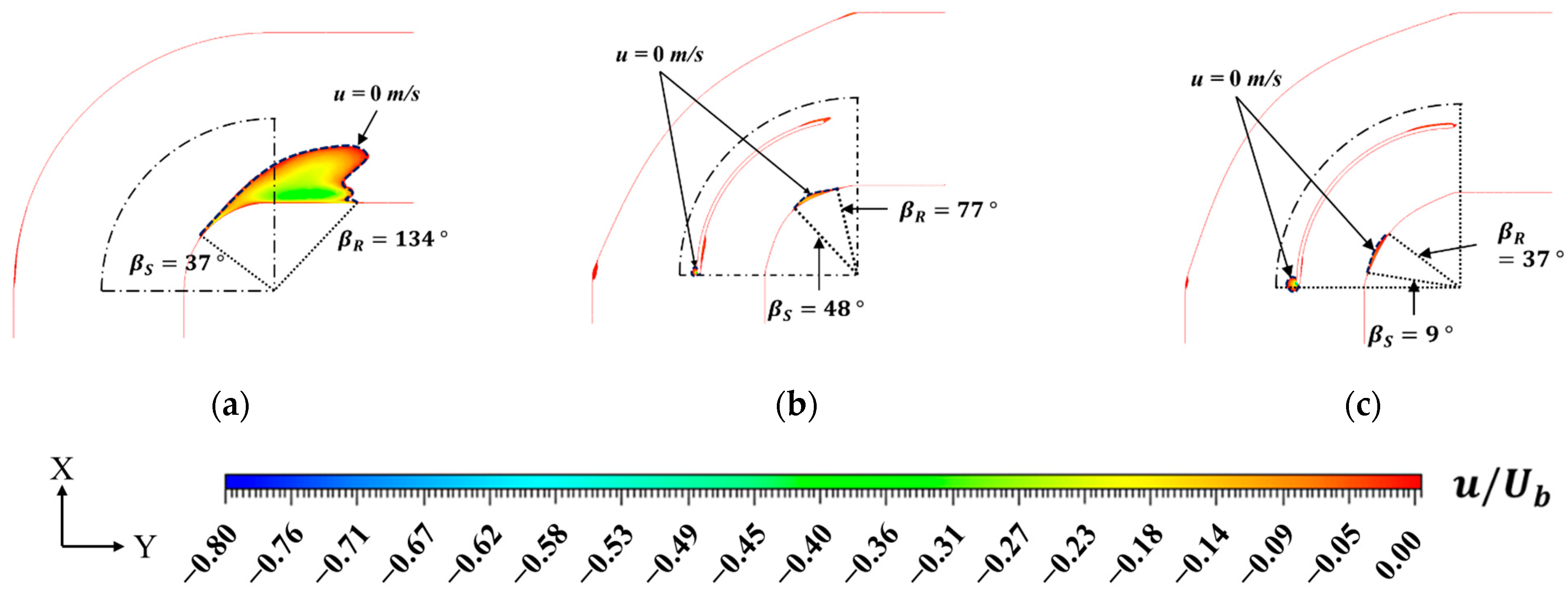
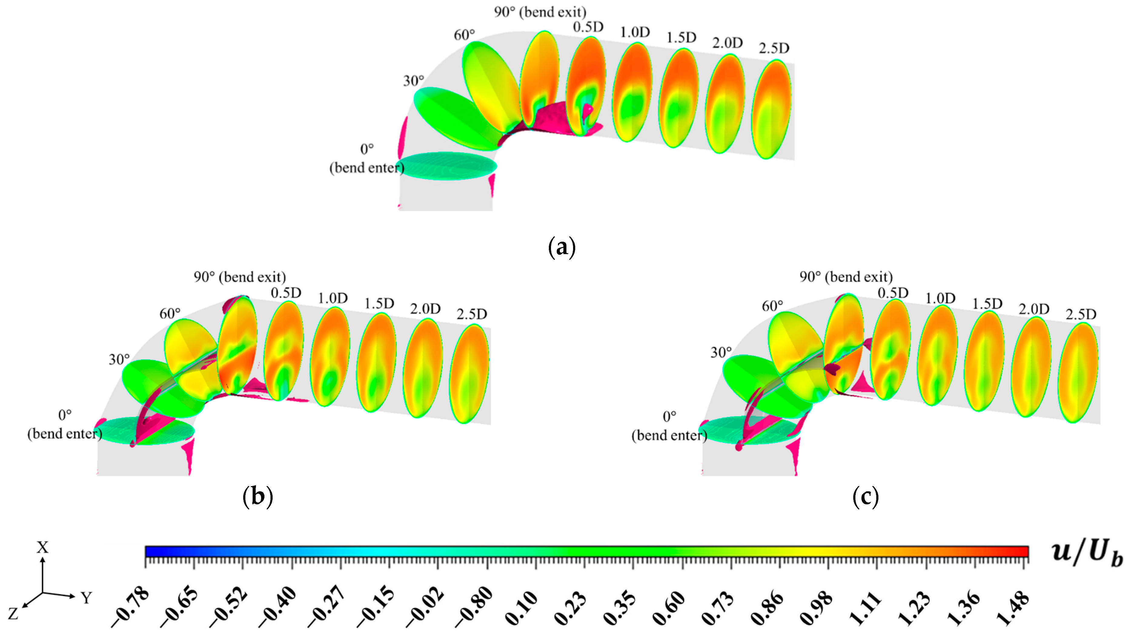
To evaluate the effect of the optimized elbow shape, the axial velocity distribution along the symmetry plane (z = 0) is shown in Figure 15. From this comparison, the effect of the guide vane and elbow shape on the flow can be evaluated, focusing in particular on the change in the velocity distribution within the flow field. The maximum axial velocity reaches $u/U_b=1.48$, which is 48% higher than the velocity of 1 m/s in the inlet. However, the imbalance in the pressure distribution is caused by the centrifugal force acting on the fluid as it passes through the bend. This force creates a radial pressure gradient, resulting in higher pressure along the outer wall and lower pressure along the inner wall. As a result, the pressure imbalance induces secondary flow, which causes cross-sectional vortex motion within the bend. For the reference model without the guide vane and nature inspired, the flow separation point (S) occurred at ${\mathsf{\beta }}_S=37°$. This is a very similar value to the location of the flow separation point (S) observed in the elbow without guide vane in the study of [3]. For the optimized elbow in this study, the NPR occurred at ${\mathsf{\beta }}_S=48°$ and the GA occurred at ${\mathsf{\beta }}_S=9°$. The flow reattachment point (R) represents the location where fluid accumulates and causes disturbances and drops and plays an important role in the behavior of the secondary flow regime. For the reference model without guide vane, the flow reattachment point (R) was observed at x=0.15 m (${\mathsf{\beta }}_S=134°$). This is similar to the flow reattachment point (R) observed for the elbow without guide vane in [3]. For the optimized elbows, flow reattachment occurred at ${\mathsf{\beta }}_R=77°$ for the NPR, and flow reattachment occurred at ${\mathsf{\beta }}_R=37°$ for the GA. For both optimized elbows, flow detachment and reattachment occurred within 30° of the change in $\mathsf{\alpha }$ within the band, which is shown in Figure 16. These results highlight that the optimized elbow geometry is effective in significantly reducing backflow and improving flow uniformity within the system. Figure 17 shows the axial velocity distribution at different points in the elbow and downstream, visualizing the backflow region through an iso-surface with $u = -0.001 \mathrm{m}/\mathrm{s}$. For the reference elbow, backflow regions are observed downstream from the inside of the bend, but for the optimized elbow, these backflow regions are significantly reduced, indicating that flow delamination is suppressed and overall flow efficiency is improved.

5.3.2. Axial Vorticity

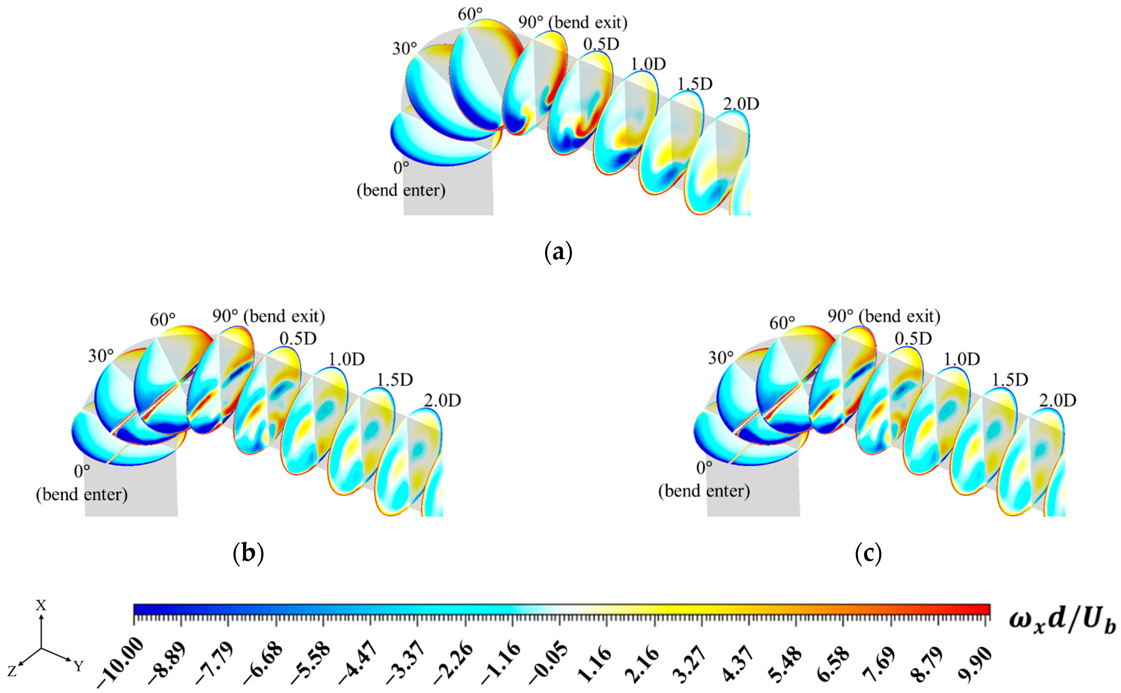
The elbow flow is characterized by curvature-induced secondary motion that arises from the imbalance between centrifugal forces and the cross-stream pressure gradient, leading to a pair of counter-rotating Dean vortices in the cross-section. To quantify the strength of this secondary flow, Figure 18 presents the dimensionless axial vorticity, which represents the streamwise rotation about the x-axis and is commonly used to identify Dean vortex structures. For the reference elbow, the vorticity field is mainly concentrated within the bend and remains pronounced downstream, indicating sustained secondary-flow activity after the turn. In contrast, both optimized cases show a clear attenuation of axial vorticity, implying a weakened Dean vortex. This reduction is attributed to the combined effects of the guide vane and the nature-inspired cross-sectional morphing. The guide vane promotes streamline alignment through the bend and suppresses cross-stream migration that feeds the vortex cores, while the modified cross-section mitigates the curvature-driven pressure-gradient distribution that drives secondary-flow formation. Quantitatively, at 1.0D downstream from the elbow outlet (x = 0.2 m), the axial vorticity decreases from 160.013 in the reference case to 101.23 for NPR and 65.008 for GA, corresponding to reductions of 36.74% and 59.37%, respectively. The weakened secondary-flow intensity is expected to reduce mixing-related losses and contribute to the overall pressure-loss reduction observed in the optimized elbows.

5.3.3. Turbulent Kinetic Energy

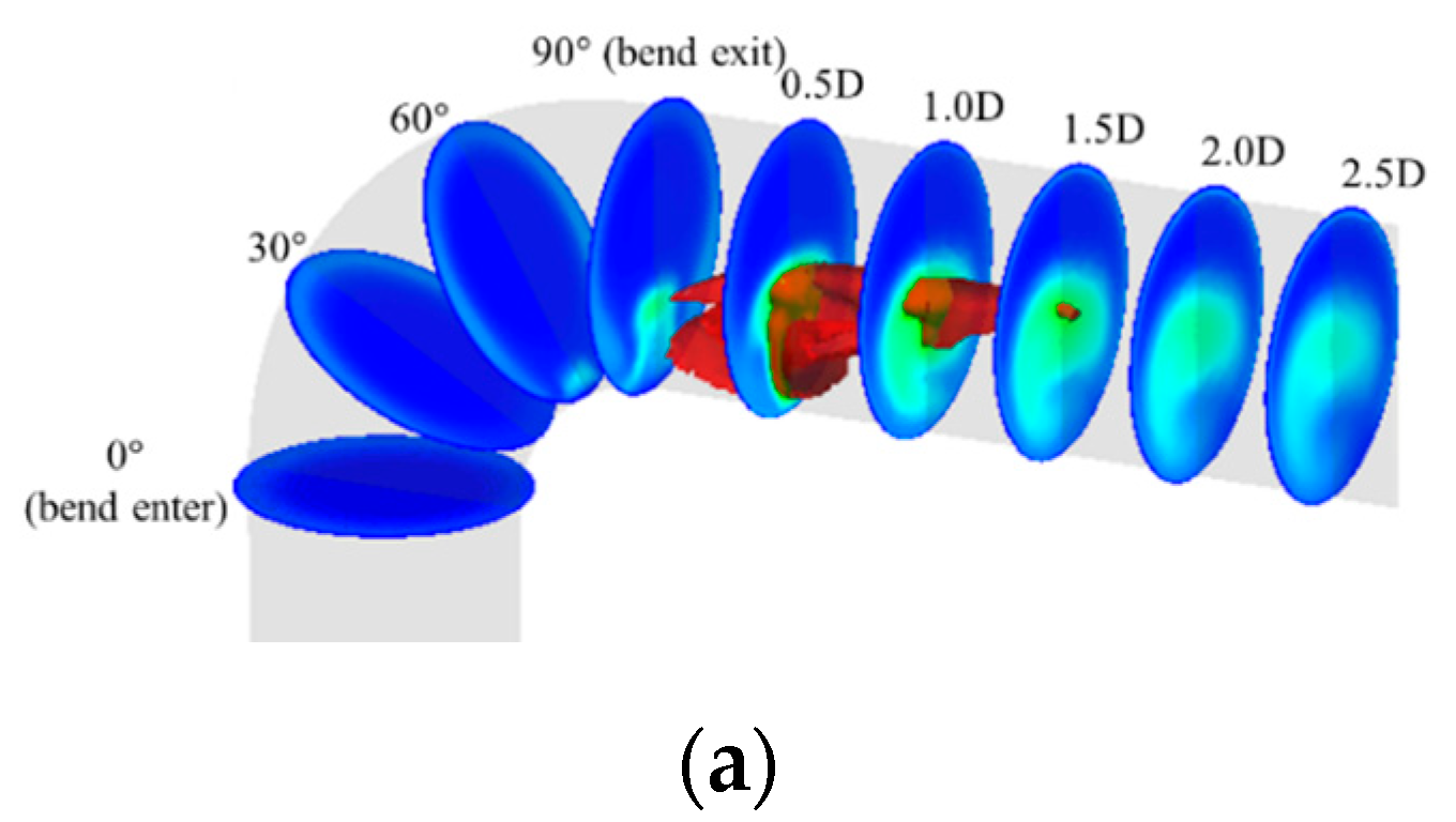
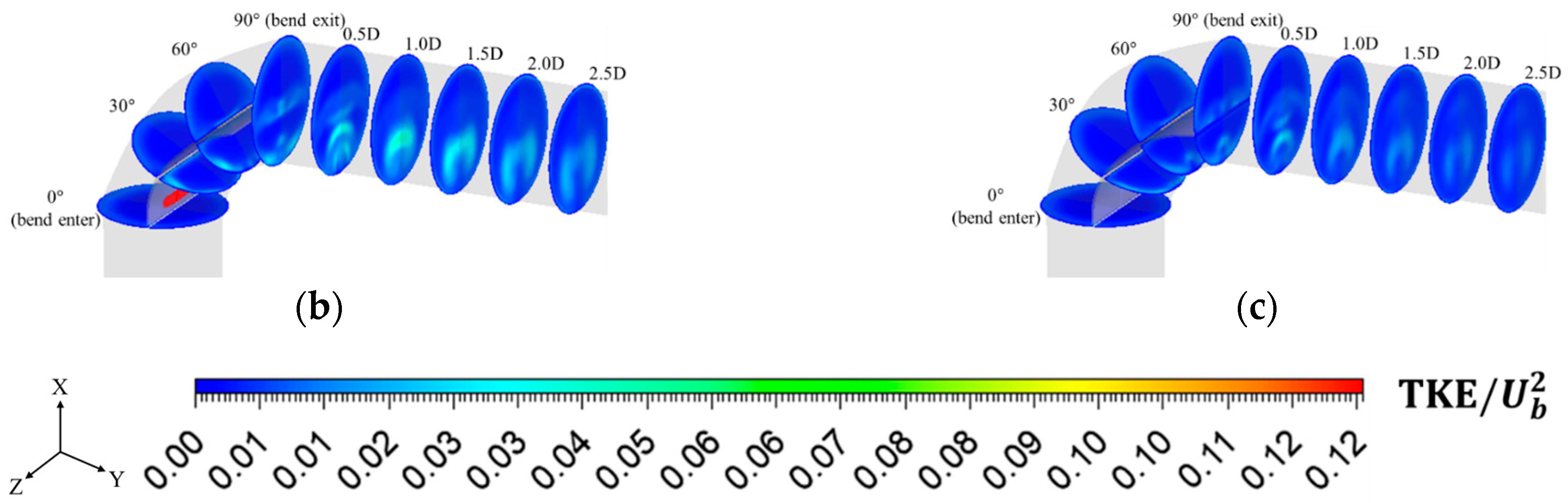
Turbulent kinetic energy (TKE) represents the intensity of turbulent fluctuations associated with eddies and vortical motions. In the present elbow flow, a pronounced high-TKE region appears near the inner wall. This trend is attributed to the strong acceleration along the inner wall in the first half of the bend and the subsequent separation in the second half, which produces a shear layer and promotes turbulent production. To visualize the spatial development of turbulence, Figure 19 shows contours of $\mathrm{T}\mathrm{K}\mathrm{E}/U_b^2$ in the bend and downstream region, together with an iso-surface of $\mathrm{T}\mathrm{K}\mathrm{E}/U_b^2=0.06$. Compared with the reference elbow, the optimized elbows exhibit a markedly reduced extent and intensity of the high-TKE region, indicating suppressed turbulence growth downstream of the bend. This behaviour can be explained by the combined effects of the guide vane and the nature-inspired cross-sectional morphing. The guide vane aligns the flow and reduces cross-stream motion that strengthens separation-related shear layers, while the modified cross-section alleviates curvature-driven imbalance that promotes secondary flows and mixing. Quantitatively, the reference case reaches $\mathrm{T}\mathrm{K}\mathrm{E}/U_b^2=0.120$, whereas the optimized cases reduce this value to 0.047 for NPR and 0.030 for GA, corresponding to reductions of 60.8% and 70.0%, respectively. The reduced turbulent energy level is consistent with weakened separation and secondary-flow activity, which in turn supports the observed reduction in pressure loss [34,35].

5.3.4. Turbulent Energy Dissipation

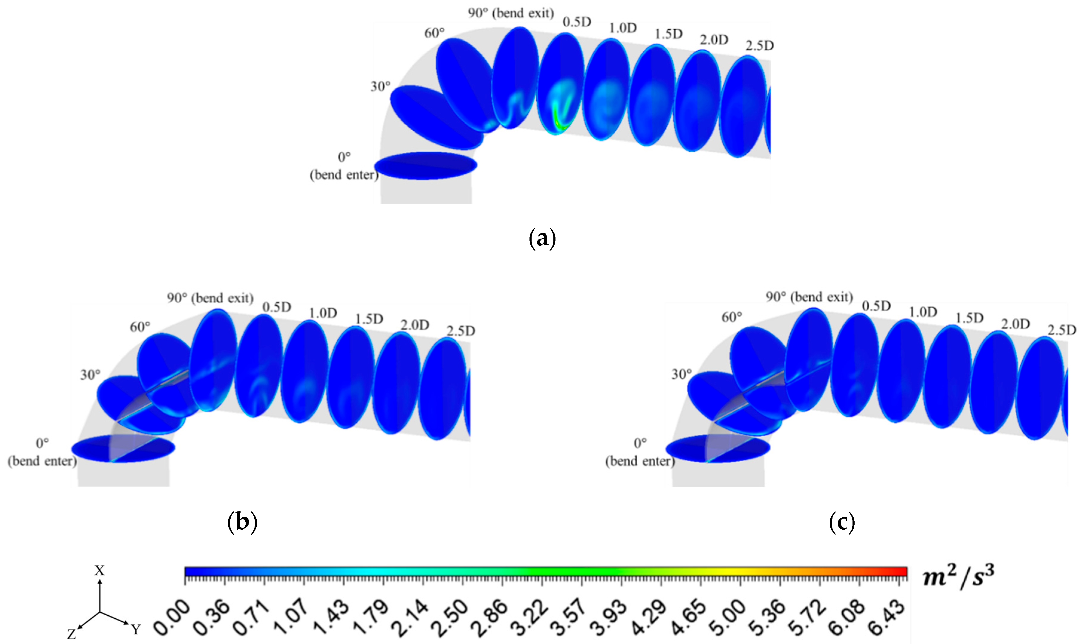
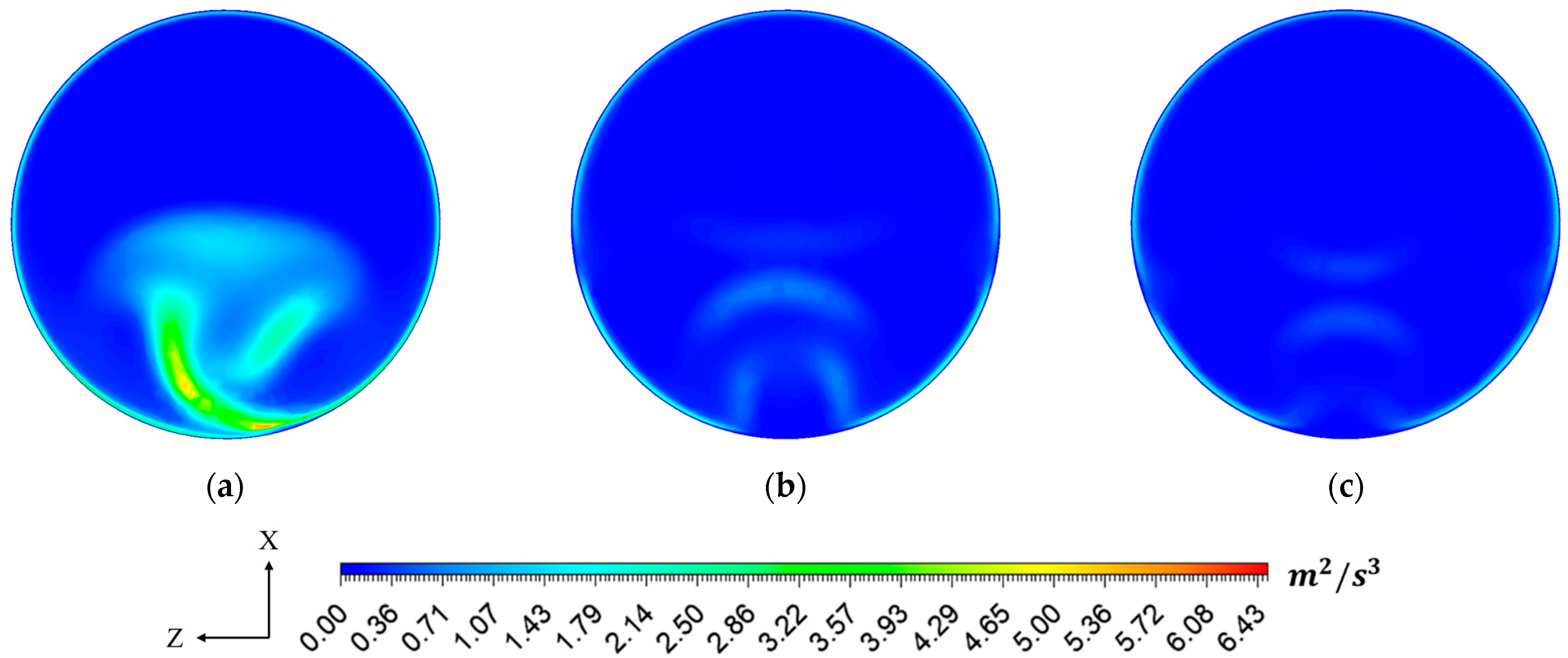
Figure 20 shows the distribution of turbulent energy dissipation on the xy-plane for each elbow. In the reference elbow, the highest dissipation occurs near the inner wall within the bend, which coincides with the separation and recirculation region where strong shear layers and large velocity gradients are formed [3]. In contrast, the optimized elbows exhibit a pronounced reduction in dissipation, indicating that the regions of intense shear and mixing are substantially weakened. This trend is further confirmed in Figure 21, which presents the dissipation contours at 0.5D downstream (x = 0.15 m). Quantitatively, the dissipation level at this location decreases from 8.667 ${\mathrm{m}}^2$/${\mathrm{s}}^3$ in the reference case to 2.383 ${\mathrm{m}}^2$/${\mathrm{s}}^3$ for NPR and 1.686 ${\mathrm{m}}^2$/${\mathrm{s}}^3$ for GA, corresponding to reductions of 71.34% and 80.55%, respectively. The reduction can be attributed to smoother flow turning achieved by the optimized geometry, which suppresses separation-related shear layers and reduces localized velocity gradients, thereby lowering dissipation and minimizing energy loss [5].

5.3.5. Pressure Distribution

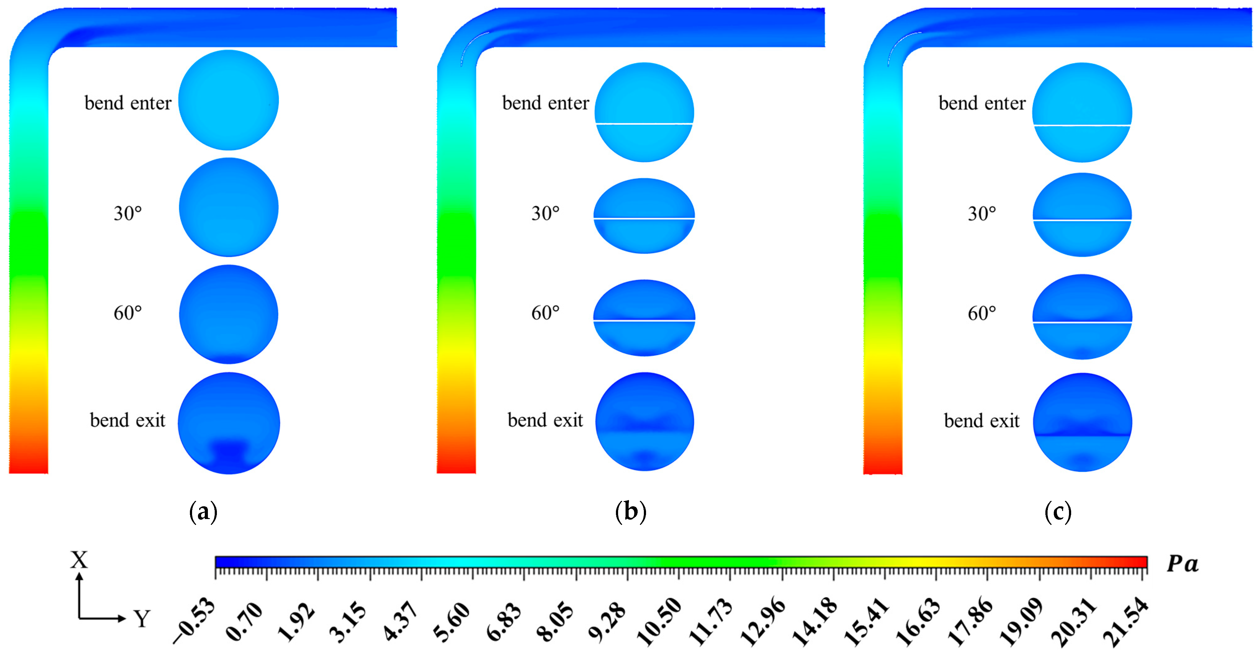
Figure 22 shows the distribution of the total pressure in the xy plane at z = 0 and at 30° intervals from the inlet to the outlet of the bend. The total pressure distribution clearly shows the flow acceleration and deceleration regions and the resulting pressure changes. According to existing studies, near the inner wall of the elbow, flow separation can cause low and even negative pressure, and adding a guide vane can alleviate this pressure imbalance, reduce flow separation, and reduce the static pressure on the outer wall [5]. For the reference elbow, the flow separates from the wall as it passes through the bend, resulting in an uneven distribution of pressure at the bend exit, which can be seen in Figure 22. However, the optimized elbow shows a more uniform pressure distribution than the reference elbow as it passes through the guide vane. This is because the guide vane contributes to redistributing the flow and alleviating the pressure gradient, which improves the overall flow stability [35].

5.4. Comparison Between Non-Parametric Regression and Genetic Aggregation Models

During the optimization process, NPR and GA response surface models were used to accurately predict the complex relationships between the design variables and the objective function. A comprehensive comparison of these two models shows that GA performs better than NPR in both prediction accuracy and final optimization results. The results of comparing the quality of the response surfaces are shown in

Table 7. Comparison of coefficients of determination and root mean square deviation between NPR and GA.

Model	Velocity Uniformity		Total Pressure Drop Coefficient (K)
	${\mathit{R}}^2$	RSME	${\mathit{R}}^2$	RSME
NPR	0.99806	0.001474	0.9981	0.007431
GA	0.99883	0.001143	0.99828	0.007071
Difference	0.08%	22.46%	0.02%	4.85%

and

Table 8. Comparison of slope of trend line and y-intercept between NPR and GA.

Model	Slope of Trend Line	y-Intercept
NPR	0.9833	0.051
GA	0.9983	0.0036
Difference	1.53%	92.94%

.

Table 7 shows the difference in coefficients of determination, $R^2$, and root mean square deviations, RSME, between NPR and GA. The $R^2$ for velocity uniformity is 0.08% higher for GA, with a 22.46% lower RSME. The $R^2$ for the total pressure drop coefficient was 0.02% higher for GA and 4.85% lower for RSME. These results confirm that GA performs slightly better than NPR.

Table 8 shows the difference in the slope and y-intercept of the trend lines for each model. GA has a slope 1.53% closer to 1 and a y-intercept 92.94% closer to 0 than the NPR, demonstrating that the GA exhibits higher fidelity to the observations.

Compared with NPR, GA can provide higher predictive accuracy in this study because it offers greater functional flexibility for capturing strong nonlinearity and variable interactions in the design space. While NPR represents the response using a fixed polynomial structure, GA can adapt to locally different trends and reduce systematic bias when the response surface changes rapidly across the parameter space. This property is advantageous for elbow-shape optimization where the objectives are highly nonlinear with respect to vane parameters and cross-sectional morphing [28,29]. This multi-model aggregation strategy enables GA to learn a wider range of data patterns than NPR, a single-model approach, and to reflect complex nonlinear relationships between variables in a sophisticated manner. This allows GAs to better explore hidden optima within the design space and minimize overall prediction error.

The superior response surface generated by the GA model led to more effective optimization results. As shown in Table 6 and Figure 13, the optimized elbow using GA improved the velocity uniformity by 6.186% and reduced the total pressure drop coefficient by 0.470% compared to the reference elbow. This is a 1.997% improvement in velocity uniformity and a 0.241% reduction in total pressure drop coefficient compared to the NPR results. Axial vorticity was reduced by 22.64% compared to 36.74% of NPR, turbulent kinetic energy was reduced by 9.2% compared to 60.08% of NPR, and turbulent energy dissipation was reduced by 9.21% compared to 71.34% of NPR. These improvements confirm that GA was more effective in suppressing secondary flow within the hydrogen pipeline elbow, reducing flow separation, and improving overall flow uniformity. In the end, both NPR and GA provided valuable insights, but GA was more effective in accurately modeling the complex hydrogen flow in the optimized elbow, which led to a design that substantially improved the transport performance of the hydrogen pipeline.

5.5. Total Pressure Drop Coefficient of Elbow Variation with Reynolds Number

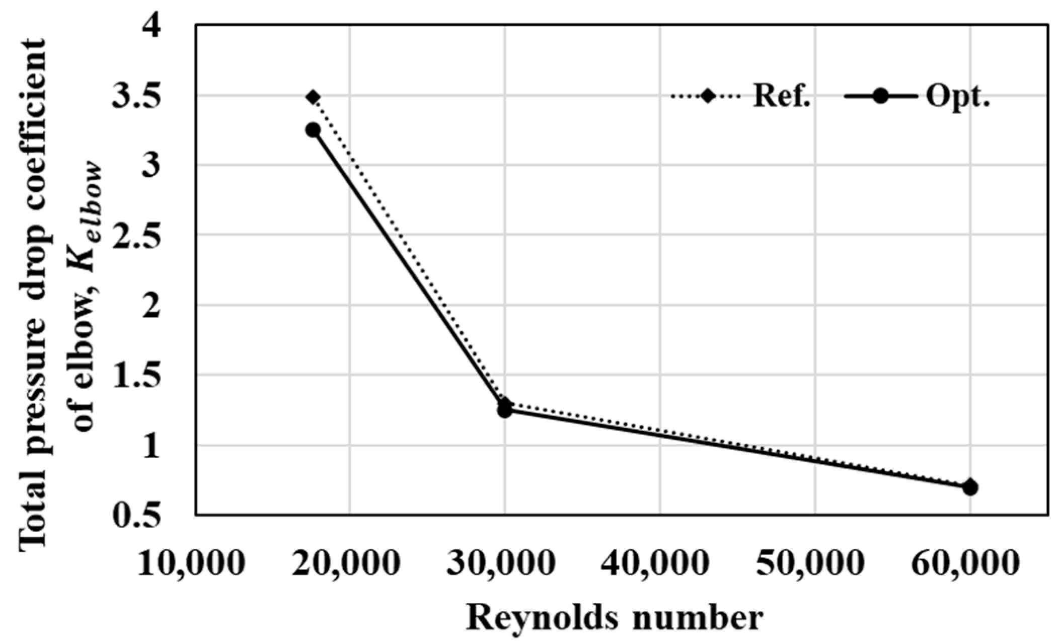
To evaluate the robustness of the optimized geometry under varying operating conditions, the total pressure drop coefficient of the elbow was examined over a Reynolds-number range of Re = 17,600, 30,000, and 60,000. The comparison was conducted between the reference elbow and the optimized elbow obtained using the Genetic Algorithm (GA), which was identified as more effective than NPR in Section 5.4. For each Reynolds number, the inlet bulk velocity was adjusted to match the target Re while preserving the same geometric similarity (r/D) and boundary-condition framework.

Figure 23 presents the variation of the total pressure drop coefficient with Reynolds number for both geometries. At Re = 17,600, the reference elbow exhibited a coefficient of 3.481, whereas the optimized elbow showed a reduced value of 3.248, corresponding to a reduction of approximately 6.7%. At Re = 30,000, the coefficient decreased to 1.302 for the reference elbow and 1.254 for the optimized elbow, yielding an improvement of approximately 3.7%. At Re = 60,000, the coefficient further decreased to 0.7153 for the reference elbow and 0.6982 for the optimized elbow, resulting in a reduction of approximately 2.4%. Overall, the total pressure drop coefficient decreases with increasing Reynolds number for both elbows, and the GA-optimized elbow consistently provides a lower value than the reference geometry across the investigated Reynolds-number range. This indicates that the optimized design is not limited to a single operating point but remains beneficial under different flow conditions.

6. Conclusions

In this study, optimization was performed to improve the velocity uniformity of the 90$°$ elbow and reduce the total pressure drop coefficient to improve the transport performance of the pipe. For nature-inspired technology, minor axis (a), major axis (b), and ellipse centering offset (k) were set as design variables, and for the guide vane, radial position (R) and angle from bend exit ($\mathsf{\alpha }$) were set as design variables. The design point was derived through the LHS method, and optimization was performed by generating the response surface using the NPR method and GA method. As a result of the optimization, the velocity uniformity improved by 4.021% for NPR and 5.825% for GA, and the total pressure drop coefficient (K) was reduced by 0.229% for NPR and 0.470% for GA. As discussed in detail in Section 5.4, the genetic aggregation leveraged an ensemble-based approach to more accurately model the complex and nonlinear hydrogen flow characteristics within the design space, leading to superior optimization results. There is a trade-off between the velocity uniformity and total pressure drop coefficient, and as the input variables change, a non-linear relationship between the two variables emerges, requiring a multi-objective design for optimal conditions that balance the input variables. Compared with the reference elbow, the optimized elbow significantly suppressed the flow separation, reduced the axial vorticity by 36.74% and 59.37%, the turbulent kinetic energy by 60.8% and 70.0%, and the turbulent energy dissipation by 71.34% and 80.55% for NPR and GA, respectively, effectively reducing the secondary flow and improving the flow uniformity to achieve more efficient transport performance. In the production and transportation technology of hydrogen, pipes are an indispensable element, but due to the characteristics of hydrogen, its transportation efficiency is lower than other resources. Such advances in transportation performance are expected to contribute to lowering transportation costs and increasing efficiency. Therefore, this research is expected to contribute significantly to improving the sustainability of hydrogen economy industries. In future work, experimental verification of the optimized elbow proposed in this study will be carried out to substantiate the numerical simulation results and lay the foundation for practical industrial applications, especially under high-pressure compressible hydrogen flow conditions.

References

1. Revinova, S.; Lazanyuk, I.; Gabrielyan, B.; Shahinyan, T.; Hakobyan, Y. Hydrogen in energy transition: The problem of economic efficiency, environmental safety, and technological readiness of transportation and storage. Resources 2024, 13, 92. [Google Scholar] [CrossRef]
2. Hoschke, J.; Chowdhury, M.F.W.; Venezuela, J.; Atrens, A. A review of hydrogen embrittlement in gas transmission pipeline steels. Corros. Rev. 2023, 41, 277–317. [Google Scholar] [CrossRef]
3. Yagmur, S. Optimizing 3D guide vanes to minimize secondary flow and energy loss in turbulent flow through a 90− Degree bend. Ocean Eng. 2025, 319, 120219. [Google Scholar] [CrossRef]
4. Tian, A.; Zhang, Y.; Gao, R.; Li, A.; Xuan, Y.; Wang, Y.; Ren, J.; Yu, S.; Xie, X. A low-resistance local component design method based on biomimicry and a random forest model: A pipe elbow case study. Build. Environ. 2024, 254, 111332. [Google Scholar] [CrossRef]
5. Yin, Y.; Li, A.; Wen, X.; Zhang, J.; Zhang, X.; Guo, J.; Li, J.; Zhang, W.; Che, J. Resistance reduction of an elbow with a guide vane based on the field synergy principle and viscous dissipation analysis. J. Build. Eng. 2022, 54, 104649. [Google Scholar] [CrossRef]
6. Tian, Y.; Gao, R.; Jing, R.; Wang, Y.; Li, A.; Dong, X.; Hao, X.; Ji, Z. Topology optimization of bend for reducing the local resistance in a piping and duct system. Build. Environ. 2025, 270, 112508. [Google Scholar] [CrossRef]
7. Sun, C.; Xiao, Z.; Xiao, Y.; Xu, Z.; Cui, W.; Wang, P.; Fang, Z.; Cui, G.; Jia, L. Research on multi-objective optimization method of Z-shaped pipeline structure based on Kriging model. Sci. Rep. 2024, 14, 29573. [Google Scholar] [CrossRef]
8. Reghunathan Valsala, R.; Son, S.; Suryan, A.; Kim, H.D. Study on reduction in pressure losses in pipe bends using guide vanes. J. Vis. 2019, 22, 795–807. [Google Scholar] [CrossRef]
9. Yoshimura, M.; Shimoyama, K.; Misaka, T.; Obayashi, S. Topology optimization of fluid problems using genetic algorithm assisted by the Kriging model. Int. J. Numer. Methods Eng. 2017, 109, 514–532. [Google Scholar] [CrossRef]
10. Zhang, X.; Ye, T.; Jin, G.; Liu, H.; Xuan, L. Multi-objective optimization of bionic guide vanes for flow rectification in elbow pipes based on convolutional neural network—Second-generation genetic algorithm. Phys. Fluids 2025, 37, 075204. [Google Scholar] [CrossRef]
11. Tao, H.-G.; Chen, H.-X.; Xie, J.-L.; Hu, Y.-P. An alternative approach to quantifying fluid flow uniformity based on area-weighted average velocity and mass-weighted average velocity. Energy Build. 2012, 45, 116–123. [Google Scholar] [CrossRef]
12. Yingzhe, H.; Hao, W.; Xiaozhe, Y.; Haoqiang, Z.; Haitao, G.; Yiming, H.; Qiguan, C.; Jinying, X.; Longyu, Z. Comparative Study on Flow Characteristics of Pipeline System Based on CFD. In E3S Web of Conferences; EDP Sciences: Les Ulis, France, 2021; p. 02053. [Google Scholar]
13. Peng, D.-Y.; Robinson, D.B. A new two-constant equation of state. Ind. Eng. Chem. Fundam. 1976, 15, 59–64. [Google Scholar] [CrossRef]
14. Sun, T.; Takbiri-Borujeni, A.; Nourozieh, H.; Gu, M. Application of Peng-Robinson equation of state for modelling the multiphase equilibrium properties in Athabasca bitumen/ethane mixtures. Fuel 2019, 252, 439–447. [Google Scholar] [CrossRef]
15. Faradonbeh, M.R.; Abedi, J.; Harding, T.G. Comparative study of eight cubic equations of state for predicting thermodynamic properties of alkanes. Can. J. Chem. Eng. 2013, 91, 101–110. [Google Scholar] [CrossRef]
16. Kim, J.; Yadav, M.; Kim, S. Characteristics of secondary flow induced by 90-degree elbow in turbulent pipe flow. Eng. Appl. Comput. Fluid Mech. 2014, 8, 229–239. [Google Scholar] [CrossRef]
17. Menter, F.R. Two-equation eddy-viscosity turbulence models for engineering applications. AIAA J. 1994, 32, 1598–1605. [Google Scholar] [CrossRef]
18. Wilcox, D.C. Turbulence Modeling for CFD; DCW Industries: La Canada, CA, USA, 1998; Volume 2. [Google Scholar]
19. Jones, W.P.; Launder, B. The calculation of low-Reynolds-number phenomena with a two-equation model of turbulence. Int. J. Heat Mass Transf. 1973, 16, 1119–1130. [Google Scholar] [CrossRef]
20. Kolesov, E.; Nakaryakov, E. Selection of turbulence model in ventilation modeling for blind stopes. In IOP Conference Series: Earth and Environmental Science; IOP Publishing: Bristol, UK, 2021; p. 012071. [Google Scholar]
21. Menter, F.R.; Kuntz, M.; Langtry, R. Ten years of industrial experience with the SST turbulence model. Turbul. Heat Mass Transf. 2003, 4, 625–632. [Google Scholar]
22. Mozaffari, S.; Cai, S.-G.; Jacob, J.; Sagaut, P. Lattice Boltzmann k-ω SST based hybrid RANS/LES simulations of turbulent flows. J. Comput. Phys. 2024, 514, 113269. [Google Scholar] [CrossRef]
23. Zhang, J.; Wang, D.; Wang, W.; Zhu, Z. Numerical investigation and optimization of the flow characteristics of bend pipe with different bending angles. Processes 2022, 10, 1510. [Google Scholar] [CrossRef]
24. Ikarashi, Y.; Fujisawa, N. Mass transfer measurements and flow separation behavior in a 90° short elbow. Int. J. Heat Mass Transf. 2019, 136, 1106–1114. [Google Scholar] [CrossRef]
25. Helton, J.C.; Davis, F.J. Latin hypercube sampling and the propagation of uncertainty in analyses of complex systems. Reliab. Eng. Syst. Saf. 2003, 81, 23–69. [Google Scholar] [CrossRef]
26. Khuri, A.I.; Mukhopadhyay, S. Response surface methodology. Wiley Interdiscip. Rev. Comput. Stat. 2010, 2, 128–149. [Google Scholar] [CrossRef]
27. Härdle, W. Applied Nonparametric Regression; Cambridge University Press: Cambridge, UK, 1990. [Google Scholar]
28. Viana, F.A.; Haftka, R.T.; Steffen, V., Jr. Multiple surrogates: How cross-validation errors can help us to obtain the best predictor. Struct. Multidiscip. Optim. 2009, 39, 439–457. [Google Scholar] [CrossRef]
29. Acar, E. Various approaches for constructing an ensemble of metamodels using local measures. Struct. Multidiscip. Optim. 2010, 42, 879–896. [Google Scholar] [CrossRef]
30. Marler, R.T.; Arora, J.S. Survey of multi-objective optimization methods for engineering. Struct. Multidiscip. Optim. 2004, 26, 369–395. [Google Scholar] [CrossRef]
31. Zitzler, E.; Deb, K.; Thiele, L. Comparison of multiobjective evolutionary algorithms: Empirical results. Evol. Comput. 2000, 8, 173–195. [Google Scholar] [CrossRef]
32. Said, R.M.; Sallehuddin, R.; Radzi, N.H.M.; Ali, W.F.F.W. Enhanced Jaya Algorithm for Multi-objective Optimisation Problems. Int. J. Adv. Comput. Sci. Appl. 2022, 13, 624–632. [Google Scholar] [CrossRef]
33. Pais-Chanfrau, J.M.; Núñez-Pérez, J.; del Carmen Espin-Valladares, R.; Lara-Fiallos, M.V.; Trujillo-Toledo, L.E. Uses of the response surface methodology for the optimization of agro-industrial processes. In Response Surface Methodology in Engineering Science; IntechOpen: Rijeka, Croatia, 2021. [Google Scholar]
34. Palkovič, A.; Pečený, P.; Teichman, J. Optimization of pressure drop in curved conduits using Ansys DesignXplorer. In MATEC Web of Conferences; EDP Sciences: Les Ulis, France, 2022; p. 00019. [Google Scholar]
35. Luo, J.; Razinsky, E.H. Analysis of turbulent flow in 180 deg turning ducts with and without guide vanes. J. Turbomach. 2009, 131, 021011. [Google Scholar] [CrossRef]
Figure 1. Schematic of modeled pipeline geometry.
Energies 19 00748 g001
Figure 2. Grid system of geometry. (Adjusting the number of grids for grid visibility).
Energies 19 00748 g002
Figure 3. Verification of grid independence.
Energies 19 00748 g003
Figure 5. Schematic of parameters of guide vane optimization.
Energies 19 00748 g005
Figure 6. Schematic of parameters of nature-inspired optimization.
Energies 19 00748 g006
Figure 7. Schematic of position at x = 0.15 m.
Energies 19 00748 g007
Figure 8. Comparison of the predicted value and the observed one with NPR.
Energies 19 00748 g008
Figure 9. Comparison of the predicted value and the observed one with GA.
Energies 19 00748 g009
Figure 10. Local sensitivity analysis results of NPR: (a) Velocity uniformity; (b) total pressure drop coefficient.
Energies 19 00748 g010
Figure 11. Local sensitivity analysis results of GA: (a) Velocity uniformity; (b) total pressure drop coefficient.
Energies 19 00748 g011
Figure 12. Results of Pareto solution using genetic algorithms: (a) Results of Pareto solution using genetic algorithms with NPR; (b) results of Pareto solution using genetic algorithms with GA.
Energies 19 00748 g012
Figure 13. Geometry of reference elbow and optimized elbows: (a) Reference elbow; (b) NPR elbow; (c) GA elbow.
Energies 19 00748 g013
Figure 14. Results of the reference elbow and optimized elbows: (a) Velocity uniformity; (b) total pressure drop coefficient.
Energies 19 00748 g014
Figure 15. Comparison of axial velocity distribution within the bend section z = 0: (a) Reference elbow; (b) NPR elbow; (c) GA elbow.
Energies 19 00748 g015
Figure 16. Comparison of axial velocity u = 0 m/s and flow separate reattachment point: (a) Reference elbow; (b) NPR elbow; (c) GA elbow.
Energies 19 00748 g016
Figure 17. Development of axial velocity with the iso-surface of secondary flow region for u = 0.001 m/s: (a) Reference elbow; (b) NPR elbow; (c) GA elbow.
Energies 19 00748 g017
Figure 18. Comparison of axial vorticity motion in the axial direction: (a) Reference elbow; (b) NPR elbow; (c) GA elbow.
Energies 19 00748 g018
Figure 19. Comparison of the turbulent kinetic energy with the iso-surface contour for T K E / U b 2 = 0.06 : (a) Reference elbow; (b) NPR elbow; (c) GA elbow.
Energies 19 00748 g019aEnergies 19 00748 g019b
Figure 20. Comparison of the turbulent energy dissipation: (a) Reference elbow; (b) NPR elbow; (c) GA elbow.
Energies 19 00748 g020
Figure 21. Comparison of the turbulent energy dissipation at x = 0.15 m: (a) Reference elbow; (b) NPR elbow; (c) GA elbow.
Energies 19 00748 g021
Figure 22. Comparison of the total pressure contour at z = 0 and bend cross-sections: (a) Reference elbow; (b) NPR elbow; (c) GA elbow.
Energies 19 00748 g022
Figure 23. Total pressure drop coefficient variation with Reynolds number.
Energies 19 00748 g023