1. Introduction
Climate change has been identified for many years as a central global challenge; this conclusion is consistently reinforced in successive IPCC assessments, including the 2014 report and the more recent AR6 publication [
1,
2,
3,
4]. Both documents emphasise that stabilising greenhouse gas emissions, particularly CO
2, is essential for limiting future environmental and socio-economic impacts. Similar priorities were reflected earlier in the Kyoto Protocol and the Paris Agreement, where emission reductions became a core element of international climate policy [
2,
3].
Within this context, the transport sector plays a decisive role. Although it is responsible for approximately 22% of global anthropogenic CO
2 emissions, the share attributed to heavy-duty vehicles (HDVs) and specialised machinery is significantly higher than their proportion in the global fleet would suggest [
4]. These vehicles operate under demanding conditions, often with long duty cycles, high loads, and limited opportunities for energy recovery, which translates directly into disproportionately high fuel consumption [
4,
5]. Their role is particularly evident in mining and construction environments, where Non-Road Mobile Machinery (NRMM) powered by internal combustion engines operate round the clock and account for a substantial share of total energy use.
Over the past two decades, both freight activity and the number of HDVs in operation have grown steadily worldwide [
6,
7]. Long-term projections further indicate that global heavy-duty fleets may nearly double by 2040, resulting in marked increases in fuel demand and related emissions [
8,
9]. At the same time, regulatory frameworks in the European Union—such as the CO
2 reduction targets for HDVs introduced in 2019—aim to limit these trends while encouraging the development of more efficient powertrains and alternative fuels [
10,
11]. Industrial analyses suggest, however, that combustion engines will continue to dominate heavy-duty applications in the near future, making improvements in operational fuel efficiency a priority for manufacturers and fleet operators [
12].
The scientific literature confirms that fuel consumption in heavy-duty vehicles is shaped by a wide array of factors, including machine characteristics, environmental conditions and human behaviour. Yet most studies examine these factors separately, which limits their usefulness in complex, real-world operating environments. This fragmentation makes it difficult to build models that are both accurate and transferable across vehicle types, operating settings and user profiles.
For this reason, there is a clear need for an integrated assessment method that jointly incorporates environmental, technical and behavioural determinants of fuel consumption. The present work addresses this need by introducing the Integrated Fuel Consumption Assessment Model (IFCAM), a framework developed using real operational data from heavy-duty machinery and applicable to a broad range of vehicles and operating contexts.
The contribution of this study is threefold. First, it proposes an integrated methodological framework for fuel consumption assessment that explicitly combines environmental conditions, vehicle characteristics and human-related factors within a single analytical structure. Second, the framework is designed to be adaptive, allowing the set of explanatory variables to be adjusted to data availability and operating context through formal statistical verification rather than predefined assumptions. Third, the proposed approach is formulated to be transferable across different heavy-duty applications and operating environments, supporting consistent fuel consumption assessment under heterogeneous real-world conditions.
Methodological Novelty and Comparison with Existing Fuel Consumption Assessment Approaches
Fuel consumption assessment has been widely investigated using modelling approaches that differ in scale of analysis, data requirements and modelling philosophy. According to recent review studies, existing methods can be broadly classified into microscopic, mesoscopic, macroscopic and data-driven approaches, often complemented by engine-map-based and hybrid modelling strategies [
13,
14]. While these approaches provide valuable insights within their respective scopes, none of them offers a universally adaptive framework capable of integrating heterogeneous data sources across diverse operating conditions.
Microscopic fuel consumption models estimate energy use at the level of individual vehicles and instantaneous operating states. Representative examples include speed–acceleration-based models such as VT-Micro [
15], power-based formulations such as Vehicle Specific Power, and physically grounded approaches such as the Comprehensive Modal Emission Model [
16].These methods rely primarily on vehicle dynamics and engine-related variables and have been extensively applied in traffic simulation and emission estimation studies [
13]. Their main advantage lies in high temporal resolution and physical interpretability. However, microscopic models typically require high-frequency input data and focus on a limited set of vehicle-centric variables. Environmental conditions and operator behaviour are usually neglected or only implicitly represented through predefined driving cycles.
Mesoscopic approaches combine aggregated operational descriptors such as representative driving cycles or average speed profiles with microscopic fuel consumption formulations to balance predictive accuracy and computational efficiency [
13,
14].Although mesoscopic models reduce data requirements compared to fully microscopic approaches, they depend strongly on the assumed representativeness of the selected cycles and may fail to capture the variability introduced by changing environmental conditions or differences in operator behaviour, particularly in heterogeneous applications such as mining, construction or mountainous terrain.
Macroscopic fuel consumption models operate at an aggregated level, relating average fuel consumption to fleet-level indicators such as mean speed, traffic density or vehicle class [
13]. These approaches are commonly used in large-scale transport planning and policy analysis due to their simplicity and low computational cost. However, macroscopic models inherently mask the influence of individual vehicle characteristics, local environmental conditions and human factors, which limits their applicability for detailed assessment and optimisation of fuel consumption.
In addition to physics-based approaches, engine-map-based models estimate fuel consumption using brake-specific fuel consumption maps derived from laboratory measurements [
17]. These methods provide high accuracy under controlled conditions but require detailed engine test data and are difficult to generalise to real-world fleet operations. More recently, data-driven methods based on statistical regression and machine learning have been increasingly applied to fuel consumption prediction using operational data. Studies employing artificial neural networks, k-nearest neighbours and support vector regression demonstrate that data-driven models can outperform classical regression approaches, particularly when nonlinear relationships are present in real-world datasets [
18,
19]. More advanced machine-learning models have further improved prediction accuracy under transient operating conditions [
20]. Nevertheless, many of these studies incorporate only one or two dominant groups of explanatory variables, most often vehicle dynamics and engine parameters, and the selection of input features is frequently driven by data availability rather than by systematic statistical verification.
A common limitation across the aforementioned approaches is the lack of a general methodological procedure for integrating heterogeneous data sources and statistically validating the influence of environmental, vehicle-related and human-related factors simultaneously. As emphasised in recent review studies, existing models often lack a structured mechanism to adapt their input space and modelling structure to different operational contexts while maintaining scientific rigour [
13].
In this context, the proposed Integrated Fuel Consumption Assessment Model represents a methodological contribution that extends beyond the adoption of a specific modelling technique. The novelty of the proposed approach lies in its adaptive and general framework, which is designed to exploit the maximum amount of available operational data while explicitly distinguishing between environmental conditions, vehicle characteristics and human factors. Rather than assuming a fixed or predefined set of explanatory variables, the model applies formal statistical significance analysis and model diagnostics to determine which variables meaningfully influence fuel consumption in a given application.
As a result, the proposed framework can be applied across a wide range of scenarios, including vehicle fleets operating in hot climates, mountainous regions, underground mining environments or urban conditions, without redefining its core assumptions. By systematically integrating heterogeneous data and verifying their relevance through statistical analysis, the proposed approach complements existing microscopic, mesoscopic, macroscopic and data-driven models and addresses their limitations in terms of adaptability, interpretability and context-specific relevance. Importantly, the methodological novelty of the proposed framework does not lie in the categorization of factors itself, but in the adaptive, data-driven procedure that systematically evaluates the statistical relevance of all available environmental, vehicle-related and human-related variables for a given operating context.
2. Literature Review
Fuel consumption in vehicles and heavy machinery has long been recognised as a key parameter affecting operating costs and environmental impact. In recent years, this topic has gained additional relevance due to global efforts to reduce greenhouse gas emissions and improve energy efficiency. Numerous studies have addressed factors that influence fuel use under real operating conditions, focusing on four main areas: vehicle design and technical parameters, environmental and road conditions, driver behaviour, and the type of fuel. Although each of these domains has been investigated extensively, the literature remains fragmented and lacks an integrated approach suited for heavy machinery.
A large body of research examines fuel consumption as a function of vehicle-related parameters. Various methods have been proposed to estimate fuel use on the basis of technical indicators [
18,
21,
22,
23,
24,
25,
26]. Many studies focus on the influence of vehicle mass and payload. In [
27], the impact of payload mass and road gradient on fuel consumption was analysed, showing that heavier loads increase engine demand and fuel use, especially on gradients above 5%. Other works [
28,
29,
30,
31,
32] confirmed that payload and road infrastructure significantly affect CO
2 and NOx emissions and distance-based fuel consumption. For example, Ref. [
28] reported that a heavy truck operating with a 20-ton payload showed a 67% increase in fuel consumption in urban conditions and a 45% increase on extra-urban routes. Additional results in [
32] indicated that extra-urban cycles reduce fuel consumption by approximately 20% compared with mixed cycles.
Engine power and drivetrain characteristics also play an important role. The analysis in [
30] showed that vehicles equipped with higher-power engines exhibited lower fuel consumption and reduced emissions, partly due to the presence of advanced exhaust after-treatment systems. Studies on engine downsizing [
33] demonstrated that reducing engine displacement while maintaining power output can lower fuel consumption and emissions. Other works highlighted the influence of drivetrain efficiency, torque characteristics and gear selection on energy use in heavy-duty applications [
23,
24,
26]. A broader technical perspective was provided in [
34], where 21 parameters, including vehicle mass, rolling resistance, drivetrain losses and aerodynamic characteristics, were identified as significant determinants of fuel consumption.
Environmental and climatic conditions form the second major group of factors. In [
35] the relationship between ambient temperature, rolling resistance, air density and drivetrain efficiency was analysed. Temperature variations from −15 °C to +30 °C were shown to cause measurable changes in fuel consumption, with a minimum at around 9 °C and an increase of about 7% at temperature extremes. Lower temperatures increase rolling resistance and air density, contributing to higher energy demand. Similar relationships were observed in studies addressing the combined effects of terrain, atmospheric pressure, microclimate and road surface [
27,
35,
36,
37,
38,
39]. Recent findings [
40] emphasise the growing importance of high-resolution environmental modelling due to the non-linear behaviour of modern propulsion systems, including hybrid and regenerative systems.
Road geometry also has a substantial impact on fuel use. In [
41], a predictive cruise-control algorithm was introduced that uses rolling resistance, aerodynamic drag and gravitational forces to anticipate engine load. This approach resulted in a 3.5% reduction in fuel consumption over a 120 km route and a 42% reduction in gear shifts. A related mathematical model in [
42] quantified the influence of speed, elevation and gradient on fuel consumption in mountainous conditions. Simulations and fleet analyses in [
43] further indicated that omitting slope dynamics and transient load responses can lead to errors exceeding 15% in fuel consumption estimation.
Human behaviour is another decisive factor. Numerous studies [
44,
45,
46,
47,
48] have shown that driving style, particularly rapid acceleration, high speed variability and unnecessary braking, significantly affects fuel consumption. These findings form the basis for eco-driving strategies. Research on eco-driving [
46,
47,
48,
49,
50,
51,
52,
53,
54] reports potential fuel savings of up to 15% [
55]. However, long-term improvements are limited because drivers tend to return to previous habits [
56], and awareness regarding the impact of driving style remains low [
57]. Other studies pointed to the limited use of incentive systems for fuel-efficient driving [
58,
59]. Sustainable reductions in fuel consumption therefore require continuous monitoring of driver behaviour and operating parameters [
60].
The literature also addresses broader human factors. The influence of emotional state [
44,
61,
62], aggression [
63,
64], fatigue, health status [
65,
66,
67,
68], skills [
56], age [
69,
70] and use of intoxicants [
68,
71,
72] on driving behaviour and fuel consumption has been documented. Behavioural variability between operators is now recognised as one of the largest sources of uncertainty in predictive models, which is consistent with recent findings presented in [
73].
Fuel type and composition constitute another important research area. Numerous works have examined the performance and environmental implications of biofuels and fuel blends, including FAME and FAEE esters [
74], palm-oil-derived fuels [
75], diesel–natural gas dual-fuel systems [
76], bioethanol blends [
77] and fuels containing nanomaterial additives [
78]. Many studies showed that although specific fuel consumption may be higher due to lower calorific value, renewable fuel components improve overall environmental performance. Research on glycerol-based fuels [
79,
80] and locally developed blends [
81,
82,
83] identified further options for low-cost, low-carbon solutions. In [
84], adding 30% n-butanol reduced CO
2 emissions and lowered fossil-carbon content due to the biogenic share of the fuel.
Modelling and prediction of fuel consumption are also widely addressed. Classical regression models and combustion-process analyses [
85,
86,
87] have been complemented by machine-learning approaches using neural networks and multi-parameter telematics data. Large data sets derived from CAN-bus and OBD systems enable the development of advanced predictive models [
40,
73]. These studies show that traditional assessment methods require updating, as they do not fully reflect current vehicle technologies, duty cycles or energy management strategies. This view is consistent with findings in [
88], which highlight the limitations of existing frameworks such as HDM-4 and the need for their recalibration.
In summary, fuel consumption has been studied extensively for many decades and remains central to international strategies aimed at reducing emissions. Despite the wide range of existing research, knowledge is dispersed across separate domains, and there is no comprehensive method that integrates vehicle parameters, environmental factors and human behaviour. This gap is particularly evident for heavy machinery, which will continue to rely on combustion engines for many years. These observations justify the development of a systematic and transferable fuel consumption assessment method.
3. Model and Methodology
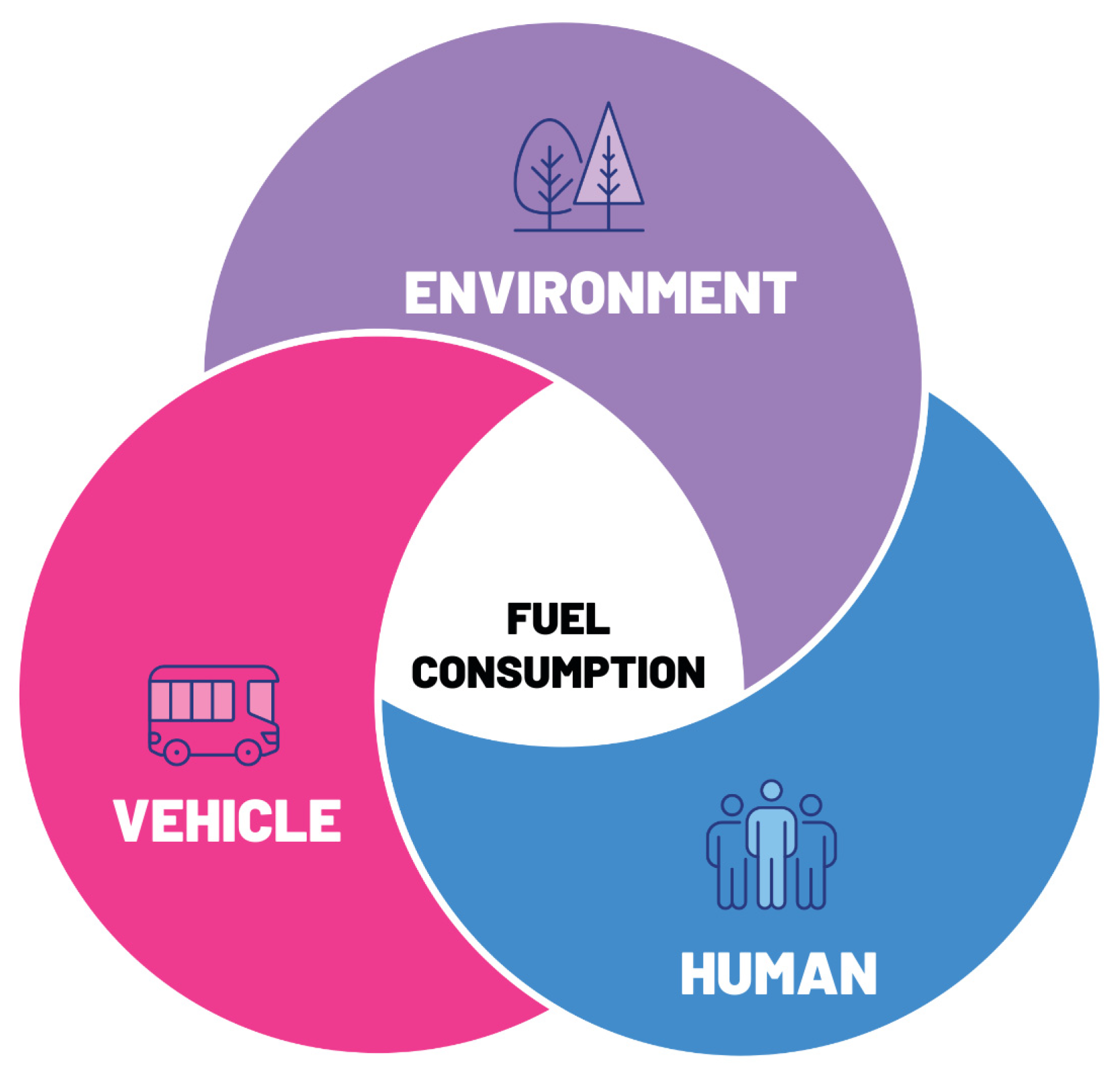
The fuel consumption assessment method proposed in this study is based on the practical observation that fuel use in heavy-duty machinery results from the interaction of three areas operating simultaneously. These include the operating environment, the technical characteristics of the vehicle and the human factor associated with the operator. In practice, these three domains form a single interacting system, and fuel consumption is the measurable outcome of their combined effect. This concept, frequently highlighted in operational studies of transport and mining machinery, is reflected in the Environment–Vehicle–Human diagram, where fuel consumption remains at the centre of the interaction.
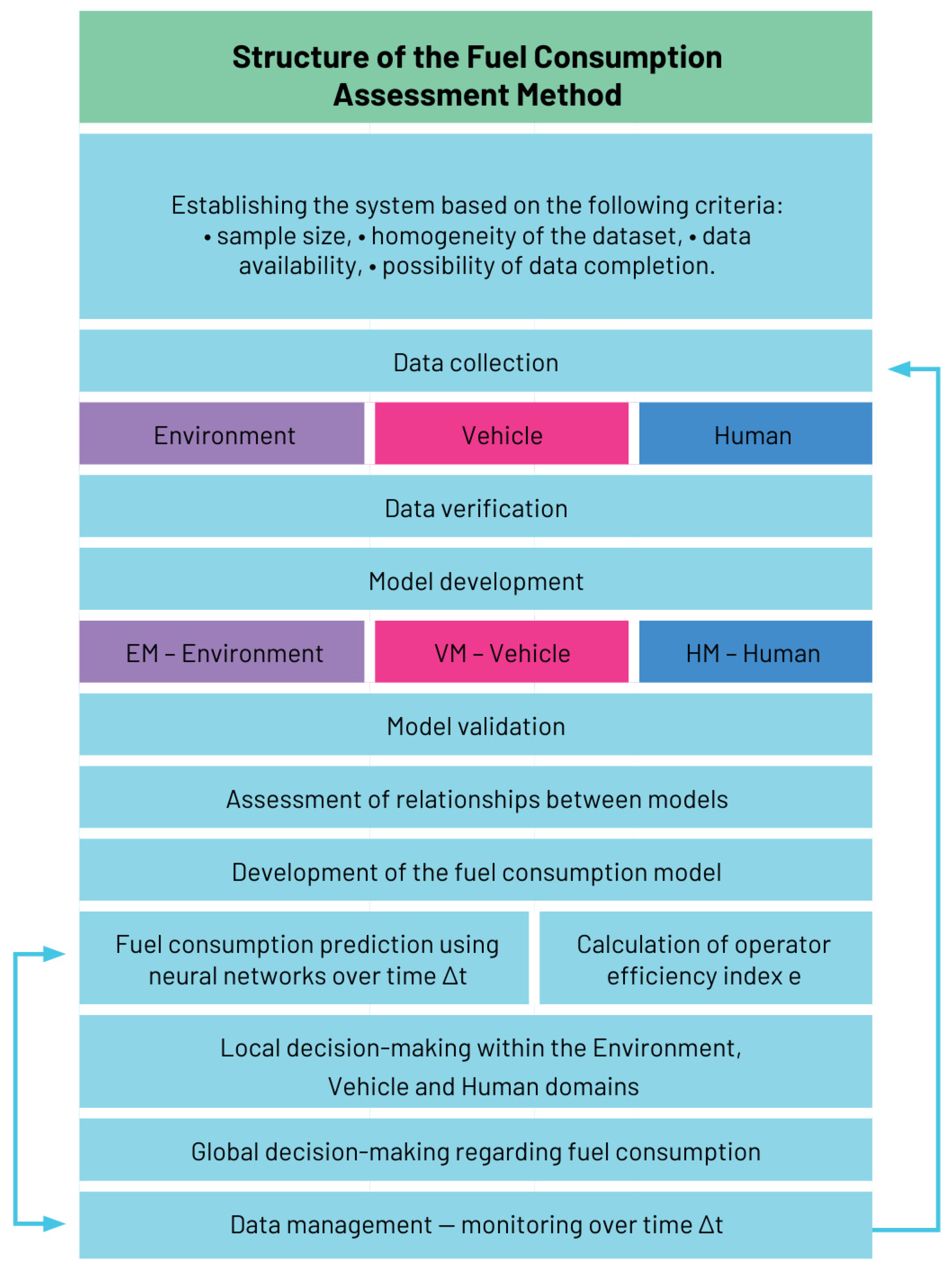
The development of the method followed a sequence that mirrors the logic of real data processing. At the beginning, it was necessary to define the boundaries of the system by specifying criteria such as dataset size, data homogeneity, availability and the possibility of completing missing records. Only after meeting these requirements was it possible to proceed with the main analytical stages: data collection, verification of raw signals, construction of individual models and validation of the selected variables. These stages correspond directly to the workflow shown in the methodological diagram and illustrate how raw operational data are transformed into a structured analytical model.
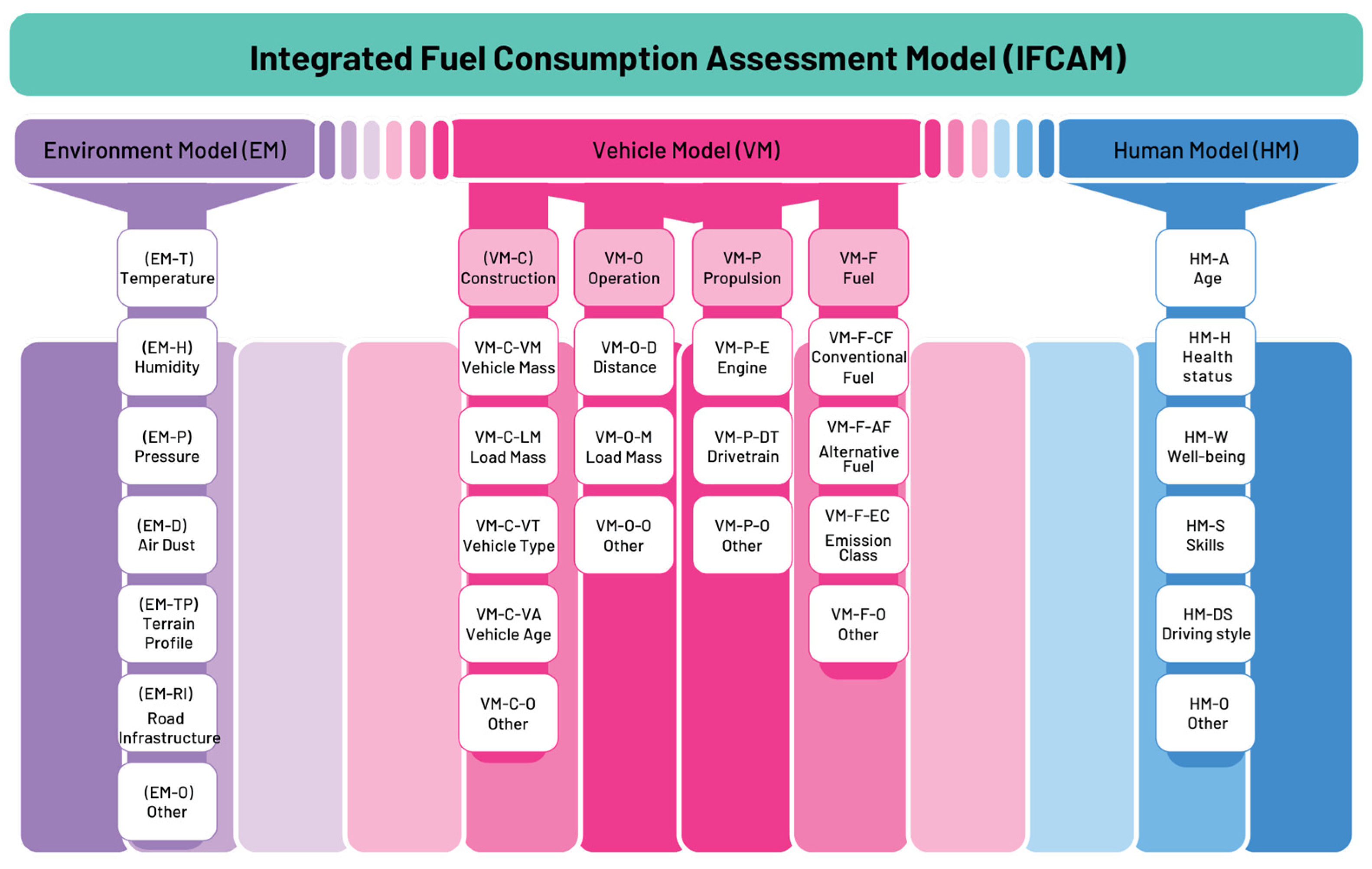
The central component of the method is the Integrated Fuel Consumption Assessment Model (IFCAM). This structure groups all relevant variables into three coherent areas: the Environment Model (EM), the Vehicle Model (VM) and the Human Model (HM). The EM includes parameters typical for underground and open-pit conditions, such as temperature, humidity, pressure, dust level, terrain profile or road infrastructure. The VM comprises construction-related factors, operating conditions, engine and drivetrain characteristics and the type of fuel used. The HM includes operator-related features such as age, health status, well-being, skills and driving style, which directly influence the energy demand of the machine.
A key feature of the IFCAM structure is the clear placement of each parameter within its functional category. This makes the model scalable and adaptable to other machine types, construction equipment and road transport fleets. Its modular architecture also allows for further extensions, for example by including new vehicle propulsion technologies or additional behavioural indicators.
In the final stage, the validated EM, VM and HM variables are integrated into the fuel consumption model, which becomes the basis for subsequent analytical and optimisation tasks. Although this paper does not discuss the operator efficiency index or neural network prediction modules, the method preserves the ability to incorporate these elements in separate studies.
Overall, the diagrams used in this section illustrate how the assessment method progresses from defining the operational system, through modelling the three core domains, to the final integration step that forms the IFCAM. Taken together, these components provide a transparent and consistent methodology for evaluating fuel consumption under real and continuously changing operating conditions.
3.1. Structure of the Integrated Fuel Consumption Assessment Model
The Integrated Fuel Consumption Assessment Model (IFCAM) is built on three fundamental components: the Environment Model, the Vehicle Model and the Human Model, as shown in
Figure 1. Each component groups variables that describe a separate area of influence on fuel consumption. The model can be applied to different types of machinery, including underground and surface mining equipment, construction machines, transport vehicles, agricultural machinery and specialised industrial vehicles. The mining case presented in this study serves only as an example of implementation.
3.1.1. Environment Model (EM)
The Environment Model groups external physical and infrastructural conditions in which the machine operates. These factors do not depend on the vehicle or the operator and describe the characteristics of the location in which the machine performs its tasks.
The EM includes the following variables:
EM-T—temperature: ambient temperature in the working area;
EM-H—humidity: relative air humidity;
EM-P—atmospheric pressure: pressure at the operating site (e.g., depth underground or altitude above sea level);
EM-D—dust level: concentration of airborne particulate matter;
EM-TP—terrain profile: geometry of the ground or roadway, including inclines and local variations;
EM-RI—road or ground infrastructure: surface type and condition;
EM-O—other environment-specific parameters: factors characteristic for a specific location.
The Environmental Model is expressed as:
3.1.2. Vehicle Model (VM)
The Vehicle Model describes the characteristics of the machine itself. It consists of four sub-models: Construction, Operation, Propulsion and Fuel. This structure allows the model to be used for different machine types and applications.
- 1.
Vehicle Construction Sub-Model (VM-C)
VM-C-VM—vehicle mass (empty): base mass of the machine;
VM-C-LM—load mass: mass of the transported material;
VM-C-VT—vehicle type: classification based on function and configuration;
VM-C-VA—vehicle age: age or hours of operation;
VM-C-O—other construction parameters.
- 2.
Vehicle Operation Sub-Model (VM-O)
VM-O-D—distance or operating cycle type;
VM-O-M—load-related operational mass;
VM-O-O—other operating variables.
- 3.
Vehicle Propulsion Sub-Model (VM-P)
VM-P-E—engine: main propulsion unit;
VM-P-DT—drivetrain: type of transmission system;
VM-P-O—other propulsion-related factors.
- 4.
Vehicle Fuel Sub-Model (VM-F)
VM-F-CF—conventional fuel: standard diesel or gasoline fuels;
VM-F-AF—alternative fuels: biodiesel, dual-fuel or hybrid mixtures;
VM-F-EC—emission class: emission category of the vehicle;
VM-F-O—other fuel-related parameters.
3.1.3. Human Model (HM)
The Human Model groups operator-related factors that can influence fuel consumption. These parameters describe the physical and behavioural characteristics of the driver.
The detailed structure of the Integrated Fuel Consumption Assessment Model is presented in
Figure 2.
3.1.4. Final Integrated Fuel Consumption Formula
The complete model is obtained by integrating the three domains:
The functional form does not require all variables to be present in every use-case. Empty variables are treated as non-active parameters, allowing the model to be applied in sectors where only a subset of EM, VM or HM inputs is available.
The method is based on the sequence of steps used in the processing of operational data: system definition, data acquisition, verification, model construction and analytical integration. The workflow illustrates how raw machine data are transformed into an analytical structure.
After defining the complete functional form of the fuel consumption model, the next step is to link the mathematical structure with the practical workflow used to develop and apply the Integrated Fuel Consumption Assessment Model. The sequence presented in
Figure 3 shows the full procedure, starting from system definition and ending with decision-making and long-term monitoring. Each stage corresponds directly to the steps required to transform raw operational data into a validated and transferable fuel consumption model.
The first block of the schematic refers to the system establishment stage, in which the operational context and analytical constraints are defined. This includes specifying the dataset size, its homogeneity, completeness and the feasibility of supplementing missing segments. These criteria ensure that all three domains—Environment, Vehicle and Human—are represented with sufficient resolution to construct stable statistical models.
The next stages—data collection and data verification—reflect the practical process of acquiring and preparing raw signals. Data verification includes identification and removal of corrupted records, detection of missing values, spikes and outliers, as well as the assessment of internal consistency between related parameters. At this point, each variable is assigned to its proper category within the EM, VM or HM domain, which ensures correct interpretation during model development.
Following verification, the individual domain models are developed. This stage includes statistical evaluation of each parameter, its preliminary correlation with specific fuel consumption and the construction of regression-based functional dependencies, consistent with the approach used in the doctoral research. Model validation follows, comprising tests of statistical significance of coefficients, analysis of residuals, assessment of model stability and the examination of multicollinearity. Variables that demonstrate instability or lack of statistical relevance are eliminated. The validated EM, VM and HM are then used to assess relationships between the domains and to identify dominant factors or interactions that influence fuel consumption.
The final part of the schematic shows the transition from model development to application. The validated variables are integrated into the full fuel consumption model, which can be used for several analytical purposes:
Short-term prediction, for example, by applying neural networks to forecast fuel consumption over a future time interval Δt;
Operator performance assessment based on the efficiency index e, used for comparative analysis between operators or shifts;
Local decision-making within a selected Environment, Vehicle or Human domain, allowing adjustments to operational practices or machine parameters;
Global decision-making, supporting fleet-level or organisational strategies aimed at reducing fuel consumption;
Long-term data management, enabling continuous monitoring of changes in the system and updating the model when new operational conditions occur.
The schematic therefore summarises not only the construction of IFCAM but also the entire procedure required for its practical implementation. Because each element of the workflow is independent and modular, the method can be applied across various sectors beyond mining, including construction machinery, agricultural equipment, municipal service vehicles and heavy road transport. The only requirement is that the available operational variables are assigned to the relevant EM, VM or HM categories. Once this condition is met, the same workflow can be followed to construct a complete and transferable fuel consumption model.
4. Study System and Data (Corrected and Validated)
The Integrated Fuel Consumption Assessment Model (IFCAM) was developed using long-term operational data from a large underground mining complex in Europe. The system comprises three underground mines with a combined annual ore production of approximately 30 million tonnes. Mining is carried out at depths of about 1000–1200 m, where the geothermal gradient reaches roughly 1 °C per 32 m of depth, resulting in high ambient temperatures in the working areas.
4.1. Environmental Conditions
The analysed mine operates in demanding thermal and atmospheric conditions typical for deep underground extraction. Daily measurements collected across more than ten production districts showed:
Dry-bulb temperature (EM-T): 33.7–37.0 °C;
Climate substitute temperature: 28.9–31.0 °C;
Relative humidity (EM-H): ≈90%;
Airflow velocity (EM-O): 0–2 m/s;
Dust concentration: high and stable;
Roadway inclination: ≤5°;
roadway dimensions:
- –
width ≥ 4.6 m;
- –
height typically 2–4 m, depending on ore thickness.
These values are consistent with the geothermal conditions of underground workings at depths above 800 m, where rock temperatures reach +35 to +46 °C, requiring the use of central cooling installations with cooling capacities above 15 MW.
The environmental characteristics listed above were used directly in the Environment Model (EM), as they represent the physical boundary conditions under which LHD perform repetitive loading–hauling–dumping cycles.
4.2. Vehicle Population and Machine Selection
The mining company operates a fleet of approximately 1200 heavy-duty vehicles, including trucks, loaders, drilling rigs and auxiliary machinery. Within the analysed mine, 507 machines operated underground.
For IFCAM validation, a homogeneous population of 45 loading machines (LHDs) was selected from a total of 123 loaders in the fleet. In addition, prior to selecting a single machine for high-frequency telemetry-based modelling, a representativeness check was conducted using monthly fuel consumption data for the entire analysed loader fleet operating in the investigated underground copper mine. A hypothesis was formulated that one representative loading machine can reflect the fuel consumption behaviour of the remaining units within the same class, and this assumption was statistically verified using the 2021 monthly dataset. The Friedman repeated-measures ANOVA indicated no statistically significant differences in fuel consumption across months for the analysed machines, supporting the use of one representative unit for detailed telemetry-based modelling. This group was chosen because:
All machines shared the same engine type and drivetrain configuration;
They performed the same type of work (short-distance loading and hauling);
They represented the highest annual fuel consumption within their category.
The annual fuel use of these 45 loaders exceeded 4.14 million dm3, making them the most fuel-intensive group on site.
Typical technical properties of the selected LHD class include:
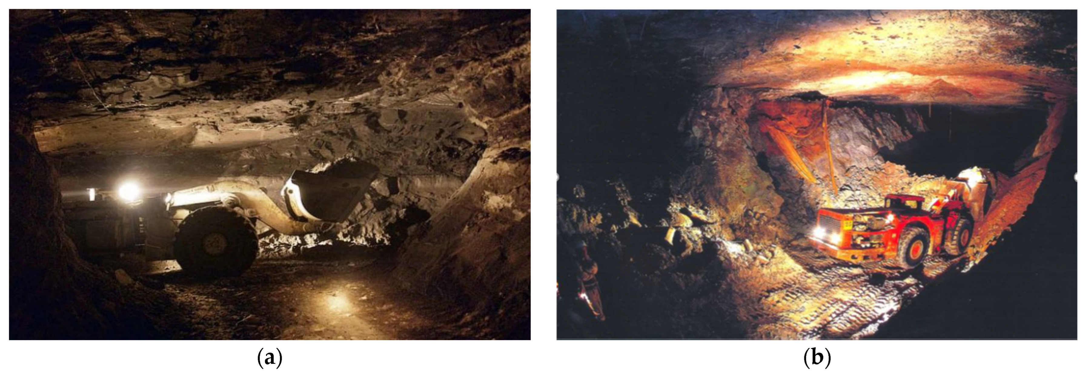
These characteristics correspond to the parameters included in the Vehicle Model (VM), particularly in construction-, operation- and propulsion-related components. To illustrate the operating conditions and the type of machinery included in the study, two representative photographs of underground loading equipment are shown below. The images in
Figure 4 document the typical working environment, roadway geometry, dust level and spatial limitations characteristic of the analysed system. They also reflect the conventional configuration of the LHD loader class selected for IFCAM validation.
4.3. Human-Related Factors
The dataset included 41 operators assigned to the selected LHD group. Each operator worked underground for approximately 6 h per shift in a four-shift system.
Although detailed demographic data (age, health records) were not available, all operators met the required medical and training criteria for work in deep underground conditions.
The only operator-related factor that could be reliably assessed was the driving style, represented in the data by:
Engine speed n [rpm];
Engine torque M [Nm];
Effective work time t [s];
Transported material mass per cycle m [t];
Instantaneous fuel use in [dm3/h].
These behavioural differences were included in the Human Model (HM). No unsupported numerical ranges describing fuel variability were added.
4.4. Monitoring System and Data Structure
All selected machines were equipped with an on-board diagnostic and monitoring system recording data with a frequency of 1 Hz. The system captured over 30 separate parameters, including:
Engine state variables;
Drivetrain load and temperatures;
Hydraulic system pressures and temperatures;
Payload measurements;
Selected environmental indicators.
This temporal structure allowed the IFCAM method to be applied consistently across machines performing repetitive tasks under similar boundary conditions.
In addition to raw monitoring signals, several derived quantities were calculated for the purpose of fuel consumption assessment. Engine speed n [rpm] and engine torque T [Nm] were obtained directly from the CAN/OBD interface, while instantaneous fuel flow was expressed as hourly fuel consumption (HFC). Based on these measurements, the specific fuel consumption (SFC) was calculated as the ratio of fuel mass flow to effective engine power. The engine power was computed from the measured torque and rotational speed using standard mechanical relationships. All variables were recorded or derived at a temporal resolution of 1 s, allowing SFC to be evaluated under transient, real-world operating conditions. It should be noted that the reported SFC represents an operational indicator and does not correspond to laboratory brake-specific fuel consumption determined under steady-state dynamometer testing.
4.5. Data Pre-Processing
Data pre-processing followed a structured multi-stage verification procedure:
3–7% of records were removed due to missing data, corrupted values or unrealistic spikes;
Only short gaps of ≤2–3 s were interpolated;
After verification, 93–97% of all signals remained valid;
All four phases of the operational cycle (loading, loaded haul, dumping, return) were automatically identified and aligned.
This ensured that the dataset fulfilled the requirements of IFCAM regarding completeness, homogeneity and repeatability. This ensured that the dataset fulfilled the requirements of IFCAM regarding completeness, homogeneity and repeatability. The key characteristics of the validated dataset are summarised in
Table 1.
5. Results and Analysis
The Integrated Fuel Consumption Assessment Model (IFCAM) was applied to the operational dataset obtained from the underground mining system discussed in
Section 4. The purpose of this part of the study is to examine how the three components of the model—environment, vehicle and operator—shape fuel consumption during real repetitive loading–haul–dump cycles.
In this article IFCAM is demonstrated on one industrial case: an underground copper mine in Europe. The site was selected because it provides continuous work cycles, stable boundary conditions and long-term monitoring data. These features make it suitable for validating the method, even though IFCAM itself is not limited to mining applications and can be transferred to other heavy-duty vehicles.
To ensure a consistent analytical sample, the study focused on one machine class operated in large numbers at the site. Out of 45 LHD loaders equipped with the same engine and drivetrain configuration, 38 units met the completeness criteria and were included in the analysis. This allowed the dataset to remain homogeneous while still providing sufficient statistical diversity for model validation. The same selection logic can be applied to other groups of machines when IFCAM is used in different sectors.
The sections that follow present the results obtained for the environmental, vehicle and operator domains, as well as the combined relationships between these factors. All results are based solely on the measured 1 Hz data without introducing external assumptions.
5.1. Environmental Conditions and Their Impact on Fuel Use
Validation of the Environmental Model (EM) focused on identifying which environmental parameters exhibited sufficient variability and statistical relevance to justify their inclusion in the final IFCAM structure. Long-term operational measurements showed that most environmental variables characterising the analysed system remained effectively constant during machine operation. Relative humidity (≈90%), dust concentration (high and stable), roadway inclination (≤5°) and airflow velocity (0–2 m/s) did not demonstrate meaningful variability and were therefore excluded from the regression analysis. These parameters define the boundary conditions of the operating environment and form part of the structural context of the model, but they do not explain differences in fuel consumption between machines.
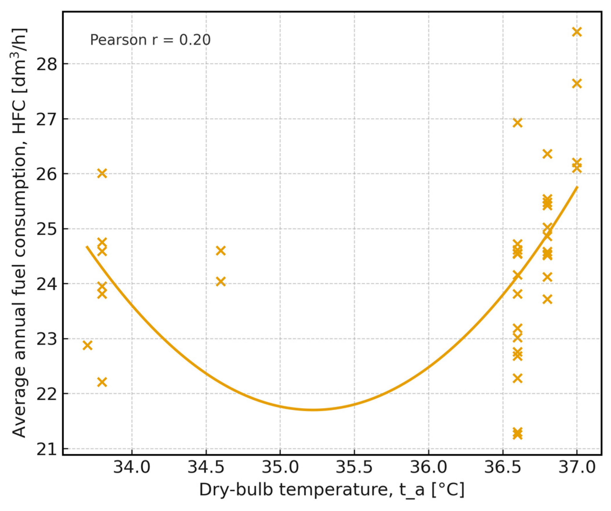
Among the environmental variables considered, dry-bulb temperature (t_a) was the only parameter that varied sufficiently within the observed range (33.7–37.0 °C) to allow its statistical assessment. This enabled a focused validation consistent with the variable-selection procedure applied throughout the IFCAM framework. The analysis comprised exploratory statistics, correlation testing and trend visualisation to examine the association between temperature and hourly fuel consumption.
The results indicate a statistically detectable but moderate relationship between ambient temperature and fuel consumption. As illustrated in
Figure 5, the distribution of data points suggests a non-uniform tendency across the observed temperature range, reflected by a Pearson correlation coefficient of r = 0.20. The fitted polynomial curve is used solely as an exploratory visual indicator of an aggregated trend and does not imply interpolation or a deterministic functional relationship, particularly in temperature intervals with limited data availability. Consequently, the interpretation is limited to correlation-based assessment rather than causal inference.
Although temperature accounts for a smaller share of fuel consumption variability compared with factors represented in the Vehicle Model (VM) and Human Model (HM), its inclusion contributed to improved overall model stability and reduced residual error. It should be emphasised that the environmental conditions analysed in this study serve as an application example, demonstrating how IFCAM identifies and validates relevant environmental predictors. The same methodological procedure can be applied to construction, transport or agricultural machinery, where environmental parameters may exhibit wider variability and thus exert a more pronounced influence on fuel consumption.
5.2. Vehicle Model (VM) Validation
The Vehicle Model (VM) was initially structured into four conceptual groups: (i) vehicle construction, (ii) operating profile, (iii) propulsion system, and (iv) fuel type. In the present case study, all analysed machines belonged to the same class of underground wheel loaders, equipped with the same diesel engine, identical drivetrain layout and supplied exclusively with standard diesel fuel. As a result, several construction—and fuel-related variables remained constant across the fleet and could not be used as explanatory predictors in the regression layer of IFCAM. Their role was structural: they defined the machine class and boundary conditions of the analysed system.
A full dataset was available for 38 machines of the same model, each of which operated for a complete year without long shutdowns. For every machine, monthly and annual fuel consumption and operating hours were recorded, allowing the calculation of average hourly fuel consumption HFC [dm3/h] at both monthly and annual levels. In 2021 the highest monthly average HFC was observed in December (25.42 dm3/h), while the lowest was recorded in May (23.21 dm3/h). The overall mean for the fleet was 24.37 dm3/h. At the machine level, the most fuel-intensive unit reached an annual average of 28.58 dm3/h, whereas the lowest value was 21.25 dm3/h.
5.2.1. Machine Age and Fuel Consumption
Machine age (expressed in decimal years since commissioning) was evaluated as a potential contextual descriptor within the Vehicle Model. The normality of its distribution was examined using several tests, including Kolmogorov–Smirnov, Lilliefors, Shapiro–Wilk and D’Agostino–Pearson. Although the Kolmogorov–Smirnov test suggested approximate normality (p = 0.288), the more sensitive tests for small samples (n = 38) indicated that the age distribution deviated significantly from normality (Lilliefors p = 0.021, Shapiro–Wilk p = 0.036, D’Agostino–Pearson p = 0.023). This justified the use of non-parametric correlation methods.
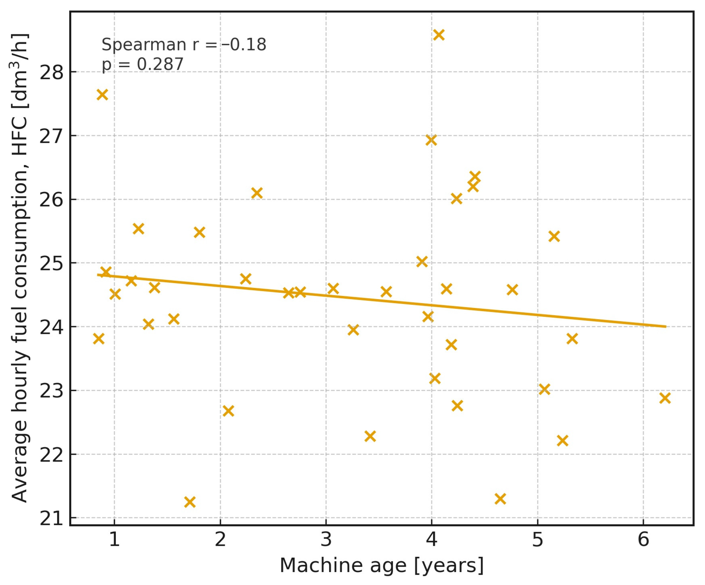
The monotonic relationship between machine age and average operational fuel use, expressed as mean hourly fuel consumption (HFC), was therefore analysed using Spearman’s rank correlation. The resulting coefficient was r = −0.174 with
p = 0.295 (95% CI: −0.48 to 0.16), indicating no statistically significant association between machine age and average hourly fuel consumption. The corresponding scatter plot (
Figure 6) shows substantial dispersion of data points without a consistent trend, supporting this conclusion. Consequently, machine age is not interpreted as a direct explanatory variable of engine fuel efficiency, but rather as a contextual characteristic reflecting fleet composition and operational assignment.
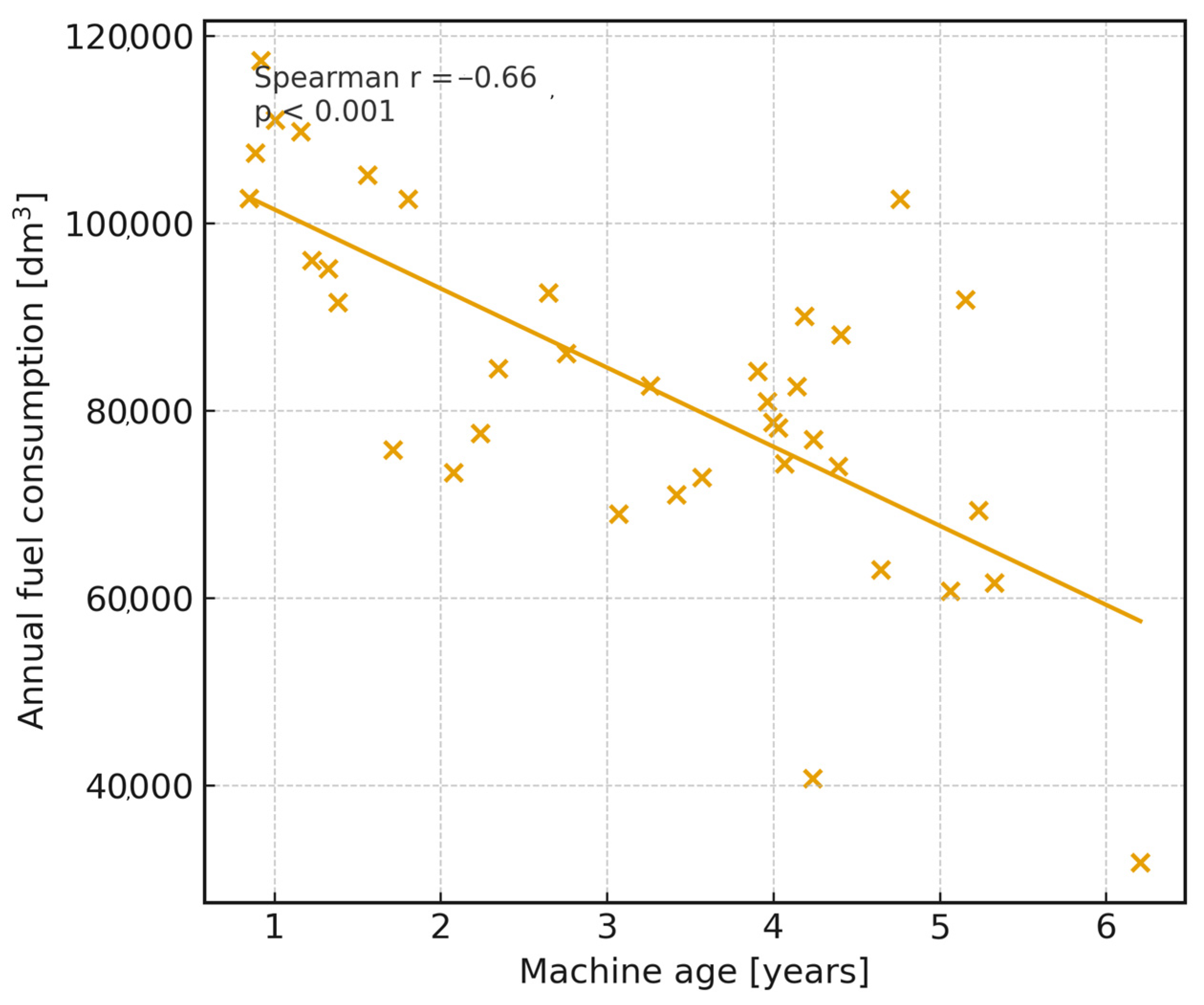
In the second step, the relationship between machine age and total annual fuel consumption, defined as the sum of fuel dispensed during 2021, was evaluated. In this case, a strong and statistically significant negative correlation was observed, with Spearman r = −0.686 (95% CI: −0.83 to −0.46, p = 0.000002). Older machines were associated with lower total annual fuel consumption, which reflects reduced utilisation and task allocation patterns rather than improved energy efficiency. This result is important for IFCAM, as machine age acts as an indicator of fleet-level utilisation, while it does not explain differences in specific hourly fuel consumption between machines.
5.2.2. Fleet-Level Consistency of Hourly Fuel Consumption
A key methodological question for IFCAM was whether a single representative machine could be used for detailed telemetric analyses instead of processing complete high-frequency data from all 38 units. To address this issue, statistical tests were carried out to verify the consistency of hourly fuel consumption (HFC) at fleet level.
A non-parametric repeated-measures ANOVA (Friedman test) was applied to monthly HFC values for all machines operating in 2021. The test compared hourly fuel consumption across the annual operating period for the analysed fleet. The Friedman statistic was T
1 = 19.25 with
p = 0.0568, slightly above the conventional 0.05 significance threshold. This result indicates that no statistically significant differences in hourly fuel consumption were detected across the analysed period, supporting the assumption of temporal consistency at fleet level. The dispersion of values observed in
Figure 7 reflects operational variability rather than systematic temporal effects.
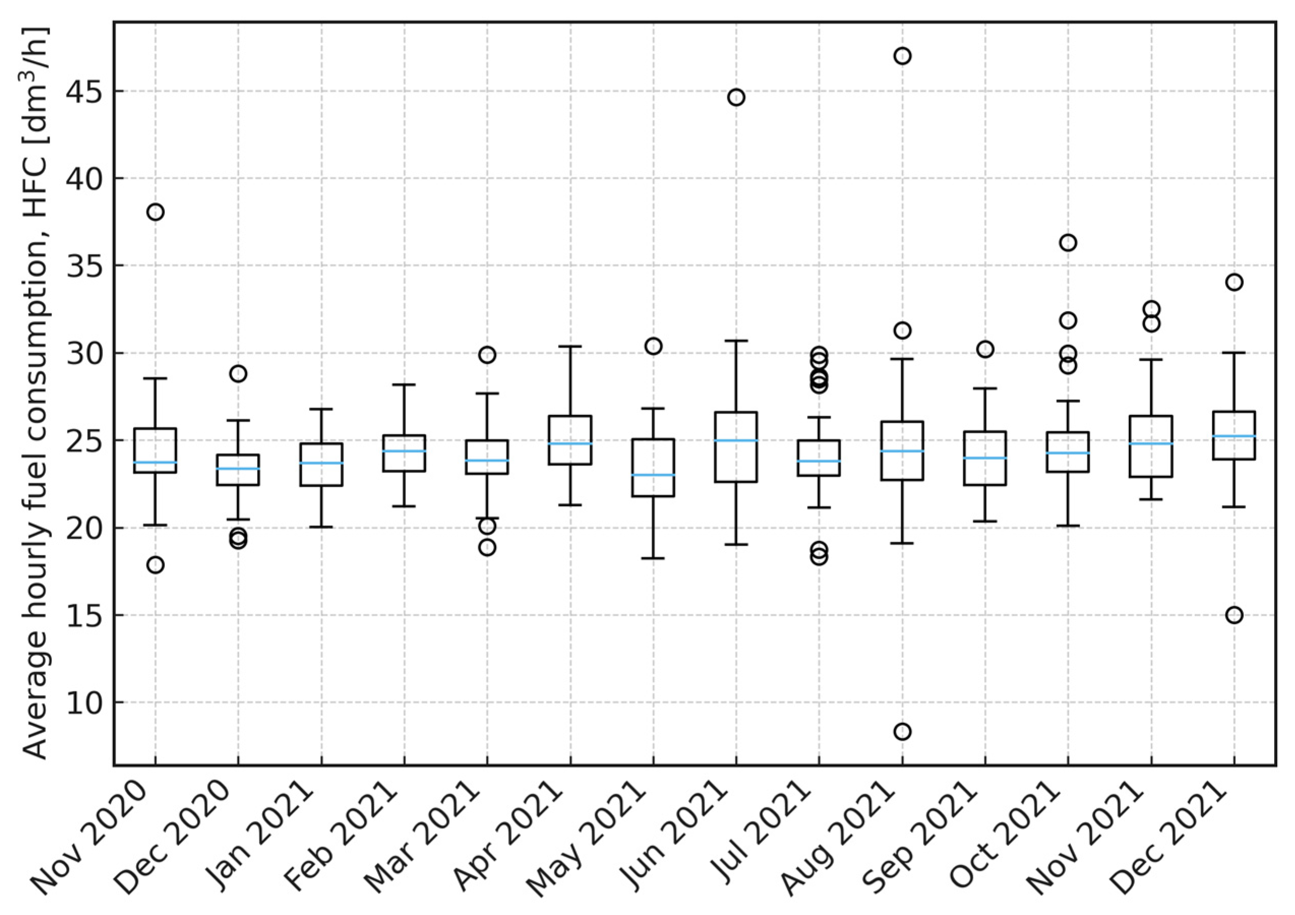
Figure 8 presents the distribution of hourly fuel consumption (HFC) for all 38 machines across fourteen consecutive months (November 2020–December 2021). The results show that HFC remains within a narrow and stable range of approximately 23–26 dm
3/h throughout the entire observation period. Median values for all months are closely aligned, and interquartile ranges are relatively uniform, indicating comparable loading conditions and similar operational profiles over time.
A small number of outliers correspond to isolated periods of higher engine load but do not alter the overall distribution pattern. Importantly, no visible month-to-month shift in central tendency or dispersion is observed. This visual inspection is consistent with the Friedman test, which did not identify statistically significant differences in HFC between months.
The stability of monthly HFC distributions confirms that the fleet operates under consistent duty cycles and supports the methodological assumption that a single unit can be treated as representative for high-resolution telemetric analyses within IFCAM.
Next, the Kendall’s coefficient of concordance W was used to assess the agreement of HFC values between machines across months. In this formulation, each machine acted as a “judge” assigning ranks to months (or conversely, each month acted as a judge ranking machines). The resulting coefficient was W = 0.385, with an associated chi-square statistic of 170.82 and p < 0.000001. The corresponding average pairwise Spearman correlation between machines was 0.329. These values indicate a moderate but statistically highly significant level of agreement in hourly fuel consumption across the fleet.
Together, the Friedman and Kendall tests support the hypothesis that the machines exhibit statistically consistent hourly fuel consumption behaviour over time. On this basis, the following working hypothesis was accepted:
H1: A single machine of the analysed type can be treated as representative of the entire fleet with respect to hourly fuel consumption.
This conclusion is essential for the design of IFCAM. It justifies the reduction in data volume by focusing detailed, high-frequency analyses (e.g., engine speed, torque, instantaneous fuel rate, bucket load) on one carefully monitored reference machine, while fleet-level effects remain captured by aggregated VM parameters (age, utilisation and HFC distributions).
5.2.3. Implications for the Vehicle Model in IFCAM
In summary, VM validation for this case study showed that:
Construction-related and fuel-related parameters remained constant and therefore define the machine class rather than explain variability in fuel consumption.
Machine age does not significantly influence average hourly fuel consumption, but it is strongly and inversely correlated with annual fuel use due to reduced utilisation of older machines.
Hourly fuel consumption patterns are statistically consistent across the 38 machines, which validates the use of a single representative machine for in-depth telemetric analysis within IFCAM.
As a result, the Vehicle Model in this implementation of IFCAM incorporates age and utilisation measures at fleet level, while load- and engine-related variables derived from telemetric data are further analysed within the Human Model (HM), where they are attributed to operator behaviour rather than to the vehicle itself.
5.3. Validation of the Human Model (HM)
The Human Model (HM) component of the fuel-consumption framework was validated using high-resolution telemetric data obtained from one load–haul–dump (LHD) machine operated over 18 days by 41 operators. The objective of this analysis was to isolate and quantify the behavioural contribution to fuel consumption under stable environmental, organisational and vehicle-related conditions. Since individual-level demographic or physiological data (age, training level, fatigue, health status) were not available, operator influence was inferred exclusively from behavioural patterns represented in engine-related variables. This approach is consistent with contemporary research demonstrating that behavioural signatures—rather than self-reported characteristics—are often the most reliable proxy for driver-induced variability in energy demand.
5.3.1. Data Characteristics and Behavioural Indicators
The telemetric system recorded engine speed n [rpm], engine torque T [Nm], instantaneous fuel rate, specific fuel consumption SFC [g/kWh] and, where available, bucket load mass m [t]. Across several hundred thousand observations sampled at 1 Hz:
Mean engine speed ≈ 1539 rpm;
Mean torque ≈ 483 Nm;
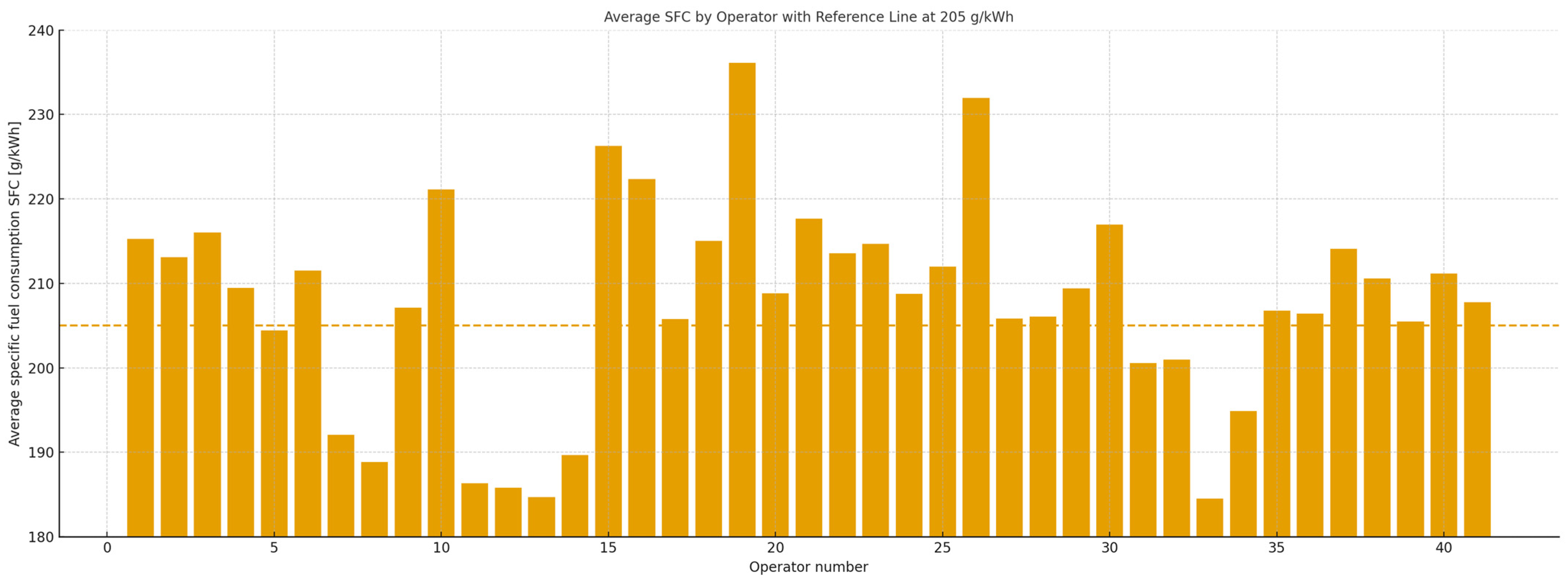
Mean SFC ≈ 208 g/kWh, close to the nominal 205 g/kWh reference;
Operator-level SFC ranged widely between ≈184 g/kWh and ≈236 g/kWh.
This wide dispersion occurred despite all operators using the same machine, in the same environment, and performing the same task—strongly suggesting a behavioural origin rather than mechanical or contextual causes. Missing data in bucket-load measurements indicated inconsistencies in the measurement system; however, where mass data were available, distribution patterns provided additional behavioural context. Normality tests (Kolmogorov–Smirnov, Lilliefors) confirmed non-normal distributions for all variables (p < 0.01), necessitating non-parametric statistical methods.
5.3.2. Operating-Field Analysis
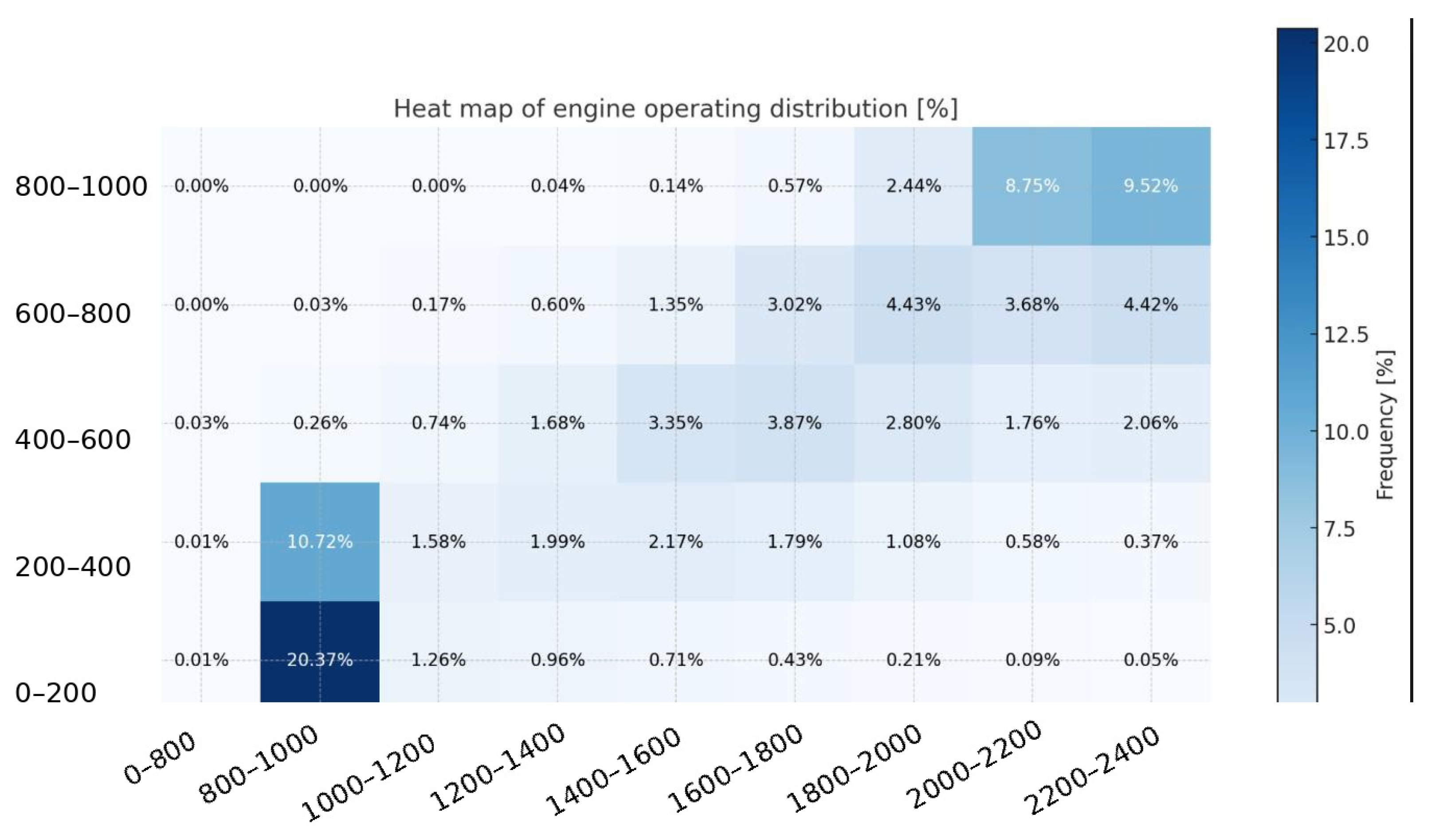
To evaluate how operators utilise the available powertrain, engine operating points were mapped into the torque–speed (
n–T) plane and discretised into 45 subregions representing distinct operating states, ranging from idle and low-load conditions to near-maximum power demand. The distribution of operating points is shown in
Figure 9 in the form of a heat map, which expresses the relative frequency of occurrence of each operating state based on 1 Hz telemetry data.
Based on this distribution, operating points were classified into predefined specific fuel consumption (SFC) ranges in order to quantify the share of operating time spent in different efficiency regions. This analysis revealed pronounced behavioural clustering. Approximately 3% of total operating time was spent in the most fuel-efficient SFC region (≈180–200 g/kWh), while an additional ~9% corresponded to an extended efficiency range. In contrast, approximately 97% of operating time was associated with operating states in which SFC exceeded 200 g/kWh. These values represent empirical time shares derived from the classification of all recorded operating points and do not constitute predefined or assumed performance categories.
Two dominant operating regimes can be identified. First, a large concentration of points occurs at low engine speeds (≈800–1000 rpm) and low torque levels (<200 Nm), corresponding to idle and low-load operation. Although mechanical load in this region is limited, fuel is consumed with minimal productive output, resulting in unfavourable energy efficiency. Second, a distinct concentration of operating points appears at high engine speeds (>1600 rpm) and high torque levels approaching machine limits (≈850–1000 Nm). In this region, previously identified SFC values increase markedly due to enriched fuel dosing, elevated thermal loads and reduced combustion efficiency under near-maximum power demand.
Taken together, these results indicate that operators spend only a limited fraction of total operating time within the thermodynamically favourable efficiency region, while the majority of operation occurs either at low-load conditions or at high-load, high-speed states associated with elevated specific fuel consumption. This finding highlights the dominant role of operator behaviour in shaping real-world fuel consumption patterns and provides a quantitative basis for efficiency-oriented operational assessment within the IFCAM framework.
5.3.3. Efficient vs. Inefficient Operators: Behavioural Signatures
To isolate behavioural effects, operators were ranked by mean SFC, considering only those with ≥2.5 h of recorded work to ensure representativeness, shown on
Figure 10.
Efficient operators (SFC ≈ 200–201 g/kWh)
These operators exhibited:
59–75% of operating time in low- and mid-speed regions (800–1600 rpm);
Minimal sustained operation at high torque/speed;
Smooth, evenly distributed operating-point fields.
Their rpm–SFC curves showed a predictable pattern: SFC rises gradually with rpm up to ~1500 rpm, then stabilises around ~210 g/kWh—typical of conservative, controlled driving.
Inefficient operators (SFC ≈ 232–236 g/kWh)
In contrast, inefficient operators:
Spent 52–58% of time above 1600 rpm;
Showed pronounced clustering near the machine’s upper speed and torque limits;
Displayed distinct “bands” of high SFC (220–240 g/kWh) across large rpm intervals.
Their behaviour indicates persistent operation in high-load states, consistent with over-aggressive throttle application, insufficient modulation and prolonged peak-power usage. These behavioural archetypes correspond well with human-factor findings in heavy-vehicle operations: operators with smoother pedal modulation and load anticipation consistently achieve lower energy consumption.
Spearman correlation analysis conducted for the full dataset revealed the following relationships:
Engine speed and torque were highly positively correlated (r ≈ 0.78), which reflects the mechanical interaction between throttle application and engine-load generation;
Both variables showed a moderate positive correlation with specific fuel consumption (r ≈ 0.47–0.49), indicating that increases in speed and load lead to higher fuel demand;
Bucket payload exhibited only a weak, although statistically significant, correlation with fuel consumption, suggesting that the presence of load contributes to fuel use, but its influence is secondary relative to operator-induced changes in speed and torque.
To verify whether bucket load introduced meaningful differentiation, the dataset was divided into two subsets:
A Mann–Whitney U test confirmed statistically significant differences in fuel-consumption distributions between these groups (p < 0.05); however, the magnitude of the effect was small. This result supports the interpretation that for this machine type, fuel consumption is predominantly driven by operator behaviour rather than by variations in transported mass.
5.3.4. Implications for the Human Model and Energy Efficiency
Prior to inclusion in the Human Model, all behavioural indicators were subjected to statistical significance testing using non-parametric methods. Only variables demonstrating statistically significant relationships with specific fuel consumption were retained as explanatory inputs in the IFCAM framework.
The validation outcomes clearly indicate that operator behaviour constitutes the dominant source of variability in fuel consumption when environmental and machine-level conditions remain stable. This leads to several practical insights:
Differences attributable to individual operators exceed those originating from machine tolerances. Under identical conditions, variations in SFC between operators reached 28–30%.
Operators rarely utilise the most efficient operating region; time spent in these favourable ranges amounted to only approximately 3–9% of total operating time. Consequently, behavioural modification and operator training represent an effective path toward energy-efficiency improvement.
Metrics derived from operating-field distributions show strong discriminative capability. Heatmaps and statistical profiles provide identifiable patterns characteristic of each operator, enabling targeted feedback, personalised instruction, or performance-based incentives.
Fuel consumption can be modelled using behavioural metrics alone. The joint distribution of engine speed, torque, payload mass and SFC sufficiently captures differences in driving style and supports prediction within the Human Model.
Accordingly, the Human Model incorporates:
Engine speed n [rpm];
Engine torque T [Nm];
Bucket load m [t];
Specific fuel consumption (SFC); and
Distribution-based indicators quantifying time spent inside and outside efficient operating regions. These variables form the behavioural input layer of the IFCAM framework, enabling accurate prediction, energy-efficiency optimisation and systematic evaluation of operator performance.
6. Development of the Fuel-Consumption Model
Based on the analyses performed for the environment, vehicle and operator-related variables, three operational parameters were identified as relevant predictors of specific fuel consumption (SFC): engine speed , torque and payload mass . Since mass registration was not active for all operators, zero readings could not be interpreted unequivocally either as actual zero payload or as missing data. For that reason, zero values originating from inactive measurement were treated as missing observations and removed from the regression dataset.
A multiple linear regression was then developed using only the records where the payload value was valid. The resulting model was statistically significant (F = 7363.3;
p < 0.0001), and all independent variables contributed significantly to explaining variation in SFC. The obtained regression equation was:
The coefficient of determination was , which is appropriate when considering the nature of the data, characterised by transient operating states and strong operator-driven variability. For in situ production conditions, involving non-stationary cycles and behavioural influence, such a level of explained variance is consistent with real operating variability. The standard estimation error was approximately 27 g/kWh, which corresponds to typical fluctuations observed during underground loading cycles.
Residual inspection confirmed appropriate reproduction of average trends, with predicted values aligning along the trajectory of the measured points. Thus, the regression model provides a referential analytical form describing average SFC behaviour as a function of , and , and served as a baseline model for subsequent nonlinear prediction.
7. Nonlinear Prediction of SFC Using a Neural Network
To capture nonlinear relationships between the operational variables and instantaneous fuel consumption, a predictive model in the form of an artificial neural network was developed. The model was trained using approx. 2 million recorded observations from 2.5 weeks of operation of a single loader used by 41 operators.
A multilayer perceptron (MLP) network with the architecture 3-8-1 was implemented, comprising three inputs (n, T, m), one hidden layer with eight neurons and one output representing SFC. The dataset was divided chronologically into training (70%), testing (15%) and validation (15%) subsets in order to preserve temporal structure and avoid temporal leakage. Random sampling was deliberately avoided due to the time-dependent nature of operational data. The hidden layer used the tanh activation function, while the output neuron employed a logistic activation function.
The model achieved high correlation coefficients between observed and predicted values:
training phase: 0.9645
testing phase: 0.9647
validation phase: 0.9648
The uniformity of these values confirms proper generalisation and the absence of over-fitting. The network provided accurate predictions for both individual operating states and time sequences of machine use. The strongest influence on the output response was linked to engine speed and torque, whereas payload mass improved estimation accuracy for phases associated with real loading conditions.
The model was exported in PMML format, enabling direct integration with monitoring systems processing online CAN data. This allows real-time estimation of fuel-consumption behaviour, quantification of operator-dependent efficiency and operational cost evaluation. In summary, the linear regression offers an interpretable analytical relationship describing the average influence of operational variables, whereas the neural network effectively reflects dynamic, instantaneous and operator-dependent variability of fuel demand. Together, these approaches constitute a comprehensive modelling framework suitable for energy-efficiency assessment under real exploitation conditions.
8. Discussion
The presented research introduces a structured method for assessing fuel consumption of heavy-duty machines, based on the combined influence of environmental, vehicle and human-related factors. Using long-duration operational data from a full working cycle of an underground loader, the developed approach enabled separation of effects that remain inseparable under conventional reporting based only on averaged fuel indicators. This allowed for quantitative identification of the magnitude of machine-induced variability and operator-induced variability, with direct implications for operational optimisation. Although environmental parameters are traditionally considered a significant determinant of fuel usage, the collected dataset demonstrated that their influence was minimal under stable working conditions. Ambient temperature and humidity remained nearly constant over the monitoring period, eliminating their confounding effect on the model. This confirms that environmental factors in industrial mining systems, once stabilised, do not introduce systematic distortions in fuel demand, which justified their exclusion from predictive modelling. Machine-related parameters exhibited predictable but limited explanatory potential. Engine rotational speed and torque jointly accounted for approximately one-quarter to one-third of variance in specific fuel consumption. This aligns with general combustion characteristics of high-displacement diesel engines—fuel demand grows with torque and engine speed, but only a portion of this trend remains observable under real-operation duty cycles dominated by transient loading. The regression model, although statistically significant, displayed a moderate goodness-of-fit. This result is methodological rather than limiting; it demonstrates that consumption cannot be explained solely from engine thermodynamics and momentary load, despite correct physical directionality of the coefficients. The most pronounced finding arises from the human factor. Operator behaviour explained variability exceeding the mechanical effect, even though the machine operated in nominally identical working cycles. The proportion of time spent in load-efficient regions, modulation of throttle at onset of excavation, and stabilisation of torque during acceleration phases were key differentiators. Segmentation of operators based on measurable indicators resulted in differences in fuel consumption exceeding 25–30%, with no differences attributable to vehicle condition or external conditions. This confirms that behavioural patterns, even those not perceived consciously by operators, directly shift operating points into less efficient combustion zones. The load parameter, representing mass carried on the bucket, proved weakly correlated with consumption when considered alone. However, its significance emerged not as a physical effect, but as a structural differentiator that separated correctly measured cycles from incomplete loading sequences. The statistical test comparing SFC distributions showed significance, yet effect sizes remained low, again reinforcing that correct interpretation of load serves primarily as a qualifier of operational completeness rather than a causal driver.
Finally, the application of neural modelling verified the suitability of the selected predictors. Although linear regression identified directional significance of speed, torque and load, the neural networks captured the non-linear interactions that arise in actual machine duty cycles. A multilayer perceptron trained on the same dataset achieved high agreement between predicted and observed values, confirming that these selected indicators form a sufficient feature space for operational prediction. This coherence between physical interpretability (regression) and predictive adequacy (MLP) validates the methodological structure established in this work.
The empirical validation and parameter significance are reported for the investigated operational system—an underground copper mine. However, IFCAM is formulated as a general methodological procedure (data integration → statistical verification → model validation) that can be re-applied in other systems once system-specific data are available.
Collectively, the results confirm that a combined modelling approach—integrating machine state and operator profiles—provides a reliable basis for assessment and prediction of fuel consumption in heavy-duty operational environments.
Although the empirical validation presented in this study is based on underground mining machinery, the proposed IFCAM framework is formulated as a general fuel consumption assessment methodology and is not limited to a specific vehicle category or operating sector. The framework is applicable to a wide range of systems, including passenger cars, heavy-duty road vehicles, construction equipment and mining machinery. Depending on the application, the relative importance of environmental, vehicle-related and human-related factors may vary; however, the same methodological procedure of comprehensive data integration, statistical significance testing and model validation can be consistently applied without modification of the core framework.
Prediction Accuracy Comparison and Statistical Validation
To quantitatively assess the predictive performance of the proposed integrated framework, its accuracy was compared with a conventional baseline based on multiple linear regression (MLR). Both models were evaluated using identical input variables and the same dataset. The neural model corresponds to the multilayer perceptron (MLP 3-8-1) developed in the research and reproduced in this study using the original PMML specification, ensuring full consistency of network structure, normalisation procedures and learned parameters.
To avoid temporal leakage, the dataset was divided chronologically into training (70%), testing (15%) and validation (15%) subsets. Prediction accuracy was evaluated exclusively on the test subset, which was not used during model training. Model performance was quantified using the mean absolute error (MAE) and the root mean squared error (RMSE).
The baseline MLR model achieved an MAE of 20.45 g/kWh and an RMSE of 39.93 g/kWh. In contrast, the neural model achieved an MAE of 18.51 g/kWh and an RMSE of 37.34 g/kWh, indicating lower prediction errors for the nonlinear approach under identical data conditions.
To verify the statistical significance of the observed improvement, a paired t-test was conducted on the absolute prediction errors obtained for each observation in the test dataset. The analysis confirmed that the reduction in prediction error achieved by the neural model is statistically significant (p < 0.05). The mean reduction in absolute error relative to the baseline regression model amounted to approximately 1.9 g/kWh.
The results demonstrate that the proposed integrated modelling approach provides a measurable and statistically significant improvement over conventional regression-based methods while operating on the same set of input variables and data. This confirms the effectiveness of incorporating nonlinear relationships within a unified modelling framework for fuel consumption assessment.
9. Conclusions
This work proposed and validated a method for fuel consumption assessment in heavy-duty machinery by integrating environmental, vehicle and human components into a unified analytical framework. Based on long-term operational data collected from actual mining loaders, the following conclusions were established:
Environmental influence on consumption is negligible under stable site conditions.
Ambient parameters, despite being theoretically relevant, contributed no measurable variability and can be excluded from predictive models when working conditions do not vary.
Vehicle-related parameters retain clear physical relevance but moderate predictive strength.
Engine speed, torque and transported mass showed statistically significant correlations with fuel consumption, forming the basis for analytical modelling.
Operator behaviour is the dominant source of variability in real industrial operation.
Differences in throttle modulation, machine acceleration and load-handling approach resulted in consumption differences exceeding 25%, despite identical equipment and environment.
Linear regression provides interpretable, statistically correct relationships, but captures only part of real interactions.
The model correctly indicated the directionality of influence and quantified average consumption levels but remained limited by the inherent non-linearity of duty cycles.
Neural modelling enables accurate prediction using the same explanatory variables.
The MLP structure achieved high predictive agreement with observed data, confirming operational sufficiency of the selected input set and validating integration of human-behavioural characteristics.
The proposed method constitutes an applicable decision-support tool.
It allows classification of operator efficiency, assessment of machine usage patterns and prediction of future consumption, forming a basis for cost-reduction strategies, training interventions and operational scheduling.
In summary, the developed method provides both interpretability and predictive capability, allowing fuel consumption to be assessed not only retrospectively, but also controllably and proactively. The results provide a foundation for implementation in fleet monitoring systems, integration into telematic platforms, and development of behavioural efficiency indices supporting training and incentive programmes in heavy-industry applications.
