Abstract
To address the problem that transformer inrush currents under no-load and energization conditions can easily trigger misoperations of differential protection, this paper proposes a multi-feature identification method for transformer inrush current based on adaptive variational mode decomposition. Traditional methods typically rely on fixed physical features or single criteria, making them sensitive to operating condition variations and prone to misclassification or missed detection under complex disturbances, with limited generalization capability. The proposed method first performs adaptive VMD decomposition of current waveforms under different operating conditions. On this basis, time-domain, frequency-domain, and nonlinear features are extracted to comprehensively characterize the signal’s amplitude, spectral, and complexity information. Then, by combining the ReliefF algorithm with forward stepwise feature selection, the method reduces feature dimensionality while maintaining high discriminative power and low redundancy. Using the VMD-ReliefF-EEFO-SVM classification model, the approach achieves efficient and accurate discrimination between inrush currents and fault currents. Simulation results demonstrate that the proposed identification method adapts well to various operating conditions and exhibits strong robustness and versatility.
1. Introduction
Transformers are critical components in power systems, serving as the essential equipment for voltage transformation, power distribution, and safe electrical isolation [1,2,3]. Their reliable operation is fundamental to ensuring grid stability and supply security [4,5]. However, the magnetizing inrush current generated during transient processes such as no-load energization presents significant challenges due to its high amplitude, severe waveform distortion, and rich harmonic content. This phenomenon is often misinterpreted by protective relays as an internal fault current, leading to maloperation, unnecessary outages, economic losses, and compromised supply reliability [6,7,8]. Consequently, achieving accurate and rapid discrimination between inrush currents and internal fault currents remains a key technical challenge for enhancing transformer protection performance and ensuring secure and stable power grid operation [9,10].
To address this challenge, researchers worldwide have proposed various identification methods based on different principles. Conventional methods primarily rely on waveform characteristics of the inrush current, such as the rate of current change, second harmonic content, and waveform symmetry. These methods are grounded in clear physical principles [11,12,13,14]. For example, Ref. [15] introduced the current change rate and the percent area difference methods, which analyze morphological differences between inrush and fault currents, achieving accurate identification within 5–10 ms. Ref. [16] proposed a method using rotating phasors to reconstruct the fundamental and second-harmonic components, enabling precise identification of inrush currents in three-phase transformers. While these methods offer good interpretability, they typically rely on fixed thresholds, limiting their adaptability to complex and variable modern grid environments characterized by high penetration of renewable energy and diverse fault conditions. This limitation increases the risk of misjudgment or failure to operate, known as “maloperation or rejection.”
In recent years, intelligent algorithms, such as support vector machines (SVM) and artificial neural networks (ANNs), have demonstrated superior performance by adaptively learning features and classification boundaries from data, showcasing enhanced model generalization capability and higher identification accuracy. For instance, Ref. [17] proposes a differential protection scheme based on the Real-Time Boundary Stationary Wavelet Transform and Support Vector Machines. The scheme features a simple structure and requires no complex parameter tuning. Ref. [18] proposed a PSO-SVDD-based non-fault blocking method, which improves protection reliability by constructing a classification hypersphere representing normal operating conditions. However, the performance of such methods heavily depends on the quality of the extracted features. Extracting features directly from raw signals is susceptible to noise interference and often fails to adequately capture the underlying information that characterizes the essential differences between inrush and fault currents.
Against this background, preprocessing and decomposing the signal prior to feature extraction has emerged as an effective strategy to enhance model performance [19]. Adaptive signal decomposition methods, such as Empirical Mode Decomposition (EMD) and its variants, have been attempted for decomposing current signals to assist in fault diagnosis [20,21]. Nevertheless, these methods suffer from inherent limitations, including mode mixing and end effects, which compromise the stability of feature extraction. Variational Mode Decomposition (VMD), a non-recursive, variational framework-based signal decomposition method, can adaptively decompose a signal into modes with specific center frequencies. It effectively suppresses mode mixing and offers advantages in terms of decomposition accuracy and noise robustness. Existing studies have predominantly applied VMD in scenarios like bearing fault diagnosis, confirming its effectiveness when combined with intelligent algorithms [22,23].
However, when applying VMD to transformer inrush current identification, a critical issue remains inadequately addressed: the decomposition performance (e.g., mode number K) is highly sensitive to signal types. Conventional parameter setting methods, which often rely on single metrics like energy entropy or envelope entropy, are typically optimized for a specific type of signal (e.g., a standard inrush current waveform). This leads to insufficient adaptability to fault current signals. More importantly, the parameter optimization process is decoupled from the ultimate classification objective, thereby compromising the overall model’s compatibility and robustness.
To tackle the aforementioned challenges, this paper proposes a multi-feature identification method for transformer inrush current based on adaptive variational mode decomposition. Its primary innovations are as follows:
- (1)
- A classification-oriented, adaptive VMD parameter optimization mechanism. This approach abandons the traditional preset-parameter method based on signal metrics; instead, it directly uses the cross-validation accuracy for “inrush current versus fault current” classification as the objective to optimize VMD parameters, thereby enhancing the decomposition’s relevance and the model’s compatibility.
- (2)
- A two-layer feature selection strategy that synergizes Relief-F with forward stepwise selection. After extracting multi-domain features from each mode, the Relief-F algorithm is first employed for preliminary screening to evaluate feature importance for class discrimination. Subsequently, a forward stepwise feature selection strategy is applied for secondary refinement, constructing a low-redundancy, high-discriminative feature subset.
- (3)
- Adoption of the Electric Eel Foraging Optimization (EEFO) algorithm for global optimization. The EEFO algorithm is introduced to optimize SVM parameters. Compared to conventional optimizers, EEFO, which simulates behaviors such as rest, migration, and hunting of electric eels, exhibits stronger global exploration capability and convergence precision, enabling it to more reliably identify the optimal parameter combination that enhances overall identification performance.
Simulation and experimental results demonstrate that the proposed method effectively adapts to different operating conditions. While ensuring high identification accuracy, it significantly improves the model’s compatibility with fault current signals and the overall reliability of identification. This provides a new approach for the precise operation of transformer primary protection in complex grid environments.
2. Optimal Selection of Excitation Inrush Current Characteristics Based on the VMD-ReliefF Algorithm
2.1. Variational Modal Decomposition
Variational Mode Decomposition, introduced by Dragomiretskiy and Zosso in 2014, decomposes an input signal into a set of K Intrinsic Mode Functions (IMFs), each possessing a specific center frequency and limited bandwidth. This method is particularly effective at characterizing the local temporal features of a signal, making it well-suited for decomposing non-stationary or transient signals like transformer inrush currents [24,25]. The VMD decomposition process is outlined as follows:
(1) The core of VMD is to decompose a signal into K band-limited IMFs. This is achieved by solving a variational problem that minimizes the total bandwidth of all IMFs while ensuring their sum reconstructs the original signal. The mathematical model is governed by the following constrained optimization:
where denotes the set of intrinsic mode functions, represents the set of corresponding center frequencies, is the time-derivative operator, quantifying the instantaneous rate of frequency variation, denotes the Dirac delta function, and is the input signal.
(2) To solve the above constrained variational problem, Lagrange multipliers and a quadratic penalty factor are introduced to construct an augmented Lagrangian function, thereby transforming the original constrained optimization problem into an equivalent unconstrained one:
where denotes the Lagrange multiplier operator, ensuring the strict satisfaction of the constraints, and is the quadratic penalty factor, which guarantees the reconstruction accuracy of the signal.
(3) By applying the alternating direction method of multipliers (ADMM) to iteratively update the intrinsic mode functions , the corresponding center frequencies , and the Lagrange multipliers , the solution gradually approaches the optimum. The optimal solution of the quadratic optimization problem formulated by the augmented Lagrangian function is thus obtained as:
where , and denote the Fourier transforms of the corresponding intrinsic mode function, center frequency, and Lagrange multiplier, respectively.
(4) The iteration continues until the following convergence criterion is satisfied:
To highlight the superior performance of VMD, a comparative study was conducted by applying both EMD and VMD to the same inrush current signal. Since the EMD yielded six Intrinsic Mode Functions (IMFs), the decomposition level for VMD was correspondingly set to six to ensure a fair comparison. The Hilbert transform was subsequently applied to the respective IMFs obtained from each method, resulting in the marginal spectra for EMD and VMD shown in Figure 1.
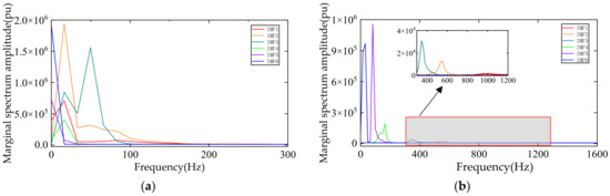
Figure 1.
Comparison of marginal spectra after Hilbert transformation for two decomposition methods: (a) Marginal spectrum of EMD decomposition; (b) Marginal spectrum of VMD decomposition.
A comparison of the two spectra reveals that, under the same number of decomposition levels, VMD effectively suppresses mode mixing and demonstrates significantly greater decomposition stability. This makes it particularly suitable for capturing the non-stationary characteristics of transient signals like inrush currents. The VMD results not only accurately reconstruct the time-frequency structure of the original signal but also carry clear physical interpretations. This provides a reliable foundation for the subsequent multi-domain feature extraction (e.g., from time and frequency domains) essential for accurate identification.
2.2. ReliefF Algorithm
The ReliefF algorithm, an enhancement of the classic Relief method introduced by Kononenko in 1994, supports both multi-class classification and regression tasks. Its core mechanism evaluates a feature’s importance by dynamically calculating its weight, which reflects the feature’s ability to distinguish between classes. A higher positive weight indicates a stronger discriminative power for the feature, while a negative weight suggests that the feature may be noisy or misleading for classification and should be considered for removal [26]. The algorithm employs a k-nearest neighbor strategy to estimate these weights, which enhances its robustness against noise and missing data. As a filter-based method, ReliefF can rapidly process high-dimensional datasets without the need for model training, offering a practical balance of efficiency and utility. In this work, the number of nearest neighbors kis set to 5, and Euclidean distance is used as the proximity measure.
2.3. VMD–ReliefF Feature Selection Algorithm
To enable efficient feature screening and classification optimization for inrush currents, this paper proposes an outcome-driven VMD-ReliefF feature selection framework. This method dynamically selects the optimal decomposition level (K) and the optimal feature subset by iterating through different decomposition depths and evaluating cross-validation results, significantly reducing computational complexity while preserving the physical interpretability of the features. Its core advantages are twofold:
- (1)
- Dynamically adaptive full-scale VMD decomposition
Conventional VMD optimization methods predefine the number of decomposition levels (K) for a single, typical inrush current signal using metrics like frequency-band separation or energy entropy. This often leads to poor compatibility with fault current signals and a disconnect from the ultimate classification objective. To address this, we propose a novel, full-scale decomposition strategy. By comparing the cross-validation results across different decomposition levels, this strategy dynamically adapts the decomposition depth directly to the signal characteristics. It moves away from the traditional practice of setting K a priori based solely on inrush current data, thereby avoiding a mismatch with the decomposition needs of fault currents. Driven by classification performance, it effectively balances the noise introduced by over-decomposition against the information loss from under-decomposition, ensuring the decomposition level consistently matches the signal complexity and classification requirements.
- (2)
- Lightweight feature selection
For each candidate decomposition level K (corresponding to a K × 12 dimensional feature space), a two-stage screening process is employed. First, the ReliefF algorithm calculates a weight for each feature, ranking them in descending order of their contribution to class discrimination. Features that are noise-sensitive or redundant across frequency bands are filtered out, retaining only the top 12 highest-weighted features. Subsequently, a forward stepwise feature selection strategy is applied to this refined set. Starting from an empty subset, features are added one at a time. For each candidate subset, the EEFO algorithm optimizes the SVM parameters. A classification model is then trained and evaluated, allowing for the identification of the specific feature subset that yields the best classification performance for the given decomposition level K.
3. Multi-Feature Analysis and Extraction
To address the limitations of single-feature identification methods, which are often susceptible to variations in fault types and initial system conditions, leading to incomplete characterization and inadequate adaptability, this paper proposes a multidimensional joint feature extraction strategy. This approach ensures a comprehensive depiction of the data by simultaneously mining information from multiple domains, including the time domain, frequency domain, and nonlinear characteristics.
3.1. Time-Domain Feature Analysis and Extraction
For the time-domain features, the selection process balanced the complementary nature of dimensional and dimensionless metrics with the specific requirements of identification. Six dimensional features were ultimately chosen: maximum value, minimum value, variance, energy, root amplitude, and root mean square (RMS) value. Three dimensionless features were also selected: kurtosis, skewness, and waveform factor. Dimensional features directly characterize the signal’s amplitude strength and energy distribution, making them sensitive to operational fluctuations. In contrast, dimensionless features capture the morphological information of the waveform, possessing inherent robustness to amplitude scale and operational variations, thereby effectively mitigating the impact of such fluctuations on the classification model. These two categories of features complement each other: the former provides information on overall energy and amplitude differences, while the latter focuses on the detailed temporal shape. This combination enables high-accuracy, high-stability fault classification across diverse operating conditions. The nine extracted time-domain features and their corresponding formulas are presented in Table 1.

Table 1.
Time-domain feature variables and their mathematical expressions.
3.2. Frequency-Domain Feature Analysis and Extraction
Magnetizing inrush currents are typically rich in second- and higher-order harmonics, while fault currents are predominantly composed of the fundamental component. Leveraging this distinction, features extracted from the signal’s Fourier transform provide a critical basis for identification. This work selects two core frequency-domain features: the spectral centroid and the frequency variance. The spectral centroid, defined as the weighted average of the frequency spectrum with respect to its energy, characterizes the central tendency of the signal’s energy distribution. The frequency variance quantifies the spread of spectral energy around the centroid, reflecting the width and complexity of the harmonic distribution. These two features are complementary: the centroid indicates the trend of energy concentration, while the variance measures the breadth and dispersion of harmonics. Together, they furnish a reliable basis for signal classification. The two extracted frequency-domain features and their calculation formulas are listed in Table 2.
Table 2.
Frequency-domain feature variables and their mathematical expressions.
3.3. Nonlinear Time-Domain Feature
Sample Entropy (SampEn) serves as a metric for quantifying the complexity of a time series. It is defined as the negative natural logarithm of the conditional probability that two sequences of length m, which are initially similar (within a tolerance r), remain similar when extended to length m + 1. A lower SampEn value indicates higher self-similarity and regularity within the sequence, whereas a higher value signifies greater complexity and randomness. Applying SampEn to each decomposed IMF allows for an effective characterization of the stochasticity and regularity inherent in each mode. This provides a significant advantage in capturing the complex fluctuation patterns of non-stationary signals like inrush currents. In this work, the embedding dimension mis set to 2, and the tolerance is defined as 0.2 times the standard deviation of the respective IMF component, ensuring the threshold adapts to the amplitude of each mode.
4. Excitation Inrush Current Identification Method Based on EEFO–SVM
4.1. Electric-Eel Foraging Optimization Algorithm
During group hunting, electric eels first swim in circular patterns to herd fish into a compact aggregation, often referred to as a “prey ball.” They then coordinate a simultaneous, high-voltage electric discharge for a collective attack. This strategy maximizes the group’s gain by spatially compressing the prey and synchronizing the discharge, significantly increasing the energy acquisition rate per unit time, particularly within dense fish schools [27].
The Electric Eel Foraging Optimization algorithm is a meta-heuristic that simulates the collective social predation behaviors of electric eels [28]. It models four primary behavioral phases: Interaction, Resting, Migration, and Hunting. In this work, the algorithm parameters are configured as follows: a population size of 40, a maximum iteration count of 200, an optimization variable dimension of 2 (corresponding to the SVM parameters C and γ), and a Lévy flight parameter β of 1.5.
- Parameter Initialization: Define the population size, maximum number of iterations, search space boundaries, and problem dimensionality;
- Population Initialization: Initialize the positions of all individuals in the population and compute their corresponding fitness values;
- Interaction Phase: When the energy factor , electric eels engage in interaction behavior and update their positions;
- Resting Phase: When the energy factor , electric eels engage in resting behavior, update their positions, and update the optimal solution;
- Migration Phase: When the energy factor satisfies , the electric eel performs migration behavior, updating its position and the optimal solution;
- Hunting Phase: When the energy factor satisfies , the electric eel performs hunting behavior, updating its position and the optimal solution;
- Termination: The algorithm terminates when the stopping criterion (maximum iteration count or convergence threshold) is satisfied, and the best-found solution is output.
4.2. Support Vector Machine
The Support Vector Machine, introduced by Vapnik and Cortes in 1995, is grounded in the principle of structural risk minimization. It determines an optimal classification boundary by solving a convex optimization problem to find the maximum-margin hyperplane. This approach is particularly effective for problems involving small samples, high-dimensional nonlinearity, and the avoidance of local minima. Unlike traditional neural networks that rely on empirical risk minimization, the generalization performance of an SVM is highly dependent on two key parameters: the penalty factor C and the kernel function parameter γ. The parameter C governs the trade-off between model complexity and misclassification tolerance, while γ controls the influence radius of individual training samples. However, the model is sensitive to the settings of these parameters, where inappropriate values can easily lead to overfitting or underfitting [29,30,31,32]. In this work, the Radial Basis Function (RBF) is selected as the kernel. The parameters C and γ are treated as optimization variables, with their search spaces defined as [0.01, 100] and [0.01, 1000], respectively.
The Electric Eel Foraging Optimization algorithm exhibits strong global search capability and possesses mechanisms to escape local optima, allowing it to effectively balance exploration and exploitation. Therefore, this study employs the EEFO algorithm to optimize the SVM parameters, aiming to enhance the final classification performance and model stability.
4.3. Inrush Current Identification Based on VMD–ReliefF–EEFO–SVM
The flowchart of the excitation inrush current identification method based on VMD–ReliefF–EEFO–SVM is shown in Figure 2. The main steps of the identification procedure are as follows:
Step 1: Waveform Data Acquisition—Simulation models for excitation inrush and fault currents are constructed in MATLAB 2020b. Waveforms are generated under varying system impedances, phase angles, residual flux values, secondary winding connection configurations, and fault types to obtain representative excitation inrush and fault current signals.
Step 2: VMD Decomposition and Mode Number Optimization—All acquired waveforms are subjected to Variational Mode Decomposition. The decomposition level K is varied from 1 to 7, and the optimal number of modes is dynamically determined based on subsequent classification performance.
Step 3: Multi-Dimensional Feature Extraction—For each extracted IMF, the following features are computed:
- Time-domain features: maximum, minimum, variance, etc.;
- Frequency-domain features: spectral centroid, spectral variance;
- Nonlinear features: sample entropy.
These features are concatenated to form a complete feature vector.
Step 4: Data Processing—All feature vectors are normalized and stratified by class, then divided into training and testing sets.
Step 5: Preliminary Feature Selection via ReliefF—For each feature set corresponding to a decomposition level K, feature weights are computed using the ReliefF algorithm and ranked in descending order. The top 12 features are retained, while noise-sensitive and cross-frequency redundant features are discarded.
Step 6: Based on the features pre-screened in Step 5, a forward stepwise feature selection strategy is employed. Starting from an empty set, features are added one at a time. For each candidate feature subset, the corresponding 5-fold cross-validation classification accuracy is calculated and serves as the evaluation criterion. This process iteratively identifies the optimal feature combination for the current decomposition level. By comparing the results across all candidate levels, the global optimal decomposition level and its corresponding optimal feature subset are ultimately determined.
Step 7: The optimized SVM model is evaluated using the held-out test set. The test set data is input into the model, and key performance metrics—including classification accuracy, confusion matrix, precision, and recall—are calculated to provide a comprehensive assessment of the model’s generalization capability.

Figure 2.
Flowchart of the inrush current identification model based on VMD-ReliefF-EEFO-SVM.
Figure 2.
Flowchart of the inrush current identification model based on VMD-ReliefF-EEFO-SVM.

5. Simulation Verification
To validate the accuracy and reliability of the proposed method for inrush current identification, a simulation model for generating both magnetizing inrush and short-circuit fault currents, as illustrated in Figure 3, was developed in MATLAB 2020b. The phase-A current on the primary side was selected as the analysis target. The modeled transformer has a rated capacity of 31.5 MVA, a voltage ratio of 35/10 kV, and a Y/D11 connection. Its equivalent circuit parameters, in per-unit values, are as follows: primary winding resistance Rp = 0.002 pu and leakage inductance Lp = 0.08 pu; secondary winding resistance Rs = 0.002 pu and leakage inductance Ls = 0.08 pu; magnetizing branch resistance Rm = 500 pu and inductance Lm = 500 pu. The core’s nonlinear saturation effect is modeled using the saturation characteristic curve defined by the points [0, 0; 0.0024, 1.2; 1.0, 1.52] (pu). The transformer equivalent circuit model is illustrated in Figure 4.
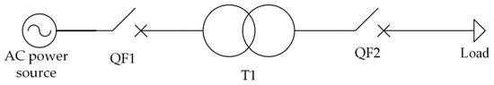
Figure 3.
Simulation model for magnetizing inrush and short-circuit fault currents.
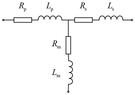
Figure 4.
Transformer equivalent model.
Magnetizing inrush currents in transformers primarily occur under two conditions: when the transformer is energized on no-load, and as a recovery inrush following the clearance of an external fault. Given the multitude of factors influencing inrush current characteristics, this study focuses on the impact of the source closing (point-on-wave) angle, residual flux, system impedance, and the connection type of the transformer’s secondary winding.
For fault conditions within the transformer, the study examines internal faults and the scenario of energizing the transformer into an existing internal fault. The influencing factors considered for fault currents include the fault type, fault inception angle, system impedance, and the secondary winding connection. A summary of the multi-scenario simulation cases is provided in Table 3.
Table 3.
Summary of multi-scenario simulation cases.
5.1. Waveform Analysis
5.1.1. Magnetizing Inrush Current
The simulation results for a closing angle of 0°, a residual flux of 0 pu, a system impedance of 1 + j10 Ω, and a transformer winding connection of Y/D11 are presented in Figure 5.
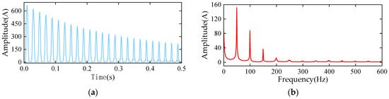
Figure 5.
Simulated waveform of magnetizing inrush current with corresponding amplitude spectrum: (a) Phase-A Waveform of Magnetizing Inrush Current; (b) Amplitude Spectrum of Magnetizing Inrush Current.
In Figure 5a, the Phase A magnetizing inrush current waveform exhibits an initial peak of approximately 600 A at the moment of energization. This is followed by a sharp inrush pulse in each subsequent power frequency cycle. The amplitude of these pulses decays exponentially over time. Between consecutive peaks, the current nearly returns to zero, creating distinct “current-zero” intervals. This pattern indicates strong damping during the oscillatory process, which effectively suppresses the current between cycles. The overall time-domain waveform also exhibits a slight superimposed resonance, visible as minor ringing adjacent to each main peak, reflecting the interaction between the system’s inductive and resistive components.
Figure 5b shows the corresponding amplitude spectrum. The dominant peak is at the fundamental power frequency (50 Hz), with subsequent harmonic peaks at 100 Hz, 150 Hz, and so forth, whose amplitudes decrease successively. This confirms that while the inrush current is dominated by the fundamental component, it contains substantial harmonic content. This spectral characteristic aligns perfectly with the physical mechanism illustrated in Figure 6: the sinusoidally varying flux linkage forces the core’s operating point to cyclically enter the nonlinear saturation region, distorting the magnetizing current into a peaked waveform. It is precisely this nonlinear magnetization process due to core saturation that generates the prominent harmonics, predominantly the 2nd and 3rd.
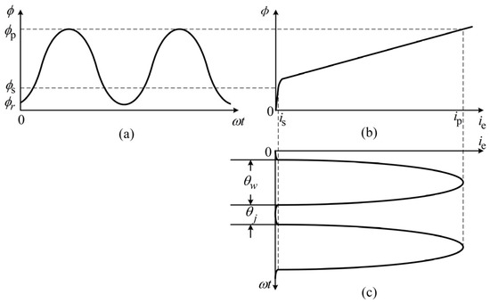
Figure 6.
Generation mechanism of magnetizing inrush current: (a) Flux Trajectory during No-Load Energization; (b) Magnetization Curve; (c) Magnetizing Inrush Current.
Furthermore, several low-amplitude components are observable at frequencies below the fundamental. These correspond directly to the decaying envelope of the transient inrush current in Figure 5a. Their physical origin is the gradual dissipation of inrush energy as core losses (hysteresis and eddy currents) and winding resistance losses, which generates low-frequency oscillatory signals. From the overall spectral energy distribution, it is evident that energy is highly concentrated at the 50 Hz fundamental and its integer multiples. This concentration in the frequency domain corroborates the time-domain observation of a single sharp pulse per cycle in Figure 5a.
The root cause of these spectral features lies in the mutation of the equivalent circuit model triggered by core saturation. From the modeling perspective, saturation fundamentally manifests as a dynamic, drastic reduction in the magnetizing inductance, . In the linear region, remains relatively constant. Upon entering saturation, its value plummets, mathematically corresponding to a sharp decline in the slope of the magnetization curve (). This leads to two critical consequences: First, a much larger magnetizing current is required to sustain the same alternating flux change, resulting in the high-amplitude inrush. Second, the effective magnetic coupling between the primary and secondary windings is severely weakened. Consequently, a greater portion of the input electrical energy is not transferred as power but is instead converted into core losses (hysteresis and eddy currents) and resistive (Joule) heating in the windings.
Therefore, the significant harmonic components in the inrush signal are essentially a manifestation of energy redistribution in the frequency domain caused by the nonlinear variation of . Conversely, the low-frequency decaying components are a direct reflection of the impeded energy transfer pathway following the drop in , where substantial electrical energy is converted into internal losses.
5.1.2. Fault Current
The simulation results for a three-phase short-circuit fault under the conditions of a fault inception angle of 0°, a system impedance of 1 + j10 Ω, and a transformer winding connection of Y/D11 are presented in Figure 7.
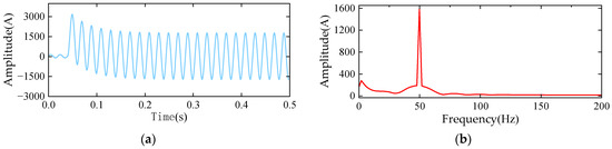
Figure 7.
Simulated waveform of fault current with corresponding amplitude spectrum: (a) Phase-A Waveform of Internal Fault; (b) Amplitude Spectrum of Internal Fault.
Figure 7a shows that at the instant of fault occurrence, the current surges rapidly to approximately 3000 A, accompanied by a noticeable DC offset. This DC component then decays swiftly, and the current transitions into a power-frequency (50 Hz) oscillation. The amplitude gradually stabilizes around 1800 A. This evolution—from an initial high-magnitude impulse with a DC component to a predominantly pure power-frequency sinusoid in the later stage—reflects the characteristic fast transient decay governed by the combined effect of the system’s resistance and reactance following the fault.
In the corresponding amplitude spectrum (Figure 7b), the 50 Hz fundamental component overwhelmingly dominates, with its magnitude far exceeding all other frequency components. The amplitudes of higher-order harmonics are minimal and essentially negligible. This indicates that after the brief transient period, the fault current quickly converges to an almost pure power-frequency sinusoidal wave. The small-magnitude peak near 0 Hz corresponds to the rapidly decaying transient DC offset observed in the time domain. Overall, the amplitude spectrum confirms two key signatures of the fault current: (1) a short-duration high-magnitude impulse with a DC offset exists at the initial stage due to transient superposition, and (2) after a brief transient decay, the current rapidly settles into a steady-state condition dominated by the 50 Hz fundamental, with no significant higher-order harmonic interference.
5.2. Multidimensional Feature Analysis
From the simulation model, 364 sets of magnetizing inrush current waveforms and 516 sets of fault current waveforms were generated, as previously described. Following the conditions specified in Section 5.1, the inrush current closing angles were varied to 0° and 90°, and the three-phase short-circuit fault inception angles were similarly set to 0° and 90°. Single-phase-to-ground faults under corresponding conditions were also included. The feature data extracted from the complete set of waveforms is summarized in Table 4.
Table 4.
Multidimensional features of magnetizing inrush current and fault current.
Observations from the table indicate a degree of crossover or even overlap in the peak amplitude between the inrush and the two types of fault currents. From the perspectives of energy and variance, the inrush current is markedly lower than the fault currents. This suggests that fault currents possess greater volatility and higher energy levels, whereas the inrush current exhibits weaker fluctuations and a more concentrated distribution. The effective magnitude metrics (Root Amplitude and RMS value) further corroborate this conclusion, showing that the effective magnitude of fault currents is significantly greater than that of the inrush current.
Higher-order statistics reveal differences in waveform morphology and temporal symmetry. The kurtosis of the inrush current is approximately three times that of the fault currents, indicating the presence of more sharp, impulsive peaks in its waveform. Regarding skewness, the inrush current exhibits a larger absolute value, reflecting poorer temporal symmetry, while the fault currents demonstrate a distribution closer to symmetry. The waveform factor is higher for the inrush current, signifying that its peak value constitutes a more prominent proportion relative to its mean, whereas the fault current waveforms tend to be more uniform.
In terms of spectral characteristics, the dominant frequency of the inrush current is located closer to, yet slightly above, the fundamental frequency, and its spectral distribution is more dispersed. In contrast, the dominant frequencies for both three-phase and single-phase-to-ground fault currents are heavily concentrated near the fundamental frequency. Notably, the spectral distribution of the three-phase fault current is significantly influenced by the fault inception angle, being more dispersed at 0° and highly concentrated at 90°. Regarding the temporal complexity metric, the sample entropy of the fault currents is approximately double that of the inrush current, indicating richer dynamic features and stronger temporal irregularity, while the inrush current’s time series appears simpler and more regular.
The analysis above demonstrates that magnetizing inrush currents and fault currents exhibit significant differences across various feature dimensions. However, crossover or overlap exists in some features, making discrimination based on any single feature highly susceptible to misjudgment. Therefore, it is necessary to adopt a multi-domain, multi-dimensional feature fusion strategy that comprehensively considers time-domain, frequency-domain, and complexity features to enhance the robustness of the classification model and the reliability of identification.
5.3. Model Validation
5.3.1. Determination of Optimal K Value
EMD was first applied to the inrush current signal, yielding six IMFs. To enhance the richness of the feature set and ensure the coverage of information from multiple frequency bands, the proposed method based on VMD was tested by systematically traversing decomposition levels (K) from 1 to 7.
To mitigate the risk of overfitting and ensure the generalization capability of the method, a strict data isolation protocol was adhered to during model development. The entire dataset was first split into a training set and a completely independent test set in a 7:3 ratio. The test set was sequestered and was not involved in any parameter optimization or feature selection process. Within the training set, the optimal VMD decomposition level and feature subset were determined through a nested procedure: For each candidate decomposition level, the Relief-F algorithm was employed for initial feature screening, followed by a forward stepwise feature selection strategy. The criterion for selection at each step was the 5-fold cross-validation classification accuracy. This iterative process identified the optimal feature combination for that specific decomposition level. By comparing the cross-validation performance across all levels, the global optimal decomposition level and its corresponding optimal feature subset were finally established.
As shown in Table 5, the EEFO-SVM model achieved its best classification accuracy for distinguishing inrush currents from fault currents when the VMD decomposition level was set to 5 and the feature subset size was 10. The selected optimal feature subset includes: the Root Amplitude of IMF4, the Sample Entropy of IMF3, the Sample Entropy of IMF5, the Frequency Variance of IMF4, the Spectral Centroid of IMF4, the Waveform Factor of IMF5, the RMS value of IMF4, the Waveform Factor of IMF4, the Sample Entropy of IMF2, and the Frequency Variance of IMF1.
Table 5.
Cross-validation accuracy and number of features corresponding to different decomposition levels.
The results indicate that the selected optimal feature subset encompasses information from various aspects of different IMF components. IMF4 was selected multiple times, suggesting that its corresponding mid-frequency band effectively reflects the differences between inrush and fault currents in terms of amplitude, spectral concentration, and peak characteristics. The Sample Entropy values of IMF3, IMF5, and IMF2 capture the differences in stochastic complexity within their respective components. Conversely, the Frequency Variance of IMF1 highlights the distinct energy distribution in the highest frequency band. By combining time-domain, frequency-domain, and nonlinear features from different components, the model is equipped to comprehensively discern the inherent differences between the two types of currents.
5.3.2. Comparative Study on Feature Extraction Methods Based on EMD and Adaptive VMD
In the feature extraction process based on EMD, the decomposition results are susceptible to mode mixing, where components of different frequencies may be blended into a single mode. This can prevent the effective separation and extraction of subtle yet critical signal features, thereby compromising the classifier’s stability and generalization capability in noisy environments. In contrast, the adaptive VMD method decomposes non-stationary waveforms into a set of narrow-band, non-overlapping modal components. This capability allows it to effectively highlight local details and spectral features beneficial for fault discrimination, thereby enhancing feature distinctiveness and improving the time-frequency representation of the signal. A comparative analysis of the classification performance using features derived from EMD versus adaptive VMD can further validate the advantage of adaptive VMD in improving the model’s discriminative power and robustness.
A comparison of Figure 6b and Figure 8a clearly demonstrates the superior classification accuracy achieved by the model utilizing features extracted via adaptive VMD, compared to the one using EMD-based features. In Figure 8a, 107 inrush current instances were correctly identified, with only 3 misclassified as fault currents. For fault currents, 150 were correctly identified, with 4 misclassified as inrush. The total number of misclassifications was 7, resulting in a classification accuracy of 97.35% and an F1-Score of 96.83%. In contrast, Figure 8b shows 99 correct inrush identifications with 11 misclassifications, and 144 correct fault current identifications with 10 misclassifications. The total misclassifications increased to 21, yielding a lower accuracy of 92.05% and a lower F1-Score of 90.45%.
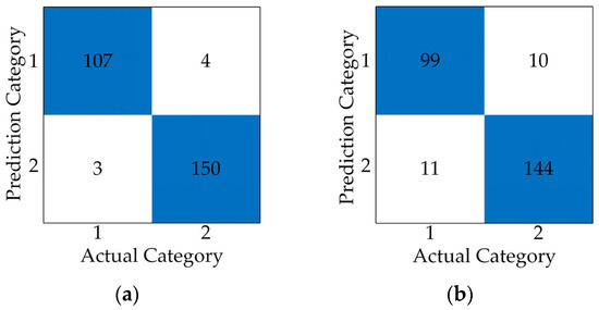
Figure 8.
Comparison of feature extraction methods based on EMD and adaptive VMD: (a) Confusion Matrix Based on Adaptive VMD Decomposition; (b) Confusion Matrix Based on EMD Decomposition.
These results indicate that the features obtained from adaptive VMD decomposition more accurately capture the fundamental distinctions between inrush and fault currents, effectively reducing classification errors and thereby enhancing the overall identification performance.
5.3.3. Comparison of Optimization Algorithms
To validate the optimization capability of the EEFO algorithm, a comparative test was conducted against the Whale Optimization Algorithm (WOA) and the Marine Predators Algorithm (MPA). The results are presented in Figure 9 and Table 6.
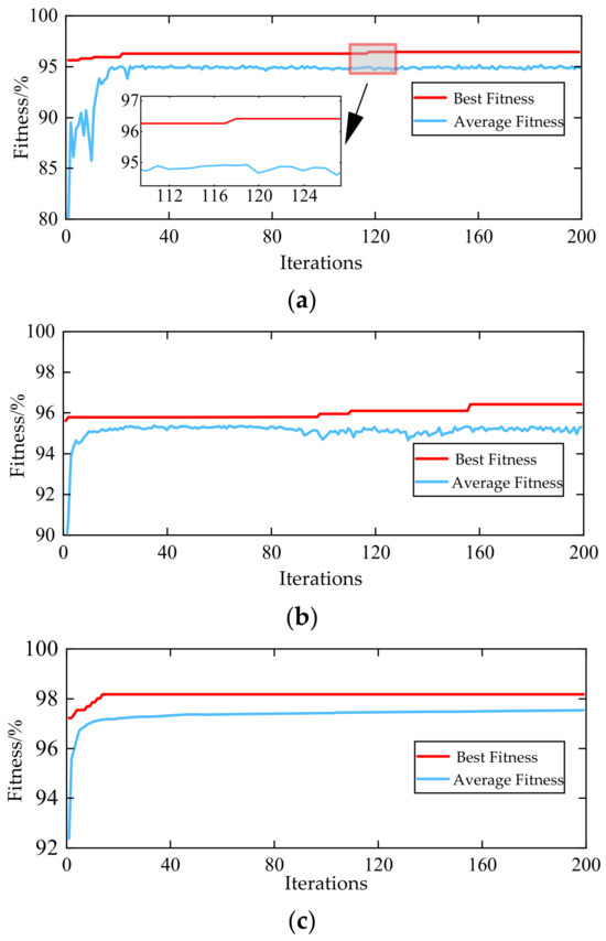
Figure 9.
Comparison of SVM parameter optimization using different algorithms: (a) Optimization search curve of WOA; (b) Optimization search curve of MPA; (c) Optimization search curve of EEFO.
Table 6.
Identification results of different optimization algorithms.
As shown in Figure 9, WOA, MPA, and EEFO converged to their optimal training accuracy at the 118th, 157th, and 14th iteration, respectively. EEFO demonstrated a significantly faster convergence rate than the other two algorithms.
The comparative data in Table 6 indicate that the EEFO-SVM model delivers superior performance in inrush current identification compared to WOA-SVM and MPA-SVM. EEFO-SVM achieved a Recall of 97.27% and a Specificity of 97.4%, outperforming WOA-SVM (94.55%, 95.45%) and MPA-SVM (91.82%, 95.45%). This demonstrates the enhanced capability of the EEFO algorithm in discriminating between inrush and fault currents. In terms of the F1-Score, EEFO-SVM reached 96.83%, significantly higher than WOA-SVM (94.12%) and MPA-SVM (92.66%), reflecting a better balance between precision and recall, which effectively reduces both false positives and false negatives. Regarding overall diagnostic accuracy, EEFO-SVM attained 97.35%, again surpassing WOA-SVM (95.08%) and MPA-SVM (93.94%). These results validate the stronger global search capability and robustness of the EEFO algorithm.
In summary, while all three models are capable of effectively distinguishing inrush currents from fault currents, the EEFO-SVM model demonstrates the best performance across all evaluated metrics. This confirms its superiority and practical feasibility for multi-feature inrush current identification, providing substantial support for enhancing the reliability of transformer differential protection.
5.3.4. Comparison of Methods
This section conducts a performance comparison between the proposed method and two state-of-the-art methods under identical experimental conditions. A fair assessment is ensured by employing exactly the same training and testing datasets for all methods. As detailed in Table 7, the proposed method demonstrates superior performance across all key metrics. It achieves a recall of 97.27%, surpassing the 93.64% of the RT-BSWT + SVM method and the 94.55% of the PSO-SVDD method. While maintaining a high recall, its specificity reaches 97.4%, which is comparable to the 98.05% of PSO-SVDD and significantly better than the 94.81% of RT-BSWT + SVM. Furthermore, the proposed method attains the highest scores in both the F1-score (96.83%)—which balances precision and recall—and the overall diagnostic accuracy (97.35%). These comparative results indicate that the proposed identification framework, which integrates adaptive VMD decomposition, ReliefF-based feature selection, and EEFO-optimized SVM, offers more robust and reliable performance in accurately discriminating between magnetizing inrush currents and internal faults.
Table 7.
Detection of methods comparison.
5.3.5. Computational Efficiency Analysis
During the offline model construction phase, the computational cost is concentrated on the global search for optimal parameters. The exhaustive evaluation of VMD across a full scale of decomposition levels (K = 1–7) required a total time of 10,780.34 s. Building upon this, a single run of the EEFO for SVM parameter tuning took an average of 328.56 s. Determining the optimal decomposition level and the optimal feature subset necessitated 84 such EEFO optimization runs.
Although the overall offline optimization process is time-consuming, it constitutes a one-time model development cost. In practical engineering applications, this stage can be executed efficiently on high-performance computing platforms using parallel processing, thus not impacting the real-time performance of the subsequent online identification system.
In the online protection application stage, all model parameters—the VMD decomposition level (K = 5) and the optimal 10-dimensional feature subset—are predetermined. The identification process for a new sample is thus streamlined into three steps: performing VMD decomposition with fixed parameters, extracting the predefined 10-dimensional features from the resultant IMFs, and feeding the feature vector into the pre-trained EEFO-SVM model for classification. Measurements indicate that the core computational burden lies in the VMD decomposition, taking approximately 2.96 s, while feature extraction and classification decision require about 10.72 milliseconds. The total identification time currently exceeds the millisecond-level operating time limit required for power system relay protection.
To meet real-time requirements, several engineering strategies can be pursued in future implementations. These include porting the VMD algorithm to embedded platforms, rewriting the core computational routines in C/C++, employing fixed-point arithmetic for acceleration, or designing dedicated hardware acceleration modules. Through these targeted optimizations, the total time for a single identification is expected to be reduced to within the protection time limit, demonstrating the framework’s potential for practical online deployment.
6. Conclusions
To address the issue of magnetizing inrush current generated during transformer no-load energization, which often leads to maloperation of differential protection, this paper proposes a multi-feature intelligent identification method based on adaptive VMD. The method abandons the conventional practice of pre-setting parameters based on signal metrics. Instead, it directly uses classification accuracy as the optimization objective to achieve adaptive tuning of the VMD decomposition level. On this basis, features from the time domain, frequency domain, and nonlinear characteristics are fused and extracted. A ReliefF algorithm combined with a forward stepwise selection strategy is employed to construct an optimal feature subset characterized by low redundancy and high discriminative power. Simulation results demonstrate that the proposed method achieves accurate identification of inrush currents under various operating condition changes, including closing angle, residual flux, system impedance, and winding connection types, exhibiting good robustness and adaptability.
The present study is primarily based on simulation data. While the method’s effectiveness has been verified under typical conditions, its practical engineering applicability requires further validation as it has not yet been tested with actual field operational data. Future research can be advanced in the following two directions: First, field recording data can be collected from transformers of different models and operating environments to empirically validate the generalization capability of the proposed method. Second, further analysis can be conducted by combining the transformer equivalent model to deeply investigate the quantitative relationship between core losses, winding losses, and harmonic content during the inrush current transient process. This would enhance the model’s physical interpretability while improving identification accuracy, thereby providing a more solid theoretical foundation for protection setting and fault diagnosis.
Author Contributions
Conceptualization, P.D. and L.Y.; methodology, P.D. and L.Y.; software, L.Y. and H.Z.; validation, P.D., L.Y. and H.Z.; writing—original draft preparation, L.Y. and H.Z.; writing—review and editing, P.D., L.Y. and H.Z. All authors have read and agreed to the published version of the manuscript.
Funding
This research received no external funding.
Data Availability Statement
The raw data supporting the conclusions of this article will be made available by the authors on request.
Conflicts of Interest
The authors declare no conflicts of interest.
References
- Hao, C.; Liu, X. Do New Energy Vehicles Reduce Carbon Emissions? A Quasi-Natural Experiment Using China’s Ten Cities, Thousand Vehicles Project. Energy 2025, 335, 138061. [Google Scholar] [CrossRef]
- Chen, Z.-M.; Xiong, Q.; Duan, J.; Ma, J.; Chen, Z.; Guo, S. AI Carbon Footprint in China Sets to Double Post-2030 Carbon Peaking. Energy Econ. 2025, 150, 108880. [Google Scholar] [CrossRef]
- Darwish, H.; AlHmoud, I.W.; Turlapaty, A.C.; Gokaraju, B. Predicting the Future Climate: Integrating Renewable Energy and Machine Learning to Address Temperature and GHG Emissions. Energy Rep. 2025, 14, 2399–2419. [Google Scholar] [CrossRef]
- Zhang, Y.; Tang, H.; Li, H.; Wang, S. Integration and Interaction of Next-Generation AI-Focused Data Centers with Smart Grids and District Energy Systems: The State-of-the-Art, Opportunities and Challenges. Renew. Sustain. Energy Rev. 2025, 224, 116097. [Google Scholar] [CrossRef]
- Camarena-Martinez, D.; Huerta-Rosales, J.R.; Amezquita-Sanchez, J.P.; Granados-Lieberman, D.; Olivares-Galvan, J.C.; Valtierra-Rodriguez, M. Variational Mode Decomposition-Based Processing for Detection of Short-Circuited Turns in Transformers Using Vibration Signals and Machine Learning. Electronics 2024, 13, 1215. [Google Scholar] [CrossRef]
- Hamilton, R. Analysis of Transformer Inrush Current and Comparison of Harmonic Restraint Methods in Transformer Protection. IEEE Trans. Ind. Appl. 2013, 49, 1890–1899. [Google Scholar] [CrossRef]
- Sung, B.C.; Kim, S. Accurate Transformer Inrush Current Analysis by Controlling Closing Instant and Residual Flux. Electr. Power Syst. Res. 2023, 223, 109638. [Google Scholar] [CrossRef]
- Nagpal, M.; Martinich, T.G.; Moshref, A.; Morison, K.; Kundur, P. Assessing and Limiting Impact of Transformer Inrush Current on Power Quality. IEEE Trans. Power Deliv. 2006, 21, 890–896. [Google Scholar] [CrossRef]
- Chiesa, N.; Høidalen, H.K. Novel Approach for Reducing Transformer Inrush Currents: Laboratory Measurements, Analytical Interpretation and Simulation Studies. IEEE Trans. Power Deliv. 2010, 25, 2609–2616. [Google Scholar] [CrossRef]
- Cano-González, R.; Bachiller-Soler, A.; Rosendo-Macías, J.A.; Álvarez-Cordero, G. Controlled Switching Strategies for Transformer Inrush Current Reduction: A Comparative Study. Electr. Power Syst. Res. 2017, 145, 12–18. [Google Scholar] [CrossRef]
- Gunda, S.K.; Dhanikonda, V.S.S.S.S. Discrimination of Transformer Inrush Currents and Internal Fault Currents Using Extended Kalman Filter Algorithm (EKF). Energies 2021, 14, 6020. [Google Scholar] [CrossRef]
- Samet, H.; Shadaei, M.; Tajdinian, M. Statistical Discrimination Index Founded on Rate of Change of Phase Angle for Immunization of Transformer Differential Protection against Inrush Current. Int. J. Electr. Power Energy Syst. 2022, 134, 107381. [Google Scholar] [CrossRef]
- Mishra, P.; Swain, A.; Pradhan, A.K.; Bajpai, P. Sequence Current-Based Inrush Detection in High-Permeability Core Transformers. IEEE Trans. Instrum. Meas. 2023, 72, 3534509. [Google Scholar] [CrossRef]
- Babaei, Z.; Moradi, M. Novel Method for Discrimination of Transformers Faults from Magnetizing Inrush Currents Using Wavelet Transform. Iran. J. Sci. Technol. Trans. Electr. Eng. 2021, 45, 803–813. [Google Scholar] [CrossRef]
- Etumi, A.A.A.; Anayi, F.J. Current Signal Processing-Based Methods to Discriminate Internal Faults from Magnetizing Inrush Current. Electr. Eng. 2021, 103, 743–751. [Google Scholar] [CrossRef]
- Chai, J.; Zheng, Y.; Pan, S. Rotating Phasor-Based Algorithm for the Identification of Inrush Currents of Three-Phase Transformers. Electr. Power Syst. Res. 2023, 214, 108936. [Google Scholar] [CrossRef]
- Simões, L.D.; Costa, H.J.D.; Aires, M.N.O.; Medeiros, R.P.; Costa, F.B.; Bretas, A.S. A Power Transformer Differential Protection Based on Support Vector Machine and Wavelet Transform. Electr. Power Syst. Res. 2021, 197, 107297. [Google Scholar] [CrossRef]
- Li, Z.; Xv, N.; Chen, X.; Zhang, Y.; He, A.; Jiao, Z. Blocking Method with PSO-SVDD for Differential Protection of Power Transformer. Electr. Power Syst. Res. 2024, 237, 111016. [Google Scholar] [CrossRef]
- Sun, Y.; Li, S.; Wang, X. Bearing Fault Diagnosis Based on EMD and Improved Chebyshev Distance in SDP Image. Measurement 2021, 176, 109100. [Google Scholar] [CrossRef]
- Amarouayache, I.I.E.; Saadi, M.N.; Guersi, N.; Boutasseta, N. Bearing Fault Diagnostics Using EEMD Processing and Convolutional Neural Network Methods. Int. J. Adv. Manuf. Technol. 2020, 107, 4077–4095. [Google Scholar] [CrossRef]
- Mejia-Barron, A.; Valtierra-Rodriguez, M.; Granados-Lieberman, D.; Olivares-Galvan, J.C.; Escarela-Perez, R. The Application of EMD-Based Methods for Diagnosis of Winding Faults in a Transformer Using Transient and Steady State Currents. Measurement 2018, 117, 371–379. [Google Scholar] [CrossRef]
- Li, H.; Liu, T.; Wu, X.; Chen, Q. An Optimized VMD Method and Its Applications in Bearing Fault Diagnosis. Measurement 2020, 166, 108185. [Google Scholar] [CrossRef]
- Zhou, J.; Xiao, M.; Niu, Y.; Ji, G. Rolling Bearing Fault Diagnosis Based on WGWOA-VMD-SVM. Sensors 2022, 22, 6281. [Google Scholar] [CrossRef]
- Dragomiretskiy, K.; Zosso, D. Variational Mode Decomposition. IEEE Trans. Signal Process. 2014, 62, 531–544. [Google Scholar] [CrossRef]
- Wang, Y.; Liu, F.; Jiang, Z.; He, S.; Mo, Q. Complex Variational Mode Decomposition for Signal Processing Applications. Mech. Syst. Signal Process. 2017, 86, 75–85. [Google Scholar] [CrossRef]
- Bing, W.; Xiong, H. Fault Diagnosis Technique Based on Multi-Domain Features and RelifF-Bayes-KNN in Rolling Bearing. Nonlinear Dyn. 2025, 113, 12985–13000. [Google Scholar] [CrossRef]
- Zhao, W.; Wang, L.; Zhang, Z.; Fan, H.; Zhang, J.; Mirjalili, S.; Khodadadi, N.; Cao, Q. Electric Eel Foraging Optimization: A New Bio-Inspired Optimizer for Engineering Applications. Expert Syst. Appl. 2024, 238, 122200. [Google Scholar] [CrossRef]
- Abdelwahab, S.A.M.; El-Rifaie, A.M.; Hegazy, H.Y.; Tolba, M.A.; Mohamed, W.I.; Mohamed, M. Optimal Control and Optimization of Grid-Connected PV and Wind Turbine Hybrid Systems Using Electric Eel Foraging Optimization Algorithms. Sensors 2024, 24, 2354. [Google Scholar] [CrossRef]
- Chauhan, V.K.; Dahiya, K.; Sharma, A. Problem Formulations and Solvers in Linear SVM: A Review. Artif. Intell. Rev. 2019, 52, 803–855. [Google Scholar] [CrossRef]
- Rushdi Saleh, M.; Martín-Valdivia, M.T.; Montejo-Ráez, A.; Ureña-López, L.A. Experiments with SVM to Classify Opinions in Different Domains. Expert Syst. Appl. 2011, 38, 14799–14804. [Google Scholar] [CrossRef]
- Chorowski, J.; Wang, J.; Zurada, J.M. Review and Performance Comparison of SVM- and ELM-Based Classifiers. Neurocomputing 2014, 128, 507–516. [Google Scholar] [CrossRef]
- Cherkassky, V.; Ma, Y. Practical Selection of SVM Parameters and Noise Estimation for SVM Regression. Neural Netw. 2004, 17, 113–126. [Google Scholar] [CrossRef] [PubMed]


Disclaimer/Publisher’s Note: The statements, opinions and data contained in all publications are solely those of the individual author(s) and contributor(s) and not of MDPI and/or the editor(s). MDPI and/or the editor(s) disclaim responsibility for any injury to people or property resulting from any ideas, methods, instructions or products referred to in the content. |
© 2026 by the authors. Licensee MDPI, Basel, Switzerland. This article is an open access article distributed under the terms and conditions of the Creative Commons Attribution (CC BY) license.