Article

A Reproducible Benchmarking Framework for Differential Evolution Variants in Wind Turbine Controller Tuning

by
Adrián Geovanny Urgilés Rojas
*,
Nicolás Dueñas Vargas
and
Julio César Zambrano Abad
Research Group on Interaction, Robotics and Automation (GIIRA), Universidad Politécnica Salesiana, Cuenca 010105, Ecuador
*
Author to whom correspondence should be addressed.
Energies 2026, 19(18), 4420; https://doi.org/10.3390/en19184420 (registering DOI)
Submission received: 9 August 2026 / Revised: 5 September 2026 / Accepted: 10 September 2026 / Published: 18 September 2026
(This article belongs to the Special Issue Advances in Wind Turbine Optimization and Control)

Abstract

Modern wind turbines require effective control strategies to maximize energy capture under partial-load conditions while maintaining generator-speed and power regulation above the rated wind speed. This study proposes and applies a controlled and reproducible benchmarking framework for evaluating classical Differential Evolution (DE) variants in the tuning of Proportional–Integral–Derivative (PID) and Proportional–Integral–Derivative–Accelerative (PIDA) controllers for a nonlinear model of the National Renewable Energy Laboratory 5-MW reference wind turbine. Twenty classical DE variants were assessed using a fixed-seed initialization strategy, unified simulation procedures, consistent objective-function definitions, and region-specific optimization settings applied uniformly to all variants within each operating region. The controllers were evaluated in Region 2, where maximum power point tracking is required, and Region 3, where generator speed and electrical power must be regulated under above-rated wind conditions. Their generalization performance was subsequently evaluated in simulation using a measured wind-speed profile obtained from a Supervisory Control and Data Acquisition system. In Region 2, under the considered fixed-seed configuration, the DE-tuned controller achieving the lowest objective-function value reduced the objective function by approximately 2.93% compared with the baseline PID controller, indicating a moderate improvement. In Region 3, the PIDA controller tuned with the DE variant yielding the lowest objective-function value achieved a reduction of up to 92% relative to the baseline controller, demonstrating a substantially greater benefit under above-rated operation. However, validation using the measured wind profile indicated that some controllers with favorable tuning-stage results showed signs of overfitting and reduced generalization performance. Overall, the results indicate that the suitability of the controller structure and DE configuration depends on the wind turbine operating region and highlight the importance of controlled, reproducible optimization procedures and validation beyond the tuning scenario in wind turbine controller design.

1. Introduction

The regulation of nonlinear dynamical systems operating under varying conditions remains a fundamental challenge in control engineering. Strong nonlinearities, coupled subsystems, and operating-region-dependent dynamics often limit the effectiveness of analytical tuning rules and linearization-based design methodologies. In such environments, controller performance may degrade significantly when disturbance rejection, operating-point variations, and multi-objective requirements must be simultaneously addressed.
These challenges are particularly relevant in modern energy systems, aerospace applications, and complex electromechanical plants, where high-performance regulation must be maintained despite nonlinear interactions between subsystems and varying environmental conditions [1,2]. In such scenarios, achieving robust disturbance rejection, stability across multiple operating regimes, and satisfactory transient behavior simultaneously becomes a demanding control-design task.
Large-scale wind turbines constitute a representative example of nonlinear multi-regime systems. Their dynamics arise from the interaction of aerodynamic, mechanical, and electrical subsystems, leading to strong nonlinear behavior and operating-region-dependent control objectives [3,4,5,6]. In addition, studies on flexible rotating blades have highlighted the relevance of nonlinear vibration dynamics, delayed feedback, and active vibration suppression in rotating structures, further illustrating the complexity associated with blade dynamics and their control [7,8]. In particular, during high-load operation, control objectives are primarily associated with disturbance rejection around regulated operating points rather than classical reference tracking. These characteristics increase tuning complexity and reduce the effectiveness of conventional linear design tools. Consequently, the systematic regulation of wind turbines provides a demanding and realistic context for evaluating advanced controller-tuning methodologies [9,10].
Despite the nonlinear nature of wind turbine dynamics, industrial control systems frequently rely on relatively simple feedback controllers due to their ease of implementation, robustness, and interpretability. Among these, the Proportional–Integral–Derivative (PID) controller remains the dominant industrial standard. Its widespread adoption is largely attributed to its intuitive structure, low implementation cost, and the existence of well-established tuning rules such as the Ziegler–Nichols and Cohen–Coon methods [11].
However, the structural simplicity of PID controllers can limit achievable performance in systems exhibiting high-order dynamics, significant nonlinearities, or strong coupling between subsystems. In such situations, the limited number of adjustable parameters may restrict the ability to shape closed-loop dynamics effectively. To overcome these limitations, several extensions of the PID structure have been proposed in the literature to increase design flexibility and improve dynamic compensation capabilities.
Among these extended structures, the Proportional Integral Derivative Accelerative (PIDA) controller, originally introduced in [12], incorporates an additional zero in the controller transfer function through the inclusion of an accelerative term. Compared with the conventional PID structure, this additional term increases the degrees of freedom available for shaping the closed-loop dynamics. In this sense, PIDA and related higher-order derivative controllers have been reported to improve transient response and disturbance-rejection capability in processes with demanding dynamic characteristics, such as high-order, delayed, or oscillatory plants [13,14].
From a physical perspective, this feature is relevant to wind turbine control because rapid wind-induced variations can lead to transient speed deviations and oscillatory responses in the regulated system. The accelerative action may therefore provide additional dynamic compensation, potentially contributing to reduced overshoot, faster regulation around the operating point, and improved disturbance attenuation. This is especially important in above-rated operation, where pitch control is the main mechanism for regulating generator speed and mitigating aerodynamic disturbances [15].
However, the increased dynamic compensation capability of the PIDA controller also introduces additional tuning challenges. If the accelerative term is not properly filtered or tuned, it may increase sensitivity to high-frequency components, measurement noise, or aggressive control actions, which can affect closed-loop robustness and actuator effort [16,17,18]. Therefore, the practical use of PIDA controllers requires a systematic tuning strategy capable of balancing performance improvement, stability preservation, and robustness under different operating conditions. As a result, PIDA controllers have attracted attention in applications where enhanced dynamic compensation is desirable [19,20,21]. Nevertheless, unlike PID controllers, PIDA structures lack consolidated and systematically validated tuning methodologies, particularly in nonlinear multi-regime environments. This absence of structured tuning approaches motivates the exploration of optimization-based methods.
In recent decades, metaheuristic optimization algorithms have emerged as effective alternatives for controller tuning in nonlinear and high-dimensional systems [22,23,24]. Among these techniques, Differential Evolution (DE) has received considerable attention due to its algorithmic simplicity, robustness, and strong performance in continuous search spaces [25,26,27,28]. Since its original formulation, DE has evolved into a broad family of variants derived from modifications to mutation and crossover strategies. These variants exhibit distinct exploration–exploitation characteristics and convergence behaviors, leading to performance differences across optimization problems [29,30,31,32]. Additionally, sensitivity to manually tuned control parameters in classical variants has motivated the development of adaptive formulations such as CODE, JADE, jDE, and SaDE [33,34], as well as empirical investigations into parameter-setting strategies [35].
Despite the widespread application of DE in controller tuning, existing comparative studies often evaluate only limited subsets of algorithm variants or rely on mathematical benchmark functions that do not fully represent the dynamic complexity of nonlinear control systems. Furthermore, differences in experimental protocols—including random initialization, simulation environments, cost-function definitions, search-space settings, and implementation procedures—can hinder reproducibility and complicate direct comparison among reported results [36,37,38]. Consequently, a methodological gap remains in the availability of controlled and reproducible benchmarking procedures for systematically evaluating a broad set of classical DE variants in realistic nonlinear controller-tuning problems. Under heterogeneous experimental conditions, it becomes difficult to distinguish performance differences associated with the algorithmic configuration from those introduced by the experimental design itself.
To address this methodological gap, this work proposes a controlled and reproducible DE-based benchmarking framework for nonlinear multi-region controller-tuning problems. The framework establishes a structured experimental protocol based on fixed-seed initialization, predefined search bounds, consistent performance-index definitions, and unified simulation procedures. Within each operating region, all DE variants are evaluated using the same optimization configuration, initial population, objective function, controller structure, and simulation scenario, while region-specific settings are consistently maintained across variants. A total of twenty classical DE variants are evaluated under this protocol, providing a common experimental basis for reproducible and traceable performance comparison.
The original contribution of this work lies in the unified application of this controlled and reproducible benchmarking framework to the evaluation of classical DE variants for PID and PIDA controller tuning in a nonlinear wind turbine system. By applying a common experimental protocol within each operating region, the framework reduces the influence of initialization and implementation-related inconsistencies, providing a controlled basis for examining the convergence behavior and resulting controller performance associated with different mutation and crossover strategies. In addition, the study evaluates the suitability of PID and PIDA controller structures across partial- and above-rated operating regions and subsequently examines their generalization performance in simulation using a measured SCADA wind-speed profile. This additional evaluation makes it possible to identify cases in which favorable tuning-stage performance does not translate into satisfactory behavior under different wind conditions, revealing signs of overfitting. Therefore, the reported results provide insight into the combined influence of the DE configuration, controller structure, and wind turbine operating region under the considered experimental scenarios.
The remainder of this article is organized as follows. Section 2 describes the wind turbine model and its operating regions. Section 3 presents the controller structure and the optimization problem formulation. Section 4 introduces the proposed benchmarking framework. Section 5 details the simulation setup and experimental protocol. Section 6 discusses the comparative results. Finally, Section 7 summarizes the main conclusions and outlines directions for future research.

2. Wind Turbine Modeling and Operating Regions

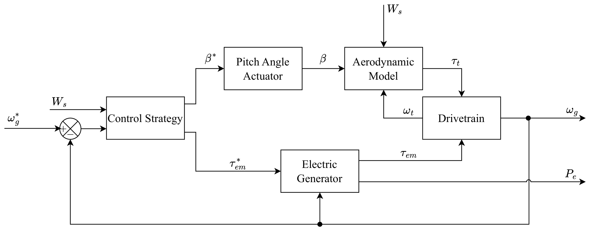
The wind turbine model considered in this work is the National Renewable Energy Laboratory (NREL) 5-MW reference turbine [39], which is widely adopted as a benchmark in large scale wind turbine control studies. The aerodynamic, mechanical, pitch actuator, and generator parameters follow the original NREL specification, with a slight deviation in the rated wind speed due to differences in the aerodynamic representation, yielding a comparable maximum power coefficient and a rated wind speed of 11.6 m / s . Figure 1 provides a schematic representation of the overall wind turbine system, depicting the interconnection of its subsystems and the associated input–output signals. The physical interpretation of these variables is reported in Table 1.
The controlled variable is the generator angular speed ω g , while the control inputs correspond to the pitch-angle reference β and the electromagnetic torque reference τ e m . The electrical power output P e depends on both the generator speed and electromagnetic torque, and its regulation is therefore determined by the operating-region-specific control strategy. Each subsystem of the wind turbine model is characterized by a specific set of parameters that govern its dynamic behavior and interactions within the overall system. In the following, all subsystems are systematically described. The numerical values of the model parameters, adopted from the NREL reference turbine, are summarized in Table 2, which provides a consolidated overview of the model parameterization.

2.1. Aerodynamic Model

The aerodynamic subsystem models the conversion of wind kinetic energy into mechanical power and torque. The aerodynamic power is computed using Equation (1).
P t = 1 2 ρ π r 2 v 3 C p ( λ , β ) ,
where λ = ω t r / v denotes the tip-speed ratio. The power coefficient C p ( λ , β ) is computed using Equations (2) and (3) following the formulation proposed in [40]. The corresponding aerodynamic torque is then obtained as τ t = P t / ω t .
C p ( λ , β ) = 0.5176 116 λ i 0.4 β 5 e 21 / λ i + 0.0068 λ
1 λ i = 1 λ + 0.08 β 0.035 β 3 + 1
The auxiliary variable λ i represents an effective tip-speed ratio introduced for the empirical approximation of C p ( λ , β ) .

2.2. Pitch Actuator Model

The pitch actuator adjusts the blade pitch angle β and is modeled as a simplified second-order system, given by:
β ¨ = ω n 2 β 2 ζ ω n β ˙ + ω n 2 β ,
where β is the controller-generated pitch reference, ω n the natural frequency, and  ζ the damping ratio. Physical constraints are enforced according to Table 2.

2.3. Drivetrain Model

The mechanical drivetrain is modeled using a two-mass representation that captures the torsional interaction between the turbine and the generator through a flexible shaft and an ideal gearbox. The turbine and generator inertias, J t and J g , rotate at angular speeds ω t and ω g , respectively, and are coupled by a shaft with stiffness K s and damping D s . The applied torques include the aerodynamic torque τ t acting on the turbine, the shaft torque τ s transmitted through the drivetrain, and the electromagnetic torque τ e m generated by the electrical machine. The drivetrain dynamics are described by Equations (5)–(7).
J t d d t ( ω t ) = τ t τ s D t ω t
J g d d t ( ω g ) = τ s N g τ e m D g ω g
τ s = K s θ t θ g N g + D s ω t ω g N g

2.4. Electrical Generator Model

The electrical subsystem is modeled using a simplified first-order representation of the electromagnetic torque dynamics, as described by Equation (8).
τ ˙ e m = 1 τ g τ e m + 1 τ g τ e m ,
The parameter τ e m denotes the torque reference, whereas τ g represents the electrical time constant. The electrical power output is computed as follows:
P e = η τ e m ω g ,
where η denotes the overall electromechanical efficiency. Torque and electrical-power saturation effects are neglected in the present model, allowing transient values beyond nominal rated conditions during simulation.

2.5. Wind Turbine Operating Regions

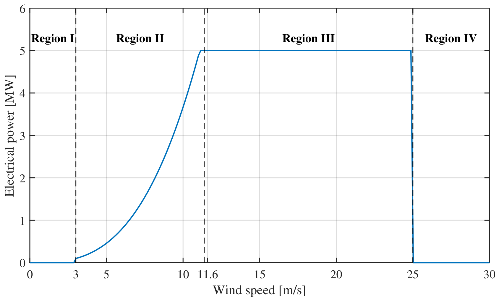
Wind turbine operation is typically divided into four regions, as illustrated in Figure 2.
In Region 2, the control objective is to support Maximum Power Point Tracking (MPPT) operation by regulating the generator speed through the electromagnetic torque while maintaining the pitch angle at its optimal value. This strategy aims to keep the turbine operating near the aerodynamic condition associated with maximum power extraction under partial-load conditions. In Region 3, corresponding to operation above the rated wind speed, the objective is to maintain the generator speed and electrical power near their rated values by adjusting the blade pitch while holding the electromagnetic torque constant.

3. Controller Structure and Problem Formulation

3.1. PIDA Controller Structure and Formulation

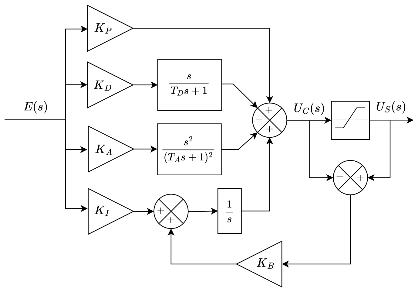
The transfer function of the PIDA controller is given by Equation (10), which incorporates low-pass filters in the derivative and acceleration actions to limit high-frequency amplification and improve the practical implementation of these terms.
C ( s ) = K P + K I 1 s + K D s T D s + 1 + K A s 2 ( T A s + 1 ) 2
The parameters K P , K I , K D , and  K A denote the proportional, integral, derivative, and acceleration gains, respectively, while T D and T A are the time constants of the low-pass filters associated with the derivative and acceleration actions, ensuring a proper transfer function. To mitigate integrator windup in the presence of actuator saturation, the PIDA controller incorporates an anti-windup compensation scheme based on the back-calculation method. The resulting controller structure is shown in Figure 3.
The gain K B is defined in Equation (11) and is obtained as the geometric mean of the time constants associated with the integral, derivative, and acceleration actions [41]. This gain weights the difference between the computed control signal U C ( s ) and the saturated control signal U S ( s ) , facilitating integrator discharge and mitigating windup effects when actuator saturation occurs.
K B = 1 K D K A K I K P 3

3.2. Optimization Problem Formulation for Controller Tuning

The DE algorithm is employed to search for the controller parameter vector that minimizes the selected objective function within the prescribed search bounds:
min θ J ( θ )
where θ = [ K P , K I , K D , K A , T D , T A ] denotes the decision-variable vector for the PIDA controller. For the PID structure, the corresponding parameter vector is obtained by excluding the acceleration-related parameters K A and T A . In both cases, the optimization problem is formulated as a bounded continuous search, with each controller parameter constrained within predefined limits.
The objective function is formulated according to the specific control objective and dynamic characteristics associated with each operating region. Integral performance indices provide a practical basis for this formulation because they quantify the accumulated tracking or regulation error over the complete simulation horizon. However, the choice of a particular index directly affects the relative importance assigned to error magnitude and persistence. Absolute-error criteria, such as the Integral of Absolute Error (IAE) and the Integral of Time-weighted Absolute Error (ITAE), penalize the error proportionally to its magnitude, whereas squared-error criteria, such as the Integral of Squared Error (ISE) and the Integral of Time-weighted Squared Error (ITSE), assign a comparatively larger penalty to high-magnitude deviations. In addition, time-weighted indices progressively increase the contribution of errors that remain present as the response evolves. Therefore, the selected objective function is defined according to the dominant control requirement of each operating region.
In Region 2, the control objective is primarily associated with generator-speed reference tracking required by the Maximum Power Point Tracking (MPPT) strategy. Under this operating condition, the objective function must quantify the accumulated tracking error over the different operating points without allowing short-duration, high-magnitude deviations to dominate the optimization process. For this reason, the Integral of Absolute Error (IAE), defined in Equation (13), is adopted. Its linear dependence on the error magnitude provides a direct measure of the total tracking deviation accumulated over the simulation horizon.
I A E ( θ ) = 0 t | e ( t ) | d t
Compared with the ISE criterion, the IAE does not amplify large instantaneous errors through quadratic weighting. Although squared-error indices are useful when the reduction of large transient deviations is the dominant design objective, their increased sensitivity to error magnitude may cause isolated transients to contribute disproportionately to the total cost. In the Region 2 tracking problem considered in this work, a proportional accumulation of the tracking error is therefore preferred because it provides a more uniform assessment of the response over the complete operating sequence.
In Region 3, the control objective changes from reference tracking to generator-speed regulation under above-rated wind conditions, where variations in wind speed act primarily as external disturbances. In this case, the duration of the regulation error becomes particularly relevant because deviations that persist after a disturbance indicate slower recovery of the rated operating condition. Accordingly, the Integral of Time-weighted Absolute Error (ITAE), defined in Equation (14), is selected. The time-weighting factor progressively increases the penalty associated with persistent errors, thereby favoring responses in which deviations from the rated generator speed are attenuated within shorter time intervals.
I T A E ( θ ) = 0 t t | e ( t ) | d t
Although ITSE also introduces a time-dependent weighting, it additionally applies a quadratic penalty to the error magnitude. Consequently, large transient deviations receive a substantially greater contribution to the objective function. ITAE retains the desired sensitivity to error persistence without introducing this additional quadratic amplification, which makes it suitable for the disturbance-rejection objective considered in Region 3, where both the magnitude and duration of the regulation error are relevant.
It should also be noted that IAE, ISE, ITAE, and ITSE are error-based performance indices and therefore do not explicitly penalize control effort. Consequently, a lower integral error index represents improved tracking or regulation performance according to the selected criterion, but it does not necessarily imply minimum actuator activity. Explicit consideration of control effort would require the inclusion of additional terms associated with the magnitude or variation of the electromagnetic-torque and pitch-angle commands, together with appropriate normalization and weighting factors. Such a formulation would introduce an additional trade-off between tracking accuracy and actuator activity. In the present study, a scalar error-based objective function is deliberately retained to provide a transparent and reproducible optimization criterion directly associated with the primary control objective of each operating region. The controller architecture additionally incorporates filtered derivative and acceleration actions and back-calculation anti-windup compensation, as described in Section 3, while the explicit incorporation of control-effort criteria remains a possible extension of the proposed framework.

4. Differential Evolution-Based Tuning Framework

4.1. Differential Evolution Fundamentals

Differential Evolution is a stochastic, population-based optimization algorithm based on mutation and crossover operators. Algorithm 1 presents the canonical workflow of the DE algorithm. It begins by defining the control parameters, including the population size N p , the mutation scaling factor F, and the crossover probability C r . An initial population of candidate solutions is then randomly generated within the prescribed search bounds. At each generation G, for each target vector x i , G , a mutant vector v i , G is generated according to the selected mutation strategy. Subsequently, each mutant vector is crossed with its corresponding target vector to produce a trial vector u i , G . A one-to-one selection scheme is then applied, whereby the trial vector replaces the target only if it yields a lower cost value. This iterative process continues until the maximum number of generations N g is reached or another predefined stopping criterion is satisfied.
Different variants of the DE algorithm arise from the specific design of its mutation and crossover operators, which directly shape the search dynamics and convergence behavior. Although the overall optimization workflow remains unchanged, alternative formulations of these operators lead to distinct algorithmic behaviors. Accordingly, DE variants are commonly denoted using the standard DE/x/y/z notation, where x identifies the mutation strategy, y denotes the number of difference vectors used in the mutation process, and z specifies the crossover scheme. The mutation operator typically employs one or two difference vectors ( y = 1 or y = 2 ), while the crossover mechanism is commonly implemented using either a binomial (bin) or an exponential (exp) scheme.
Algorithm 1 Standard DE algorithm
  1:
Define control parameters: N p , F, C r , and stopping criterion
  2:
Initialize population { x i , 0 } i = 1 N p randomly within the search bounds
  3:
Set generation counter G 0
  4:
while stopping criterion not satisfied do
  5:
      for  i = 1 to N p  do
  6:
            Generate v i , G according to the selected mutation strategy
  7:
            Generate trial vector u i , G by crossing v i , G with x i , G
  8:
            if  f ( u i , G ) f ( x i , G )  then
  9:
                  x i , G + 1 u i , G
10:
            else
11:
                  x i , G + 1 x i , G
12:
            end if
13:
      end for
14:
       G G + 1
15:
end while
16:
return best solution found in the final population
In this study, a total of 20 classical DE variants are considered, obtained by combining five mutation strategies (best, rand, current-to-best, current-to-rand, and rand-to-best), two differentiation orders ( y = 1 , 2 ), and two crossover operators (bin and exp). The complete set of analyzed variants is summarized in Table 3, and the same variants are consistently applied in both Region 2 and Region 3 to ensure a fair and homogeneous benchmarking framework.

4.2. Controlled Initialization and Fair Comparison Strategy

Due to the stochastic nature of Differential Evolution (DE), optimization outcomes depend not only on the algorithmic configuration of each variant but also on the random processes involved during the search. Randomness affects several stages of DE, including initial-population generation, individual selection for mutation, and the probabilistic decisions associated with crossover. Consequently, when different DE variants are evaluated under independently generated stochastic conditions, part of the observed performance differences may be influenced by random sampling effects in addition to the mutation strategy, differentiation order, and crossover scheme.
To promote a controlled and reproducible comparison, this study adopts a fixed-seed random-number generation strategy. For each operating region and controller architecture, the same random seed and random-number generator configuration are used for all evaluated DE variants. This procedure ensures that each optimization experiment can be reproduced from a predefined stochastic initialization and that all variants are evaluated from a common initial population under the corresponding experimental scenario. By controlling the initialization procedure, the framework reduces one source of experimental variability and provides a more consistent basis for comparing the behavior of the different DE configurations.
Reproducibility is implemented in MATLAB through the rng function, using a fixed positive integer seed and a predefined generator type. Before executing each set of comparable optimization runs, the random number generator is initialized explicitly, ensuring that the initial population and subsequent stochastic operations can be reproduced exactly. In contrast, if the seed is not specified, MATLAB initializes the generator using time-dependent information from the system clock, which leads to non-reproducible results.
This controlled initialization strategy is particularly relevant because the study compares multiple DE variants applied to the same controller-tuning problem. Within each operating region, the wind profile, simulation horizon, controller structure, parameter bounds, objective function, population size, number of generations, stopping criterion, and initial population are kept unchanged across variants. Region-specific settings are therefore consistently applied to all DE configurations, providing a common experimental basis for the comparison. Under these conditions, differences in convergence behavior and resulting controller performance can be examined while reducing the influence of initialization and implementation-related inconsistencies.
The fixed-seed protocol is intended to ensure reproducibility and controlled comparison under the defined experimental conditions. Accordingly, the reported results characterize the behavior of the evaluated DE variants within the considered stochastic realization and operating scenarios rather than providing a statistical characterization across independent random realizations. Nevertheless, the protocol enables the reported controller parameters, convergence curves, and performance indices to be regenerated and provides a transparent basis for extending the benchmark to additional DE variants, controller structures, or repeated stochastic evaluations in future studies.

5. Simulation Setup and Experimental Design

This section outlines the simulation environment and experimental design adopted to ensure a consistent and reproducible application of the DE-based tuning framework in Regions 2 and 3 of the wind turbine, addressing the region-specific control problems defined in Section 2.5. All simulations were implemented in the Simulink environment of MATLAB R2024b, where the system model, control architecture, and optimization procedures were fully integrated. The simulation setup, operating conditions, performance metrics, and optimization parameters are described in the following subsections. To promote transparency and reproducibility, the complete implementation of the proposed framework, including the Simulink models and optimization scripts, is publicly available through an external repository [42].

5.1. Simulation Environment

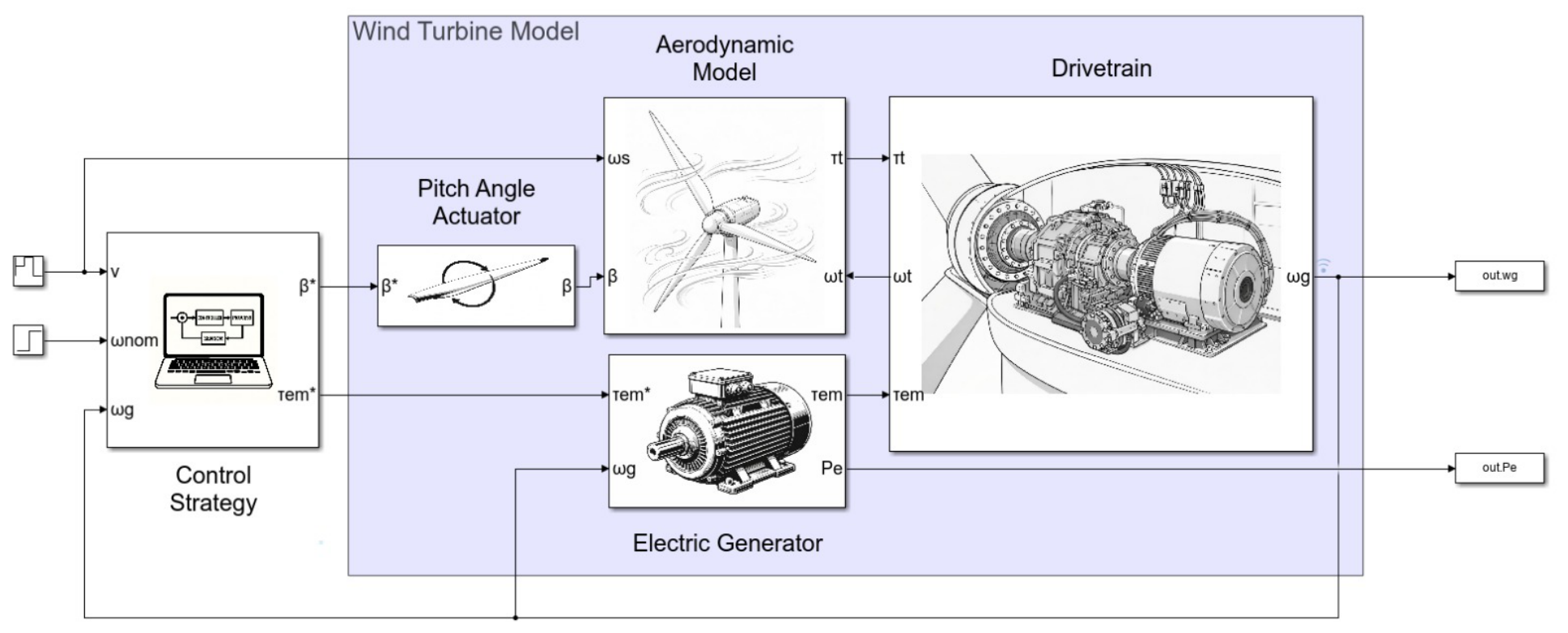
The wind turbine model was implemented according to the mathematical formulation presented in Section 2. All simulations were performed using a variable-step solver with MATLAB/Simulink automatic solver selection. The relative tolerance was set to 1 × 10 3 , whereas the absolute tolerance, maximum step size, minimum step size, and initial step size were automatically determined by Simulink. Zero-crossing detection was configured using the local block settings with the nonadaptive algorithm. The same numerical solver configuration was maintained across all DE variants within each operating region to ensure consistent numerical integration conditions throughout the benchmarking procedure. The complete Simulink implementation of the wind turbine system, including all subsystems described in Section 2, is shown in Figure 4, which illustrates the block-level functional architecture of the nonlinear model and the corresponding signal flow among subsystems. The diagram represents the closed-loop operation of the system under normal operating conditions, where wind speed and reference signals are processed by the control strategy to generate pitch-angle and electromagnetic-torque references according to the current operating region.
Generative artificial intelligence was used solely to create the illustrative graphical elements embedded within the Simulink subsystem blocks shown in Figure 4. These elements were generated using ChatGPT, GPT-5.5 (OpenAI), for visual representation only. The block diagram, model architecture, subsystem structure, signal interconnections, mathematical formulation, model parameters, simulation data, and numerical results were developed by the authors and were not generated or modified using artificial intelligence. All AI-generated graphical elements were reviewed by the authors before their incorporation into the figure.
To evaluate the proposed tuning framework, two independent simulation experiments were designed, each corresponding to a distinct operating region of the wind turbine.
In Region 2, the process variable is the generator angular speed, whose reference is a step sequence with values [ 94.11 , 122.9 , 37.64 ] rad / s , enforced through electromagnetic torque regulation. These values are selected to excite system nonlinearities by combining sub-nominal, nominal, and low-speed operating points. The corresponding wind-speed profile is [ 7.5 , 11.4 , 3 ] m / s , with transitions every 25 s and a total simulation time of 75 s .
In Region 3, the process variable is held constant at the rated generator speed by regulating the blade pitch angle, with initial conditions ω t i = 1.267 rad / s and ω g i = 122.9 rad / s . The wind-speed profile is defined as [ 12 , 16 , 24.9 , 18 ] m / s , introducing disturbances of varying amplitudes across the full operating range, with transitions every 125 s and a total simulation time of 500 s .
All simulations were performed using the control structure shown in Figure 3, implemented in discrete time through the Backward–Euler formulation with a controller sampling time of 0.05 s. A common discrete control architecture is employed across the operating regions, with the active controller and its corresponding parameters selected according to the current wind-turbine operating condition. This implementation avoids the use of independent continuous-time controller blocks and provides a uniform numerical formulation for the PID/PIDA control actions. Moreover, the discrete implementation prevents the numerical slowdown typically associated with continuous-time tuning when the filter time constants T D and T A approach zero. In such cases, the derivative and acceleration actions are evaluated in the discrete domain, thereby ensuring stable and computationally efficient simulations.
During simulations involving wind profiles that span multiple operating regions, the active control strategy is selected according to the instantaneous wind speed. Region 2 is active for wind speeds below the rated value of 11.6 m / s , whereas Region 3 becomes active at and above the rated wind speed. In Region 2, the blade pitch reference is maintained at its optimal value and generator-speed regulation is performed through the electromagnetic-torque command. In Region 3, the electromagnetic torque is maintained at its rated value and generator-speed regulation is performed through the blade-pitch command. The present implementation uses a direct switching boundary at the rated wind speed and does not incorporate an additional hysteresis band. This choice provides a simple and reproducible region-selection mechanism within the proposed benchmarking framework. In applications where the wind speed repeatedly fluctuates around the rated operating point, a hysteresis band or an additional supervisory switching strategy could be incorporated to reduce frequent transitions between operating regions.
The controllers associated with Regions 2 and 3 maintain independent internal states. When one operating region becomes inactive, the states associated with its controller are retained but are not updated until that region becomes active again. This prevents the inactive integral action from continuously accumulating error outside its corresponding operating region. During active operation, each controller independently applies the back-calculation anti-windup mechanism described in Section 3, using the difference between the unsaturated and saturated control signals to correct the integral action. No explicit synchronization of the internal states between the torque and pitch controllers is performed, and no dedicated bumpless-transfer mechanism is implemented. Consequently, the apparent continuity of the control signals observed during the SCADA-based validation should not be interpreted as the result of an explicit bumpless-transfer strategy. Furthermore, because the validation figures represent a complete day of operation, their time scale does not resolve individual switching events. Dedicated hysteresis, state synchronization, and bumpless-transfer strategies therefore remain possible extensions for real-time or industrial implementations.

5.2. DE Parameter Settings and Reproducibility

This subsection summarizes the configuration of the DE algorithm used for controller tuning in both operating regions. To ensure reproducibility and fair benchmarking, a deterministic setup was adopted, with fixed random-number generation and identical initial populations across all DE variants. The main DE parameters, described in Section 4.1, are listed in Table 4.
The observed differences between operating regions stem from their distinct dynamic characteristics. In Region 2, the system exhibits relatively simple and less sensitive dynamics, resulting in a smoother objective-function landscape. Under these conditions, exploration—primarily governed by the DE mutation factor F and crossover rate C r —is more effective and allows convergence to be achieved within a smaller number of generations.
In contrast, Region 3 is characterized by stronger nonlinearities and higher sensitivity to control actions, mainly due to the interaction between pitch dynamics and aerodynamic effects. Such characteristics typically lead to a more rugged and sensitive search space, in which excessive exploration may degrade convergence or induce unstable candidate solutions. Consequently, the admissible level of exploration must be reduced, resulting in a more constrained and exploitation-oriented search process.
Despite these differences, identical random-number generation settings are employed in all cases, using a fixed seed of 1 and the twister generator, in order to ensure reproducibility. The only stopping criterion considered is the completion of the predefined number of generations, and the cost function corresponds to that defined in SubSection 3.2. The search space for Region 2 is defined as
{ K P , K I , K D , K A [ 4 × 10 4 , 0 ] ; T D , T A [ 0 , 1 ] } ,
whereas for Region 3 it is given by
{ K P , K I , K D , K A [ 5 , 0 ] ; T D , T A [ 0 , 3 ] } .
The search bounds were selected based on the order of magnitude of the control signals associated with each operating region.
In terms of computational cost, the optimization process is mainly determined by the number of iterations required to tune each DE variant. In this context, a simulation refers to the complete optimization process of one DE variant, whereas an iteration refers to the evaluation of a single candidate individual through a complete closed-loop Simulink execution of the nonlinear wind turbine model.
The number of iterations per simulation was determined from the population size and the maximum number of generations defined in Table 4. Based on these parameters, each DE variant requires approximately 5000 iterations in Region 2 and 12,000 iterations in Region 3. Each iteration in Region 2 evaluates 75 s of turbine operation, while each iteration in Region 3 evaluates 500 s. Therefore, the computational demand is considerably higher in Region 3 because each simulation involves both a larger number of iterations and a longer simulation horizon for each evaluated individual.
Using a single processor core, the execution time of one complete simulation ranged from approximately 40 to 60 min in Region 2, depending on the evaluated DE variant. In Region 3, the execution time increased to approximately 3.5 to 4 h per variant. The developed framework also includes the option of enabling MATLAB’s Parallel Computing Toolbox. When this option is activated, the execution time can be reduced by up to four times, since several iteration loops can be evaluated simultaneously using a larger number of processor cores.
All simulations were executed in MATLAB/Simulink R2024b on a workstation equipped with an Intel(R) Core(TM) i7-10750H CPU @ 2.60 GHz, 6 cores, 32 GB RAM, an NVIDIA GeForce RTX 2060 GPU with 6 GB of dedicated memory, a 64-bit x64-based operating system, and Windows 11 version 24H2.

6. Results and Discussion

6.1. Region 2 Results

6.1.1. Optimization Performance of DE Variants in Region 2

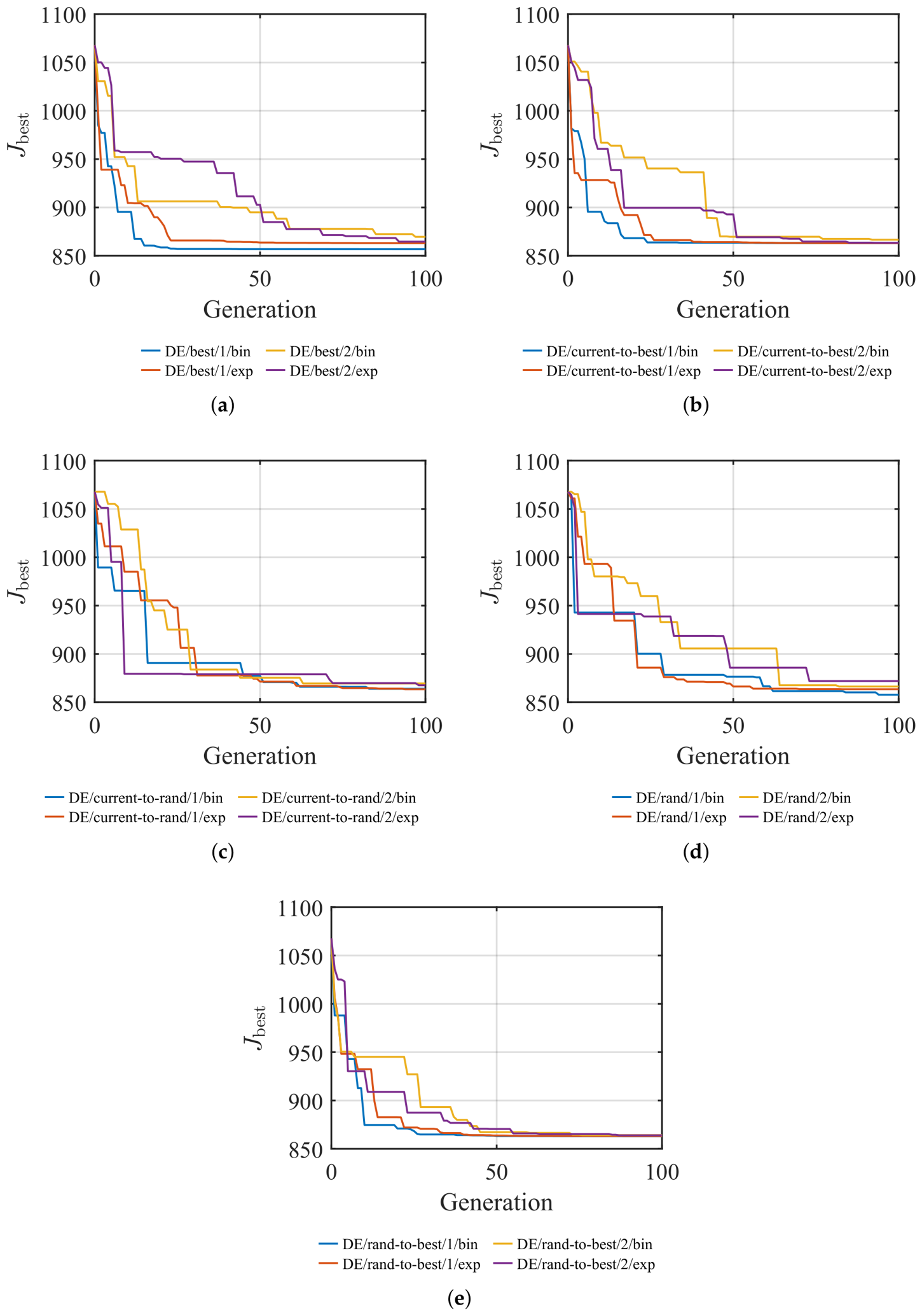
The optimization performance of the DE variants in Region 2 is analyzed through their convergence speed. Figure 5a–e illustrate the evolution of the best objective-function value ( J Best ) over successive generations for all variants, grouped by mutation strategy.
As shown in Figure 5a,b,e, exploitation-oriented variants based on best, current-to-best, and rand-to-best mutation strategies with a single differentiation exhibit faster convergence, with  J Best stabilizing within a smaller number of generations. This behavior is mainly due to the stronger exploitation tendency characteristic of these variants. Here, new candidate solutions are produced around high-performing individuals, which confines the search to a more limited region of the solution space.
In contrast, exploration-oriented variants, particularly those based on rand-type strategies and/or two differentiations, tend to converge more slowly, as shown in Figure 5c,d. This slower convergence is associated with increased population diversity and a wider search region. Nevertheless, after a sufficient number of generations, the performance differences between exploration- and exploitation-based strategies become less pronounced, and further improvements in J Best appear increasingly influenced by stochastic effects rather than by the mutation strategy alone.
The optimization results are summarized in Table 5, which presents the optimized controller parameters and the corresponding objective-function values obtained for each DE variant under the Region 2 configuration described in Section 5.
According to Table 5, the DE/best/1/bin variant attains the lowest objective value among the evaluated strategies, reaching 856.8178 at generation 94. However, this result does not imply slow convergence. By generation 25, the objective value has already decreased to 856.9840, indicating that the variant approaches a near-optimal solution within relatively few generations, followed by only marginal refinements. The final improvement amounts to only 0.1662 units (approximately 0.02%), which is consistent with the convergence behavior observed in Figure 5a.
Although DE/best/1/bin achieves the lowest objective value, a comparable value of 857.7840 at generation 94 is also reached by the DE/rand/1/bin variant. The main difference lies in the convergence dynamics, as this variant exhibits a slower rate of improvement, as shown in Figure 5d. For instance, at generation 93, the objective value is 860.267, whereas at generation 25 it remains at 900.2380, representing a reduction of 42.4540 units (4.44%). The remaining variants exhibit convergence patterns consistent with their respective mutation strategies, as previously discussed.

6.1.2. Closed-Loop Controller Performance in Region 2

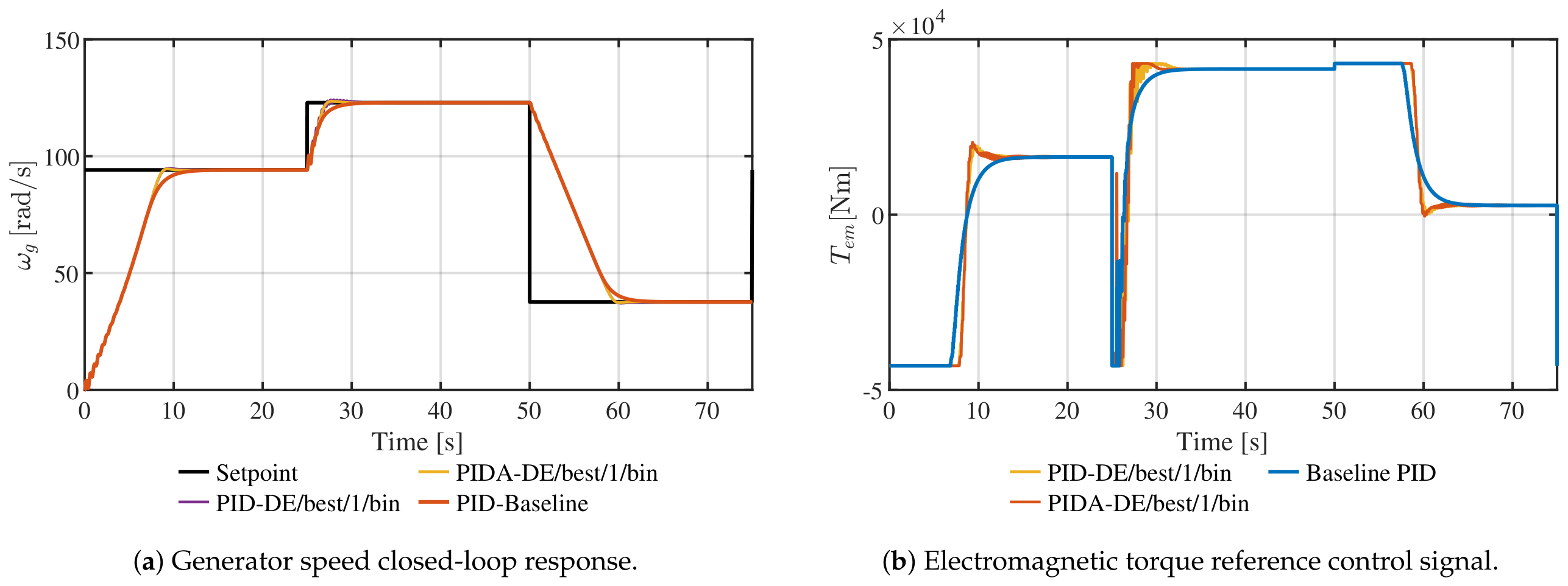
The closed-loop dynamic response of the system and the corresponding control actions are shown in Figure 6a,b. The controllers considered in this analysis are the PIDA controller tuned using the DE variant that achieved the lowest objective-function value under the Region 2 fixed-seed configuration reported in Table 5, a PID controller tuned using the same variant, and a PID controller tuned using the MATLAB PID Tuner, which serves as the baseline for performance comparison. The corresponding controller parameters used in this comparison are summarized in Table 6.
Controller performance is quantitatively assessed using transient-response characteristics together with the integral performance index (IAE) associated with the cost function in this operative region. Owing to the nonlinear dynamics of the system and the presence of multiple reference changes, transient metrics vary across transitions. Therefore, overshoot and settling time are reported for each setpoint change defined in Section 5.1 and illustrated in Figure 6a. These metrics, along with the IAE index, are summarized in Table 7.
As indicated in Table 7, several PIDA controllers achieve slightly lower IAE values than the PID controller tuned with DE/best/1/bin, while all evaluated DE-tuned controllers yield lower IAE values than the baseline controller under the considered Region 2 scenario. In particular, the PIDA controller tuned with DE/best/1/bin achieves a 0.2% improvement over the PID tuned with the same variant according to the IAE criterion, which is used as the cost function in Region 2, and a 2.93% improvement relative to the baseline controller.
Nevertheless, these controllers exhibit noticeable differences in their transient response characteristics. In general, the baseline controller presents no overshoot, indicating a more damped response; however, this also results in slower dynamics. This behavior is reflected in the settling times, where the baseline controller consistently shows larger values for all setpoint changes. In contrast, PIDA-DE/best/1/bin exhibits a slight advantage over PID-DE/best/1/bin in terms of overshoot, while maintaining very similar settling times.
The limited performance gap between the PID and PIDA controllers in Region 2 can be attributed to the low-order, quasi-linear behavior dominating this operating regime. As discussed in Section 2.4, the electrical generator is modeled as a first-order linear system and acts as the dominant actuator in Region 2. Under these conditions, the additional acceleration action of the PIDA controller does not yield systematic performance improvements, and a well-tuned PID controller can achieve comparable closed-loop behavior.
This interpretation is consistent with the control signals shown in Figure 6b, where the DE-tuned PID exhibits a more aggressive control action, accelerating convergence toward the reference while maintaining a transient response comparable to that of the PIDA controller.
Finally, under the considered Region 2 scenario, the baseline controller yields a higher IAE value than all evaluated DE-tuned controllers. This difference is consistent with the fact that the DE-based approach directly optimizes controller parameters on the nonlinear model under the Region 2 operating conditions, whereas the baseline controller is obtained using MATLAB PID Tuner. Overall, these results support the effectiveness of the proposed DE-based tuning framework for the evaluated Region 2 configuration.

6.2. Region 3 Results

6.2.1. Optimization Performance of DE Variants in Region 3

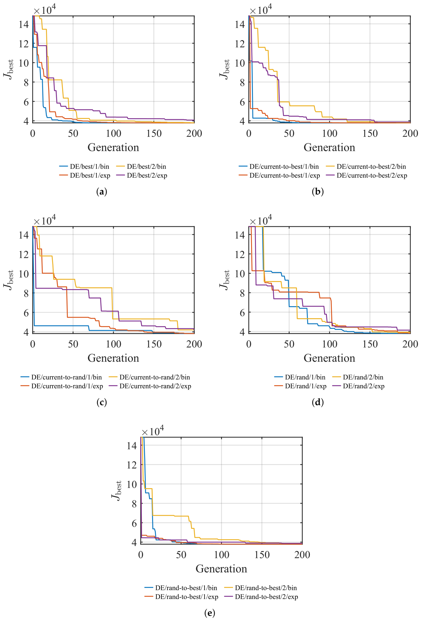
Region 3 is analyzed following the same methodology adopted for Region 2, with particular emphasis on convergence speed under a more demanding and nonlinear operating regime. Figure 7a–e illustrate the evolution of the best objective value ( J Best ) over successive generations for all DE variants, grouped according to their mutation strategy.
Compared to Region 2, the convergence behavior observed in Region 3 exhibits more pronounced differences among the evaluated DE variants. As shown in Figure 7a,b,e, variants based on best-individual mutation strategies combined with a single differentiation order tend to converge more rapidly, reaching stable objective values within a smaller number of generations.
This behavior reflects a stronger emphasis on exploitation, whereby the search process remains concentrated around the best-performing individuals, limiting large parameter variations and promoting faster convergence under the considered operating conditions.
In contrast, the convergence curves shown in Figure 7c,d indicate that exploration-oriented variants generally exhibit slower convergence. In Region 3, this effect is more pronounced than in Region 2, which can be attributed to the increased nonlinearity and sensitivity of the optimization landscape. The broader exploration induced by these variants leads to larger parameter perturbations, which in some cases result in poorer objective values and less consistent convergence behavior, thereby delaying convergence.
The optimization results are summarized in Table 8, which reports the optimized parameter vectors and corresponding objective values obtained for each DE variant under the parameters defined in Section 5. All variants were tuned using the PIDA controller structure.
Under the considered Region 3 fixed-seed configuration, the DE/best/1/bin variant achieves the lowest recorded objective-function value, reaching 37,840.68 at generation 184. Similar to Region 2, this variant exhibits only minor improvements in the cost function during later generations. In fact, at generation 91, the objective value is 37,849.00, indicating that before reaching half of the total generations, the solution is already close to its final value, with a difference of 8.32 units (approximately 0.02%).
In contrast to Region 2, two additional variants achieve objective-function values very close to the lowest recorded value. The first is DE/current-to-best/1/bin, reaching 37,840.70 at generation 188. Similar to DE/best/1/bin, this variant exhibits only minor improvements in later generations, reaching 37,847.10 at generation 103, which corresponds to an improvement of approximately 0.02%. The second variant is DE/rand-to-best/1/bin, reaching an objective value of 37,840.96 at generation 191. As in the previous cases, the improvement after generation 119 is approximately 0.02%.
In this region, the three variants with the lowest recorded objective-function values also exhibit comparable convergence speeds. These variants are based on mutation strategies that use the best individual. For the considered Region 3 scenario, the results suggest that an appropriate balance between exploration and exploitation is important for convergence behavior. The remaining variants exhibit convergence patterns consistent with their respective mutation strategies, as previously discussed.

6.2.2. Closed-Loop Controller Performance in Region 3

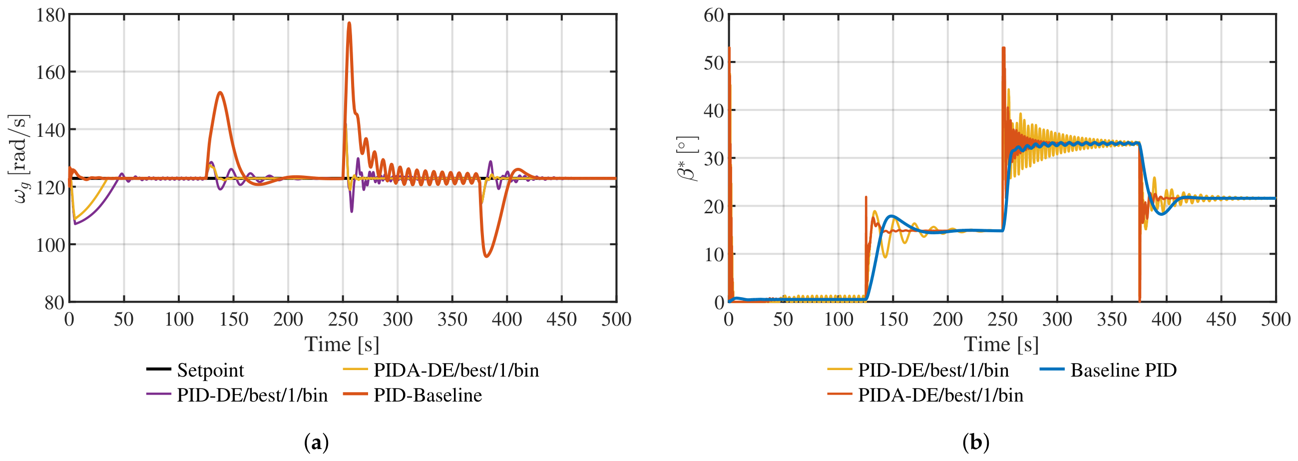
Figure 8a,b show the system responses and corresponding control signals under Region 3 operating conditions. The results are presented for the PID and PIDA controllers tuned using DE/best/1/bin, which achieved the lowest objective-function value under the Region 3 fixed-seed configuration reported in Table 8, together with a PID controller tuned using the MATLAB PID Tuner, which serves as the baseline. The corresponding controller parameters used in this comparison are summarized in Table 9.
The system response in Region 3 is quantified using integral performance indices. Unlike Region 2, classical transient-response metrics are not considered, as the primary control objective is disturbance rejection rather than reference tracking. In this operating region, metrics such as overshoot and settling time are largely influenced by the disturbance magnitude rather than by the intrinsic system dynamics. Accordingly, only integral performance indices are reported in Table 9.
As shown in Table 9, the PIDA controller outperforms the PID controller in Region 3, in contrast to the behavior observed in Region 2. Using DE/best/1/bin, which yielded the lowest objective-function value under the considered Region 3 configuration, the PIDA controller achieves an improvement of approximately 64% in the ITAE criterion—used as the cost function in Region 3—relative to the PID controller tuned with the same DE variant, and about 92% compared with the baseline controller.
This marked performance gain is attributed to the increased dynamic complexity of Region 3, where the blade pitch angle becomes the dominant control input. According to Equations (1)–(3), the pitch angle directly influences the dominant nonlinear aerodynamic component of the system. Under these conditions, the system exhibits higher-order and strongly nonlinear dynamics, which justify the use of a more complex control structure. The additional zeros introduced by the acceleration action of the PIDA controller enable more effective compensation of nonlinearities, as reflected in Figure 8b, where the PIDA controller exhibits faster and less oscillatory control actions than the PID.
As in Region 2, the evaluated DE-tuned controllers yield lower objective-function values than the baseline under the considered Region 3 scenario; however, the performance gap is more pronounced in this region. This can be attributed to the fact that the DE-based framework directly optimizes the controller gains on the nonlinear model under the defined Region 3 operating conditions, which is reflected in lower ITAE values under the evaluated disturbance-rejection scenario.
These results support the suitability of the proposed DE-based tuning framework for the considered Region 3 configuration.

6.3. Validation Under Real Wind Profile

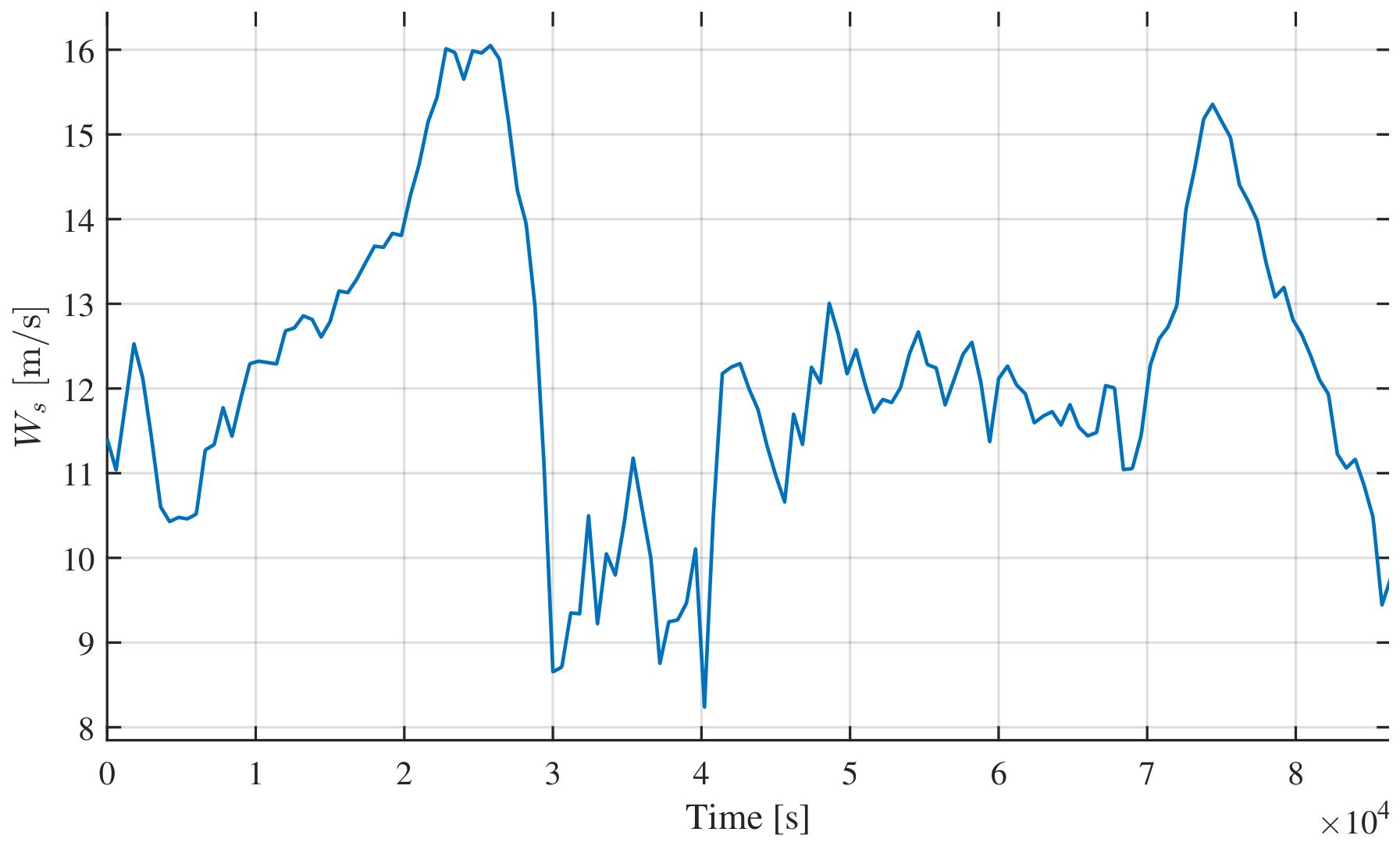
To validate the controllers obtained in Section 6.1.2 and Section 6.2.2, a real wind-speed profile measured by a Supervisory Control and Data Acquisition (SCADA) system from a wind turbine was used [43]. Specifically, the wind profile recorded on 7 January 2018, shown in Figure 9, was selected.
Both the baseline controller and the selected DE-tuned controllers were evaluated using the wind profile shown in Figure 9, which spans wind-speed ranges suitable for analyzing transitions between operating regions.
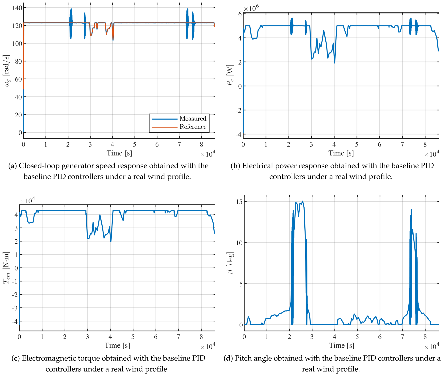
The generator angular speed and its reference, obtained with the baseline controllers, are shown in Figure 10a.
Although the controlled variable is the generator speed, the most relevant output for power production is the active electrical power, defined by Equation (9) and shown in Figure 10b.
The control signals corresponding to Figure 10a,b are shown in Figure 10c,d. As observed in Figure 10c, the electromagnetic torque presents a smoother behavior than the pitch angle shown in Figure 10d. In contrast, the pitch signal exhibits more pronounced oscillations, which are transferred to the generator-speed response and contribute to the oscillatory behavior observed in Figure 10a.
As discussed in Section 6.2, the baseline PID controller in Region 3 exhibits a relatively slow dynamic response. Consequently, the control action tends to oscillate in an attempt to compensate for wind-induced speed deviations and recover the rated operating condition. This behavior not only increases the oscillatory content of the system output, but also has a physical implication for the turbine. Repeated pitch variations may increase the activity and wear of the pitch actuator, while oscillations in generator speed may introduce additional mechanical stress in the drivetrain and rotor shaft. Therefore, the analysis of the control signals confirms that the baseline PID controller does not only present poorer numerical performance, but also a less desirable dynamic behavior from an operational and mechanical perspective.
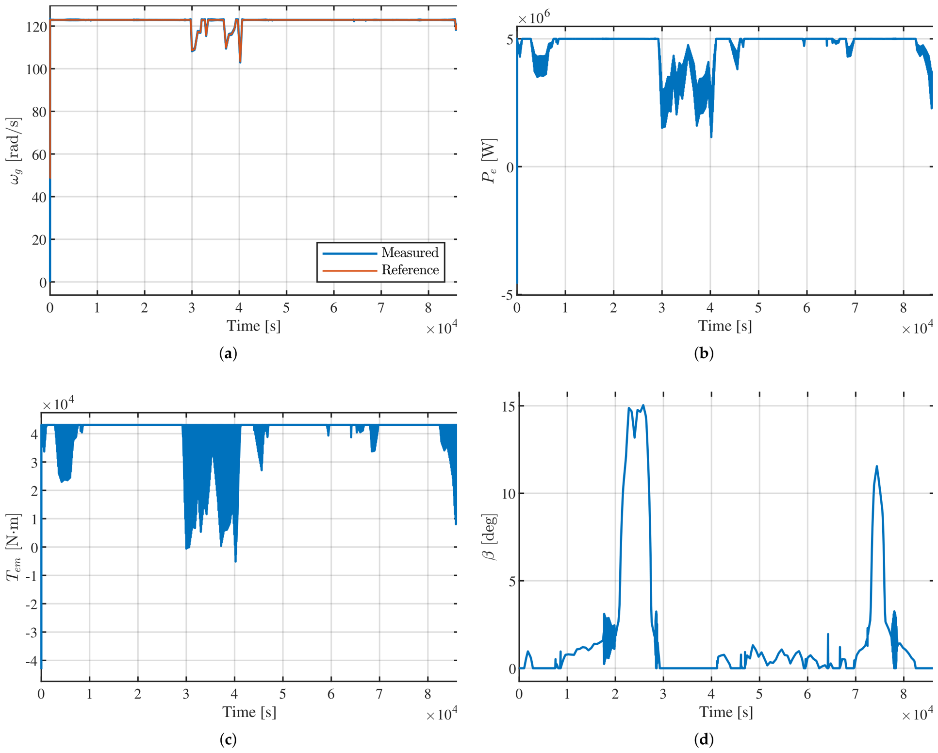
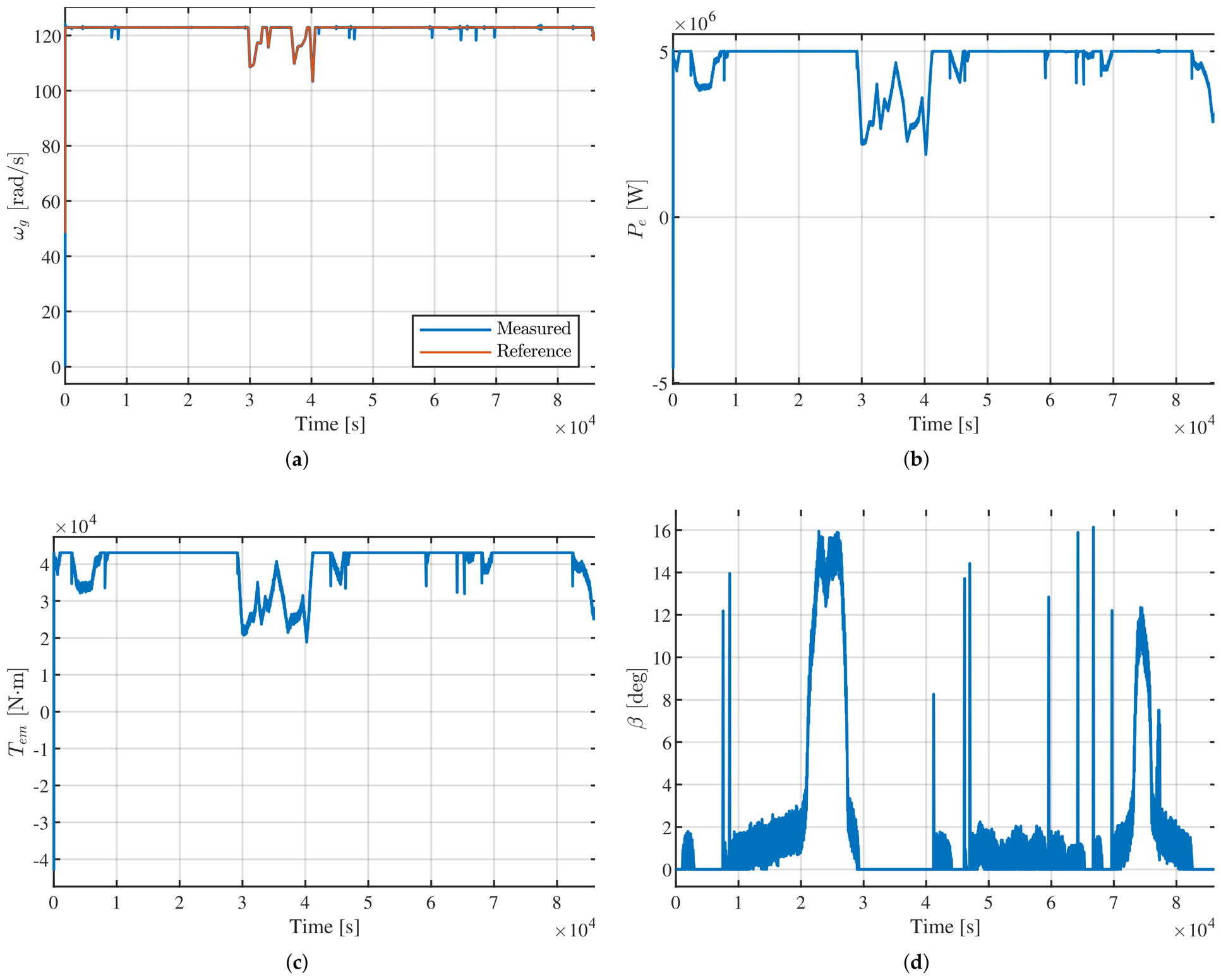
The same evaluation scenario was subsequently applied using the PIDA-DE/best/1/bin controller in Region 2 and the PIDA-DE/best/1/bin controller in Region 3. The resulting generator angular speed is shown in Figure 11a. It is worth noting that the reference signals computed by the MPPT strategy exhibit slight variations depending on the selected controller, as they are influenced by internal model variables.
Figure 11a reveals a noteworthy behavior. Under high-load operating conditions, the controller tuned for Region 3 outperforms the baseline controller. This improvement is also reflected in the pitch-angle signal shown in Figure 11d, which is clearly smoother than the corresponding signal obtained with the baseline PID controller.
Although the DE-tuned PIDA controller shows a clear improvement in Region 3, its performance is comparatively less favorable in Region 2. In this operating region, the generator-speed response exhibits small oscillations, particularly around 0.5 × 10 4 s and during the interval between 3 × 10 4 s and 4 × 10 4 s .
This response suggests a highly oscillatory control behavior in Region 2, with a consequent degradation in the quality of the control action. The corresponding electromagnetic torque control effort is shown in Figure 11c. As observed, the control signal exhibits repeated oscillatory corrections under this operating condition, which are then reflected in the generator-speed response shown in Figure 11a. From a physical perspective, this behavior is undesirable because persistent oscillatory control actions may increase dynamic loading on the drivetrain and rotor shaft.
In accordance with Equation (9), the active electrical power also exhibits oscillatory behavior in Region 2, as shown in Figure 11b. This response is not favorable for power generation, since fluctuations in generator speed and electromagnetic torque are directly reflected in the generated electrical power. From an operational perspective, these power variations may lead to undesirable fluctuations in the power injected into the grid, potentially affecting power quality if not properly mitigated. Therefore, although the DE-tuned PIDA controller improves the response in Region 3, its behavior in Region 2 indicates poorer generalization under real wind conditions.
The observed performance degradation in Region 2 can be further interpreted by analyzing Table 5. Two controllers are particularly noteworthy: DE/best/1/bin, which achieved the lowest J value under the considered Region 2 configuration, and the closely following DE/rand/1/bin. These controllers are of special interest because their gain values differ significantly from those of the remaining controllers, which tend to cluster around a similar local minimum of the objective function J.
To quantify whether the final controller configuration preserves its performance beyond the tuning scenarios, the performance indices were normalized with respect to their corresponding baseline values. For the tuning scenarios, the Region 2 PID-DE IAE and the Region 3 PIDA-DE ITAE were divided by the respective baseline values, yielding normalized ratios of 0.9727 and 0.0772 . These values were combined using their geometric mean, as shown in Equation (15).
C tune = 0.9727 × 0.0772 = 0.2739 .
The same normalization was applied to the SCADA validation results using the IAE and ITAE values reported in Table 10. The resulting normalized ratios were 0.0326 and 0.0185 , respectively, and their geometric mean is given by Equation (16).
C SCADA = 0.0326 × 0.0185 = 0.0246 .
The composite generalization gap is defined as the difference between the SCADA and tuning indicators. Using Equations (15) and (16), the resulting value is given by Equation (17).
G = C SCADA C tune = 0.2494 .
The negative value of G indicates that the relative performance of the final controller configuration does not deteriorate under the independent SCADA wind profile. Instead, its normalized performance relative to the baseline improves during validation, supporting the generalization capability of the selected PID controller in Region 2 and PIDA controller in Region 3.
This behavior may indicate a degree of overfitting to the optimization scenario. This behavior is consistent with their strong performance under the tuning conditions. In particular, the best performance is obtained with DE/best/1/bin. However, their performance degrades when they are evaluated under operating conditions different from those used during tuning.
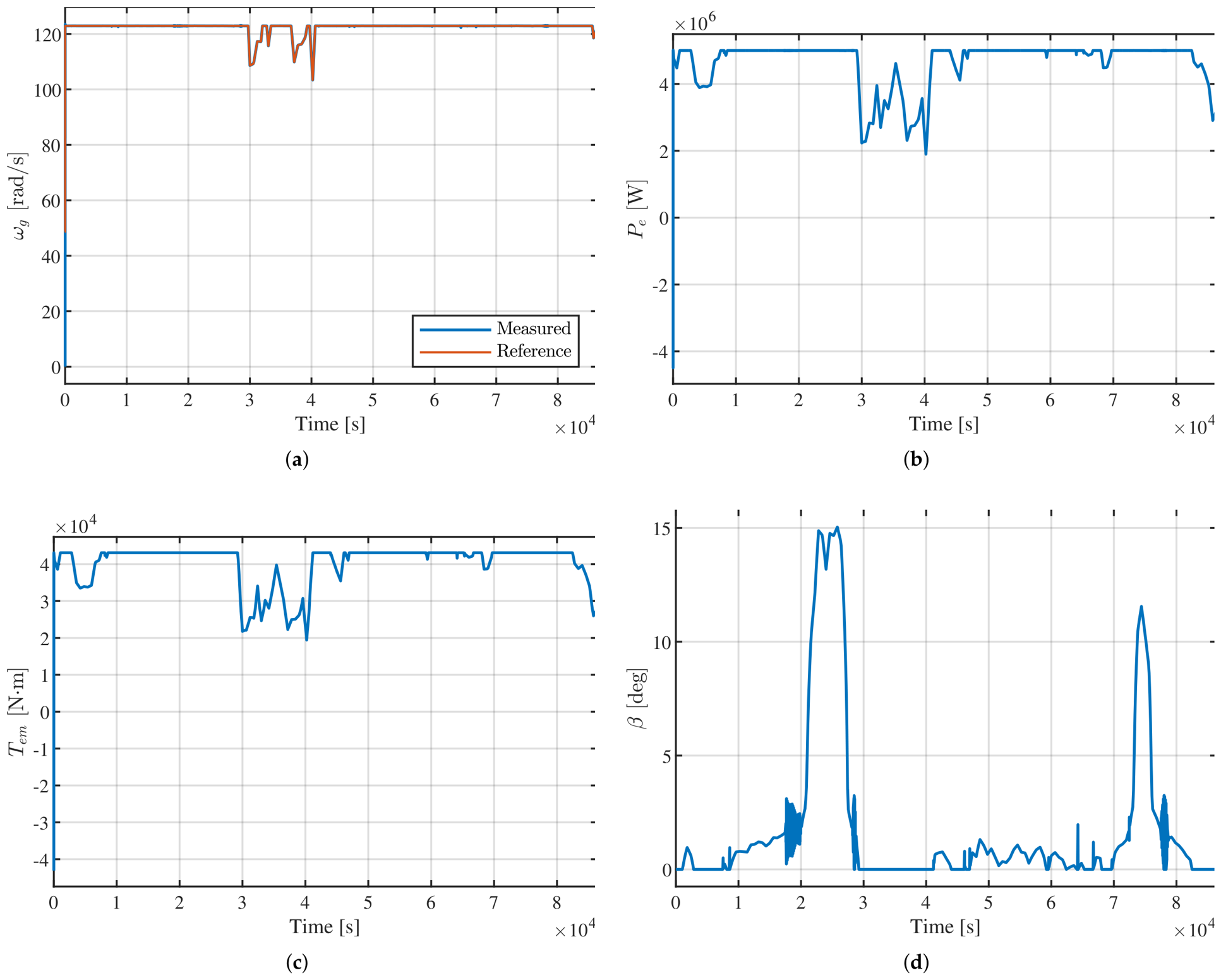
Given this scenario, it becomes necessary to select a controller that avoids the previously observed signs of overfitting. According to Table 5, among the PIDA controllers that did not exhibit these signs, DE/rand-to-best/1/bin achieved the lowest objective-function value, with J = 863.06 . However, as shown in Table 6, the PID controller tuned using DE/best/1/bin achieves a lower value of J = 858.60 , outperforming the PIDA controllers that maintained satisfactory generalization behavior under the measured wind profile. Therefore, the PID controller is selected for operation in Region 2, while the DE-tuned PIDA controller selected for Region 3 is retained for above-rated operation. The generator-speed response and electrical-power output obtained with this combined control strategy are presented in Figure 12a and Figure 12b, respectively. The corresponding electromagnetic-torque and pitch-angle signals obtained with the selected DE-tuned controllers are shown in Figure 12c and Figure 12d, respectively. Compared with the previous cases, both control signals exhibit noticeably smoother behavior, which contributes to reducing the oscillations observed in the generator-speed and active-power responses.
With this combination of controllers, both Region 2 and Region 3 outperform the baseline controller, achieving improved reference tracking with reduced error. These results can be quantitatively assessed using integral performance indices, whose values are reported in Table 10.
With the appropriate selection of controllers, the performance evaluated using real data corresponding to a full day of operation shows a significant improvement for the DE-based controllers. Specifically, these controllers achieve reductions of 96.7%, 95.8%, 98.1%, and 99.9% in the IAE, ISE, ITAE, and ITSE indices, respectively.
These results show that the benefits of the optimal DE-tuned controllers are not limited to improved tracking performance. The smoother control signals also contribute to a more stable active-power response and may reduce unnecessary mechanical stress on the drivetrain and pitch actuators. This highlights the importance of appropriate controller tuning in wind turbine applications, demonstrating that performance does not depend solely on using more complex controller structures, but also on selecting gain parameters that produce a balanced dynamic response.
In contrast to the results obtained under tuning conditions, the most suitable option for the partial-load region under a real wind profile, with the MPPT strategy active, is a well-tuned PID controller, owing to the relative simplicity of the system dynamics in this operating regime. On the other hand, Region 3 presents more complex dynamics, as discussed in Section 6.2.2, where the PIDA architecture offers a clear advantage over the classical PID controller.
Accurate control of the generator angular speed results in a more stable active power output, since electrical power depends directly on generator speed. Accordingly, the active power dynamics closely follow those of the generator speed, as shown in Figure 10b, Figure 11b and Figure 12b, highlighting the role of precise speed regulation in ensuring stable power generation under real operating conditions.
It should be noted that negative electrical power values appear during the initial transient, as the turbine temporarily draws energy from the grid to overcome inertial effects and initiate drivetrain rotation.

6.4. Robustness Evaluation Under Combined Non-Ideal Conditions

To complement the nominal validation based on the measured wind-speed profile, an additional robustness stress test was performed under a combined set of non-ideal operating conditions. The controller parameters obtained during the original DE tuning process were kept unchanged, such that the test evaluates the sensitivity of the previously tuned controllers rather than performing a new optimization.
A simultaneous parametric perturbation was introduced into the wind turbine model. The turbine and generator inertias were increased by 10%, the drivetrain stiffness and damping were reduced by 10%, and the natural frequency and damping ratio of the pitch actuator were reduced by 10%. In addition, the generator time constant was increased by 10% to represent a slower generator response.
Measurement uncertainty was introduced into the generator-speed feedback signal using a Band-Limited White Noise block with a noise power of 10 5 and a sampling time of 0.1 s. The block default seed value of 23341 was retained to ensure reproducibility of the noise realization. The resulting measurement was processed by a first-order low-pass filter with a time constant of 0.5 s before being supplied to the controller. The same measured wind-speed profile employed in the nominal validation was retained so that changes in performance could be attributed to the introduced non-idealities rather than to variations in the wind excitation.
This combined scenario is not intended to represent a mathematically determined worst-case condition, but rather a deliberately challenging robustness stress test designed to assess whether the performance advantages observed under nominal simulation conditions are preserved when simultaneous model uncertainty and measurement disturbances are introduced.
The closed-loop responses obtained under the combined robustness stress-test scenario are shown in Figure 13, while the corresponding integral performance indices are summarized in Table 11. Despite the simultaneous introduction of parameter uncertainty and measurement disturbances, the closed-loop responses remained bounded throughout the complete real wind profile, although increased tracking deviations and control activity were observed relative to the nominal SCADA-based validation.
As expected, these non-ideal conditions degraded the performance of the DE-tuned control strategy. The IAE increased from 795.00 to 4147.00, corresponding to a 421.64% increase, while the ISE increased by 80.54%, from 8676.00 to 15,663.48. Greater relative increases were observed in the time-weighted indices, with the ITAE increasing by 739.85% and the ITSE by 11,361.47%.
The particularly large increase in ITSE indicates that persistent tracking deviations occurring at later stages of the wind profile are strongly penalized by the time-weighted squared-error formulation. Therefore, this increase should not be interpreted independently as an equivalent deterioration in the physical response of the turbine. In contrast, the considerably smaller increase in ISE indicates that the overall accumulated squared tracking error remains substantially less affected than suggested by the time-weighted metric.
Despite this degradation, the closed-loop response remained bounded throughout the complete measured wind-speed profile, demonstrating that the controller maintained stable operation under the simultaneous introduction of plant-parameter variations and noisy measurements. These results indicate that the performance gains obtained during nominal optimization are sensitive to non-ideal operating conditions, particularly when persistent errors are emphasized, while also showing that the DE-tuned controller retains closed-loop regulation capability without retuning.


7. Conclusions

The results obtained under the considered experimental scenarios indicate that the DE-tuned controllers outperform the MATLAB PID Tuner baseline controllers across the evaluated performance indices. This advantage is particularly pronounced in Region 3, where the stronger nonlinear aerodynamic dynamics and the disturbance-rejection requirements make controller tuning more demanding. Under these conditions, the additional degrees of freedom provided by the PIDA structure result in a substantial performance improvement over the conventional PID controller. In Region 2, however, the performance difference between PID and PIDA structures is considerably smaller, and the subsequent evaluation under a measured wind profile indicates that a well-tuned PID controller provides a more suitable response. These findings indicate that controller performance depends not only on the selected architecture, but also on its compatibility with the dynamic characteristics and control objectives of each wind turbine operating region.
The results also show that the controller achieving the lowest objective-function value under the tuning conditions is not necessarily the most suitable when evaluated under a different wind scenario. In Region 2, some controllers that achieved favorable tuning-stage results exhibited oscillatory behavior when subsequently evaluated in simulation using a measured SCADA wind-speed profile, indicating reduced generalization performance and signs of overfitting. This observation highlights the importance of evaluating tuned controllers beyond the specific scenario used during optimization. Consequently, controller selection should not rely exclusively on the objective-function value obtained during tuning, but should also consider the dynamic response under operating conditions that differ from those used in the optimization process.
A central methodological contribution of this work is the adoption of a controlled and reproducible benchmarking protocol for comparing classical DE variants. Although Differential Evolution is inherently stochastic, the use of a fixed random seed, a predefined random-number generator, common initial populations, and consistent simulation conditions within each operating region enables the reported optimization experiments to be reproduced under the same computational environment. This procedure reduces initialization- and implementation-related inconsistencies and provides a common experimental basis for examining differences in convergence behavior and resulting controller performance. Nevertheless, the reported results correspond to the considered fixed-seed stochastic realization and operating scenarios and should therefore be interpreted as a reproducible within-scenario comparison rather than as a statistical characterization of the DE variants across independent random realizations.
The proposed framework provides a structured basis that can be extended to other controller architectures, optimization variants, and nonlinear control problems following the same experimental methodology. Its current implementation, however, relies on an accurate mathematical representation of the controlled system because the complete tuning and validation process is performed in simulation. Furthermore, validation using measured wind-speed data does not reproduce all effects associated with physical wind turbine operation, such as measurement noise, communication delays, parameter uncertainty, actuator nonlinearities, or unmodeled dynamics. These aspects represent important limitations when considering direct implementation in real systems.
Future work should therefore extend the framework toward Hardware-in-the-Loop (HIL) and real-time simulation environments, where implementation-specific effects that are not reproduced in the present continuous-time simulation can be explicitly evaluated. These include finite sampling periods, computational and communication delays, sampling jitter, numerical precision limitations, and synchronization between sensing, control computation, and actuation, in addition to measurement noise, parameter uncertainty, and nonlinear actuator behavior. These timing-related effects may be particularly relevant for the PIDA architecture because its derivative and acceleration actions can be more sensitive to phase lag, irregular sampling, and high-frequency disturbances. It should be emphasized that Differential Evolution is used only during the offline tuning stage; therefore, the real-time computational requirements are associated with the implementation of the resulting fixed-parameter controller rather than with the optimization algorithm itself.
The primary objective of this work was not to establish a statistically significant ranking among the evaluated DE variants, but rather to develop a reproducible benchmarking framework in which controller structure, objective function, initialization, population size, stopping criteria, and simulation conditions are consistently defined across all variants. Within this framework, the fixed-seed strategy was adopted to isolate algorithmic differences under a common and fully reproducible initialization. As a natural extension, the proposed framework can be used with multiple independent random seeds and statistical analyses to quantify performance variability and assess the consistency of the observed DE-variant rankings across stochastic realizations. The same framework can also be extended toward multi-objective optimization, including criteria such as control effort, actuator activity, and electrical power performance, thereby broadening its applicability to more comprehensive controller benchmarking studies.

Author Contributions

Study conception and design, A.G.U.R., N.D.V. and J.C.Z.A.; data collection, A.G.U.R. and N.D.V.; software A.G.U.R. and N.D.V.; Methodology, A.G.U.R. and N.D.V.; analysis and interpretation of results, A.G.U.R., N.D.V. and J.C.Z.A.; writing—original draft preparation, A.G.U.R. and N.D.V.; writing—review and editing, J.C.Z.A. All authors have read and agreed to the published version of the manuscript.

Funding

This work was supported by Universidad Politécnica Salesiana through the research project “Bio-inspired optimization for the design of controllers oriented to energy efficiency in engineering systems,” under Project Resolution No. 002-001-2026-02-02.

Institutional Review Board Statement

Not applicable.

Informed Consent Statement

Not applicable.

Data Availability Statement

The complete MATLAB/Simulink implementation of the proposed benchmarking framework, including the controller-tuning scripts and wind turbine models used in this study, is publicly available as a versioned software release archived in Zenodo (version 1.0.0, DOI: 10.5281/zenodo.21832106). The measured wind-speed data used for the SCADA-based validation are available from the dataset cited in Ref. [43].

Acknowledgments

The authors used ChatGPT, based on OpenAI’s GPT-5.5 model, to assist with language refinement of the manuscript, optimization of MATLAB code, and generation of the images included within the Simulink subsystems of the proposed model in Figure 4. All AI-assisted content was carefully reviewed and verified by the authors to ensure its accuracy, consistency, and correctness. The authors approved all AI-assisted contributions and take full responsibility for the final content of the work.

Conflicts of Interest

The authors declare no conflicts of interest.

References

  1. Åström, K.J.; Murray, R.M. Feedback Systems: An Introduction for Scientists and Engineers; Princeton University Press: Princeton, NJ, USA, 2008; pp. 27–64. [Google Scholar]
  2. Slotine, J.J.E.; Li, W. Applied Nonlinear Control; Prentice Hall: Englewood Cliffs, NJ, USA, 1991; Volume 199. [Google Scholar]
  3. Abdelbaky, M.A.; Liu, X.; Kong, X. Wind turbines pitch controller using constrained fuzzy-receding horizon control. In Proceedings of the 2019 Chinese Control And Decision Conference (CCDC), Nanchang, China, 3–5 June 2019; IEEE: Piscataway, NJ, USA, 2019; pp. 236–241. [Google Scholar]
  4. Hwas, A.; Katebi, R. Wind turbine control using PI pitch angle controller. IFAC Proc. Vol. 2012, 45, 241–246. [Google Scholar] [CrossRef] [Scilit]
  5. Wang, T. A brief review on wind turbine aerodynamics. Theor. Appl. Mech. Lett. 2012, 2, 062001. [Google Scholar] [CrossRef] [Scilit]
  6. Dai, J.; Liu, D.; Wen, L.; Long, X. Research on power coefficient of wind turbines based on SCADA data. Renew. Energy 2016, 86, 206–215. [Google Scholar] [CrossRef] [Scilit]
  7. Kandil, A. Study of Hopf curves in the time delayed active control of a 2DOF nonlinear dynamical system. SN Appl. Sci. 2020, 2, 1924. [Google Scholar] [CrossRef] [Scilit]
  8. Kandil, A.; Eissa, M. Improvement of positive position feedback controller for suppressing compressor blade oscillations. Nonlinear Dyn. 2017, 90, 1727–1753. [Google Scholar] [CrossRef] [Scilit]
  9. Wang, J.; Golnary, F.; Li, S.; Weerasuriya, A.U.; Tse, K.T. A review on power control of wind turbines with the perspective of dynamic load mitigation. Ocean Eng. 2024, 311, 118806. [Google Scholar] [CrossRef] [Scilit]
  10. Kong, X.; Ma, L.; Liu, X.; Abdelbaky, M.A.; Wu, Q. Wind turbine control using nonlinear economic model predictive control over all operating regions. Energies 2020, 13, 184. [Google Scholar] [CrossRef] [Scilit]
  11. Astrom, K.J.; Hägglund, T. Advanced PID control. IEEE Control Syst. 2006, 26, 98–101. [Google Scholar] [CrossRef]
  12. Jung, S.; Dorf, R.C. Analytic PIDA controller design technique for a third order system. In Proceedings of the 35th IEEE Conference on Decision and Control, Kobe, Japan, 11–13 December 1996; IEEE: Piscataway, NJ, USA, 1996; Volume 3, pp. 2513–2518. [Google Scholar]
  13. Huba, M.; Bistak, P.; Vrancic, D. Parametrization and Optimal Tuning of Constrained Series PIDA Controller for IPDT Models. Mathematics 2023, 11, 4229. [Google Scholar] [CrossRef] [Scilit]
  14. Hu, X.; Tan, W.; Hou, G. Tuning of PID/PIDD2 Controllers for Second-Order Oscillatory Systems with Time Delays. Electronics 2023, 12, 3168. [Google Scholar] [CrossRef] [Scilit]
  15. Wright, A.D. Advanced Control Design for Wind Turbines; Part I: Control Design, Implementation, and Initial Tests; Technical Report NREL/TP-500-42437; National Renewable Energy Laboratory: Golden, CO, USA, 2008. [Google Scholar] [CrossRef] [Scilit]
  16. Campregher, F.; Milanesi, M.; Schiavo, M.; Visioli, A. Generalized Haalman Tuning of PIDA Controllers. IFAC-PapersOnLine 2024, 58, 406–411. [Google Scholar] [CrossRef] [Scilit]
  17. Huba, M.; Bisták, P.; Brieznik, J.; Vrančić, D. Constrained Series PI, PID and PIDA Controller Design. Power Electron. Drives 2024, 9, 331–346. [Google Scholar] [CrossRef] [Scilit]
  18. Huba, M.; Bisták, P.; Vrančić, D. Series PIDA Controller Design for IPDT Processes. Appl. Sci. 2023, 13, 2040. [Google Scholar] [CrossRef] [Scilit]
  19. Milanesi, M.; Mirandola, E.; Visioli, A. A comparison between PID and PIDA controllers. In Proceedings of the 27th IEEE International Conference on Emerging Technologies and Factory Automation, ETFA, Stuttgart, Germany, 6–9 September 2022; Institute of Electrical and Electronics Engineers Inc.: Piscataway, NJ, USA, 2022; pp. 1–6. [Google Scholar] [CrossRef] [Scilit]
  20. Nawikavatan, A.; Puangdownreong, D. Optimal PIDA Controller Design for Truck Breaking System using Flower Pollination Algorithm. In Proceedings of the 2019 7th International Electrical Engineering Congress (iEECON); IEEE: Piscataway, NJ, USA, 2019; pp. 1–4. [Google Scholar]
  21. Mosaad, A.M.; Attia, M.A.; Abdelaziz, A.Y. Whale optimization algorithm to tune PID and PIDA controllers on AVR system. Ain Shams Eng. J. 2019, 10, 755–767. [Google Scholar] [CrossRef] [Scilit]
  22. Mousakazemi, S.M.H.; Ayoobian, N. Robust tuned PID controller with PSO based on two-point kinetic model and adaptive disturbance rejection for a PWR-type reactor. Prog. Nucl. Energy 2019, 111, 183–194. [Google Scholar] [CrossRef] [Scilit]
  23. Zambrano, J.; Carpio, M. Intelligent tuning of PID controllers: Comprehensive approach based on modified Particle Swarm Optimization (PSO) algorithm. In Proceedings of the IECON Proceedings (Industrial Electronics Conference), Chicago, IL, USA, 3–6 November 2024; IEEE Computer Society: Piscataway, NJ, USA, 2024; pp. 1–6. [Google Scholar] [CrossRef] [Scilit]
  24. Feng, H.; Ma, W.; Yin, C.; Cao, D. Trajectory control of electro-hydraulic position servo system using improved PSO-PID controller. Autom. Constr. 2021, 127, 103722. [Google Scholar] [CrossRef] [Scilit]
  25. Storn, R.; Price, K. Differential Evolution—A Simple and Efficient Heuristic for Global Optimization over Continuous Spaces. J. Glob. Optim. 1997, 11, 341–359. [Google Scholar] [CrossRef] [Scilit]
  26. Kaliappan, P.; Ilangovan, A.; Muthusamy, S.; Sembanan, B. Temperature Control Design with Differential Evolution Based Improved Adaptive-Fuzzy-PID Techniques. Intell. Autom. Soft Comput. 2023, 36, 781–801. [Google Scholar] [CrossRef] [Scilit]
  27. Gün, A. Attitude control of a quadrotor using PID controller based on differential evolution algorithm. Expert Syst. Appl. 2023, 229, 120518. [Google Scholar] [CrossRef] [Scilit]
  28. Saad, M.S.; Jamaluddin, H.; Darus, I.Z.M. Implementation of PID controller tuning using differential evolution and genetic algorithms. Int. J. Innov. Comput. Inf. Control 2012, 8, 7761–7779. [Google Scholar]
  29. Mezura-Montes, E.; Velázquez-Reyes, J.; Coello Coello, C.A. A comparative study of differential evolution variants for global optimization. In Proceedings of the 8th Annual Conference on Genetic and Evolutionary Computation, Seattle, WA, USA, 8–12 July 2006; Association for Computing Machinery: New York, NY, USA, 2006; pp. 485–492. [Google Scholar] [CrossRef] [Scilit]
  30. Jeyakumar, G.; Shanmugavelayutham, C. Convergence Analysis of Differential Evolution Variants on Unconstrained Global Optimization Functions. Int. J. Artif. Intell. Appl. 2011, 2, 116–127. [Google Scholar] [CrossRef] [Scilit]
  31. Jeyakumar, G.; Velayutham, C.S. A Comparative Performance Analysis of Multiple Trial Vectors Differential Evolution and Classical Differential Evolution Variants. In Proceedings of the Rough Sets, Fuzzy Sets, Data Mining and Granular Computing, Delhi, India, 16–18 December 2009; Kumar, C.M., Ella, H.A., Ślezak, D., Hiroshi, S., Eds.; Springer: Berlin/Heidelberg, Germany, 2009; pp. 470–477. [Google Scholar]
  32. Chakraborty, S.; Saha, A.K.; Sharma, S.; Sahoo, S.K.; Pal, G. Comparative Performance Analysis of Differential Evolution Variants on Engineering Design Problems. J. Bionic Eng. 2022, 19, 1140–1160. [Google Scholar] [CrossRef] [Scilit] [PubMed]
  33. Georgioudakis, M.; Plevris, V. A Comparative Study of Differential Evolution Variants in Constrained Structural Optimization. Front. Built Environ. 2020, 6, 102. [Google Scholar] [CrossRef] [Scilit]
  34. Brest, J.; Maučec, M.S. Comparative Study of Modern Differential Evolution Algorithms: Perspectives on Mechanisms and Performance. Mathematics 2025, 13, 1556. [Google Scholar] [CrossRef] [Scilit]
  35. Das, S.; Suganthan, P.N. Differential evolution: A survey of the state-of-the-art. IEEE Trans. Evol. Comput. 2011, 15, 4–31. [Google Scholar] [CrossRef] [Scilit]
  36. Hellwig, M.; Beyer, H.G. Benchmarking evolutionary algorithms for single objective real-valued constrained optimization—A critical review. Swarm Evol. Comput. 2019, 44, 927–944. [Google Scholar] [CrossRef] [Scilit]
  37. Almufti, S.; Asaad, R.; Shaban, A.; Marqas, R. Benchmarking metaheuristic algorithms: A comprehensive review of test functions, real-world problems, and evaluation metrics. J. Electron. Netw. Appl. Math. 2025, 5, 16–35. [Google Scholar] [CrossRef] [Scilit]
  38. Bartz-Beielstein, T.; Doerr, C.; Berg, D.v.d.; Bossek, J.; Chandrasekaran, S.; Eftimov, T.; Fischbach, A.; Kerschke, P.; La Cava, W.; Lopez-Ibanez, M.; et al. Benchmarking in optimization: Best practice and open issues. arXiv 2020, arXiv:2007.03488. [Google Scholar]
  39. Jonkman, J.; Butterfield, S.; Musial, W.; Scott, G. Definition of a 5-MW Reference Wind Turbine for Offshore System Development; Technical Report; National Renewable Energy Laboratory: Golden, CO, USA, 2009.
  40. Heier, S. Grid Integration of Wind Energy Conversion Systems; Wiley: Hoboken, NJ, USA, 1998. [Google Scholar]
  41. Visioli, A. Practical PID Control; Springer: Berlin/Heidelberg, Germany, 2006. [Google Scholar]
  42. Urgilés Rojas, A.G.; Dueñas Vargas, N. DE-Tuning Framework for Wind Turbine Controllers in MATLAB R2024b, version 1.0.0; Zenodo: Geneva, Switzerland, 2026. [Google Scholar] [CrossRef]
  43. Erisen, B. Wind Turbine SCADA Dataset. Kaggle. 2018. Available online: https://www.kaggle.com/datasets/berkerisen/wind-turbine-scada-dataset (accessed on 1 August 2025).
Figure 1. Wind turbine system control block diagram.
Energies 19 04420 g001
Figure 2. Power curve and operating regions of the NREL 5-MW wind turbine.
Energies 19 04420 g002
Figure 3. Block diagram of the PIDA controller structure.
Energies 19 04420 g003
Figure 4. Simulink block diagram of the nonlinear wind turbine model and control structure.
Energies 19 04420 g004
Figure 5. Convergence curves of the DE variants in Region 2, grouped according to their mutation strategies: (a) best; (b) current-to-best; (c) current-to-rand; (d) rand; and (e) rand-to-best.
Energies 19 04420 g005
Figure 6. Closed-loop performance in Region 2: (a) generator speed response; (b) electromagnetic torque reference control signal.
Energies 19 04420 g006
Figure 7. Convergence curves of the DE variants in Region 3, grouped according to their mutation strategies: (a) best; (b) current-to-best; (c) current-to-rand; (d) rand; and (e) rand-to-best.
Energies 19 04420 g007
Figure 8. Closed-loop performance in Region 3: (a) generator speed closed-loop response; (b) pitch angle reference control signal.
Energies 19 04420 g008
Figure 9. Measured wind-speed profile recorded by a SCADA system on 7 January 2018, at an operational wind turbine located in Turkey, used for real wind validation of the tuned controllers.
Energies 19 04420 g009
Figure 10. Closed-loop responses obtained with the baseline PID controllers under a real wind profile: (a) generator speed response; (b) electrical power response; (c) electromagnetic torque; and (d) pitch angle.
Energies 19 04420 g010
Figure 11. Closed-loop responses obtained using DE-tuned PIDA controllers under a real wind profile: (a) generator speed response in Regions 2 and 3; (b) electrical power response in Regions 2 and 3; (c) electromagnetic torque reference in Region 2; and (d) pitch angle in Regions 2 and 3.
Energies 19 04420 g011
Figure 12. Closed-loop responses obtained using the optimal DE-tuned controllers under a real wind profile: (a) generator speed response in Regions 2 and 3; (b) electrical power response in Regions 2 and 3; (c) electromagnetic torque reference in Region 2; and (d) pitch angle in Regions 2 and 3.
Energies 19 04420 g012
Figure 13. Closed-loop responses obtained using the optimal DE-tuned controllers under the combined robustness stress-test scenario, including parametric uncertainty and measurement noise, with a real wind profile: (a) generator speed response in Regions 2 and 3; (b) electrical power response in Regions 2 and 3; (c) electromagnetic torque reference in Region 2; and (d) pitch angle in Regions 2 and 3.
Energies 19 04420 g013
Table 1. Definition of signals associated with the wind turbine system.
SymbolNameDescriptionUnits
vWind speedIncoming wind velocity acting on the rotorm/s
ω g Generator speed referenceDesired generator angular speedrad/s
β Pitch angle referenceReference signal for the pitch actuatordeg
τ e m Electromagnetic torque referenceReference torque command for the electric generatorN·m
β Pitch angleActual blade pitch angle applied to the pitch actuatordeg
τ t Aerodynamic torqueTorque produced by aerodynamic forces on the rotorN·m
ω t Turbine speedAngular speed of the turbine rotorrad/s
τ e m Electromagnetic torqueTorque generated by the electric generatorN·m
ω g Generator speedAngular speed of the generator shaftrad/s
P e Electrical powerElectrical power delivered by the generatorW
Table 2. Technical Specifications of the NREL 5-MW Reference Wind Turbine [39].
ParameterSymbolUnitValue
Rated electrical power P e kW5000
Rated generator torque τ e m N·m43,093.55
Rotor cut-in and rated speeds ω r rpm6.9, 12.1
Cut-in, rated, and cut-out wind speeds v c i , v r a t , v c o m/s3, 11.6, 25
Shaft stiffness K s N·m/rad 8.67637 × 10 8
Shaft damping D s N·m/(rad/s) 6.215 × 10 6
Generator inertia J g kg·m2534.116
Rotor inertia J t kg·m2 3.8768 × 10 7
Blade radiusrm63
Number of blades3
Generator torque actuator time constant τ g s0.1
Pitch actuator natural frequency ω n rad/s0.88
Pitch actuator damping ratio ζ 0.1
Generator efficiency η 94.4%
Gearbox ratio N g 97
Pitch angle range β min , β max deg0, 90
Maximum pitch rate β ˙ max deg/s8
Table 3. Classical DE variants considered in this study, compiled by the authors according to the standard Differential Evolution nomenclature [25].
BestCurrent-to-BestCurrent-to-RandRandRand-to-Best
DE/best/1/binDE/current-to-best/1/binDE/current-to-rand/1/binDE/rand/1/binDE/rand-to-best/1/bin
DE/best/1/expDE/current-to-best/1/expDE/current-to-rand/1/expDE/rand/1/expDE/rand-to-best/1/exp
DE/best/2/binDE/current-to-best/2/binDE/current-to-rand/2/binDE/rand/2/binDE/rand-to-best/2/bin
DE/best/2/expDE/current-to-best/2/expDE/current-to-rand/2/expDE/rand/2/expDE/rand-to-best/2/exp
Table 4. DE algorithm parameters for Regions 2 and 3.
ParameterRegion 2Region 3
N p 5060
N g 100200
F0.950.75
C r 0.850.65
Table 5. Controller parameters obtained for Region 2 using the evaluated DE variants.
DE Variants K p K i K d K a t d t a J
DE/best/1/bin−21,980.67−29,227.26−1272.37−2323.730.00001.0000856.8178
DE/best/1/exp−11,226.71−11,410.84−663.64−570.261.00001.0000863.0720
DE/best/2/bin−12,229.69−18,183.97−1328.99−839.590.68160.8426869.5981
DE/best/2/exp−11,304.46−11,625.60−1179.54−329.341.00000.9421864.6257
DE/current-to-best/1/bin−11,228.99−11,475.11−665.80−564.511.00000.9981863.0799
DE/current-to-best/1/exp−11,229.42−11,225.36−604.28−622.061.00001.0000863.0677
DE/current-to-best/2/bin−13,811.77−18,742.50−1197.17−1005.371.00000.9562866.6106
DE/current-to-best/2/exp−11,396.95−11,229.76−538.75−737.491.00001.0000863.4415
DE/current-to-rand/1/bin−11,695.05−12,602.65−939.81−949.181.00000.9981864.0145
DE/current-to-rand/1/exp−11,465.74−12,416.15−660.27−770.371.00001.0000863.4790
DE/current-to-rand/2/bin−11,841.71−19,480.26−2595.26−416.701.00000.6800869.4631
DE/current-to-rand/2/exp−11,634.84−17,691.50−1213.18−988.411.00000.9538867.6122
DE/rand-to-best/1/bin−11,229.18−11,253.08−618.60−603.300.99990.9998863.0618
DE/rand-to-best/1/exp−11,222.11−11,432.91−682.65−552.071.00000.9993863.0779
DE/rand-to-best/2/bin−12,343.11−12,055.43−783.80−609.221.00001.0000864.1299
DE/rand-to-best/2/exp−11,759.62−12,280.18−927.91−515.681.00001.0000863.9362
DE/rand/1/bin−20,672.59−27,865.40−1323.54−2920.820.00001.0000857.7840
DE/rand/1/exp−10,814.06−9865.85−450.15−706.831.00001.0000863.5519
DE/rand/2/bin−19,910.04−40,000.00−548.90−5695.060.00001.0000866.2967
DE/rand/2/exp−12,231.34−19,689.97−443.28−2515.021.00001.0000871.8872
Table 6. Controller parameters considered for the comparative analysis in Region 2.
Controller K p K i K d K a t d t a J
PIDA-DE/best/1/bin−21,980.67−29,227.26−1272.37−2323.730.00001.0000856.82
PID-DE/best/1/bin−12,580.80−13,770.95−907.571.0000858.60
PID-baseline−10,801.54−5677.39−439.400.0045882.72
Table 7. Transient response and IAE performance for the evaluated controllers in Region 2.
Controller M p 1 [%] T s 1 [s] M p 2 [%] T s 2 [s] M p 3 [%] T s 3 [s] IAE
PID-baseline0.000010.1790.00002.93220.000011.690882.72
PID-DE/best/1/bin0.790988.55004.28661.90000.623439.5000858.60
PIDA-DE/best/1/bin0.472098.50002.20351.85000.342869.4500856.82
PIDA-DE/best/1/exp0.906798.60005.00502.15000.698509.5000863.07
PIDA-DE/best/2/bin2.02929.350010.5714.15001.540310.750869.60
PIDA-DE/best/2/exp1.04838.60005.32222.15000.816859.5000864.63
PIDA-DE/current-to-best/1/bin0.921068.60005.07662.15000.709629.5000863.08
PIDA-DE/current-to-best/1/exp0.848038.60004.84472.15000.648709.5500863.07
PIDA-DE/current-to-best/2/bin1.29388.50008.95003.60000.9841510.400866.61
PIDA-DE/current-to-best/2/exp0.754548.60004.89292.15000.574269.5500863.44
PIDA-DE/current-to-rand/1/bin1.12958.55005.98912.10000.858929.4500864.01
PIDA-DE/current-to-rand/1/exp1.05388.55006.00522.10000.804909.4500863.48
PIDA-DE/current-to-rand/2/bin2.44239.700010.4893.85001.876910.900869.46
PIDA-DE/current-to-rand/2/exp2.15069.500010.2403.50001.637110.800867.61
PIDA-DE/rand-to-best/1/bin0.856448.60004.86282.15000.655929.5500863.06
PIDA-DE/rand-to-best/1/exp0.917478.60005.01342.15000.707549.5000863.08
PIDA-DE/rand-to-best/2/bin0.542108.65005.13932.40000.423469.6000864.13
PIDA-DE/rand-to-best/2/exp0.914358.60005.57742.10000.704899.5000863.94
PIDA-DE/rand/1/bin0.759408.50003.48061.85000.552419.4000857.78
PIDA-DE/rand/1/exp0.657298.65003.82012.15000.504799.6000863.55
PIDA-DE/rand/2/bin1.72148.40009.93343.15001.269610.300866.30
PIDA-DE/rand/2/exp2.18829.450011.7204.40001.634210.700871.89
Table 8. Controller parameters obtained for Region 3 using the evaluated DE variants.
DE Variants K p K i K d K a t d t a J
DE/best/1/bin−1.540−0.4800−1.461−2.5201.200.293437,840.68
DE/best/1/exp−1.538−0.4794−1.457−2.5151.200.293337,842.58
DE/best/2/bin−1.507−0.4861−1.428−2.4251.110.289737,959.76
DE/best/2/exp−1.754−0.5054−2.847−3.0441.660.261340,747.20
DE/current-to-best/1/bin−1.541−0.4804−1.462−2.5231.200.293337,840.70
DE/current-to-best/1/exp−1.537−0.4784−1.446−2.5181.200.294337,842.66
DE/current-to-best/2/bin−1.416−0.4660−1.842−2.5201.580.297438,212.42
DE/current-to-best/2/exp−1.418−0.4980−1.882−2.5721.690.307538,764.24
DE/current-to-rand/1/bin−1.621−0.4826−1.598−2.5851.280.282838,289.70
DE/current-to-rand/1/exp−1.519−0.4488−1.406−2.4911.390.294038,231.59
DE/current-to-rand/2/bin−2.028−0.5224−1.673−2.8060.7600.249242,014.17
DE/current-to-rand/2/exp−0.978−0.5532−5.000−2.7623.000.301841,852.01
DE/rand-to-best/1/bin−1.544−0.4793−1.448−2.5211.200.293437,840.96
DE/rand-to-best/1/exp−1.545−0.4804−1.466−2.5261.210.293237,841.34
DE/rand-to-best/2/bin−1.566−0.4108−0.936−2.3240.8560.292738,690.03
DE/rand-to-best/2/exp−1.485−0.4263−1.702−2.6081.780.303338,723.54
DE/rand/1/bin−1.552−0.4708−1.427−2.5091.200.296537,913.82
DE/rand/1/exp−1.516−0.4895−1.784−2.6751.610.298938,166.10
DE/rand/2/bin−1.190−0.5290−2.907−2.6742.210.304439,310.77
DE/rand/2/exp−1.619−0.4320−3.572−2.9112.930.286641,438.06
Table 9. Controller parameters considered for the comparative analysis in Region 3.
Controller K p K i K d K a t d t a J
PIDA-DE/best/1/bin−1.5397−0.4800−1.4614−2.52001.20330.293437,840.68
PID-DE/best/1/bin−0.3795−0.6547−1.97200.0000103,995.39
PID-baseline−0.21607−0.0274330.622883.6336490,439.68
Table 10. Integral performance indices comparison between baseline and DE-tuned controllers.
Controller IAE ISE ITAE ITSE
Baseline controllers24,369.22208,961.821,197,181,581.249,932,493,251.26
Best DE controllers795.008676.0022,155,416.562,610,996.73
Table 11. Performance degradation of the selected DE-tuned control strategy under the combined robustness stress-test scenario.
IndexNominalPerturbedDegradation (%)
IAE795.004147.00421.64
ISE8676.0015,663.4880.54
ITAE22,155,416.56186,071,665.88739.85
ITSE2,610,996.73299,258,604.9711,361.47
Disclaimer/Publisher’s Note: The statements, opinions and data contained in all publications are solely those of the individual author(s) and contributor(s) and not of MDPI and/or the editor(s). MDPI and/or the editor(s) disclaim responsibility for any injury to people or property resulting from any ideas, methods, instructions or products referred to in the content.