A Study of Myopic, Predictive, and Reinforcement Learning Energy Management Strategies for Isolated Microgrids

Abstract

The increasing penetration of renewable energy sources in isolated microgrids has intensified the need for Energy Management Systems (EMS) capable of reducing diesel dependence while ensuring reliable operation. This study compares three EMS strategies for a photovoltaic–diesel–battery microgrid representative of remote communities in the Brazilian Amazon: a Myopic strategy (M1), a Predictive strategy (M2), and a PPO-RL strategy (M3), evaluated under identical physical and operational constraints using real irradiance and demand data over the complete year of 2025 at a 15 min resolution. The three strategies achieved very similar diesel consumption, with a difference of less than 0.7% between the best and worst cases; M2 achieved the lowest consumption (218,863.19 L), the highest renewable penetration (52.14%), and the lowest curtailment (1.06%), with M3 performing comparably but with more frequent generator starts. An illustrative, qualitative analysis of the highest- and lowest-PV days suggested that differences among strategies become more pronounced under high photovoltaic availability, while low renewable availability drives all strategies toward similar diesel-dominated operation. These findings indicate that the main benefit of advanced EMS strategies lies not in large diesel savings, but in improved coordination and utilization of renewable and storage resources. Additionally, a simplified economic analysis of the photovoltaic–battery hybridization, based on M2’s diesel savings, showed an internal rate of return of approximately 30.7% p.a. and a payback period of approximately 3.2 years, well above the 14% p.a. benchmark, confirming the hybridization as an economically attractive investment regardless of which EMS strategy is adopted.

1. Introduction

The growing demand for electricity in remote and geographically isolated regions has intensified the development of isolated microgrids as an alternative to conventional centralized power systems [1]. In many of these regions, especially in isolated communities of the Brazilian Amazon, electricity generation remains strongly dependent on diesel generators, resulting in elevated operational costs, fuel transportation difficulties, reduced energy efficiency, and significant environmental impacts associated with greenhouse gas emissions [2,3]. Additionally, the operational performance of these systems is strongly influenced by fuel quality and combustion efficiency, motivating the development of advanced monitoring and management solutions in remote locations [4,5].

Microgrids are decentralized energy systems composed of distributed generation sources, energy storage systems, controllable loads, and dispatchable generation units capable of operating either connected to the utility grid or in islanded mode [6,7,8]. In isolated applications, the integration of Photovoltaic Generation (PV) with Battery Energy Storage Systems (BESS) has emerged as one of the main strategies for reducing diesel dependence, increasing renewable energy penetration, improving operational flexibility, and mitigating power fluctuations [9,10]. However, the intermittent and uncertain nature of solar generation introduces important challenges related to energy balance, operational stability, and dynamic coordination among microgrid assets. Under these conditions, the overall system performance becomes strongly dependent on the capability of the EMS to efficiently coordinate renewable generation, battery utilization, and diesel generator dispatch under highly variable operating conditions [11,12].

Several EMS approaches have been proposed in the literature and can generally be categorized into optimization-based, predictive, and data-driven methods. Traditional optimization-based strategies, such as rule-based and myopic approaches, determine operating actions based exclusively on the instantaneous state of the system, frequently limiting the exploitation of the temporal flexibility provided by energy storage systems [13]. To overcome this limitation, predictive strategies, particularly Model Predictive Control (MPC), have been widely investigated due to their capability to incorporate forecasts of renewable generation and load demand into the decision-making process [14,15]. By considering future operating conditions over a finite prediction horizon, predictive EMS approaches can improve battery coordination and reduce diesel consumption [16].

Reinforcement learning (RL) and deep reinforcement learning (DRL) have increasingly been investigated as alternatives to conventional optimization-based energy management strategies for microgrids, particularly because they can learn control policies directly from interactions with the operating environment. Lei et al. [17] proposed a deep reinforcement learning approach for dynamic energy dispatch in isolated microgrids, demonstrating the potential of DRL to adapt energy dispatch decisions to changing renewable generation and load conditions. Similarly, Bao and Xu [18] developed a data-driven energy management strategy based on DRL for microgrid systems, highlighting the ability of learning-based approaches to derive operational policies without explicitly solving an optimization problem at every time step. These studies indicate that RL is particularly relevant when the operating environment is dynamic and characterized by uncertainties that are difficult to represent explicitly in conventional optimization formulations.

The flexibility of RL has also motivated its application to more complex microgrid coordination problems. Harrold et al. [19] investigated multi-agent deep reinforcement learning for renewable energy integration and energy trading, illustrating how multiple learning agents can coordinate distributed energy resources and energy exchanges. More recently, Wang et al. [20] employed a Twin Delayed Deep Deterministic Policy Gradient (TD3) approach with prioritized experience replay for online energy management of a residential microgrid. The use of TD3 is particularly relevant to energy management problems involving continuous control variables, as the algorithm can directly learn continuous control actions while improving the stability of the actor–critic learning process. In addition, Rajamallaiah et al. [21] demonstrated the application of DRL to voltage regulation in a DC microgrid, showing that reinforcement learning can also be extended from high-level energy management toward lower-level operational control. Taken together, these studies demonstrate that RL can support different layers of microgrid operation, ranging from energy dispatch and EMS decisions to coordination among distributed resources and real-time control.

Among the most promising reinforcement learning algorithms, Proximal Policy Optimization (PPO) has received considerable attention due to its training stability and suitability for sequential decision-making in dynamic and continuous environments [22]. These characteristics are particularly relevant to the present EMS problem, in which photovoltaic generation, electrical demand, battery state of charge, and diesel generator operating conditions continuously evolve over time, while the battery power reference represents a continuous control action. Among alternative reinforcement learning approaches, PPO provides a suitable balance between control flexibility, training stability, and implementation complexity for the proposed framework. PPO has already demonstrated promising results in several energy-related applications, including smart grid control, battery dispatch optimization, and hybrid renewable system management [23,24]. Nevertheless, its application to isolated hybrid microgrids combining real operational data, photovoltaic forecasting, realistic diesel generator behavior, and complete annual operational analyses remains relatively limited, particularly for Brazilian isolated systems.

Although several studies have investigated optimization-based, predictive, and reinforcement learning approaches independently, there is still a lack of systematic comparison between fundamentally different EMS paradigms under identical physical configurations and operational constraints. In particular, comparisons that simultaneously consider long-term energy performance and short-term operational behavior remain limited. Annual indicators such as diesel consumption and renewable penetration may conceal important differences in battery utilization, generator start-stop behavior, and photovoltaic curtailment. Therefore, a comprehensive EMS assessment should consider both aggregated energy indicators and detailed operational behavior under different renewable availability conditions.

Motivated by these limitations, this work presents a comparative evaluation of three EMS strategies applied to an isolated photovoltaic–diesel-battery microgrid representative of the Brazilian Amazon. The evaluated approaches include: (i) a Myopic strategy based on current operating conditions, (ii) a Predictive strategy incorporating photovoltaic generation and load forecasts, and (iii) a PPO-RL strategy based on PPO. All three approaches operate over the same physical simulation framework, component models, and operational constraints, enabling a controlled comparison of their decision-making behavior. Real irradiance and load demand data are used for annual out-of-sample evaluation during 2025, while data from 2023 to 2024 are used for model development and training.

Unlike studies focused exclusively on aggregated annual indicators, the proposed evaluation combines a complete year-long assessment with detailed operational investigations during the highest and lowest photovoltaic generation days of the evaluation period. This approach enables the analysis of diesel consumption, generator operating behavior, battery utilization, photovoltaic curtailment, renewable energy penetration, and load-supply reliability, while also identifying the operational mechanisms responsible for differences among the EMS strategies.

The results show that the three strategies achieve similar annual diesel consumption, while more pronounced differences are observed in renewable energy utilization and operational behavior. The Predictive strategy achieves the best overall balance between diesel consumption, renewable penetration, photovoltaic curtailment, and generator operation, whereas the PPO-RL strategy achieves comparable aggregate energy performance through a distinct operating policy characterized by more frequent generator starts. The results further show that the differentiation among EMS strategies depends strongly on renewable availability: under high photovoltaic generation, greater energy flexibility allows the strategies to exhibit distinct battery and diesel dispatch behaviors, whereas under low photovoltaic availability, all methods converge toward a similar diesel-dominated operating mode.

2. Materials and Methods

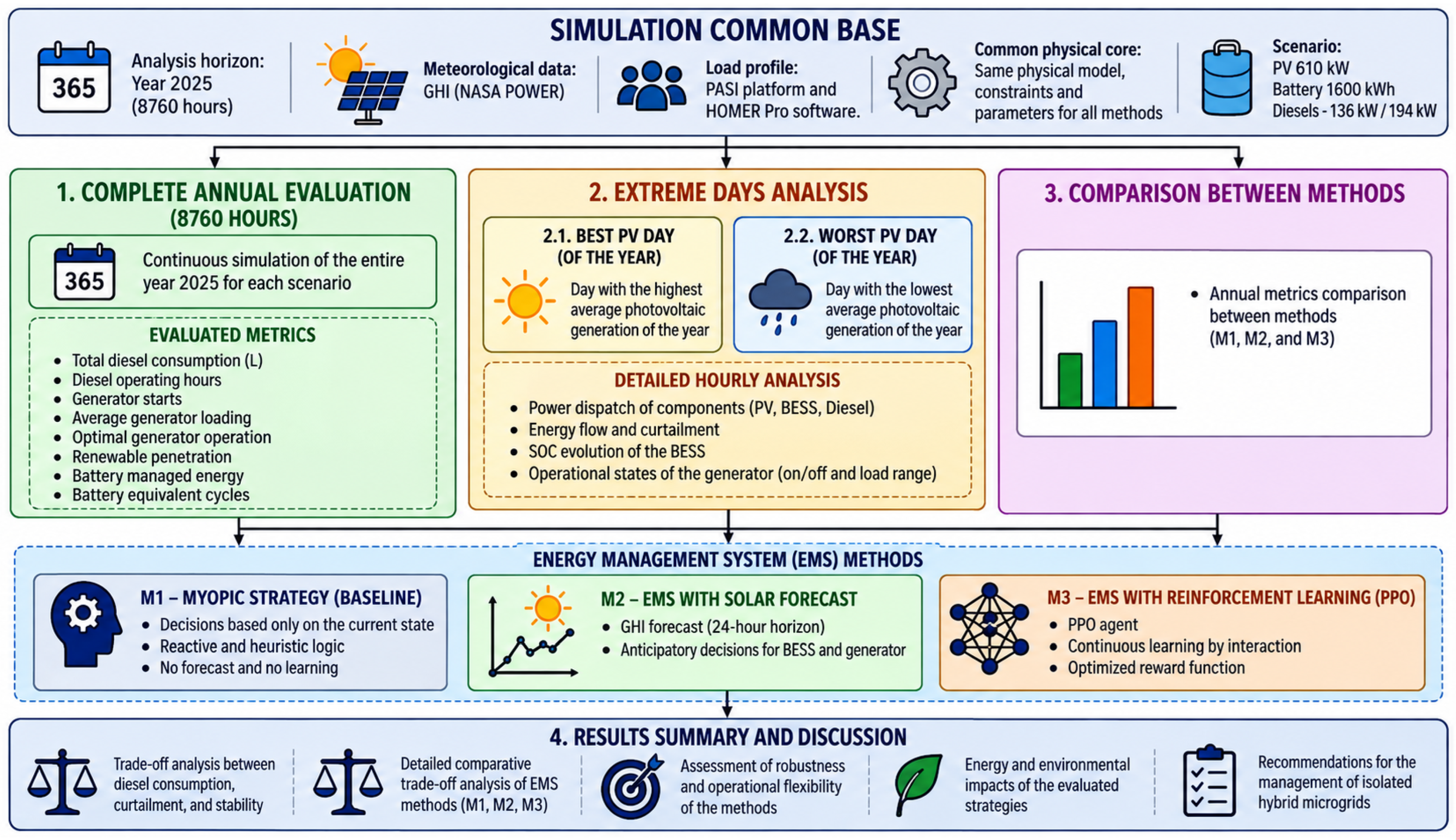
This section presents the methodological framework adopted for the development and evaluation of the proposed EMS strategies for an isolated hybrid microgrid. The methodology comprises four main stages: (i) definition of the study area and input dataset; (ii) specification of the hybrid microgrid configuration and operating scenario; (iii) implementation of the physical models and operational constraints shared by all EMS strategies; and (iv) implementation and evaluation of the three EMS approaches, denoted as M1 (Myopic strategy), M2 (Predictive strategy), and M3 (PPO-RL strategy). The overall methodological framework is illustrated in Figure 1.

2.1. Study Area and Dataset

The study considers an isolated hybrid microgrid representative of the District of Surpresa, located in the municipality of Guajará-Mirim, Rondônia State, in the Brazilian Amazon region. The locality exhibits characteristics typical of isolated electrical systems, including dependence on diesel-based generation, logistical constraints associated with fuel transportation, and the need to increase the integration of renewable energy sources.

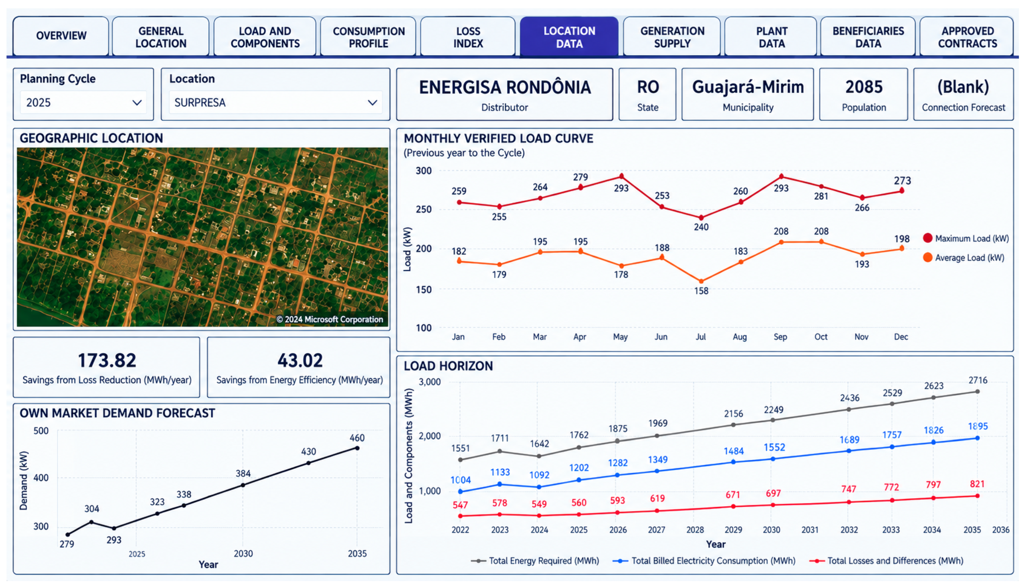
Information regarding the studied locality was obtained from the PASI/EPE platform [25], as illustrated in Figure 2.

Meteorological data were obtained from the NASA POWER platform [26], using Global Horizontal Irradiance (GHI) data for the years 2023, 2024, and 2025. Electrical demand data and preliminary information regarding the microgrid configuration were obtained from institutional EPE data available through the PASI platform and from the HOMER Pro software version 3.18 [27].

All time series were represented at a 15 min temporal resolution, resulting in 35,040 samples per year. The original hourly GHI and demand series were converted to the adopted temporal resolution through linear interpolation, with the resulting values constrained to non-negative values. The 15 min resolution was selected to provide an adequate representation of the short-term dynamics associated with photovoltaic generation, battery charging and discharging, and diesel-generator operation while maintaining computational tractability.

The datasets from 2023 to 2024 were used for model development and training, whereas 2025 was reserved exclusively for out-of-sample evaluation. This chronological separation prevents information leakage between the development and evaluation stages and enables the EMS strategies to be assessed under previously unseen operating conditions.

2.2. Microgrid Configuration and Scenario Definition

The microgrid configuration was initially defined through a techno-economic assessment using HOMER Pro. The sizing procedure targeted approximately 50% renewable penetration while maintaining at least 6 h of average battery autonomy. This approach establishes a common physical configuration for the subsequent EMS comparison, allowing differences in operational performance to be attributed primarily to the energy management strategies rather than to differences in system sizing.

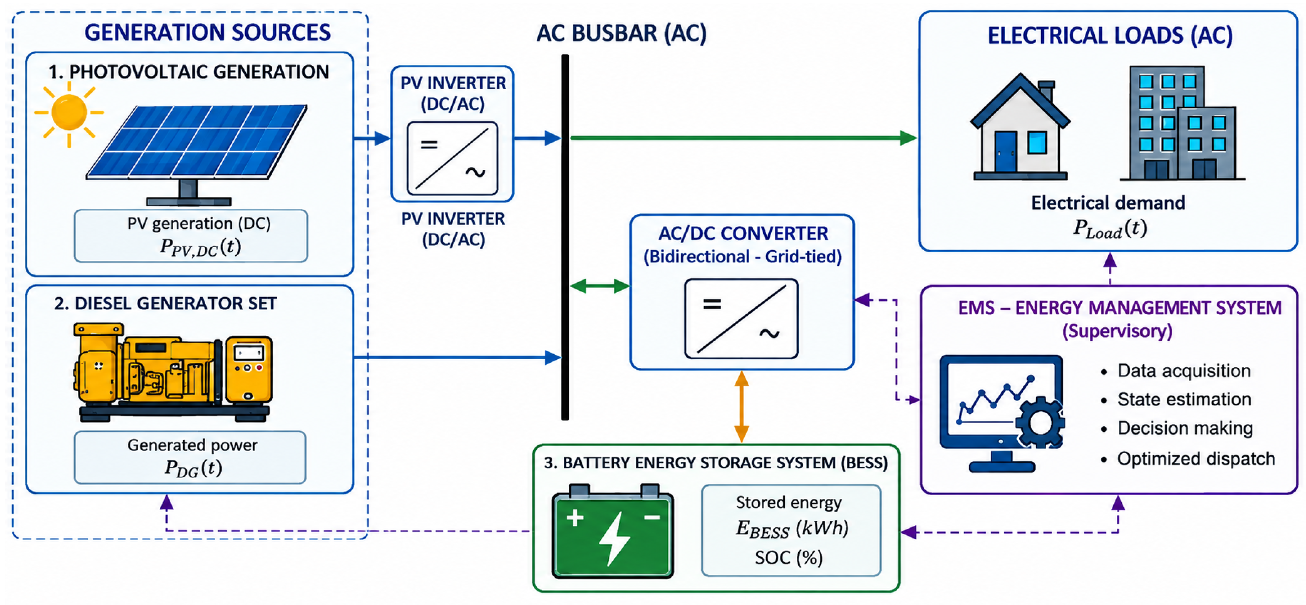
The resulting configuration comprises a 610 kW PV generation system, a 1600 kWh BESS, and a bidirectional converter with a maximum power rating of 325 kW. According to the HOMER assessment, the selected BESS provides an average autonomy of approximately 6.35 h, satisfying the minimum autonomy criterion adopted during the sizing process. The resulting hybrid microgrid configuration is illustrated in Figure 3.

The existing diesel generation infrastructure in Surpresa comprises five generator units, including two units rated at 136 kW and three units rated at 194 kW. Under the conventional operating configuration, up to three diesel generators are typically operated simultaneously to meet the electricity demand of the isolated system.

The hybridization with photovoltaic generation and battery storage reduces the diesel generation requirement during normal operation. Accordingly, the hybridized configuration evaluated in this study allows a maximum of two diesel generators to operate simultaneously. For the EMS simulations, these units are represented by one 136 kW generator and one 194 kW generator, resulting in a combined maximum diesel generation capacity of 330 kW.

The remaining units of the existing five-generator fleet are not required to operate simultaneously under the considered hybridized scenario. Instead, they remain conceptually available for generator rotation, scheduled maintenance, and contingency operation. Limiting simultaneous diesel operation to two units therefore provides greater operational flexibility for distributing operating hours and start events among the available fleet, while preserving redundancy for maintenance and critical operating conditions. This operating strategy is also consistent with the importance of continuous condition monitoring and fault detection in diesel engines, as the identification and classification of engine faults can support maintenance planning and help prevent unexpected failures [28].

The parameters adopted for the hybrid microgrid configuration are summarized in

Table 1. Parameters of the hybrid microgrid configuration evaluated in this study.

Parameter	Value
Time step (min)	15
PV nominal power (kW)	610
Performance Ratio (PR)	0.85
BESS nominal capacity (kWh)	1600
Maximum converter power (kW)	325
Charging efficiency	0.95
Discharging efficiency	0.95
Minimum SOC (%)	20
Maximum SOC (%)	95
Initial SOC (%)	50
Minimum cycle SOC (%)	30
Recharge target SOC (%)	50
Number of simultaneously dispatchable diesel units	2
Diesel unit ratings (kW)	136/194
Diesel minimum loading	30%
Minimum up time (h)	1
Minimum down time (h)	1

.

2.3. System Modeling

The hybrid microgrid is modeled as an isolated system comprising photovoltaic generation, a battery energy storage system, two simultaneously dispatchable diesel generators, and the electrical load. All EMS strategies operate over the same physical simulation layer, which is responsible for enforcing component constraints, determining the resulting power flows, updating system states, and calculating the associated operational quantities.

This common physical layer ensures that the three EMS strategies are evaluated under identical system configurations and physical constraints. Each EMS therefore determines the desired control action according to its respective methodology, while the physical layer determines the feasible system response.

2.3.1. Photovoltaic Generation Model

The photovoltaic power available to the microgrid is estimated from the GHI using a deterministic formulation:

$$P_{PV}\left(t\right)=P_{PV}^{nom}·PR·{\displaystyle \frac{GHI\left(t\right)}{1000}}$$

(1)

where $P_{PV}\left(t\right)$ is the available photovoltaic power at time step t, $P_{PV}^{nom}$ is the installed nominal PV capacity, $PR$ is the overall system performance ratio, and $GHI\left(t\right)$ is the global horizontal irradiance in W/m².

The performance ratio represents the aggregate effect of photovoltaic system losses, including temperature effects, electrical losses, conversion inefficiencies, and other system-level losses. The resulting PV power is constrained to non-negative values and limited by the installed nominal capacity.

For the selected configuration, $P_{PV}^{nom}=610$ kW and $PR=0.85$. This value was adopted based on typical performance ratios reported for well-maintained grid-connected PV systems, including installations operating under tropical climatic conditions comparable to the Brazilian Amazon, where reported PR values are commonly in the range of 0.80–0.87 [29]. The same deterministic relationship is applied throughout the simulation, ensuring consistency between the photovoltaic generation model and the EMS strategies.

Since the PR is applied as a constant scaling factor in Equation (1), it uniformly rescales the available PV power across the entire simulation horizon without altering the relative temporal profile of photovoltaic generation. Consequently, this parameter directly affects the absolute magnitude of PV generation, renewable penetration, and diesel consumption obtained for each strategy, but it does not affect the relative comparison among the EMS strategies, since $P_{PV}^{nom}$ and $PR$ are identical across M1, M2, and M3 and are applied consistently to both the forecasted and the realized PV profiles used by each method. A lower PR would proportionally reduce the available PV energy and increase the diesel and battery burden required to meet the load, while a higher PR would have the opposite effect; in both cases, the qualitative differences in operational behavior identified among the strategies, such as the more conservative battery discharge of M2 and the more frequent generator starts of M3, are expected to persist, since they stem from differences in the EMS decision logic rather than from the specific value adopted for the PR.

For Method M2, the forecasting module first predicts the future GHI values. The predicted irradiance is subsequently converted into photovoltaic power using Equation (1). Thus, the forecasting module predicts the meteorological variable directly, while the conversion from irradiance to PV power remains governed by the deterministic physical model.

2.3.2. Battery Energy Storage System Model

The BESS is modeled as the primary energy storage and flexibility component of the hybrid microgrid. The system has a nominal energy capacity of 1600 kWh and a maximum converter power of 325 kW. The charging and discharging efficiencies are both set to 95%.

The battery state-of-charge dynamics are represented by:

$$SOC(t+1)=SOC\left(t\right)+{\displaystyle \frac{{\eta }_{ch}{P}_{ch}\left(t\right)-P_{dis}\left(t\right)/{\eta }_{dis}}{E_{BESS}}}\Delta t$$

(2)

where $SOC\left(t\right)$ is the battery state of charge at time step t, $P_{ch}\left(t\right)$ and $P_{dis}\left(t\right)$ are the charging and discharging powers, respectively, ${\eta }_{ch}$ and ${\eta }_{dis}$ are the charging and discharging efficiencies, $E_{BESS}$ is the nominal battery capacity, and $\Delta t$ is the simulation time step in hours.

The physical SOC limits are defined as:

$$SO{C}_{min}\le SOC\left(t\right)\le SO{C}_{max}$$

(3)

with $SO{C}_{min}=20\%$ and $SO{C}_{max}=95\%$. The nominal initial SOC is set to 50%. During reinforcement-learning training, the initial SOC can be varied within a predefined range around this nominal value to expose the agent to different initial operating conditions.

In addition to the physical SOC limits, an operational cycle-management rule is adopted to avoid repeated deep discharge of the BESS. A SOC level of 30% is defined as the minimum preferred SOC for a discharge cycle. When this threshold is reached, further battery discharge is blocked until the battery is recharged to the target SOC of 50%. Consequently, the 20% SOC value represents the absolute physical lower boundary, whereas 30% represents the operational threshold used to terminate a discharge cycle. The 50% recharge target provides a recovery margin before a new discharge cycle is initiated.

The battery charging and discharging powers are further constrained by the maximum converter power and the available energy within the admissible SOC range. These constraints are enforced by the physical simulation layer after receiving the control request from the corresponding EMS strategy.

The selected configuration provides an average battery autonomy of approximately 6.35 h. This characteristic was one of the principal criteria adopted during system sizing, since sufficient storage autonomy enables renewable energy to be shifted across periods of reduced photovoltaic availability and can reduce unnecessary diesel-generator operation.

2.3.3. Diesel Generator Model and Operational Constraints

The diesel generation subsystem represented in the EMS consists of two simultaneously dispatchable units, rated at 136 kW and 194 kW, respectively. Each generator is modeled independently, with its own operating state, power output, operating time, start events, and fuel consumption. The maximum simultaneous diesel generation capacity represented in the simulation is therefore 330 kW.

For each generator i, the operating power is constrained according to:

$$P_{DG,i}^{min}\le P_{DG,i}\left(t\right)\le P_{DG,i}^{max}$$

(4)

when the unit is committed. The minimum operating power is defined as 30% of the nominal generator capacity. Accordingly, the minimum operating powers are 40.8 kW for the 136 kW unit and 58.2 kW for the 194 kW unit. This constraint prevents prolonged operation at excessively low loading levels and provides a more realistic representation of diesel-generator operation.

The generators are also subject to minimum up and down times of 1 h. Since the simulation time step is 15 min, these constraints correspond to four simulation steps. Once started, a generator must remain operational for at least the minimum up time before normal shutdown is permitted. Similarly, after shutdown, the generator must remain unavailable for at least the minimum down time before a new startup is permitted under normal operating conditions. These constraints reduce excessive start-stop cycling and provide a more realistic representation of diesel-generator operation in isolated systems.

The operating state is tracked independently for each generator. Thus, the EMS records the online/offline status, time spent in the current operating state, instantaneous power output, operating hours, start events, and fuel consumption of each unit. This individual representation is particularly relevant because the two modeled generators have different nominal capacities and minimum operating powers.

Given the total diesel power required at a given time step, the physical layer allocates this demand among the available units following a fixed sequential priority order, in which the smaller-capacity unit (DG1, 136 kW) is dispatched first, followed by the larger-capacity unit (DG2, 194 kW). Each unit in sequence is loaded up to its maximum capacity before the next unit is committed, and a unit only receives a non-zero request if the remaining demand is sufficient to satisfy its minimum operating power; otherwise, it is loaded at its technical minimum rather than left idle with an unmet residual, so that the resulting surplus is absorbed by the battery or curtailed instead of being left as unserved load. A generator is only considered available for this allocation if it is already online or has satisfied its minimum down time. If the demand cannot be met by the units available under these normal commitment rules, the physical layer overrides the minimum down-time restriction for the required number of additional units, prioritizing those that have remained offline the longest, in order to preserve load supply under emergency conditions. This deterministic allocation logic is common to all three EMS strategies (M1, M2, and M3), which differ only in how they determine the aggregate diesel power request and the battery operating decision, while the resulting distribution of this request among the individual generator units is always performed by this shared dispatch procedure.

Under normal operating conditions, a generator cannot be shut down before satisfying its minimum up time, nor can a recently shut-down generator be restarted before satisfying its minimum down time. An exception is permitted when an early restart is necessary to prevent an otherwise unavoidable load deficit. In this situation, the minimum down-time constraint may be temporarily overridden to preserve load supply and system reliability.

The commitment status of each unit is determined by a hysteresis-based decision applied to the power request received from the allocation procedure described above. A unit is committed (turned on) whenever it receives a strictly positive power request and, if currently offline, has satisfied its minimum down time or is granted an emergency early start; once committed, its power output is clipped to the $[P_{DG,i}^{min},P_{DG,i}^{max}]$ range defined in Equation (4). If a unit that is already online would otherwise be requested to shut down (i.e., receives a zero request) before completing its minimum up time, the commitment decision overrides this request: the unit is kept online and its power output is forced to at least its minimum operating power, so that the minimum up-time constraint is never violated. This hysteresis logic is applied independently to each of the two diesel units and is common to all three EMS strategies, ensuring that generator start-stop behavior is governed consistently across M1, M2, and M3, regardless of how each strategy determines the aggregate diesel power request.

2.3.4. Diesel Generator Fuel Consumption Model

Fuel consumption is calculated individually for each operating diesel generator as a function of its instantaneous power output. Fuel consumption curves are commonly used to represent the relationship between generator electrical output and fuel consumption in hybrid energy system models [27,30]. In this study, a third-order polynomial representation is adopted to capture the nonlinear variation in fuel consumption with generator loading, as expressed in Equation (5):

$${\dot{F}}_i\left(P_{DG,i}\right)=a_3{P}_{DG,i}^3+a_2{P}_{DG,i}^2+a_1{P}_{DG,i}+a_0$$

(5)

where ${\dot{F}}_i$ is the fuel consumption rate of generator i in L/h and $P_{DG,i}$ is its operating power in kW. The coefficients adopted for the fuel-consumption model are $a_3=0.002426$, $a_2=-0.04283$, $a_1=0.4067$, and $a_0=0.1723$. Therefore, the resulting fuel-consumption relationship is given by Equation (6):

$${\dot{F}}_i\left(P_{DG,i}\right)=0.002426P_{DG,i}^3-0.04283P_{DG,i}^2+0.4067P_{DG,i}+0.1723$$

(6)

The polynomial is evaluated within the valid operating range of the corresponding generator, defined by its minimum and maximum operating powers. This formulation allows the fuel consumption to vary according to the instantaneous generator loading rather than assuming a constant consumption rate.

The fuel consumed by generator i during each simulation step is calculated according to Equation (7):

$$F_i\left(t\right)={\dot{F}}_i\left(P_{DG,i}\left(t\right)\right)\Delta t$$

(7)

where $F_i\left(t\right)$ is the fuel consumed during the time step and $\Delta t$ is the simulation interval in hours. The total diesel fuel consumption over the simulation horizon is then obtained by summing the consumption of all operating generator units and simulation steps, as shown in Equation (8):

$$F_{\mathrm{total}}={\displaystyle \sum _{i=1}^{N_{DG}}}\sum _t{F}_i\left(t\right)$$

(8)

where $N_{DG}$ denotes the number of diesel generator units represented in the simulation.

Fuel consumption is also recorded separately for each generator, enabling the subsequent evaluation of total fuel consumption, generator operating hours, start events, and the distribution of operation among the available diesel units.

2.3.5. Solar and Load Forecasting Framework

The forecasting module used by Method M2 predicts both Global Horizontal Irradiance and electrical demand over the selected forecast horizon. The models use calendar-based temporal variables as predictors, including sine and cosine encodings of the hour of day, day of year, and day of week, together with month and weekend information. Circular encoding is employed for periodic variables to preserve continuity at the boundaries of daily, weekly, and annual cycles.

The forecasting models are trained exclusively using the 2023–2024 dataset, while the 2025 dataset is reserved for out-of-sample evaluation. Forecasted GHI is subsequently converted into photovoltaic power using Equation (1). Therefore, the forecasting module does not directly predict PV power; instead, it predicts the irradiance variable that serves as input to the deterministic PV generation model.

Forecasting information is available exclusively to Method M2. Method M1 operates using current instantaneous system conditions, whereas Method M3 uses the current system state and temporal information as inputs to its reinforcement-learning policy.

2.4. Energy Management Strategy Implementation and Power Balance

All three EMS strategies share the same physical simulation core and component constraints. The distinction among the methods lies in how the desired control actions are generated. The physical layer subsequently determines the feasible system response while enforcing the component constraints described previously.

The general energy-flow hierarchy is defined as follows:

• Photovoltaic generation supplies the electrical load.
• Available PV surplus is directed to BESS charging, subject to the battery operating limits.
• The BESS discharges to supply the remaining load demand when requested and permitted by its operating constraints.
• Diesel generation supplies any remaining load deficit.
• Diesel generation may charge the BESS only when explicitly requested and physically permitted.
• Any remaining renewable energy is curtailed.

The instantaneous power balance is expressed as:

$$P_{PV}\left(t\right)+P_{DG}\left(t\right)+P_{BESS}^{dis}\left(t\right)=P_{Load}\left(t\right)+P_{BESS}^{ch}\left(t\right)+P_{Curt}\left(t\right)$$

(9)

where $P_{PV}\left(t\right)$ is the photovoltaic generation, $P_{DG}\left(t\right)$ is the total diesel generation, $P_{BESS}^{dis}\left(t\right)$ and $P_{BESS}^{ch}\left(t\right)$ are the battery discharge and charging powers, respectively, $P_{Load}\left(t\right)$ is the electrical demand, and $P_{Curt}\left(t\right)$ is curtailed PV power.

The physical EMS explicitly calculates the supplied load and records any residual unserved demand. Under normal operating conditions, the dispatch logic prioritizes maintaining load supply. If the available resources cannot satisfy the demand while respecting the normal generator commitment constraints, an emergency generator restart may be permitted by temporarily overriding the minimum-down-time restriction.

For Methods M1 and M2, PV surplus is preferentially directed toward battery charging, subject to the physical battery constraints. In addition, when a small residual load deficit remains below the minimum operating power of the diesel fleet, the physical layer can request additional battery discharge to avoid unnecessary diesel-generator startup. This mechanism prevents the activation of a diesel generator solely to supply a small residual demand that can be covered by the BESS.

For Method M3, the PPO agent directly controls the battery power reference. Consequently, the physical layer does not automatically force all available PV surplus into the battery or discharge the battery to eliminate small residual deficits. Instead, the agent determines the desired battery operating point, while the physical layer remains responsible for enforcing the SOC and power limits of the BESS and all diesel-generator constraints.

The M3 action space consists of a single continuous variable representing the battery power command. Negative values correspond to battery charging, whereas positive values correspond to battery discharging. Diesel-generator commitment and dispatch are not directly controlled by the PPO action; these decisions remain under the responsibility of the common physical EMS layer, which considers the residual load, generator availability, minimum loading, minimum up/down times, and other operational constraints.

The observation provided to the M3 agent includes the current PV generation, electrical load, battery SOC, temporal features, and individual operating information for each diesel generator. For each generator, the observation includes its online/offline status, normalized time spent in the current operating state, and normalized loading. This representation enables the PPO policy to distinguish between the operating conditions of the heterogeneous diesel units and incorporate their individual states when determining the desired battery operation.

2.5. Method M1: Myopic Strategy

Method M1 represents the baseline energy management strategy and operates exclusively using information available at the current simulation time step. No forecasting or learning mechanism is employed. The strategy follows a hierarchical dispatch logic in which photovoltaic generation is first used to supply the electrical load. When PV generation exceeds the instantaneous demand, the available surplus is directed to battery charging, subject to the BESS power and SOC constraints. During periods of insufficient PV generation, the BESS is used to supply the remaining load demand whenever sufficient energy is available. Diesel generation is subsequently activated when the remaining demand cannot be adequately supplied by the available battery discharge.

The diesel generators are not independently optimized by M1. Their commitment and dispatch are determined by the common physical EMS layer, which enforces the generator operating limits, minimum loading requirements, and minimum up- and down-time constraints. Therefore, M1 determines the battery-oriented operating decision, while the physical layer ensures that the resulting operation remains feasible.

The principal limitation of M1 is its lack of temporal anticipation. Since the strategy evaluates only the current operating condition, it cannot explicitly distinguish between a temporary energy deficit and an extended period of low renewable generation. Consequently, the BESS may be discharged before a prolonged low-PV period or unnecessarily maintained at a high SOC when future photovoltaic generation would provide sufficient opportunity for recharging. M1 is therefore adopted as the reference strategy against which the benefits of predictive information in M2 and reinforcement learning in M3 are evaluated.

2.6. Method M2: Predictive Strategy

Method M2 extends the Myopic strategy by incorporating predictive information into the EMS decision-making process. Unlike M1, which relies exclusively on the instantaneous operating condition, M2 uses forecasts of future solar irradiance and electrical demand to anticipate upcoming energy surpluses and deficits. The predictive layer is integrated into the same physical EMS framework used by M1, ensuring that both strategies operate under identical component models and operational constraints.

The forecasting module consists of two independent Random Forest regression models, one for GHI and another for electrical demand, each composed of 500 trees ($n_{estimators}$ = 500) with unrestricted maximum depth, following the scikit-learn default configuration [31]. Both models share the same set of eight calendar-based input features, derived exclusively from the timestamp: the hour of day, day of year, and day of week, each encoded through sine and cosine transformations to preserve their cyclical nature, together with the calendar month and a binary weekend indicator. No exogenous meteorological variables (e.g., cloud cover, temperature) or autoregressive (lagged) terms are used as inputs; consequently, the models capture the average seasonal and diurnal patterns of GHI and demand rather than short-term weather-driven fluctuations. The GHI model is trained with measured GHI as the target, while the load model is trained with the historical demand series (kW) as the target. Both models are trained using the development dataset, while the 2025 dataset is reserved exclusively for the final out-of-sample evaluation. Training is performed once, offline, prior to the simulation; the models are cached to disk and reused without retraining as long as the underlying configuration and training data remain unchanged.

A 24 h prediction horizon is adopted, corresponding to 96 simulation steps at the 15 min temporal resolution. At each simulation step, future timestamps are generated from the current operating time and used to obtain the corresponding GHI and load forecasts. The predicted irradiance is converted into future PV generation, while the predicted load is used directly to estimate future electrical demand. These forecasts are then combined to determine the expected energy balance over the prediction horizon.

The predictive information is used to estimate the future energy requirements of the microgrid. For each forecast horizon, the cumulative net energy balance is evaluated and the maximum accumulated energy deficit is identified. This value is compared with the energy available from the BESS at the current SOC. The resulting assessment provides an estimate of the potential future energy deficit that cannot be covered by the available battery energy, allowing the EMS to anticipate periods in which additional diesel generation or higher battery reserves may be required.

In addition, M2 incorporates a forecast-based generator hold mechanism. When the forecast indicates an upcoming period of low renewable availability, the diesel generator may be maintained online instead of being immediately shut down. This mechanism is intended to avoid repeated generator shutdown and restart events when a new energy deficit is expected shortly after the current operating period. The generator hold is limited to a predefined maximum duration in order to prevent unnecessarily prolonged diesel operation.

Forecast accuracy. The predictive performance of both models was evaluated on the out-of-sample 2025 dataset using the mean absolute error (MAE), root mean square error (RMSE), mean absolute percentage error (MAPE), normalized RMSE (nRMSE, relative to the mean of the observed values) and the coefficient of determination ($R^2$). Results are summarized in

Table 2. Forecast accuracy of the Random Forest models on the out-of-sample dataset.

Variable	MAE	RMSE	MAPE (%)	nRMSE (%)	${\mathit{R}}^2$
GHI (W/m2)	53.15	108.62	38.24	53.02	0.846
Load (kW)	3.50	9.35	1.73	4.64	0.978

.

The load forecast presents high accuracy, with $R^2$ = 0.978 and a relative error (nRMSE) below 5%, indicating that the demand profile is strongly driven by regular calendar patterns (time of day, weekday/weekend) that the purely temporal feature set is able to capture effectively. The GHI forecast, in contrast, shows a considerably larger error (nRMSE ∼ 53%, MAPE ∼ 38%), despite a still-reasonable $R^2$ of 0.846. This discrepancy is expected: solar irradiance is strongly influenced by short-term, non-deterministic atmospheric conditions (cloud cover, in particular), which cannot be inferred from calendar information alone, and even purpose-built short-term irradiance forecasting models that incorporate satellite imagery, sky cameras, or numerical weather prediction typically report substantial errors under variable-cloud conditions; an nRMSE in this range is therefore broadly consistent with the intrinsic difficulty of the forecasting problem rather than indicating an inadequate modeling choice. The purely calendar-based forecasting approach adopted here was chosen deliberately, motivated by the practical constraints of isolated microgrid applications: unlike grid-connected systems, remote sites of the kind considered in this study typically lack access to the exogenous data streams (satellite-derived irradiance, sky-imaging, or numerical weather prediction outputs) required by more sophisticated forecasting models, so that a lightweight, calendar-driven approach represents a more realistic and transferable baseline for this application context. Since the model relies exclusively on cyclical time features and does not incorporate exogenous meteorological inputs or short-term autoregressive information, it is effectively limited to reproducing the average clear-sky seasonal pattern of irradiance, without capturing the day-to-day variability caused by cloud transients. This behavior explains the higher dispersion observed in the GHI predictions and should be considered when interpreting the performance gains attributed to M2: part of the benefit of the predictive layer stems from a highly accurate demand forecast, while the anticipation of PV generation is comparatively less precise and mainly reflects the expected seasonal solar resource rather than short-term irradiance fluctuations. Importantly, this limitation affects the interpretation of why M2 performs as it does, but not the validity of the comparison itself: M1, M2, and M3 are evaluated under the same physical EMS framework, input data, and simulation conditions, so the relative differences among the three strategies remain a valid basis for comparison regardless of the specific accuracy achieved by the GHI forecasting module.

2.7. Method M3: PPO-RL Strategy

Method M3 employs RL to learn a battery energy management policy through interaction with the simulated microgrid environment. PPO, implemented using the Stable-Baselines3 framework [32], was selected as the learning algorithm because it provides a suitable policy optimization framework for continuous action spaces and is compatible with the continuous battery-power control adopted in this study.

The PPO agent controls exclusively the BESS, which represents the main flexible resource of the hybrid microgrid. Diesel-generator commitment and dispatch are not directly controlled by the agent. Instead, these decisions remain under the common physical EMS layer, which determines the required diesel generation from the residual net load while enforcing the operational constraints of the generator fleet. Therefore, PPO learns how to operate the battery within a physically constrained environment, while diesel-generator operation emerges as a consequence of the battery decision and the common dispatch logic. This separation reduces the dimensionality of the learning problem and ensures that the same physical constraints are applied to M3 as to the other EMS strategies. This design choice is not without trade-offs: by restricting the agent to battery control, M3’s achievable performance is capped by the flexibility available within the fixed, rule-based diesel dispatch logic, which may limit the potential advantage of RL relative to a strategy in which diesel commitment itself is jointly optimized. A fully joint battery–diesel optimization, for instance RL with a mixed discrete-continuous action space, or an MPC formulation treating generator commitment as an explicit decision variable, could in principle yield further gains, and is left as a direction for future work.

The PPO action is represented by a continuous scalar variable:

$$a\left(t\right)\in [-1,1]$$

(10)

where $a\left(t\right)<0$ represents battery charging, $a\left(t\right)=0$ represents an idle battery, and $a\left(t\right)>0$ represents battery discharging. The normalized action is converted into a battery-power reference according to the maximum BESS converter power. The resulting setpoint is subsequently processed by the physical simulation layer, which limits the actual battery power according to the instantaneous SOC, converter capacity, and battery operating constraints. Consequently, the PPO agent does not bypass the physical EMS constraints, and the resulting diesel dispatch is determined by the common physical layer.

The observation space represents both the instantaneous energy balance and the operational state of the controllable and conventional resources. The principal energy variables are the available PV power, electrical load, and battery SOC. Temporal information is represented through cyclic encodings of the hour of day, day of year, and day of week, together with normalized month information and a weekend indicator. In addition, each diesel generator is represented individually by its ON/OFF status, normalized time spent in the current operating state, and instantaneous loading relative to its nominal capacity. This per-unit representation allows the agent to distinguish the operating states of individual diesel generators rather than relying on an aggregated generator state.

The PV power and load observations are normalized using statistics calculated from the training dataset, while SOC is represented on a normalized scale between 0 and 1. Periodic temporal variables are encoded using sine and cosine transformations. This representation preserves the continuity of cyclic variables and avoids artificial discontinuities at the boundaries of daily, weekly, and annual cycles.

2.7.1. Reward Design

The reward function was designed to represent the main operational priorities of the isolated microgrid rather than minimizing diesel fuel consumption alone. Because the PPO agent controls the BESS, the reward formulation encourages battery actions that simultaneously maintain load-supply reliability, reduce unnecessary diesel generation, improve the utilization of available photovoltaic energy, and avoid undesirable battery and generator operating conditions.

The instantaneous reward is defined as:

$$\begin{array}{cc}\hfill r\left(t\right)=& -w_u{E}_{unserved}\left(t\right)-w_f{F}_{DG}\left(t\right)-w_c{E}_{curt}\left(t\right)\hfill \\ \hfill & -w_{dc}{E}_{DG\to BESS}\left(t\right)+w_{pc}{E}_{PV\to BESS}\left(t\right)\hfill \\ \hfill & -w_s{S}_{start}\left(t\right)-w_{sp}{E}_{spill,DG}\left(t\right)-w_{soc}{P}_{SOC}\left(t\right)\hfill \end{array}$$

(11)

where $E_{unserved}\left(t\right)$ represents the energy associated with unmet load, $F_{DG}\left(t\right)$ is the diesel fuel consumed during the simulation step, and $E_{curt}\left(t\right)$ represents curtailed photovoltaic energy. The term $E_{DG\to BESS}\left(t\right)$ represents diesel energy directed toward battery charging, whereas $E_{PV\to BESS}\left(t\right)$ represents photovoltaic energy used to charge the BESS. The variable $S_{start}\left(t\right)$ denotes a diesel-generator startup event, $E_{spill,DG}\left(t\right)$ represents excess diesel energy that cannot be directly supplied to the load or absorbed by the battery, and $P_{SOC}\left(t\right)$ represents the penalty associated with operation at undesirably low SOC levels.

The reward terms were designed to represent complementary operational objectives. The unmet-load term represents the highest-priority objective because loss of supply is the most critical operational outcome in an isolated microgrid. The diesel-fuel term represents the objective of reducing dependence on conventional generation, while the PV-curtailment term encourages the utilization of available renewable energy whenever feasible. The PV-to-BESS term provides an incentive for charging the battery using renewable energy, whereas the diesel-to-BESS term discourages the use of diesel generation solely to increase battery SOC. The generator-start term discourages excessive start-stop operation, and the diesel-spill term penalizes generation that cannot be effectively utilized. Finally, the low-SOC term discourages operation close to the lower SOC boundary, thereby preserving operational flexibility for subsequent periods.

The relative contribution of each objective is controlled by the reward weights. Rather than assigning these coefficients manually, their values were subsequently determined through a dedicated optimization procedure described in the following subsection.

Because the raw reward can reach a large numerical magnitude due to the different scales of the physical quantities involved, reward normalization is applied during PPO training using the VecNormalize mechanism. In the optimization procedure, reward normalization is enabled while observation normalization is disabled at the PPO environment level because the observation variables are normalized separately using statistics derived from the training dataset. The normalized reward is clipped to a bounded range to maintain a numerically suitable scale for PPO optimization.

Without this normalization, the raw reward computed from Equation (11) reaches magnitudes on the order of ${10}^6$ due to the physical units involved (e.g., fuel in liters and energy terms in kWh multiplied by their respective weights). Such large reward magnitudes saturate the PPO value-function loss, which in turn causes the value network to fail to distinguish between different states and drives the policy to collapse to a single, nearly constant action regardless of the true system conditions. To prevent this, VecNormalize rescales the reward at each training step by dividing it by a running estimate of the standard deviation of the discounted returns, so that the reward signal effectively used to update the policy and value function remains within a numerically stable range (further bounded by the reward clipping) throughout training, irrespective of the specific magnitude of the underlying reward weights. This running normalization is computed exclusively from training-environment statistics: the same statistics are synchronized to the evaluation environment before each evaluation (rather than being estimated independently on the evaluation data), ensuring that the normalized reward used to monitor validation performance remains on a consistent scale with the reward observed during training.

An important consequence of this procedure is that the reward weights reported in Equation (12) should be interpreted in terms of their relative magnitude with respect to one another, rather than as literal coefficients determining the absolute scale of the reward received by the PPO agent during training. Because normalization rescales the overall reward signal dynamically based on its running variance, the PPO policy is optimized with respect to the relative weighting among the different operational objectives (i.e., how strongly unserved load is penalized relative to diesel consumption, generator starts, or PV curtailment), while the absolute scale of the resulting normalized reward is governed by the VecNormalize statistics rather than directly by the nominal weight values. This distinction is consistent with the fact that the physical evaluation criterion used to select the reward weights and PPO hyperparameters during the Optuna optimization is computed from the unnormalized physical indicators (fuel consumption, unserved energy, and generator starts) rather than from the normalized training reward itself, so that the selection of reward weights is guided by their effect on physical microgrid performance rather than by their effect on the normalized reward magnitude. This is precisely the role of the physical-indicator-based Optuna evaluation described in the “Reward Weight Optimization” and “PPO Hyperparameter Optimization” subsections that follow.

2.7.2. Reward Weight Optimization

The reward weights were optimized before the PPO hyperparameters to determine an appropriate relative importance among the operational objectives defined in the reward function. The Optuna framework was used for this purpose, with the optimization criterion based on the physical performance of the microgrid rather than exclusively on the internal PPO training reward.

For each Optuna trial, a candidate set of reward weights was sampled and used to train a PPO policy using a predefined PPO configuration. Each candidate configuration was trained for 250,000 interaction steps. A total of 200 trials were performed. The candidate configurations were evaluated according to their resulting physical microgrid performance, allowing Optuna to identify the weight distribution that provided the most suitable trade-off among load-supply reliability, diesel consumption, renewable-energy utilization, and generator operating behavior.

The development dataset was divided chronologically into non-overlapping training and evaluation subsets. The training subset was used for policy learning, whereas the evaluation subset was used to assess the physical consequences of each candidate reward-weight configuration. This separation reduces the risk of selecting a reward configuration that is overly adapted to the data used during training. Specifically, for each trial, the evaluation subset corresponded to a fixed-size chronological slice of 10,000 simulation steps (approximately 104 days at the adopted 15 min resolution) taken from the end of the development dataset, with the remaining, earlier portion used exclusively for training that trial’s policy; this ensures that no trial is evaluated on data it was directly trained on. After each trial’s policy was trained, it was evaluated on this held-out subset by running a full deterministic episode and computing the resulting physical indicators (total diesel fuel consumption, unserved load energy, and number of generator starts). The candidate score was defined as the negative weighted sum of these three physical indicators, with weights of 1.0 for fuel consumption (in liters), 5000 for unserved energy (in kWh), and 50 for generator starts, so that Optuna favored reward-weight configurations that minimized diesel consumption while strongly penalizing unserved load and, to a lesser extent, excessive generator cycling.

The reward weights subject to this optimization are precisely the coefficients $w_u,w_f,w_c,w_{pc},w_s,w_{sp},w_{dc},w_{soc}$ that appear in the reward function of Equation (11).

Table 3. Search space used in the Optuna reward-weight optimization (200 trials, continuous uniform sampling).

Reward Weight	Symbol	Search Range
Unserved load	$w_u$	[100, 1000]
Diesel fuel	$w_f$	[2, 30]
PV curtailment	$w_c$	[0.1, 5]
PV-to-BESS charge	$w_{pc}$	[0.5, 15]
Generator start	$w_s$	[50, 1000]
Diesel spill	$w_{sp}$	[0.01, 2]
Diesel-to-BESS charge	$w_{dc}$	[0.05, 5]
Low-SOC penalty	$w_{soc}$	[0.1, 10]

reports the search space defined for each of these coefficients, sampled independently via continuous uniform distributions optuna.trial.suggest_float.

The best-performing configuration was obtained at trial 152 out of 200, with a physical evaluation score of $-2.182\times {10}^5$, corresponding to the weight-vector reported below:

$$\begin{array}{cccccc}\hfill w_u& =601.0,\hfill & \hfill w_f& =23.5,\hfill & \hfill w_c& =2.1,\hfill \\ \hfill w_{pc}& =10.2,\hfill & \hfill w_s& =113.2,\hfill & \hfill w_{sp}& =1.3,\hfill \\ \hfill w_{dc}& =1.6,\hfill & \hfill w_{soc}& =2.9.\hfill & & \end{array}$$

(12)

These values were subsequently fixed and used in the second optimization stage, which focused exclusively on the PPO training hyperparameters.

2.7.3. PPO Hyperparameter Optimization

After the reward-weight optimization, a second Optuna study was performed to determine the PPO training hyperparameters. The reward weights obtained in the previous optimization stage were kept fixed throughout this procedure. This sequential approach separates the optimization of the objective function from the optimization of the learning algorithm.

For each Optuna trial, a candidate set of PPO hyperparameters was sampled and used to train a new PPO policy. The optimized parameters included the learning rate, discount factor $\gamma$, entropy coefficient, generalized advantage estimation parameter, clipping range, rollout length, mini-batch size, value-function coefficient, and maximum gradient norm. The search ranges and discrete candidate values were defined before the optimization procedure to constrain the search to numerically stable and computationally feasible configurations.

Table 4. Search space used in the Optuna PPO hyperparameter optimization (200 trials).

Hyperparameter	Symbol	Search Range/Candidates
Learning rate	$\alpha$	$[{10}^{-5},5\times {10}^{-4}]$ (log-uniform)
Discount factor	$\gamma$	$[0.95,0.999]$
Entropy coefficient	$c_{ent}$	$[{10}^{-6},{10}^{-2}]$ (log-uniform)
GAE parameter	$\lambda$	$[0.90,0.999]$
Clipping range	$ϵ$	$[0.1,0.3]$
Rollout length	$n_{steps}$	$\{512,1024,2048\}$
Mini-batch size	$n_{batch}$	$\{64,128,256,512\}$
Value-function coefficient	$c_{vf}$	$[0.25,1.0]$
Maximum gradient norm	$g_{max}$	$[0.25,1.0]$

summarizes the search space defined for each hyperparameter. Continuous hyperparameters were sampled via optuna.trial.suggest_float (with log-uniform sampling for the learning rate and entropy coefficient), whereas rollout length and mini-batch size were sampled from discrete candidate sets via optuna.trial.suggest_categorical. The number of optimization epochs per rollout, $n_{epochs}$, was kept fixed at 10 and was not subject to optimization.

The PPO hyperparameter optimization also consisted of 200 trials, with each trial trained for 250,000 interaction steps. The development dataset was divided chronologically into two non-overlapping subsets for each trial. The first subset was used exclusively for PPO training, whereas the final portion was reserved for physical evaluation of the candidate policy. This separation prevents a trial from being evaluated exclusively on samples that were directly used during its own training and reduces the risk of selecting hyperparameters that overfit the training data. As in the reward-weight optimization stage, the evaluation subset consisted of the final 10,000 simulation steps of the development dataset (approximately 104 days), and the candidate objective was computed as the negative weighted sum of the resulting diesel fuel consumption, unserved energy, and generator starts obtained on this held-out subset, using the same weighting scheme (1.0, 5000, and 10, respectively) adopted for the physical evaluation criterion.

The optimization objective was defined using the physical performance of the microgrid. Consequently, Optuna favored configurations that reduced diesel consumption, maintained load-supply reliability, and limited excessive generator cycling. Generator starts are not directly controlled by PPO; instead, they emerge from the battery policy interacting with the common physical EMS and generator operating constraints. Therefore, their inclusion in the optimization objective evaluates the operational consequences of the learned battery policy rather than imposing direct generator control actions.

The final PPO hyperparameter configuration was selected according to the best physical evaluation objective obtained during the second Optuna study. The best-performing configuration was obtained at trial 64 out of 200, with a physical evaluation score of $-1.730\times {10}^5$, corresponding to:

$$\begin{array}{cccc}\hfill \alpha & =1.57\times {10}^{-4},\hfill & \hfill \gamma & =0.9962,\hfill \\ \hfill c_{ent}& =1.54\times {10}^{-3},\hfill & \hfill \lambda & =0.9228,\hfill \\ \hfill ϵ& =0.1756,\hfill & \hfill n_{steps}& =1024,\hfill \\ \hfill n_{batch}& =512,\hfill & \hfill n_{epochs}& =10,\hfill \\ \hfill c_{vf}& =0.6784,\hfill & \hfill g_{max}& =0.8470.\hfill \end{array}$$

(13)

This configuration was then used for the final training of M3.

2.7.4. Final PPO Training and Evaluation

After completion of both optimization stages, the optimized reward weights and PPO hyperparameters were used for the final training of M3. The development dataset was divided chronologically into training and validation subsets. The training subset was used to update the PPO policy, whereas the validation subset was reserved for monitoring the physical performance of the learned policy during training.

During final training, the policy was periodically evaluated on the validation subset using physical EMS indicators. The best-performing policy according to the validation objective was retained for the final evaluation. An early-stopping criterion was applied when no further improvement was observed over consecutive validation evaluations, reducing the likelihood of retaining a policy after its best validation performance had already been reached.

After training, the selected PPO policy was evaluated exclusively on the independent test dataset. During this evaluation, the policy generated the battery action deterministically at each simulation step. The action was then processed by the physical EMS, which enforced the battery and diesel-generator operating constraints and determined the resulting system operation. It should be noted that stochasticity in this framework is confined to the training phase (random initialization, exploration, and minibatch sampling); once a policy is trained, its evaluation on the fixed, historical, out-of-sample 2025 dataset is entirely deterministic, since the action is computed deterministically and the physical EMS layer itself introduces no randomness. Consequently, the annual results reported for M3 correspond to a single trained policy, selected via the Optuna-based hyperparameter search described above, and re-evaluating this specific policy always reproduces numerically identical results; there is no evaluation-stage sampling variability to characterize with confidence intervals. A related but distinct question is how sensitive the final trained policy is to the random seed used during training, that is, whether an independently retrained policy would achieve meaningfully different annual performance. Quantifying this across-seed training variability was beyond the scope of the present comparison and is left as a direction for future work.

The final M3 performance was evaluated using the same physical indicators applied to M1 and M2, including diesel fuel consumption, diesel operating hours, generator starts, PV utilization and curtailment, battery charging and discharging energy, equivalent battery cycles, renewable-energy penetration, and load-supply reliability. This common evaluation framework ensures that the three EMS approaches are compared using identical physical performance criteria.

2.8. Evaluation Metrics and Operational Analysis

The EMS methods were compared using a set of operational and energetic indicators designed to capture the main trade-offs associated with diesel generator operation, renewable energy utilization, and battery energy storage. Rather than relying solely on diesel fuel consumption, the evaluation considers both the efficiency of generator operation and the utilization of renewable and storage resources. The main evaluation metrics are summarized in

Table 5. Operational and energetic evaluation metrics.

Metric	Description
Total diesel consumption	Total fuel consumed by the diesel generators
Diesel operating hours	Total time during which the diesel generators were in operation
Generator starts	Total number of diesel generator activation events
Average generator loading	Average percentage of nominal generator power during operation
Optimal generator operation	Percentage of generator operating time within the 75–90% nominal power range
Renewable penetration	Percentage of total load demand supplied by renewable energy
PV curtailment	Renewable energy that was available but not utilized
Battery managed energy	Total amount of energy processed through the battery energy storage system
Battery equivalent cycles	Equivalent number of complete battery charge/discharge cycles during the evaluation period

.

The diesel-related indicators provide complementary information on fuel consumption and generator utilization. Total diesel consumption represents the overall fuel requirement, while diesel operating hours and generator starts characterize the extent and frequency of generator operation, respectively. Average generator loading is used to assess the typical operating point of the diesel generators, as generator loading has a direct relationship with fuel consumption and operating efficiency. The optimal generator operation metric quantifies the fraction of operating time within the 75–90% nominal power range, which is adopted in this study as the preferred operating region based on the reported benefits of avoiding prolonged low-load operation and maintaining diesel generators at relatively high loading levels [33,34].

The renewable energy indicators evaluate the ability of each EMS to exploit the available photovoltaic generation. Renewable penetration represents the contribution of renewable sources to the total load demand, while PV curtailment quantifies the amount of available photovoltaic energy that could not be utilized by the system. These indicators therefore provide complementary information on both renewable energy contribution and the effectiveness of its utilization.

Battery utilization is characterized through battery managed energy and equivalent cycles. Battery managed energy represents the total amount of energy processed through the BESS during the evaluation period, while equivalent cycles provide an indication of the overall cycling level of the storage system. Together, these metrics allow the comparison of how actively each EMS employs the battery to balance renewable generation and load demand.

In addition to these quantitative indicators, load service was verified throughout the evaluation period. No load loss events were observed for the evaluated EMS strategies, indicating that the load demand was fully satisfied during the simulations.

Beyond these aggregated annual metrics, detailed operational analyses were performed for extreme photovoltaic generation days: the day with the highest and the day with the lowest PV generation during the evaluation year. These two days were deliberately selected as the boundary conditions of the operating envelope, under which the flexibility available to each EMS strategy is respectively maximized (abundant PV availability) and minimized (severely constrained PV availability). The annual indicators reported above already aggregate the strategies’ performance across the full spectrum of intermediate, transitional, and moderate-PV days that occur throughout the year and constitute the quantitative basis for the conclusions drawn in this study; the extreme-day analysis is therefore not intended as independent statistical evidence, nor as a substitute for this aggregate result, but as a qualitative, illustrative case study that complements it by isolating the two operating regimes in which the differences among EMS strategies are respectively most and least pronounced, thereby clarifying, at the level of individual dispatch decisions, the operational mechanisms that underlie the aggregate annual outcome.

3. Results and Discussion

This section presents and discusses the performance of the evaluated EMS strategies from both an annual and an operational perspective. The analysis is structured to first quantify the overall performance of each strategy over the complete simulation horizon and then examine representative operating conditions to identify the operational mechanisms underlying the observed results. The annual evaluation considers fuel consumption, diesel generator utilization, renewable energy penetration, photovoltaic curtailment, and battery utilization, providing a comprehensive assessment of the long-term behavior of the EMS strategies. Subsequently, representative days with the highest and lowest photovoltaic generation are investigated in detail to assess how renewable availability affects generator dispatch, battery charging and discharging, and the degree to which the different control strategies can exploit their respective decision-making capabilities. This combination of aggregate and short-term analyses allows the benefits and limitations of each EMS strategy to be evaluated not only in terms of overall performance, but also in terms of operational behavior and system flexibility under different renewable generation conditions.

3.1. Annual Evaluation

The annual evaluation considers the complete operational horizon of 2025, encompassing 8760 h of microgrid operation represented by 35,040 time steps with a 15 min resolution. This analysis provides a comprehensive assessment of the EMS strategies under varying renewable generation conditions, load fluctuations, and battery utilization patterns throughout the year.

All methods were evaluated using exactly the same meteorological data, load profile, and physical operational constraints of the microgrid. Therefore, any differences observed in the results arise exclusively from the energy management strategies implemented by each EMS method.

Table 6. Diesel generator operational performance metrics for the evaluated EMS strategies.

Method	Diesel (L)	Operating Hours (h)	Generator Starts	Avg. Loading (%)	Optimal Operation (%)
M1-Myopic	220,290.65	5453.25	1079	75.45	18.54
M2-Predictive	218,863.19	5407.50	1089	75.58	18.58
M3-PPO-RL	219,254.07	5466.50	1158	75.17	18.53

and

Table 7. Renewable energy and battery utilization metrics for the evaluated EMS strategies.

Method	RE Penetration (%)	PV Curtailment (%)	Batt. Managed Energy (kWh)	Batt. Equiv. Cycles
M1-Myopic	51.79	1.72	507,420.91	158.57
M2-Predictive	52.14	1.06	517,715.64	161.79
M3-PPO-RL	52.08	1.17	517,610.96	161.75

summarize the overall operational performance of the microgrid for each energy management strategy. Table 6 reports the diesel generator indicators, including fuel consumption, operating hours, start-stop behavior, generator loading, and optimal generator operation, while Table 7 presents the renewable energy and battery utilization indicators. 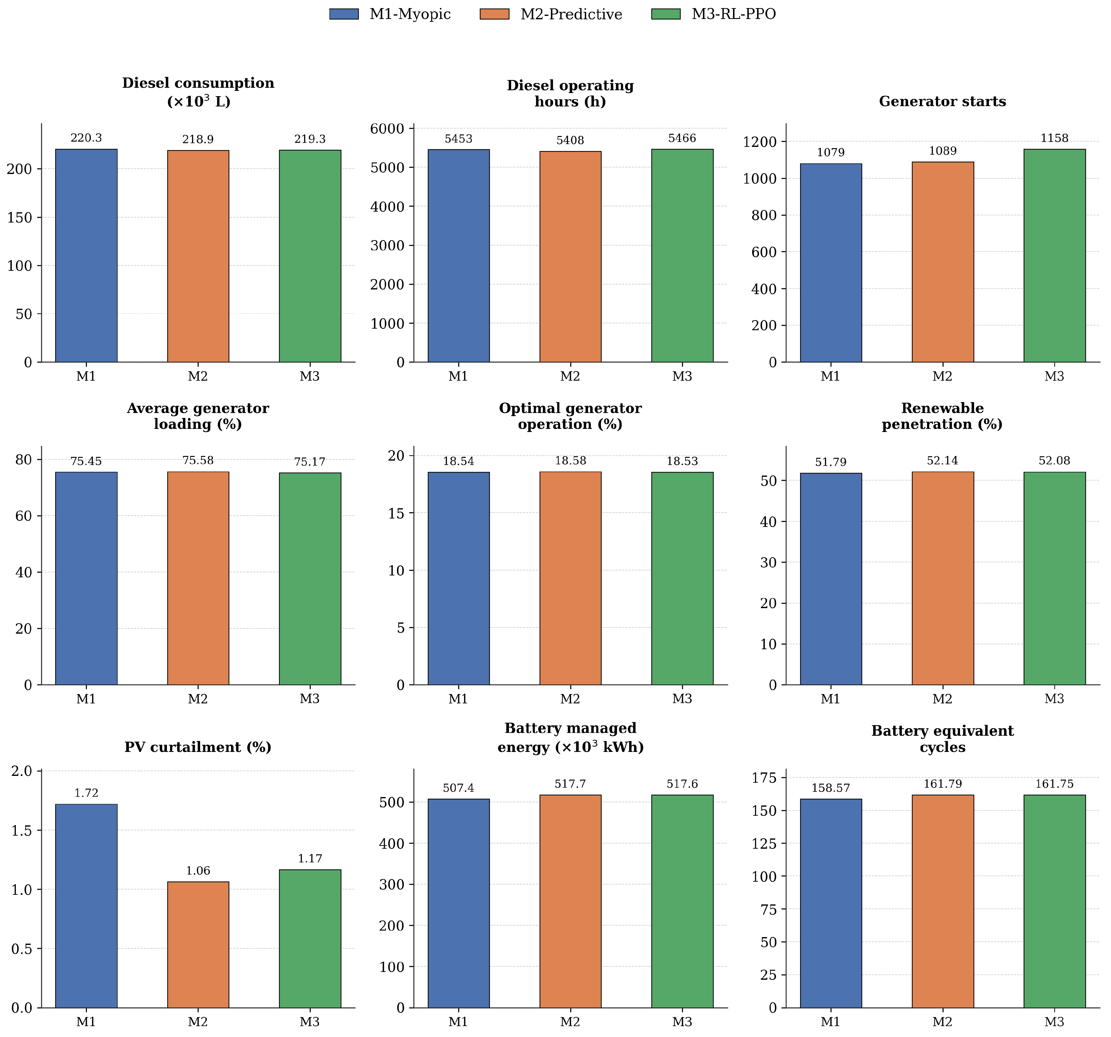To complement the tabulated results and improve visual interpretability, Figure 4 presents a condensed comparison of all nine performance indicators across the three EMS strategies, allowing a direct visual assessment of the relative differences among methods.

The annual results show that, unlike scenarios with more constrained renewable resources, the three EMS strategies converge toward relatively similar diesel consumption values, differing by less than 0.7% from one another (218,863 L for M2 up to 220,291 L for M1). This indicates that, under the evaluated operating conditions, the three EMS strategies achieve very similar overall fuel consumption, suggesting that their main differences lie not in the total amount of diesel energy required, but in how generation, battery operation, and renewable energy are coordinated.

Although a 0.7% relative difference may appear modest at first glance, its practical significance deserves a broader interpretation. In absolute terms, this 0.7% corresponds to approximately 1427 L of diesel saved per year by M2 relative to M1 in the evaluated Surpresa system, representing roughly R$9850/year at the diesel price adopted in this study (Section 3.3), a modest but non-negligible sum for a small-to-medium isolated microgrid, which accumulates over a multi-year operating horizon. More importantly, this saving is obtained at essentially zero marginal operating cost: once implemented, M2 and M3 require no additional effort, personnel, or real-time intervention relative to M1, since the decision itself is computed automatically and near-instantaneously at each simulation step, with the added complexity confined to the offline design and training stage rather than to day-to-day operation. Consequently, even a small percentage gain in fuel efficiency is obtained essentially for free from an operational standpoint, once the upfront modeling investment has been made. This percentage gain is also expected to scale with system size: for larger isolated microgrids with proportionally larger diesel consumption, the same 0.7% relative improvement would translate into substantially larger absolute savings, potentially reaching hundreds of thousands of Reais per year, making the practical value of adopting M2 or M3 considerably more significant at larger scales than the Surpresa case study alone suggests. This economic reading is consistent with, rather than in tension with, the more pronounced advantages observed for M2 and M3 in renewable-energy utilization and curtailment reduction discussed below.

Regarding generator operation, M2 presented the lowest diesel operating hours (5407.5 h) together with the highest average generator loading (75.58%), suggesting a more efficient dispatch that keeps the generators operating closer to their rated capacity for a shorter total duration. M3 exhibited the opposite trend, with the highest operating hours (5466.5 h), the lowest average loading (75.17%), and noticeably more generator starts (1158) than M1 (1079) and M2 (1089), yet its diesel consumption remained close to M2. This apparent inconsistency is consistent with an observed difference in how the PPO agent commits to battery decisions relative to M1 and M2: unlike the deterministic, forecast-anchored charge/discharge logic used by M1 and M2, the learned policy’s battery power trajectory displays visibly higher-frequency variation, as shown in the extreme-day analysis below, which is compatible with more frequent, shorter diesel-covered intervals rather than fewer, longer ones. We note, however, that this generator start-stop pattern is an emergent, indirect outcome of the interaction between the learned battery policy and the shared rule-based physical layer, rather than a directly controlled decision, and that attributing it to a single underlying cause, such as the reward formulation, training stochasticity, or the network architecture, from a single trained policy carries a genuine risk of causal confounding. We therefore present this explanation as an observationally motivated interpretation consistent with the data, rather than as an established causal mechanism; disentangling the actual cause would require targeted ablations (e.g., reward-shaping variants, comparison against a synthetic reactive non-RL battery policy with matched setpoint variance, or across-seed retraining), which we identify as a direction for future work. Because total diesel energy is governed primarily by the cumulative residual load rather than by how that load is segmented into generator runs, this more fragmented commitment pattern raises the start count without a corresponding fuel penalty, effectively trading generator wear for a dispatch style that emerged from reward feedback centered on instantaneous power balance rather than start-stop minimization. The optimal generator operation indicator remained fairly similar across all methods (18.53–18.58%), showing that none of the strategies substantially prioritized operation within the generators’ most efficient loading range.

The renewable energy and battery indicators reveal a more consistent advantage for M2 and M3 over M1. Both achieved higher renewable penetration (52.14% and 52.08%, respectively, versus 51.79% for M1) and lower photovoltaic curtailment (1.06% and 1.17%, versus 1.72% for M1), together with greater battery throughput (517,715.64 kWh and 517,610.96 kWh managed, versus 507,420.91 kWh for M1). These three indicators move together because they share the same underlying mechanism: without any anticipation of future PV availability or load behavior, M1 has no basis for deciding, in the moment PV surplus appears, whether to reserve battery headroom for it or let it curtail; forecasting (M2) and learned state-awareness (M3) both provide that anticipation, and consequently direct more surplus into the battery rather than curtailing it. The higher battery cycling this implies for M2 and M3 (161.79 and 161.75 equivalent cycles, versus 158.57 for M1) is therefore not an independent finding but the direct counterpart of their improved renewable utilization, and represents a trade-off against expected battery degradation that should be weighed alongside the fuel and curtailment gains.

Taken together, these results show that M2 and M3 are energetically comparable but operationally distinct: M2 reaches its performance through fewer, more deliberate generator cycles, while M3 reaches similar diesel consumption and renewable utilization through a more fragmented, reactive dispatch with substantially more generator starts. This distinction matters because annual aggregate indicators alone, such as diesel consumption or renewable penetration, would suggest M2 and M3 are nearly interchangeable, while the start-stop and loading behavior indicates they place different demands on equipment lifetime and maintenance. M1, in turn, is the most conservative of the three in both respects: lowest battery cycling and fewest generator starts, but also the lowest renewable utilization, since it lacks any mechanism to anticipate and capture PV surplus before it must be curtailed.

These findings indicate that EMS evaluation should not rely on a single performance indicator or exclusively on aggregate energy metrics: a comprehensive assessment must consider the interaction between fuel efficiency, renewable utilization, and equipment operating behavior. This distinction becomes particularly relevant when moving from simulation-based energy assessment toward practical microgrid deployment, where equipment lifetime, maintenance requirements, and battery degradation can be as important as fuel savings and renewable penetration.

3.2. Operational Analysis Under Extreme Days

In addition to the annual aggregated evaluation, detailed operational analyses were performed under extreme photovoltaic generation conditions to investigate the mechanisms underlying the differences observed among the EMS strategies. Two representative operating conditions were selected: the day with the highest photovoltaic generation and the day with the lowest photovoltaic generation during the evaluation year. These scenarios provide complementary perspectives on EMS operation. The high-PV condition represents a scenario with greater renewable availability and, consequently, greater flexibility for coordinating PV generation, battery storage, and diesel generation. In contrast, the low-PV condition represents a highly constrained operating environment in which the limited renewable resource restricts battery charging opportunities and increases the dependence on diesel generation.

The selected days were evaluated using complete power dispatch curves together with battery SOC and generator operation profiles. This analysis makes it possible to identify differences in battery charging and discharging behavior, generator scheduling, PV curtailment, and SOC management that may not be apparent from the annual aggregated indicators. More importantly, the comparison between the two extreme conditions allows the influence of renewable availability on the effectiveness and differentiation of the EMS strategies to be assessed.

3.2.1. Best PV Day

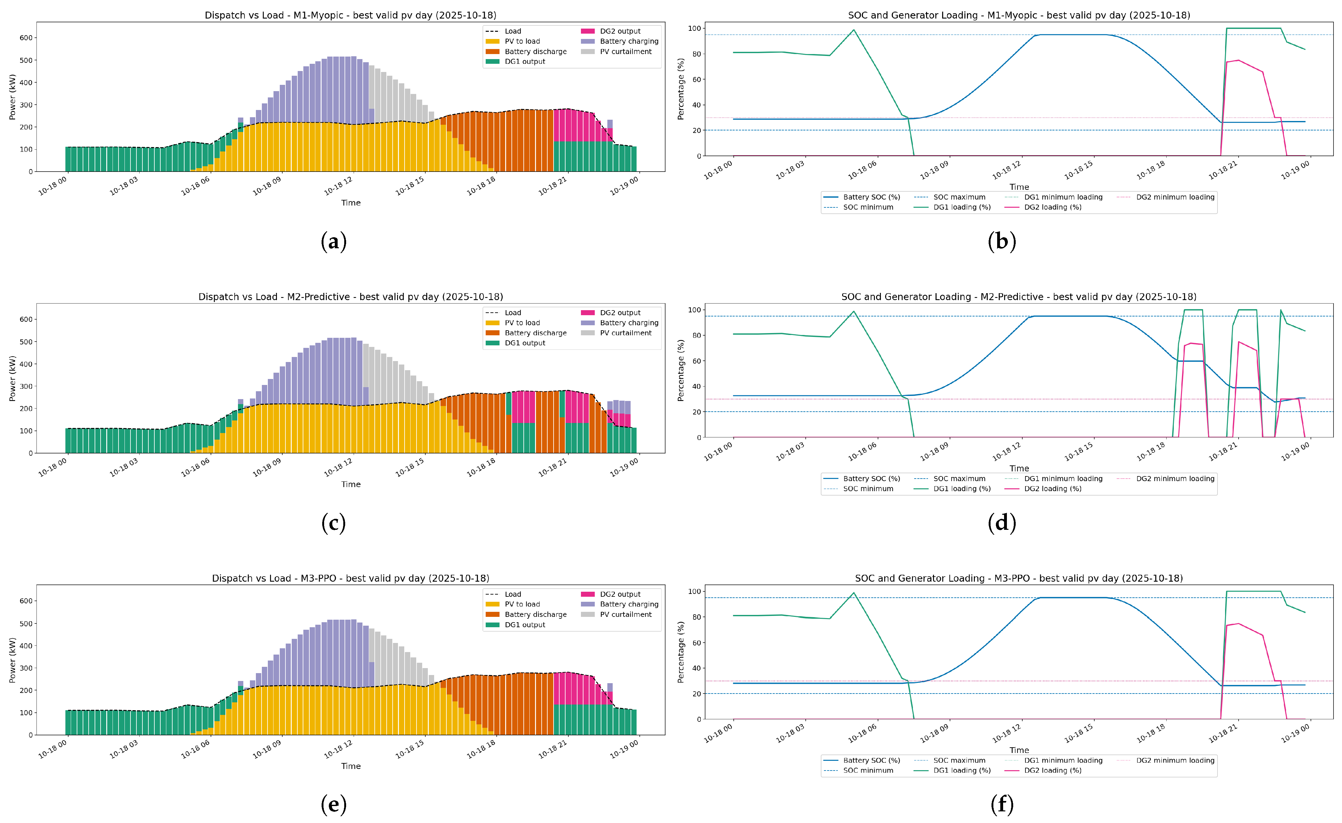
Figure 5 presents the operational behavior of the evaluated EMS strategies during the day with the highest photovoltaic generation (19 October 2025). For each method, the left panel shows the power balance among photovoltaic generation, load demand, battery operation, diesel generator dispatch, and curtailed energy, while the right panel presents the corresponding battery SOC trajectory together with the generator loading profile.

During the first half of the day, all three methods exhibit essentially identical operating patterns under this highly favorable renewable generation condition. Photovoltaic generation supplies a large portion of the demand during daylight hours, while the BESS absorbs the available surplus energy, reaching its upper SOC limit around midday, after which the excess photovoltaic generation that cannot be stored is curtailed. Up to this point, the dispatch and SOC curves of M1, M2, and M3 are visually indistinguishable.

The methods begin to diverge in the evening, once the battery starts discharging to support the load and photovoltaic generation is no longer available. Method M1 follows a predominantly reactive strategy, discharging the battery continuously and rapidly once the evening period begins. The SOC decreases steadily from its upper limit down to the lower operating threshold in a single, largely uninterrupted discharge, after which the diesel generators resume dispatch to supply the remaining load for the rest of the night.

Method M3 reproduces essentially the same evening behavior as M1, discharging the battery in a comparable manner and reaching the lower SOC limit at a similar point in the evening, with the diesel generators subsequently taking over the load.

Method M2 is the strategy that most clearly departs from this pattern. Instead of discharging the battery in a single continuous event, the Predictive strategy manages the evening discharge more conservatively, interleaving battery support with diesel generation and allowing the SOC to decrease more gradually, in a step-wise manner, rather than depleting the battery all at once. As a result, the diesel generators are engaged earlier and more frequently, cycling on and off in shorter intervals throughout the evening, while the battery is preserved at a comparatively higher SOC for a longer period. This more conservative use of the stored energy allows M2 to end the day with a higher battery SOC than M1 and M3, which is a favorable outcome, since it leaves the battery better positioned to support the load at the beginning of the following day, before photovoltaic generation becomes available again.

Overall, the results indicate that under conditions of abundant photovoltaic generation, all EMS strategies behave equivalently during the charging phase of the day, effectively utilizing the available renewable energy and storage resources. Furthermore, all methods respected the minimum diesel generator loading constraint, ensuring that the generators operated above 30% of their rated capacity whenever dispatched. The distinguishing behavior among the strategies emerges specifically during the evening discharge period, where M2’s more deliberate battery management trades a higher short-term reliance on diesel generation for improved battery availability at the end of the day.

Table 8. Quantitative comparison of generator operation and battery utilization for the highest photovoltaic generation day (18 October 2025).

Indicator	M1 (Myopic)	M2 (Predictive)	M3 (PPO-RL)
Diesel consumption (L)	376.54	393.41	376.54
Diesel operating hours (h)	13.5	14.25	13.5
DG1 starts	2	4	2
DG2 starts	1	3	1
Total generator starts	3	7	3
Battery charged energy (kWh)	1125.82	1103.86	1136.98
Battery discharged energy (kWh)	1045.31	1023.63	1045.31
PV curtailment (kWh)	435.16	500.32	424.00

quantifies these differences. M2 consumed slightly more diesel fuel (393.41 L versus 376.54 L for M1 and M3) and accumulated more diesel operating hours (14.25 h versus 13.5 h), consistent with the earlier and more frequent generator engagement described above. This difference is concentrated in the number of generator starts: M2 triggered 7 starts (4 for DG1, 3 for DG2) against only 3 for M1 and M3 (2 for DG1, 1 for DG2), directly reflecting the step-wise, interleaved discharge pattern adopted by the Predictive strategy instead of the single continuous discharge event observed for M1 and M3. Correspondingly, M2 discharged less battery energy over the day (1023.63 kWh versus 1045.31 kWh for M1 and M3), confirming that the battery was preserved at a comparatively higher state of charge, at the cost of the additional generator cycling and fuel consumption quantified above. PV curtailment also differed slightly among the strategies (500.32 kWh for M2 versus 424.0–435.16 kWh for M1 and M3), reflecting small differences in the timing of battery charging near the midday SOC ceiling.

3.2.2. Worst PV Day

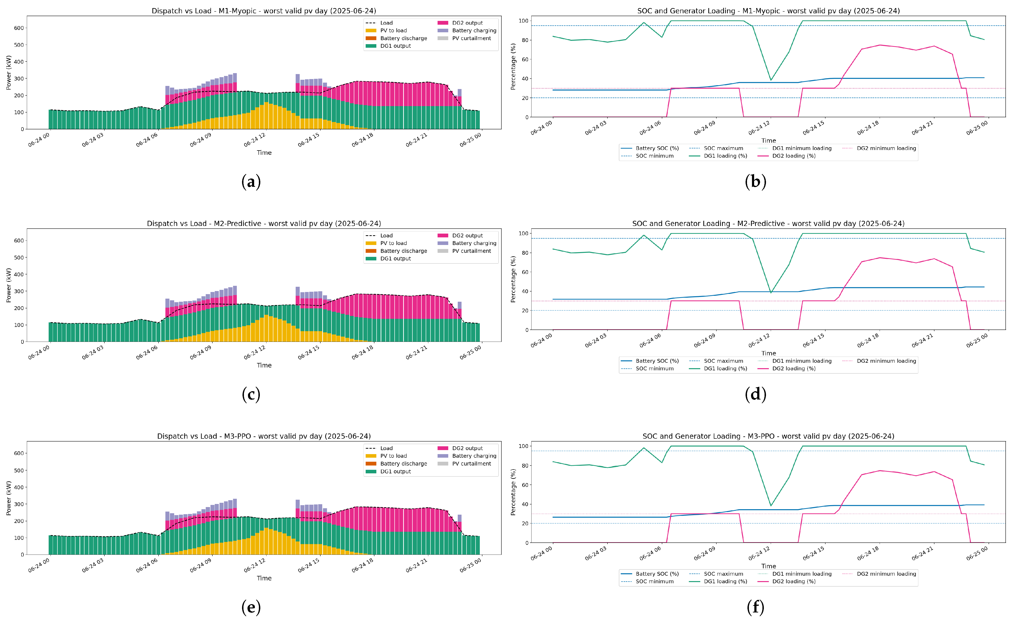
Figure 6 presents the operational behavior of the EMS strategies during the day with the lowest photovoltaic generation (24 June 2025). This scenario represents a particularly challenging operating condition, as the microgrid has very limited access to renewable generation and, consequently, very limited opportunities to recharge the battery from PV. Under these conditions, the flexibility available to the EMS is substantially reduced, forcing the system to rely predominantly on the diesel generators to maintain the power balance.

In contrast to the highest-PV day, where the availability of solar energy provides greater flexibility for coordinating PV generation, battery charging, and diesel operation, the low-PV condition leaves little room for such coordination. The battery receives only limited charging energy during the day, resulting in a gradual increase in SOC from approximately 28% to 41%. Consequently, battery operation becomes highly constrained, while the diesel generators assume the dominant role in supplying the load.

Method M1 operates DG1 for most of the day, generally at a relatively high loading level, while DG2 is activated during periods of increased demand in the early morning, around midday, and during the late afternoon and evening. The limited PV availability prevents substantial battery charging, and the battery therefore has little opportunity to contribute significantly to the dispatch.

Method M2 exhibits an operational trajectory very similar to that of M1, including comparable generator activation patterns and SOC evolution. Although M2 incorporates predictive information, the forecast-based strategy provides limited additional benefit in this scenario because the fundamental constraint is not a lack of anticipation, but the scarcity of available renewable energy. With insufficient PV generation to significantly alter the energy balance, the optimizer is naturally driven toward a generator-dominated solution.

Method M3 follows the same general behavior, with DG1 and DG2 assuming the primary role in load supply and the battery remaining constrained by the limited renewable charging opportunities. As a result, the differences among the three strategies become minimal, and their dispatch trajectories and SOC profiles closely overlap.

Table 9. Quantitative comparison of generator operation and battery utilization for the lowest photovoltaic generation day (24 June 2025).

Indicator	M1 (Myopic)	M2 (Predictive)	M3 (PPO-RL)
Diesel consumption (L)	1074.82	1074.82	1074.82
Diesel operating hours (h)	24.0	24.0	24.0
DG1 starts	1	1	1
DG2 starts	2	2	2
Total generator starts	3	3	3
Battery charged energy (kWh)	214.98	214.98	214.98
Battery discharged energy (kWh)	0.0	0.0	0.0
PV curtailment (kWh)	0.0	0.0	0.0

quantifies this convergence. Unlike the highest-PV day, where M2 diverged from M1 and M3 in diesel consumption, operating hours, and generator starts, all three strategies produce numerically identical results on the lowest-PV day: 1074.82 L of diesel consumption, 24 h of diesel operating hours, 1 start for DG1 and 2 starts for DG2, and identical battery charged energy (214.98 kWh), with no battery discharge recorded for any strategy. This exact numerical coincidence, rather than a mere qualitative resemblance, has a direct explanation in the architecture of the simulation framework: M1, M2, and M3 differ only in the higher-level decision layer that determines the battery power setpoint (myopic rule, forecast-based heuristic, or PPO policy, respectively), while diesel-generator commitment and dispatch are always resolved by the same common physical EMS layer, subject to the same operational constraints (minimum generator loading, ramping, and startup logic). Under the low-PV condition analyzed here, the battery has essentially no PV surplus available to charge from and is therefore left with no meaningful degrees of freedom to exploit, regardless of which decision layer is generating the battery setpoint; consequently, the three battery policies converge to the same near-zero-flexibility action, and the common physical EMS layer resolves the resulting diesel dispatch identically for all three strategies. In other words, once the decision problem collapses to the physical layer, differences in the upstream decision-making logic no longer have any input to act upon, which is precisely why the results are not merely similar but numerically identical.

This behavior highlights an important characteristic of the EMS strategies under adverse renewable conditions. When photovoltaic generation is severely restricted, the system loses much of the operational flexibility that would otherwise allow the different control strategies to exploit forecasting, optimization, or learning capabilities. In practical terms, all methods are subject to the same physical limitation: there is insufficient renewable energy to charge the battery and displace diesel generation. Therefore, the similarity among M1, M2, and M3 in this scenario should not be interpreted as a lack of effectiveness of the more advanced strategies, but rather as a consequence of the constrained operating environment.

Despite these limitations, all three methods successfully maintain the power balance and satisfy the minimum generator loading constraint throughout the day. The results demonstrate that, under extremely low-PV conditions, the EMS strategies converge toward a similar and reliable generator-led operating mode. This contrasts with the highest-PV scenario, in which the greater availability of renewable energy creates more opportunities for strategic differences in battery utilization and diesel dispatch. Thus, the comparison between the best- and worst-PV days demonstrates that the effectiveness of advanced EMS strategies is strongly dependent on the degree of operational flexibility provided by renewable generation. When PV availability is high, the EMS has greater freedom to coordinate storage and diesel generation, allowing differences between control strategies to emerge. Conversely, when PV availability is severely restricted, the lack of renewable energy constrains the feasible operating space and drives all strategies toward a similar generator-dominated solution.

This convergence has a direct practical implication for the deployment of advanced EMS strategies in isolated microgrids: the marginal value of forecasting (M2) or learning-based control (M3) over a simple myopic rule (M1) is not constant throughout the year, but is concentrated in periods of moderate-to-high renewable availability, and vanishes precisely when operational flexibility is most needed, during prolonged low-irradiance conditions. In other words, the additional modeling complexity, computational cost, and engineering effort associated with predictive or RL-based EMS are not justified by their performance under fuel-constrained, low-PV operation, since no control strategy can extract flexibility that the physical system does not provide. From a system-planning perspective, this suggests that the primary lever for improving performance during low-PV periods is not a more sophisticated EMS, but rather structural measures such as increased PV and battery capacity, hybridization with complementary renewable sources, or demand-side management, whereas the choice among M1, M2, and M3 is expected to matter mainly for maximizing renewable utilization and reducing generator cycling during the remainder of the year. This does not diminish the practical value of advanced EMS strategies, since real operation spans the full range of renewable availability rather than only its worst-case extreme, but it does clarify that their benefit should be evaluated, and communicated to practitioners, as a seasonally conditional rather than uniformly year-round advantage.

3.3. Economic Analysis of the Surpresa Hybridization

In addition to the operational and energetic evaluation of the EMS strategies, a simplified economic analysis was performed to assess the financial attractiveness of hybridizing the diesel-based system of Surpresa with photovoltaic generation and battery energy storage. All monetary values presented in this subsection are expressed in Brazilian Reais (R$, BRL), consistent with the currency adopted in the HOMER Pro techno-economic assessment. Since the diesel generator fleet is an existing asset of the locality, this analysis focuses exclusively on the incremental investment required to add the PV and BESS components to the current diesel-only system, rather than on the cost of the complete microgrid.

As the M2 (Predictive) strategy achieved the lowest annual diesel consumption among the three EMS strategies evaluated in this study, it was adopted as the reference operating condition for the hybridized scenario. To quantify the diesel savings enabled by hybridization, a diesel-only baseline was additionally simulated using the same EMS decision logic and operational constraints, but with the PV and BESS components removed from the physical model, so that the electrical load is supplied exclusively by the diesel generator fleet. Under this diesel-only configuration, the annual fuel consumption for 2025 was 457,635.87 L, compared with 218,863.19 L obtained by M2 in the hybridized configuration (Table 6). Assuming a diesel price of R$6.90/L, this corresponds to an annual fuel cost of approximately R$3,157,687.50 for the diesel-only case and R$1,510,156.01 for the hybridized case, yielding an annual diesel cost saving of approximately R$1,647,531.49 attributable to the PV-BESS hybridization.

The incremental investment associated with the hybridization was obtained from a HOMER Pro techno-economic simulation report of the Surpresa hybridization project, considering only the PV, BESS, and power converter components. The capital cost of these components totals approximately R$4.62M (R$2.33M for the BESS, R$2.22M for the PV system, and R$67,724 for the converter), while their combined annual operation and maintenance (O&M) cost, obtained from the annualized HOMER cost breakdown, totals approximately R$205,588/year.

Table 10. Economic inputs and resulting indicators for the hybridization analysis (HOMER Pro techno-economic assessment and EMS simulations).

Parameter	Value
PV capital cost	R$2.22M
BESS capital cost	R$2.33M
Converter capital cost	R$67,724
Total incremental CAPEX (PV + BESS + converter)	R$4.62M
Combined annual O&M (PV + BESS + converter)	R$205,588/year
Diesel price	R$6.90/L
Diesel-only annual consumption (no PV/BESS)	457,635.87 L
Hybridized annual consumption (M2)	218,863.19 L
Discount rate (Brazilian benchmark interest rate)	14% p.a.
Evaluation horizon	15 years
Internal Rate of Return (IRR)	30.7% p.a.
15-year NPV (at 14% p.a.)	R$4.24M
Simple payback period	3.2 years
Discounted payback period (at 14% p.a.)	4.6 years

All monetary values are expressed in Brazilian Reais (R$, BRL).

summarizes the economic inputs adopted in this analysis, all of which are sourced from this HOMER Pro report except for the diesel-only and hybridized annual consumption values, which were obtained from the EMS simulations conducted in this study (Section 3); the same table also reports the resulting economic indicators (IRR, NPV, and payback periods) obtained from the cash flow analysis described below.

A simplified discounted cash flow analysis was then conducted over a 15-year horizon, taking the incremental CAPEX as the initial outflow (year 0) and the net annual cash flow, the annual diesel cost savings net of the PV-BESS O&M cost (R$1,647,531.49 minus R$205,588 = R$1,441,943.49/year), as a constant annual inflow from year 1 to year 15. Diesel price, O&M costs, and load demand were assumed constant in real terms over the evaluation horizon, and no replacement costs were considered within the 15-year window, consistent with the negligible replacement costs reported by HOMER for these components. The Internal Rate of Return (IRR) was computed as the discount rate that sets the net present value (NPV) of this cash flow series to zero, and the resulting IRR was compared with the adopted discount rate of 14% p.a., representative of the benchmark interest rate in Brazil, to assess whether the hybridization investment is economically attractive relative to the opportunity cost of capital. In addition to the simple payback period (CAPEX divided by the constant net annual cash flow), a discounted payback period was computed as the year in which the cumulative discounted cash flow, using the 14% discount rate, first becomes non-negative, providing a stricter payback estimate that accounts for the time value of money.

The analysis indicates an IRR of approximately 30.7% p.a. for the incremental PV-BESS investment, substantially higher than the 14% p.a. discount rate, a simple payback period of approximately 3.2 years, and a discounted payback period (at the 14% discount rate) of approximately 4.6 years. At the 14% discount rate, the 15-year NPV of the hybridization is approximately R$4.24M, positive and consistent with the IRR and payback results.

These results indicate that, despite the three EMS strategies achieving comparable annual diesel consumption (Section 3), the hybridization of the Surpresa microgrid is economically attractive under the evaluated assumptions, since the avoided diesel expenditure alone is sufficient to recover the incremental PV-BESS investment well within the 15-year horizon and to substantially exceed the return offered by the reference discount rate.

To assess the robustness of this conclusion, a sensitivity analysis was performed by independently varying the diesel price and the combined PV-BESS O&M cost by ±10% and ±20% around their base values, while keeping all other inputs (CAPEX, consumption values, and evaluation horizon) unchanged; the resulting IRR and simple payback period for each scenario are summarized in

Table 11. Sensitivity of the IRR and simple payback period to variations in diesel price and PV-BESS O&M cost (base case: diesel price = R$6.90/L, O&M = R$205,588/year).

Scenario	IRR (% p.a.)	Simple Payback (Years)
Diesel price − 20%	23.0	4.15
Diesel price − 10%	26.9	3.62
Base case	30.7	3.20
Diesel price + 10%	34.4	2.87
Diesel price + 20%	38.1	2.61
O&M cost − 20%	31.6	3.11
O&M cost − 10%	31.1	3.16
Base case	30.7	3.20
O&M cost + 10%	30.2	3.25
O&M cost + 20%	29.7	3.30
Combined pessimistic (diesel − 20%, O&M + 20%)	22.0	4.31
Combined optimistic (diesel + 20%, O&M − 20%)	39.0	2.55

. It is worth noting that the discount rate does not directly enter the IRR calculation, since the IRR is, by definition, the discount rate at which the NPV of the cash flow series equals zero and is therefore determined solely by the magnitude and timing of the cash flows themselves; the discount rate instead affects the economic attractiveness margin, i.e., how the computed IRR compares against the adopted opportunity cost of capital, and the resulting NPV. Accordingly, the sensitivity of the NPV to the discount rate was assessed separately by recomputing the 15-year NPV of the base-case cash flow series (i.e., without varying diesel price or O&M cost) across a range of discount rates from 8% to 30% p.a.

The results in Table 11 show that the IRR is substantially more sensitive to variations in the diesel price than to variations in the O&M cost. A ±20% variation in diesel price shifts the IRR from 23.0% to 38.1% p.a. (a range of approximately 15 percentage points), since diesel price directly scales the annual diesel cost savings that constitute the entire economic benefit of the hybridization in this analysis. In contrast, the same ±20% variation in the O&M cost shifts the IRR only from 29.7% to 31.6% p.a. (a range of about 2 percentage points), because the O&M cost is a comparatively small deduction from the annual diesel savings rather than the primary driver of the net cash flow. Even under the combined pessimistic scenario (20% lower diesel price together with 20% higher O&M cost), the IRR remains at approximately 22.0% p.a., still well above the 14% discount rate, and the simple payback period remains below 4.5 years. Regarding the discount rate, since it does not alter the underlying cash flows, it leaves the IRR itself unchanged at 30.7% p.a.; however, it directly affects the computed NPV, which decreases from approximately R$7.72M at a 8% discount rate to approximately R$0.09M at a 30% discount rate, the latter being close to the breakeven point at which the discount rate approaches the IRR itself. Overall, the NPV of the hybridization remains positive for all discount rates below the IRR (30.7%), indicating that the investment is expected to remain economically attractive across a wide range of plausible discount-rate assumptions, and that the conclusion of economic feasibility is most sensitive to the assumed diesel price, followed by the O&M cost, and is inherently robust to the choice of discount rate within realistic ranges for the Brazilian context.

The main assumptions and limitations of this economic analysis should be made explicit. First, the analysis assumes constant diesel prices, O&M costs, and electrical load over the 15-year evaluation horizon, in real terms; potential diesel price escalation or reduction, inflationary effects on O&M costs, and future load growth are not considered, and could respectively improve or worsen the computed IRR and payback period, as quantified above. Second, no battery replacement cost is included within the 15-year evaluation horizon. This is not an oversight but a deliberate modeling choice: battery technologies typically adopted in isolated microgrid applications of this scale (e.g., LiFePO₄) are commonly rated for expected service lives exceeding 15 years under the cycling conditions observed in this study (approximately 160 equivalent cycles/year, well within the manufacturer-rated cycle life at the depth-of-discharge levels enforced by the EMS constraints), consistent with the replacement schedule reported by HOMER Pro for the evaluated system size, in which the BESS capital cost is amortized once over the full evaluation horizon with no additional replacement events. Under this assumption, the annual BESS operation and maintenance (O&M) cost already included in the cash flow is sufficient to capture the ongoing cost of maintaining the storage system over the horizon considered, without requiring an explicit degradation model or a mid-horizon replacement outflow. We note, nonetheless, that a shorter effective battery lifetime than assumed, e.g., due to site-specific thermal conditions or duty cycles more severe than anticipated, would reduce the computed economic attractiveness, and that extending the analysis beyond 15 years would eventually require accounting for battery replacement. Third, the economic benefit is attributed exclusively to avoided diesel fuel expenditure and does not include potential additional value streams, such as reduced maintenance costs associated with lower diesel operating hours, avoided greenhouse gas emissions, or improved reliability; the analysis is therefore conservative in this respect. Fourth, financing costs, taxes, and import duties on PV and BESS equipment are not explicitly modeled, and the capital and O&M costs are taken directly from the HOMER Pro techno-economic assessment, which reflects the cost assumptions and equipment pricing adopted therein and may not fully capture local market variability. Finally, the diesel savings used in this analysis correspond specifically to the M2 (Predictive) strategy, which achieved the lowest annual diesel consumption among the three EMS strategies evaluated; since the differences in diesel consumption among M1, M2, and M3 are small (less than 0.7%, Section 3), the economic conclusions are not expected to be sensitive to which of the three EMS strategies is ultimately adopted, but they are specific to the operating conditions, irradiance and load profiles, and equipment costs considered in this study, and should not be directly extrapolated to other isolated microgrid sites without re-evaluation. For these reasons, the presented analysis should be interpreted as a first-order indication of economic feasibility rather than a complete financial assessment.

4. Conclusions

This study investigated three EMS strategies for an isolated hybrid microgrid composed of photovoltaic generation, battery energy storage, and diesel generation representative of the District of Surpresa in the Brazilian Amazon. A Myopic strategy (M1), a Predictive strategy (M2), and a PPO-RL strategy (M3) were implemented within a common physical simulation framework and evaluated over a complete year at 15 min resolution. The use of identical component models and operational constraints ensured that the observed differences were primarily associated with the EMS decision-making strategies.

The annual results showed that the three methods achieved very similar diesel consumption, with a difference of less than 0.7% between the best and worst cases. M2 achieved the lowest fuel consumption (218,863.19 L), the lowest diesel operating time (5407.5 h), and the highest average generator loading (75.58%). More pronounced differences were observed in renewable-energy utilization. M2 achieved the highest renewable penetration (52.14%) and the lowest PV curtailment (1.06%), followed closely by M3, while M1 exhibited the most conservative battery utilization and the highest curtailment.

An important finding is that similar aggregate energy performance does not necessarily imply similar operational performance. M2 and M3 achieved nearly equivalent results in terms of diesel consumption, renewable penetration, PV curtailment, and battery utilization, but their operational behaviors differed substantially. M2 combined lower generator operating hours with higher battery cycling, whereas M3 exhibited a considerably higher number of generator starts. These results demonstrate that EMS evaluation should not rely exclusively on fuel consumption or renewable penetration, but should also consider battery cycling, generator loading, and start-stop behavior, since these factors have direct implications for equipment degradation and maintenance.

The extreme-day analysis, presented as a qualitative, illustrative case study, further helped clarify the operational mechanisms behind the annual, full-year quantitative results discussed above. During the highest-PV day, abundant solar generation provided sufficient flexibility for differences among the strategies to emerge, particularly during the evening battery discharge period. M2 adopted a more conservative battery-discharge strategy, preserving a higher SOC by coordinating battery support with earlier diesel operation. Conversely, during the lowest-PV day, the lack of available photovoltaic energy severely restricted battery charging opportunities and forced all methods toward a similar diesel-dominated operating mode. Thus, advanced EMS strategies have greater opportunity to differentiate their operation when sufficient renewable energy and storage flexibility are available, a mechanism consistent with, and illustrative of, the annual aggregate pattern rather than a finding established by these two days alone.

Overall, M2 provided the best aggregate balance among fuel consumption, renewable utilization, PV curtailment, and generator operation, while M3 achieved comparable energy performance through a distinct operational policy. M1, despite its simpler and more conservative operation, was less effective at exploiting available photovoltaic energy. The results therefore indicate that the main advantage of advanced EMS strategies in the evaluated microgrid lies not necessarily in large reductions in annual diesel consumption, but in improving the coordination and utilization of available energy resources. As a direction for future work, the EMS strategies evaluated in this study could be extended to support distributed energy trading among isolated microgrid users, an area in which privacy-preserving and blockchain-based matching mechanisms have recently shown promise for enabling secure and decentralized peer-to-peer transactions in smart grids [35], which could be particularly relevant in isolated or remote microgrid contexts where trust and transparency among participants are critical.

The analysis is based on a single microgrid configuration, location, and evaluation year: the Surpresa system, with its specific PV, BESS, and diesel generator sizing, real 2025 irradiance and load profiles, and the operational constraints described in Section 2. The reported magnitudes, namely the 0.7% diesel-consumption spread among strategies, the renewable-penetration and curtailment values, and the specific generator start-stop counts, are therefore particular to this system and should not be directly transferred to other isolated microgrids without re-evaluation under their own resource, load, and equipment conditions. We expect the qualitative mechanisms identified here to generalize conceptually to other diesel-PV-battery microgrids of a comparable scale, namely that forecasting and learning-based anticipation provide operational benefits that scale with the renewable flexibility available in the system, and that these benefits are concentrated in periods of moderate-to-high PV availability, but confirming this would require evaluating additional sites with different renewable resources, load profiles, and component sizing, which we identify as a natural extension of this work.

Two further directions are left for future work. First, the Random Forest forecasting module adopted by M2 could be replaced or complemented by LSTM-RNN architectures, which may better capture temporal dependencies and short-term cloud-induced transients in GHI, as well as temporal variations in demand. This could improve the accuracy of the short-term forecasts used by the predictive EMS and consequently reduce the impact of forecast errors on energy dispatch decisions. Moreover, combining LSTM-based forecasting with robust design methodologies such as DFSS could improve the robustness of the EMS against forecasting uncertainties and unexpected operating conditions, as demonstrated in DFSS/LSTM-based energy management strategies for hybrid electric vehicles [36]. Second, the EMS framework could be extended with resilience- and security-aware mechanisms based on digital-twin-based resilient consensus control approaches [37,38]. Such mechanisms could enhance the framework’s ability to detect, tolerate, and mitigate the effects of communication failures or cyber-threats in networked microgrids, which becomes increasingly relevant as isolated microgrids rely on networked communication and remote monitoring infrastructure.

Beyond the operational comparison among EMS strategies, a simplified economic analysis of the Surpresa hybridization itself indicated that the incremental investment in PV and battery storage is economically attractive when evaluated against the existing diesel-only configuration. Using the diesel savings achieved by M2 as the reference economic benefit, the estimated internal rate of return of approximately 30.7% p.a. considerably exceeds the 14% p.a. benchmark interest rate, with a simple payback period of approximately 3.2 years. This result reinforces that, independently of which EMS strategy is ultimately adopted, the hybridization of the Surpresa microgrid with photovoltaic generation and battery storage is a sound investment on its own, while the choice among M1, M2, and M3 remains primarily an operational rather than an economic decision within the range of strategies evaluated.