Domain-Informed Structured Detection of As-Drilled Trajectory Transitions for Post-Well Conformance Assessment

Abstract

Post-well conformance assessment requires identifying the realized locations where an as-drilled trajectory changes between its principal inclination regimes; planned breakpoints are targets, not observations. We formulate this task as sparse event localization using domain-informed multiscale inclination features, planned-trajectory deviations, event-specific LightGBM models, a well-level Drop-presence model, and exact Build–Hold or Build–Hold–Drop decoding. The operational scope is restricted to completed, conventional single-cycle trajectories containing exactly one Build, exactly one Hold, and at most one Drop; build-only, repeated-transition, seven-section, and online trajectories are excluded. We evaluated 63 field wells, including 25 with Drop, by fixed five-fold well-level cross-validation. At the prespecified 60 m tolerance, the detector achieved a macro-F1 of 0.806 (95% confidence interval, 0.737–0.869), versus 0.616 for a derivative rule, 0.567 for change-point dynamic programming, and 0.615 for segmented regression. Its paired advantage over the strongest classical comparator was 0.190 (0.111–0.268). Build, Hold, and Drop F1 values were 0.984, 0.857, and 0.577. Drop-presence ranking was strong (average precision, 0.944), but only 15 of 22 emitted true Drops were localized within 60 m. All seven localization failures were late and spanned 115.9–347.5 m; they were associated with lower ranks of the labeled station score and weaker early inclination decline. On 47 matched wells, planned anchors achieved 0.281, versus 0.809 for the detector; sensitivity analysis over 324 anchor-rule configurations did not close this gap. Exact decoding guaranteed valid event order but produced the same predictions as greedy selection; thus, its demonstrated contribution on this dataset is output validity rather than localization-accuracy improvement. Validation was limited to 63 wells from a single competition-supplied field dataset; external multi-field generalization remains untested.

1. Introduction

Directional-well construction connects a geometric plan to a trajectory realized under formation, bottom-hole assembly (BHA), survey, and operational effects. Directional and horizontal drilling technologies have therefore developed alongside survey, steering, and automated planning systems that seek to place the wellbore within engineering and geological constraints [1,2,3,4,5]. Recent work spans observer-based and uncertainty-robust trajectory control [6,7], model-predictive deviation correction [8], and model-free toolface control [9]. Measurement-while-drilling surveys also carry instrument, magnetic, depth, and propagation uncertainties that are formalized in wellbore-positioning models and standards [10,11,12]. These studies establish an increasingly automated control stack, but primarily address how a future path should be generated or steered.

Data-driven methods have expanded this prospective view. Recurrent networks have been trained while drilling to predict inclination [13], random forests have been used to predict borehole trajectories [14], and downhole machine-learning estimates have supported drilling-position control [15]. A recent bit-projection system combined motor-yield prediction with directional-drilling advisories [16]. At the planning level, machine learning, reinforcement learning, and constrained multi-objective optimization have been used to generate or refine trajectories [3,17,18]; robust virtual-drilling studies additionally show how geological uncertainty can alter preferred well placement [19]. Post-well quality assessment asks a complementary retrospective question: where did the completed trajectory actually enter and leave its principal inclination regimes?

The distinction between planned and realized transitions matters because a design breakpoint is a target, not an observation of the completed trajectory. Using a planned Build, Hold, or Drop location as the corresponding as-drilled event can conceal delayed or early trajectory response and can propagate inconsistent transition records into multi-well databases. Recent work on automatic directional-drilling calibration likewise emphasizes that systematic steering behavior must be inferred from realized responses rather than assumed from the nominal command alone [20]. A reproducible post-well workflow should therefore preserve both locations and report their offset.

Data-driven drilling studies have demonstrated the value of machine learning for rate-of-penetration prediction and optimization [21,22] and for detecting drilling dysfunctions from depth-indexed measurements [23]. Multivariate time-series models have also been developed specifically for anomaly detection in drilling data [24]. Sparse transition localization is nevertheless different from continuous regression, anomaly scoring, or dense station classification. A completed well contains thousands of background stations but only two or three target events. The events must follow a restricted order, their physical separation is measured in depth rather than row number, and a Drop event is absent in many wells. Generic point-wise accuracy is consequently dominated by background and does not answer whether the transitions were localized.

Change-point, anomaly-detection, and depth-sequence methods provide relevant tools. Offline change-point analysis offers a broad family of cost, search, and penalty formulations for segmenting ordered signals [25], whereas modern anomaly-detection reviews distinguish point, contextual, and collective anomalies and emphasize the dependence of performance on representation and evaluation protocol [26,27]. In subsurface applications, multivariate change detection has been combined with machine learning to segment nonstationary well logs [28]; deep-kernel and spatiotemporal networks likewise exploit neighboring depth samples for lithofacies interpretation [29,30]. Statistical change-point methods can identify trend or distribution changes in engineering monitoring records [31], while dynamic time warping has been applied to depth-indexed log similarity [32]. For the present task, however, a useful output must associate event evidence with an explicit engineering sequence, distinguish an absent Drop from a poorly localized Drop, and retain planned-to-actual offsets. This motivates an event-specific formulation rather than background-dominated four-class station accuracy.

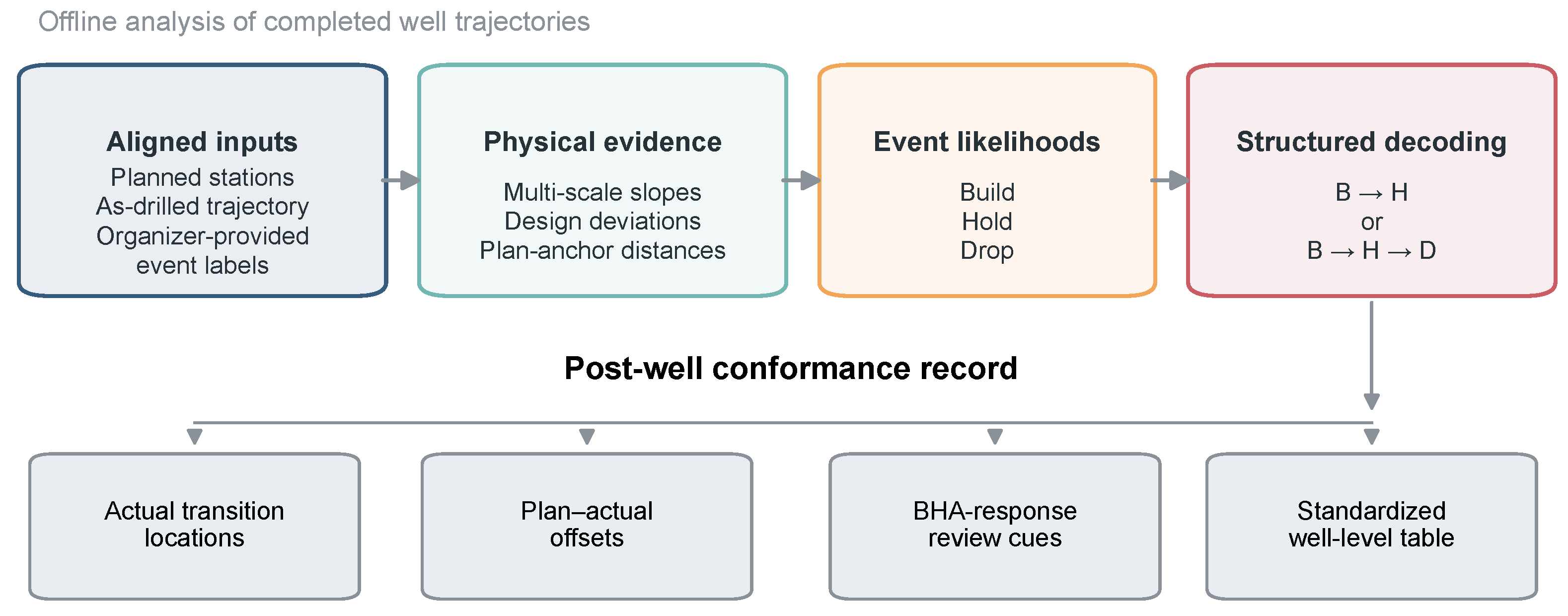
Here we present a domain-informed structured detector for offline analysis of completed well trajectories (Figure 1). It aligns sparse planned stations with as-drilled surveys and estimates event-specific likelihoods from physically motivated multiscale inclination descriptors. It then decodes either a Build–Hold or Build–Hold–Drop sequence. The method targets completed conventional trajectories containing exactly one Build, exactly one Hold, and at most one Drop. It excludes build-only records, repeated Build/Hold/Drop cycles, seven-section trajectories, and incomplete streaming trajectories. The experiments test localization accuracy, independent classical comparators, individual and grouped feature contributions, structured decoding, plan-anchor sensitivity, survey-station resolution, and measurement perturbation. They also separate Drop-presence errors from conditional localization errors and characterize the seven Drop failures.

2. Materials and Methods

2.1. Field Trajectory Records

The data were supplied to participants by the organizer of Sinopec’s First Artificial Intelligence Innovation Competition, Track 2, “Identification of Build, Hold, and Drop Conditions from Drilling-Trajectory Data” (competition identifier SINOPEC-02), through the official competition portal (historical URL: https://aicup.sinopec.com/; currently unavailable). The training file contained planned and as-drilled trajectory records together with organizer-provided key-point labels. The authors used the competition file unchanged for this study and did not publicly redistribute the source records.

The supplied field export contained 8603 rows from 64 wells. Rows without an as-drilled inclination measurement also lacked an event label; these 858 rows were not treated as trajectory observations, leaving 7745 labeled as-drilled stations. They were retained separately when they carried planned-trajectory values, because design and as-drilled stations were stored on different rows. The original depth-like field coordinate, XJS, was measured in metres and used for sorting, interpolation, and localization error. The median within-well XJS station spacing was $28.7$ m.

The organizer encoded background, Build, Hold, and Drop stations in the key-point field. Each event label occurred at one station, and the authors did not relabel, move, or adjudicate these stations. Build denotes the onset of the principal inclination increase, Hold the transition from build to approximately steady inclination, and Drop the onset of the principal inclination decrease. The competition materials available to the authors did not identify the annotators, their number or expertise, or an adjudication protocol. Inter-rater agreement could therefore not be assessed, and the supplied labels were treated as a single reference annotation set.

Operational inclusion required a completed as-drilled record with exactly one Build label, exactly one later Hold label, and zero or one still-later Drop label. Records missing Hold, containing repeated Build/Hold/Drop cycles, representing seven-section or other multi-cycle designs, or requiring online detection before well completion were outside the primary scope. All 64 wells contained a Build label, 63 contained a Hold label, and 25 contained a Drop label. The single build-only well was therefore excluded before fold construction and reserved as a scope-sensitivity case. This left 63 independent wells: 38 with Build–Hold and 25 with Build–Hold–Drop (

Table 1. Dataset and primary-analysis cohort. Event counts are also well counts because each included event type occurs once per well.

Quantity	Value
Source rows	8603
Labeled as-drilled stations	7745
All wells	64
Primary-scope wells	63
Build events	64
Hold events	63
Drop events	25
Primary Build–Hold wells	38
Primary Build–Hold–Drop wells	25
Wells with planned inclination stations	52
Median XJS station spacing	$28.7$ m

). Planned inclination stations were present in 52 of the 64 wells.

2.2. Event-Localization Task

For well w, let ${\mathbf{x}}_w=(x_1,\dots ,x_{n_w})$ denote ordered XJS stations and let ${\mathbf{z}}_w$ denote the corresponding as-drilled measurements. The target is the partial event map

$$T_w=\{B:x_B,H:x_H\}\mathrm{or}{T}_w=\{B:x_B,H:x_H,D:x_D\},$$

(1)

subject to $x_B<x_H<x_D$ when Drop is present. Build denotes the onset of the principal inclination increase, Hold the transition from build to approximately steady inclination, and Drop the onset of the principal inclination decrease. Planned anchors $P_w$ are stored separately from $T_w$ and are not used as ground-truth events.

2.3. Planned-to-As-Drilled Alignment

Planned inclination values were first extracted from all source rows, including rows without as-drilled measurements. For wells with at least two planned stations, the planned inclination was linearly interpolated to the as-drilled XJS grid inside the design support. Planned transition anchors were then obtained from the smoothed planned inclination gradient. Two consecutive stations with a gradient above ${0.05}^{\circ }$ per 30 m marked a candidate Build; after a minimum 60 m separation, two stations with an absolute gradient below ${0.045}^{\circ }$ per 30 m marked Hold; after a further 120 m, two stations below $-{0.05}^{\circ }$ per 30 m marked Drop. These transparent rules generated auxiliary anchors, not labels. They produced Build, Hold, and Drop anchors in 47, 46, and 20 primary wells, respectively.

2.4. Domain-Informed Station Features

Inclination was smoothed with an 11-station, second-order Savitzky–Golay filter [33]. The station representation contained 41 domain-informed variables in four cumulative groups. These variables encode trajectory geometry and engineering context but do not impose governing-equation residuals or hard physical constraints:

• G1, geometry (7 variables): inclination, normalized XJS position, sine and cosine of azimuth, a normalized auxiliary depth channel, inclination gradient, and gradient curvature;
• G2, multiscale context (17 additional variables): backward and forward linear slopes over 60 m, 120 m, and 240 m, their differences, centred slope variability and inclination ranges, and position relative to peak inclination;
• G3, design deviation (5 additional variables): design support, interpolated planned inclination and gradient, and signed and absolute inclination deviations;
• G4, planned anchors (12 additional variables): availability, signed and absolute XJS distance, and a 150 m Gaussian proximity kernel for each event type.

The workflow is explicitly offline: forward-window and full-well features are permitted because the complete trajectory is available. They would constitute future information in an online deployment.

2.5. Event Probability and Drop Presence Models

Separate LightGBM binary classifiers [34] estimated event probabilities. For event e and station i, the output was

$$p_e\left(i\right)=P(e\mathrm{at}\mathrm{station}i\mid {\mathbf{z}}_w),e\in \{B,H,D\}.$$

(2)

All model, preprocessing, and decoding hyperparameters are consolidated in

Table 2. Consolidated preprocessing, model, and decoder hyperparameters used in every outer fold.

Component	Fixed Setting
Inclination smoothing	Savitzky–Golay window 11 stations; polynomial order 2
Multiscale windows	60, 120, and 240 m backward and forward windows
Event LightGBM	Binary objective; 240 trees; learning rate 0.035; 15 leaves; maximum depth 5; minimum child samples 12
LightGBM regularization	Row subsampling 0.85; column subsampling 0.85; $L_1=0.15$; $L_2=0.8$
Station weighting	Training-fold negative-to-positive ratio, capped at 100
Drop-presence model	Standardized inputs; class-balanced logistic regression; $C=0.8$; maximum 2000 iterations
Drop decision	Probability threshold 0.5
Structured decoder	Minimum Build–Hold separation 60 m; minimum Hold–Drop separation 120 m
Reproducibility	Five fixed well-level folds; random seed 20260821

. Positive station weights were calculated only from the corresponding training fold, and all preprocessing and model fitting were repeated within each outer fold.

Because Drop was absent from 38 primary wells, event localization was separated from event presence. A class-balanced logistic model estimated a well-level Drop probability from the peak-to-tail inclination loss, post-peak negative-gradient summaries, the peak position, and planned Drop availability. A threshold of 0.5 selected the Build–Hold–Drop pattern; otherwise the decoder used Build–Hold.

2.6. Exact Structured Decoding

Class probabilities were clipped to $[{10}^{-6},1-{10}^{-6}]$, transformed to logits, and standardized within each well to give scores $s_B\left(i\right)$, $s_H\left(i\right)$, and $s_D\left(i\right)$. For a Build–Hold well, the decoder solved

$$({\widehat{i}}_B,{\widehat{i}}_H)=\arg \underset{i,j:x_j-x_i\ge 60}{\max }\left[s_B\left(i\right)+s_H\left(j\right)\right].$$

(3)

For a Build–Hold–Drop well, it solved

$$({\widehat{i}}_B,{\widehat{i}}_H,{\widehat{i}}_D)=\arg \underset{\begin{array}{c}i,j,k:\\ x_j-x_i\ge 60\\ x_k-x_j\ge 120\end{array}}{\max }\left[s_B\left(i\right)+s_H\left(j\right)+s_D\left(k\right)\right].$$

(4)

Distances are in metres of XJS. The implementation stores the best predecessor for each Hold and Drop state and backtracks from the terminal optimum. It is therefore a genuine dynamic program rather than top-K candidate enumeration. The constraints guarantee a legal sequence, while the probability models and domain-informed features supply the localization evidence.

2.7. Conformance Outputs

For each well and event type, the system writes the actual label location, detected location, planned anchor when available, fold, Drop probability, planned-to-actual offset, and detected-to-actual error. This long-form table supports batch quality review and can be joined to subsequent BHA or operational records. The present dataset did not contain BHA operating channels, so BHA-response mechanisms were not analysed.

3. Experimental Protocol

3.1. Independent Trajectory-Only Comparators

Two independent comparators operated directly on each completed as-drilled trajectory. They did not use LightGBM probabilities, planned anchors, validation labels, or the proposed model’s Drop decision. The first was a change-point dynamic program based on ordered least-squares segmentation [35]. It divided the smoothed inclination gradient into three or four constant-level segments. The second was segmented regression, which fitted three or four linear inclination segments against XJS [36]. Both comparators minimized the total within-segment squared error subject to the same 60 m Build–Hold and 120 m Hold–Drop separations.

The canonical segment screens required Build slope to be at least ${0.03}^{\circ }$ per 30 m, absolute Hold slope to be at most ${0.08}^{\circ }$ per 30 m, and Drop slope to be at most $-{0.03}^{\circ }$ per 30 m. If no Build–Hold solution satisfied the sign screens, the screens were relaxed while the ordering and distance constraints were retained. Build–Hold and Build–Hold–Drop fits were selected by

$${\mathrm{BIC}}_M=n\log ({\mathrm{SSE}}_M/n)+k_M\log n,$$

(5)

where M denotes the candidate state sequence. The change-point comparator used $k_M=5$ and 7, whereas segmented regression used 8 and 11. This selection gave each comparator its own optional-Drop decision.

3.2. Well-Level Cross-Validation and Remaining Comparators

The 63 primary wells were partitioned once into five folds using well-level stratification on Drop presence. Folds contained 12–13 wells and exactly five Drop wells each. No station from a validation well appeared in its training set. The remaining comparators were:

• Rule based: multiscale gradient-change scores with the same minimum event separations;
• Independent top-one: the highest-probability station for each required event, with the Drop-presence decision matched to the proposed method;
• Greedy ordered: the highest Build score, followed by the highest eligible Hold and optional Drop score;
• Structured DP: the joint optima in Equations (3) and (4).

All learned comparators produced at most one event of each type. A Plan anchor comparator was evaluated in the 47 wells where plan extraction returned at least a Build anchor. Hold and Drop anchors were available in 46 and 20 of these wells, respectively. A missing planned event counted as a missing prediction.

3.3. Event Metrics in Physical Distance

A predicted event was a true positive when the same event type existed and its absolute XJS error did not exceed tolerance $\tau$. A prediction outside tolerance counted as both a false positive and a false negative, while an event predicted when absent counted as a false positive. Precision, recall, and F1 were computed independently for Build, Hold, and Drop:

$$F{1}_e={\displaystyle \frac{2T{P}_e}{2T{P}_e+F{P}_e+F{N}_e}}.$$

(6)

The primary metric was the unweighted mean of the three event F1 values; background stations were excluded. The primary tolerance was 60 m, approximately two median station intervals, with 30 m, 90 m, and 120 m sensitivity analyses. Localization errors were summarized only for event types for which both a true and a predicted event existed.

3.4. Uncertainty, Ablation, and Robustness

Confidence intervals were estimated by non-parametric resampling of wells, the independent unit, with 2000 bootstrap replicates [37]. The same sampled well indices were used across event types inside each replicate. Paired resampling compared structured decoding with the strongest observed classical comparator and with Plan anchors on the same 47 wells. For each event type, an additional paired contrast used the classical comparator with the highest observed F1 for that event. Improved, tied, and worse well counts were descriptive summaries of paired well-level F1. These comparisons were effect estimates with confidence intervals; no null-hypothesis significance tests were used.

Drop analysis separated presence from localization. Presence precision, recall, specificity, F1, average precision, area under the receiver-operating-characteristic curve, and Brier score were calculated from one out-of-fold probability per well. The decision threshold was prespecified as 0.5; a descriptive sweep from 0.05 to 0.95 assessed threshold sensitivity without retuning the reported operating point. Conditional localization used only true-Drop wells for which the model emitted a Drop event. Its primary statistic was the proportion within 60 m; the absolute-error distribution and within-tolerance counts at 30, 60, 90, and 120 m were reported separately.

The feature ablation added G1 through G4 cumulatively under the same structured decoder. Individual G2 contributions were assessed using fold-averaged normalized LightGBM gain and leave-one-feature-out refitting. Each of the 17 G2 variables was omitted in turn while the original folds, model settings, Drop-presence model, and decoder were retained. Macro-F1 loss was interpreted as sensitivity rather than causal attribution because correlated multiscale variables can substitute for one another.

Six well-level descriptors characterized the 25 Drop wells relative to the 38 no-Drop wells: peak-to-terminal inclination loss, post-peak negative-gradient fraction, normalized peak position, inclination residual root-mean-square error, trajectory length, and median station spacing. Mann–Whitney tests used wells as independent units, Cliff’s delta quantified effect size, and Holm adjustment controlled the six-comparison family. The seven localization failures were analysed descriptively using signed errors, station offsets, labeled-station score ranks, early 240 m inclination decreases, local residual variation, local spacing, and Hold–Drop lengths.

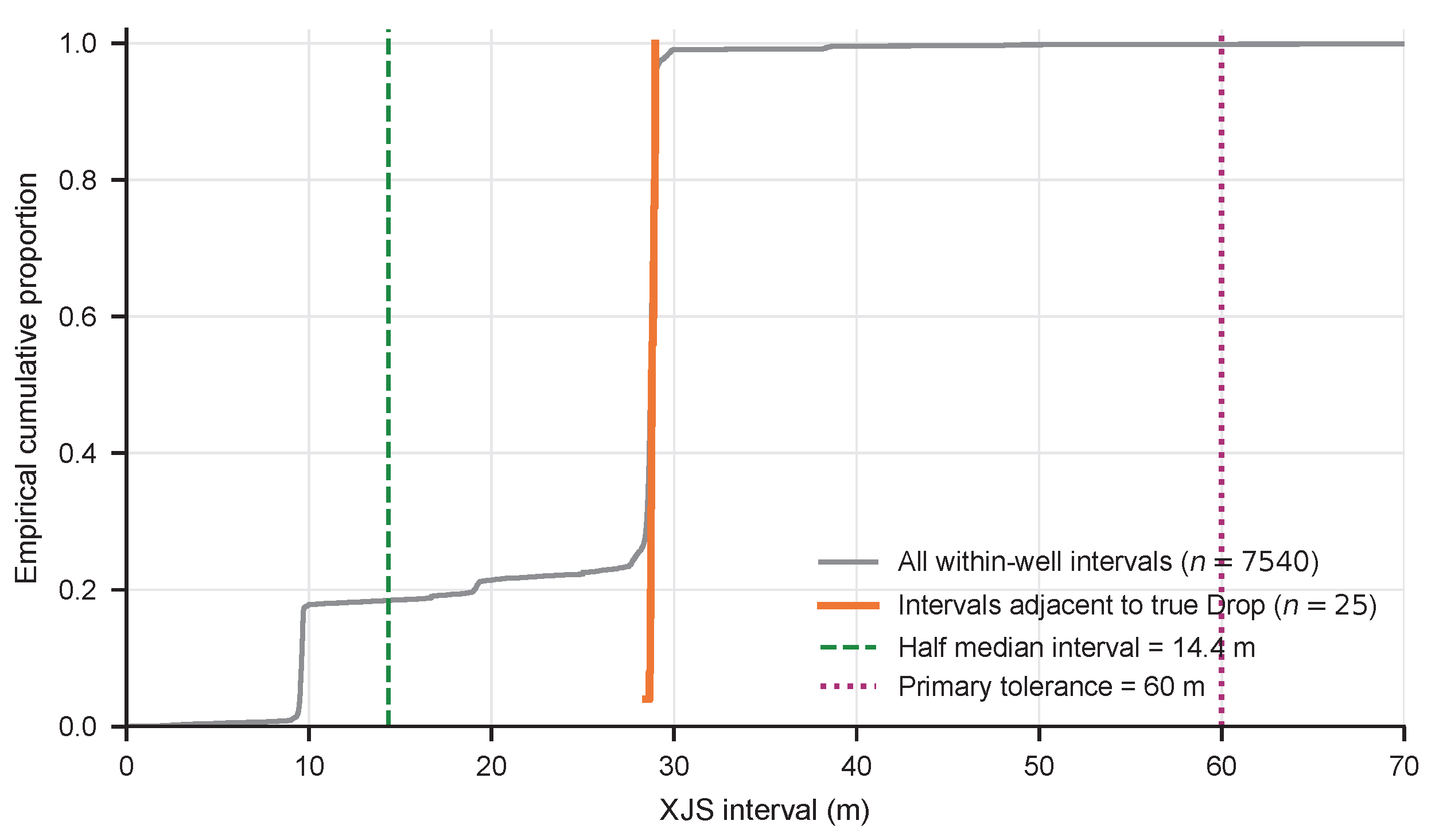
Survey-grid resolution was summarized from all positive within-well XJS intervals and intervals adjacent to labeled Drop stations. The half-median interval was used as a worst-case nearest-station quantization scale, and one quarter of the median interval as the expected absolute error under a uniform within-interval location. These values quantify sampling discretization only because the source file did not provide survey-tool covariance or an ISCWSA error model.

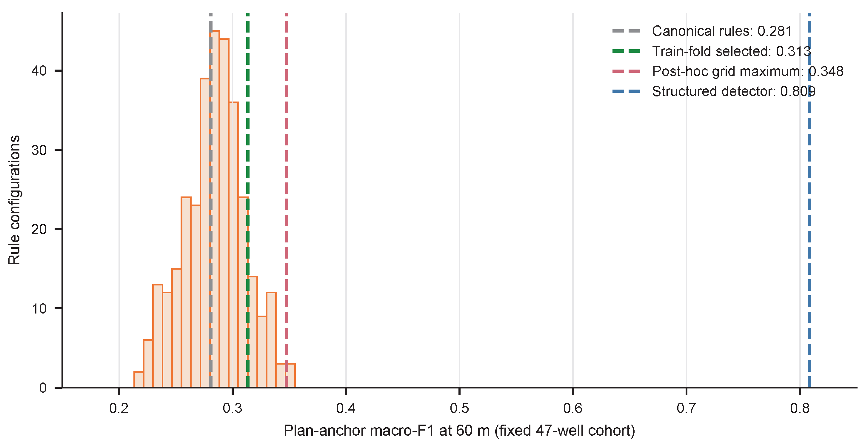
Plan-anchor robustness was evaluated on the fixed 47-well matched cohort across 324 combinations of smoothing window, Build/Hold/Drop slope thresholds, and run length. A nested sensitivity selected a configuration from training wells only in each existing outer fold and applied it to held-out wells. The post-hoc grid maximum was reported only as an optimistic upper bound and was not substituted for the canonical comparator.

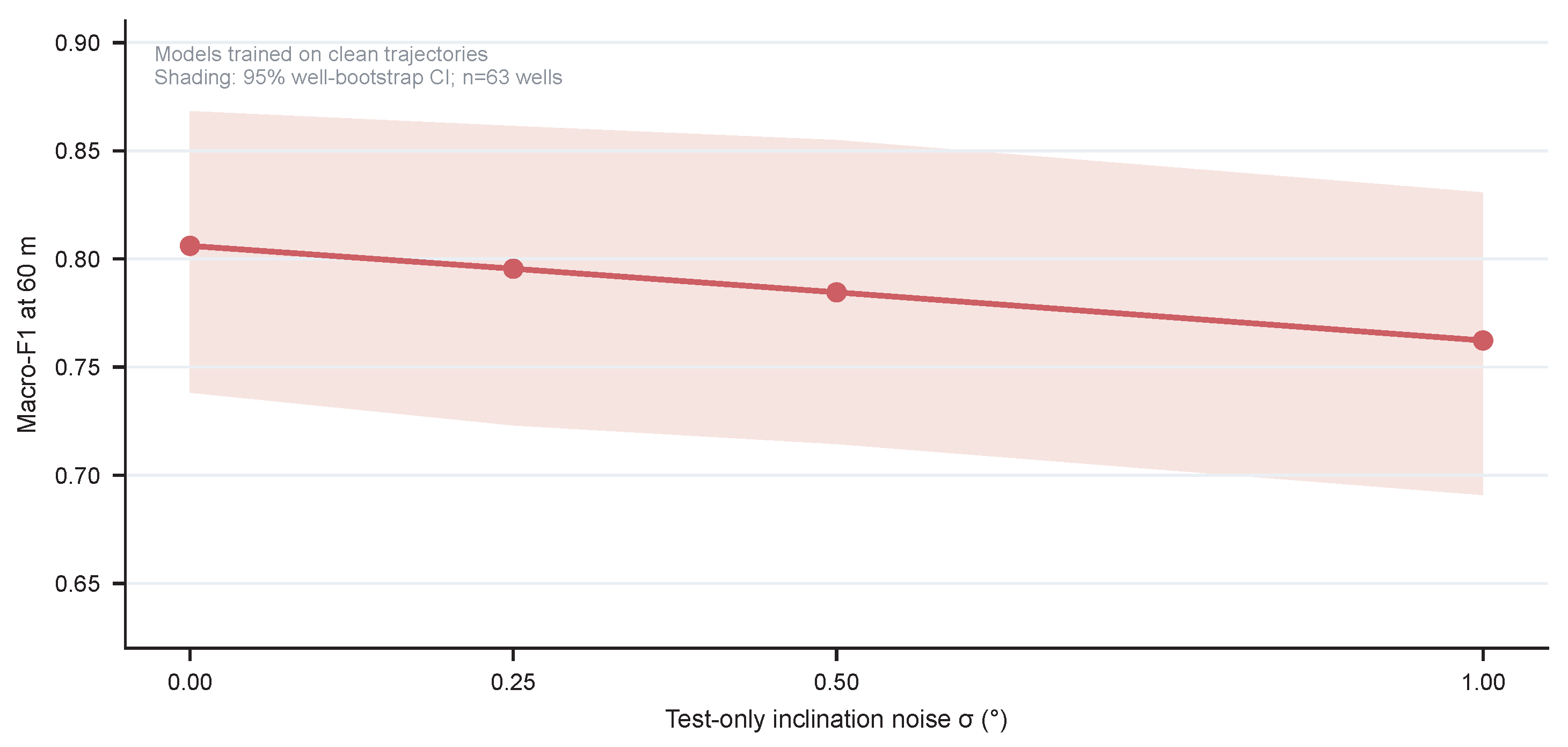
Robustness was assessed by training on clean folds and adding zero-mean Gaussian perturbations with standard deviation 0, 0.25, 0.50, or ${1.00}^{\circ }$ to validation inclination only. Models were not retrained on noisy data. Finally, the excluded build-only well tested the consequence of violating the model’s required Build–Hold scope.

Experiments used Python 3.9.13, NumPy 1.21.5, pandas 1.4.4, SciPy 1.9.1, scikit-learn 1.0.2, and LightGBM 4.6.0. The two trajectory-only baselines required 2.6 and 3.0 s, respectively, for 7603 stations on the analysis workstation. The primary OOF predictions and main performance estimates remained frozen during revision. The added cohort, failure, resolution, and Plan-anchor analyses were derived from those frozen rows; only feature-gain extraction and leave-one-feature-out sensitivity required refitting the original event models under the same folds and settings. Fold assignments, event rows, baseline predictions, paired summaries, and figure source tables are included in the reproducibility package.

4. Results

4.1. Transition Localization

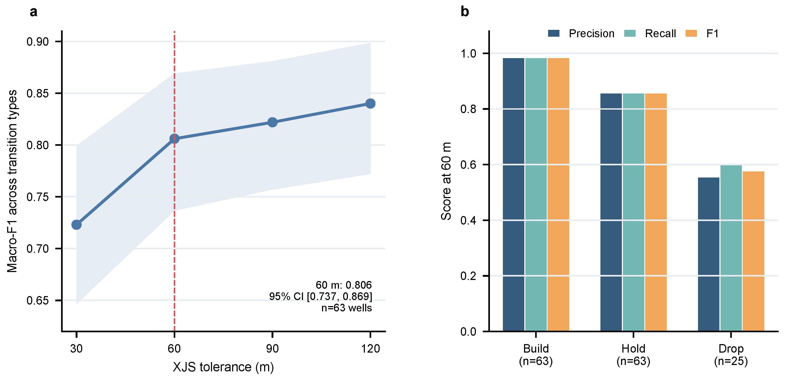
At 60 m, the structured model achieved a macro-F1 of 0.806 (95% CI, 0.737–0.869;

Table 3. Event-level performance at the prespecified 60 m XJS tolerance. Confidence intervals are 2.5th and 97.5th percentiles from 2000 well-bootstrap replicates. The Plan anchor row uses the 47 wells with an extracted planned Build anchor.

Method	Macro-F1	95% CI
Rule based	0.616	0.545–0.688
Change-point DP	0.567	0.509–0.628
Segmented regression	0.615	0.551–0.675
Independent top-one	0.806	0.737–0.869
Greedy ordered	0.806	0.737–0.869
Structured DP	0.806	0.737–0.869
Plan anchor ($n=47$)	0.281	0.200–0.364

; Figure 2a). The point estimate increased from 0.723 at 30 m to 0.840 at 120 m, showing the expected dependence on physical matching tolerance. Confidence intervals remained wide because the independent sample contained 63 wells and only 25 Drop events.

Build was localized most reliably, with precision, recall, and F1 all equal to 0.984 (62 true positives, one false positive, and one false negative). Hold F1 was 0.857 (54/9/9), whereas Drop F1 was 0.577, with precision 0.556 and recall 0.600 (15/12/10; Figure 2b). For paired events, median absolute errors were $0.0$ m for Build (interquartile range, 0.0–9.6; $n=63$), $9.5$ m for Hold (0.0–28.9; $n=63$), and $43.2$ m for Drop (28.6–172.4; $n=22$). The event-level results identify Drop, rather than Build or Hold, as the principal localization limitation.

4.2. Independent Strong-Baseline Comparison

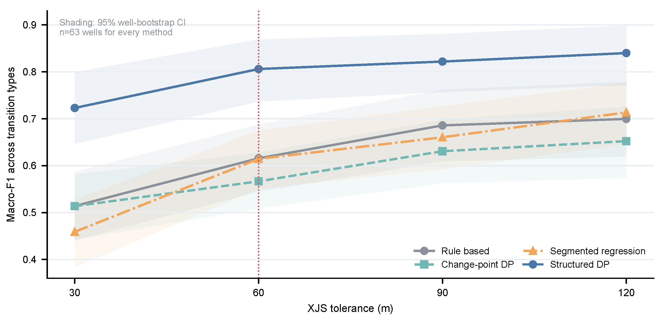
The trajectory-only comparators did not close the performance gap across the evaluated tolerances (Figure 3). At 60 m, change-point dynamic programming achieved a macro-F1 of 0.567 and segmented regression achieved 0.615. The derivative rule remained the strongest observed classical comparator at 0.616, compared with 0.806 for the structured detector. The same ordering persisted at 30, 90, and 120 m, so the comparison was not created by selecting the primary tolerance after inspection.

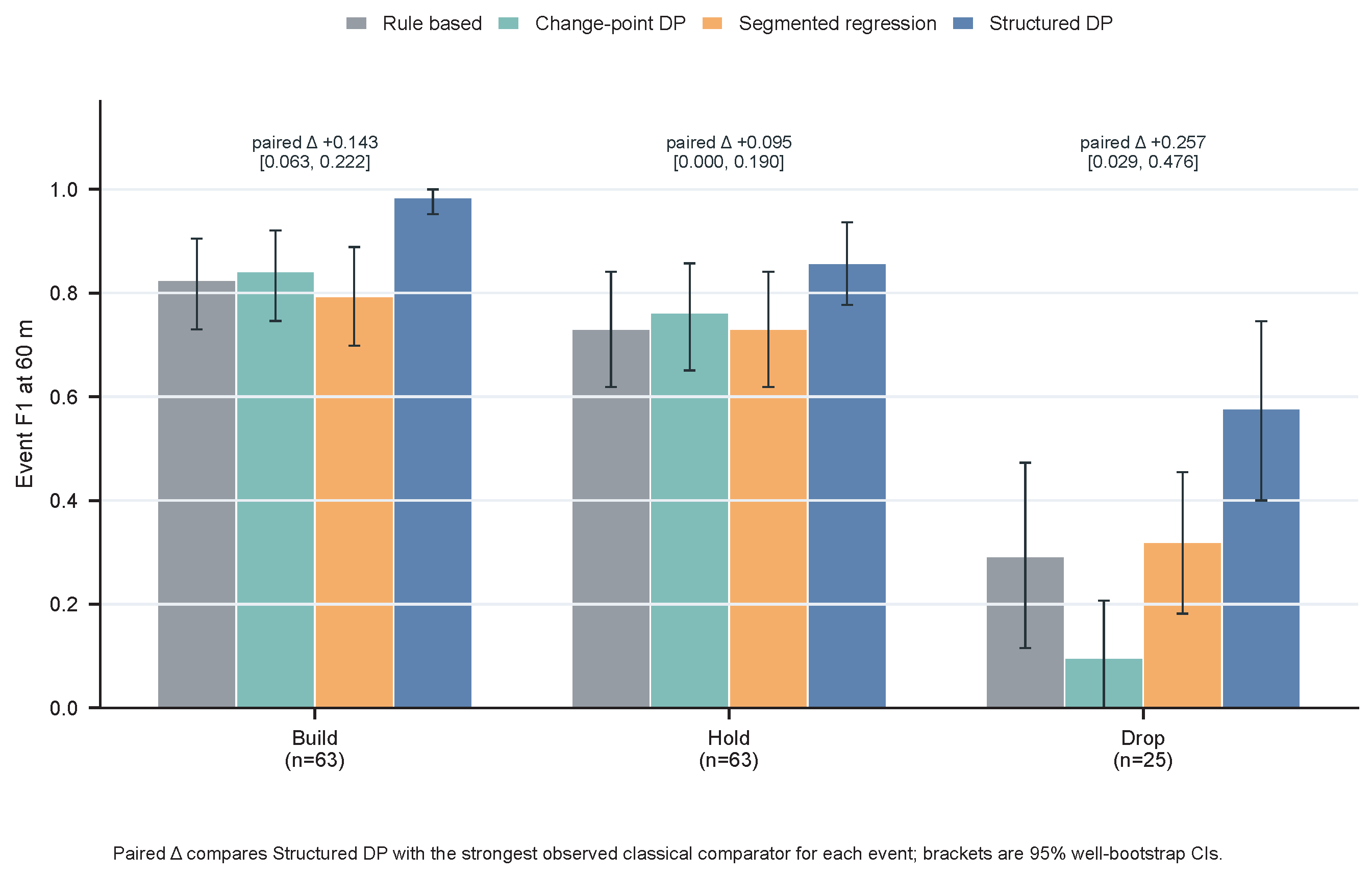
The event-specific comparison separated this aggregate result into its physical transitions (Figure 4). The strongest observed classical comparator was change-point DP for Build and Hold, with F1 values of 0.841 and 0.762, and segmented regression for Drop, with F1 of 0.320. The structured detector achieved 0.984, 0.857, and 0.577, respectively. Paired event-specific differences were 0.143 for Build (95% CI, 0.063–0.222), 0.095 for Hold (0.000–0.190), and 0.257 for Drop (0.029–0.476). Thus, the point estimate favored the structured detector for every event, although the Hold interval reached zero and Drop remained the least accurately localized event for all methods.

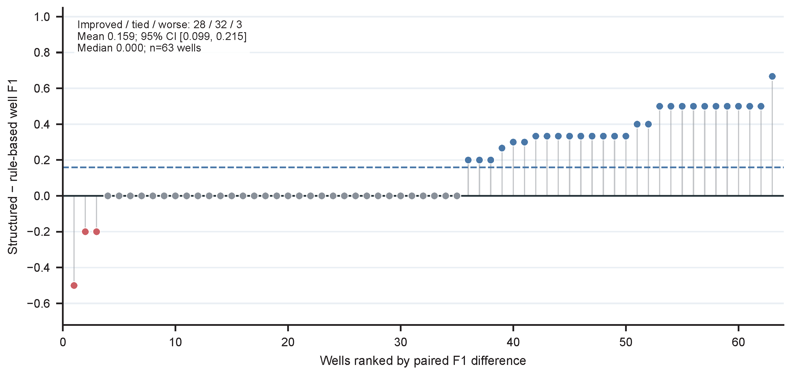
The aggregate paired comparison also remained visible at well level (Figure 5). Structured macro-F1 exceeded the strongest observed classical comparator by 0.190 under paired resampling (95% CI, 0.111–0.268). The mean well-level F1 difference was 0.159 (0.099–0.215): 28 wells improved, 32 tied, and 3 worsened. The zero median therefore reflects the large tied group, not absence of aggregate gain, and the ranked distribution shows that the effect was distributed across multiple improved wells rather than one extreme observation.

4.3. Effect and Current Role of Structured Decoding

Independent top-one, greedy ordered, and structured DP produced identical out-of-fold event locations and macro-F1 values at every tolerance. Their predicted event order was valid in all 63 primary wells, and the paired structured-minus-greedy well-level difference was 0.000 (95% CI, 0.000–0.000). Thus, dynamic programming currently acts only as an explicit validity constraint and reproducible joint objective. This dataset provides no evidence for a joint-decoding accuracy advantage because the learned event scores already peaked in a legal order. Repeated-transition trajectories with competing local maxima are required to test such an advantage. Accordingly, the observed performance difference between the full detector and the classical baselines cannot be attributed to DP; the empirically demonstrated contribution of DP here is enforcement of admissible event order and separation constraints.

4.4. Drop-Presence Identification

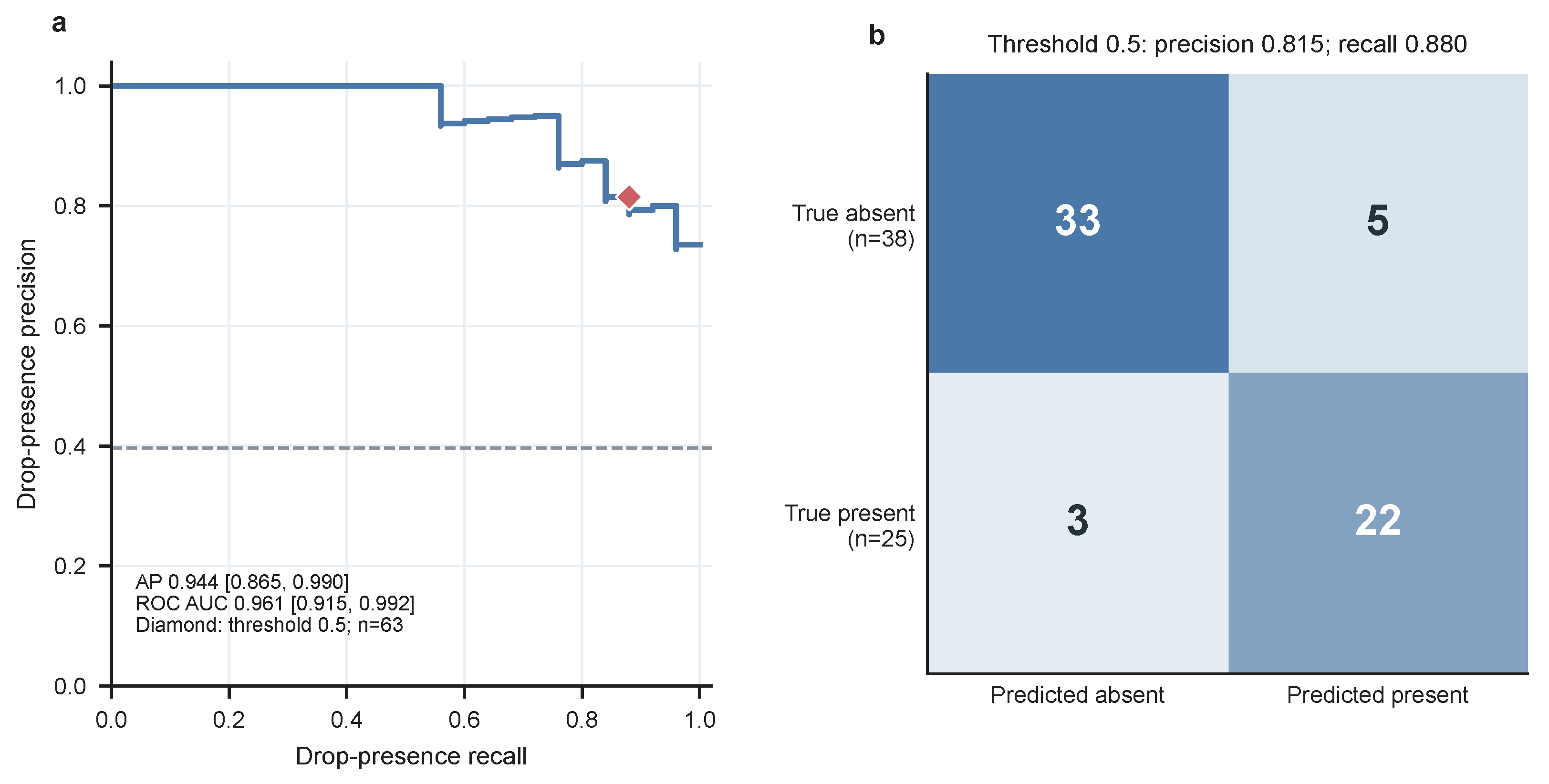
Drop presence was first evaluated independently of event location (Figure 6). Presence achieved a precision of 0.815 (95% CI, 0.652–0.952), recall of 0.880 (0.739–1.000), and specificity of 0.868 (0.757–0.971). Average precision was 0.944 (0.865–0.990), receiver-operating-characteristic area was 0.961 (0.915–0.992), and the Brier score was 0.081 (0.044–0.124). At the prespecified 0.5 threshold, the model identified 22 of 25 Drop wells and produced 5 false-presence decisions among 38 no-Drop wells. A descriptive threshold sweep gave a maximum observed presence F1 of 0.852 at thresholds 0.30–0.45, compared with 0.846 at 0.5; the reported operating point was not retuned.

4.5. Trajectory Characteristics of Drop and No-Drop Wells

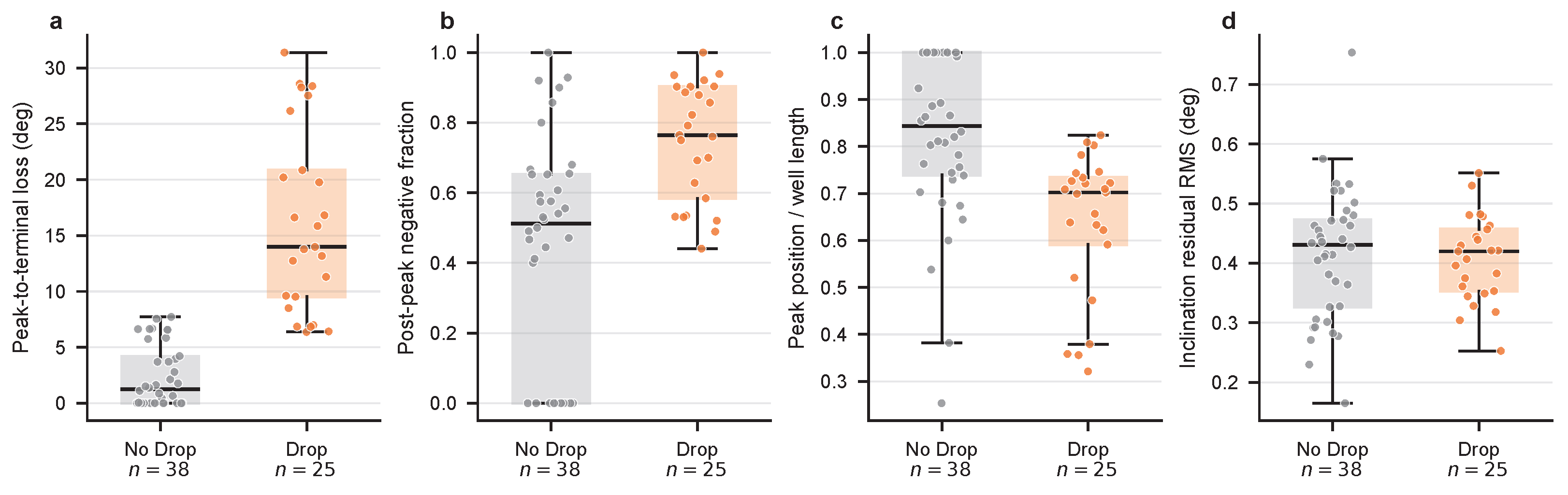
The 25 Drop wells showed substantially larger peak-to-terminal inclination loss than the 38 no-Drop wells: median 13.98° (interquartile range, 9.53–20.85) versus 1.24° (0.00–4.15), with Cliff’s $\delta =0.958$ and Holm-adjusted $p<{10}^{-8}$ (Figure 7a). Their post-peak negative-gradient fraction was also higher, 0.765 versus 0.513 ($\delta =0.565$, adjusted $p=0.000632$), and peak inclination occurred earlier in the normalized trajectory, 0.702 versus 0.843 ($\delta =-0.634$, adjusted $p=0.000114$; Figure 7b,c). Median trajectory length was $3065.0$ m versus $2623.5$ m ($\delta =0.413$, adjusted $p=0.0181$). In contrast, inclination residual RMS was similar, 0.420° versus 0.430° ($\delta =-0.034$, adjusted $p=0.828$; Figure 7d), and the small station-spacing difference did not remain below 0.05 after correction (adjusted $p=0.0568$). The Drop cohort was therefore distinguished mainly by sustained terminal decline and where the inclination peak occurred, rather than by greater residual noise.

4.6. Conditional Drop Localization

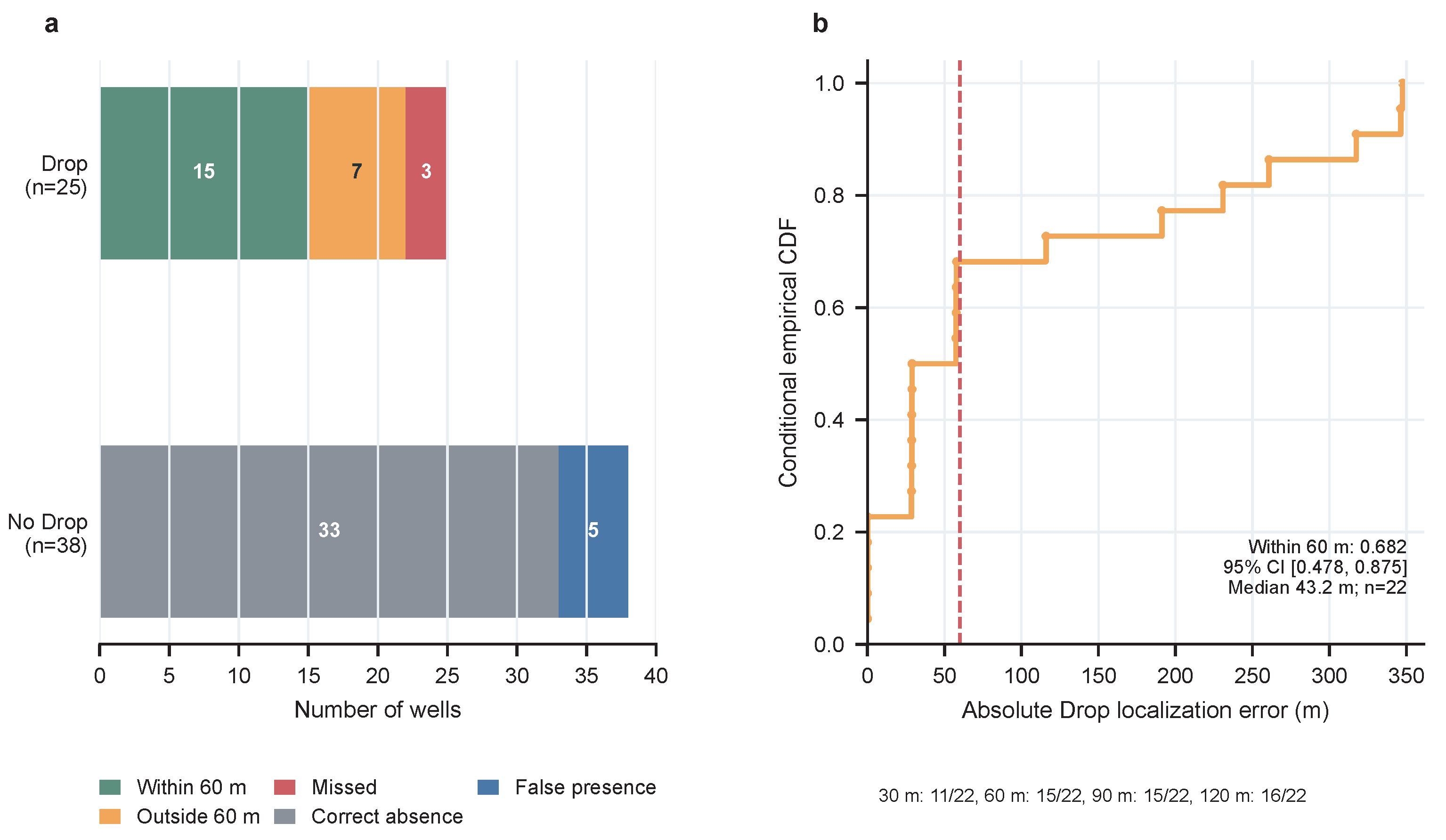
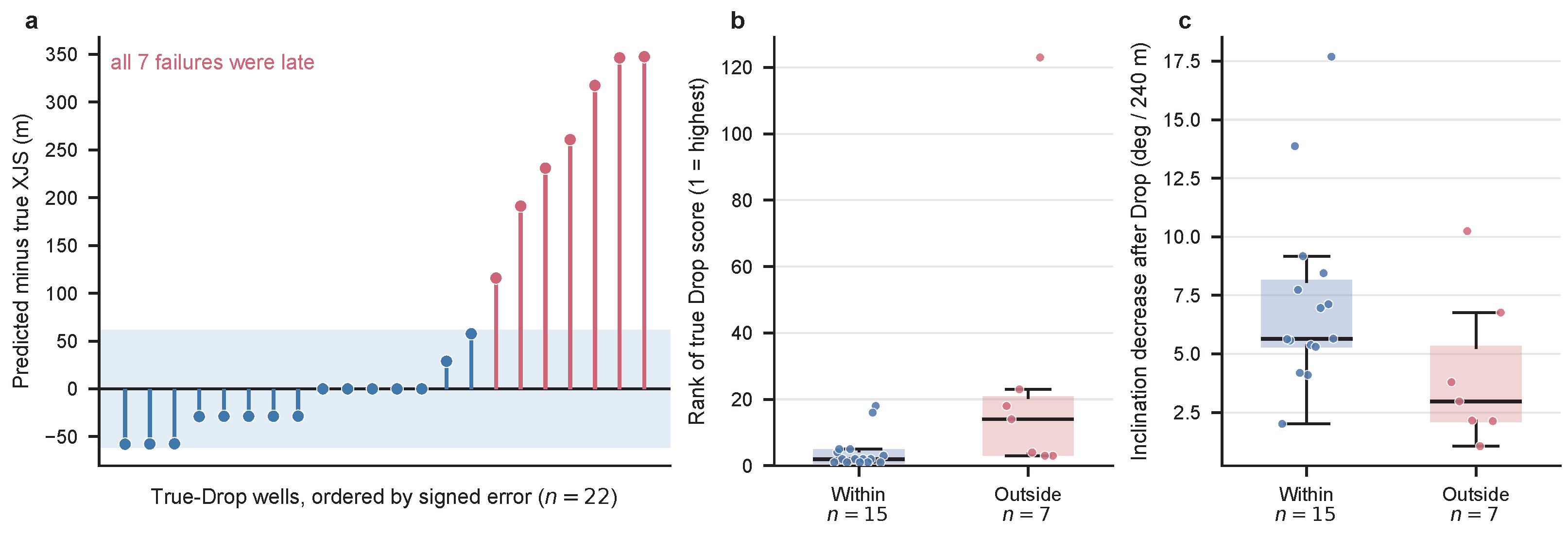
Localization was then evaluated only for the 22 true-Drop wells in which a Drop was emitted (Figure 8). Fifteen were localized within 60 m, whereas seven were outside tolerance. The conditional within-tolerance proportion was 0.682 (95% CI, 0.478–0.875), and the median absolute error was $43.2$ m (28.7–115.9). Within-tolerance counts were 11/22 at 30 m, 15/22 at 60 m, 15/22 at 90 m, and 16/22 at 120 m. The absence of improvement between 60 and 90 m and the single additional match at 120 m show that several residual errors were not marginal threshold misses.

Across all 63 wells, the exhaustive taxonomy comprised 33 correct absences, 5 false presences, 3 missed presences, 15 detections localized within 60 m, and 7 detected Drops outside tolerance. The event-level Drop F1 of 0.577 therefore combined eight presence errors with seven additional localization failures; high presence ranking was not equivalent to usable event localization.

All seven outside-tolerance predictions occurred after the labeled Drop, with signed errors of 115.9–347.5 m and station offsets of 4–12 (Figure 9a). Their median labeled-station score rank was 14, compared with 2 for the 15 within-tolerance detections, whereas the selected late station had a much higher median score than the labeled station (0.363 versus 0.003). The median inclination decrease over the first 240 m after the labeled Drop was also smaller in failures, 2.97° versus 5.65° (Figure 9b,c). Local residual RMS and station spacing were similar in magnitude between groups. These descriptive findings support two interacting failure modes: the initial decline may be weak or gradual, and a later negative-slope segment can then receive the dominant Drop score. The pattern was not universal, so the small seven-well set does not establish a single causal mechanism.

4.7. Survey-Station Resolution and the Localization Floor

Across 7540 positive within-well intervals, the 5th percentile, median, and 95th percentile XJS spacings were 9.52, 28.71, and $29.02$ m, respectively (Figure 10). The median interval adjacent to the 25 labeled Drop stations was $28.78$ m. For an unobserved continuous transition rounded to the nearest station, half the median interval gives a $14.36$ m worst-case discretization scale, while a uniform within-interval assumption gives an expected absolute quantization error of $7.18$ m. The primary 60 m tolerance equals 2.09 median intervals. Because the seven Drop failures spanned 4–12 stations, station discretization alone cannot explain them. These calculations do not include directional-survey position uncertainty, for which tool-specific covariance inputs were unavailable.

4.8. Planned Versus As-Drilled Transitions

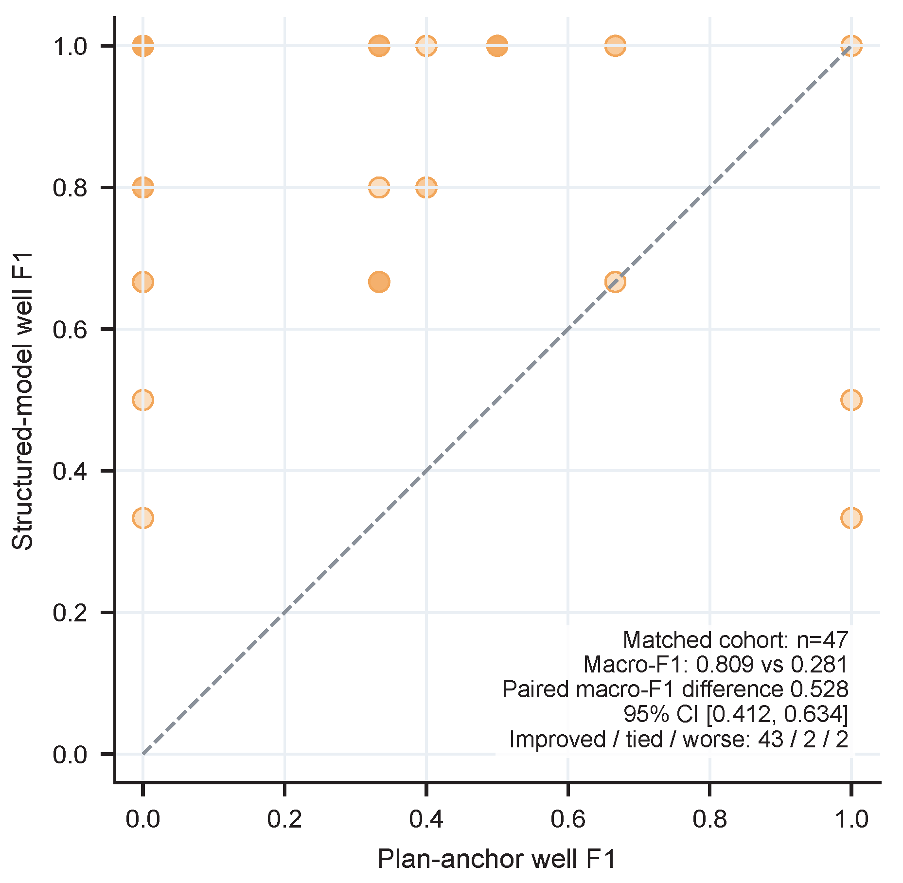
Planned anchors alone gave a 60 m macro-F1 of 0.281 in 47 wells, compared with 0.809 for the detector on the same wells (Figure 11). The paired macro-F1 difference was 0.528 (95% CI, 0.412–0.634). Well-level F1 improved in 43 wells, tied in 2, and worsened in 2. This matched-cohort comparison treats unavailable planned Hold or Drop anchors as missing predictions and shows that design-derived breakpoints were not adequate substitutes for realized transitions.

Across 324 rule configurations, Plan-anchor macro-F1 had a median of 0.284 and a 5th–95th percentile range of 0.233–0.331 on the same 47 wells (Figure 12). Training-fold-only rule selection yielded 0.313 on held-out wells. Even the optimistic post-hoc grid maximum was 0.348, compared with 0.809 for the detector. The canonical result was therefore not explained by one unusually poor heuristic setting, although the increase from 0.281 to 0.313 confirms some threshold sensitivity.

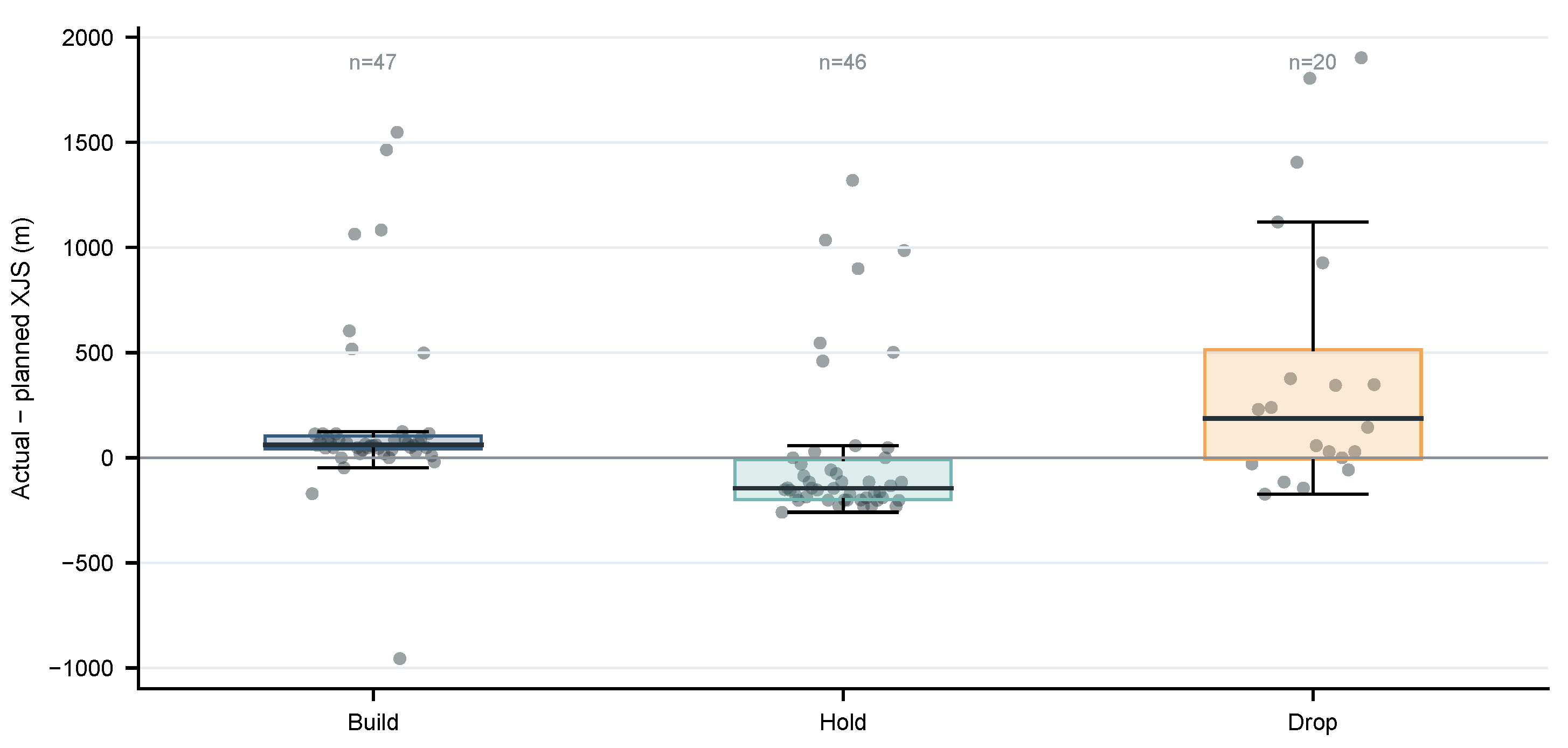
The magnitude and direction of plan–actual offsets differed by event (Figure 13). Among paired planned and organizer-provided events, the median actual-minus-planned offsets were $61.7$ m for Build ($n=47$), $-144.8$ m for Hold ($n=46$), and $187.5$ m for Drop ($n=20$). Their broad distributions show that a single deterministic correction to all plan anchors would not recover the realized events. These offsets combine realized conformance differences with uncertainty from the transparent anchor-extraction rule and should not be interpreted as pure drilling-control error.

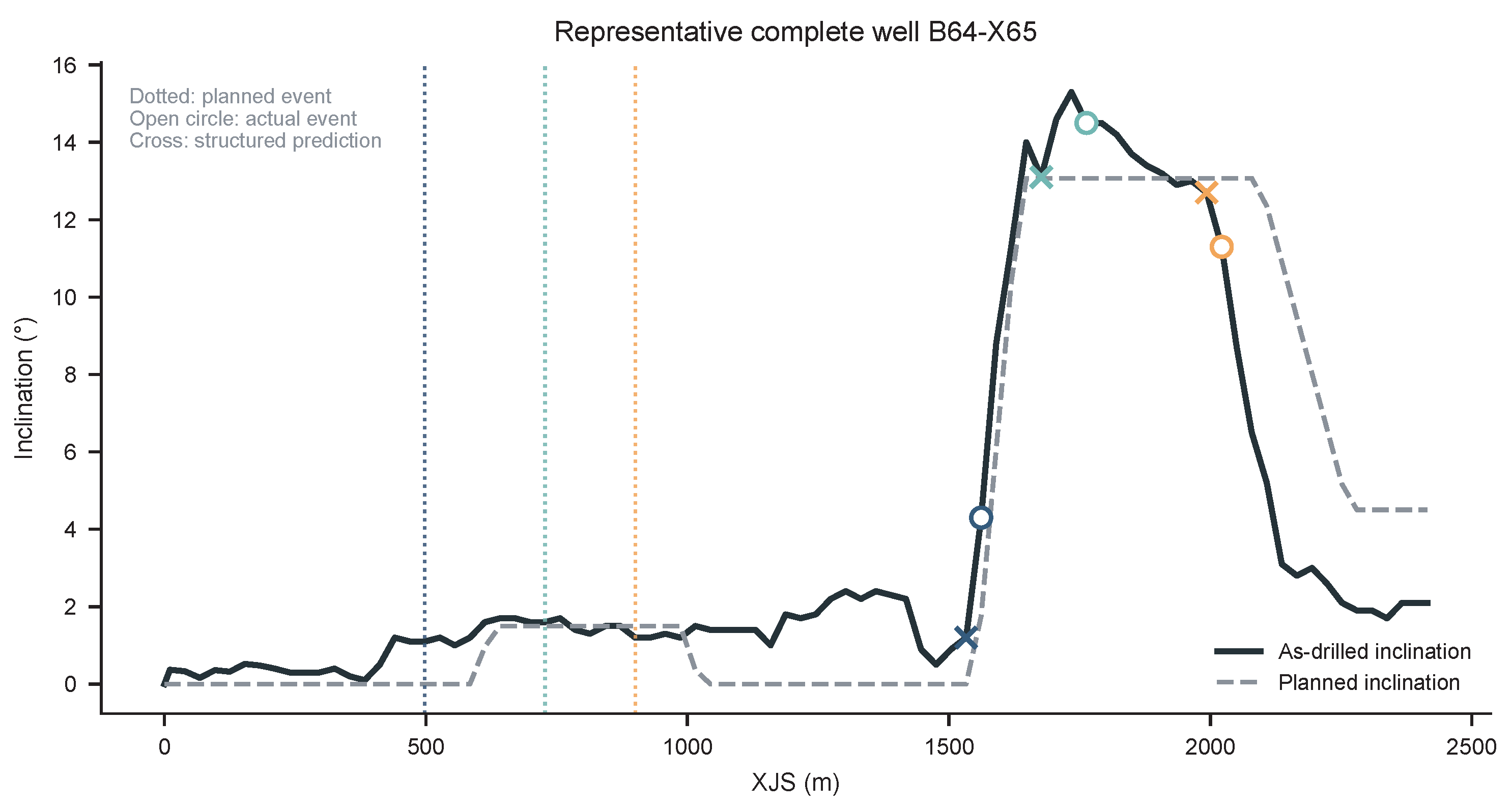
The trace-level distinction is illustrated by B64-X65 (Figure 14), selected deterministically as the complete three-event well whose mean detected-to-actual error was closest to the median among complete cases. Planned, organizer-provided, and detected transitions remain separate records even where the planned and as-drilled inclination shapes have similar large-scale geometry. Retaining all three locations makes the record auditable and permits event-specific conformance review. The candidate set required both labeled and predicted Build, Hold, and Drop events. For each candidate, mean absolute XJS error was calculated across the three events; B64-X65 minimized the absolute difference between this value and the candidate-set median. No visual criterion entered the selection.

4.9. Feature Contribution

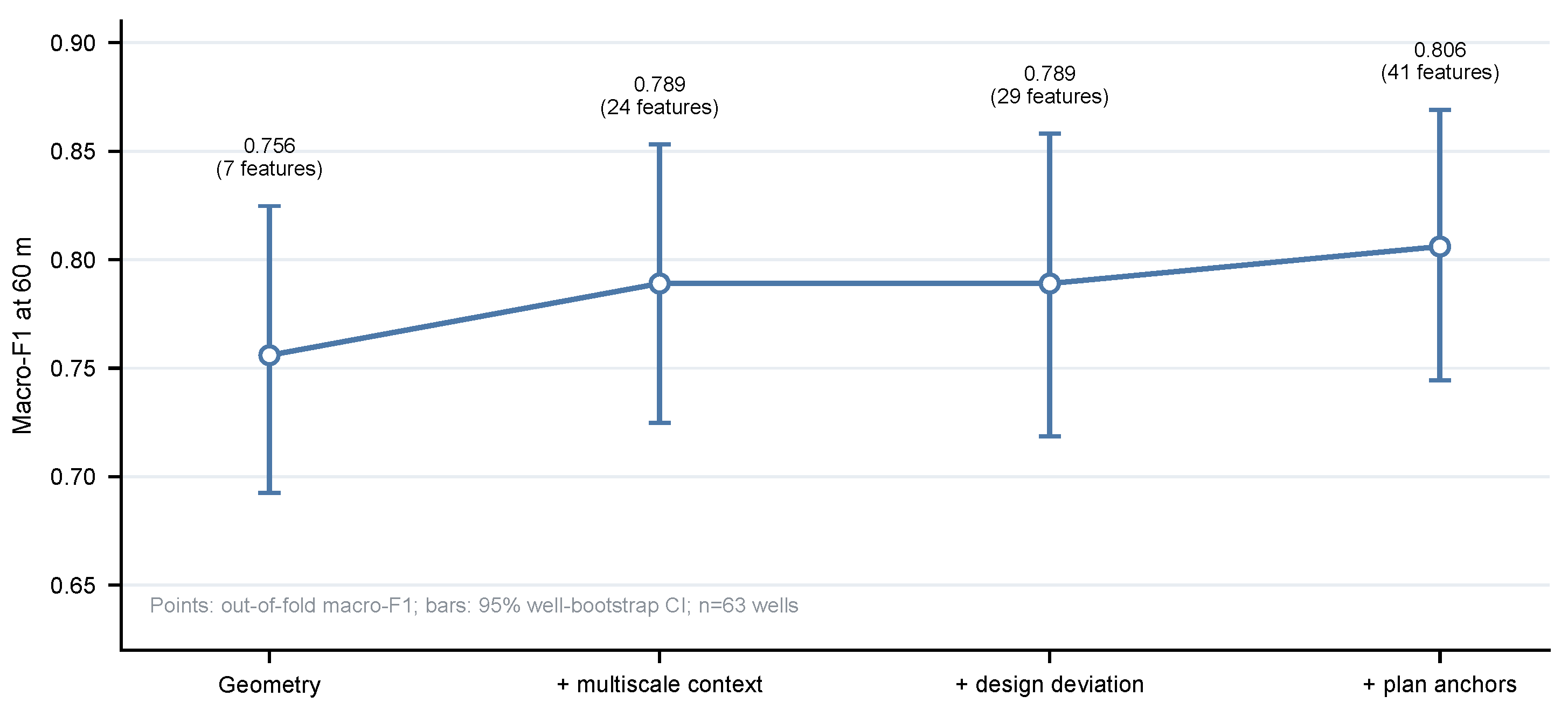
The cumulative feature ablation increased the 60 m macro-F1 point estimate from 0.756 (95% CI, 0.693–0.825) for G1 geometry to 0.789 (0.725–0.853) after multiscale context was added (Figure 15). Adding design-deviation variables did not change the point estimate, whereas planned-anchor features increased it to 0.806 (0.744–0.869). The overlapping intervals preclude a strong claim for either incremental change; the result instead identifies multiscale as-drilled context as the largest observed feature-group increment.

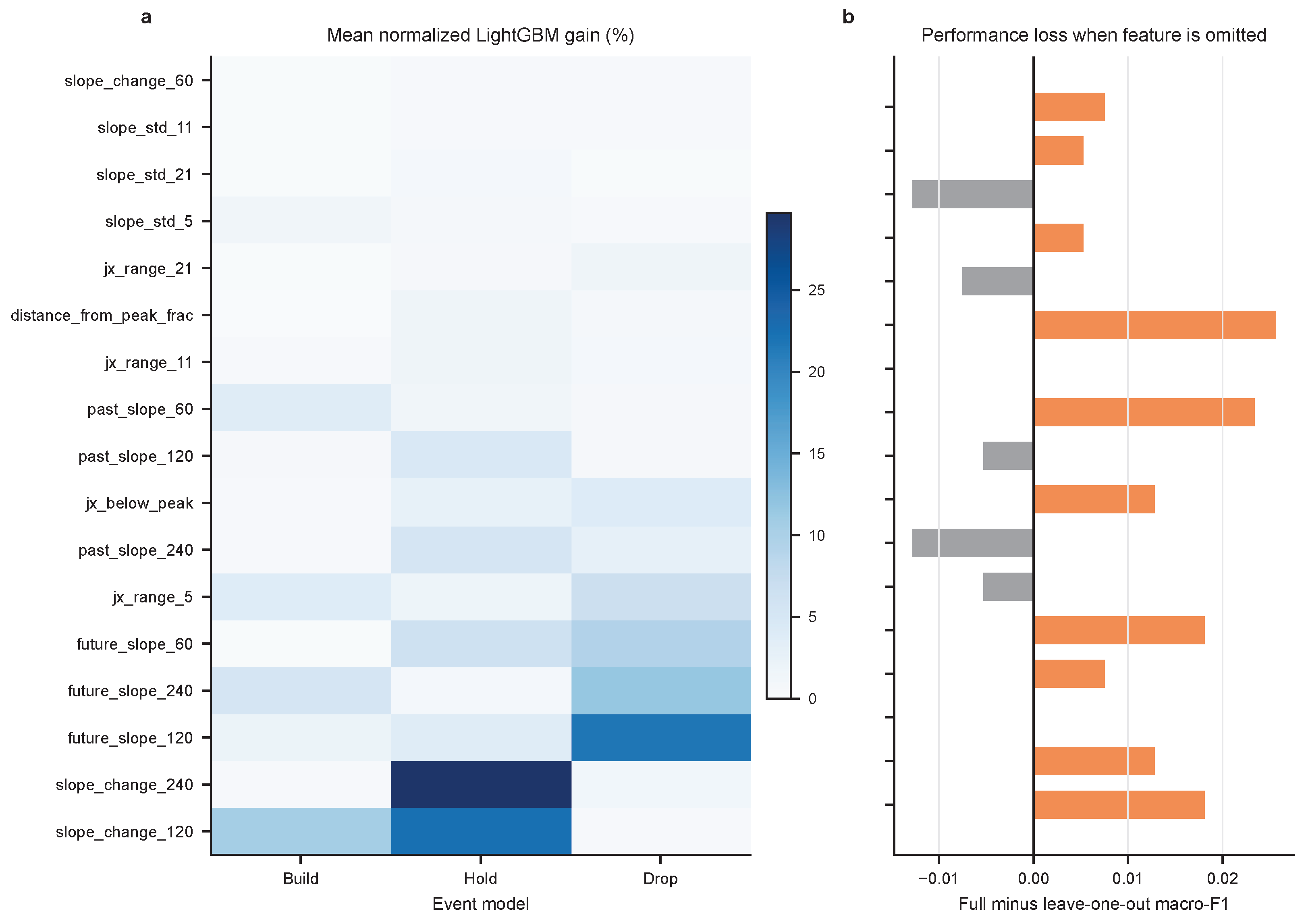
Individual-feature analysis resolved the 17-variable G2 group (Figure 16). Averaged across event models and folds, the leading variables were 120 m slope change (11.1% normalized gain), 240 m slope change (10.4%), and 120 m forward slope (9.0%). The event-specific leaders were 120 m slope change for Build (10.6%), 240 m slope change for Hold (29.7%), and 120 m forward slope for Drop (21.5%). Leave-one-feature-out refitting gave a complementary ranking. Omitting the 5-station inclination range reduced macro-F1 by 0.026, omitting inclination below peak reduced it by 0.023, and omitting either the 60 m slope change or 21-station inclination range reduced it by 0.018. Several high-gain variables caused little loss, and removing three variables slightly increased the point estimate. This disagreement between gain and omission rankings indicates redundancy among correlated multiscale descriptors rather than one indispensable feature.

4.10. Measurement-Perturbation Robustness

Under test-only inclination noise, macro-F1 decreased from 0.806 on clean trajectories to 0.795 at ${0.25}^{\circ }$, 0.785 at ${0.50}^{\circ }$, and 0.762 at ${1.00}^{\circ }$ (Figure 17). The respective confidence intervals overlapped. The monotonic point estimates support gradual degradation within the tested perturbation range, not noise invariance or a precisely estimated degradation rate.

4.11. Scope-Sensitivity Case

The held-out build-only well B509-P13 violated the required Build–Hold scope. After training on all 63 primary wells, the model detected its Build at XJS $735.4$ m, compared with the label at $754.5$ m, but also emitted a false Hold at $1547.2$ m. No Drop was emitted. This is direct evidence that the present state graph should not be applied to build-only, repeated-build, repeated-hold, or seven-section trajectories without adding explicit states and training examples.

5. Discussion

The principal result is not that a design breakpoint can be rediscovered. It is that realized events can be stored separately from planned counterparts under a well-level event protocol. The model exceeded three classical trajectory comparators across all evaluated tolerances, with a paired macro-F1 difference of 0.190 from the strongest observed comparator. Event-specific paired estimates favored the detector for Build, Hold, and Drop, although the Hold interval reached zero. At well level, 28 cases improved, 32 tied, and 3 worsened. The benefit was therefore distributed but not universal, a pattern that is obscured by an aggregate score alone.

The comparison also clarifies how the task differs from generic signal segmentation. Offline change-point methods are designed to partition an ordered signal when the number, type, or location of distributional changes is unknown [25]. Well-log studies have successfully used multivariate changes or learned depth context to identify lithologic boundaries and classes [28,29,30]. Here, by contrast, the targets are a small set of operationally defined trajectory events with a prescribed order and an optional terminal state. The classical change-point and segmented-regression baselines test whether generic piecewise structure is sufficient; their lower event F1 indicates that the engineering event definition and planned–actual alignment add information beyond unconstrained segmentation.

The long-form output remains suitable for audit. Post-well reviewers can inspect early or late regime changes without manually scanning every station. The matched Plan comparison strengthens this use case: 43 of 47 wells improved, whereas only two worsened, when realized-event detection replaced planned anchors as the event record. Detected transitions can also index intervals for later BHA-response analysis and standardize event fields across well databases. This retrospective layer is complementary to inclination prediction [13,14], bit projection and motor-yield advisory [16], and closed-loop trajectory-control research [7,9]; it provides consistent event records with which such prospective systems can subsequently be calibrated or reviewed. At a broader system-management scale, the number of extracting wells has been treated as an optimization variable in distributed hydrolithosphere-process control [38]; that field-scale problem is distinct from the within-well transition-localization task considered here. The BHA use remains prospective because operating channels were not available here.

The Drop decomposition distinguishes a presence problem from a localization problem. The presence model ranked Drop wells well, with average precision of 0.944 and recall of 0.880 at the prespecified threshold. The descriptive threshold sweep showed that 0.5 lay near the observed F1 plateau, so the presence result was not dependent on a sharply tuned cutoff. However, seven of 22 true-presence detections remained outside the primary tolerance, and increasing tolerance from 60 to 90 m recovered no additional event. All seven errors were late by 115.9–347.5 m (4–12 survey stations). In these wells, the labeled station typically had a low Drop-score rank and the first 240 m after the label showed a smaller inclination decrease than in successfully localized wells. The detector therefore appears vulnerable when the annotated onset is a weak or gradual decline and a later, steeper negative-slope interval provides stronger evidence. Similar local noise and station spacing between the two groups argue against either factor as the sole explanation. These are descriptive associations from seven failures, not a causal model, but they identify score calibration around gradual onsets as the most direct target for improvement. Presence discrimination is therefore not equivalent to usable event localization, and the 25 Drop wells limit both training diversity and the precision of these estimates.

The structured component should be interpreted narrowly. Equations (3) and (4) guarantee the declared state order, but this guarantee did not alter any out-of-fold prediction relative to greedy selection. Dynamic programming therefore acted only as a validity constraint on this dataset, and claiming a decoding-accuracy gain would be unsupported. A likely explanation is that single-cycle conventional trajectories already provide strong local cues and large event separations. Repeated build/hold cycles may create the competing local maxima needed for joint decoding to matter, but those trajectories were absent from the dataset. Accordingly, the structured component should be understood as a deterministic validity mechanism, not as the source of the detector’s observed localization advantage.

Several limitations define the boundary of the study. The data came from one competition-supplied field collection and contained only 63 primary-scope wells. All reported performance estimates therefore characterize within-dataset out-of-fold performance; they do not establish external generalization across independent fields or acquisition settings. The classical comparators strengthen internal benchmarking but do not replace independent multi-field validation. This concern is material because drilling anomaly models and well-log classifiers can exploit field-specific distributions and depth context [24,29,30]. The organizer-provided event labels were not accompanied by annotator identities, an adjudication protocol, or repeated ratings; inter-rater agreement and label-location uncertainty could therefore not be quantified. This is especially relevant for a gradual Drop onset, where several neighboring stations may be operationally plausible.

Planned anchors used transparent slope heuristics rather than manually optimized per-well rules, and their offsets include anchor-extraction uncertainty. The 324-configuration sensitivity analysis and training-fold-only selection improved Plan-anchor macro-F1 only modestly and did not approach the detector, which reduces—but does not eliminate—the possibility that the canonical anchor rule was suboptimal. More generally, planning under geological uncertainty makes even an optimized target path conditional on the available subsurface realization [19]. Survey uncertainty also extends beyond sampling resolution: wellbore-positioning standards distinguish instrument, depth, magnetic, and propagation errors [10,11,12], whereas this dataset supplied no tool-specific covariance model. The observed median station interval implies an expected nearest-station quantization error near $7.18$ m and a half-interval scale of $14.36$ m; this is well below the 60 m tolerance and cannot explain errors spanning 4–12 stations. The offline features use forward and full-well context and cannot support an online claim. Finally, the build-only case shows that a fixed Build–Hold graph emits a structurally predictable false event when its scope assumption is violated.

Future work should extend the state graph to repeated Build, Hold, Drop, tangent, and correction sections; collect multi-field wells with independent expert annotations; represent transition locations as intervals or probability distributions; and test resolution-aware objectives that do not over-penalize adjacent plausible stations. Joint decoding should then be re-evaluated on multi-cycle trajectories containing genuinely competing event candidates. Linking the standardized event table to BHA, weight-on-bit, rotary speed, and steering-command records is also required before causal BHA-response hypotheses or streaming-control applications can be tested.

6. Conclusions

This study formulated post-well trajectory assessment as well-level localization of actual Build, Hold, and optional Drop events. Across 63 primary-scope wells, the detector achieved a 60 m macro-F1 of 0.806 and exceeded three classical trajectory comparators across the tested tolerances. Paired event and well analyses showed where this advantage occurred and where ties remained. Drop presence was identified more reliably than Drop location, and the seven late localization failures were associated with weak early decline and low labeled-station score rank. Planned anchors were not adequate substitutes for realized events, including under rule-sensitivity analysis. Exact dynamic programming guaranteed a legal output sequence but did not improve localization over greedy decoding. Within the evaluated dataset, the results support the feasibility of bounded offline assessment of completed trajectories containing exactly one Build, exactly one Hold, and at most one Drop. Build-only, repeated-transition, multi-Build/multi-Hold, seven-section, and real-time trajectories require an extended state graph and new validation data. The reported estimates establish within-dataset out-of-fold performance only; external multi-field generalization remains untested and requires independent validation.

References

1. Ma, T.; Chen, P.; Zhao, J. Overview on vertical and directional drilling technologies for the exploration and exploitation of deep petroleum resources. Geomech. Geophys. Geo-Energy Geo-Resour. 2016, 2, 365–395. [Google Scholar] [CrossRef] [Scilit]
2. Downton, G.C. Systems Modeling and Design of Automated-Directional-Drilling Systems. SPE Drill. Complet. 2015, 30, 212–232. [Google Scholar] [CrossRef] [Scilit]
3. Kristoffersen, B.S.; Bellout, M.C.; Silva, T.L.; Berg, C.F. An Automatic Well Planner for Complex Well Trajectories. Math. Geosci. 2021, 53, 1881–1905. [Google Scholar] [CrossRef] [Scilit]
4. Liu, S.j.; Zhou, X.m.; Zhang, J.w.; Xie, Z.d. The optimization algorithm for application in directional drilling trajectories of energy field. Energy Rep. 2022, 8, 1212–1217. [Google Scholar] [CrossRef] [Scilit]
5. Gulyayev, V.I.; Glazunov, S.N.; Andrusenko, E.N. Optimal control of deep petroleum borehole trajectory tracking. Upstream Oil Gas Technol. 2021, 7, 100049. [Google Scholar] [CrossRef] [Scilit]
6. Cai, Z.; Lai, X.; Wu, M.; Chen, L.; Lu, C. Observer-based trajectory control for directional drilling process. Asian J. Control 2022, 24, 259–272. [Google Scholar] [CrossRef] [Scilit]
7. Cai, Z.; Lai, X.; Wu, M.; Lu, C.; Chen, L. Equivalent-input-disturbance-based robust control of drilling trajectory with weight-on-bit uncertainty in directional drilling. ISA Trans. 2022, 127, 370–382. [Google Scholar] [CrossRef] [Scilit] [PubMed]
8. Zhang, D.; Wu, M.; Lu, C.; Chen, L.; Cao, W. A deviation correction strategy based on particle filtering and improved model predictive control for vertical drilling. ISA Trans. 2021, 111, 265–274. [Google Scholar] [CrossRef] [Scilit] [PubMed]
9. Hao, J.; You, Q.; Peng, Z.; Ma, D.; Tian, Y. A model-free toolface control strategy for cross-well intelligent directional drilling. Eng. Appl. Artif. Intell. 2024, 133, 108272. [Google Scholar] [CrossRef] [Scilit]
10. Williamson, H.S. Accuracy Prediction for Directional Measurement While Drilling. SPE Drill. Complet. 2000, 15, 221–233. [Google Scholar] [CrossRef] [Scilit]
11. ISCWSA Error Model Maintenance Group. Definition of the ISCWSA Error Model: Revision 4.3. 2017. Available online: https://www.iscwsa.net/articles/definition-of-the-iscwsa-error-model-revision-43/ (accessed on 9 September 2026).
12. Sawaryn, S.J.; Thorogood, J.L. A Compendium of Directional Calculations Based on the Minimum Curvature Method. SPE Drill. Complet. 2005, 20, 24–36. [Google Scholar] [CrossRef] [Scilit]
13. Tunkiel, A.T.; Sui, D.; Wiktorski, T. Training-while-drilling approach to inclination prediction in directional drilling utilizing recurrent neural networks. J. Pet. Sci. Eng. 2021, 196, 108128. [Google Scholar] [CrossRef] [Scilit]
14. Yan, B.; Zhang, X.; Tang, C.; Wang, X.; Yang, Y.; Xu, W. A Random Forest-Based Method for Predicting Borehole Trajectories. Mathematics 2023, 11, 1297. [Google Scholar] [CrossRef] [Scilit]
15. Keller, A.M.; Feng, T.; Demirer, N.; Darbe, R.; Chen, D. Rate of penetration estimation downhole with machine learning for drilling position control. Geoenergy Sci. Eng. 2023, 224, 211593. [Google Scholar] [CrossRef] [Scilit]
16. Zhang, Y.; Cao, D.; Chu, J.; Ashok, P.; Chen, D.; van Oort, E.; Harclerode, B.; Vora, K. A data-driven bit projection system with motor yield prediction and advisory for directional drilling and well trajectory control. Geoenergy Sci. Eng. 2024, 239, 212987. [Google Scholar] [CrossRef] [Scilit]
17. Cao, J.; Chowdhury, S.E.; Wiktorski, T.; Sui, D. Well Path Design Using Q-Learning Algorithms and Bezier Curves With Obstacles Avoidance. In Proceedings of the ASME 2022 41st International Conference on Ocean, Offshore and Arctic Engineering, Hamburg, Germany, 5–10 June 2022; p. V010T11A007. [Google Scholar] [CrossRef] [Scilit]
18. Wang, Z.; Shen, S.L.; Chen, D.; Li, W.; Li, W.; Fan, Z. Multi-objective optimization of the wellbore trajectory considering both geological and engineering factors. Geoenergy Sci. Eng. 2025, 246, 213647. [Google Scholar] [CrossRef] [Scilit]
19. Kristoffersen, B.S.; Silva, T.L.; Bellout, M.C.; Berg, C.F. Efficient well placement optimization under uncertainty using a virtual drilling procedure. Comput. Geosci. 2022, 26, 739–756. [Google Scholar] [CrossRef] [Scilit]
20. Saavedra Jerez, L.; Cayeux, E.; Sui, D. Automatic calibration of systematic biases in directional drilling control for planar and non-planar curves. Geoenergy Sci. Eng. 2025, 246, 213642. [Google Scholar] [CrossRef] [Scilit]
21. Barbosa, L.F.F.M.; Nascimento, A.; Mathias, M.H.; de Carvalho, J.A. Machine learning methods applied to drilling rate of penetration prediction and optimization—A review. J. Pet. Sci. Eng. 2019, 183, 106332. [Google Scholar] [CrossRef] [Scilit]
22. Chen, X.; Du, X.; Weng, C.; Yang, J.; Gao, D.; Su, D.; Wang, G. A real-time drilling parameters optimization method for offshore large-scale cluster extended reach drilling based on intelligent optimization algorithm and machine learning. Ocean Eng. 2024, 291, 116375. [Google Scholar] [CrossRef] [Scilit]
23. Brankovic, A.; Matteucci, M.; Restelli, M.; Ferrarini, L.; Piroddi, L.; Spelta, A.; Zausa, F. Data-driven indicators for the detection and prediction of stuck-pipe events in oil&gas drilling operations. Upstream Oil Gas Technol. 2021, 7, 100043. [Google Scholar] [CrossRef] [Scilit]
24. Altindal, M.C.; Nivlet, P.; Tabib, M.; Rasheed, A.; Kristiansen, T.G.; Khosravanian, R. Anomaly detection in multivariate time series of drilling data. Geoenergy Sci. Eng. 2024, 237, 212778. [Google Scholar] [CrossRef] [Scilit]
25. Truong, C.; Oudre, L.; Vayatis, N. Selective review of offline change point detection methods. Signal Process. 2020, 167, 107299. [Google Scholar] [CrossRef] [Scilit]
26. Pang, G.; Shen, C.; Cao, L.; van den Hengel, A. Deep Learning for Anomaly Detection: A Review. ACM Comput. Surv. 2021, 54, 1–38. [Google Scholar] [CrossRef] [Scilit]
27. Blázquez-García, A.; Conde, A.; Mori, U.; Lozano, J.A. A Review on Outlier/Anomaly Detection in Time Series Data. ACM Comput. Surv. 2021, 54, 1–33. [Google Scholar] [CrossRef] [Scilit]
28. Datta, D.; Singh, G.; Singh, S.K.; Jenamani, M.; Routray, A. Application of multivariate change detection in automated lithofacies classification from well-log data in a nonstationary subsurface. J. Appl. Geophys. 2023, 215, 105094. [Google Scholar] [CrossRef] [Scilit]
29. Dong, S.Q.; Zhong, Z.H.; Cui, X.H.; Zeng, L.B.; Yang, X.; Liu, J.J.; Sun, Y.M.; Hao, J.R. A deep kernel method for lithofacies identification using conventional well logs. Pet. Sci. 2023, 20, 1411–1428. [Google Scholar] [CrossRef] [Scilit]
30. Pang, Q.; Chen, C.; Sun, Y.; Pang, S. STNet: Advancing Lithology Identification with a Spatiotemporal Deep Learning Framework for Well Logging Data. Nat. Resour. Res. 2025, 34, 327–350. [Google Scholar] [CrossRef] [Scilit]
31. Sharma, A.; Zhang, J.; Spagnoli, G.; Huang, Z.; Lu, M.; Yao, H.; Wu, S. Fast Semiautomatic Change Point Detection in Deformation Monitoring Using Kullback–Leibler Divergence. ASCE-ASME J. Risk Uncertain. Eng. Syst. Part A Civ. Eng. 2025, 11, 04025057. [Google Scholar] [CrossRef] [Scilit]
32. Cai, W.; Ding, J.; Li, Z.; Yin, Z.; Feng, Y. Study on Rock Mechanics Parameter Prediction Method Based on DTW Similarity and Machine-Learning Algorithms. Petrophysics 2024, 65, 128–144. [Google Scholar] [CrossRef] [Scilit]
33. Savitzky, A.; Golay, M.J.E. Smoothing and Differentiation of Data by Simplified Least Squares Procedures. Anal. Chem. 1964, 36, 1627–1639. [Google Scholar] [CrossRef] [Scilit]
34. Ke, G.; Meng, Q.; Finley, T.; Wang, T.; Chen, W.; Ma, W.; Ye, Q.; Liu, T.Y. LightGBM: A Highly Efficient Gradient Boosting Decision Tree. In Proceedings of the Advances in Neural Information Processing Systems; Curran Associates Inc.: Red Hook, NY, USA, 2017; Volume 30, pp. 3146–3154. [Google Scholar]
35. Bai, J.; Perron, P. Computation and Analysis of Multiple Structural Change Models. J. Appl. Econom. 2003, 18, 1–22. [Google Scholar] [CrossRef] [Scilit]
36. Muggeo, V.M.R. Estimating Regression Models with Unknown Break-Points. Stat. Med. 2003, 22, 3055–3071. [Google Scholar] [CrossRef] [Scilit] [PubMed]
37. Efron, B. Bootstrap Methods: Another Look at the Jackknife. Ann. Stat. 1979, 7, 1–26. [Google Scholar] [CrossRef] [Scilit]
38. Pershin, I.M.; Pervukhin, D.A.; Ilyushin, Y.V.; Afanaseva, O.V. Design of Distributed Systems of Hydrolithosphere Processes Management. Selection of Optimal Number of Extracting Wells. IOP Conf. Ser. Earth Environ. Sci. 2017, 87, 032030. [Google Scholar] [CrossRef] [Scilit]
Figure 1. Workflow for offline transition detection and conformance assessment. Planned stations, the completed as-drilled trajectory, and organizer-provided event labels are aligned in XJS. Domain-informed multiscale descriptors, design deviations, and plan-anchor distances produce event likelihoods. An exact dynamic program returns either a Build–Hold or Build–Hold–Drop sequence. The output is an auditable well-level record of actual transition locations, plan–actual offsets, standardized event fields, and intervals that may later be linked to separately collected BHA records.
Energies 19 04386 g001
Figure 2. Primary transition-localization performance. (a) Structured-model macro-F1 across four XJS tolerances. The dashed line marks the prespecified 60 m tolerance; shading denotes 95% confidence intervals from 2000 well-bootstrap replicates, with wells as the independent unit. (b) Event-specific precision, recall, and F1 at 60 m; n denotes wells containing the true event. Background stations are excluded from all metrics.
Energies 19 04386 g002
Figure 3. Tolerance-dependent comparison with independent trajectory baselines. Macro-F1 is shown at four XJS tolerances for the structured detector and three classical comparators. Shading denotes 95% confidence intervals from 2000 well-bootstrap replicates; all methods were evaluated on the same 63 wells. The vertical dotted line marks the prespecified 60 m tolerance.
Energies 19 04386 g003
Figure 4. Event-specific comparison with classical trajectory baselines. Bars show Build, Hold, and Drop F1 at the prespecified 60 m tolerance; error bars are 95% confidence intervals from 2000 well-bootstrap replicates. n under each event denotes wells containing that true event. The annotation above each event gives the paired F1 difference between the structured detector and the strongest observed classical comparator for that event, with its paired well-bootstrap confidence interval.
Energies 19 04386 g004
Figure 5. Well-level paired advantage over the strongest observed classical comparator. Each point is one well, ranked by the difference between structured and rule-based well F1 at 60 m; stems terminate at zero. Blue, grey, and red denote improved, tied, and worse wells, respectively. The dashed line is the mean difference. The annotation reports the improved/tied/worse counts and the mean 95% confidence interval from 2000 paired well-bootstrap replicates.
Energies 19 04386 g005
Figure 6. Well-level Drop-presence identification. (a) Out-of-fold precision–recall curve across 63 wells. The horizontal dashed line is the observed Drop prevalence (25/63), and the diamond marks the prespecified probability threshold of 0.5. AP denotes average precision; brackets show 95% confidence intervals from 2000 well-bootstrap replicates. (b) Presence confusion matrix at threshold 0.5. Counts use one out-of-fold probability per independent well and do not include localization tolerance.
Energies 19 04386 g006
Figure 7. Well-level characteristics of Drop and no-Drop trajectories. (a) Peak-to-terminal inclination loss. (b) Fraction of post-peak stations with gradient below 0.04 per 30 m. (c) Peak position normalized by station sequence length. (d) Root-mean-square residual between measured and smoothed inclination. Points are independent wells; boxes show the interquartile range, centre lines show medians, and whiskers extend to 1.5 times the interquartile range. Statistical comparisons used two-sided Mann–Whitney tests with Holm adjustment across six descriptors; effect sizes are reported in the text.
Energies 19 04386 g007
Figure 8. Conditional Drop-localization error. (a), Exhaustive outcome categories for all 25 true-Drop and 38 no-Drop wells. Presence errors and localization-outside-tolerance errors are shown separately. Green, orange, red, grey, and blue denote within-tolerance localization, outside-tolerance localization, missed presence, correct absence, and false presence, respectively. (b), Conditional empirical cumulative distribution of absolute Drop localization error in the 22 true-Drop wells where a Drop was emitted. The orange curve shows the empirical distribution, and the red dashed line marks the primary 60 m tolerance; the footer gives within-tolerance counts at all evaluated tolerances. The conditional denominator is fixed at 22 wells.
Energies 19 04386 g008
Figure 9. Diagnostic characterization of the seven Drop localization failures. (a) Signed XJS error for the 22 true-Drop wells in which a Drop was emitted; blue denotes detections within 60 m, red denotes detections outside 60 m, and the pale-blue band marks the ± 60 m acceptance interval. (b) Rank of the labeled station’s out-of-fold Drop score within each well. (c) Smoothed inclination decrease over the first 240 m following the labeled Drop. In panels (b) and (c), blue and red denote within- and outside-tolerance detections, respectively. Points are wells; boxes show interquartile ranges and medians. These comparisons are descriptive because only seven wells were outside tolerance.
Energies 19 04386 g009
Figure 10. Survey-station resolution relative to the primary tolerance. Empirical cumulative distributions show all positive within-well XJS intervals and intervals adjacent to labeled Drop stations. The dashed green line marks half the all-interval median, a simple nearest-station quantization scale; the dotted purple line marks the prespecified 60 m tolerance. The analysis quantifies grid discretization, not survey-tool positional covariance.
Energies 19 04386 g010
Figure 11. Matched detector-versus-Plan comparison. Each point represents one of the 47 wells with an extracted planned Build anchor. Orange circles denote individual wells, and the grey dashed diagonal denotes equality. Axes show well-level F1 at 60 m. The annotation reports aggregate macro-F1, its paired well-bootstrap difference, and improved/tied/worse counts. Missing planned events count as missing predictions.
Energies 19 04386 g011
Figure 12. Sensitivity of the Plan-anchor comparator to heuristic settings. The histogram shows 60 m macro-F1 for 324 slope-rule configurations on the fixed 47-well matched cohort. Vertical lines identify the canonical rules, training-fold-only selection, the optimistic post-hoc grid maximum, and the structured detector on the same wells. The post-hoc maximum is descriptive and was not used as the reported baseline.
Energies 19 04386 g012
Figure 13. Planned-to-as-drilled transition offsets. Distributions show organizer-provided actual minus planned XJS for events with both locations available. Boxes span the interquartile range with the median marked; whiskers extend to 1.5 times the interquartile range, and points are individual wells. The horizontal line marks zero offset.
Energies 19 04386 g013
Figure 14. Representative trace-level conformance record. The deterministically selected complete well B64-X65 is shown with as-drilled and interpolated planned inclination. Dotted vertical lines mark planned anchors, open circles mark organizer-provided events, and crosses mark structured predictions. The well was selected before plotting by median complete-case detected-to-actual error, not by visual appearance.
Energies 19 04386 g014
Figure 15. Cumulative feature-group contribution. Points show out-of-fold macro-F1 at 60 m; bars are 95% confidence intervals from 2000 well-bootstrap replicates. Feature groups are added cumulatively from geometry through multiscale context, design deviation, and plan-anchor features. The number of retained features is shown above each point; n = 63 wells for every configuration.
Energies 19 04386 g015
Figure 16. Individual importance of the 17 multiscale context features. (a) Mean normalized LightGBM gain across five outer-fold models for each event. (b) Full-model minus leave-one-feature-out macro-F1 at 60 m; positive values denote performance loss after omission. In panel (a), darker blue indicates higher normalized gain. In panel (b), orange bars indicate performance loss after omission, whereas grey bars indicate non-positive differences. The original folds, hyperparameters, Drop-presence model, and decoder were retained. Gain and omission importance are model-dependent sensitivity measures, not causal effects.
Energies 19 04386 g016
Figure 17. Test-only inclination-noise robustness. Structured models trained on clean folds were evaluated after zero-mean Gaussian noise was added to validation inclination. Points show out-of-fold macro-F1 at 60 m, and shading denotes 95% confidence intervals from 2000 well-bootstrap replicates; n = 63 wells at every noise level. Models were not retrained on perturbed trajectories.
Energies 19 04386 g017