Transformer Fault Diagnosis Method Based on Multidimensional Feature Fusion and Self-Adaptive Synthetic Over-Sampling Using a Least Squares Support Vector Machine Optimized by Experience Exchange Strategy

Abstract

As critical equipment in power systems, the reliable operation of power transformers is directly linked to the overall safety of the power grid. Traditional fault diagnosis methods based on dissolved gas analysis generally rely on a single gas feature, which inevitably causes misjudgment and suffers from inadequate accuracy. This paper proposes a transformer fault diagnosis model that integrates multidimensional features with intelligent algorithms. The model adopts the volume fractions of five key gases from dissolved gas analysis as the fundamental features and further introduces the three-ratio coding features derived from these five gases. The two categories of features are jointly constructed into a multidimensional input vector. In the method design, firstly, the self-adaptive synthetic over-sampling (SASYNO) method is adopted to address the sample imbalance problem; secondly, the least squares support vector machine (LSSVM) is optimized using the experience exchange strategy (EES), and the classification performance of the model is improved. Experimental results demonstrate that the diagnostic model built on multidimensional features significantly outperforms traditional methods in accuracy, thereby providing an effective new approach for transformer fault diagnosis.

1. Introduction

Due to the combined effects of long-term operation, human intervention, and external environmental factors, power transformers are susceptible to various types of failures. These failures can easily lead to large-scale power outages or equipment damage; in severe cases, they may even result in safety incidents and casualties [1,2]. Therefore, the ability to accurately diagnose transformer faults is of significant practical importance for ensuring the stable operation of power systems [3].

Currently, DGA has become the mainstream method for assessing the operational status of oil-immersed transformers. By detecting the composition and concentration of dissolved gases in insulating oil, it enables the identification and early warning of potential equipment failures [4]. As DGA technology has evolved, researchers have successively proposed various diagnostic methods, including the IEC three-ratio method, the Rogers ratio method, and the DGA pentagon [5,6,7]. These methods primarily rely on the construction and optimization of gas ratio features. Although they have improved diagnostic accuracy to some extent, they still suffer from limitations such as insufficient feature representativeness and ambiguous diagnostic boundaries when dealing with complex fault types or data class imbalances [8,9,10].

To overcome the aforementioned limitations, researchers have proposed various improvement strategies in recent years. For instance, Reference [11] proposes a transformer fault diagnosis framework based on an artificial neural network (ANN) enhanced by principal component analysis (PCA). Principal component analysis is applied to reduce the dimensionality of the original dissolved gas analysis features, thereby eliminating redundancy and multicollinearity. A classification model is then constructed at the optimal dimensionality, which effectively improves both diagnostic accuracy and model generalization capability, while also providing an interpretable compositional structure, offering a lightweight and practical solution for transformer fault diagnosis. Reference [12] establishes a dissolved-gas concentration prediction framework specifically for On-Load Tap Changer (OLTC) oil, which synergistically integrates the Local Gradient of Outlier Degree (LGOD) for anomaly cleansing, Locally Weighted Regression (LWR) for missing data imputation, and the ETSformer architecture for deep temporal feature extraction. By performing rigorous anomaly identification, data reconstruction, and sequential forecasting on the dissolved gas-in-oil analysis data, this predictive framework effectively overcomes the inherent limitations encountered by conventional methodologies—which are often plagued by complex oil–gas decomposition kinetics and infrequent sampling regimes—thereby leading to a substantial improvement in forecasting precision and bolstering the overall reliability of equipment condition assessment. Reference [13] proposes a transformer fault diagnosis model based on an improved dung beetle optimization algorithm (IDBO) for optimizing support vector machines (SVMs). The dung beetle optimization (DBO) algorithm is enhanced by incorporating Chebyshev chaotic mapping, the golden-sine strategy, and dynamic weight coefficients to optimize the penalty factor and kernel parameters of SVM. Trained on five-dimensional DGA features, the model effectively improves fault diagnosis precision and computational efficiency, thereby reinforcing the operational stability of transformers. Reference [14] proposes a hybrid feature selection technique to screen for key variables from 20-dimensional initial DGA features. It also improves the IBKA to enhance population diversity and search efficiency, thereby optimizing support vector machine hyperparameters and constructing a high-precision diagnostic model.

Although the development of transformer fault diagnosis technology has been promoted by the above methods, three key problems are still to be solved: Firstly, complex fault states are difficult to be comprehensively captured due to the reliance on a single DGA data source, and further improvement in diagnostic accuracy faces a bottleneck. Secondly, due to the uneven distribution of fault samples in practical scenarios, the fault diagnosis capability of the model in practical applications is limited. Thirdly, the unoptimized classification algorithm, due to improper parameter settings, is often unbalanced between bias and variance; as a result, underfitting or overfitting of the model is caused, and the fault diagnosis capability for unknown samples is significantly reduced.

To address the above problems, this paper proposes a transformer fault diagnosis method based on multidimensional feature fusion, SASYNO-balanced sample data, and the experience exchange strategy–least squares support vector machine (EES-LSSVM) classifier. First, the feature values of fault samples are screened and preprocessed. On the basis of conventional dissolved gas analysis features, the volume fractions of five key dissolved gases and their three-ratio coding are adopted as the feature parameters. By integrating the raw gas concentrations with the ratio features, the internal fault status of the equipment can be comprehensively characterized from multiple perspectives, thereby enhancing the reliability of fault type identification. Secondly, the transformer data are balanced by a self-adaptive synthetic over-sampling method, through which the diagnostic bias caused by class imbalance is effectively mitigated. Then, the balanced data are classified by EES-LSSVM, and the diagnostic accuracy of the model is significantly improved by EES through parameter optimization. Finally, experimental analysis is conducted in comparison with other fault diagnosis models, and the performance is evaluated using accuracy and the confusion matrix.

2. Self-Adaptive Synthetic Over-Sampling Technique

To address the issue of data class imbalance caused by a scarcity of fault samples in transformer fault diagnosis, this paper introduces an adaptive synthetic oversampling technique. Its advantage lies in its ability to adaptively determine the number and weights of synthetic samples based on the distribution density of minority class samples, thereby avoiding the overfitting and noise amplification issues commonly associated with traditional oversampling methods. This approach generates more representative fault samples, effectively improving the classification sensitivity for minority fault categories and the overall diagnostic accuracy of transformer fault classification.

Self-adaptive Synthetic Over-sampling (SASYNO) is a data generation method designed to address class-imbalanced data [15]. Conventional sampling methods typically select samples from the minority class at random and perform linear interpolation between these samples and their neighbors to synthesize new data. However, when the data structure is complex, this strategy not only struggles to effectively expand the coverage of sample information but may also result in an unreasonable distribution of synthesized samples. This can cause the regions of the minority and majority classes to overlap, thereby affecting classification performance.

In contrast, the SASYNO method screens for neighboring samples based on the mutual distances between samples from a minority class, and then generates synthetic data by combining interpolation and extrapolation. This method first identifies pairs of samples with neighboring relationships within the minority class; second, applies Gaussian perturbations to the selected samples to construct extrapolated samples; and finally, performs linear interpolation among these extrapolated samples to generate representative synthetic samples. The SASYNO method is implemented mainly through the following three steps, and the formulas employed in each of the steps below are all derived from reference [15]:

(1)

Identifying Pairs of Adjacent Samples

First, based on the overall attributes of the minority class samples and their mutual distribution characteristics, the neighboring data samples, ${\left\{x\right\}}_{N^0}^0$, are identified. To objectively define the proximity between samples from the observed data, the following quantitative indicators are adopted [16]:

$$\gamma = {\displaystyle \frac{1}{P_{\mu }}}{\displaystyle \sum _{x_i^0,x_j^0\in {[x]}_{N^0}^0;\parallel x_i^0-x_j^0\Vert \le \mu ;i\ne j}\Vert x_i^0 - x_j^0\Vert }$$

(1)

In order to objectively measure the proximity between samples, the following quantitative indicators are defined: Let the Euclidean distance between the minority samples $x_i^0$ and $x_j^0$ be expressed as $‖x_i^0 - x_j^0‖$, $‖x_i^0 - { x}_j^0‖ = \sqrt{{\left({ x}_i^0 +{ x}_j^0\right)}^T({ x}_i^0 +{ x}_j^0)}$. The average distance $\mu$ between samples of any minority class is defined as:

$$\mu ={\displaystyle \frac{2}{N^0(N^0- 1)}}{\displaystyle {\sum }_{i=1}^{N^0-1}{\displaystyle {\sum }_{j=i+1}^{N^0}\Vert x_i^0- x_j^0\Vert }}$$

(2)

Secondly, $\gamma$ is defined as the average distance between all sample pairs with a distance less than $\mu$, and ${\mathrm{P}}_{\mathsf{\mu }}$ is the number of sample pairs satisfying this condition. The index $\mathsf{\gamma }$ provides an estimate of the average distance between spatially adjacent samples, and its calculation is entirely based on observational data without relying on any generative model or prior parameter assumptions.

Based on the objectively derived quantitative index $\mathsf{\gamma }$, all sample pairs with spatial proximity can be identified from a small number of samples, and these sample pairs form a set $\mathrm{P}$, which satisfies the following conditions:

$$IF (\Vert x_i^0-x_j^0\Vert <\gamma ) THEN (P\leftarrow P\cup \{(p_k,q_k)=(x_i^0,x_j^0)\};k\leftarrow k+1)$$

(3)

Here, the sample pair $(x_i^0,{ x}_j^0)$ must satisfy $x_i^0,{ x}_j^0 \in {\left\{x\right\}}_{N^0}^0$ and $i \ne j$. These neighborhood sample pairs identified by will be used for the subsequent generation of synthetic samples.

The core idea of identifying paired adjacent samples is to locate the local area dominated by a small number of samples in the feature space. The probability of overlap between the distribution of the composite samples generated in such areas and the majority class samples is significantly reduced, thus ensuring the quality and classification effectiveness of the composite data at the source.

(2)

Exploration by Gaussian disturbance

At this stage, the algorithm first randomly selects a pair of adjacent samples $\left(p_k,{ q}_k\right)*\in P\left(k \leftarrow 1\right)$ from the set $P$, and applies Gaussian disturbance to it to generate extrapolated samples in the data space. The specific process is as follows:

$$({\widehat{p}}_k, {\widehat{q}}_k)*={(p_k+g_p, q_k+g_q)}_k^{*}$$

(4)

In this step, let $g_p = [g_{p,1}, g_{p,2}, \cdots , g_{p,M}{]}^{\mathit{\top }}$ and $G_q = [g_{q,1}, g_{q,2}, \cdots ,{ g}_{q,M}{]}^{\mathit{\top }}$ are two M-dimensional random vectors, whose components $g_{p,l}, g_{q,l}\sim \mathit{\aleph } (0, {\sigma }_l^2)$, where $l = 1, 2, \dots , M$. The standard deviation ${\sigma }_l$ of the Gaussian distribution $\mathit{\aleph } (0, {\sigma }_l^2)$ is defined as the standard deviation for each feature dimension and is calculated similarly to the previously mentioned metric $\gamma$. The specific expression is as follows:

$${\sigma }_l={\displaystyle \frac{1}{2P_{\mu l}}}{\displaystyle {\sum }_{x_i^0,x_j^0\in {\left\{x\right\}}_{N^0}^0;|x_{i,l}^0-x_{j,l}^0|\le {\mu }_l;i\ne j}\left|x_{i,l}^0 - x_{j,l}^0\right|}$$

(5)

where $\left|·\right|$ denotes the absolute value; ${\mu }_1 = {\displaystyle \frac{2}{N^0\left(N^0 - 1\right)}}{\sum }_{i=1}^{N^0-1}{\sum }_{j= i+1}^{N^0}\left|x_i^0 - x_j^0\right|$ is the average distance in the lth dimension of $R^M$ between any two data samples belonging to ${\left\{x\right\}}_{N^0}^0$. By applying Gaussian perturbations to neighborhood samples, exploratory expansion can be performed within the subspace where a small number of class samples reside, thereby providing the algorithm with the necessary flexibility to generalize more representative feature patterns from the observed data.

(3)

Create interpolation for synthetic data generation

At this stage, the algorithm generates synthetic samples by creating random interpolations between $\widehat{p_k}$ and $\widehat{q_k}$:

$$s_k = r_k^T{\widehat{p}}_k + {(1-r_k)}^T{\widehat{q}}_k$$

(6)

Here, $r_k = {\left[r_{k,1}, r_{k,2}, \cdots , r_{k,M}\right]}^T$ is an M-dimensional random vector, where each element $r_{k,l}\left(l = 1, 2, \dots , M\right)$ is independently and identically distributed with a uniform distribution over the interval $[0, 1]$. The algorithm then returns to Step 2, increments the counter $k \leftarrow k + 1$, and proceeds to generate the next synthetic sample.

To achieve class balance in the dataset, $N_S^0$ samples of the minority class must be synthesized, where $N_S^0 ={ N}^1-N^0$. Therefore, the aforementioned sample generation process will be repeated $N_S^0$ times. After generating the synthetic sample set $\{S{\}}_{N_S^0} = \{S_1, S_2, \cdots , S_{N_S^0}\}$, it is merged into the original minority class sample set, ${{\left\{x\right\}}_{N^0}^0: \left\{x\right\}}_{N^0}^0 \leftarrow {\left\{x\right\}}_{N^0}^0 \cup { \left\{s\right\}}_{N_s^0}$. Through this operation, the number of samples in the minority class is expanded, ultimately achieving a balance in sample size with the majority class.

Compared with standard data sampling methods, the uniqueness of the SASYNO method is mainly reflected in two aspects. First, the optimal candidate samples can be screened from the minority class samples, and synthetic data can be accurately generated based on them, by which the distribution of the minority class samples is effectively expanded while the risk of overlapping with the majority class regions is significantly reduced. Second, a Gaussian perturbation mechanism is introduced, through which reasonable extrapolation of existing samples is performed, and greater flexibility is provided for the generation of synthetic data; consequently, the ability of the model to generalize knowledge from limited data is enhanced.

3. Transformer Fault Diagnosis Model Based on LSSVM Optimized by EES

3.1. Least Squares Support Vector Machine

Least Squares Support Vector Machine (LSSVM) is widely applied in the field of machine learning as an algorithm for data prediction and classification, and is regarded as an improved form of the standard Support Vector Machine (SVM) [17]. The scarcity of transformer fault samples can be effectively solved by LSSVM, and the complex nonlinear relationship between fault features and types can be efficiently handled by means of the kernel function. Moreover, compared with SVM, the computational complexity is significantly reduced by LSSVM while the model accuracy is maintained, and both the solving efficiency and the generalization ability are effectively improved, so that better certainty and stability are ensured in the output results. However, the diagnostic performance is highly influenced by parameter selection, and in practical applications, optimization is often required to be carried out in conjunction with intelligent algorithms. The mathematical model of LSSVM is given as follows [17].

An optimal decision function is constructed in the high-dimensional feature space $F$ as the goal of LSSVM.

$$f(x)=\mathrm{sgn}({\omega }^T\phi (x_i)+b)$$

(7)

where $\omega$ is the weight vector and $b$ is the bias term.

The optimization objective and constraints are:

$$\left\{\begin{array}{l}\min J = {\displaystyle \frac{{‖\omega ‖}^2}{2}} + c{\displaystyle \sum _{i=1}^n{\xi }_i^2}\hfill \\ \mathrm{s}.\mathrm{t}.\hspace{1em}{y}_i[{\omega }^T\phi (x_i) + b] = 1 - {\xi }_i(i = 1, 2, 3, \dots , n)\hfill \end{array}\right.$$

(8)

where $c$ is the penalty coefficient; ${\xi }_i$ is the slack variable.

Construct the Lagrangian function for the above equation:

$$L(\omega , b, \xi , a) = {\displaystyle \frac{{‖\omega ‖}^2}{2}} + c{\displaystyle {\displaystyle \sum _{i=1}^n}{\xi }_i^2} - {\displaystyle {\displaystyle \sum _{i=1}^n}{a}_i}[y_i({\omega }^T\phi (x_i) + b) -1 + {\xi }_i]$$

(9)

Solving successively for ${\displaystyle \frac{\partial L}{\partial \omega }}= 0$, ${\displaystyle \frac{\partial L}{\partial b}} = 0$, ${\displaystyle \frac{\partial L}{\partial {\xi }_i}} = 0$, and ${\displaystyle \frac{\partial L}{\partial a_i}} = 0$, and eliminating the variables $\xi$ and $\omega$, we obtain:

$$\left[\begin{array}{cc}0& y^T\\ y& \mathsf{\Omega }+C^{-1}E\end{array}\right]\left[\begin{array}{c}b\\ a\end{array}\right] = \left[\begin{array}{c}0\\ E_n\end{array}\right]$$

(10)

In particular, ${\Omega }_{ij} = y_{i }{y}_j K\left(x_i, x_j\right)$; $E$ is the identity matrix; $E_i = {\left[1, \dots , 1\right]}^T$; $y^T = \left[y_1, \dots ,{ y}_n\right]$.

Where $K\left(x_i,x_j\right)$ denotes the kernel function.

$$K(x,x_i)=\exp (-g{‖x_i-x_j‖}^2)$$

(11)

where $\mathrm{g}$ is the kernel function parameter.

Finally, the decision function is obtained as:

$$y(x) = \mathrm{sgn}\left[{\displaystyle \sum _{i=1}^n{a}_i}K(x, x_i) + b\right]$$

(12)

LSSVM was chosen over standard SVM primarily for computational efficiency on our high-dimensional dataset. Converting inequality constraints to equalities reformulates the quadratic programming as a linear system, reducing empirical complexity from $O\left(N3\right)$ for SMO-type SVM to $O\left(N2\right)$, a theoretical speedup of $N$ with $N\approx 200$ [17]. Deep learning alternatives were avoided due to limited sample size and high-dimensional sparsity, which would cause severe overfitting and costly tuning. In contrast, LSSVM guarantees a convex global optimum and retains explicit support vectors, enhancing interpretability for engineering diagnostics.

3.2. Experience Exchange Strategy

Experience Exchange Strategy (EES) is an evolutionary mechanism by which the collaborative relationship between the population and individuals is enhanced [18]. The fault diagnosis accuracy of LSSVM is highly dependent on kernel parameter g and penalty parameter c, for which optimization must be performed. Inspired by the astonishing intelligence and collaborative abilities observed in natural biological populations during foraging, migration, and collective behaviors, meta-heuristic optimization algorithms have emerged as a powerful paradigm in computer science and artificial intelligence [19,20,21]. Through the enhancement of information sharing and experience transfer between the population and individuals, the defect of insufficient local exploration caused by frequent switching of search areas during iteration in traditional algorithms is effectively solved by EES; accordingly, the depth and efficiency of parameter optimization are improved, and the best performance of the model is ensured. The formulas used in the following steps are all derived from reference [18].

In the optimization algorithm, the population consists of N individuals, each of which can be represented as a 1× dim matrix. The quality of the corresponding solution is evaluated by the fitness function, as shown in Formula (13).

$$\begin{array}{l}History\_pos=X pos=[po{s}_1, po{s}_2, \dots , po{s}_N]\\ \hspace{1em}\hspace{1em}\hspace{1em}\hspace{1em} =\left[\begin{array}{ccccc}po{s}_{1,1}& \cdots & po{s}_{1,j}& \cdots & po{s}_{1,\dim }\\ ⋮& \ddots & ⋮& \ddots & ⋮\\ po{s}_{i,1}& \cdots & po{s}_{i,j}& \cdots & po{s}_{i,\dim }\\ ⋮& \ddots & ⋮& \ddots & ⋮\\ po{s}_{N,1}& \cdots & po{s}_{N,j}& \cdots & po{s}_{N,\dim }\end{array}\right]\end{array}$$

(13)

Here, ${\mathit{\text{History}}}_{\mathit{\text{pos}}}$ represents the positions of the historical population, and $X \mathit{pos}$ represents the positions of the initial population. $\dim$ denotes the dimensionality of the population. ${\mathit{pos}}_{i,j}$ denotes the position of the i-th individual in the j-th dimension. Each individual is updated as follows (where $\mathit{ub}$ is the upper bound and $\mathit{lb}$ is the lower bound):

$$po{s}_i=lb+(ub-lb)\times rand(1, \dim )$$

(14)

EES is divided into three main stages: the Experience Scarcity Stage (ESC), the Experience Crossover Stage (ECR), and the Experience Sharing Stage (ESH), as shown below:

(1)

Experience scarcity stage (ESC)

During the Experience Scarcity Stage (ESC), the vastness of the search space makes it easier for individuals to discover better fitness values, resulting in relatively weak reference information for position updates. Nevertheless, some algorithms still struggle to achieve effective convergence at this stage. To address this, the EES focuses primarily on the individual’s own position and introduces an experience exchange mechanism, performing a crossover operation on two positions obtained through exchange to improve the fitness value. The specific calculation formula is as follows:

$$EES\_History\_pos(j) = \left\{\begin{array}{ll}History\_pos(\mathrm{randi}(N), j),\hfill & \mathrm{if} \mathrm{rand}<0.85\hfill \\ po{s}_{i,j},\hfill & \mathrm{otherwise}\hfill \end{array}\right.$$

(15)

Here, ${\mathit{EES}}_{{\mathit{History}}_{\mathit{pos}}}$ is the main formula for experience exchange, which is used for experience exchange in subsequent strategies.

During the ESC stage, the algorithm screens out two experienced individuals from the population to generate new positions. Since the search is still in its early stage, with a large number of unexplored regions, the overall experience of the population remains relatively limited. Therefore, although the position update at this stage is informed by some population experience, it primarily relies on the autonomous exploration of new regions by individuals under the original algorithm, as shown in the following equation.

$$\begin{array}{l}pos\_EES(i, :)=pos(i, :)\\ \hspace{1em}\hspace{1em}\hspace{1em}\hspace{1em}\hspace{1em} +(ESC\_Histor{y}_1\_pos-ESC\_Histor{y}_2\_pos)\times C\end{array}$$

(16)

Here, $\mathit{pos}\_ \mathit{EES}$ is the new position obtained after the update. $C$ is the experience exchange factor, which takes different constants depending on the specific problem to better facilitate algorithmic convergence. $\mathit{ESC}\_ \mathit{History}1\_\mathit{pos}$ and $\mathit{ESC}\_ \mathit{History}2\_ \mathit{pos}$ are obtained from Formula (15).

The ESC stage maintains the basic framework of the original algorithm while effectively improving its exploration efficiency in unknown regions, thereby guiding the search process toward more promising regions of the solution space.

(2)

Experience Crossover Stage (ECR)

As the search region continues to expand, most algorithms are able to discover better fitness values. During this process, individuals accumulate rich experience during exploration, and their positions gradually move toward directions with improved fitness. Consequently, these updated positions hold high reference value as they embody superior exploration pathways. However, some algorithms, constrained by their update mechanisms, are prone to causing the entire population to become trapped in different local regions, making it difficult to further enhance solution quality. To address this issue, a crossover update strategy based on different experienced individuals can be employed to generate new positions. Compared with the ESC approach, ECR incorporates information from a greater number of experienced individuals. Since ECR utilizes more individuals with exploration experience, it helps strengthen information exchange between individuals and the population, thereby improving overall solution quality. Within the ECR framework, the EES obtains three candidate positions through the experience exchange mechanism and performs crossover comparison and selection with the individual’s current position to identify a better solution. The new positions generated in this manner possess distinct characteristics, which help expand the search range. The specific calculation expressions are as follows:

$$\begin{array}{l}pos\_EES(i, :)\\ = pos(i, :)+(ECR\_Histor{y}_1\_pos -ECR\_Histor{y}_2\_pos) \times r_1\\ +(ECR\_Histor{y}_1\_pos -ECR\_Histor{y}_3\_pos) \times (1-r) \times C\end{array}$$

(17)

$$r_1=rand(1, \dim )$$

(18)

Here, $r_1$ is a random number from 0 to 1. ${\mathit{ECR}}_{{{\mathit{History}}_1}_{\mathit{pos}}}$, ${\mathit{ECR}}_{{{\mathit{History}}_2}_{\mathit{pos}}}$, and ${\mathit{ECR}}_{{{\mathit{History}}_3}_{\mathit{pos}}}$ are obtained from Formula (15).

The ECR mechanism effectively improves the search efficiency of the algorithm by promoting experience sharing among individuals. Under this mechanism, individuals trapped in local optima can generate new potential positions through information crossover with other individuals. This approach helps guide the search process toward a more precise approximation of the global optimal solution.

(3)

Experience Sharing Stage (ESH)

In scenarios where the ESH strategy is applicable, the algorithm often struggles with convergence due to the difficulty of finding better solutions. Although the population has identified promising regions through prolonged exploration and the accumulated experience of individuals makes the updated positions highly valuable, the algorithm still lacks the capability for fine-tuned search. Similar to ECR, ESH introduces three experienced individuals to update positions, facilitating information sharing with low complexity. The difference lies in that ESH focuses more on leveraging individual experience for local fine-tuned search. This strategy first integrates information by averaging with one experienced individual, and then further exploits subtle solutions through crossover and difference operations involving the other two experienced individuals. Based on this principle, EES generates new positions using Formula (19), and the solutions produced by Formula (19) are distinctive, capable of guiding the search toward more refined regions.

$$\begin{array}{l}pos\_EES(i,:)={\displaystyle \frac{pos(i, :)+ES\_Histor{y}_3\_pos}{2}}\\ \hspace{1em}\hspace{1em}\hspace{1em}\hspace{1em}\hspace{1em} +(ES\_Histor{y}_1\_pos-ES\_Histor{y}_2\_pos)\times r_2\times C\end{array}$$

(19)

$$r_2=rand(1, \dim )$$

(20)

Here, ${\mathrm{r}}_2$ is a random number from 0 to 1, and ${\mathit{ESH}}_{{{\mathit{History}}_1}_{\mathit{pos}}}$, ${\mathit{ESH}}_{{{\mathit{History}}_2}_{\mathit{pos}}}$ and ${\mathit{ESH}}_{{{\mathit{History}}_3}_{\mathit{pos}}}$ are obtained from Formula (15).

When the ESH algorithm struggles to directly identify superior solutions, the introduction of experience sharing among individuals enables new individuals to leverage existing exploration information, thereby transforming the global exploration mode into intensive exploitation of critical regions, ultimately enhancing the overall optimization performance of the algorithm.

During the search process of an optimization algorithm, three progressive stages can be delineated based on the accumulated experience of the population. In the ESC stage, as most of the solution space remains unexplored and the population lacks prior knowledge, individuals primarily follow the algorithm’s inherent mechanism for global exploration, thereby extensively covering potential solution regions while preserving the original mechanism of the algorithm. As the iteration advances to the ECR stage, the population has accumulated considerable historical search experience, and individuals instead draw upon collective experience to update their positions, significantly enhancing the accuracy of the search direction and the depth of exploitation in local regions. When entering the ESH stage, the rich population experience guides individuals to conduct focused searches in the neighborhoods of high-quality solutions, enabling precise approximation of the global optimum and effectively improving the convergence performance of the algorithm, thereby achieving more accurate identification of superior positions.

Finally, to obtain better positions, EES selects the better positions using Formula (21) and updates the historical positions using Formula (22).

$$pos(i,:)=\left\{\begin{array}{ll}pos\_EES(i, :),\hfill & if f(pos\_EES(i, :))<f(pos(i, :))\hfill \\ pos(i, :),\hfill & otherwise\hfill \end{array}\right.$$

(21)

$$History\_pos=[po{s}_1, po{s}_2, \dots , po{s}_N]$$

(22)

3.3. Fault Diagnosis Model Based on EES-Optimized LSSVM

When EES is adopted to optimize the hyperparameters of the Least Squares Support Vector Machine, the values of its kernel parameter $g$ and penalty factor $C$ directly affect the model’s learning ability and diagnostic accuracy; therefore, parameter optimization is essential. To address this, this paper constructs a transformer fault diagnosis model based on EES-LSSVM. The core of this model lies in utilizing the EES algorithm to automatically optimize the two key parameters mentioned above to determine the optimal parameter combination. In this study, the EES population is set to 55, and the maximum iterations to 180. 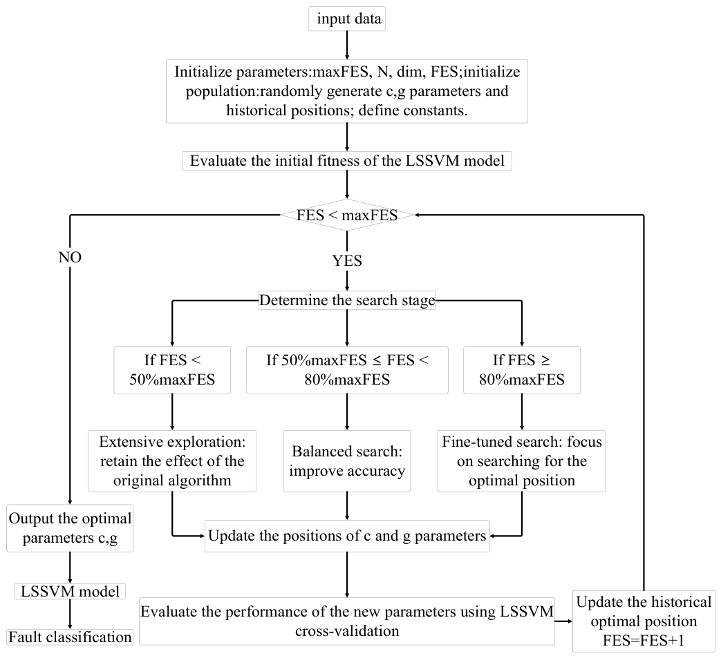Additionally, the ranges for the kernel function parameter $g$ and penalty factor $C$ are specified between 0.001 and 1000. Use seed 42. The EES iteratively explores the parameter space via its three evolutionary phases, with cross-validation accuracy serving as the fitness function. Following the optimization process, fault diagnosis is performed using LSSVM with the optimized parameter combination. The specific parameter optimization process is shown in Figure 1.

4. Transformer Fault Diagnosis with EES-LSSVM via Multidimensional Feature Fusion and SASYNO Sample Balancing

Transformers operating in outdoor natural environments over extended periods are susceptible to partial discharge or overheating faults caused by insulation aging and external intrusions. Such faults give rise to substantial changes in the composition and concentrations of dissolved gases within the insulating oil. Accordingly, the volume fractions of five key dissolved gases and their three-ratio coding are adopted as the characteristic parameters for fault diagnosis. The three-ratio coding is derived from the volumetric ratios of methane to hydrogen, acetylene to methane, and ethylene to ethane. These characteristic parameters can effectively indicate the operating condition of the equipment and therefore serve as critical foundations for transformer fault diagnosis.

4.1. Feature Selection

In dissolved gas analysis-based fault diagnosis of power transformers, the choice of feature set fundamentally governs the discriminative performance of the ensuing identification models. The five characteristic gases comprising hydrogen, methane, acetylene, ethylene, and ethane are routinely measured via chromatographic techniques and serve as the primary data source. Nevertheless, relying exclusively on the raw concentrations of these five gases for fault recognition suffers from inherent drawbacks. Variations in transformer oil volume, equipment service age, load current fluctuations, and fault energy release intensity all exert marked influences on the absolute generation rates of individual gas species. A given discharge fault may manifest as a moderate acetylene concentration in a large-capacity transformer but produce an exceedingly high acetylene peak in a small unit, and this concentration uncertainty severely compromises diagnostic consistency based on absolute values.

The incorporation of the three-ratio method transforms the raw concentration data into three dimensionless features, namely the ratios of methane to hydrogen, acetylene to ethylene, and ethylene to ethane. The primary advantage of this transformation lies in the effective cancellation of volumetric dilution effects arising from oil volume and sampling variations, because the paired gases possess comparable solubility and diffusivity properties such that the resulting ratios depend solely on the relative gas proportions generated by the fault rather than on equipment dimensions. More importantly, the three-ratio method is explicitly recommended by international standards including IEC 60599, and the coding intervals of these ratios have been rigorously validated through extensive field experience, thereby rendering the diagnostic conclusions both authoritative and traceable.

Consequently, the three-ratio method is incorporated as a supplementary feature vector in combination with the five characteristic dissolved gas concentrations to enhance the fault diagnosis of power transformers.

4.2. Data Sources and Classifications

The on-site monitoring data utilized in this study were acquired from a state grid substation in China and encompassed 952 fault records of power transformers. For each record, the feature set includes the dissolved gas concentrations of H₂, CH₄, C₂H₆, C₂H₄, and C₂H₂. During the data preprocessing stage, in addition to normal-state samples, we classified transformer bushing fault samples mainly into two major categories: discharge-related faults and overheating-related faults. The fault type labels follow the IEC 60599 standard, and the operational states of transformers are specifically categorized into the following seven classes: partial discharge, low-energy discharge, high-energy discharge, low-temperature overheating, medium-temperature overheating, high-temperature overheating, and normal state. For ease of model recognition and processing, these seven states are encoded as integer values from 1 to 7 in the order listed above. Prior to any oversampling operation, we partitioned the dataset into independent training and test sets via stratified sampling to ensure consistent class proportions in both subsets, with the training set comprising 761 samples and the test set containing 191 samples. In addition, a five-fold stratified cross-validation was conducted on the training set for model robustness evaluation. The distribution of sample counts for different fault types in the dataset is shown in

Table 1. Distribution of the number of samples by fault type.

Fault Type	Fault Coding	Total Samples	Actual Value	Test Value
Partial Discharge	1	130	104	26
Low-Energy Discharge	2	112	89	23
High-Energy Discharge	3	150	120	30
Thermal Fault (T < 300 °C)	4	80	64	16
Thermal Fault (300–700 °C)	5	125	100	25
Thermal Fault (T > 700 °C)	6	155	124	31
Normal	7	200	160	40

.

4.3. Data Preprocessing

In transformer fault diagnosis, the input features consist of eight variables: the concentrations of hydrogen, methane, ethane, ethylene, and acetylene dissolved in oil, together with three ratio features, namely CH₄/H₂, C₂H₂/C₂H₄, and C₂H₄/C₂H₆. The corresponding fault type labels are categorized into seven classes, including partial discharge, low-energy discharge, high-energy discharge, low-temperature overheating, medium-temperature overheating, high-temperature overheating, and normal condition. To remove the scale discrepancies among different features and thus improve the diagnostic accuracy, a column-wise min-max normalization is performed on the feature matrix. Let the feature matrix be $X=\left\{x_{i,j}\right\}$, where $i=1, 2,\dots ,N$ denotes the sample index, with $N$ being the total number of samples, and $j=1, 2,\dots , 8$ denotes the feature dimension index, corresponding to the eight input features including dissolved gases, CH₄/H₂, C₂H₂/C₂H₄, and C₂H₄/C₂H₆. The normalization is performed independently for each feature dimension using the following formula:

$${\tilde{X}}_{i,j}={\displaystyle \frac{X_{i,j} - {\min }_{k\in D_{train}}{X}_{k,j}}{{\max }_{k\in D_{train}}{X}_{k,j} - {\min }_{k\in D_{train}}{X}_{k,j}}}$$

(23)

where $D_{train}$ denotes the training set; ${min}_{k\in D_{train}}{x}_{k,j}$ and ${max}_{k\in D_{train}}{x}_{k,j}$ are the minimum and maximum values of the j-th feature computed exclusively from the training data. After this column-wise normalization, the value of each feature across all samples is scaled to the interval $[0, 1]$, while the distinct physical units and scales of different features are preserved.

4.4. Handling of Original Sample Imbalance Based on SASYNO

The transformer fault samples are characterized by a highly imbalanced distribution. Specifically, 160 samples are associated with the normal state, while only 64 samples are associated with the thermal fault state. Due to this imbalanced distribution, the diagnostic model is easily biased toward the majority class, and consequently, the fault category is misclassified as normal, which may trigger serious operational risks. To improve the diagnostic accuracy on minority class faults, an oversampling data generation method is introduced for balancing the imbalanced sample set.

After oversampling was applied by the SASYNO method, the increments for partial discharge, low-energy discharge, high-energy discharge, low-temperature overheating, medium-temperature overheating, and high-temperature overheating were 56, 71, 40, 96, 60, and 36, respectively. The total sample size increased from 761 to 1120, and the imbalance problem of the original data distribution was effectively alleviated. The detailed distribution of minority class samples before and after data processing is shown in

Table 2. Sample distribution after SASYNO imbalance processing.

	Sample Distribution of Different Fault Types
Data type	1	2	3	4	5	6	7
Original data	104	89	120	64	100	124	160
SASYNO-processed data	160	160	160	160	160	160	160

.

4.5. Fault Diagnosis Process

The dissolved gases in transformer oil, together with the three ratios CH₄/H₂, C₂H₂/C₂H₄, and C₂H₄/C₂H_6, are selected as key features for fault identification, and the EES-LSSVM method is adopted for diagnosis. Although a high recognition accuracy is achieved by this method, the consistency of diagnostic results is poor due to the imbalance of the original data samples. To address this issue, the SASYNO method is introduced to balance the data, by which the balance of data distribution and the expansion of samples can be effectively achieved while the original data characteristics are maintained. Finally, transformer fault diagnosis is conducted again using the balanced dataset after processing:

(1)

In the algorithm initialization stage, parameter configuration is first completed, including setting parameters such as the maximum number of evaluations, population size, and dimensionality. Subsequently, an initial population is randomly generated and evaluated by calculating the initial fitness. Furthermore, the performance of the current solution is verified using the LSSVM model, and the corresponding optimal parameter combination is output.

(2)

The algorithm dynamically adjusts the search strategy according to the evaluation progress: when the number of evaluations is less than 50% of the maximum value, global exploration is performed to maintain population diversity; when the number of evaluations is between 50% and 80%, the algorithm shifts to a balanced search that balances exploration and exploitation to enhance solution quality; if the number of evaluations exceeds 80% (which can be adjusted to, for example, 85% or 90% according to the actual situation), the algorithm enters a local intensive exploitation phase to strengthen local search capability and improve solution accuracy.

(3)

In each iteration, the algorithm first updates the parameter positions according to the corresponding strategy. Subsequently, LSSVM cross-validation is employed to evaluate the performance of the new parameters, and the historical optimal solution is updated accordingly. After that, the number of evaluations is incremented, and the cycle repeats until the termination condition is satisfied. Finally, the obtained global optimal parameters are substituted into the LSSVM model for fault diagnosis.

5. Simulation Verification and Comparative Analysis

The simulation experiments in this paper were conducted on a computer equipped with 16 GB RAM, a 12th Gen Intel(R) Core(TM) i7-12700H processor, and a 64-bit Windows operating system, and Matlab 2024B was used as the simulation software.

5.1. Comparative Analysis

(1)

Fault Diagnosis Comparison Under Imbalanced Sample Handling

As shown in Table 1, the data distribution of each fault type exhibits significant differences, with low-temperature overheating samples accounting for only 8.4% of the total while normal samples account for as much as 21%. This severely imbalanced data distribution greatly restricts the consistency performance of the transformer fault diagnosis model.

To this end, the training set was processed by the SASYNO method, through which the minority class samples were effectively expanded and the data scales of all classes were balanced to the same order of magnitude.

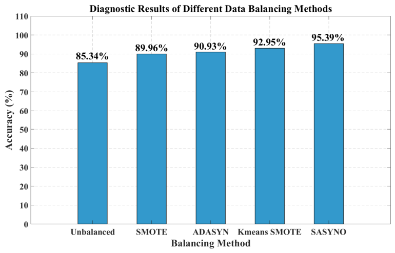
To systematically evaluate the effectiveness of the data balancing method adopted in this study, the original dataset, along with the balanced datasets processed by four algorithms—SASYNO, Synthetic minority oversampling technique (SMOTE), adaptive synthetic sampling (ADASYN), and K-means Synthetic minority oversampling technique (IK-means SMOTE)—are selected and input into the EES-LSSVM transformer fault diagnosis model, and their respective evaluation metrics are recorded. The final diagnostic results are summarized in Figure 2.

Based on the data in the figure above, the model achieves the least satisfactory diagnostic performance when using the original imbalanced data, with an accuracy of only 85.34%. After applying various data balancing methods, all evaluation metrics of the model are improved. Among them, the SASYNO algorithm adopted in this study performs the best, increasing the accuracy to 95.39%, which is superior to the other methods.

(2)

Accuracy Comparison Among Different Models

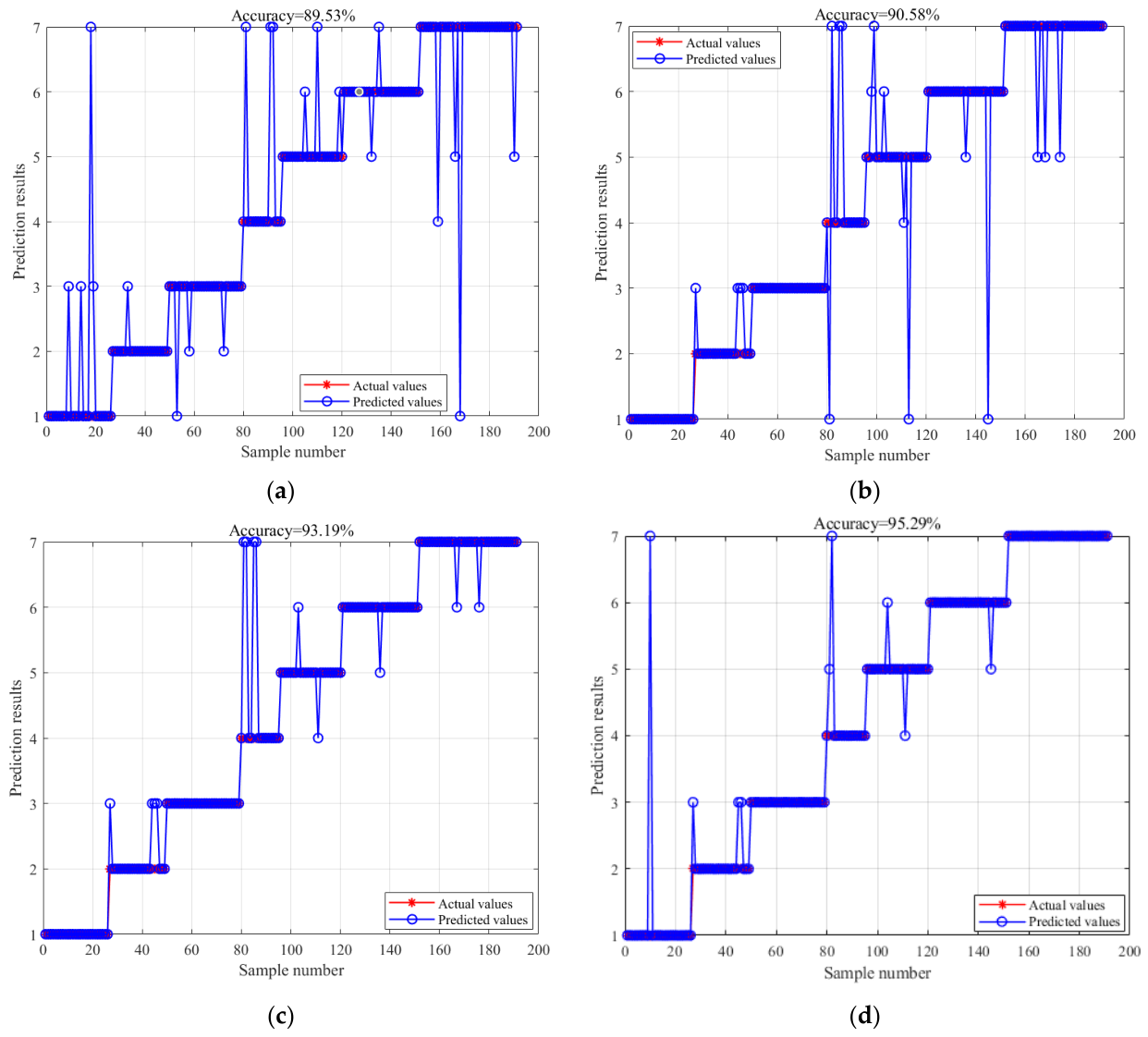
To evaluate the fault diagnosis accuracy of the proposed method in this study, experiments are conducted using a dataset composed of selected optimal features as input. Four models—Back Propagation Neural Network (BP neural network), LSSVM, Tuna Swarm Optimization-based LSSVM (TSO-LSSVM), and Experience Exchange Strategy-based LSSVM (EES-LSSVM)—are respectively employed for transformer fault diagnosis. The diagnostic accuracy serves as the core evaluation metric for model performance, and the fault diagnosis results of each method are compared, as shown in Figure 3.

The EES-LSSVM model achieved the highest test accuracy of 95.29%, substantially outperforming the BP neural network, the standard LSSVM, and the TSO-LSSVM, which yielded test accuracies of 89.53%, 90.58%, and 93.19%, respectively. In comparison with these three reference models, the improvements in fault diagnosis accuracy obtained by EES-LSSVM were 5.76, 4.71, and 2.1 percentage points, respectively. As shown in

Table 3. Comparison of Diagnostic Results Using Different Feature Types and Methods.

	BP Neural Network	LSSVM	TSO-LSSVM	EES-LSSVM
With three-ratio features	89.53%	90.58%	93.19%	95.29%
Dissolved gas only	87.96%	89.01%	92.14%	93.72%

, the introduction of three-ratio features slightly improves the accuracy.

Five repeated experiments were conducted with five-fold cross-validation to evaluate the BP neural network, the LSSVM, the TSO-LSSVM, and the EES-LSSVM. The diagnostic accuracies were 89.32% ± 1.35%, 90.36% ± 1.54%, 93.29% ± 0.70%, and 95.39% ± 0.39%, respectively. The EES-LSSVM achieved the highest accuracy and the smallest standard deviation, which confirms the effectiveness of the EES in enhancing diagnostic performance and stability.

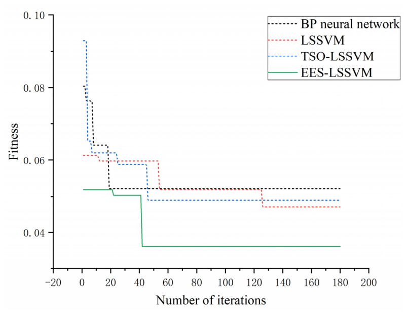
To further investigate whether optimizing the network parameters of LSSVM using EES helps improve the performance of transformer fault diagnosis, the fitness curves of four models—BP neural network, LSSVM, TSO-LSSVM, and EES-LSSVM—after 180 iterations are compared, as shown in Figure 4. The BP neural network converges to a fitness value of 0.0522 at the 22nd iteration, while LSSVM converges to 0.0472 at the 126th iteration. Although TSO-LSSVM converges to 0.0490 at the 46th iteration, EES-LSSVM converges to 0.0361 at the 42nd iteration, demonstrating the rapid convergence and effectiveness of the EES optimization. Furthermore, compared with TSO-LSSVM, EES-LSSVM achieves a smaller fitness value of 0.0361, verifying the superiority of the proposed method in terms of optimization accuracy.

5.2. Fault Diagnosis Model Evaluation

To systematically evaluate the comprehensive performance of the proposed diagnostic method, this paper introduces accuracy (${\mathsf{\eta }}_{\mathrm{accuracy}}$) and recall (${\mathsf{\eta }}_{\mathrm{recall}}$) as evaluation metrics. Their specific mathematical definitions are as follows:

$${\eta }_{accuracy}={\displaystyle \frac{n}{N}}$$

(24)

$${\eta }_{recall}={\displaystyle \frac{n_T}{n_R}}$$

(25)

In the formula, $n$ is the total number of correctly diagnosed samples, and $N$ is the total number of all samples. For a specific fault category under evaluation, $n_T$ denotes the number of samples correctly identified by the model, and $n_R$ represents the actual total number of samples belonging to that fault category.

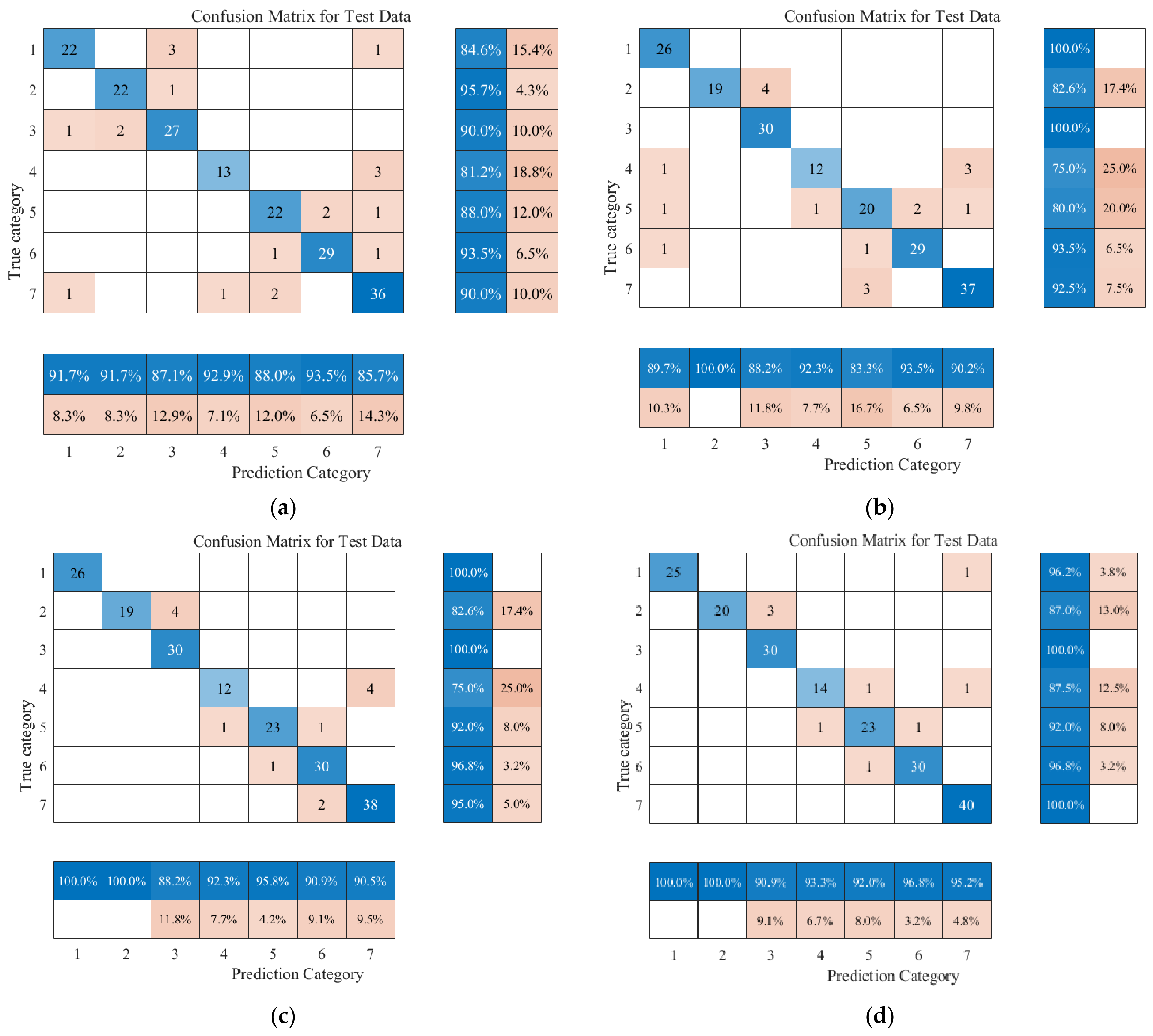
Figure 5 presents the confusion matrix of transformer fault diagnosis obtained using the proposed method, and the corresponding evaluation metrics are listed in

Table 4. Results of confusion matrix for each model.

Type	Precision/%							Recall/%
	1	2	3	4	5	6	7	1	2	3	4	5	6	7
BP neural network	84.6	95.7	90.0	81.2	88.0	93.5	90.0	91.7	91.7	87.1	92.9	88.0	93.5	85.7
LSSVM	100	82.6	100	75.0	80.0	93.5	92.5	89.7	100	88.2	92.3	83.3	93.5	90.2
TSO-LSSVM	100	82.6	100	75.0	92.0	96.8	95.0	100	100	88.2	92.3	95.8	90.9	90.5
EES-LSSVM	96.2	87.0	100	87.5	92.0	96.8	100	100	100	90.9	93.3	92.0	96.8	95.2

. In this confusion matrix, the sum of elements in any column represents the total number of actual samples belonging to that fault category; the sum of elements in any row represents the total number of samples predicted as that fault category; and the sum of the diagonal elements represents the total number of samples correctly classified across all fault categories.

A comparative analysis of the confusion matrices for the four models reveals that the EES-LSSVM achieves the highest overall classification accuracy. As presented in Table 4, the EES-LSSVM yields recall rates exceeding 90% for all seven fault categories, with perfect recall for categories 1 and 2, and precision values above 90% for five categories, although categories 2 and 4 show a precision of 87.0 and 87.5%. In contrast, the back-propagation neural network exhibits markedly lower precision for category 4 at 81.2% and for category 5 at 88.0%. The standard LSSVM and the TSO-LSSVM both suffer from inferior performance on categories 2, 4, and 5, with precision values of 82.6%, 75.0%, and 80.0% respectively for these two models. The EES-LSSVM substantially improves the identification accuracy for these challenging categories, attaining 87.0% for category 2, 87.5% for category 4, and 92.0% for category 5. Compared with the TSO-LSSVM, the EES-LSSVM not only increases precision across all categories but also maintains higher and more stable recall rates, particularly for categories 1, 3, and 7. Overall, owing to its more effective evolutionary optimization strategy, the EES-LSSVM not only achieves superior classification accuracy but also effectively reconciles the trade-off between missed detections and false alarms across different fault types, thereby enabling more thorough extraction of fault signatures and significantly reducing inter-class confusion.

6. Discussion

Addressing the issue of power transformer fault diagnosis, this study constructs a diagnostic model that integrates multi-dimensional features with intelligent algorithms. On the basis of traditional dissolved gas analysis, the three-ratio method is introduced to supplement the feature vector. Meanwhile, the SASYNO method is employed to balance minority-class samples, and EES is utilized to optimize LSSVM parameters, ultimately achieving a diagnostic accuracy of 95.29%.

At the feature level, this study combines the volume fractions of five dissolved gases with three-ratio coding to form an eight-dimensional input vector. Traditional DGA methods typically rely solely on gas concentrations or single ratios, which inadequately capture the complex evolution patterns of dissolved gases under fault conditions. The introduction of three-ratio coding effectively eliminates the influence of oil volume variations, sampling errors, and equipment capacity differences on absolute concentration values, thereby rendering the feature representation more robust and interpretable. Experimental data indicate that incorporating three-ratio features consistently improves diagnostic accuracy across all models, with the EES-LSSVM model achieving an increment of approximately one percentage point. Although this increment appears modest, it carries practical engineering significance in multi-class tasks, particularly for ambiguous categories such as medium-temperature overheating and low-energy discharge, where ratio features markedly reduce misclassification rates.

During the experiments, the SASYNO method, by accurately identifying neighboring samples and applying Gaussian perturbations, embeds synthetic samples within the minority class decision region and exhibits notable resistance to overlap. Regarding the legitimate concern that the high-energy discharge category might suffer from overfitting after being expanded from 64 to 160 samples, the algorithmic design of SASYNO offers quantitative guarantees from three aspects: candidate selection employs a data-adaptive threshold, perturbation magnitude is calibrated by per-dimension standard deviation, and the final linear interpolation constraint collectively ensures that synthetic samples remain separable from the majority class [15]. The LSSVM classifier further provides regularization through its structural risk minimization principle and support-vector-determined decision boundary, while the EES-optimized parameters adjust the bias-variance trade-off. The original SASYNO study confirms that overfitting occurs only when the training set becomes extremely large; under the sample conditions characterizing our dataset, this method consistently improves performance without introducing spurious patterns, thus offering clear advantages over traditional oversampling approaches. The five-fold cross-validation results, with a standard deviation of only 0.39% for the EES-LSSVM model employing SASYNO sample balancing compared with 1.35% for the BP neural network, experimentally corroborate the stability and generalization capacity of the proposed model.

The SASYNO algorithm resists overlap through three complementary mechanisms: data-adaptive neighborhood screening confines synthetic samples to authentic local regions of the minority class, per-dimension Gaussian perturbation prevents excessive deviation from the data manifold, and linear interpolation avoids intrusion into majority class regions. Future work will incorporate direct overlap metrics and feature space visualization for more comprehensive quantitative evaluation.

Several limitations of this study should be acknowledged. First, the data originate from a single regional substation and may not encompass the full diversity of fault patterns under varying climatic conditions, voltage levels, and service ages; the cross-domain generalizability of the model requires further validation. Second, although three-ratio coding is incorporated, other established ratio systems such as the Duval triangle and Rogers ratios have not been included, nor have dynamic features like gas generation rates been considered. Third, the computational complexity of the EES algorithm increases with population size and iteration count, potentially posing an efficiency bottleneck in real-time online diagnosis scenarios. Fourth, the current statistical analysis relies on cross-validation means and standard deviations without incorporating more elaborate significance tests. In response to these limitations, future work will focus on expanding and validating cross-regional datasets, exploring more diversified feature combination schemes, investigating lightweight or distributed optimization strategies to enhance algorithmic responsiveness, and systematically incorporating confidence interval estimation and formal hypothesis testing to provide a more robust statistical foundation for the proposed diagnostic framework.

7. Conclusions

To tackle the problem of transformer fault diagnosis and classification, this study proposes a diagnostic method based on EES-LSSVM, which integrates multidimensional feature fusion and adopts the SASYNO sample balancing technique. The principal conclusions are summarized as follows:

(1)

To enhance the diagnostic accuracy of transformer fault identification, three-ratio features, namely CH₄/H₂, C₂H₂/C₂H₄, and C₂H₄/C₂H₆, are introduced in addition to the five dissolved gas concentrations. The integration of these comprehensive features markedly improves fault recognition performance compared with schemes relying solely on the five gas concentrations, thereby validating the feasibility and superiority of the proposed feature augmentation approach.

(2)

The SASYNO method generates synthetic samples through neighborhood sample screening, Gaussian perturbation, and linear interpolation. This process effectively expands the decision regions of minority classes while avoiding overlap with majority class samples, thus substantially alleviating the classification bias induced by data imbalance.

(3)

In comparison with the back-propagation neural network, the standard LSSVM, and the TSO-LSSVM, the proposed EES-LSSVM achieves accuracy improvements of 5.76, 4.71, and 2.1 percentage points, respectively. These results demonstrate the marked advantage of the experience exchange strategy in parameter optimization and provide robust support for practical engineering applications.