Unseen-Cell SOH Prediction via Energy-Aware Warm-Up and Degradation-Consistency Constraints

Abstract

State of health (SOH) is a key indicator for safety monitoring, lifetime assessment, and maintenance decisions in lithium-ion battery management systems. However, differences in initial capacity, degradation rate, local capacity variation, and health-indicator evolution often cause models trained on limited source cells to produce biased predictions and unstable trajectories on unseen cells. To address this challenge, we develop the Energy-Aware Warm-Up with Degradation-Consistency Constraints (EWDC) framework for unseen-cell SOH prediction. EWDC couples partial-charge health-indicator extraction, health-indicator graph encoding, cycle-to-cycle degradation-increment prediction, and recursive SOH-trajectory reconstruction. Within-dataset leave-one-battery-out validation was conducted separately on the NASA and CALCE-CS2 datasets. Across the eight held-out cells, EWDC achieved average RMSE, MAE, and $R^2$ values of 1.21%, 0.65%, and 0.975, respectively. Relative to the GNN baseline, EWDC reduced average RMSE and MAE by 32.19% and 38.83%, respectively. Additional limited-source-battery experiments and ablation studies suggest that EWDC improves within-dataset unseen-cell prediction accuracy.

1. Introduction

Lithium-ion batteries are widely deployed in electric vehicles, energy storage systems, and portable devices, while progressive aging reduces their usable capacity and operational reliability. State of health (SOH), defined by the retained capacity relative to the initial state, is therefore a core indicator for safety monitoring, lifetime assessment, and maintenance scheduling in battery management systems [1,2,3,4,5,6,7]. In practical SOH estimation, the challenge is not only to fit the degradation trajectories of known cells but also to generate reliable SOH trajectories for previously unseen cells whose degradation rates, local fluctuations, and indicator evolution patterns differ from the limited source cells available for training [8].

Among data-driven SOH approaches, partial-charge information is especially attractive because complete charge–discharge records are often unavailable in online operation. Prior studies have shown that short charging segments can support state estimation or degradation-feature extraction from voltage, current, and time measurements [9,10,11,12]. However, these partial-charge observations are still commonly organized as conventional vectors or temporal sequences, so the dependencies among health indicators (HIs) remain only implicitly represented. As a result, such representations may preserve individual feature trends but fail to adequately capture how multiple HIs jointly reflect the same degradation state.

Graph-based SOH methods address part of this limitation by modeling HIs as relational objects rather than isolated features. Yao et al. demonstrated the value of graph-structured HI representation for SOH estimation, and Gu et al. further explored dynamically adapted HI relationships during degradation [13,14]. These studies strengthen relational representation, but most graph-based formulations still treat absolute SOH as the primary output. For unseen-cell prediction, an additional issue is how cycle-to-cycle degradation variation accumulates into a full SOH trajectory. This motivates a formulation that not only encodes HI dependencies, but also predicts signed degradation increments and reconstructs SOH recursively over successive cycles.

Generalization across cells introduces a second difficulty. Existing transfer-learning and adaptation studies have improved battery-state prediction by transferring knowledge across batteries or operating domains [15,16,17,18]. Yet these approaches commonly rely on target-domain adaptation, target-domain exposure, or target-specific fine-tuning. By contrast, the present study focuses on a stricter source-only within-dataset leave-one-battery-out (LOBO) setting, in which the held-out target cell contributes no SOH labels and receives no target-specific adaptation during training. Under this protocol, the model must learn both feature relationships and degradation evolution solely from the limited source cells.

A third issue concerns optimization under limited-source conditions. Adding noise to training inputs can regularize learning and enlarge local neighborhoods [19], but uniform input perturbation does not distinguish samples according to their relative positions in the source distribution. Samples near the distribution center and samples near the boundary may therefore receive similarly scaled perturbations even though their roles in source-only generalization differ. This limitation motivates a distribution-aware staged perturbation strategy that adapts the perturbation magnitude to each sample’s source-distribution position and gradually relaxes it during training.

A fourth issue concerns trajectory plausibility. Physics-guided and prior-guided learning has improved the stability of battery degradation prediction by incorporating physical knowledge, degradation constraints, or structured regularization [20,21,22,23]. Nevertheless, when SOH is generated recursively from predicted cycle-level changes, constraining only the reconstructed SOH states is insufficient to regulate the intermediate degradation increments that produce those states. Conversely, constraining only local increments cannot fully control the plausibility of the reconstructed trajectory. For this reason, recursive SOH generation calls for coordinated constraints on both the generated SOH states and the degradation increments. In the present work, these constraints are formulated as soft empirical degradation priors rather than mechanistic electrochemical equations.

These research directions are complementary but are typically formulated separately.

Table 1. Methodological positioning of EWDC relative to representative prior studies.

Research Line	Representative Studies	Established Formulation	Formulation in EWDC
Partial-charge representation	Tian et al. [12]; Yang et al. [10]	Short charging segments for state estimation or degradation-feature extraction	CC–CV partial-charge HIs used as graph-node information
HI relational modeling	Yao et al. [13]; Gu et al. [14]	Graph-based or dynamically adapted HI relationships for SOH estimation	Learnable HI graph with GCN-based dependency encoding
Cross-cell adaptation	Kim et al. [15]; Huang et al. [18]	Transfer learning or target-domain adaptation across batteries/domains	Source-only within-dataset LOBO without target-cell fine-tuning
Degradation change modeling	Yang et al. [24]	Cycle-wise degradation changes used as complementary health information	Signed $\Delta$SOH used as the direct target for recursive SOH reconstruction
Prior-guided regularization	Bishop [19]; Wang et al. [23]	Noise regularization or physics-informed degradation constraints	Distribution-aware staged perturbation and two-level degradation-consistency constraints

summarizes their relationship to the present study.

The comparison highlights a coupled research gap: HI dependency representation, cycle-to-cycle degradation evolution, limited-source optimization, and trajectory plausibility are often improved in isolation, even though they govern successive parts of the same prediction process. For within-dataset unseen-cell SOH prediction, these factors must instead be handled jointly. The representation used for partial-charge HIs influences how degradation dependencies are learned; the prediction target determines whether local cycle-to-cycle change is explicitly modeled; the source-only training strategy affects how strongly the model overfits limited source patterns; and the constraint design determines whether the generated trajectory remains plausible throughout recursion.

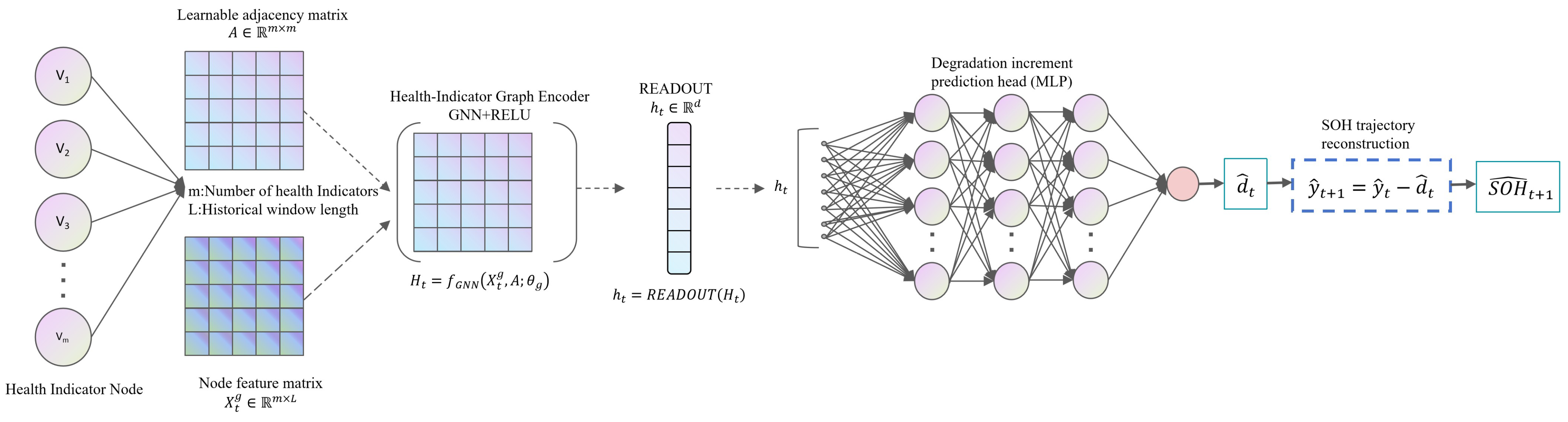
To address this coupled problem, we develop the Energy-Aware Warm-Up with Degradation-Consistency Constraints (EWDC) framework. EWDC links a learnable HI graph, signed $\Delta$SOH prediction, recursive SOH reconstruction, an energy-aware three-stage warm-up strategy, and two-level degradation-consistency constraints into one coordinated trajectory-generation framework. These components are not treated as independent add-on modules: graph encoding provides the relational representation used for increment prediction, signed degradation increments define the recursive transition between adjacent SOH states, staged perturbation regularizes the source-only optimization of that transition, and the two-level constraints act jointly on the generated states and increments of the same recursive process.

Accordingly, EWDC integrates HI relational modeling, degradation-increment prediction, staged perturbation, and empirical degradation priors into a unified trajectory-oriented framework for source-only unseen-cell prediction. Experiments are conducted separately on the NASA and CALCE-CS2 datasets under within-dataset LOBO evaluation. Across the eight held-out cells, EWDC achieved an average RMSE of 1.21%, an average MAE of 0.65%, and an average $R^2$ of 0.975, while reducing RMSE and MAE by 32.19% and 38.83%, respectively, relative to the GNN baseline.

The main contributions are threefold:

1.

We formulate a trajectory-oriented graph prediction framework that couples learnable HI dependency encoding, signed cycle-to-cycle $\Delta$SOH prediction, and recursive SOH reconstruction.

2.

We introduce a source-distribution-aware three-stage warm-up strategy for limited-source, source-only training, without using target-cell SOH labels or target-specific fine-tuning.

3.

We impose two-level degradation-consistency constraints that jointly regulate reconstructed SOH states and degradation increments during recursive trajectory generation.

The remainder of this paper is organized as follows. Section 2 presents the datasets, health-indicator construction, the within-dataset unseen-cell prediction task, and the EWDC formulation. Section 3 reports the experimental setup, LOBO results, limited-source evaluation, ablation studies, and sensitivity analyses. Section 4 concludes the paper by discussing the main findings, limitations, and future work.

2. Data and Methods

2.1. Datasets and Health-Indicator Construction

Experimental data were taken from the NASA lithium-ion battery aging dataset [25] and the CALCE battery dataset [26]. We selected batteries B0005, B0006, B0007, and B0018 from the NASA dataset, together with CS2-35–CS2-38 from the CALCE-CS2 dataset, for evaluation. Both datasets record capacity evolution during battery cycling together with the corresponding charging measurements. The capacity degradation curves are shown in Figure 1.

As summarized in

Table 2. Dataset provenance and experimental conditions of the selected batteries.

Item	NASA	CALCE-CS2
Selected cells	B0005, B0006, B0007, B0018	CS2-35, CS2-36, CS2-37, CS2-38
Cell type/chemistry	18650 Li-ion	LiCoO2 prismatic Li-ion
Nominal capacity	2.0 Ah	1.1 Ah
Charging protocol	CC 1.5 A to 4.2 V, followed by CV to 20 mA	CC 0.5 C to 4.2 V, followed by CV to 0.05 A
Discharge current	2.0 A	1C
Discharge cut-off voltage	B0005: 2.7 V; B0006: 2.5 V; B0007: 2.2 V; B0018: 2.5 V	2.7 V
Temperature	24 °C	Room temperature

, the NASA and CALCE-CS2 cells differ in nominal capacity, cell configuration, chemistry, charging/discharging conditions, and cutoff settings. Therefore, the two datasets are treated as separate experimental domains rather than as a pooled homogeneous dataset.

Both datasets employ CC-CV charging, enabling the same partial-charge health-indicator extraction framework to be applied under their respective operating conditions.

Battery health is expressed by the capacity-retention ratio

$$y_i={\mathrm{SOH}}_i={\displaystyle \frac{Q_i}{Q_0}}.$$

(1)

Here, $Q_i$ is the measured discharge capacity at cycle i, and $Q_0$ is the measured discharge capacity of the initial reference cycle of the same cell. The SOH labels used for model training and performance evaluation are calculated directly from the measured capacities without smoothing or interpolation. Thus, the initial reference cycle satisfies $y_1=1$ by definition. The lightly smoothed SOH sequence introduced later is used only to construct the local trend-consistency term and does not replace the original SOH labels. No target-specific denoising or multi-cycle calibration is applied to $Q_0$; the measured capacity of the initial reference cycle is used consistently for SOH normalization.

We extract general health indicators from the voltage, current, and time sequences during cyclic charging. For all cells, the partial-charge segments are extracted using the same predefined rule. Within each charging cycle, the CC feature window consists of the chronologically ordered samples in the terminal-voltage interval of 4.0–4.2 V, while the CV feature window consists of the samples during the charging-current decay from 0.5 to 0.1 A. Health indicators are calculated only from measurements available within these completed segments, without using subsequent-cycle or future information. Cycles with incomplete partial-charge segments were excluded from feature construction. The extracted CC-CV segments are used to derive features such as duration, cumulative charged quantity, statistical moments, variation slopes, and curve entropy [10,11,12,27,28,29,30,31,32], while the cycle index is included to represent the battery degradation stage.

The selected HIs jointly characterize complementary aspects of degradation-related evolution during battery aging.

The required voltage, current, and time signals are routinely available from a BMS. The current implementation assumes that the specified CC-CV segments can be reliably identified and are sufficiently complete for feature calculation. No target-cell SOH or discharge-capacity information is required during inference. Nevertheless, substantial deviations from the evaluated charging-current or temperature conditions, severely incomplete charging segments, or significant measurement noise may affect feature reliability and require further adaptation. The health-indicator vector at the ith cycle is written as

$${\mathbf{x}}_i={\left[x_{i,1},x_{i,2},\dots ,x_{i,m}\right]}^{\mathrm{T}}\in {\mathbb{R}}^m,$$

(2)

where $m=17$ denotes the health-indicator dimension used in this study. All features are aligned according to cycle order. In each within-dataset LOBO run of this study, the standardization parameters are estimated only from the training data of the source cells and then applied uniformly to the validation and target cells, thereby preventing information leakage from the held-out target cell during model training.

2.2. Prediction Task and Overall Framework

For an arbitrary battery b, its cycle data are represented as

$${\mathcal{D}}^{\left(b\right)}={\left\{\left({\mathbf{x}}_i^{\left(b\right)},y_i^{\left(b\right)}\right)\right\}}_{i=1}^{N_b},$$

(3)

where ${\mathbf{x}}_i^{\left(b\right)}$ denotes the extracted and standardized health-indicator vector of battery b at the ith cycle, $y_i^{\left(b\right)}$ is the corresponding ground-truth SOH, and $N_b$ is the number of valid cycles of that battery.

Let the source-battery set and target-battery set be ${\mathcal{B}}_s$ and ${\mathcal{B}}_t$, respectively. Their corresponding datasets are

$${\mathcal{D}}_s=\bigcup _{b\in {\mathcal{B}}_s}{\mathcal{D}}^{\left(b\right)},{\mathcal{D}}_t=\bigcup _{b\in {\mathcal{B}}_t}{\mathcal{D}}^{\left(b\right)},{\mathcal{B}}_s\cap {\mathcal{B}}_t=⌀.$$

(4)

Model training and validation are both performed on the source-battery data ${\mathcal{D}}_s$. During testing, the target battery provides only the health-indicator sequence; its ground-truth SOH does not participate in parameter updating or model selection and is used only for final performance evaluation. Therefore, the objective of unseen-cell SOH prediction is to use degradation information from the source batteries to generate the SOH trajectory of a target battery that is not involved in training.

In the experiments of this study, ${\mathcal{B}}_s$ and ${\mathcal{B}}_t$ are drawn from the same dataset in each LOBO fold. NASA and CALCE-CS2 are evaluated independently and are not mixed during training or testing. Therefore, the experimental protocol evaluates within-dataset unseen-cell generalization and does not constitute cross-dataset transfer between NASA and CALCE-CS2.

Because batteries differ in degradation rate, local capacity variation, and health-indicator evolution patterns, directly learning a mapping from health indicators to absolute SOH may lead to biased target-battery predictions when source-specific local relationships do not generalize. The overall mapping of EWDC is defined as

$$\widehat{y}=F_{\mathrm{EWDC}}(X;\mathsf{\Theta })=\mathcal{R}\left[f_{\Delta }\left(f_g(X;{\theta }_g);{\theta }_{\Delta }\right)\right],$$

(5)

with the trainable parameter set

$$\mathsf{\Theta }=\left\{{\theta }_g,{\theta }_{\Delta }\right\}.$$

(6)

Here, X denotes the historical health-indicator sequence, $f_g(·)$ is the health-indicator graph encoder, $f_{\Delta }(·)$ is the degradation-increment prediction head, and $\mathcal{R}(·)$ is the recursive SOH reconstruction process. EWDC first extracts degradation representations from the historical health indicators, then predicts the degradation increment between adjacent cycles, and finally reconstructs the complete SOH trajectory recursively. The energy-aware warm-up acts on the training inputs, whereas the degradation-consistency constraints act on the joint optimization objective.

2.3. Trajectory Modeling via Degradation Increments

Conventional SOH prediction models usually establish a direct mapping between current-cycle health indicators and SOH [9,24,32]

$${\widehat{y}}_t=f(X_t;\theta ),$$

(7)

where $X_t$ denotes the health-indicator input at the tth cycle and $\theta$ denotes the model parameters. This formulation treats different cycles as relatively independent samples and does not explicitly connect adjacent-cycle degradation variation with the complete SOH trajectory.

To overcome this limitation, we reformulate the prediction target by replacing absolute SOH with the signed degradation increment between adjacent cycles

$$d_t=y_t-y_{t+1},t=1,2,\dots ,T-1.$$

(8)

Accordingly, $d_t>0$ indicates SOH degradation, whereas $d_t<0$ represents a local SOH recovery. The model predicts the SOH change from cycle t to cycle $t+1$ and then reconstructs the full SOH trajectory recursively from the sequence of predicted degradation increments.

For the tth prediction position, a historical health-indicator window of length L is constructed as

$$X_t={\left[{\mathbf{x}}_{t-L+1},{\mathbf{x}}_{t-L+2},\dots ,{\mathbf{x}}_t\right]}^{\mathrm{T}}\in {\mathbb{R}}^{L\times m},$$

(9)

where m is the health-indicator dimension, ${\mathbf{x}}_t$ is the extracted and standardized multi-source health-indicator vector at the tth cycle, and L is the historical window length. This window preserves the recent evolution of the health indicators and provides continuous input for degradation-representation extraction.

Different health indicators are not mutually independent. For example, voltage variation, constant-voltage charging-current decay, and charging duration may jointly reflect internal polarization and capacity degradation. To characterize these latent relationships, the health indicators are organized as a graph structure [13,33]

$${\mathcal{G}}_t=\left({\mathcal{V}}_t,{\mathcal{E}}_t,X_t^g,A\right),X_t^g=X_t^{\mathrm{T}}\in {\mathbb{R}}^{m\times L},A\in {\mathbb{R}}^{m\times m},$$

(10)

where ${\mathcal{V}}_t$ is the node set, ${\mathcal{E}}_t$ is the edge set, $X_t^g$ is the node-feature matrix, and A is a learnable adjacency matrix. Each node corresponds to one health indicator. The node features are formed by the variation sequence of the corresponding health indicator within the historical window, while the learnable adjacency matrix provides trainable edge weights for information propagation among HIs. These edge weights are jointly optimized with the graph encoder and degradation-increment predictor during source-battery training.

The HI graph adopts a fully connected candidate topology, and its learnable edge weights are optimized using source-battery data only within each LOBO fold. Self-loops are added to the adjacency matrix, followed by symmetric normalization $\widehat{A}=D^{-1/2}(A+I)D^{-1/2}$. A two-layer GCN with a hidden dimension of 64 is used for feature propagation, and mean pooling is applied to obtain the graph-level representation for degradation-increment prediction. No additional sparsity constraint is imposed on the adjacency weights.

The node-feature matrix and adjacency matrix are fed into the health-indicator graph encoder to obtain node embeddings that integrate information across health indicators

$$H_t=f_g\left(X_t^g,\widehat{A};{\theta }_g\right),$$

(11)

where ${\theta }_g$ denotes the trainable parameters of the graph encoder. Specifically, $f_g(·)$ consists of two graph convolutional layers with ReLU activation between them. Through graph information propagation, nonlinear activation, and feature transformation, the node embedding $H_t$ integrates the historical evolution of each health indicator and the information propagated from the other HIs.

Because SOH prediction is a graph-level regression task, the node embeddings of all health indicators must be aggregated into a unified degradation representation. We use mean pooling to obtain the graph-level representation corresponding to the current historical window

$$h_t=\mathrm{MeanPool}\left(H_t\right),h_t\in {\mathbb{R}}^{64},$$

(12)

where the pooled graph-level degradation representation remains 64-dimensional.

The degradation-increment prediction head then uses a multi-layer perceptron (MLP) to map the graph-level representation to the predicted degradation increment from cycle t to cycle $t+1$

$${\widehat{d}}_t=f_{\Delta }\left(h_t;{\theta }_{\Delta }\right).$$

(13)

Because the SOH of each battery is normalized by its initial capacity, the recursive process uses the SOH of the first valid cycle as the initial state

$${\widehat{y}}_1=1,{\widehat{y}}_{t+1}={\widehat{y}}_t-{\widehat{d}}_t,t=1,2,\dots ,T-1.$$

(14)

The same recursive strategy is used during training and inference. The initialization ${\widehat{y}}_1=1$ follows directly from the relative SOH definition and does not require access to target-cell ground-truth SOH during inference. In particular, the target cell does not require true SOH labels, measured discharge capacity, or an additional target-specific calibration step to initialize the recursive predictor. After initialization, all subsequent states are generated solely from the predicted degradation increments. Ground-truth SOH is used only for training-loss computation and offline final evaluation and is not fed into the next recursive step. Accordingly, target-cell discharge capacities are used only offline to construct the reference SOH trajectory for final evaluation, rather than to drive the recursive prediction process.

This modeling strategy serves two purposes. First, degradation increments focus directly on local changes between adjacent cycles and can reduce the influence of differences in absolute SOH levels and capacity scales among batteries. Second, the recursive relationship explicitly links local degradation increments to the full SOH trajectory, enabling the model to describe battery aging as a continuous degradation process rather than as isolated state points. Figure 2 summarizes the resulting prediction architecture, which combines health-indicator graph encoding with recursive degradation-increment prediction.

2.4. Energy-Aware Warm-Up Training Strategy

Degradation-increment modeling specifies how the SOH trajectory is generated, but when the number of source batteries is limited, the model may still overfit local sample relationships in the source batteries during the early training stage. Adding noise to training inputs can act as a regularizer and improve model robustness; however, a fixed noise level does not account for the relative positions of different samples in the source-domain feature space [19]. Accordingly, we introduce a sample-energy score to adaptively adjust the perturbation intensity during warm-up.

The ith training sample corresponds to one historical health-indicator window $X_i^g$. After vectorization, it is written as

$$z_i=vec\left(X_i^g\right).$$

(15)

Using the window samples of the source batteries in the current training fold as the statistical reference, the mean and standard deviation of each dimension of the flattened vector are computed as ${\mu }_s$ and ${\sigma }_s$, and the sample-energy score is defined as

$$E_i={∥\left(z_i-{\mu }_s\right)\oslash {\sigma }_s∥}_2^2,$$

(16)

where ⊘ denotes element-wise division. $E_i$ measures the standardized distance of the entire historical window from the center of the source-battery window distribution rather than the deviation of a single health indicator. A larger $E_i$ indicates that the window is farther from the main distribution region of the current source domain. Here, “energy” denotes a feature-space deviation score rather than physical battery energy.

To reduce scale differences in the energy scores across training folds, the score is normalized into a distribution-offset coefficient

$${\rho }_i={\displaystyle \frac{E_i-E_{min}}{E_{max}-E_{min}+{\epsilon }_E}},{\rho }_i\in [0,1],$$

(17)

where $E_{min}$ and $E_{max}$ are both computed from the source-battery samples in the current fold and ${\epsilon }_E$ is a small constant that prevents division by zero. Hence, ${\rho }_i$ represents the relative deviation level of the sample in the current source domain, and its computation does not involve target-battery information.

At training epoch e, the perturbed node-feature matrix is written as

$${\tilde{X}}_i^{g,\left(e\right)}=X_i^g+{ϵ}_i^{\left(e\right)},{ϵ}_i^{\left(e\right)}\sim \mathcal{N}\left(0,{\left({\sigma }_i^{\left(e\right)}\right)}^{2}I\right).$$

(18)

The noise standard deviation in the energy-guided stage is defined as

$${\sigma }_i^{\left(e\right)}={\beta }_e{\sigma }_0\left(1+{\alpha }_E{\rho }_i\right),$$

(19)

where ${\sigma }_0$ is the initial noise intensity, ${\beta }_e$ is the noise-decay factor that decreases with training epochs, and ${\alpha }_E$ is the energy-adjustment coefficient. In the early stage of training, ${\beta }_e$ is large, so the model learns more robust degradation representations under perturbed inputs. As training proceeds, ${\beta }_e$ gradually decreases and the inputs gradually approach the unperturbed health indicators. For windows with large ${\rho }_i$, the noise intensity increases accordingly to reduce the model’s dependence on the exact values of a few boundary samples; for windows with small ${\rho }_i$, the perturbation remains weak to avoid excessive disturbance to stable information in the major distribution region.

Based on the above mechanism, the training process is divided into three stages

$${\tilde{X}}_i^{g,\left(e\right)}=\left\{\begin{array}{cc}{X}_i^g+{ϵ}_i^{\left(e\right)},\hfill & e\in \mathrm{Stage}\mathrm{A},\hfill \\ X_i^g+{ϵ}_i^{\left(e\right)}({\rho }_i,{\beta }_e),\hfill & e\in \mathrm{Stage}\mathrm{B},\hfill \\ X_i^g,\hfill & e\in \mathrm{Stage}\mathrm{C}.\hfill \end{array}\right.$$

(20)

Stage A is a random-perturbation warm-up stage, in which the model learns an initial degradation mapping from uniformly perturbed inputs. Stage B is an energy-guided noise-decay stage, in which the perturbation intensity is jointly controlled by the sample distribution-offset coefficient and the training epoch. Stage C turns off input perturbation and completes the final parameter optimization using unperturbed inputs.

The energy-aware warm-up is neither a static sample-processing step after data augmentation nor an additional regularization term appended to the total loss. The perturbed node-feature matrix ${\tilde{X}}_i^{g,\left(e\right)}$ directly enters the forward propagation of EWDC, the model outputs ${\widehat{d}}_t$ and ${\widehat{y}}_t$, and the parameters are updated through the total loss

$${\mathsf{\Theta }}^{(e+1)}={\mathsf{\Theta }}^{\left(e\right)}-\eta {\nabla }_{\mathsf{\Theta }}{\mathcal{L}}_{\mathrm{total}}\left(F_{\mathrm{EWDC}}\left({\tilde{X}}^{g,\left(e\right)};\mathsf{\Theta }\right),y\right).$$

(21)

2.5. Two-Level Degradation-Consistency Constraints and Joint Optimization

Physics-guided and prior-constraint methods have been used to improve the stability and plausibility of battery degradation prediction [20,22,23,34]. However, minimizing only the SOH data-fitting error cannot guarantee that the recursive trajectory follows a reasonable degradation pattern. Considering that the measured capacity may contain local recovery and measurement fluctuation, this paper does not impose a hard monotonic-decrease constraint. Instead, soft degradation-consistency constraints are constructed separately on the recursively generated SOH trajectory and on the local degradation increments during trajectory generation. The total loss of EWDC is defined as

$${\mathcal{L}}_{\mathrm{total}}={\mathcal{L}}_{\mathrm{data}}+{\lambda }_{\mathrm{phys}}{\mathcal{L}}_{y\text{-}\mathrm{phys}}+{\lambda }_{\Delta }{\mathcal{L}}_{\Delta \text{-}\mathrm{phys}},$$

(22)

where ${\mathcal{L}}_{\mathrm{data}}$ is the data-fitting loss, ${\mathcal{L}}_{y\text{-}\mathrm{phys}}$ is the SOH-trajectory-level constraint loss, ${\mathcal{L}}_{\Delta \text{-}\mathrm{phys}}$ is the degradation-increment-level constraint loss, and ${\lambda }_{\mathrm{phys}}$ and ${\lambda }_{\Delta }$ are the weight coefficients of the two types of constraints.

The data-fitting loss penalizes deviations from the observed ground-truth SOH

$${\mathcal{L}}_{\mathrm{data}}={\displaystyle \frac{1}{N}}{\displaystyle \sum _{t=1}^N}{\left({\widehat{y}}_t-y_t\right)}^2.$$

(23)

Considering that the measured battery capacity may contain capacity recovery, measurement error, and local operating-condition fluctuation, a soft SOH-trajectory-level constraint is constructed as

$${\mathcal{L}}_{y\text{-}\mathrm{phys}}={\mathcal{L}}_{\mathrm{ER}}+{\mathcal{L}}_{\mathrm{trend}}+{\mathcal{L}}_{\mathrm{bound}},$$

(24)

where ${\mathcal{L}}_{\mathrm{ER}}$ limits abnormal rebounds that exceed the fluctuation range of the true capacity, ${\mathcal{L}}_{\mathrm{trend}}$ constrains the local shape deviation between the predicted trajectory and the true degradation trend, and ${\mathcal{L}}_{\mathrm{bound}}$ ensures that the predicted SOH remains within a physically reasonable range

$$\begin{array}{cc}{\mathcal{L}}_{\mathrm{ER}}\hfill & ={\displaystyle \frac{1}{N-1}}{\displaystyle \sum _{t=2}^N}{\left[max\left({\widehat{y}}_t-{\widehat{y}}_{t-1}-max\left(y_t-y_{t-1},0\right)-ϵ,0\right)\right]}^2,\hfill \\ {\mathcal{L}}_{\mathrm{trend}}\hfill & ={\displaystyle \frac{1}{N-2}}{\displaystyle \sum _{t=2}^{N-1}}{\left[\left({\widehat{y}}_{t+1}-2{\widehat{y}}_t+{\widehat{y}}_{t-1}\right)-\left({\tilde{y}}_{t+1}-2{\tilde{y}}_t+{\tilde{y}}_{t-1}\right)\right]}^2,\hfill \\ {\mathcal{L}}_{\mathrm{bound}}\hfill & ={\displaystyle \frac{1}{N}}{\displaystyle \sum _{t=1}^N}\left[max{\left({\widehat{y}}_t-y_{max},0\right)}^2+max{\left(y_{min}-{\widehat{y}}_t,0\right)}^2\right].\hfill \end{array}$$

(25)

Here, ${\tilde{y}}_t$ denotes the degradation-trend reference obtained by Savitzky–Golay smoothing of the ground-truth SOH sequence, $ϵ$ is the allowable fluctuation threshold, and $y_{min}$ and $y_{max}$ are the lower and upper reasonable bounds of SOH, respectively. The smoothed sequence ${\tilde{y}}_t$ is used only as a local trend reference and does not replace the measured-capacity-derived SOH labels $y_t$.

Unlike the SOH-trajectory-level constraints, the degradation-increment-level constraints act directly on the local degradation increments during trajectory generation

$${\mathcal{L}}_{\Delta \text{-}\mathrm{phys}}={\mathcal{L}}_{\Delta \text{-}\mathrm{bound}}+{\mathcal{L}}_{\Delta \text{-}\mathrm{smooth}}+{\mathcal{L}}_{\Delta \text{-}\mathrm{acc}},$$

(26)

where ${\mathcal{L}}_{\Delta \text{-}\mathrm{bound}}$ restricts single-cycle degradation increments to a reasonable interval, ${\mathcal{L}}_{\Delta \text{-}\mathrm{smooth}}$ suppresses severe fluctuation between adjacent degradation increments, and ${\mathcal{L}}_{\Delta \text{-}\mathrm{acc}}$ limits abrupt changes in degradation rate. These terms are written as

$$\begin{array}{cc}{\mathcal{L}}_{\Delta \text{-}\mathrm{bound}}\hfill & ={\displaystyle \frac{1}{N-1}}{\displaystyle \sum _{t=1}^{N-1}}\left[max{\left({\widehat{d}}_t-d_{max},0\right)}^2+max{\left(d_{min}-{\widehat{d}}_t,0\right)}^2\right],\hfill \\ {\mathcal{L}}_{\Delta \text{-}\mathrm{smooth}}\hfill & ={\displaystyle \frac{1}{N-2}}{\displaystyle \sum _{t=2}^{N-1}}{\left({\widehat{d}}_t-{\widehat{d}}_{t-1}\right)}^2,\hfill \\ {\mathcal{L}}_{\Delta \text{-}\mathrm{acc}}\hfill & ={\displaystyle \frac{1}{N-3}}{\displaystyle \sum _{t=2}^{N-2}}{\left({\widehat{d}}_{t+1}-2{\widehat{d}}_t+{\widehat{d}}_{t-1}\right)}^2,\hfill \end{array}$$

(27)

where ${\widehat{d}}_t$ denotes the predicted degradation increment at the tth cycle, and $d_{min}$ and $d_{max}$ are the lower and upper reasonable bounds of the single-cycle degradation increment, respectively.

The SOH-trajectory-level constraints act on the recursively generated predictions and limit spurious rebounds, local trend deviation, and boundary violations. The degradation-increment-level constraints act on the trajectory-generation process and limit the increment range, adjacent-increment fluctuation, and abrupt changes in degradation rate. Together, these constraints regulate both the predicted state and the local degradation process and thus constitute the degradation-consistency component of EWDC. Figure 3 summarizes the joint training workflow. During training, the source-battery health-indicator graph is first constructed, and the node-feature input is generated according to the current warm-up stage. Graph encoding, degradation-increment prediction, and recursive SOH reconstruction are then performed, after which the joint loss is computed to update the model parameters until the maximum number of epochs or the early-stopping criterion is reached. During inference, the input perturbation is turned off, and only health-indicator graph encoding, degradation-increment prediction, and recursive SOH reconstruction are retained.

2.6. Evaluation Metrics

Model performance was evaluated in terms of prediction accuracy and degradation-trajectory consistency. Prediction accuracy was measured by the root mean squared error (RMSE), mean absolute error (MAE), and coefficient of determination ($R^2$), which are defined as

$$\mathrm{RMSE}=\sqrt{{\displaystyle \frac{1}{N}}\sum _{t=1}^N{\left({\widehat{y}}_t-y_t\right)}^2},$$

(28)

$$\mathrm{MAE}={\displaystyle \frac{1}{N}}{\displaystyle \sum _{t=1}^N}\left|{\widehat{y}}_t-y_t\right|,$$

(29)

$$R^2=1-{\displaystyle \frac{{\displaystyle {\displaystyle \sum _{t=1}^N}{\left({\widehat{y}}_t-y_t\right)}^2}}{{\displaystyle {\displaystyle \sum _{t=1}^N}{\left(y_t-\overline{y}\right)}^2}}}.$$

(30)

where ${\widehat{y}}_t$ is the predicted SOH at the tth cycle, $y_t$ is the ground-truth SOH, $\overline{y}$ is the mean of the ground-truth SOH sequence, and N is the number of samples in the test sequence.

Beyond prediction accuracy, the excessive-rebound violation rate $V_{\mathrm{ER}}$ and the trend-variation error $E_{\mathrm{trend}}$ were also used to evaluate degradation consistency. Considering that the measured battery capacity may exhibit local rebounds because of capacity recovery, measurement error, or operating-condition fluctuation, not every predicted rebound was treated as a physical violation. Instead, only abnormal increases exceeding the true rebound amplitude and the allowable threshold were counted. To avoid an artificially low trajectory-fluctuation score caused by oversmoothing the prediction curve, the local trend variation of the predicted trajectory was further compared with the true degradation trend

$$V_{\mathrm{ER}}={\displaystyle \frac{1}{N-1}}{\displaystyle \sum _{t=2}^N}\mathbb{I}\left[\Delta {\widehat{y}}_t>max\left(\Delta y_t,0\right)+ϵ\right],$$

(31)

$$E_{\mathrm{trend}}={\displaystyle \frac{1}{N-2}}{\displaystyle \sum _{t=2}^{N-1}}{\left[\left({\widehat{y}}_{t+1}-2{\widehat{y}}_t+{\widehat{y}}_{t-1}\right)-\left({\tilde{y}}_{t+1}-2{\tilde{y}}_t+{\tilde{y}}_{t-1}\right)\right]}^2.$$

(32)

Here, $ϵ$ is the allowable fluctuation threshold, $\mathbb{I}(·)$ is the indicator function, and ${\tilde{y}}_t$ denotes the corresponding degradation-trend reference. A smaller $V_{\mathrm{ER}}$ means fewer abnormal rebounds unsupported by the ground-truth capacity variation, whereas a smaller $E_{\mathrm{trend}}$ indicates that the local trend variation of the predicted trajectory is closer to the ground-truth degradation trend.

3. Experimental Results and Analysis

3.1. Experimental Setup

To ensure a fair comparison among different models and ablation settings, all experiments followed the same data partitioning, feature-standardization, and training procedures. LOBO evaluation was conducted independently on the NASA and CALCE-CS2 datasets. In each fold, one battery was held out for testing, while the remaining three batteries from the same dataset were used for model training and validation. Feature-standardization parameters were calculated using the source training data and subsequently applied to the validation and test data. The held-out battery was used only for final testing.

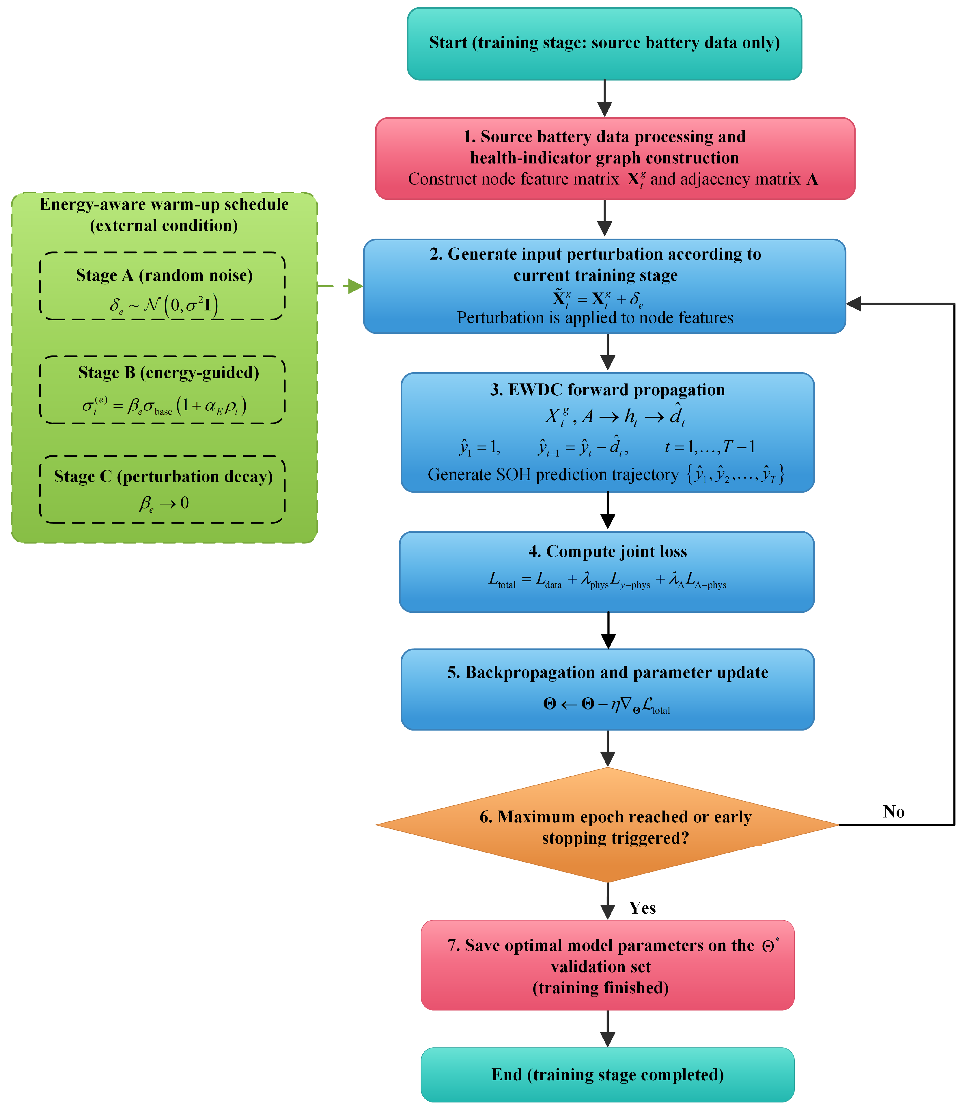
EWDC was trained using the three-stage strategy described in Section 2.4, with Stages A, B, and C corresponding to epochs 1–50, 51–300, and 301–500, respectively. The Adam optimizer was adopted, and the weights of the degradation-consistency constraints were adaptively adjusted during training. For all comparison models, the same partial-charge HI inputs, source/validation partitions, preprocessing procedure, and historical input information were used in each LOBO fold. All models were evaluated over ten independent runs, and architecture-specific hyperparameters were selected using the source validation data.

The main hyperparameter settings of EWDC are listed in

Table 3. Hyperparameter settings of EWDC on the two datasets.

Hyperparameter	Setting
Training epochs	500
Stage A	1–50
Stage B	51–300
Stage C	301–500
Batch size	32
Historical input-window length L	16
GCN hidden dimension	64
Dropout ratio	0.05
Learning rate	Stage A/B: $1\times {10}^{-4}$; Stage C: $5\times {10}^{-5}$
Feature-noise standard deviation	0.03
Initial constraint weights	${\lambda }_{\mathrm{phys}}^{min}=0.2,{\lambda }_{\Delta }^{min}=0.1$
Maximum constraint weights	${\lambda }_{\mathrm{phys}}^{max}=5.0,{\lambda }_{\Delta }^{max}=2.0$
SOH bounds	$y_{min}=0.40,y_{max}=1.05$
Degradation-increment bounds	$d_{min}=-0.03,d_{max}=0.03$

.

3.2. Overall LOBO Unseen-Cell Prediction Performance

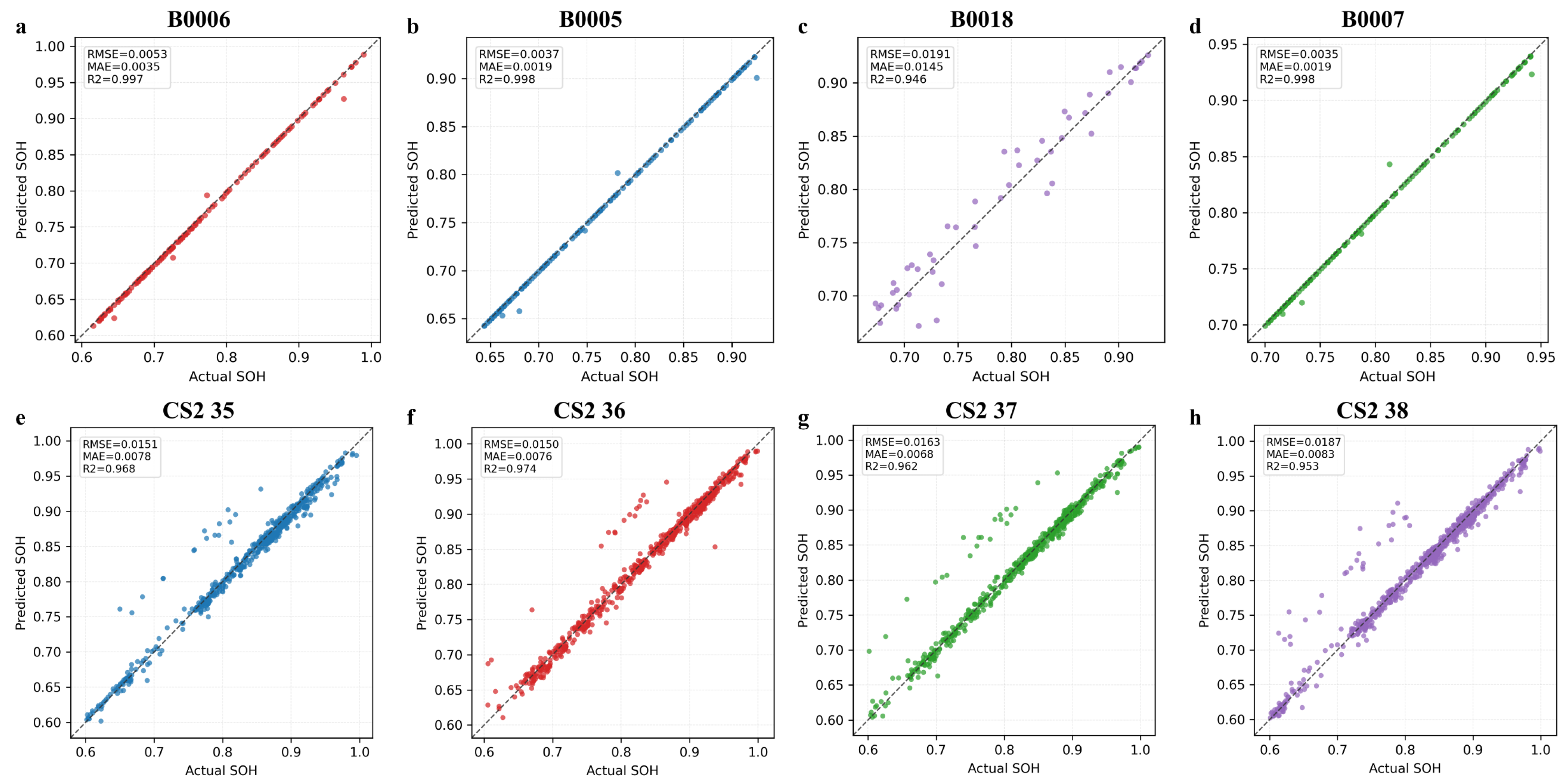
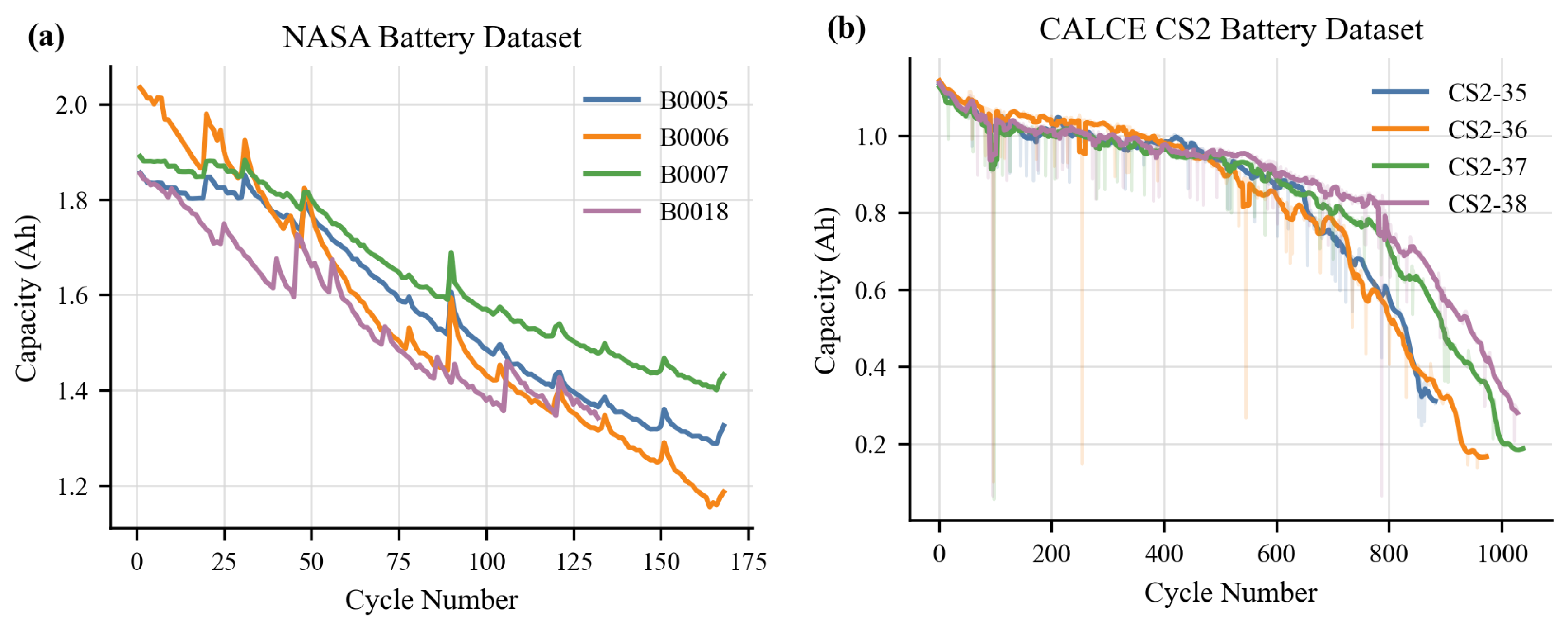
Figure 4 compares EWDC predictions with the ground-truth SOH for the eight target batteries. Most prediction points lie close to the ideal line $y=x$, indicating close agreement between predicted and ground-truth SOH. In the NASA dataset, the degradation trajectories of B0005, B0006, and B0007 were relatively smooth, and their prediction points were tightly clustered. By contrast, B0018 showed greater dispersion, reflecting a larger degradation mismatch between that battery and the source batteries. The CALCE-CS2 batteries had longer cycle sequences and more pronounced late-stage fading, resulting in somewhat greater dispersion of the predictions. Even so, the predictions remained close to the ideal line overall across both datasets.

In addition to the three external baselines, a basic graph–$\Delta$SOH configuration, denoted as None, was included to separate the effect of the underlying prediction architecture from the additional EWDC mechanisms. None retains the learnable HI graph, GCN encoder, signed degradation-increment prediction, and recursive SOH reconstruction, but excludes the energy-aware warm-up and degradation-consistency constraints.

TFT was included as an attention-based time-series baseline and has also been adopted in recent energy forecasting applications [35,36].

Table 4. SOH estimation results of EWDC and comparison models on the eight batteries.

Battery	RMSE/%					MAE/%					${\mathit{R}}^2$
	TCN	TFT	GNN	None	EWDC	TCN	TFT	GNN	None	EWDC	TCN	TFT	GNN	None	EWDC
B0006	1.62	1.45	1.36	1.48	0.53	1.13	1.03	0.90	1.03	0.35	0.948	0.956	0.966	0.966	0.997
B0005	1.50	1.36	1.25	0.93	0.37	1.04	0.94	0.82	0.59	0.19	0.942	0.968	0.972	0.980	0.998
B0007	1.48	1.34	1.22	1.19	0.35	0.98	0.88	0.76	0.83	0.19	0.956	0.979	0.976	0.970	0.998
B0018	3.15	3.27	2.43	3.65	1.91	2.55	2.21	1.95	2.92	1.45	0.872	0.903	0.919	0.887	0.946
CS2-35	2.65	2.21	1.90	2.15	1.51	1.72	1.41	1.11	1.25	0.78	0.901	0.932	0.948	0.935	0.968
CS2-36	2.48	2.05	1.82	3.05	1.50	1.54	1.25	1.05	1.85	0.76	0.915	0.941	0.955	0.920	0.974
CS2-37	2.74	2.35	2.02	2.58	1.63	1.52	1.20	0.91	1.42	0.68	0.884	0.916	0.939	0.918	0.962
CS2-38	3.05	2.62	2.26	3.95	1.87	1.72	1.38	1.05	2.07	0.83	0.865	0.902	0.927	0.898	0.953
Average	2.33	2.08	1.78	2.37	1.21	1.53	1.29	1.07	1.49	0.65	0.910	0.937	0.950	0.934	0.975

All values are means over ten independent runs. Run-wise RMSE distributions of TCN, TFT, GNN, and EWDC are shown in Figure 5. Bold values indicate the best prediction performance among the compared methods.

compares TCN [32], TFT [35,36], GNN [13], None, and EWDC on the eight held-out cells under the within-dataset LOBO protocol. Their average RMSE values were 2.33%, 2.08%, 1.78%, 2.37%, and 1.21%, respectively; the corresponding MAE values were 1.53%, 1.29%, 1.07%, 1.49%, and 0.65%, while the average $R^2$ values were 0.910, 0.937, 0.950, 0.934, and 0.975. EWDC achieved the best overall prediction accuracy among the compared configurations.

Among the external baselines, GNN achieved the best average performance. Relative to GNN, EWDC reduced the average RMSE and MAE by 32.19% and 38.83%, respectively. The comparison with GNN reflects the overall performance gain of the complete EWDC framework, while the contributions of individual components are examined separately in the subsequent ablation studies.

A battery-level paired Wilcoxon signed-rank test was further conducted between GNN and EWDC using the eight held-out batteries. EWDC significantly outperformed GNN for both RMSE and MAE ($p<0.01$ for both metrics), and the differences remained significant after Holm correction ($p_{\mathrm{adj}}<0.05$). This result indicates that the improvement was consistent across the target batteries rather than being driven by only a few individual cases.

Performance varied across the eight target batteries, with EWDC RMSE ranging from 0.35% to 1.91% and MAE from 0.19% to 1.45%. B0018 was the most challenging target, with an RMSE of 1.91%, an MAE of 1.45%, and an $R^2$ of 0.946, compared with the overall averages of 1.21%, 0.65%, and 0.975, respectively.

The basic graph–$\Delta$SOH configuration did not outperform the direct GNN baseline, indicating that the recursive graph–increment architecture alone was insufficient to achieve the final improvement. One possible reason is that local increment errors may accumulate during recursive reconstruction, whereas the additional training and consistency mechanisms in EWDC help stabilize this process.

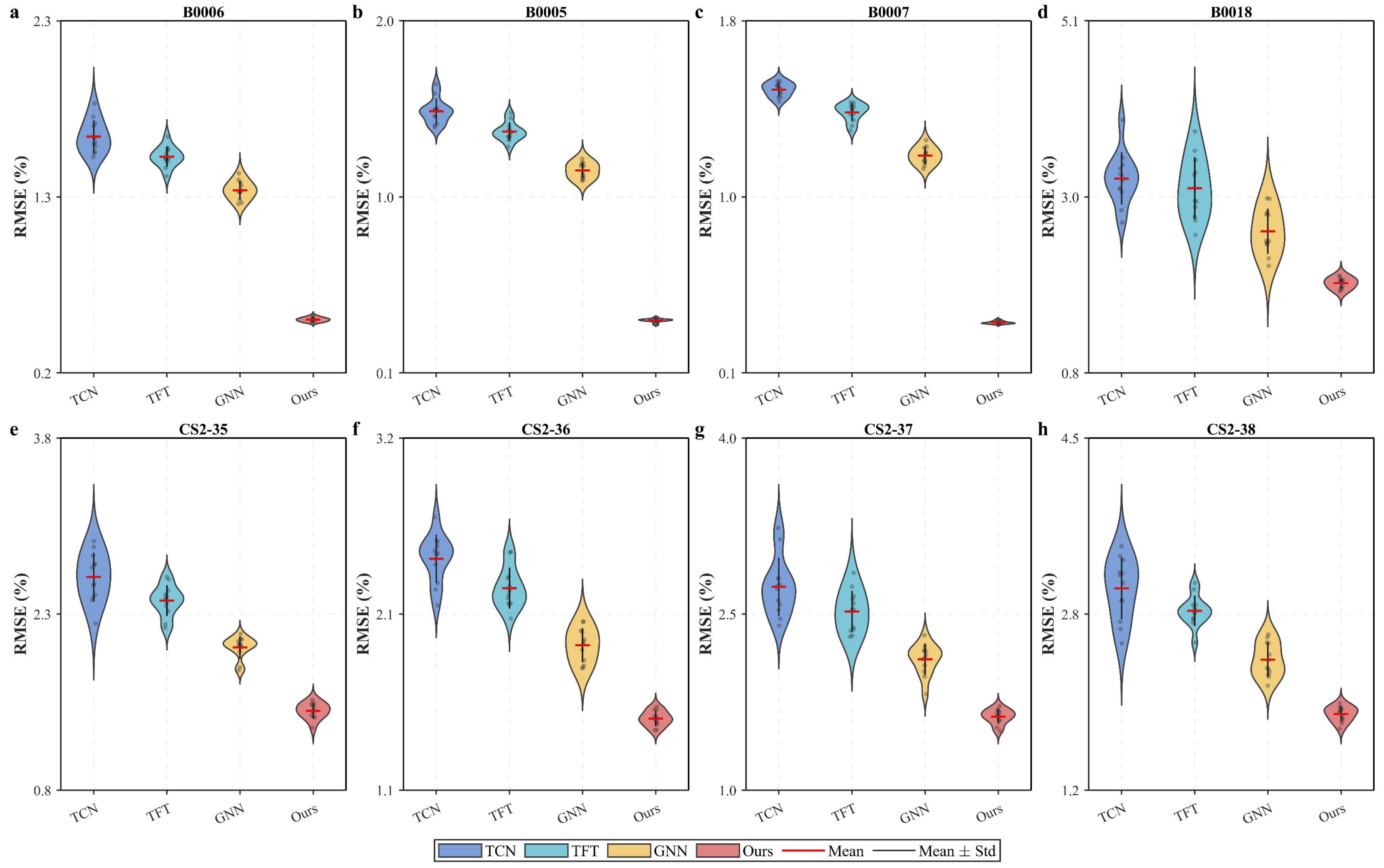
Figure 5 shows the repeated-run RMSE distributions of TCN, TFT, GNN, and EWDC. TCN and TFT exhibited relatively wide error distributions, especially on B0018 and the CALCE-CS2 batteries, where the run-to-run fluctuation was more pronounced. GNN reduced the overall error, but noticeable dispersion remained on batteries with complex degradation trajectories. EWDC yielded lower overall RMSE and a more concentrated error distribution, suggesting more stable optimization across repeated runs.

3.3. Within-Dataset Unseen-Cell Generalization Under Limited Source-Battery Conditions

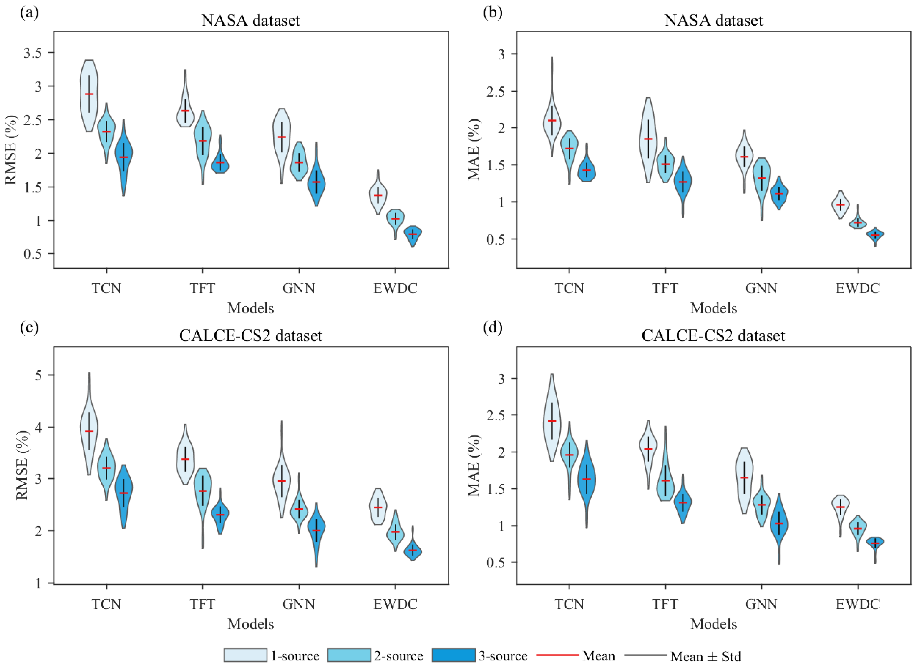
The number of source batteries directly affects the coverage of degradation patterns available for within-dataset unseen-cell prediction. To investigate model generalization when the number of training source batteries is limited, 1-source, 2-source, and 3-source experiments were conducted separately on the NASA and CALCE-CS2 datasets. For each dataset, one cell was selected as the target in each run, and the model was trained using one, two, or three source batteries from the same dataset, respectively. For the 1-source and 2-source settings, the reported values were averaged over all selectable source-battery combinations and therefore represent the overall behavior under each source-data condition rather than the result of a single favorable source selection. The 3-source setting corresponds to the standard LOBO protocol. The results are shown in

Table 5. Average prediction results of different models under limited-source-battery conditions.

Dataset	No. of Source Batteries	RMSE/%				MAE/%
		TCN	TFT	GNN	EWDC	TCN	TFT	GNN	EWDC
NASA	1-source	2.88	2.63	2.24	1.37	2.10	1.85	1.61	0.96
NASA	2-source	2.32	2.18	1.86	1.02	1.72	1.51	1.32	0.72
NASA	3-source	1.94	1.86	1.57	0.79	1.43	1.27	1.11	0.55
CALCE-CS2	1-source	3.92	3.38	2.96	2.45	2.42	2.04	1.65	1.25
CALCE-CS2	2-source	3.21	2.77	2.42	1.98	1.96	1.61	1.28	0.96
CALCE-CS2	3-source	2.73	2.31	2.01	1.63	1.63	1.31	1.03	0.76

Bold values indicate the best prediction performance among the compared methods.

and Figure 6.

As the number of source batteries increased from one to three, the RMSE and MAE of all models decreased overall, indicating that additional source batteries provided broader coverage of degradation patterns. However, the sensitivity to source-battery count differed across models. TCN and TFT showed larger errors when only a few source batteries were available, suggesting that local temporal patterns alone were insufficient to accommodate degradation differences in the target cell. GNN reduced the errors by modeling dependencies among health indicators, but its performance remained variable when the source-battery distribution changed substantially.

EWDC produced the lowest error under the 1-source, 2-source, and 3-source settings. Averaged over the six experimental groups, the RMSE values of TCN, TFT, GNN, and EWDC were 2.83%, 2.52%, 2.18%, and 1.54%, respectively, while the corresponding MAE values were 1.88%, 1.60%, 1.33%, and 0.87%. Figure 6 also shows a more concentrated error distribution for EWDC, suggesting more stable unseen-cell performance as the number of source batteries changed.

Among the limited-source settings, CALCE-CS2 with only one source battery was the most challenging condition for EWDC, yielding an RMSE of 2.45% and an MAE of 1.25%, compared with 1.63% and 0.76% under the corresponding 3-source setting.

These results indicate that increasing the number of source batteries provided richer degradation-pattern information for all models. Even so, EWDC consistently yielded lower and more concentrated prediction errors across different source-battery settings, which suggests stable within-dataset unseen-cell generalization under changes in training-data scale, including the limited-source-battery regime.

3.4. Effectiveness of the Energy-Aware Warm-Up Strategy

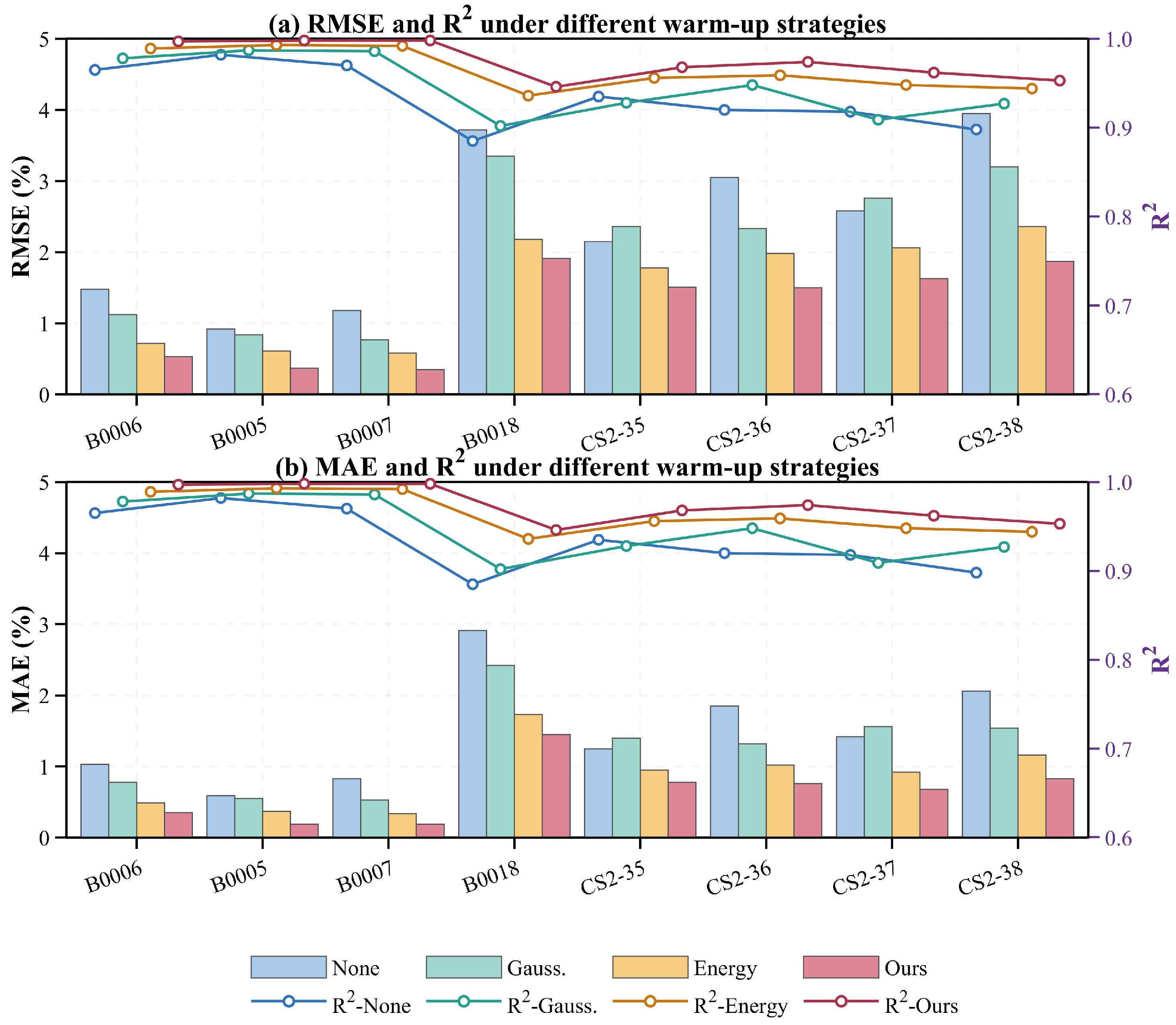
Based on the None configuration reported in Table 4, three additional training settings were compared to examine the effects of the warm-up and degradation-consistency mechanisms: Gauss., Energy, and Ours. Gauss. introduces uniform Gaussian perturbation, Energy further adjusts the perturbation magnitude according to the source-domain distribution-offset coefficient ${\rho }_i$, and Ours combines the energy-aware warm-up with the two-level degradation-consistency constraints. The remaining architecture and training settings were kept unchanged.

Figure 7 shows a stepwise performance improvement from None to Gauss., from Gauss. to Energy, and from Energy to Ours. The improvement from None to Gauss. indicates that generic input perturbation already provides a regularization benefit under limited-source training. Because Gauss. and Energy share the same prediction architecture, training budget, warm-up stages, base noise intensity, and decay schedule, their comparison isolates the effect of sample-dependent perturbation scaling. Introducing ${\rho }_i$-based scaling reduced the average RMSE and MAE by 26.66% and 30.89%, respectively, relative to uniform Gaussian perturbation. This improvement indicates that allocating stronger perturbation to relatively atypical source windows and weaker perturbation to central windows is more effective than applying a uniform perturbation magnitude under the present LOBO setting. The further improvement from Energy to Ours reflects the additional contribution of the two-level degradation-consistency constraints.

Overall, the ablation results show that sample-dependent perturbation provides a further improvement over uniform Gaussian noise under the present LOBO setting, while the degradation-consistency constraints contribute an additional performance gain. The distribution-offset coefficient is therefore interpreted as a source-domain sample-deviation measure rather than a direct estimate of source-to-target domain shift.

3.5. Effectiveness of the Degradation-Consistency Constraints

The degradation-consistency constraints are intended to suppress spurious SOH rebounds and abrupt changes in degradation increments that do not align with battery degradation behavior. To evaluate their effect, four ablation settings were evaluated under the same model structure and training strategy: without degradation-consistency constraints, SOH-trajectory-level constraints only, degradation-increment-level constraints only, and two-level degradation-consistency constraints. The results are listed in

Table 6. Ablation results for the degradation-consistency constraints.

Constraint Form	RMSE/%	MAE/%	${\mathit{V}}_{\mathbf{ER}}$	${\mathit{E}}_{\mathbf{trend}}(\times {10}^{-4})$
Without Consistency Constraints	1.53	0.82	0.184	8.62
SOH-Trajectory Constraints Only	1.54	0.74	0.171	7.37
$\Delta \mathrm{SOH}$-Increment Constraints Only	1.29	0.70	0.146	4.89
Two-Level Consistency Constraints	1.21	0.65	0.087	3.72

Bold values indicate the best prediction performance among the compared methods.

.

The ablation results indicate that the two types of degradation-consistency constraints played different roles. With only the SOH-trajectory-level constraints, the MAE, excessive-rebound violation rate, and trend-variation error all decreased, whereas the RMSE remained almost unchanged. This pattern suggests that these constraints mainly improved the local consistency of the predicted trajectory. With only the degradation-increment-level constraints, all metrics improved further, suggesting that constraining local degradation increments helped reduce both prediction error and trend deviation. The full two-level constraints produced the best overall result, indicating that jointly constraining the final SOH state and the trajectory-generation process reduced abnormal rebounds and local trend deviation more effectively.

Overall, the two-level constraints reduced trend deviation while preserving the local fluctuations observed in the measured capacity sequence. The state- and increment-level boundary terms further regulated the magnitude of reconstructed SOH states and cycle-to-cycle degradation changes, contributing to more stable trajectory generation.

3.6. Additional Ablation and Sensitivity Analysis

To further examine the role of health-indicator dependency modeling, the learned graph in EWDC was compared with no-graph and fixed Pearson-correlation alternatives while keeping the remaining model components and training settings unchanged. In the fixed-graph setting, the adjacency matrix was computed from the source training data of the current LOBO fold and kept fixed throughout training, with $A_{\mathrm{fixed}}(i,j)=\left|\mathrm{PearsonCorr}({\mathrm{HI}}_i,{\mathrm{HI}}_j)\right|$. In the no-graph setting, graph construction and GCN message passing were removed, while the remaining EWDC modules were retained.

As shown in

Table 7. Ablation results of the health-indicator graph construction.

Graph Setting	RMSE (%)	MAE (%)	${\mathit{R}}^2$
No Graph	1.54	0.88	0.962
Fixed Graph (Pearson)	1.34	0.72	0.971
Learned Graph (EWDC)	1.21	0.65	0.975

Bold values indicate the best prediction performance among the compared methods.

, introducing a fixed correlation graph reduced the RMSE from 1.54% to 1.34% and the MAE from 0.88% to 0.72% compared with the no-graph setting. The learned graph further reduced the RMSE and MAE to 1.21% and 0.65%, respectively, with an $R^2$ of 0.975. These results indicate that explicitly modeling dependencies among HIs improves degradation representation, while task-adaptive graph learning provides additional benefit over a fixed linear correlation structure.

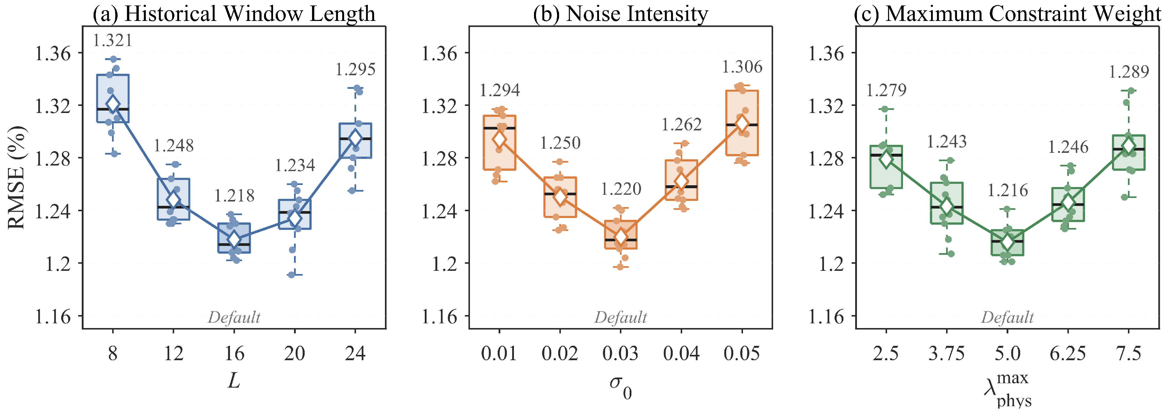
Sensitivity analyses were further conducted for the historical input-window length L, noise intensity ${\sigma }_0$, and maximum constraint weight ${\lambda }_{\mathrm{phys}}^{max}$, with each configuration evaluated over ten independent runs.

As shown in Figure 8, among the tested settings, the lowest mean RMSE values are obtained at $L=16$, ${\sigma }_0=0.03$, and ${\lambda }_{\mathrm{phys}}^{max}=5.0$, with corresponding RMSEs of 1.218%, 1.220%, and 1.216%, respectively. Performance degrades only moderately when these parameters deviate from their default settings, indicating that EWDC maintains relatively stable performance within the tested ranges.

The influence of the available charging information was further examined by progressively shortening the partial-charge observation window while keeping the feature definitions, model architecture, and training protocol unchanged, with the results summarized in

Table 8. Sensitivity of EWDC to the available partial-charge window.

Window (%)	CC Voltage (V)	CV Current (A)	RMSE (%)	MAE (%)	${\mathit{R}}^2$
50	4.10–4.20	0.50–0.30	1.61	0.91	0.956
75	4.05–4.20	0.50–0.20	1.42	0.75	0.968
100	4.00–4.20	0.50–0.10	1.21	0.65	0.975

Bold values indicate the best prediction performance among the compared methods.

. The original CC interval of 4.00–4.20 V and CV current-decay interval of 0.50–0.10 A were defined as the 100% setting, while the 75% and 50% settings used progressively shortened observation ranges.

As the available partial-charge window was shortened, the prediction error increased gradually. The RMSE increased from 1.21% under the full window to 1.42% and 1.61% under the 75% and 50% settings, respectively, while the corresponding MAE values increased from 0.65% to 0.75% and 0.91%. This trend indicates that a broader partial-charge observation range provides more complete degradation information for SOH prediction. Nevertheless, EWDC maintained an RMSE of 1.61% and an $R^2$ of 0.956 with only 50% of the baseline observation window, showing that shortened charging segments still retain useful degradation information.

3.7. Computational Cost Analysis

The computational costs summarized in

Table 9. Computational cost of different models.

Model	Parameters	Train Time (min/fold)	Inference (ms/cycle)	Peak Memory (MB)
TCN	85,440	5.8	0.12	15.2
TFT	342,120	12.5	0.45	48.6
GNN	45,216	4.2	0.14	18.5
None	56,832	5.1	0.16	22.4
EWDC	56,832	6.3	0.16	22.4

were evaluated on the NASA LOBO fold with B0018 held out as the target battery. All models were implemented in Python 3.10 with PyTorch 2.0.1 and tested on the same platform equipped with an Intel Core i7-14700K CPU and an NVIDIA RTX 4080 GPU with 16 GB of memory. Training time denotes the wall-clock time per fold, while inference time and peak GPU memory were measured with a batch size of one.

Compared with the architecture-matched None configuration, EWDC increased the training time from 5.1 to 6.3 min/fold, while the parameter count, inference latency, and peak memory remained unchanged. At the same time, the average RMSE decreased from 2.37% to 1.21%. This indicates that the additional computational cost of EWDC is mainly concentrated in offline training, while the deployed inference model does not introduce extra parameters, latency, or memory overhead relative to the architecture-matched configuration.

Compared with the external baselines, EWDC remains substantially lighter than TFT in terms of parameter count, inference latency, and memory usage, although it is slightly more demanding than the simpler GNN baseline. Therefore, the computational increase of EWDC can be regarded as moderate relative to the achieved prediction improvement. Nevertheless, the reported measurements were obtained on desktop GPU hardware, and deployment on resource-constrained BMS platforms still requires hardware-specific validation.

4. Conclusions

This study addressed prediction drift and trajectory instability in within-dataset unseen-cell SOH prediction under limited-source-battery conditions. EWDC was formulated as a coordinated framework that integrates health-indicator graph encoding, cycle-to-cycle degradation-increment prediction, recursive SOH-trajectory reconstruction, a three-stage energy-aware warm-up, and two-level degradation-consistency constraints for target-label-free unseen-cell prediction. Experiments on the NASA and CALCE-CS2 datasets showed that EWDC achieved average RMSE, MAE, and $R^2$ values of 1.21%, 0.65%, and 0.975, respectively, across eight target batteries. Relative to the GNN baseline, the average RMSE and MAE were reduced by 32.19% and 38.83%, respectively. The limited-source experiments and ablation studies further supported the contribution of the coordinated design to prediction accuracy and trajectory stability.

The current evaluation is limited to identifiable CC-CV partial-charge segments and within-dataset LOBO settings. Although the NASA and CALCE-CS2 datasets differ in cell configuration, chemistry, capacity, and operating conditions, they were evaluated as separate experimental domains; therefore, the present results do not establish direct cross-dataset generalization. The robustness of EWDC under substantial shifts in degradation patterns and operating protocols across datasets remains to be verified. In addition, both datasets employ relatively regular CC-CV charging, and the current HI extraction relies on predefined voltage and current segments. Substantial changes in charging current or temperature, irregular charging profiles, incomplete charging segments, or stronger measurement disturbances may alter the HI distributions and require further adaptation. Future work will therefore extend the evaluation to cross-dataset generalization and broader charging conditions, while further investigating dynamic HI relationships and adaptive training strategies.