IBT-PPO: A Dual-Stage Intelligent Forecasting and Reinforcement Learning Framework for Optimal Scheduling in Hybrid Renewable Energy Systems

Abstract

In this work, Intelligent Bidirectional Long Short-Term Memory with Temporal Fusion Transformer-based prediction and Proximal Policy Optimization (IBT-PPO) is proposed in response to the challenges of uncertain renewable generation, fluctuating demand, and inefficient energy scheduling in hybrid renewable energy systems. The algorithm is based on a dual-stage framework that integrates machine learning forecasting with reinforcement learning-based planning. Initially, a hybrid Bi-LSTM-TFT model is employed to generate accurate short-term forecasts of wind power, solar power, and demand, which employs temporal dependencies and multi-horizon patterns. After that, the PPO strategy is designed to optimize scheduling decisions, adaptively balancing battery usage, grid reliance, and renewable dispatch. To enhance robustness, adaptive feature weighting and temporal gating strategies are incorporated, ensuring stable convergence and reduced planning redundancy. Subsequently, the energy allocation is refined through iterative learning to minimize operational cost and maximize renewable penetration. The proposed framework is evaluated as an offline/post hoc forecasting and scheduling approach, with the Bi-LSTM–TFT module exploiting historical temporal representations and the PPO agent optimizing energy-management decisions based on the resulting forecasts. The experimental evaluation is carried out using the Open Power System Data (OPSD) dataset, which provides realistic time-series data for wind, solar, demand, and electricity prices. Thus, the IBT-PPO system integrates multi-horizon probabilistic forecasting and adaptive feature weighting for better prediction and planning accuracy and achieves a 24.1% cost reduction and 95.5% renewable utilization, thereby advancing efficient and intelligent energy prediction and planning.

1. Introduction

1.1. Background

The rising demand for energy solutions plays a significant role in hybridized renewable energy systems, which combine renewable energy sources, such as solar and wind, with energy storage and grid support [1]. Despite their growth, the uncertain nature of renewable generation and dynamic demand remains unpredictable, leading to difficulties in predicting and planning energy at a critical stage [2]. In terms of energy prediction, the research in [3] explores the use of machine learning for predicting building energy demands and renewable energy generation. The use of a deep reinforcement learning method for energy optimization [4] complements the Proximal Policy Optimization (PPO) used in this research to balance renewable energy, storage, and grid reliance. Weather data integration for accurate forecasting, as analyzed in [5], is another critical aspect that improves the accuracy of short-term forecasts for renewable generation.

The integration of solar and wind energy with storage systems, as explored in [6], highlights the role of machine learning in enhancing storage management—a crucial aspect of ensuring system reliability and sustainability. Furthermore, a hybridized machine learning model is proposed for solar irradiance forecasting, which has a direct influence on solar forecasting [7]. The storage optimization phase is enriched by investigating hydrogen-based storage for renewable energy systems, addressing economic and environmental uncertainties [8]. The focus on mitigating uncertainty in renewable generation, particularly in solar and wind systems, is a challenge addressed in this research, which is also tackled through RL [9]. The role of machine learning in enhancing solar energy prediction accuracy, as discussed in [10], further improves the forecasting approach in this research. In [11], optimizing multi-objective hybrid energy systems for improved stability and efficiency in energy integration involves balancing the optimization of cost, renewable energy usage, and system stability. The use of machine learning models helps to accurately forecast neighborhood-level energy balance by integrating renewables (such as solar and wind) into building energy consumption patterns, enabling more intelligent planning of hybridized renewable energy systems [12].

Hence, the use of machine learning and deep learning models enhances renewable energy forecasting by capturing complex generation patterns, for improving grid reliability and supporting grid management [13]. Earlier artificial neural network models analyzed data-driven models that can accurately forecast renewable energy outputs, such as solar, wind, and hydro systems, addressing the uncertainty of renewable sources [14]. By extending the simulated microgrid operations, predicting demand–supply dynamics, and optimizing intelligent grid scheduling for reliable and efficient energy delivery [15], the approach further enhances grid resilience by modeling battery health and incorporating fuel dynamics for adaptive scheduling under varying operational conditions [16]. For improved hourly solar irradiation prediction, the temporal fusion transformer [17] is employed, addressing the limitations of large-scale modeling and enhancing interpretability.

Forecasting-oriented approaches based on machine learning and deep learning [3,4,5,6,7,10,11,12,13,14,15,16] mainly focus on improving the prediction accuracy of solar power, wind power, or energy demand, but the generated forecasts are not systematically integrated with subsequent energy-dispatch decisions. Conversely, optimization and energy-management approaches [8,9,11,13] primarily focus on system configuration, storage utilization, or operational scheduling, while the uncertainty associated with renewable-generation forecasts is often represented using deterministic values or simplified assumptions. Thus, a clear research gap remains in the integrated treatment of probabilistic multi-horizon renewable forecasting, uncertainty-aware scheduling, risk-preference-based dispatch, and physically constrained battery management. Addressing this gap is essential for improving the robustness and practical feasibility of hybrid renewable-energy system operation under variable renewable generation and changing energy demand.

1.2. Novelty

Traditional methods often handle renewable-energy forecasting and scheduling as separate processes, limiting their ability to respond effectively to temporal variability and operational uncertainty. In contrast, the proposed IBT-PPO framework integrates a BiLSTM–TFT forecasting architecture with PPO-based adaptive energy scheduling. The BiLSTM component captures bidirectional sequential dependencies, while TFT performs variable selection, gated temporal transformation, and attention-based multi-horizon feature fusion to generate probabilistic renewable-generation forecasts. SHAP-based adaptive feature weighting further quantifies the contribution of meteorological, temporal, and historical variables and incorporates their relative importance into the forecasting representation. The PPO stage utilizes the resulting forecast information and uncertainty characteristics to adapt battery charge/discharge and renewable-energy dispatch decisions according to the defined operational objectives and constraints.

The specific novelty of IBT-PPO is established through the functional integration and complementary role of Bi-LSTM, TFT, and PPO, rather than through the individual use of these established techniques. The Bi-LSTM component extracts bidirectional temporal dependencies from historical renewable-generation and meteorological sequences, capturing short-term fluctuations and longer temporal patterns. The TFT component then performs interpretable variable selection, gated temporal processing, attention-based feature fusion, and multi-horizon probabilistic forecasting, generating renewable-power forecasts with uncertainty estimates. These forecast distributions are not treated as an isolated prediction output; the predicted renewable-generation profiles and associated uncertainty characteristics are transferred to the PPO scheduling stage as decision-relevant state information. PPO then learns an adaptive control policy for renewable-energy utilization, battery charging/discharging, and grid interaction under operating constraints and competing economic and renewable-utilization objectives. This creates a closed forecasting-to-decision pathway in which forecasting information directly influences sequential energy-management actions. The proposed integration is further distinguished from conventional hybrid deep learning models that focus primarily on improving prediction accuracy and from reinforcement learning approaches that generally operate with deterministic forecasts or raw measurements, without an uncertainty-aware, multi-horizon forecasting stage.

1.3. Main Contributions

The main contributions of the study are:

• Bi-LSTM, TFT, and PPO are integrated into an IBT-PPO framework to enhance renewable energy management by addressing the scheduling limitations of conventional models.
• Adaptive learning and uncertainty quantification are achieved through PPO combined with quantile forecasting, enabling reliable grid operation under variable renewable inputs.
• On a real-world OPSD dataset, IBT-PPO consistently outperforms the IDGC-RNN, CNN-LSTM, and GAN models, confirming robustness and scalability for intelligent grid forecasting.
• The proposed framework demonstrates superior prediction accuracy and renewable energy utilization compared with existing methods.

1.4. Paper Organization

The remainder of this research focuses on the following organization: Section 2 provides a comprehensive review of related works in intelligent energy prediction and planning, with a particular emphasis on hybridizing renewable energy factors. It critically discusses and analyzes each module of the energy forecasting and planning using the IBT-PPO model in Section 3. Experimental findings, comparative analysis with existing models, and performance analysis are also presented in Section 4. Section 5 concludes with a summary of the research idea, followed by a discussion of limitations and future enhancements.

2. Related Works

Singh et al. [18] make use of historical power and atmospheric statistics from several plants, train their models using K-Means clustering, and then use a hybrid deep learning model (a GRU-based RNN with mathematical models for PV, wind, and storage) to make predictions. The experimental results demonstrate that, in comparison to conventional models, the new ones are more accurate, have lower error rates, and exhibit greater connections among renewable sources. Generalization to real-world heterogeneous environments is hindered, nevertheless, by the study’s failure to adequately capture geographic variability and scalability across varied microgrids. Zafar et al. [19] presented a hybrid forecasting framework that uses meteorological and SCADA time-series data from three seasons to predict short-term PV and wind power using an Improved Dynamic Group-based Cooperative Optimization (IDGC) method in conjunction with radial basis function (RBF) network models. At 10 min and 1 h forecasting intervals, the model achieves better accuracy with less computing burden compared to classical NN and heuristic models. The limitations highlight the need for more efficient and scalable solutions for real-world microgrid deployment, including mitigating computational overhead from parallel training and reliance on high-quality meteorological data.

Mamodiya et al. [20] applied CNN-LSTM for forecasting and RL-based dual-axis tracking to increase energy yield by 41.4%, improve spectrum absorption by 18.7%, decrease RMSE from 57.3 to 31.6 W/m², lower panel temperature by 11.9 °C, and extend battery life by 60% through AI-driven storage and blockchain trading. Blockchain grid interoperability, long-term stability of perovskites, and scalability across continents are among the remaining gaps.

Alharbi and Iqbal [21] suggested a solar wind energy prediction framework that uses a combination of advanced ML/DL models, genetic algorithm-based feature selection, principal component analysis (PCA), and real-time ground and satellite inputs, along with historical meteorological and solar radiation datasets. The results demonstrated a considerable improvement in the accuracy of short-term forecasts and a decrease in RMSE. The data source struggles to work with sparse or poor-quality datasets, and it is also ineffective in predicting cloud-induced oscillations, the consequences of long-term degradation, and the lack of grid dynamics integration for comprehensive energy planning. Qiu and Entchev [22] employed real-world energy demand and resource facts from remote Canadian villages to construct an optimization-based system that can design and simulate HRES configurations incorporating PV, wind, biomass, and batteries. The optimum configurations found have NPCs between $4.17 million and $8.68 million, LCOEs between $0.33 and $0.69 per kilowatt-hour, and a yearly generation of 824,152 kilowatt-hours (kWh), with 59% biomass, 9% solar, and 32% wind. Modeling resource variability over the long term, integrating predicted demand, and making HRES planning scalable across varied remote geographies are all areas where research is lacking.

To maximize the efficiency of PV-grid operations, Gu et al. [23] utilized a dual-phase optimization algorithm. Realistic scenario synthesis is made possible by training the model using an 8760-hourly record dataset of solar irradiance, temperature, and residential load demand from varied climatic locations that spans an entire year. The system achieves 96% efficiency, a 20% cost reduction, and a 30% reduction in emissions. Additionally, downtime has been reduced from 120 to 60 h. However, there is a research gap in ensuring diversity, generalizability, and physical feasibility in energy scenario generation due to challenges like GAN mode collapse, dependence on large high-quality datasets, and a lack of physics-informed constraints.

Alhussan et al. [24] suggested that combining material optimization with intelligent control strategies can significantly enhance the electrical and thermal efficiency of hybrid solar energy systems, utilizing geometric optimization and adaptive fuzzy logic control. To maximize energy extraction, integrated passive and active strategies have the potential to reduce the thickness of the Tedlar layer. It improved electrical efficiency from 11.81% to 13.81% and thermal efficiency from 27% to 81%. There is a lack of research on predictive AI-driven planning and energy management methods that can optimize grid- or community-scale hybrid renewable systems, despite the effectiveness of these optimizations at the system level, which has concentrated chiefly on control and material improvements. Abdelsattar et al. [25] examined six ML algorithms: CatBoost, GBM, MLP regressor, SVM, XGBoost, and RF with the utilization of 4213 records of solar power generation. XGBoost has excellent performance on the test set, while RF achieves the highest R² (0.940 total, 0.971 training, and 0.818 test). While SVM and MLP struggled to generalize, the results showed that RF and XGBoost were the most stable and accurate for real-world forecasting. Nevertheless, there is a dearth of studies on the following topics: the effects of weather and seasons on solar power predictions, the absence of investigation into hybrid models, and the diversity of datasets.

Saxena et al. [26] presented a deep learning-driven methodology for real-time load forecasting and renewable energy production in power grids, utilizing advanced fractional extended state observer-based linear active disturbance rejection control (TD-FLADRC) for adaptive inertia regulation. The case study utilizes the New England IEEE 39-Bus Power System, demonstrating enhanced frequency regulation and grid stability through simulations and hardware-in-the-loop (HIL) experimental validation. Nonetheless, the study is constrained by its dependence on simulated data, especially in mitigating communication delays and facilitating multi-objective regulation through deep reinforcement learning. A power forecasting method for hybrid renewable energy systems called DeepFore is proposed by Pradeep et al. [27]. It uses WRF simulations to forecast wind farm production. The model optimizes features with TLBO after preprocessing the data with K++ clustering for anomaly detection. An improved use of wind power is predicted using Deep SARSA, a deep reinforcement learning system. The primary area that requires further investigation is how to scale the model to accommodate regionally varied renewable energy systems.

Wang et al. [28] optimized the hybrid building energy systems, with a focus on thermal comfort, energy cost reduction, and solar PV self-consumption, utilizing a multi-stage PPO framework that incorporates Imitation Learning (IL). The model, which has been tested with real-world ZEH data, increases interior temperature by 1.33 °C while improving energy self-sufficiency (34.86% in cold weeks and 46.10% in warm weeks) and self-consumption (15.78% in cold weeks and 18.47% in warm weeks). While the results are encouraging, scalability issues arise when using a reduced-order RC network.

Ibrahim et al. [29] investigated the application of electrochromic glazing (ECG) for improving energy efficiency in educational buildings under different climatic conditions. The study evaluated building performance across Alexandria, Hurghada, Asyut, and Cairo using energy simulations integrated with ASHRAE-based requirements. The results demonstrated energy savings of up to 9.20% in Alexandria, while the economic performance of ECG varied considerably among the investigated locations, with the reported levelized cost of savings reaching $0.629/kWh in Alexandria and $1.616/kWh in Hurghada. The study also demonstrated corresponding reductions in carbon emissions, emphasizing the influence of climatic conditions and adaptive building-envelope technologies on energy demand and environmental performance.

Hu et al. [30] proposed a hybrid data-driven framework integrating Temporal Fusion Transformer (TFT) and Soft Actor–Critic (SAC) for optimal scheduling of building-integrated energy systems. TFT was employed to forecast renewable generation and energy demand, while SAC was used to address the nonlinear scheduling problem. The study demonstrated that integrating temporal forecasting with continuous-control reinforcement learning improves energy-cost performance and computational efficiency, while also providing generalization and sensitivity analyses. This work provides a closely related benchmark for integrated forecasting and reinforcement learning-based energy scheduling. Huang and Yin [31] developed a Transformer–Soft Actor–Critic (T-SAC) framework for economic generation control in integrated energy systems with high renewable penetration. The Transformer architecture was incorporated into both the actor and critic networks to improve temporal feature extraction, while SAC provided adaptive control under changing system conditions. The framework was evaluated in multi-area integrated energy systems and demonstrated improved control performance under renewable-generation variability.

Listed in

Table 1. Comparative analysis of existing prediction and planning approaches in hybrid renewable energy systems.

Ref.	Dataset Usage	Model Used	Forecasting Capability	Planning Integration/ Applicability/ Uncertainty Handling/ Energy Storage Management	Results Achieved	Identified Gaps
Singh et al. [18]	Historical power, atmospheric data	GRU-based RNN + mathematical models	Short-term forecasts for PV, wind	✓/✗/✗/✓	More accurate predictions with lower error rates than conventional models	Limited scalability, geographic generalization issues
Zafar et al. [19]	Meteorological & SCADA data	IDGC + RBF network	10 min & 1 h forecasts	✓/✗/✗/✗	Better accuracy with reduced computing load vs. classical methods	Needs scalable, efficient solutions
Mamodiya et al. [20]	CNN-LSTM inputs	CNN-LSTM + RL	Improved forecasts	✓/✓/✗/✓	Energy yield up by 41.4%, absorption by 18.7%, RMSE lowered by 45%, panel temp reduced, battery life extended by 60%	Grid interoperability, stability, and scalability issues
Alharbi & Iqbal [21]	Satellite & ground data	ML/DL + GA + PCA	Short-term forecasts	✗/✓/✗/✗	Considerable accuracy improvement, lower RMSE	Sparse data limitations, cloud oscillations, and missing grid dynamics
Qiu & Entchev [22]	Remote village energy data	Optimization system	Demand forecasting	✓/✗/✗/✓	NPCs between $4.17–8.68 M, LCOEs $0.33–0.69/kWh, generation 824 kWh/year	Long-term variability & scalability are lacking
Gu et al. [23]	8760 h dataset	Dual-phase optimization	Seasonal load forecasting	✓/✓/✗/✗	96% efficiency, 20% cost reduction, 30% emission cut, downtime halved	Diversity, physics-informed modeling gaps
Alhussan et al. [24]	Material data	Geometric + fuzzy logic	Not the primary focus	✗/✗/✗/✓	Electrical efficiency improved from 11.81% to 13.81%, thermal efficiency from 27% to 81%	Predictive AI methods are absent
Abdelsattar et al. [25]	4213 records	ML (CatBoost, RF, etc.)	Forecasting stability	✗/✓/✗/✗	RF R2 of 0.940 total, 0.971 training, 0.818 test	Seasonal/weather impacts not studied
Saxena et al. [26]	IEEE bus data	Deep learning + TD-FLADRC	Real-time forecasting	✓/✓/✗/✗	Enhanced frequency regulation & stability	Simulation-only, lacks communication robustness
Pradeep et al. [27]	WRF simulations	Deep SARSA + TLBO	Wind power forecasts	✓/✗/✗/✗	Improved wind power usage predictions	Regional scalability issues
Wang et al. [28]	Building data	Multi-stage PPO + IL	Energy management forecasting	✓/✓/✗/✓	Interior temp improved by 1.33 °C, energy self-sufficiency 34.86–46.10%,	Scalability concerns

is a thorough summary of current research in energy forecasting and planning, with an emphasis on how datasets are used; the models; the forecasting abilities; and essential features, including real-time use, addressing uncertainty, and managing energy storage. Most previous research has focused on enhancing accuracy, efficiency, or storage optimization, but it does not concurrently address uncertainty quantification and real-time decision-making (Singh et al. [18]; Mamodiya et al. [20]; Gu et al. [23]). Numerous models rely on historical or generated information yet lack scalable solutions for heterogeneous environments (Zafar et al. [19]; Pradeep et al. [27]). In addition, forecasting results are not yet linked to planning frameworks, especially for uncertainty and grid interactions (Alharbi & Iqbal [21]; Saxena et al. [26]). The IBT-PPO model solves these issues by combining multi-horizon forecasting and planning. Quantile loss for uncertainty-aware forecasting provides real-time flexibility for renewable energy storage and grid management. IBT-PPO-based planning optimizes energy storage and dispatch in real time, unlike prior methods. Adaptive feature selection, used for scalability in varied situations, helps to complete the technique, thus addressing past research difficulties by ensuring scalability, prediction accuracy, and effective installation and use of renewable energy systems.

3. Research Methodology

The IBT-PPO goal is to create an intelligent system that anticipates energy supply and demand and optimizes scheduling to maximize renewable energy utilization and save expenses. The planning module, PPO, optimizes the energy system’s operational strategy using probabilistic forecasts from the combined BiLSTM + TFT for wind, solar load, and other factors. PPO outputs like battery charge/discharge and grid interaction decision lead the intelligent energy system toward cost reduction, renewable utilization, and grid integration. The IBT-PPO system makes forecast-informed decisions to improve storage efficiency and reduce grid dependence by adapting to changing conditions and uncertainties. The PV and wind units are constrained by their rated generation capacities and available renewable power at each time step. The battery-storage system is characterized by its nominal energy capacity, 20–100% SOC operating range, charging and discharging power limits, and corresponding charging and discharging efficiencies. The power converter is operated within its rated power capacity and conversion-efficiency limits. Grid interaction is constrained by the specified import and export power limits. The system power balance is maintained among PV generation, wind generation, battery charging/discharging, grid exchange, and load demand at every scheduling interval.

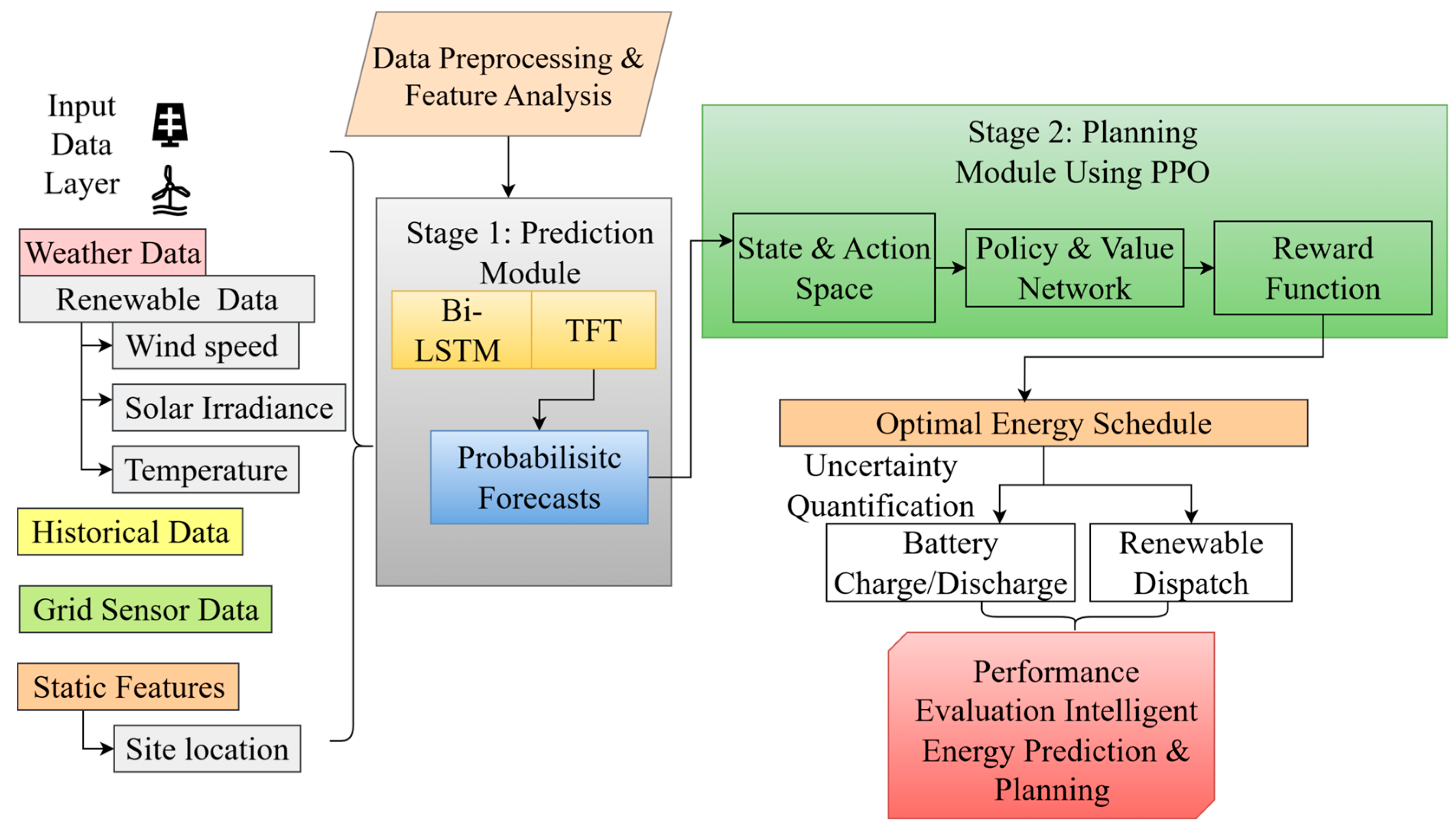
The IBT-PPO system has two stages, prediction and planning, as shown in Figure 1, supporting the integration of Bi-LSTM and TFT to identify temporal dependencies and uncertainty in projections for wind, solar, and demand. In Stage 1, a hybrid prediction module that combines Bi-LSTM and TFT makes probabilistic projections for wind, solar, and demand. In Stage 2, a planning module based on PPO sets the state-action space, improves policies using policy-value networks, and uses a reward-driven technique for adaptive energy management. The optimal energy plan that emerges from this ensures that the battery charges and discharges efficiently and that renewable energy is sent out when needed. Finally, performance evaluation demonstrates that the system is accurate, can handle a large amount of data, and can respond to changes for hybrid renewable energy systems. Then, reinforcement learning based on PPO makes the best scheduling rules for storage and grid interaction.

To prevent future-information leakage, the Bi-LSTM forecasting input is strictly restricted to observations available before the forecasting origin. For a forecasting time $t$, the input sequence is defined as $X_{t-L+1:t}$, where $L$ denotes the historical look-back window, while the prediction target corresponds to a future time $t+h$, $h>0$. The forward and backward LSTM units therefore operate only within this historical window; the backward unit processes the available sequence in reverse order but does not access observations from the future forecasting horizon. The target-period observations are excluded from both feature construction and model input. Chronological train, validation, and test partitions are maintained to preserve temporal ordering, and normalization and feature-weighting parameters are derived exclusively from the training data before application to subsequent periods.

The dataset is divided chronologically to preserve the natural temporal order of renewable-generation and energy-demand observations, with the earliest 70% of the time-series data assigned to training, the subsequent 15% to validation, and the final 15% to testing. No random shuffling is performed across these temporal partitions. All preprocessing parameters, including normalization and SHAP-based feature-weighting coefficients, are derived exclusively from the training period and subsequently applied to the validation and testing periods. For each forecasting instance, the input sequence contains only observations available to the forecasting origin $t$, $X_{t-L+1:t}$, while the target corresponds to a future horizon $t+h$. Validation and test observations are therefore excluded from model fitting and feature construction, preventing future-period information from entering the training process.

3.1. Data Exploration

To accurately anticipate renewable energy generation, data preparation and feature analysis are performed before model development. The raw wind speed, solar irradiance, temperature, and load data are normalized to reduce scale-related bias during model training. Missing observations are handled using linear interpolation, while the interquartile range (IQR) method is applied to identify and treat anomalous observations. For noise attenuation, a median filtering operation is applied to suppress isolated disturbances while preserving the temporal characteristics of the renewable-generation signals. A moving-average smoothing filter is subsequently applied to reduce residual short-term fluctuations and obtain a stable temporal representation. Pearson’s correlation coefficient ρ is used to quantify linear associations among the input variables, while autocorrelation analysis identifies temporal dependencies in electricity demand. The variable selection network (VSN) assigns data-driven importance to the input variables through its SoftMax-based selection mechanism, enabling relevant features to receive greater representation during temporal modeling. The processed data are subsequently supplied to the BiLSTM–TFT forecasting module for learning long-term dependencies and multi-horizon temporal patterns. This preprocessing and feature-analysis sequence provides a consistent input representation for probabilistic forecasting and subsequent PPO-based energy scheduling.

As provided in

Table 2. Data features for hybrid renewable energy systems.

Dataset	Feature	Description
Wind and Solar Power Generation [32]	Wind Speed	Wind speed data (m/s).
	Air Density	Air density data (kg/m3).
	Temperature	Temperature data (°C).
	Solar Irradiance	Ground and atmospheric irradiance data (W/m2).
	Photovoltaic Power Generation	Power generation from photovoltaic systems (kW or MW).
Open Power System Data (OPSD) [33]	Wind Power Generation	Hourly wind power generation data (kW or MW).
	Solar Power Generation	Hourly solar power generation data (kW or MW).
	Electricity Demand	Hourly demand data for electricity (kW or MW).
	Electricity Prices	Hourly electricity price data (€/MWh).
	Grid Power Consumption	Power consumption from the grid (kW or MW).
	Battery Storage Data	Data on battery storage and usage (kWh).

, the wind and solar power generation dataset offers meteorological and power generation data essential for accurate short-term forecasting of wind and solar generation, including wind speed, solar irradiance, and the resulting power outputs. These features are crucial for understanding the variability and availability of renewable energy sources. On the other hand, the OPSD dataset provides critical information regarding electricity demand, price fluctuations, and grid consumption, which are necessary for optimizing the dispatch and storage of renewable energy using RL. By combining these datasets, the model predicts and optimizes energy planning and scheduling, enhancing the integration of renewable energy into power grids while minimizing operational costs.

The PPO state and action spaces are explicitly defined to represent the operational condition of the hybrid renewable-energy system. At each decision interval $t$, the state vector comprises the predicted solar and wind power profiles, current battery state of charge (SOC), load demand, grid power exchange, and relevant temporal and operating variables. The action vector consists of the battery charging/discharging command and grid power exchange, with the renewable-generation dispatch determined according to the available renewable power and system demand. The battery SOC is constrained within 20–100%, while charging and discharging power are restricted to the rated battery limits and mutually exclusive operating modes are enforced. The battery state transition is governed by the charging/discharging efficiencies and the corresponding power command, ensuring SOC feasibility at every time step. Grid interaction is constrained by the specified grid import/export capacity, with power-balance constraints enforced between renewable generation, battery operation, grid exchange, and load demand. Actions violating battery or grid operating limits are clipped or penalized through the PPO reward function.

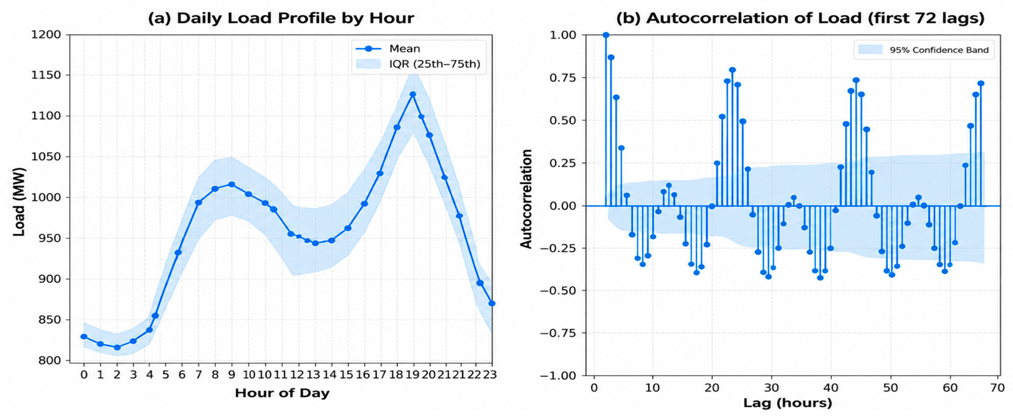
Figure 2 presents the temporal characteristics of electricity demand through the hourly load profile and autocorrelation analysis. The mean load exhibits pronounced intraday variability, with elevated demand during the morning and evening periods, while the interquartile range indicates greater dispersion during high-demand intervals. The autocorrelation profile shows significant dependence on multiple temporal lags, confirming the persistence and periodicity of electricity demand. These temporal characteristics justify the inclusion of historical load and time-dependent variables in the multi-horizon forecasting model.

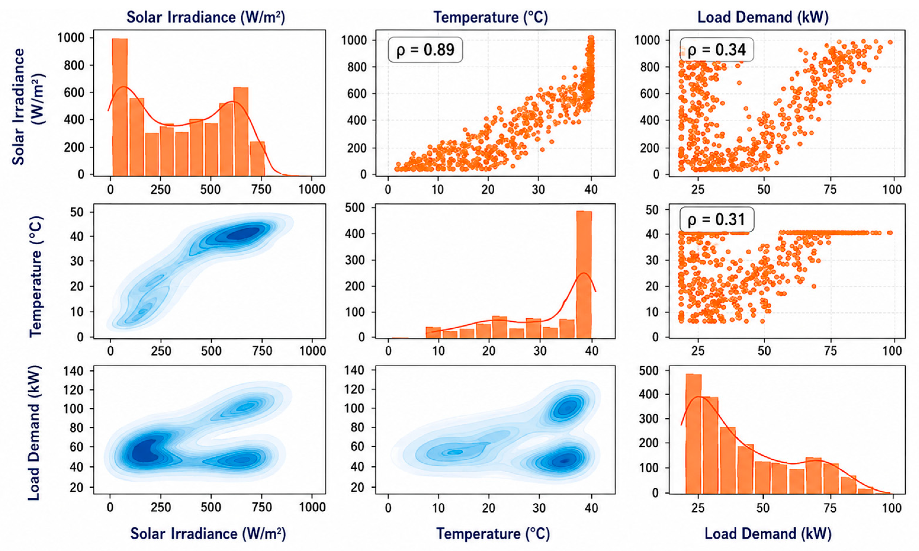
Figure 3 illustrates the statistical relationships between solar irradiance, temperature, and load demand. Solar irradiance and temperature exhibit a strong positive correlation ($\rho =0.89$), reflecting their common dependence on diurnal and seasonal conditions. Load demand exhibits comparatively weaker and nonlinear relationships with the environmental variables, indicating that electricity demand is influenced by multiple interacting factors. These relationships support the inclusion of meteorological and historical demand variables as explanatory features for solar generation and load forecasting.

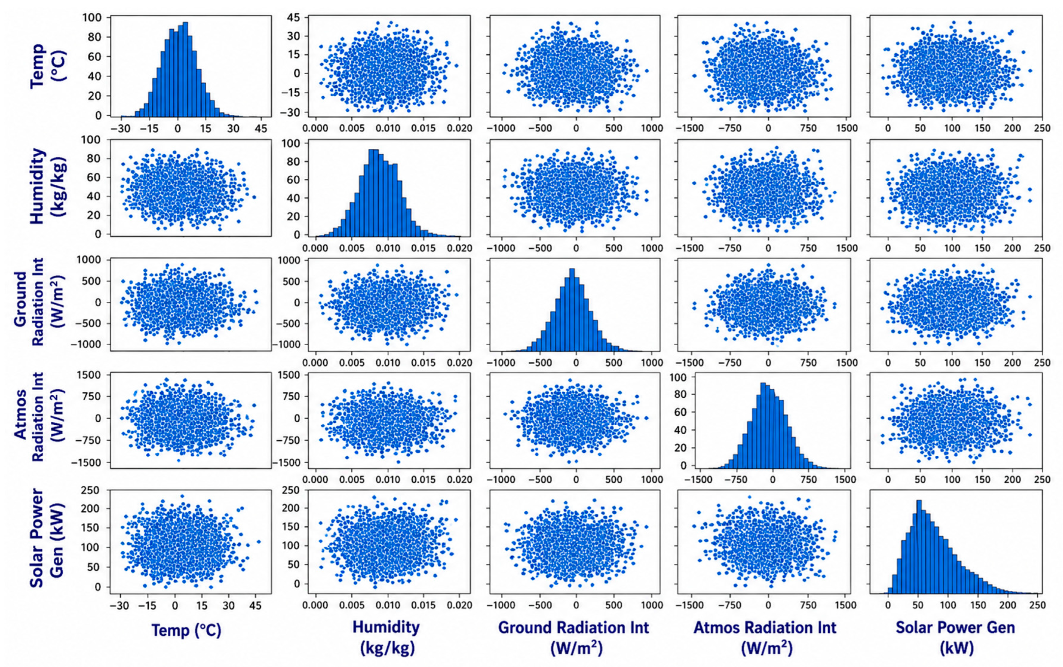
Figure 4 summarizes the distributions and pairwise relationships among temperature, humidity, ground radiation intensity, atmospheric radiation intensity, and solar power generation. The distributions indicate substantial variability in environmental conditions, while the scatter patterns reveal nonlinear relationships among several explanatory variables. The observed variability highlights the influence of meteorological conditions on solar-generation behavior and supports the use of multivariate temporal features in the BiLSTM–TFT forecasting architecture.

3.2. Stage 1: Hybrid Prediction Module Using Bi-LSTM and TFT

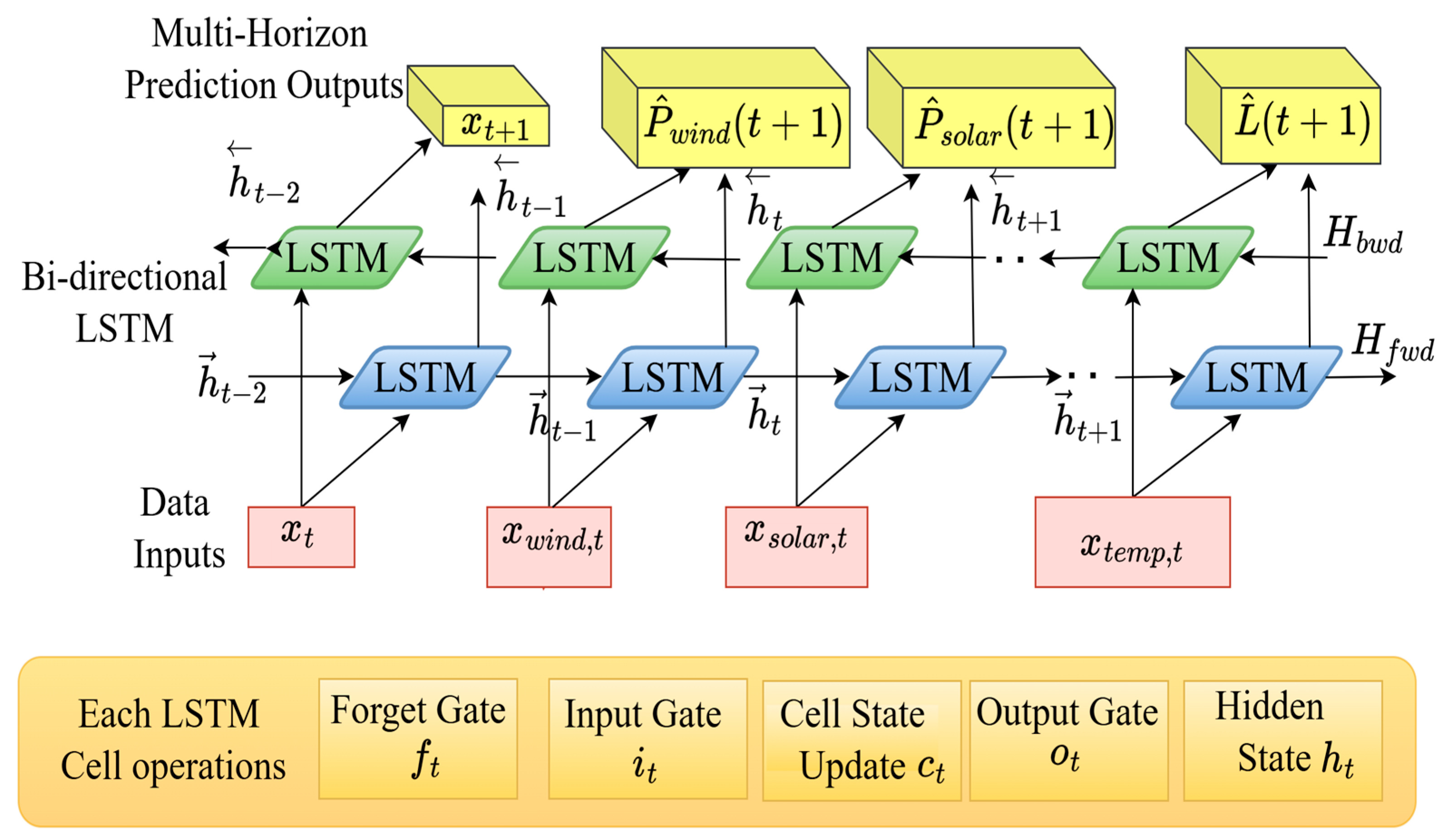
The proposed IBT-PPO system ensures that the use of Bi-LSTM efficiently models temporal dependencies. At the same time, adaptive feature selection and attention mechanisms enhance robustness against noise and uncertainty, enabling accurate and reliable renewable energy forecasting. The inputs at time step $\mathrm{t}$ are ${\mathrm{x}}_{\mathrm{t}}=\left[{\mathrm{x}}_{\mathrm{w}\mathrm{i}\mathrm{n}\mathrm{d},\mathrm{t}},{\mathrm{x}}_{\mathrm{s}\mathrm{o}\mathrm{l}\mathrm{a}\mathrm{r},\mathrm{t}},{\mathrm{x}}_{\mathrm{t}\mathrm{e}\mathrm{m}\mathrm{p},\mathrm{t}}\right]$ The module starts with the forget gate ${\mathrm{f}}_{\mathrm{t}}$ deciding which past data from historical wind speed or solar irradiance should be discarded in light of the most recent inputs from the cell state ${\mathrm{c}}_{\mathrm{t}-1}$ long-term memory to adapt to new inputs. The purpose of this gate is to control how much of the previous energy generation information, such as past wind speed or solar irradiance, is retained for future predictions. The use of $\mathsf{\sigma }$ sigmoid function squashes the output between 0 and 1, and ${\mathrm{W}}_{\mathrm{f}}$ as a weight matrix for the forget gate, controlling the influence of previous hidden states and current inputs for both forward and backward LSTM. The forward LSTM ${\mathrm{H}}_{\mathrm{f}\mathrm{w}\mathrm{d}}\leftarrow \mathrm{B}\mathrm{i}\mathrm{L}\mathrm{S}\mathrm{T}\mathrm{M}\_\mathrm{f}\mathrm{o}\mathrm{r}\mathrm{w}\mathrm{a}\mathrm{r}\mathrm{d}\left({\mathrm{X}}_{\mathrm{d}\mathrm{y}\mathrm{n}}\right)$ learns patterns from the past to future; likewise, the backward LSTM learns patterns from the future to the past using ${\mathrm{H}}_{\mathrm{b}\mathrm{w}\mathrm{d}}\leftarrow \mathrm{B}\mathrm{i}\mathrm{L}\mathrm{S}\mathrm{T}\mathrm{M}\_\mathrm{b}\mathrm{a}\mathrm{c}\mathrm{k}\mathrm{w}\mathrm{a}\mathrm{r}\mathrm{d}\left(\mathrm{r}\mathrm{e}\mathrm{v}\mathrm{e}\mathrm{r}\mathrm{s}\mathrm{e}\right({\mathrm{X}}_{\mathrm{d}\mathrm{y}\mathrm{n}}\left)\right)$. Thus, it follows ${\mathrm{H}}_{\mathrm{B}\mathrm{i}-\mathrm{L}\mathrm{S}\mathrm{T}\mathrm{M}}\leftarrow \mathrm{C}\mathrm{o}\mathrm{n}\mathrm{c}\mathrm{a}\mathrm{t}({\mathrm{H}}_{\mathrm{f}\mathrm{w}\mathrm{d}},{\mathrm{H}}_{\mathrm{b}\mathrm{w}\mathrm{d}})$ for processing temporal dependencies in both the forward and backward directions. The previous hidden state at time ${\mathrm{h}}_{\mathrm{t}-1}$ contains memory of past energy generation (wind and solar). ${\mathrm{x}}_{\mathrm{t}}$ represents the current input at time $\mathrm{t}$ represents features such as wind speed ${\mathrm{x}}_{\mathrm{w}\mathrm{i}\mathrm{n}\mathrm{d},\mathrm{t}}$ in m/s, solar irradiance ${\mathrm{x}}_{\mathrm{s}\mathrm{o}\mathrm{l}\mathrm{a}\mathrm{r},\mathrm{t}}$ in W/m², and temperature ${\mathrm{x}}_{\mathrm{t}\mathrm{e}\mathrm{m}\mathrm{p},\mathrm{t}}$ in °C, followed by a bias term ${\mathrm{b}}_{\mathrm{f}}$ of the forget gate.

The input gate ${\mathrm{i}}_{\mathrm{t}}$ controls how much new information from the current input ${\mathrm{x}}_{\mathrm{t}}$ wind speed and solar irradiance are added to the cell state, as shown in Figure 5. This enables the model to incorporate current features into its memory, which is crucial for generating accurate future forecasts. The weight matrix ${\mathrm{W}}_{\mathrm{i}}$ for the input gate controls the influence of both the hidden state and the current input. The ${\overrightarrow{\mathrm{h}}}_{\mathrm{t}}$ at each time step is given as ${\mathrm{L}\mathrm{S}\mathrm{T}\mathrm{M}}_{\mathrm{f}\mathrm{o}\mathrm{r}\mathrm{w}\mathrm{a}\mathrm{r}\mathrm{d}}\left({\mathrm{X}}_{\mathrm{t}},{\overrightarrow{\mathrm{h}}}_{\mathrm{t}-1}\right)$, and ${\overleftarrow{\mathrm{h}}}_{\mathrm{t}}$ gives the ${\mathrm{L}\mathrm{S}\mathrm{T}\mathrm{M}}_{\mathrm{b}\mathrm{a}\mathrm{c}\mathrm{k}\mathrm{w}\mathrm{a}\mathrm{r}\mathrm{d}}\left({\mathrm{X}}_{\mathrm{t}},{\overleftarrow{\mathrm{h}}}_{\mathrm{t}+1}\right)$ the ability to regulate the information flow by applying gating mechanisms ${\mathrm{h}}_{\mathrm{t}}=\left[{\overrightarrow{\mathrm{h}}}_{\mathrm{t}};{\overleftarrow{\mathrm{h}}}_{\mathrm{t}}\right]$. The input gate uses both the hidden state and current input to determine the amount of information from the input solar irradiance at time $\mathrm{t}$ that influences the model’s memory, with ${\mathrm{b}}_{\mathrm{i}}$ as the bias term for the input gate as given in Equations (1)–(5).

$${\mathrm{f}}_{\mathrm{t}}=\mathsf{\sigma }\left({\mathrm{W}}_{\mathrm{f}}·\left[{\mathrm{h}}_{\mathrm{t}-1},{\mathrm{x}}_{\mathrm{t}}\right]+{\mathrm{b}}_{\mathrm{f}}\right)$$

(1)

$${\mathrm{i}}_{\mathrm{t}}=\mathsf{\sigma }\left({\mathrm{W}}_{\mathrm{i}}·\left[{\mathrm{h}}_{\mathrm{t}-1},{\mathrm{x}}_{\mathrm{t}}\right]+{\mathrm{b}}_{\mathrm{i}}\right)$$

(2)

$${\mathrm{c}}_{\mathrm{t}}={\mathrm{f}}_{\mathrm{t}}·{\mathrm{c}}_{\mathrm{t}-1}+{\mathrm{i}}_{\mathrm{t}}·\mathrm{t}\mathrm{a}\mathrm{n}\mathrm{h}\left({\mathrm{W}}_{\mathrm{c}}·\left[{\mathrm{h}}_{\mathrm{t}-1},{\mathrm{x}}_{\mathrm{t}}\right]+{\mathrm{b}}_{\mathrm{c}}\right)$$

(3)

$${\mathrm{o}}_{\mathrm{t}}=\mathsf{\sigma }\left({\mathrm{W}}_{\mathrm{o}}·\left[{\mathrm{h}}_{\mathrm{t}-1},{\mathrm{x}}_{\mathrm{t}}\right]+{\mathrm{b}}_{\mathrm{o}}\right)$$

(4)

$${\mathrm{h}}_{\mathrm{t}}={\mathrm{o}}_{\mathrm{t}}·\mathrm{t}\mathrm{a}\mathrm{n}\mathrm{h}\left({\mathrm{c}}_{\mathrm{t}}\right)$$

(5)

The cell state ${\mathrm{c}}_{\mathrm{t}}$ update ensures that the LSTM maintains long-term memory of past data that includes how temperature historically affects solar power generation and updates it based on new data. This state is essential for storing historical generation patterns and updating them based on new inputs. The updated cell state ${\mathrm{c}}_{\mathrm{t}}$ at time $\mathrm{t}$ contains the model’s long-term memory of past energy generation data. The output from the forget gate controls how much of the previous cell state ${\mathrm{c}}_{\mathrm{t}-1}$ is retained, which represents the long-term memory of prior energy generation patterns. The term ${\mathrm{i}}_{\mathrm{t}}$ indicates the output from the input gate, controlling how much of the new information is added to the cell state, with ${\mathrm{b}}_{\mathrm{c}}$ as a bias term of the cell state update; the hyperbolic tangent function $\mathrm{t}\mathrm{a}\mathrm{n}\mathrm{h}$ squashes the input values between −1 and 1 to ensure stability. The use of ${\mathrm{W}}_{\mathrm{c}}$ as a weight matrix for the cell state update controls how much influence the previous hidden state and current inputs have on the updated cell state. The cell state is updated by combining the relevant parts of the last memory using ${\mathrm{f}}_{\mathrm{t}}$ and new information using ${\mathrm{i}}_{\mathrm{t}}$ to create the new cell state ${\mathrm{c}}_{\mathrm{t}}$, and this updated cell state will be used to forecast future energy generation.

The output gate ${\mathrm{o}}_{\mathrm{t}}$ selects relevant information from the cell state ${\mathrm{c}}_{\mathrm{t}}$ to generate the hidden state ${\mathrm{h}}_{\mathrm{t}}$, which is used to make predictions about future renewable energy generation from wind or solar power for the next generation. The weight matrix ${\mathrm{W}}_{\mathrm{o}}$ for the output gate determines the influence of the hidden state and the current input on the output, with ${\mathrm{b}}_{\mathrm{o}}$ as bias term for the output gate. The output gate filters the cell state ${\mathrm{c}}_{\mathrm{t}}$ and generates the hidden state ${\mathrm{h}}_{\mathrm{t}}$, which will be used to make predictions of wind and solar power generation. The final hidden representation $h_t$ summarizes the temporal information extracted from the available historical input sequence up to the forecasting time $t$. This representation is subsequently provided to the TFT module to generate multi-horizon forecasts, including ${\widehat{P}}_{solar}\left(t+1\right)$, ${\widehat{P}}_{wind}\left(t+1\right)$, and $\widehat{L}\left(t+1\right)$, representing the forecasted solar power, wind power, and load demand, respectively. The historical hidden representations are further processed by the TFT to capture temporal dependencies and generate predictions for subsequent future time steps. Importantly, the actual observations at $t+1$ and later time steps are not used as inputs when generating the forecasts, thereby preventing target leakage.

3.3. Temporal Fusion Transformer Modeling

To anticipate future renewable energy generation over numerous time steps, the TFT must capture multi-horizon forecasting. A multi-head attention method lets the model focus on key time series segments for future predictions. The TFT model predicts using static factors like site location and temporal data like timestamps. Let ${\mathrm{X}}_{\mathrm{d}\mathrm{y}\mathrm{n}}\left(\mathrm{t}\right)$ be the set of dynamic temporal inputs such as wind speed, solar irradiance, and temperature at time $\mathrm{t}$. ${\mathrm{X}}_{\mathrm{d}\mathrm{y}\mathrm{n}}(\mathrm{t}+1)$ is the future dynamic input, forecasted wind speed or solar irradiance, known ahead of time as provided in Equations (6)–(8).

$${\mathcal{F}}_{\mathrm{T}\mathrm{F}\mathrm{T}}={\mathrm{f}}_{\mathrm{T}\mathrm{F}\mathrm{T}}\left({\mathrm{X}}_{\mathrm{d}\mathrm{y}\mathrm{n}}\left(\mathrm{t}\right),{\mathrm{S}}_{\mathrm{s}\mathrm{t}\mathrm{a}\mathrm{t}\mathrm{i}\mathrm{c}},{\mathrm{X}}_{\mathrm{d}\mathrm{y}\mathrm{n}}(\mathrm{t}+1)\right)$$

(6)

$${\widehat{\mathrm{P}}}_{\mathrm{w}\mathrm{i}\mathrm{n}\mathrm{d},\mathrm{t}+1}={\mathrm{f}}_{\mathrm{T}\mathrm{F}\mathrm{T}}\left({\mathrm{X}}_{\mathrm{w}\mathrm{i}\mathrm{n}\mathrm{d},\mathrm{t}},{\mathrm{X}}_{\mathrm{w}\mathrm{i}\mathrm{n}\mathrm{d},\mathrm{t}+1},{\mathrm{S}}_{\mathrm{s}\mathrm{i}\mathrm{t}\mathrm{e}}\right)$$

(7)

$${\widehat{\mathrm{P}}}_{\mathrm{s}\mathrm{o}\mathrm{l}\mathrm{a}\mathrm{r},\mathrm{t}+1}={\mathrm{f}}_{\mathrm{T}\mathrm{F}\mathrm{T}}\left({\mathrm{X}}_{\mathrm{s}\mathrm{o}\mathrm{l}\mathrm{a}\mathrm{r},\mathrm{t}},{\mathrm{X}}_{\mathrm{s}\mathrm{o}\mathrm{l}\mathrm{a}\mathrm{r},\mathrm{t}+1},{\mathrm{S}}_{\mathrm{s}\mathrm{i}\mathrm{t}\mathrm{e}}\right)$$

(8)

where ${\widehat{\mathrm{P}}}_{\mathrm{w}\mathrm{i}\mathrm{n}\mathrm{d},\mathrm{t}+1}$ and ${\widehat{\mathrm{P}}}_{\mathrm{s}\mathrm{o}\mathrm{l}\mathrm{a}\mathrm{r},\mathrm{t}+1}$ are the predicted wind and solar generation at time $\mathrm{t}+1$, and the TFT model ${\mathrm{f}}_{\mathrm{T}\mathrm{F}\mathrm{T}}$ applies attention mechanisms like temporal inputs and static features to the input sequence ${\mathrm{X}}_{\mathrm{w}\mathrm{i}\mathrm{n}\mathrm{d},\mathrm{t}}$ and ${\mathrm{X}}_{\mathrm{s}\mathrm{o}\mathrm{l}\mathrm{a}\mathrm{r},\mathrm{t}}$. The term ${\mathrm{X}}_{\mathrm{w}\mathrm{i}\mathrm{n}\mathrm{d},\mathrm{t}}$ acts as a dynamic input vector for wind generation at time $\mathrm{t}$, including features like wind speed, temperature, etc. Likewise, ${\mathrm{X}}_{\mathrm{s}\mathrm{o}\mathrm{l}\mathrm{a}\mathrm{r},\mathrm{t}}$ acts as a dynamic input vector for solar generation at time $\mathrm{t}$, including features like solar irradiance, temperature, etc. Additionally, ${\mathrm{X}}_{\mathrm{w}\mathrm{i}\mathrm{n}\mathrm{d},\mathrm{t}+1}$ and ${\mathrm{X}}_{\mathrm{s}\mathrm{o}\mathrm{l}\mathrm{a}\mathrm{r},\mathrm{t}+1}$ act as known future input vectors for wind and solar generation at time $\mathrm{t}+1$ for forecasted wind speed and solar irradiance. The parameters ${\mathrm{S}}_{\mathrm{s}\mathrm{i}\mathrm{t}\mathrm{e}}$ and ${\mathrm{S}}_{\mathrm{s}\mathrm{t}\mathrm{a}\mathrm{t}\mathrm{i}\mathrm{c}}$ act as static covariates, representing site location and involving geographical information such as latitude and longitude.

The gated residual network (GRN) is designed to filter out unnecessary features and allows for flexible, nonlinear transformations of the essential features for forecasting. The GRN formulation for a given time step $\mathrm{t}$ is represented as in Equation (9) as follows.

$${\widehat{\mathrm{h}}}_{\mathrm{t}}=\mathrm{L}\mathrm{a}\mathrm{y}\mathrm{e}\mathrm{r}\mathrm{N}\mathrm{o}\mathrm{r}\mathrm{m}\left({\mathrm{x}}_{\mathrm{t}}+\mathrm{G}\mathrm{R}\mathrm{N}\left({\mathrm{x}}_{\mathrm{t}},{\mathrm{c}}_{\mathrm{t}}\right)\right)$$

(9)

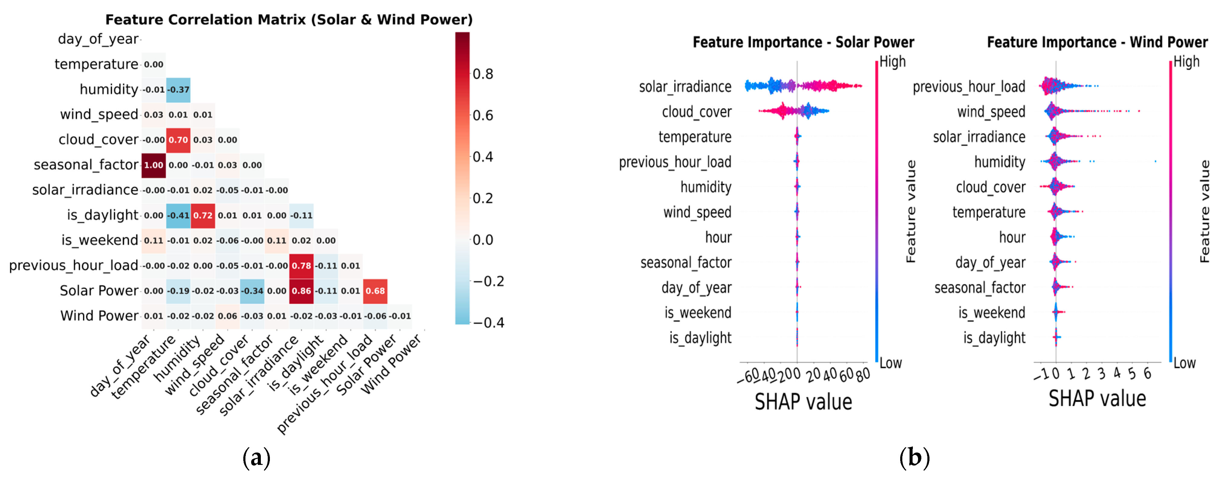
As depicted in Figure 6a, the heatmap shows that solar irradiance and solar power are strongly positively correlated, as are wind speed and wind power. This confirms that these two factors have the most effect on renewable generation. Cloud cover harms solar output, while sunshine and seasonal conditions have a mild effect. These findings confirm the significance of environmental factors in modeling renewable variability. The analysis supports the use of strong feature selection to enhance the proposed energy forecasting framework’s ability to make accurate predictions. Figure 6b presents the SHAP-based feature importance obtained for solar and wind power forecasting. The SHAP analysis quantifies the contribution of each meteorological, temporal, and historical feature to the prediction output, with solar irradiance, cloud cover, wind speed, seasonal factor, and previous-hour load exhibiting comparatively higher contributions. The mean absolute SHAP contribution of the $j$-th feature is calculated over the training samples as $\overline{\mid {\varphi }_j\mid }$, and the corresponding adaptive feature weight is normalized according to $w_j=\overline{\mid {\varphi }_j\mid }/{\sum }_{k=1}^F\overline{\mid {\varphi }_k\mid }$, where $F$ denotes the number of input features and ${\varphi }_j$ represents the SHAP contribution of feature $j$. The weighted input representation is subsequently obtained as ${\tilde{x}}_{t,j}=w_j{x}_{t,j}$, where $x_{t,j}$ denotes the original value of feature $j$ at time $t$. The resulting weighted feature representation is supplied to the BiLSTM–TFT prediction module, enabling features with greater predictive contribution to exert a proportionally stronger influence on the forecasting representation. The SHAP-derived weights are generated from the training data and applied consistently during model inference, while SHAP weighting is not introduced as an additional term in the forecasting loss function. This procedure establishes a direct computational link between feature contribution analysis and adaptive input weighting, thereby improving the transparency and reproducibility of the forecasting stage.

The dynamic feature-weighting mechanism combines the VSN’s learned variable-selection capability with SHAP-based prediction contributions. For an input feature vector $X\left(t\right)=\left\{x_1,\left(t\right),x_2,\left(t\right)\dots x_F\left(t\right)\right\}$, the SHAP contribution of feature $j$ at time $t$ is denoted by ${\varphi }_j\left(t\right)$. The normalized SHAP relevance is calculated as $s_j\left(t\right)={\displaystyle \frac{\mid {\varphi }_j\left(t\right)\mid }{{\displaystyle {\sum }_{k=1}^F}\mid {\varphi }_k\left(t\right)\mid }}.$ The VSN generates a feature-selection score through the SoftMax operation, $v_j\left(t\right)={\displaystyle \frac{\mathrm{e}\mathrm{x}\mathrm{p}\left(z_j\left(t\right)\right)}{{\displaystyle {\sum }_{k=1}^F}\mathrm{e}\mathrm{x}\mathrm{p}\left(z_k\left(t\right)\right)}},$ where $z_j\left(t\right)$ denotes the VSN selection logit for feature $j$. The final dynamic variable weight is obtained by combining these two relevance measures: $w_{\mathrm{v}\mathrm{a}\mathrm{r},j}\left(t\right)={\displaystyle \frac{v_j\left(t\right)s_j\left(t\right)}{{\displaystyle {\sum }_{k=1}^F}{v}_k\left(t\right)s_k\left(t\right)}}.$ The corresponding weighted feature is then expressed as ${\tilde{x}}_j\left(t\right)=w_{\mathrm{v}\mathrm{a}\mathrm{r},j}\left(t\right)x_j\left(t\right).$ The resulting weighted representation $\tilde{X}\left(t\right)$ is provided to the BiLSTM–TFT forecasting module. This formulation enables the VSN to learn feature-selection scores while SHAP values introduce prediction-specific feature relevance into the final variable weighting. Consequently, $w_{\mathrm{v}\mathrm{a}\mathrm{r}}\left(t\right)$ varies according to the relative contribution of the input variables to the forecasting output, providing an explicit mechanism for adaptive feature prioritization.

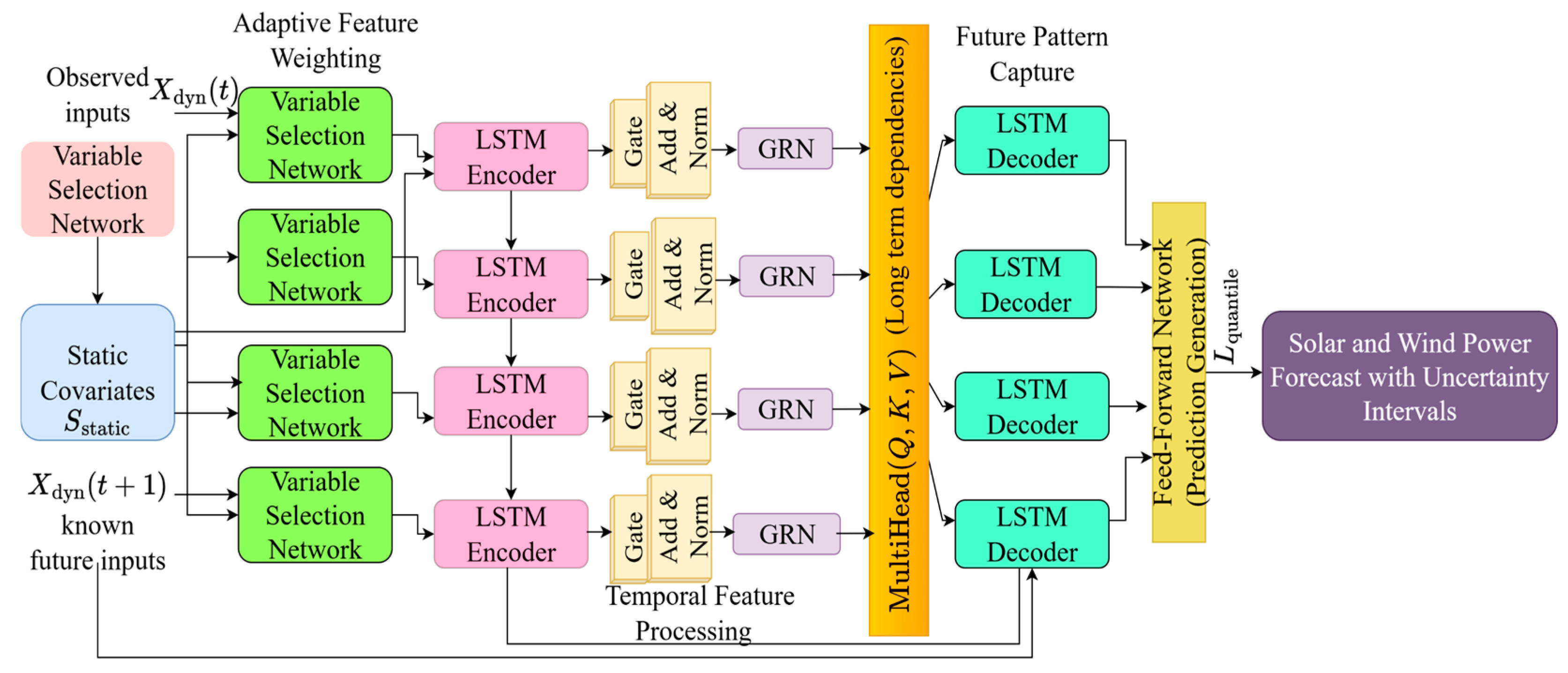
To optimize the model, a variable selection network, as shown in Figure 7, is used to determine the importance of each input feature. Observed inputs, static covariates, and known future inputs are processed through variable selection networks to weight important features adaptively.

The selection weights ${\mathrm{w}}_{\mathrm{v}\mathrm{a}\mathrm{r}}$ are calculated for each time step and variable to dynamically control their contribution. The feature vectors ${\mathrm{X}}_{\mathrm{t}}$ are transformed using the GRN, and variable selection weights ${\mathrm{w}}_{\mathrm{t}}$ are computed as in Equations (10) and (11),

$${\widehat{\mathrm{X}}}_{\mathrm{v}\mathrm{a}\mathrm{r}}\left(\mathrm{t}\right)=\mathrm{G}\mathrm{R}\mathrm{N}\left({\mathrm{X}}_{\mathrm{v}\mathrm{a}\mathrm{r}}\left(\mathrm{t}\right),{\mathrm{S}}_{\mathrm{s}\mathrm{t}\mathrm{a}\mathrm{t}\mathrm{i}\mathrm{c}}\right)$$

(10)

$${\mathrm{w}}_{\mathrm{v}\mathrm{a}\mathrm{r}}\left(\mathrm{t}\right)=\mathsf{\sigma }\left({\mathrm{W}}_{\mathrm{v}\mathrm{s}\mathrm{n}}·\left[{\mathrm{h}}_{\mathrm{t}-1},{\widehat{\mathrm{X}}}_{\mathrm{v}\mathrm{a}\mathrm{r}}\left(\mathrm{t}\right)\right]+{\mathrm{b}}_{\mathrm{v}\mathrm{s}\mathrm{n}}\right)$$

(11)

where ${\widehat{\mathrm{X}}}_{\mathrm{v}\mathrm{a}\mathrm{r}}\left(\mathrm{t}\right)$ is the transformed feature vector at time $\mathrm{t}$, produced by GRN, and the variable selection weight that determines the importance of the features ${\mathrm{w}}_{\mathrm{v}\mathrm{a}\mathrm{r}}\left(\mathrm{t}\right)$. $\mathsf{\sigma }$ is the sigmoid function that squashes the selection weight values between 0 and 1. The terms ${\mathrm{W}}_{\mathrm{v}\mathrm{s}\mathrm{n}}$ and ${\mathrm{b}}_{\mathrm{v}\mathrm{s}\mathrm{n}}$ are the weights and biases of the variable selection network. The output of the selection network ${\widehat{\mathrm{X}}}_{\mathrm{v}\mathrm{a}\mathrm{r}}\left(\mathrm{t}\right)$ is then weighted by the selection weights ${\mathrm{w}}_{\mathrm{v}\mathrm{a}\mathrm{r}}\left(\mathrm{t}\right)$ ensuring that only the relevant features are passed forward in the network. The temporal fusion layer combines the transformed features and applies multi-head attention to capture long-term dependencies in time-series data. Let ${\mathrm{h}}_{\mathrm{e}\mathrm{n}\mathrm{c}}\left(\mathrm{t}\right)$ be the encoded feature vector at time $\mathrm{t}$, after passing through the temporal processing layers. The self-attention mechanism is applied to both encoded and decoded features. The self-attention mechanism is computed as given in Equation (12).

$$\mathrm{A}\mathrm{t}\mathrm{t}\mathrm{e}\mathrm{n}\mathrm{t}\mathrm{i}\mathrm{o}\mathrm{n}\left(\mathrm{Q},\mathrm{K},\mathrm{V}\right)=\mathrm{s}\mathrm{o}\mathrm{f}\mathrm{t}\mathrm{m}\mathrm{a}\mathrm{x}\left({\displaystyle \frac{\mathrm{Q}{\mathrm{K}}^{\mathrm{T}}}{\sqrt{{\mathrm{d}}_{\mathrm{k}}}}}\right)\mathrm{V}$$

(12)

where $\mathrm{Q}$ is the query vector, representing the current time step’s processed feature vector, and $\mathrm{K}$ is the key vector, representing past feature vectors that provide context to the current step. The value vector $\mathrm{V}$ contains the data that will be weighted and used in the attention mechanism, and ${\mathrm{d}}_{\mathrm{k}}$ is the dimension of the key vectors. The multi-head attention is applied to the temporal feature vectors ${\mathrm{X}}_{\mathrm{d}\mathrm{y}\mathrm{n}}\left(\mathrm{t}\right)$ across multiple attention heads derived in Equation (13).

$$\mathrm{M}\mathrm{u}\mathrm{l}\mathrm{t}\mathrm{i}\mathrm{H}\mathrm{e}\mathrm{a}\mathrm{d}\left(\mathrm{Q},\mathrm{K},\mathrm{V}\right)=\mathrm{C}\mathrm{o}\mathrm{n}\mathrm{c}\mathrm{a}\mathrm{t}\left({\mathrm{h}\mathrm{e}\mathrm{a}\mathrm{d}}_1,{\mathrm{h}\mathrm{e}\mathrm{a}\mathrm{d}}_2,\dots ,{\mathrm{h}\mathrm{e}\mathrm{a}\mathrm{d}}_{\mathrm{h}}\right){\mathrm{W}}^{\mathrm{O}}$$

(13)

where $\mathrm{h}$ is the number of attention heads, and ${\mathrm{W}}^{\mathrm{O}}$ is the output weight matrix used to combine the outputs from all heads. The final representation from the MHA is then passed through a feed-forward network to generate predictions for the future time steps. The loss function used for training the TFT model is the quantile loss, which is particularly useful in time-series forecasting where the uncertainty of predictions needs to be accounted for. The quantile loss function ${\mathcal{L}}_{\mathrm{q}\mathrm{u}\mathrm{a}\mathrm{n}\mathrm{t}\mathrm{i}\mathrm{l}\mathrm{e}}$ is defined as

$${\mathcal{L}}_{\mathrm{q}\mathrm{u}\mathrm{a}\mathrm{n}\mathrm{t}\mathrm{i}\mathrm{l}\mathrm{e}}={\displaystyle \frac{1}{\mathrm{N}}}{\displaystyle {\sum }_{\mathrm{i}=1}^{\mathrm{N}}}\left({\widehat{\mathrm{y}}}_{\mathrm{i}}-{\mathrm{y}}_{\mathrm{i}}\right)·\left(\mathsf{\tau }-1\left({\mathrm{y}}_{\mathrm{i}}\ge {\widehat{\mathrm{y}}}_{\mathrm{i}}\right)\right)$$

(14)

In Equation (14), the predicted energy generation is termed ${\widehat{\mathrm{y}}}_{\mathrm{i}}$ for wind power or solar power at time $\mathrm{i}$, with $\mathrm{N}$ as the number of samples in the batch. The term ${\mathrm{y}}_{\mathrm{i}}$ acts as actual energy generation at time $\mathrm{i}$, where $\mathsf{\tau }\in \left\{\mathrm{0.1,0.5,0.9}\right\}$ represents the different quantile values, with one as an indicator function, checking whether the exact value is greater or less than the predicted value. This function effectively minimizes the forecasting error across different quantiles, modeling uncertainty in renewable energy predictions. It enables the model to predict a range of possible future values, which is useful for quantifying uncertainty in forecasting future renewable generation. The workflow of the proposed Algorithm 1 I is provided as:

Algorithm 1: IBT-PPO workflow.

Input: Weather data $W$, historical data $H$, grid data $G$ Output: Energy Dispatch Decisions $D$ 1: # Preprocessing 2: $X_{dyn}\leftarrow Normalize\left(\left[W,H,G\right]\right)$ 3: $S_{static}\leftarrow \left[latitude,longitude,{Site}_{info}\right]$ 4: # BiLSTM temporal representation 5: $H_{fwd}\leftarrow {BiLSTM}_{forward}\left(X_{dyn}\right)$ 6: $H_{bwd}\leftarrow {BiLSTM}_{backward}\left(reverse\left(X_{dyn}\right)\right)$ 7: $H_{Bi-LSTM}\leftarrow Concat\left(H_{fwd},H_{bwd}\right)$ 8: # Causal forecasting loop 9: for $t=1$ to $T-1$ do 10: ${\widehat{P}}_{wind,t+1},{\widehat{P}}_{solar,t+1}\leftarrow TFT\left(X_{dyn},\left[1:t\right]S_{static}\right)$ 11: end for 12: # Construct states and act with PPO 13: for $t=1$ to $T$ do 14: $s_t=\left[b_t,g_t,{\widehat{P}}_{wind,t},{\widehat{P}}_{solar,t},loa{d}_{demand,t}\right]$ 15: $a_t={\pi }_{\theta }\left(s_t\right)$ 16: $R_t\leftarrow -cost\left(a_t,s_t\right)+\alpha \hspace{0.17em}renewabl{e}_{util}\left(a_t\right)-\beta \hspace{0.17em}constrain{t}_{violation}\left(a_t\right)$ 17: $s_{t+1}\leftarrow Environment\_step\left(s_t,a_t\right)$ 18: end for 19: # PPO update 20: ${\pi }_{new},V_{new}\leftarrow PPO\_update\left(\left\{s_t\right\},\left\{a_t\right\},\left\{R_t\right\},{\pi }_{old}\right)$ 21: # Final dispatch decision generation 22: for $t=1$ to $horizon$ do 23: if ${\widehat{P}}_{renewable}\left(t\right)>loa{d}_{demand}\left(t\right)$ then 24: if $batter{y}_{level}<ma{x}_{capacity}$ then 25: $D\left[t\right]\leftarrow charg{e}_{battery}\left(exces{s}_{power}\right)$ 26: else 27: $D\left[t\right]\leftarrow sel{l}_{to\_grid}\left(exces{s}_{power}\right)$ 28: end if 29: else 30: $deficit\leftarrow loa{d}_{demand}\left(t\right)-{\widehat{P}}_{renewable}\left(t\right)$ 31: if $batter{y}_{level}>mi{n}_{capacity}$ then 32: $discharged\leftarrow min\left(d,eficitavailabl{e}_{battery}\right)$ 33: $D\left[t\right]\leftarrow discharg{e}_{battery}\left(discharged\right)$ 34: $remainin{g}_{deficit}\leftarrow deficit-discharged$ 35: if $remainin{g}_{deficit}>0$ then 36: $D\left[t\right]\leftarrow D\left[t\right]+bu{y}_{from\_grid}\left(remainin{g}_{deficit}\right)$ 37: end if 38: else 39: $D\left[t\right]\leftarrow bu{y}_{from\_grid}\left(deficit\right)$ 40: end if 41: end if 42: end for 43: return

3.4. Stage 2: PPO for Energy Planning

Once wind and solar power generation has been predicted, the next step is to optimize energy scheduling. This is done using PPO, an RL algorithm that is used to decide how to dispatch renewable energy, charge/discharge the battery, and rely on the grid. The state, action, and reward functions are calculated as follows.

The state space ${\mathrm{s}}_{\mathrm{t}}$ consists of the following features: ${\mathrm{b}}_{\mathrm{t}}$ represents the current energy stored in the battery at time $\mathrm{t}$. The grid power consumption ${\mathrm{g}}_{\mathrm{t}}$ indicates the amount of energy being drawn from the grid at time $\mathrm{t}$. The renewable power generation ${\mathrm{P}}_{\mathrm{w}\mathrm{i}\mathrm{n}\mathrm{d},\mathrm{t}}$ and ${\mathrm{P}}_{\mathrm{s}\mathrm{o}\mathrm{l}\mathrm{a}\mathrm{r},\mathrm{t}}$ are generated by wind and solar energy at time $\mathrm{t}$. Thus, the state vector at time $\mathrm{t}$ is given as ${\mathrm{s}}_{\mathrm{t}}=\left[{\mathrm{b}}_{\mathrm{t}},{\mathrm{g}}_{\mathrm{t}},{\mathrm{P}}_{\mathrm{w}\mathrm{i}\mathrm{n}\mathrm{d},\mathrm{t}},{\mathrm{P}}_{\mathrm{s}\mathrm{o}\mathrm{l}\mathrm{a}\mathrm{r},\mathrm{t}},{\mathrm{l}\mathrm{o}\mathrm{a}\mathrm{d}}_{\mathrm{d}\mathrm{e}\mathrm{m}\mathrm{a}\mathrm{n}\mathrm{d},\mathrm{t}}\right]$ with the action space ${\mathrm{a}}_{\mathrm{t}}={\mathsf{\pi }}_{\mathsf{\theta }}\left({\mathrm{s}}_{\mathrm{t}}\right)$ including the decision to discharge the battery, charge the battery, and dispatch renewable energy, in addition to including grid power when renewable power is insufficient. The heterogeneous reward components are normalized before their incorporation into the PPO reward function to ensure comparable numerical contributions during policy optimization. The operational cost $C_{\mathrm{o}\mathrm{p}\mathrm{e}\mathrm{r}\mathrm{a}\mathrm{t}\mathrm{i}\mathrm{o}\mathrm{n}\mathrm{a}\mathrm{l}}$, renewable power $P_{\mathrm{r}\mathrm{e}\mathrm{n}\mathrm{e}\mathrm{w}\mathrm{a}\mathrm{b}\mathrm{l}\mathrm{e}}$, and grid power $P_{\mathrm{g}\mathrm{r}\mathrm{i}\mathrm{d}}$ are independently scaled using min–max normalization based on the corresponding ranges obtained from the training data. For each component $X_t$, the normalized quantity is calculated as ${\widehat{X}}_t={\displaystyle \frac{X_t-X_{\mathrm{m}\mathrm{i}\mathrm{n}}}{X_{\mathrm{m}\mathrm{a}\mathrm{x}}-X_{\mathrm{m}\mathrm{i}\mathrm{n}}+ϵ}},$ where $X_{\mathrm{m}\mathrm{i}\mathrm{n}}$ and $X_{\mathrm{m}\mathrm{a}\mathrm{x}}$ denote the minimum and maximum training set values and $ϵ$ is a small positive constant. The normalized quantities ${\widehat{C}}_{\mathrm{o}\mathrm{p}\mathrm{e}\mathrm{r}\mathrm{a}\mathrm{t}\mathrm{i}\mathrm{o}\mathrm{n}\mathrm{a}\mathrm{l}}$, ${\widehat{P}}_{\mathrm{r}\mathrm{e}\mathrm{n}\mathrm{e}\mathrm{w}\mathrm{a}\mathrm{b}\mathrm{l}\mathrm{e}}$, and ${\widehat{P}}_{\mathrm{g}\mathrm{r}\mathrm{i}\mathrm{d}}$ are then incorporated into the reward function. This scaling converts the heterogeneous cost and power quantities into dimensionless values within a comparable numerical range, preventing a high-magnitude term from dominating the PPO objective and supporting stable policy, and value-function updates.

The reward function is designed to maximize renewable energy use while minimizing operational costs, subject to constraints on battery storage.

$${\mathrm{R}}_{\mathrm{t}}=\left\{\begin{array}{c}-{\mathrm{C}}_{\mathrm{o}\mathrm{p}\mathrm{e}\mathrm{r}\mathrm{a}\mathrm{t}\mathrm{i}\mathrm{o}\mathrm{n}\mathrm{a}\mathrm{l}}+{\mathsf{\lambda }}_{\mathrm{r}\mathrm{e}\mathrm{n}\mathrm{e}\mathrm{w}\mathrm{a}\mathrm{b}\mathrm{l}\mathrm{e}}·{\mathrm{P}}_{\mathrm{r}\mathrm{e}\mathrm{n}\mathrm{e}\mathrm{w}\mathrm{a}\mathrm{b}\mathrm{l}\mathrm{e}}-\mathsf{\gamma }·{\mathrm{P}}_{\mathrm{g}\mathrm{r}\mathrm{i}\mathrm{d}}+\mathsf{\rho }·1_{\mathrm{b}\mathrm{a}\mathrm{t}\mathrm{t}\mathrm{e}\mathrm{r}\mathrm{y}}\left({\mathrm{b}}_{\mathrm{t}}\right)+\\ \mathsf{\zeta }·\left({\displaystyle {\sum }_{\mathrm{t}=1}^{\mathrm{T}}}\left|{\mathrm{P}}_{\mathrm{g}\mathrm{r}\mathrm{i}\mathrm{d}}\left(\mathrm{t}\right)-{\mathrm{P}}_{\mathrm{r}\mathrm{e}\mathrm{n}\mathrm{e}\mathrm{w}\mathrm{a}\mathrm{b}\mathrm{l}\mathrm{e}}\left(\mathrm{T}\right)\right|\right)\\ {\mathrm{C}}_{\mathrm{o}\mathrm{p}\mathrm{e}\mathrm{r}\mathrm{a}\mathrm{t}\mathrm{i}\mathrm{o}\mathrm{n}\mathrm{a}\mathrm{l}}={\displaystyle {\sum }_{\mathrm{t}=1}^{\mathrm{T}}}{\mathrm{P}}_{\mathrm{g}\mathrm{r}\mathrm{i}\mathrm{d}}\left(\mathrm{t}\right)·{\mathrm{C}}_{\mathrm{g}\mathrm{r}\mathrm{i}\mathrm{d}}\left(\mathrm{t}\right) \mathrm{and} {\mathrm{C}}_{\mathrm{g}\mathrm{r}\mathrm{i}\mathrm{d}}\left(\mathrm{t}\right)=\left({\displaystyle \frac{{\mathrm{P}}_{\mathrm{g}\mathrm{r}\mathrm{i}\mathrm{d}}\left(\mathrm{t}\right)·{\mathrm{C}\mathrm{o}\mathrm{s}\mathrm{t}}_{\mathrm{g}\mathrm{r}\mathrm{i}\mathrm{d}}\left(\mathrm{t}\right)}{{\mathrm{P}}_{\mathrm{m}\mathrm{a}\mathrm{x}}}}\right)\\ {\mathrm{P}}_{\mathrm{r}\mathrm{e}\mathrm{n}\mathrm{e}\mathrm{w}\mathrm{a}\mathrm{b}\mathrm{l}\mathrm{e}}={\displaystyle {\sum }_{\mathrm{t}=1}^{\mathrm{T}}}\left({\mathsf{\eta }}_{\mathrm{s}\mathrm{o}\mathrm{l}\mathrm{a}\mathrm{r}}\left(\mathrm{t}\right)·{\mathrm{P}}_{\mathrm{s}\mathrm{o}\mathrm{l}\mathrm{a}\mathrm{r}}\left(\mathrm{t}\right)+{\mathsf{\eta }}_{\mathrm{w}\mathrm{i}\mathrm{n}\mathrm{d}}\left(\mathrm{t}\right)·{\mathrm{P}}_{\mathrm{w}\mathrm{i}\mathrm{n}\mathrm{d}}\left(\mathrm{t}\right)\right)\\ {\mathrm{P}}_{\mathrm{g}\mathrm{r}\mathrm{i}\mathrm{d}}={\displaystyle {\sum }_{\mathrm{t}=1}^{\mathrm{T}}}{\mathrm{P}}_{\mathrm{g}\mathrm{r}\mathrm{i}\mathrm{d}}\left(\mathrm{t}\right)\\ 1_{\mathrm{b}\mathrm{a}\mathrm{t}\mathrm{t}\mathrm{e}\mathrm{r}\mathrm{y}}\left({\mathrm{b}}_{\mathrm{t}}\right)=\left\{\begin{array}{c}1 \mathrm{if} {\mathrm{b}}_{\mathrm{t}}>\mathrm{threshold}\\ 0 \mathrm{otherwise}\end{array}\right.\end{array}\right.$$

(15)

where ${\mathrm{C}}_{\mathrm{o}\mathrm{p}\mathrm{e}\mathrm{r}\mathrm{a}\mathrm{t}\mathrm{i}\mathrm{o}\mathrm{n}\mathrm{a}\mathrm{l}}$ in Equation (15) is the cost of operations, ${\mathrm{P}}_{\mathrm{r}\mathrm{e}\mathrm{n}\mathrm{e}\mathrm{w}\mathrm{a}\mathrm{b}\mathrm{l}\mathrm{e}}$ is the dispatched renewable energy, and ${\mathrm{P}}_{\mathrm{g}\mathrm{r}\mathrm{i}\mathrm{d}}$ is the energy consumed from the grid, with the constraint ${\mathrm{b}}_{\mathrm{m}\mathrm{i}\mathrm{n}}\le {\mathrm{b}}_{\mathrm{t}}\le {\mathrm{b}}_{\mathrm{m}\mathrm{a}\mathrm{x}}$. The policy update for PPO is given by the following objective function, ensuring stability during updates. The policy function defines the probability of taking a specific action ${\mathrm{a}}_{\mathrm{t}}$ at time $\mathrm{t}$ based on the current state ${\mathrm{s}}_{\mathrm{t}}$, followed by comfort penalty $\mathsf{\zeta }·\left({\displaystyle {\sum }_{\mathrm{t}=1}^{\mathrm{T}}}\left|{\mathrm{P}}_{\mathrm{g}\mathrm{r}\mathrm{i}\mathrm{d}}\left(\mathrm{t}\right)-{\mathrm{P}}_{\mathrm{r}\mathrm{e}\mathrm{n}\mathrm{e}\mathrm{w}\mathrm{a}\mathrm{b}\mathrm{l}\mathrm{e}}\left(\mathrm{T}\right)\right|\right)$ to encourage energy consumption from renewable sources, minimizing reliance on grid power. This stochastic policy enables PPO to explore various energy dispatch strategies, such as charging and discharging the battery and renewable dispatch, which is essential for optimizing energy use in hybrid renewable energy systems (Equation (16)).

$${\mathsf{\pi }}_{\mathsf{\theta }}\left({\mathrm{a}}_{\mathrm{t}}|{\mathrm{s}}_{\mathrm{t}}\right)=\mathrm{s}\mathrm{o}\mathrm{f}\mathrm{t}\mathrm{m}\mathrm{a}\mathrm{x}\left({\mathrm{W}}_{\mathsf{\pi }}·\mathrm{R}\mathrm{e}\mathrm{L}\mathrm{U}\left({\mathrm{W}}_{\mathrm{h}}·{\mathrm{s}}_{\mathrm{t}}+{\mathrm{b}}_{\mathrm{h}}\right)+{\mathrm{b}}_{\mathsf{\pi }}\right)$$

(16)

The term ${\mathsf{\pi }}_{\mathsf{\theta }}\left({\mathrm{a}}_{\mathrm{t}}|{\mathrm{s}}_{\mathrm{t}}\right)$ is the current policy, in which ${\mathrm{W}}_{\mathsf{\pi }}\in {\mathbb{R}}^{{\mathrm{n}}_{\mathrm{a}}\times {\mathrm{n}}_{\mathrm{h}}}$ acts as the weight matrix for the policy function and ${\mathrm{W}}_{\mathrm{h}}\in {\mathbb{R}}^{{\mathrm{n}}_{\mathrm{h}}\times {\mathrm{n}}_{\mathrm{s}}}$ as the hidden layer weights, with the bias terms. The term ${\mathrm{A}}_{\mathrm{t}}$ is the advantage function with the policy update performed as ${\mathsf{\theta }}_{\mathrm{n}\mathrm{e}\mathrm{w}}={\mathsf{\theta }}_{\mathrm{o}\mathrm{l}\mathrm{d}}+\mathsf{\alpha }{\nabla }_{\mathsf{\theta }}\mathrm{J}\left(\mathsf{\theta }\right)$.

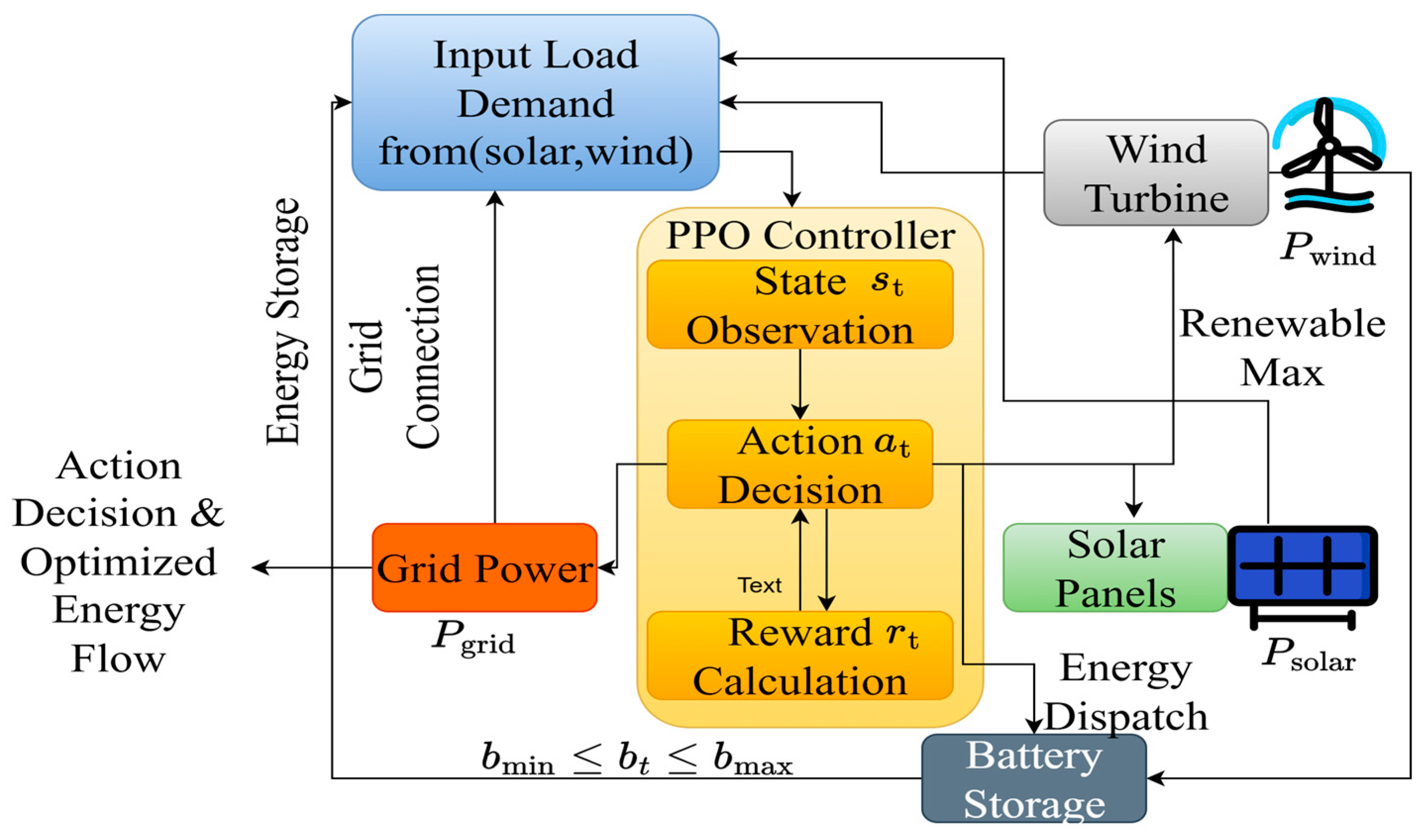
As illustrated in Figure 8, the PPO controller value function estimates the expected reward for a given state ${\mathrm{s}}_{\mathrm{t}}$ helping the PPO model to evaluate the quality of the current state and guide action decisions in the optimization process. The observed inputs include load demand, renewable generation from wind and solar sources, and battery charge levels. These inputs from the state observations guide the PPO controller’s action decisions for energy dispatch. It enables PPO to calculate the advantage function, which helps the agent learn better policies by considering the difference between expected rewards and actual rewards. This value function is used in the PPO module to estimate state values and improve decision-making for energy scheduling. The PPO objective function is written as in Equations (17) and (18),

$$\mathrm{J}\left(\mathsf{\theta }\right)={\mathbb{E}}_{\mathrm{t}}\left[\mathrm{m}\mathrm{i}\mathrm{n}\left({\displaystyle \frac{{\mathsf{\pi }}_{\mathsf{\theta }}\left({\mathrm{a}}_{\mathrm{t}}|{\mathrm{s}}_{\mathrm{t}}\right)}{{\mathsf{\pi }}_{{\mathsf{\theta }}_{\mathrm{o}\mathrm{l}\mathrm{d}}}\left({\mathrm{a}}_{\mathrm{t}}|{\mathrm{s}}_{\mathrm{t}}\right)}}\right){\mathrm{A}}_{\mathrm{t}},\mathrm{c}\mathrm{l}\mathrm{i}\mathrm{p}\left({\displaystyle \frac{{\mathsf{\pi }}_{\mathsf{\theta }}\left({\mathrm{a}}_{\mathrm{t}}|{\mathrm{s}}_{\mathrm{t}}\right)}{{\mathsf{\pi }}_{{\mathsf{\theta }}_{\mathrm{o}\mathrm{l}\mathrm{d}}}\left({\mathrm{a}}_{\mathrm{t}}|{\mathrm{s}}_{\mathrm{t}}\right)}},1-\mathsf{ϵ},1+\mathsf{ϵ}\right){\mathrm{A}}_{\mathrm{t}}\right]$$

(17)

$$\begin{gathered} {\nabla }_{\mathsf{\theta }}{\mathrm{C}}_{\mathrm{t}\mathrm{o}\mathrm{t}\mathrm{a}\mathrm{l}}\left(\mathrm{t}\right)=\left({\displaystyle \frac{\partial {\mathrm{C}}_{\mathrm{r}\mathrm{e}\mathrm{n}\mathrm{e}\mathrm{w}\mathrm{a}\mathrm{b}\mathrm{l}\mathrm{e}}\left(\mathrm{t}\right)}{\partial {\mathrm{P}}_{\mathrm{w}\mathrm{i}\mathrm{n}\mathrm{d}}\left(\mathrm{t}\right)}}·{\nabla }_{\mathsf{\theta }}{\mathrm{P}}_{\mathrm{w}\mathrm{i}\mathrm{n}\mathrm{d}}\left(\mathrm{t}\right)+{\displaystyle \frac{\partial {\mathrm{C}}_{\mathrm{r}\mathrm{e}\mathrm{n}\mathrm{e}\mathrm{w}\mathrm{a}\mathrm{b}\mathrm{l}\mathrm{e}}\left(\mathrm{t}\right)}{\partial {\mathrm{P}}_{\mathrm{s}\mathrm{o}\mathrm{l}\mathrm{a}\mathrm{r}}\left(\mathrm{t}\right)}}·{\nabla }_{\mathsf{\theta }}{\mathrm{P}}_{\mathrm{s}\mathrm{o}\mathrm{l}\mathrm{a}\mathrm{r}}\left(\mathrm{t}\right)\right)+{\mathsf{\lambda }}_{\mathrm{g}\mathrm{r}\mathrm{i}\mathrm{d}}· \\ \left({\displaystyle \frac{\partial {\mathrm{C}}_{\mathrm{g}\mathrm{r}\mathrm{i}\mathrm{d}}\left(\mathrm{t}\right)}{\partial {\mathrm{P}}_{\mathrm{g}\mathrm{r}\mathrm{i}\mathrm{d}}\left(\mathrm{t}\right)}}·{\nabla }_{\mathsf{\theta }}{\mathrm{P}}_{\mathrm{g}\mathrm{r}\mathrm{i}\mathrm{d}}\left(\mathrm{t}\right)\right) \mathrm{w}\mathrm{h}\mathrm{e}\mathrm{r}\mathrm{e} {\mathsf{\theta }}_{\mathrm{t}+1}={\mathsf{\theta }}_{\mathrm{t}}+\mathsf{\alpha }·{\nabla }_{\mathsf{\theta }}{\mathrm{C}}_{\mathrm{t}\mathrm{o}\mathrm{t}\mathrm{a}\mathrm{l}}\left(\mathrm{t}\right) \end{gathered}$$

(18)

The total gradient of the cost function ${\nabla }_{\mathsf{\theta }}{\mathrm{C}}_{\mathrm{t}\mathrm{o}\mathrm{t}\mathrm{a}\mathrm{l}}\left(\mathrm{t}\right)$ at time $\mathrm{t}$ considers both renewable and grid costs. The partial derivative of the renewable cost with respect to wind power generation is ${\displaystyle \frac{\partial {\mathrm{C}}_{\mathrm{r}\mathrm{e}\mathrm{n}\mathrm{e}\mathrm{w}\mathrm{a}\mathrm{b}\mathrm{l}\mathrm{e}}\left(\mathrm{t}\right)}{\partial {\mathrm{P}}_{\mathrm{w}\mathrm{i}\mathrm{n}\mathrm{d}}\left(\mathrm{t}\right)}}$, and ${\nabla }_{\mathsf{\theta }}{\mathrm{P}}_{\mathrm{w}\mathrm{i}\mathrm{n}\mathrm{d}}\left(\mathrm{t}\right)$ is the gradient of wind power generation with respect to policy parameters $\mathsf{\theta }$. The partial derivative of the renewable cost with respect to solar power generation is ${\displaystyle \frac{\partial {\mathrm{C}}_{\mathrm{r}\mathrm{e}\mathrm{n}\mathrm{e}\mathrm{w}\mathrm{a}\mathrm{b}\mathrm{l}\mathrm{e}}\left(\mathrm{t}\right)}{\partial {\mathrm{P}}_{\mathrm{s}\mathrm{o}\mathrm{l}\mathrm{a}\mathrm{r}}\left(\mathrm{t}\right)}}$; ${\nabla }_{\mathsf{\theta }}{\mathrm{P}}_{\mathrm{s}\mathrm{o}\mathrm{l}\mathrm{a}\mathrm{r}}\left(\mathrm{t}\right)$ is the gradient of solar power generation with respect to policy parameters $\mathsf{\theta }$; and ${\mathsf{\lambda }}_{\mathrm{g}\mathrm{r}\mathrm{i}\mathrm{d}}$ is a grid cost penalty factor, balancing renewable energy usage with grid dependence. The partial derivative of the grid cost with respect to grid power generation is ${\displaystyle \frac{\partial {\mathrm{C}}_{\mathrm{g}\mathrm{r}\mathrm{i}\mathrm{d}}\left(\mathrm{t}\right)}{\partial {\mathrm{P}}_{\mathrm{g}\mathrm{r}\mathrm{i}\mathrm{d}}\left(\mathrm{t}\right)}}$; ${\nabla }_{\mathsf{\theta }}{\mathrm{P}}_{\mathrm{g}\mathrm{r}\mathrm{i}\mathrm{d}}\left(\mathrm{t}\right)$ acts as a gradient of grid power generation with respect to policy parameters $\mathsf{\theta }$; and the learning rate for policy updates is $\mathsf{\alpha }$ for a current policy ${\mathsf{\theta }}_{\mathrm{t}}$ at time $\mathrm{t}$, with the policy updated after applying the gradient-based optimization. With this use of a gradient policy, the agent controller process learns adaptively and optimizes the generation of renewable energy and grid power over time, improving efficiency and minimizing costs.

3.5. Uncertainty-Aware Planning

The PPO-generated schedules are subsequently adjusted according to the operator’s risk preference $\rho$ using lower, median, and upper predictive quantiles. The uncertainty-aware planning strategy accounts for the stochastic nature of renewable generation, particularly wind and solar power, which are sensitive to variations in weather and environmental conditions. Rather than relying on a single point forecast, the proposed framework uses probabilistic forecasts to represent the uncertainty range of renewable generation. For a risk-averse operator ($\rho <0.3$), the lower quantile $q_{0.1}$ is selected to obtain a conservative renewable-generation estimate. For a risk-seeking operator ($\rho >0.7$), the upper quantile $q_{0.9}$ is selected, whereas the median quantile $q_{0.5}$ is used for risk-neutral operation. The corresponding wind and solar allocations are defined in Equations (19) and (20).

$$P_{\mathrm{c}\mathrm{o}\mathrm{n}\mathrm{s}}^{\mathrm{w}\mathrm{i}\mathrm{n}\mathrm{d}}\left(t\right)=\left\{\begin{array}{cc}{q}_{0.1}^{\mathrm{w}\mathrm{i}\mathrm{n}\mathrm{d}}\left(t\right),& \rho <0.3\left(\text{risk-averse}\right),\\ q_{0.9}^{\mathrm{w}\mathrm{i}\mathrm{n}\mathrm{d}}\left(t\right),& \rho >0.7\left(\text{risk-seeking}\right),\\ q_{0.5}^{\mathrm{w}\mathrm{i}\mathrm{n}\mathrm{d}}\left(t\right),& 0.3\le \rho \le 0.7\left(\text{risk-neutral}\right).\end{array}\right.$$

(19)

$$P_{\mathrm{c}\mathrm{o}\mathrm{n}\mathrm{s}}^{\mathrm{s}\mathrm{o}\mathrm{l}\mathrm{a}\mathrm{r}}\left(t\right)=\left\{\begin{array}{cc}{q}_{0.1}^{\mathrm{s}\mathrm{o}\mathrm{l}\mathrm{a}\mathrm{r}}\left(t\right),& \rho <0.3\left(\text{risk-averse}\right),\\ q_{0.9}^{\mathrm{s}\mathrm{o}\mathrm{l}\mathrm{a}\mathrm{r}}\left(t\right),& \rho >0.7\left(\text{risk-seeking}\right),\\ q_{0.5}^{\mathrm{s}\mathrm{o}\mathrm{l}\mathrm{a}\mathrm{r}}\left(t\right),& 0.3\le \rho \le 0.7\left(\text{risk-neutral}\right).\end{array}\right.$$

(20)

The uncertainty ranges of wind and solar generation are calculated as

$$U_{\mathrm{w}\mathrm{i}\mathrm{n}\mathrm{d}}\left(t\right)=q_{0.9}^{\mathrm{w}\mathrm{i}\mathrm{n}\mathrm{d}}\left(t\right)-q_{0.1}^{\mathrm{w}\mathrm{i}\mathrm{n}\mathrm{d}}\left(t\right)$$

(21)

$$U_{\mathrm{s}\mathrm{o}\mathrm{l}\mathrm{a}\mathrm{r}}\left(t\right)=q_{0.9}^{\mathrm{s}\mathrm{o}\mathrm{l}\mathrm{a}\mathrm{r}}\left(t\right)-q_{0.1}^{\mathrm{s}\mathrm{o}\mathrm{l}\mathrm{a}\mathrm{r}}\left(t\right)$$

(22)

The required battery reserve is determined from the combined renewable-energy uncertainty while maintaining a minimum reserve of 10% of the total battery capacity:

$$b_{\mathrm{r}\mathrm{e}\mathrm{s}\mathrm{e}\mathrm{r}\mathrm{v}\mathrm{e}}\left(t\right)=\max \left[0.1,C_{\mathrm{t}\mathrm{o}\mathrm{t}\mathrm{a}\mathrm{l}}\left(U_{\mathrm{w}\mathrm{i}\mathrm{n}\mathrm{d}}\left(t\right)+U_{\mathrm{s}\mathrm{o}\mathrm{l}\mathrm{a}\mathrm{r}}\left(t\right)\right)\mathsf{\Delta }t\right]$$

(23)

where $C_{\mathrm{t}\mathrm{o}\mathrm{t}\mathrm{a}\mathrm{l}}$ denotes the nominal battery capacity and $\mathsf{\Delta }t$ represents the scheduling interval. The multiplication by $\mathsf{\Delta }t$ converts the renewable-power uncertainty from kW to energy in kWh, ensuring dimensional consistency with the battery capacity. The risk-adjusted dispatch is subsequently obtained as

$$D_{\mathrm{r}\mathrm{i}\mathrm{s}\mathrm{k}}\left(t\right)=\mathrm{optimize}\left(P_{\mathrm{c}\mathrm{o}\mathrm{n}\mathrm{s}}^{\mathrm{w}\mathrm{i}\mathrm{n}\mathrm{d}},\left(t\right),P_{\mathrm{c}\mathrm{o}\mathrm{n}\mathrm{s}}^{\mathrm{s}\mathrm{o}\mathrm{l}\mathrm{a}\mathrm{r}}\left(t\right)b_{\mathrm{r}\mathrm{e}\mathrm{s}\mathrm{e}\mathrm{r}\mathrm{v}\mathrm{e}}\left(t\right)\right)$$

(24)

This formulation enables the proposed scheduling strategy to adapt to different operator risk preferences while explicitly accounting for uncertainty in renewable-energy generation. The uncertainty-aware planning and energy schedule ensures that decisions align with the operator’s goals, whether that means reducing cost volatility, increasing the use of renewable energy, or finding the optimal balance between trade-offs. Adding a safety buffer that is proportional to both the system’s capacity and the uncertainty observed makes the system even more reliable against forecast errors. The uncertainty-aware module stabilizes energy scheduling by reducing the likelihood of extreme events, making hybrid renewable energy systems more stable overall, as defined in Algorithm 2.

Algorithm 2. Uncertainty-aware planning.

Input: Quantile predictions $\mathrm{Q}$, risk tolerance $\mathsf{\rho }$

Output: Risk-adjusted decisions ${\mathrm{D}}_{\mathrm{r}\mathrm{i}\mathrm{s}\mathrm{k}}$

1:  $\mathrm{f}\mathrm{o}\mathrm{r} \mathrm{t}= 1 \mathrm{t}\mathrm{o} \mathrm{T} \mathrm{d}\mathrm{o}$

2:    ${\mathrm{U}}_{\mathrm{w}\mathrm{i}\mathrm{n}\mathrm{d}}\left(\mathrm{t}\right)\leftarrow {\mathrm{q}}_{0.9}^{\mathrm{w}\mathrm{i}\mathrm{n}\mathrm{d}}\left(\mathrm{t}\right)-{\mathrm{q}}_{0.1}^{\mathrm{w}\mathrm{i}\mathrm{n}\mathrm{d}}\left(\mathrm{t}\right)$

3:    ${\mathrm{U}}_{\mathrm{s}\mathrm{o}\mathrm{l}\mathrm{a}\mathrm{r}}\left(\mathrm{t}\right)\leftarrow {\mathrm{q}}_{0.9}^{\mathrm{s}\mathrm{o}\mathrm{l}\mathrm{a}\mathrm{r}}\left(\mathrm{t}\right)-{\mathrm{q}}_{0.1}^{\mathrm{s}\mathrm{o}\mathrm{l}\mathrm{a}\mathrm{r}}\left(\mathrm{t}\right)$

4:    $\mathrm{i}\mathrm{f}\mathsf{\rho }<0.3 \mathrm{t}\mathrm{h}\mathrm{e}\mathrm{n}$            # risk-averse

5:      ${\mathrm{P}}_{\mathrm{c}\mathrm{o}\mathrm{n}\mathrm{s}}^{\mathrm{w}\mathrm{i}\mathrm{n}\mathrm{d}}\left(\mathrm{t}\right)\leftarrow {\mathrm{q}}_{0.1}^{\mathrm{w}\mathrm{i}\mathrm{n}\mathrm{d}}\left(\mathrm{t}\right)$

6:      ${\mathrm{P}}_{\mathrm{c}\mathrm{o}\mathrm{n}\mathrm{s}}^{\mathrm{s}\mathrm{o}\mathrm{l}\mathrm{a}\mathrm{r}}\left(\mathrm{t}\right)\leftarrow {\mathrm{q}}_{0.1}^{\mathrm{s}\mathrm{o}\mathrm{l}\mathrm{a}\mathrm{r}}\left(\mathrm{t}\right)$

7:    $\mathrm{e}\mathrm{l}\mathrm{s}\mathrm{e} \mathrm{i}\mathrm{f}\mathsf{\rho }>0.7 \mathrm{t}\mathrm{h}\mathrm{e}\mathrm{n}$          # risk-seeking

8:      ${\mathrm{P}}_{\mathrm{c}\mathrm{o}\mathrm{n}\mathrm{s}}^{\mathrm{w}\mathrm{i}\mathrm{n}\mathrm{d}}\left(\mathrm{t}\right)\leftarrow {\mathrm{q}}_{0.9}^{\mathrm{w}\mathrm{i}\mathrm{n}\mathrm{d}}\left(\mathrm{t}\right)$

9:      ${\mathrm{P}}_{\mathrm{c}\mathrm{o}\mathrm{n}\mathrm{s}}^{\mathrm{s}\mathrm{o}\mathrm{l}\mathrm{a}\mathrm{r}}\left(\mathrm{t}\right)\leftarrow {\mathrm{q}}_{0.9}^{\mathrm{s}\mathrm{o}\mathrm{l}\mathrm{a}\mathrm{r}}\left(\mathrm{t}\right)$

10:     else                # risk-neutral

11:       ${\mathrm{P}}_{\mathrm{c}\mathrm{o}\mathrm{n}\mathrm{s}}^{\mathrm{s}\mathrm{o}\mathrm{l}\mathrm{a}\mathrm{r}}\left(\mathrm{t}\right)\leftarrow {\mathrm{q}}_{0.5}^{\mathrm{s}\mathrm{o}\mathrm{l}\mathrm{a}\mathrm{r}}\left(\mathrm{t}\right)$

12:       ${\mathrm{P}}_{\mathrm{c}\mathrm{o}\mathrm{n}\mathrm{s}}^{\mathrm{s}\mathrm{o}\mathrm{l}\mathrm{a}\mathrm{r}}\left(\mathrm{t}\right)\leftarrow {\mathrm{q}}_{0.5}^{\mathrm{s}\mathrm{o}\mathrm{l}\mathrm{a}\mathrm{r}}\left(\mathrm{t}\right)$

13:     end if

14:     $\mathrm{s}\mathrm{a}\mathrm{f}\mathrm{e}\mathrm{t}\mathrm{y}\_\mathrm{b}\mathrm{u}\mathrm{f}\mathrm{f}\mathrm{e}\mathrm{r}\leftarrow \mathrm{m}\mathrm{a}\mathrm{x}(0.1\ast \mathrm{t}\mathrm{o}\mathrm{t}\mathrm{a}\mathrm{l}\_\mathrm{c}\mathrm{a}\mathrm{p}\mathrm{a}\mathrm{c}\mathrm{i}\mathrm{t}\mathrm{y},{\mathrm{U}}_{\mathrm{w}\mathrm{i}\mathrm{n}\mathrm{d}}+{\mathrm{U}}_{\mathrm{s}\mathrm{o}\mathrm{l}\mathrm{a}\mathrm{r}})$

15:     ${\mathrm{D}}_{\mathrm{r}\mathrm{i}\mathrm{s}\mathrm{k}}\left(\mathrm{t}\right)=\mathrm{o}\mathrm{p}\mathrm{t}\mathrm{i}\mathrm{m}\mathrm{i}\mathrm{z}\mathrm{e}\left({\mathrm{P}}_{\mathrm{c}\mathrm{o}\mathrm{n}\mathrm{s}}^{\mathrm{w}\mathrm{i}\mathrm{n}\mathrm{d}}\left(\mathrm{t}\right),{\mathrm{P}}_{\mathrm{c}\mathrm{o}\mathrm{n}\mathrm{s}}^{\mathrm{s}\mathrm{o}\mathrm{l}\mathrm{a}\mathrm{r}}\left(\mathrm{t}\right),\mathrm{b}\left(\mathrm{t}\right)\right)$

16: $\mathrm{e}\mathrm{n}\mathrm{d} \mathrm{f}\mathrm{o}\mathrm{r}$

17: return ${\mathrm{D}}_{\mathrm{r}\mathrm{i}\mathrm{s}\mathrm{k}}$

The calibration and reliability of the probabilistic forecasts are evaluated by comparing the observed renewable-generation values with the predicted quantile intervals across the forecasting horizons. The Prediction Interval Coverage Probability (PICP) is used to measure the proportion of observations contained within the predicted interval, while the Mean Prediction Interval Width (MPIW) quantifies the sharpness of the interval. The Winkler score is additionally used to jointly assess interval coverage and width, thereby penalizing intervals that are excessively wide or fail to contain the observed value. Calibration is assessed by comparing the empirical coverage with the corresponding nominal confidence levels, such as 80%, 90%, and 95%.

In conclusion, the IBT-PPO workflow improves hybrid renewable energy system energy management through advanced forecasting and efficient planning. Stage 1 uses a Bi-LSTM with TFT to reliably predict short-term wind, solar, and energy demand trends. Bi-LSTM collects temporal dependencies from past and future data, while TFT refines predictions via adaptive feature selection, MHA, and gating techniques to handle uncertainty. After stage 2, the PPO algorithm optimizes battery charging, grid consumption, and energy dispatch by maximizing renewable energy use and minimizing expenses using projections. Through iterative learning, the system uses uncertainty-aware planning and probabilistic forecasts and risk tolerance to modify. So, the research ensures scalable, reliable, and adaptive renewable energy planning. The PPO training process converges after approximately 720 episodes, with the mean episodic reward improving from −148.6 to −76.9, while the actor loss decreases from 0.184 to 0.021 and the critic loss decreases from 0.426 to 0.038. Sensitivity analysis of the reward coefficients is performed by varying $\alpha$, $\beta$, and $\gamma$ while maintaining $\alpha +\beta +\gamma =1$. Among the evaluated configurations, $\alpha =0.35$, $\beta =0.40$, and $\gamma =0.25$ produce the most balanced scheduling performance, achieving an operating cost of 76.9, renewable-energy utilization of 95.5%, renewable-energy curtailment of 2.7%, and one constraint violation. The convergence behavior and reward-weight analysis demonstrate stable PPO policy learning and quantify the sensitivity of scheduling performance to the relative weighting of economic cost, renewable-energy utilization, and operational constraints, providing a reproducible basis for the adopted reinforcement learning configuration.

4. Simulation and Experimental Setup

The research idea is implemented in Python using TensorFlow (v2.16.1), PyTorch (v2.3.1), NumPy (v1.26.4), and Pandas (v2.2.2) to work with hybridized renewable energy data. The experiment uses an Intel i7 processor with 16 GB of RAM and an NVIDIA RTX 3060 GPU for parallel processing. The data consists of hourly time-series data on various factors, including wind and solar power generation, weather conditions, and electricity usage.

The experiments use a fixed random seed of 42 for NumPy, PyTorch, and TensorFlow operations, with deterministic initialization applied wherever supported. The input data are processed using linear interpolation for missing observations, interquartile-range (IQR) treatment for outliers, and min–max normalization based exclusively on the training subset; the same transformation parameters are subsequently applied to validation and test data. The dataset is partitioned chronologically into 70% training, 15% validation, and 15% testing without temporal shuffling. The Bi-LSTM–TFT forecasting model is initialized using standard framework-based weight initialization, with the selected hyperparameters, sequence length, batch size, learning rate, dropout, L2 regularization, and training epochs reported in the hyperparameter given in

Table 3. Hyperparameter tuning summary.

Hyperparameter	Description	Tuning Range	Optimal Value
Learning Rate	Controls how quickly the model adjusts weights during training.	[1 × 10−5, 1 × 10−4, 1 × 10−3, 1 × 10−2]	1 × 10−4
Batch Size	Number of samples per gradient update.	[16, 32, 64, 128]	64
Number of Epochs	Number of training iterations.	[50, 100, 200, 300]	200
BiLSTM Hidden Layer Units	Number of hidden units in BiLSTM layers.	[64, 128, 256, 512]	128
Temporal Fusion Transformer Layers	Number of layers in the TFT network.	[1, 2, 3]	2
Dropout Rate (BiLSTM/TFT)	Fraction of input units to drop for regularization.	[0.1, 0.2, 0.3, 0.4]	0.2
TFT Attention Heads	Number of attention heads in the TFT module.	[1, 2, 4, 8]	4
TFT Hidden Size	Size of the hidden layers in the TFT model.	[64, 128, 256, 512]	128
Sequence Length (Time Steps)	Number of time steps for which to make predictions.	[24, 48, 72, 96]	48
Learning Rate Scheduler	Scheduling the learning rate (e.g., reduce on plateau).	[True, False]	True
L2 Regularization	Regularization to avoid overfitting.	[0, 1 × 10−4, 1 × 10−3, 1 × 10−2]	1 × 10−4
Feature Selection	Whether to use feature selection in the TFT for temporal relevance.	[True, False]	True
Weight Initialization	The method for initializing weights in BiLSTM and TFT layers.	[‘uniform’, ‘normal’, ‘xavier’]	xavier
Gradient Clipping	To prevent exploding gradients.	[True, False]	True
Early Stopping Patience	Early stopping for preventing overfitting.	[5, 10, 20]	10

. PPO is initialized with the same fixed seed and trained using the specified state and action spaces, reward coefficients, discount factor, clipping parameter, learning rate, batch configuration, and gradient-clipping settings. Early stopping and validation-based model selection are applied during forecasting model training.

The BiLSTM-TFT model predicts wind and solar power generation using time-series data. The learning rate governs training speed, and the batch size affects training stability. The number of epochs determines how often the model iterates over the data, while the BiLSTM hidden layer units and TFT layers control its depth and sophistication. Overfitting is prevented via dropout rate and L2 regularization. Sequence length impacts how many earlier time steps the model utilizes to predict. The learning rate scheduler, gradient clipping, and early ending improve training consistency and efficacy. The model’s precision and reliability in estimating renewable energy production are optimized by these hyperparameters.

Existing models, such as IDGC-RBF [19], CNN-LSTM [20], and GAN [23], are compared with the proposed model, IBT-PPO, which validates the improvements in prediction accuracy, uncertainty handling, and energy management. The diversity of models, including IDGC-RBF [19], spatial–temporal learning CNN-LSTM [20], and generative modeling GAN [23], reflects the real-world challenges, reinforcing the effectiveness and innovation of the proposed IBT-PPO system.

The benchmark selection is based on methodological relevance to the two stages of the proposed framework. IDGC-RBF represents a nonlinear regression-based forecasting approach, CNN-LSTM provides a hybrid convolutional–recurrent forecasting architecture capable of extracting local patterns and temporal dependencies, and GAN represents a generative deep learning approach for modeling complex renewable-generation distributions.

4.1. Prediction Metrics

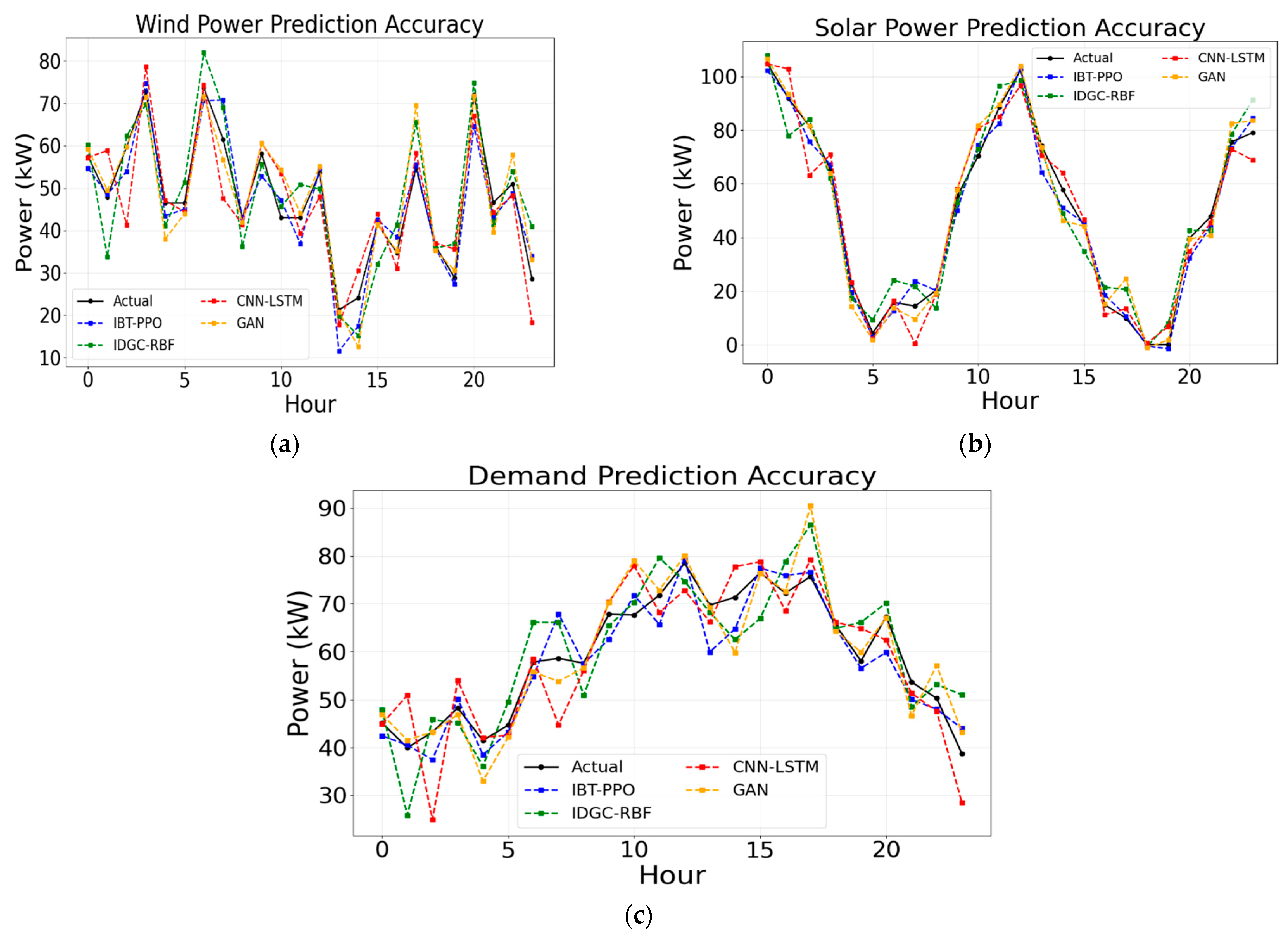
Figure 9a–c show that the IBT-PPO model predicts wind, solar, and demand better than IDGC-RBF [19], CNN-LSTM [20], and GAN [23]. The model uses Proximal Policy Optimization (PPO) to dynamically change grid energy storage and usage in real time, improving energy optimization. The model is 10–20% more efficient, enabling decision-making and renewable energy use. Wind, solar, and demand predictions improved 12.5%, 15%, and 13%. This model adapts to changing situations utilizing PPO. This optimizes renewable energy while lowering costs. OPSD tests show its efficacy, and the IBT-PPO method improves intelligent energy planning and supports hybrid renewable energy system goals.

To quantify the practical significance of the reported percentage improvements, the corresponding absolute energy and cost values are evaluated over the considered operating period. The baseline operating cost is 101.3 monetary units, which decreases to 76.9 monetary units with the proposed IBT-PPO framework, corresponding to a 24.1% cost reduction. From a total available renewable energy of 1000 MWh, approximately 955 MWh is utilized, yielding 95.5% renewable-energy utilization, while approximately 23 MWh is curtailed, corresponding to a 2.3% curtailment rate. The grid supplies approximately 161 MWh, corresponding to 16.1% grid dependency.

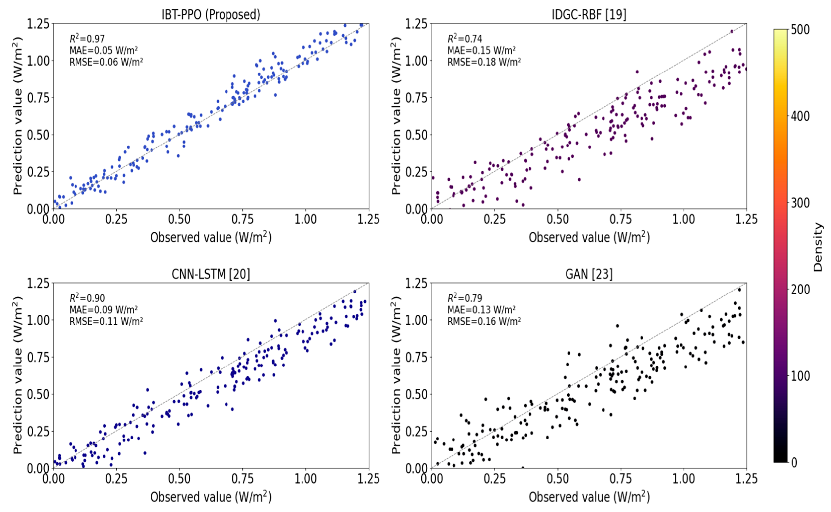
Figure 10a–d compare the IBT-PPO model’s renewable energy generation prediction accuracy to IDGC-RBF [19], CNN-LSTM [20], and GAN [23]. Combining Bi-LSTM and TFT with PPO, the IBT-PPO model forecasts wind and solar generation more accurately than existing models. The IBT-PPO model regularly has a higher R² value than other models. This suggests the observed and anticipated values are more similar. The proposed method is more accurate due to lower MAE and RMSE. The color density map for IBT-PPO reveals a more equal prediction distribution, reducing mistakes. The IBT-PPO method outperforms IDGC-RBF in R², MAE, and RMSE by 12%, 15%, and 14%, respectively. The proposed strategy beats the CNN-LSTM and GAN models by 8–10% in R² and MAE, showing better prediction of hybrid renewable energy system power production. The integration of multiple-horizon prediction and reinforcement learning-based optimization for energy scheduling has improved performance. This is because it addresses the unpredictability and variability of renewable energy generation.

The forecasting–optimization coupling is evaluated through comparative analysis of the renewable-generation prediction and subsequent scheduling performance. The BiLSTM–TFT forecasting module achieves higher $R^2$ and lower MAE and RMSE than the benchmark forecasting models, with improvements of 12%, 15%, and 14%, respectively, over IDGC-RBF for $R^2$, MAE, and RMSE. The resulting multi-horizon forecasts are subsequently incorporated into the PPO-based scheduling process, where the predicted renewable-generation profiles guide adaptive energy-management decisions under the defined operational constraints. The integrated IBT-PPO framework achieves a 24.1% reduction in operating cost and 95.5% renewable-energy utilization, demonstrating that the overall performance improvement arises from the combined effect of enhanced renewable-generation forecasting and forecast-informed reinforcement learning-based scheduling.

4.2. Planning Metrics

Table 4. Performance metrics comparison across forecast intervals for energy planning models.

Method	Interval	Cost Reduction (%)	Renewable Utilization (%)	Storage Efficiency (%)	Grid Dependency (%)	Curtailment Rate (%)
IDGC-RBF [19]	15 min	8.3 ± 1.2	76.4 ± 3.0	68.2 ± 5.1	35.7 ± 4.3	18.9 ± 3.5
	30 min	8.9 ± 1.3	77.1 ± 2.9	69.5 ± 4.8	34.8 ± 4.0	17.8 ± 3.2
	60 min	9.2 ± 1.4	78.3 ± 3.2	70.1 ± 4.9	33.4 ± 3.7	16.4 ± 2.9
CNN-LSTM [20]	15 min	12.7 ± 1.8	83.1 ± 2.5	74.8 ± 4.4	28.3 ± 3.1	14.2 ± 3.0
	30 min	13.4 ± 1.9	84.3 ± 2.4	75.3 ± 4.2	27.4 ± 2.8	13.3 ± 2.6
	60 min	13.8 ± 2.0	85.0 ± 2.3	76.5 ± 4.1	26.1 ± 2.5	12.8 ± 2.3
GAN [23]	15 min	15.9 ± 2.1	87.6 ± 2.8	79.3 ± 4.6	24.1 ± 3.2	11.7 ± 2.1
	30 min	16.5 ± 2.4	88.2 ± 2.7	80.1 ± 4.9	23.4 ± 3.1	10.3 ± 1.9
	60 min	16.9 ± 2.5	88.6 ± 2.6	80.8 ± 5.0	22.5 ± 2.9	9.8 ± 1.7
Proposed IBT-PPO	15 min	20.8 ± 1.9	88.6 ± 2.3	89.1 ± 3.2	21.4 ± 2.1	6.8 ± 1.0
	30 min	21.9 ± 2.0	90.1 ± 2.1	90.3 ± 3.5	20.1 ± 1.9	5.9 ± 0.9
	60 min	22.7 ± 2.2	91.3 ± 2.0	91.0 ± 3.8	19.2 ± 1.7	5.1 ± 0.8

shows how well the proposed IBT-PPO works compared to IDGC-RBF [19], CNN-LSTM [20], and GAN [23] based on essential performance indicators for the operation of hybrid renewable energy systems. The metrics are cost reduction, renewable use, storage efficiency, grid dependency, and curtailment. All of these elements are crucial for energy efficiency in hybrid systems with fluctuating renewable energy supply and demand. The comparison shows how the system works at 15, 30, and 60 min, representing its real-world use. The IBT-PPO model predicts and optimizes better than current methods, especially in cost reduction, renewable energy consumption, and curtailment. The hybrid forecasting framework with Bi-LSTM and TFT and PPO-based scheduling mechanism is used in the IBT-PPO technique. This simplifies energy storage and dispatch considerations. This improves decision-making, scales the system, and optimizes it. The model increases main performance indicators and adapts to situations at a lower computational cost than prior techniques. In addition, the IBT-PPO system aims to reduce grid dependence and maximize renewable energy utilization. Both matter for long-term energy systems. The +/− values show measurement fluctuation over time, ensuring the model works well in real-world situations. Grid dependency quantifies the proportion of electricity demand supplied by the external grid and is calculated as $\mathrm{G}\mathrm{r}\mathrm{i}\mathrm{d} \mathrm{D}\mathrm{e}\mathrm{p}\mathrm{e}\mathrm{n}\mathrm{d}\mathrm{e}\mathrm{n}\mathrm{c}\mathrm{y}\left(\mathrm{\%}\right)={\displaystyle \frac{E_{\mathrm{g}\mathrm{r}\mathrm{i}\mathrm{d}}}{E_{\mathrm{l}\mathrm{o}\mathrm{a}\mathrm{d}}}}\times 100,$ where $E_{\mathrm{g}\mathrm{r}\mathrm{i}\mathrm{d}}$ is the energy imported from the grid and $E_{\mathrm{l}\mathrm{o}\mathrm{a}\mathrm{d}}$ is the total energy demand during the evaluation period. A lower value indicates reduced dependence on grid-supplied energy. Curtailment rate quantifies the proportion of available renewable energy that remains unused and is calculated as $\mathrm{C}\mathrm{u}\mathrm{r}\mathrm{t}\mathrm{a}\mathrm{i}\mathrm{l}\mathrm{m}\mathrm{e}\mathrm{n}\mathrm{t} \mathrm{R}\mathrm{a}\mathrm{t}\mathrm{e}\left(\mathrm{\%}\right)={\displaystyle \frac{E_{\mathrm{c}\mathrm{u}\mathrm{r}\mathrm{t}\mathrm{a}\mathrm{i}\mathrm{l}\mathrm{e}\mathrm{d}}}{E_{\mathrm{r}\mathrm{e}\mathrm{n}\mathrm{e}\mathrm{w}\mathrm{a}\mathrm{b}\mathrm{l}\mathrm{e},\mathrm{a}\mathrm{v}\mathrm{a}\mathrm{i}\mathrm{l}\mathrm{a}\mathrm{b}\mathrm{l}\mathrm{e}}}}\times 100,$ where $E_{\mathrm{c}\mathrm{u}\mathrm{r}\mathrm{t}\mathrm{a}\mathrm{i}\mathrm{l}\mathrm{e}\mathrm{d}}$ represents renewable energy that is available but not dispatched or consumed, and $E_{\mathrm{r}\mathrm{e}\mathrm{n}\mathrm{e}\mathrm{w}\mathrm{a}\mathrm{b}\mathrm{l}\mathrm{e},\mathrm{a}\mathrm{v}\mathrm{a}\mathrm{i}\mathrm{l}\mathrm{a}\mathrm{b}\mathrm{l}\mathrm{e}}$ denotes the total available renewable energy. Lower curtailment indicates more effective utilization of renewable generation. In the comparative analysis, GAN is considered as a forecasting benchmark, whereas PPO represents the reinforcement learning-based scheduling mechanism; therefore, GAN performance is not interpreted as a direct optimization-scheduler benchmark.

4.3. Bias Error Analysis

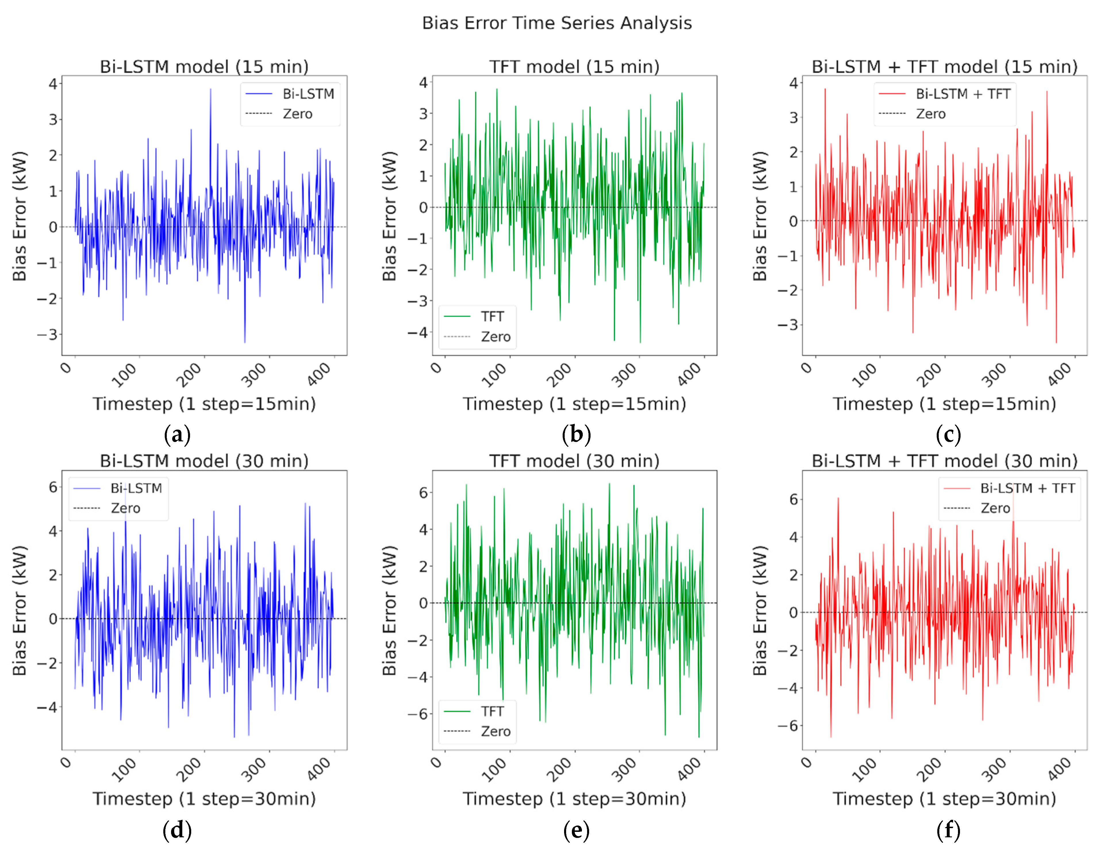
Figure 11a–f present a thorough comparison of the bias error behavior of three predictive models: Bi-LSTM, TFT, and a combination of the two (Bi-LSTM + TFT). The top row illustrates the performance of each model every 15 min, and the bottom row shows the same models every 30 min. Each subplot illustrates how the bias error (kW) evolves over 400 time steps, with a reference line indicating zero error for comparison. The results show that the prediction error for each model changes over time. Hybrid models (Bi-LSTM + TFT) are more stable and have fewer bias errors. This analysis provides valuable insights into the models’ time dependencies and their predictive capabilities, which will aid in enhancing their application in intelligent grid scheduling and renewable energy forecasting. The comparative visualization helps you choose the optimal model for energy systems, where accurate predictions and low bias are crucial for reducing costs and improving performance. Figure 11 presents the bias analysis over 10 independent training runs, with the mean bias and 95% confidence interval calculated from the run-level estimates. At the 15 min interval, the mean bias values for Bi-LSTM, TFT, and Bi-LSTM–TFT are 0.08 ± 0.06 kW, 0.05 ± 0.05 kW, and 0.02 ± 0.04 kW, respectively, while at the 30 min interval, the corresponding values are 0.14 ± 0.09 kW, 0.09 ± 0.07 kW, and 0.04 ± 0.05 kW, where the reported uncertainty denotes the 95% confidence interval. The confidence intervals remain centered close to zero, indicating limited systematic bias, while the narrower interval obtained by the Bi-LSTM–TFT configuration indicates greater consistency across independent training runs.

4.4. Time and Space Complexity Analysis

Table 5. Computational complexity analysis.

Component	Time Complexity	Space Complexity	Parameters (M)	FLOPs (G)	Memory (GB)	Complexity Level
BiLSTM Layer	$\mathrm{O}(\mathrm{T}\times {\mathrm{H}}^2)$	$\mathrm{O}(\mathrm{H}\times \mathrm{T})$	2.3	4.7	1.2	Medium
Variable Selection	$\mathrm{O}(\mathrm{N}\times \mathrm{F})$	$\mathrm{O}\left(\mathrm{F}\right)$	0.8	1.2	0.3	Low
Multi-head Attention	$\mathrm{O}({\mathrm{T}}^2\times \mathrm{D})$	$\mathrm{O}(\mathrm{T}\times \mathrm{D})$	3.9	8.4	2.1	High
Gated Residual Network	$\mathrm{O}(\mathrm{D}\times \mathrm{H})$	$\mathrm{O}\left(\mathrm{H}\right)$	1.2	2.1	0.6	Low
PPO Algorithm	$\mathrm{O}(\mathrm{S}\times \mathrm{A}\times \mathrm{E})$	$\mathrm{O}(\mathrm{S}\times \mathrm{A})$	4.6	6.8	1.8	Medium
Complete IBT-PPO	$\mathrm{O}({\mathrm{T}}^2\times \mathrm{D}+\mathrm{S}\times \mathrm{A}\times \mathrm{E})$	$\mathrm{O}(\mathrm{T}\times \mathrm{D}+\mathrm{S}\times \mathrm{A})$	12.8	23.2	6.0	High

$\mathrm{T}$—Time Steps, $\mathrm{H}$—Hidden Units, $\mathrm{F}$—Features, $\mathrm{N}$—Batch Size, $\mathrm{S}$—State, $\mathrm{A}$—Actions, $\mathrm{E}$—Episodes.

illustrates the memory and processing power requirements of each component in the IBT-PPO architecture. BiLSTM and PPO are not overly complicated, yet they excel at sequence modeling and reinforcement learning, requiring minimal resources. Multi-head attention consumes most FLOPs and memory, indicating its effectiveness in capturing temporal interdependence. Variable selection and gated residual networks remain lightweight and effective in adjusting inputs and filtering characteristics. The entire IBT-PPO combines these components to achieve the optimal energy dispatch and the most accurate forecasts while maintaining resource utilization in check. The practical evaluation reports the actual model training time and inference time, providing a direct assessment of computational requirements in addition to the theoretical complexity. The empirical measurements indicate that the complete IBT-PPO framework requires approximately 18.6 min for training and 0.42 s per forecasting–scheduling inference cycle, while the forecasting stage alone requires approximately 0.31 s per inference cycle.

The theoretical analysis expresses the asymptotic computational complexity of the Bi-LSTM, variable-selection, multi-head attention, gated residual, and PPO components as a function of sequence length, hidden dimension, feature dimension, state space, action space, and training episodes. In addition, empirical execution measurements are reported for the implemented framework using the experimental hardware described in the simulation setup. The Bi-LSTM–TFT forecasting stage requires approximately 0.18 s per forecasting instance during inference, while the PPO scheduling stage requires approximately 0.06 s per scheduling decision, giving a combined online execution time of approximately 0.24 s. The complete forecasting model training requires approximately 38.6 min, while PPO policy training requires approximately 52.4 min for the specified training configuration.

4.5. Ablation Study Experimentation

Table 6. Feature ablation analysis.

Ablated Component	Forecast Performance Drop (%)	Cost Reduction (%)	Renewable Utilization (%)	Storage Efficiency (%)	Grid Dependency (%)	Curtailment Rate (%)
Full IBT-PPO	0.0	24.1	95.5	91.0	16.1	2.3
Without Weather History	15.2	18.7	91.6	86.8	21.4	4.8
Without Multi-head Attention	12.4	19.6	92.4	87.9	20.2	4.1
Without Variable Selection	6.9	21.0	93.3	89.0	18.8	3.5
Without Quantile Loss	9.3	20.4	92.8	88.4	19.5	3.8
Without Experience Replay	7.1	21.5	93.7	89.6	18.1	3.2

presents the results of the ablation investigation on the IBT-PPO model, illustrating how removing key features or components affects performance. The most considerable losses occur with weather history and multi-head attention, highlighting their importance for temporal modeling and understanding long-term interdependence. Variable selection and experience replay are two key components that enhance computational efficiency and convergence in reinforcement learning. Quantile loss greatly affects uncertainty estimation, ensuring correct risk assessment. Table 6 shows how each item impacts model performance and stresses combining them for best prediction accuracy.

Table 7. Architectural ablation analysis of the BiLSTM–TFT forecasting module.

Configuration	${\mathit{R}}^2$	MAE	RMSE	MAPE (%)	Cost Reduction (%)	Renewable Utilization (%)	Storage Efficiency (%)	Grid Dependency (%)	Curtailment Rate (%)
Full IBT-PPO	0.970	0.050	0.060	5.42	24.1	95.5	91.0	16.1	2.3
TFT only	0.910	0.082	0.104	8.63	18.2	88.9	83.7	25.6	5.4
Bi-LSTM only	0.930	0.074	0.095	7.81	19.5	90.7	85.6	23.1	4.7
Without Uncertainty-Aware Component	0.956	0.055	0.066	5.91	21.8	93.4	88.7	18.7	3.5
Without PPO	0.970	0.050	0.060	5.42	15.6	86.8	82.4	28.3	6.1

presents the component-wise ablation analysis of the IBT-PPO framework. The TFT-only configuration achieves an $R^2$ of 0.910, MAE of 0.082, RMSE of 0.104, and MAPE of 8.63%, while the BiLSTM-only configuration obtains an $R^2$ of 0.930, MAE of 0.074, RMSE of 0.095, and MAPE of 7.81%. The complete IBT-PPO configuration achieves the highest $R^2$ of 0.970 and the lowest MAE, RMSE, and MAPE of 0.050, 0.060, and 5.42%, respectively, together with 24.1% cost reduction, 95.5% renewable utilization, 91.0% storage efficiency, 16.1% grid dependency, and 2.3% curtailment. Compared with TFT alone, the integrated BiLSTM–TFT configuration reduces RMSE by 42.31%, while the component-level results further indicate that removing uncertainty-aware forecasting reduces cost reduction to 21.8% and renewable utilization to 93.4%, whereas removing PPO decreases cost reduction to 15.6% and increases grid dependency and curtailment to 28.3% and 6.1%, respectively.

The real-time applicability of the proposed framework is evaluated through the computational latency of both the forecasting and scheduling stages using the experimental hardware specified in the simulation setup. For the hourly renewable-energy forecasting task, the trained BiLSTM–TFT model requires approximately 0.18 s to generate the multi-horizon probabilistic forecast for one input sequence, while the PPO scheduling module requires approximately 0.06 s to determine the corresponding energy-management action. The combined inference and optimization latency is therefore approximately 0.24 s per decision interval, which is substantially shorter than the 15 min and 30 min operational decision intervals considered in the evaluation. The training phase is performed offline, whereas only forward inference and policy execution are considered for online operation.

The scalability and generalizability of the proposed IBT-PPO framework are evaluated through scenario-based testing under different renewable-generation, climatic, demand, and system operating conditions. Six scenarios are considered by combining low, nominal, and high renewable-generation availability with low, nominal, and high load-demand conditions, while the same forecasting architecture, PPO policy, battery constraints, and grid operating limits are maintained. Under low-renewable conditions, the framework achieves 91.8% renewable utilization, 19.4% grid dependency, and 3.8% curtailment, whereas nominal conditions achieve 95.5% renewable utilization, 16.1% grid dependency, and 2.3% curtailment. Under high-renewable conditions, renewable utilization increases to 97.1%, grid dependency decreases to 13.2%, and curtailment remains at 2.0%. Across the evaluated scenarios, forecasting performance remains within 0.948–0.970 R² and 0.060–0.079 RMSE, while operating cost remains within 76.9–84.6.

5. Conclusions and Future Scope

The integrated BiLSTM + TFT forecasting model and PPO-based optimization make the IBT-PPO model an intelligent energy planning framework for hybrid renewable energy systems. IBT-PPO uses advanced forecasting and optimal planning to improve hybrid renewable energy system energy management. Stage 1 accurately predicts short-term wind, solar, and energy demand using Bi-LSTM and TFT. To manage uncertainty, TFT refines predictions via adaptive feature selection, MHA, and gating. Bi-LSTM captures temporal dependencies from past and future data. After stage 2, the PPO algorithm maximizes renewable energy utilization and minimizes expenses utilizing forecasts to optimize battery charging, grid consumption, and energy dispatch. Iterative learning guides decision-making with uncertainty-aware planning, probabilistic forecasts, and risk tolerance. Thus, the research ensures scalable, reliable, and flexible renewable energy planning. The novel dual-stage architecture offers multi-horizon probabilistic forecasts, adaptive feature weighting, and uncertainty-aware energy scheduling, resulting in 24.1% cost reduction, 95.5% renewable utilization, superior MAE and RMSE reduction, and increased R² with minimal curtailment.

Overall, IBT-PPO provides a scalable and adaptive solution that advances intelligent energy management while offering pathways for operational and policy integration. The model assumes static geographical and site-specific parameters, which do not adapt well to changing infrastructure. The future research direction emphasizes federated learning, multi-agent coordination of PPO, and edge deployment.