Economic–Environmental Dispatch of a Hybrid Microgrid Using an Improved Red-Billed Blue Magpie Optimizer

Abstract

The intermittency and seasonal variation of wind and photovoltaic generation complicate the economic–environmental dispatch of microgrids with high renewable-energy penetration. This study develops a grid-connected hybrid microgrid dispatch model that uses min–max normalization to place operating and environmental treatment costs on comparable scales. An improved red-billed blue magpie optimizer (IRBMO) is proposed to solve the resulting nonlinear optimization problem. IRBMO integrates composite chaotic initialization, an anti-predation mechanism, a multi-stage fine foraging strategy, and a simulated annealing acceptance mechanism to improve population diversity and solution accuracy while reducing the risk of becoming trapped in local optima. The algorithm is evaluated on ten CEC2019 benchmark functions and then applied to three microgrid configurations under typical summer and winter conditions. Its performance is compared with the red-billed blue magpie optimizer (RBMO), particle swarm optimization (PSO), snake optimizer (SO), dung beetle optimizer (DBO), hippopotamus optimization (HO), artificial rabbits optimization (ARO), multi-verse optimizer (MVO), and differential evolution (DE). The results show that IRBMO provides competitive solution accuracy and optimization stability. Among the three configurations, the complete system comprising photovoltaic (PV), wind turbine (WT), microturbine (MT), fuel cell (FC), and storage battery (SB) achieves the best overall dispatch performance. Its mean comprehensive costs are 1578.20 Chinese yuan (CNY) in summer and 1535.46 CNY in winter, with corresponding mean pollutant emissions of 850.66 kg and 792.51 kg. Under the profiles considered in this study, retaining both renewable sources reduces the comprehensive cost and pollutant emissions of the grid-connected microgrid.

1. Introduction

Global economic growth remains heavily dependent on fossil fuels, and this dependence continues to intensify the greenhouse effect and associated climate risks. Renewable energy development is therefore an important means of reducing dependence on fossil fuels and mitigating these environmental impacts [1]. However, renewable power generation is inherently intermittent and uncertain, resulting in variable output profiles. These fluctuations increase the risk of mismatches between power generation and load demand, which can disrupt real-time power balance and compromise the safe and reliable operation of the utility grid [2]. Microgrids can integrate distributed energy resources and coordinate their operation through optimal dispatch. Such coordination can mitigate fluctuations in renewable generation and maintain a regional balance between supply and demand, thereby reducing grid operational risks and supporting the transition toward a low-carbon energy system [3].

Management of microgrid operations primarily focuses on economic dispatch. Its goal is to optimally schedule the power outputs of distributed energy resources to minimize operating costs while satisfying load demand and system constraints [4]. However, this objective focuses solely on economic performance, which is insufficient to meet the requirements of modern power systems [5]. Therefore, economic–environmental dispatch (EED), which incorporates pollutant treatment costs into the optimization objective, balances economic and environmental objectives while satisfying operational constraints [6,7].

Microgrid optimal dispatch is characterized by high dimensionality and nonlinearity. When addressing such complex problems, conventional mathematical approaches often incur high computational costs and are prone to becoming trapped in suboptimal solutions [8,9]. Consequently, owing to their broad applicability and flexibility, metaheuristic optimization algorithms have become widely used to solve such problems [10]. Typical examples include particle swarm optimization (PSO) [11], snake optimizer (SO) [12], dung beetle optimizer (DBO) [13], hippopotamus optimization (HO) [14], artificial rabbits optimization (ARO) [15], multi-verse optimizer (MVO) [16], and differential evolution (DE) [17]. In recent years, improved metaheuristic algorithms have been widely studied for microgrid optimal dispatch problems. Lu et al. [18] proposed an enhanced sardine optimization algorithm to balance economic and environmental objectives in microgrid systems. Wang et al. [19] incorporated electric vehicles into the microgrid system and improved the reference-vector-guided evolutionary algorithm by combining a Chebyshev map with an angle penalty distance strategy, thereby reducing the system’s operating and pollutant treatment costs. With fuel costs and pollutant emissions as the optimization objectives, Aldosary [20] proposed a fractional-order fish migration algorithm and verified its effectiveness in solving the EED problem. Li et al. [21] adopted an improved marine predators algorithm (MPA) to solve the microgrid dispatch problem and reduce operating costs. Xie et al. [22] proposed a dynamic classification sparrow search algorithm that divides the population into three groups and assigns a corresponding strategy to each group. The algorithm was applied to isolated microgrid dispatch, reducing operating costs and carbon dioxide emissions. Elattar [23] proposed a modified harmony search algorithm to minimize fuel costs and pollutant emissions in a renewable-integrated microgrid. Zhao et al. [24] presented a multi-objective optimal dispatch approach that balances economic costs, renewable energy utilization, and user satisfaction in islanded microgrid dispatch. Chakraborty et al. [25] used the slime mould algorithm to optimize the economic and environmental performance of microgrids under multiple scenarios.

Existing microgrid energy management predominantly relies on conventional complementary wind–solar configurations. However, in practical operation, the unavailability of a single energy source due to equipment maintenance or sudden meteorological changes poses a considerable challenge to dispatch optimization. Therefore, it is necessary to examine the impact of different power supply configurations on scheduling results to evaluate the applicability of the dispatch strategy. Using a leader artificial rabbits optimization algorithm, Kharrich et al. designed multiple hybrid microgrid configurations for domestic loads, including configurations with both wind and solar resources and those lacking either resource [26]. Based on a non-dominated sorting nutcracker optimization algorithm, Liu et al. compared microgrid configurations containing both wind and solar resources with those lacking either resource, thereby evaluating the trade-off between economic and environmental performance across different seasons [27]. Kharrich et al. proposed an optimization method based on a movable damped wave algorithm to analyze the economic and environmental performance of four different power configurations [28]. Based on improved harris hawks optimization, Mallikarjun et al. compared the economic dispatch performance of a microgrid integrated with a wireless electric vehicle battery charging system under different configurations, such as wind–solar–storage complementarity and renewable energy disconnection [29]. Yakout et al. proposed an optimization framework for sizing and dispatch based on arctic puffin optimization and compared a wind–solar–storage–diesel configuration with one without photovoltaic (PV) generation [30].

Therefore, optimization algorithms should be specifically improved according to the characteristics of the problem being addressed. Based on the above studies, this study proposes an improved variant of the red-billed blue magpie optimizer (RBMO), referred to as IRBMO, to solve the economic–environmental dispatch problem of a hybrid microgrid. The main contributions of this work are summarized as follows:

1.

A grid-connected hybrid microgrid EED model is established by integrating PV, wind turbines (WT), micro-turbines (MT), fuel cells (FC), and storage batteries (SB). The model jointly considers fuel cost, operation and maintenance cost, grid interaction cost, and pollutant treatment cost, thereby enabling coordinated optimization between economic operation and environmental protection.

2.

IRBMO is proposed to solve the nonlinear microgrid dispatch problem. Composite chaotic initialization, an anti-predation mechanism, a multi-stage refined foraging strategy, and a simulated annealing acceptance criterion are incorporated to enhance population diversity, convergence accuracy, and the ability to avoid local optima.

3.

IRBMO is evaluated on the CEC2019 benchmark functions against eight optimizers: RBMO, PSO, SO, DBO, HO, ARO, MVO, and DE. The Wilcoxon and Friedman tests are used to assess statistical significance, while sensitivity analysis and component-wise ablation experiments are conducted to further evaluate the performance of IRBMO.

4.

Three microgrid configurations—namely, PV-WT-MT-FC-SB, WT-MT-FC-SB, and PV-MT-FC-SB—are constructed to evaluate the influence of different renewable energy configurations on dispatch performance. The comparative results confirm that the complete PV-WT-MT-FC-SB system provides the most economical and environmentally friendly operation scheme under the coordination of IRBMO.

The subsequent parts of this work are arranged as follows: Section 2 describes the modeling of the microgrid components, along with the objective functions and constraints. Section 3 details the underlying principles of IRBMO. Section 4 evaluates the performance of IRBMO. Section 5 presents the simulation results of the microgrid EED. Section 6 outlines the conclusions of this research.

2. Microgrid Composition and Modeling

2.1. Structural Framework of the Microgrid

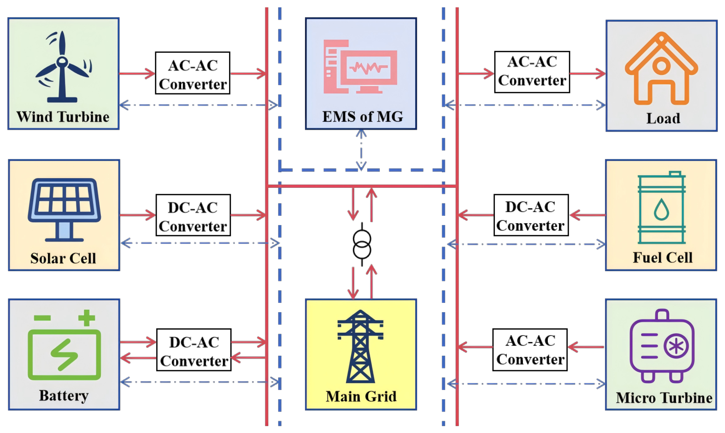
The microgrid illustrated in Figure 1 integrates PV, WT, MT, FC, and SB. These units are connected to the microgrid bus through their respective power converters to support stable power conversion and transmission. In the figure, the solid red lines indicate energy flow, whereas the dashed blue lines represent real-time communication and control links between the energy management system and individual units.

2.1.1. Photovoltaic

PV relies on semiconductor materials to transform sunlight into electricity. Solar irradiance and temperature are the primary factors determining the output power [31]:

$$\begin{array}{c}{T}_{\mathrm{c}}=T_{\mathrm{amb}}+\left({\displaystyle \frac{G_{\mathrm{AC}}(\mathrm{NOCT}-20)}{800}}\right)\end{array}$$

(1)

$$\begin{array}{c}{P}_{\mathrm{PV}}=P_{\mathrm{STC}}{\displaystyle \frac{G_{\mathrm{AC}}}{G_{\mathrm{STC}}}}(1+k(T_{\mathrm{c}}-T_{\mathrm{ref}}))\end{array}$$

(2)

where $T_{\mathrm{c}}$ is the operating temperature; $T_{\mathrm{amb}}$ is the ambient temperature; $G_{\mathrm{AC}}$ is the solar irradiance; $\mathrm{NOCT}$ is the nominal cell temperature; $P_{\mathrm{STC}}$ is the maximum power of PV under standard test conditions (STC); $G_{\mathrm{STC}}$ is the solar irradiance under STC; k is the PV power temperature coefficient; and $T_{\mathrm{ref}}$ is the reference temperature.

2.1.2. Wind Turbine

The electrical power generated by a WT is obtained by converting the kinetic energy of the wind. Its output power mainly depends on the aerodynamic parameters of the turbine and the wind speed at hub height [32]:

$$P_{\mathrm{WT}}=\left\{\begin{array}{cc}0\hfill & v<v_{\mathrm{ci}},\hspace{1em}v>v_{\mathrm{co}}\hfill \\ {\displaystyle \frac{P_{\mathrm{r}}(v-v_{\mathrm{ci}})}{v_{\mathrm{r}}-v_{\mathrm{ci}}}}\hfill & v_{\mathrm{ci}}<v<v_{\mathrm{r}}\hfill \\ P_{\mathrm{r}}\hfill & v_{\mathrm{r}}<v<v_{\mathrm{co}}\hfill \end{array}\right.$$

(3)

where $P_{\mathrm{r}}$ is the rated power of the WT; $v_{\mathrm{ci}}$, $v_{\mathrm{r}}$, and $v_{\mathrm{co}}$ are the cut-in, rated, and cut-out wind speeds, respectively; and v is the current hub-height wind speed.

2.1.3. Micro-Turbine

MT is a generation unit that uses fuels to generate electricity. It offers high reliability and efficiency, with relatively low pollutant emissions. Moreover, unlike renewable energy generation units, its output can be flexibly controlled to meet dispatch requirements [33]. Its operating efficiency as a function of output power is given by [34]:

$$\begin{array}{c}{\eta }_{\mathrm{MT}}\left(t\right)=0.0753{\left[{\displaystyle \frac{P_{\mathrm{MT}}\left(t\right)}{65}}\right]}^3-0.3095{\left[{\displaystyle \frac{P_{\mathrm{MT}}\left(t\right)}{65}}\right]}^2+0.4174{\displaystyle \frac{P_{\mathrm{MT}}\left(t\right)}{65}}+0.1068\end{array}$$

(4)

$$\begin{array}{c}{C}_{\mathrm{MT}}={\displaystyle \frac{C_{\mathrm{ng}}}{{\mathrm{LHV}}_{\mathrm{ng}}}}{\displaystyle \sum _{t=1}^T}{\displaystyle \frac{P_{\mathrm{MT}}\left(t\right)\Delta t}{{\eta }_{\mathrm{MT}}\left(t\right)}}\end{array}$$

(5)

where ${\eta }_{\mathrm{MT}}\left(t\right)$ is the operating efficiency of MT during time interval t; $C_{\mathrm{MT}}$ is the fuel cost of the MT; $C_{\mathrm{ng}}$ is the price of natural gas; ${\mathrm{LHV}}_{\mathrm{ng}}$ is the lower heating value of natural gas; $P_{\mathrm{MT}}$ is the output power of MT; T is the total number of dispatch intervals; and $\Delta t$ is the duration of each dispatch interval.

2.1.4. Fuel Cell

FC is a power generation device that converts the chemical energy of a fuel and an oxidant directly into electrical energy through electrochemical reactions [35]. Compared with conventional combustion-based generators, it produces relatively low pollutant emissions. Its fuel cost depends mainly on its output power [36]:

$$\begin{array}{c}{\eta }_{\mathrm{FC}}\left(t\right)=-0.0023P_{\mathrm{FC}}\left(t\right)+0.674\end{array}$$

(6)

$$\begin{array}{c}{C}_{\mathrm{FC}}={\displaystyle \frac{C_{\mathrm{ng}}}{{\mathrm{LHV}}_{\mathrm{ng}}}}{\displaystyle \sum _{t=1}^T}{\displaystyle \frac{P_{\mathrm{FC}}\left(t\right)\Delta t}{{\eta }_{\mathrm{FC}}\left(t\right)}}\end{array}$$

(7)

where $C_{\mathrm{FC}}$ is the fuel cost of FC; ${\eta }_{\mathrm{FC}}\left(t\right)$ is the efficiency of FC; and $P_{\mathrm{FC}}$ is the output power of FC.

2.1.5. Storage Battery

As an energy storage unit in the microgrid, SB mitigates the effects of fluctuations in WT and PV output on the utility grid [37]. The energy level of SB is represented by the state of charge (SOC), which is calculated as follows:

$$\mathrm{SOC}\left(t\right)=\left\{\begin{array}{cc}\mathrm{SOC}(t-1)+{\eta }_{\mathrm{c}}{P}_{\mathrm{SB}}\left(t\right){\displaystyle \frac{\Delta t}{E_{\mathrm{r}}}}\hfill & P_{\mathrm{SB}}\left(t\right)\le 0\hfill \\ \mathrm{SOC}(t-1)-P_{\mathrm{SB}}\left(t\right){\displaystyle \frac{\Delta t}{{\eta }_{\mathrm{dis}}{E}_{\mathrm{r}}}}\hfill & P_{\mathrm{SB}}\left(t\right)>0\hfill \end{array}\right.$$

(8)

where ${\eta }_{\mathrm{c}}$ is the charging efficiency; ${\eta }_{\mathrm{dis}}$ is the discharging efficiency; $P_{\mathrm{SB}}$ is the power of SB; and $E_{\mathrm{r}}$ is the rated capacity of SB.

2.2. Objective Function

The “No Free Lunch” theorem postulates that a universally superior algorithm for every optimization task does not exist [38]. Driven by the necessity to balance economic efficiency with environmental sustainability, this study formulates a microgrid scheduling framework that minimizes both operational expenses and emission treatment penalties.

To express the two cost components on a common scale, a normalized weighted-sum method is used to define the comprehensive cost objective:

$$\begin{array}{cc}\hfill minC=& \omega {\displaystyle \frac{C_1-C_{1,min}}{C_{1,max}-C_{1,min}}}+(1-\omega ){\displaystyle \frac{C_2-C_{2,min}}{C_{2,max}-C_{2,min}}}.\hfill \end{array}$$

(9)

where C is the normalized comprehensive cost; $C_{1,min}$ and $C_{1,max}$ are the lower and upper normalization bounds of operating cost $C_1$, respectively; $C_{2,min}$ and $C_{2,max}$ are the lower and upper normalization bounds of environmental governance cost $C_2$, respectively; and $\omega$ is the weighting coefficient. In this study, $\omega =0.5$, so the two cost components are assigned equal weights.

$$\begin{array}{c}{C}_1={\displaystyle \sum _{t=1}^T}\left(C_{\mathrm{fuel}}\left(t\right)+C_{\mathrm{om}}\left(t\right)+C_{\mathrm{grid}}\left(t\right)\right)\Delta t\end{array}$$

(10)

where $C_{\mathrm{fuel}}$ is the total fuel cost; $C_{\mathrm{om}}$ is the total operation and maintenance cost; and $C_{\mathrm{grid}}$ is the interaction cost.

The fuel cost mainly comprises the fuel consumption expenses during the operating cycle; namely,

$$C_{\mathrm{fuel}}\left(t\right)=C_{\mathrm{MT}}\left(t\right)+C_{\mathrm{FC}}\left(t\right)$$

(11)

The maintenance cost depends on the power of each generation unit during the operating cycle; namely,

$$C_{\mathrm{om}}\left(t\right)=K_{\mathrm{WT}}{P}_{\mathrm{WT}}\left(t\right)+K_{\mathrm{PV}}{P}_{\mathrm{PV}}\left(t\right)+K_{\mathrm{MT}}{P}_{\mathrm{MT}}\left(t\right)+K_{\mathrm{FC}}{P}_{\mathrm{FC}}\left(t\right)+K_{\mathrm{SB}}\left(|P_{\mathrm{dis}}\left(t\right)|+|P_{\mathrm{c}}\left(t\right)|\right)$$

(12)

where $K_{\mathrm{WT}}$, $K_{\mathrm{PV}}$, $K_{\mathrm{MT}}$, $K_{\mathrm{FC}}$ and $K_{\mathrm{SB}}$ are the maintenance cost coefficients; and $P_{\mathrm{dis}}\left(t\right)$ and $P_{\mathrm{c}}\left(t\right)$ are the discharging and charging power of SB.

Power interactions are executed via bidirectional electricity trading. The corresponding cost calculation is formulated as:

$$C_{\mathrm{grid}}\left(t\right)=\left\{\begin{array}{cc}{C}_{\mathrm{buy}}\left(t\right)P_{\mathrm{grid}}\left(t\right),\hfill & P_{\mathrm{grid}}\left(t\right)\ge 0\hfill \\ C_{\mathrm{sell}}\left(t\right)P_{\mathrm{grid}}\left(t\right),\hfill & P_{\mathrm{grid}}\left(t\right)<0\hfill \end{array}\right.$$

(13)

where $C_{\mathrm{buy}}\left(t\right)$ and $C_{\mathrm{sell}}\left(t\right)$ respectively denote the tariffs for importing and exporting electricity with the external utility during interval t. Here, the emissions associated with electricity purchased from the main grid are included in the environmental governance cost. Electricity exported to the main grid is accounted for only as sales revenue and is not used to offset the cost.

The environmental governance cost is the treatment expense for gaseous pollutants:

$$C_2={\displaystyle \sum _{t=1}^T}{\displaystyle \sum _{i=1}^I}{\displaystyle \sum _{k=1}^K}{\alpha }_k{\beta }_{i,k}{P}_i\left(t\right)\Delta t$$

(14)

where ${\alpha }_k$ is the cost required to treat a unit mass of pollutant type k; ${\beta }_{i,k}$ is the emission coefficient of generation unit i for pollutant type k; I represents the total number of generation units included in the emission calculation; and K represents the total number of pollutant types—namely, ${\mathrm{CO}}_2$, ${\mathrm{SO}}_2$, and ${\mathrm{NO}}_x$.

2.3. Constraints

The total generated power of the system must achieve a dynamic balance with the total power consumption; namely,

$$P_{\mathrm{load}}\left(t\right)=P_{\mathrm{WT}}\left(t\right)+P_{\mathrm{PV}}\left(t\right)+P_{\mathrm{MT}}\left(t\right)+P_{\mathrm{FC}}\left(t\right)+P_{\mathrm{grid}}\left(t\right)+P_{\mathrm{SB}}\left(t\right)$$

(15)

where $P_{\mathrm{load}}\left(t\right)$ is the load power of the system.

WT, PV, MT, and FC units are restricted by the active power constraints given below:

$$\begin{array}{c}{P}_{i,min}\le P_i\left(t\right)\le P_{i,max}\end{array}$$

(16)

$$\begin{array}{c}-R_i^{\mathrm{down}}\Delta t\le P_i^{\mathrm{CG}}\left(t\right)-P_i^{\mathrm{CG}}(t-1)\le R_i^{\mathrm{up}}\Delta t\end{array}$$

(17)

where $P_{i,min}$ and $P_{i,max}$ represent the extreme output power of generation unit i; $\mathrm{CG}$ represents the controllable generation units; and $R_i^{\mathrm{down}}$ and $R_i^{\mathrm{up}}$ dictate the ascending and descending ramp limits.

The limits regarding the state of charge and power exchange of SB must satisfy:

$$\left\{\begin{array}{c}{\mathrm{SOC}}_{min}\le \mathrm{SOC}\left(t\right)\le {\mathrm{SOC}}_{max},\hfill \\ P_{\mathrm{SB},min}\le P_{\mathrm{SB}}\left(t\right)\le P_{\mathrm{SB},max},\hfill \\ \mathrm{SOC}\left(24\right)=\mathrm{SOC}\left(0\right)\hfill \end{array}\right.$$

(18)

The interaction power constraints are as follows:

$$P_{\mathrm{grid},min}\le P_{\mathrm{grid}}\left(t\right)\le P_{\mathrm{grid},max}$$

(19)

The fitness evaluation and constraint-handling procedure used for microgrid dispatch optimization is described in Appendix A.

3. Improved Red-Billed Blue Magpie Optimizer Algorithm

3.1. Red-Billed Blue Magpie Optimizer

As a swarm-based metaheuristic algorithm, RBMO is inspired by the coordinated foraging behavior of red-billed blue magpies in nature. Its mathematical model includes three main behavioral processes: searching for food, attacking prey, and storing food [39].

When searching for food, red-billed blue magpies usually move in either small or large flocks. The search behavior of a small flock is modeled by Equation (20), while the wide-area exploration behavior of a large flock is described by Equation (21):

$$\begin{array}{c}{X}_i(t+1)=X_i\left(t\right)+\left[{\displaystyle \frac{1}{p}}·{\displaystyle \sum _{m=1}^p}{X}^m\left(t\right)-X^{\mathrm{rs}}\left(t\right)\right]·{\mathrm{rand}}_1\end{array}$$

(20)

$$\begin{array}{c}{X}_i(t+1)=X_i\left(t\right)+\left[{\displaystyle \frac{1}{q}}·{\displaystyle \sum _{m=1}^q}{X}^m\left(t\right)-X^{\mathrm{rs}}\left(t\right)\right]·{\mathrm{rand}}_2\end{array}$$

(21)

where $X_i\left(t\right)$ is the position of the current individual; $X^{\mathrm{rs}}\left(t\right)$ is the position of a randomly selected individual; $X^m\left(t\right)$ is the position of the randomly selected individual m; and p and q are the numbers of magpies in the small and large flocks, respectively. Specifically, p and q are randomly generated integers in $[2,5]$ and $[10,N]$, respectively, where N is the total population size. The switching parameter $\epsilon$ is set to $0.5$. If $\mathrm{rand}<\epsilon$, the small-flock strategy is selected; otherwise, the large-flock strategy is selected.

After detecting prey, red-billed blue magpies use different attack strategies depending on flock size. For a small flock, the pecking behavior toward small prey is modeled by Equation (22). For a large flock, the besieging behavior toward large prey is modeled by Equation (23). The nonlinear control factor $\mathrm{CF}$ is defined in Equation (24):

$$\begin{array}{c}{X}_i(t+1)=X_{\mathrm{food}}\left(t\right)+\mathrm{CF}·\left({\displaystyle \frac{1}{p}}{\displaystyle \sum _{m=1}^p}{X}^m\left(t\right)-X_i\left(t\right)\right)·{\mathrm{randn}}_1\end{array}$$

(22)

$$\begin{array}{c}{X}_i(t+1)=X_{\mathrm{food}}\left(t\right)+\mathrm{CF}·\left({\displaystyle \frac{1}{q}}{\displaystyle \sum _{m=1}^q}{X}^m\left(t\right)-X_i\left(t\right)\right)·{\mathrm{randn}}_2\end{array}$$

(23)

$$\begin{array}{c}\mathrm{CF}={\left(1-{\displaystyle \frac{t}{T}}\right)}^{2\times {\displaystyle \frac{t}{T}}}\end{array}$$

(24)

where $X_{\mathrm{food}}\left(t\right)$ is the position of the optimal individual in the current iteration; $\mathrm{CF}$ decreases monotonically from approximately 1 to 0 as the iterations progress. A large $\mathrm{CF}$ allows wider position perturbations around $X_{\mathrm{food}}\left(t\right)$ to maintain population diversity, whereas a small $\mathrm{CF}$ narrows the attack radius and guides individuals toward the optimal solution.

Finally, RBMO simulates the food-storing behavior of red-billed blue magpies by retaining better candidate solutions through a greedy selection mechanism. The corresponding update rule is as follows:

$$X_i(t+1)=\left\{\begin{array}{cc}{X}_i\left(t\right),\hfill & {\mathrm{fitness}}_{\mathrm{old}}^i<{\mathrm{fitness}}_{\mathrm{new}}^i\hfill \\ X_i(t+1),\hfill & else\hfill \end{array}\right.$$

(25)

where ${\mathrm{fitness}}_{\mathrm{old}}^i$ and ${\mathrm{fitness}}_{\mathrm{new}}^i$ are the fitness values of individual i before and after the position update.

3.2. Proposed IRBMO

Although RBMO has demonstrated better optimization performance than traditional algorithms, its computational efficiency and solution accuracy remain limited for high-dimensional or large-scale complex optimization problems [40]. To address these limitations, this study proposes IRBMO, which integrates multiple mechanisms throughout the optimization process.

3.2.1. Composite Chaotic Mapping Strategy

RBMO uses random population initialization, which may provide insufficient coverage of the search space and produce an uneven distribution of candidate solutions within the feasible region. This can reduce convergence speed and solution accuracy. To address this limitation, a composite chaotic map is used to generate the initial population, as defined in Equation (26):

$$X_i=\mathrm{lb}+M(\alpha ,z_i)·(\mathrm{ub}-\mathrm{lb})$$

(26)

where $\mathrm{ub}$ and $\mathrm{lb}$ are the upper and lower bounds of the solution space; and $M(\alpha ,z_i)$ is the composite chaotic mapping strategy.

The composite chaotic mapping strategy uses the control parameter $\alpha$ to balance the contributions of the Cubic and Sine maps. The Cubic, Sine, and composite maps are defined in Equations (27), (28), and (29), respectively.

$$\begin{array}{c}{z}_{i+1}^{\mathrm{C}}=a{z}_i\left(1-z_i^2\right)\end{array}$$

(27)

$$\begin{array}{c}{z}_{i+1}^{\mathrm{S}}={\displaystyle \frac{b}{4}}\sin \left(\pi z_i\right)\end{array}$$

(28)

$$\begin{array}{c}{z}_{i+1}^{\mathrm{CS}}=\sin \left\{\pi \left[\alpha z_{i+1}^{\mathrm{C}}+(1-\alpha )z_{i+1}^{\mathrm{S}}\right]\right\}\end{array}$$

(29)

where $z_i$ is the chaotic variable at the current iteration; $z_{i+1}^{\mathrm{C}}$ and $z_{i+1}^{\mathrm{S}}$ are the intermediate outputs of the Cubic and Sine maps, respectively; and $z_{i+1}^{\mathrm{CS}}$ is the final output of the composite chaotic map. The weighting coefficient $\alpha$ is set to $0.5$ to balance the contributions of the two maps, while $a=2.595$ and $b=4$ are the control parameters of the Cubic and Sine maps, respectively.

3.2.2. Anti-Predation Strategy

RBMO models the foraging behavior of different flock sizes using Equations (20) and (21). However, this single exploration mode may be insufficient for complex multimodal optimization problems, increasing the risk of premature stagnation and making the global optimum more difficult to locate. To improve exploration, IRBMO introduces an anti-predation mechanism inspired by natural behavior.

Red-billed blue magpies face natural predators such as eagles, falcons, and cats, and their evasion tactics depend on flock size. A small flock scatters randomly to confuse predators, as described in Equation (30), whereas a large flock uses its collective advantage to move toward the safest known region, as described in Equation (31). For each individual, Equation (20) or Equation (21) generates a conventional food-searching candidate $X_{\mathrm{RBMO},i}\left(t\right)$ according to the selected flock strategy. Under the same strategy, Equation (30) or Equation (31) generates the corresponding anti-predation candidate $X_{\mathrm{APS},i}\left(t\right)$. After boundary handling, the objective function evaluates the fitness of both candidates, and Equation (33) selects the better one. In conventional RBMO, Equation (25) then determines whether this candidate or the historically stored position is retained. IRBMO replaces this greedy storage rule with the dynamic food-storage mechanism in Equations (37) and (38). The retained position becomes the current position $X_i\left(t\right)$ for subsequent operations.

$$\begin{array}{c}{X}_{\mathrm{APS},i}\left(t\right)=X_i\left(t\right)-M·\left({\mathrm{lb}}^{\mathrm{ap}}+\mathrm{rand}·({\mathrm{ub}}^{\mathrm{ap}}-{\mathrm{lb}}^{\mathrm{ap}})\right)\end{array}$$

(30)

$$\begin{array}{c}{X}_{\mathrm{APS},i}\left(t\right)=X_i\left(t\right)+\mathrm{rand}·\left(X_{\mathrm{food}}\left(t\right)-M·X_i\left(t\right)\right)\end{array}$$

(31)

$$\begin{array}{c}M=\mathrm{round}\left(1+z_{i+1}^{\mathrm{CS}}\right)\end{array}$$

(32)

$$\begin{array}{c}{X}_i(t+1)=\left\{\begin{array}{cc}{X}_{\mathrm{APS},i}\left(t\right),\hfill & \mathrm{if} f_{\mathrm{APS},i}\left(t\right)<f_{\mathrm{RBMO},i}\left(t\right),\hfill \\ X_{\mathrm{RBMO},i}\left(t\right),\hfill & \mathrm{otherwise}.\hfill \end{array}\right.\end{array}$$

(33)

where $X_{\mathrm{APS},i}\left(t\right)$ and $X_{\mathrm{RBMO},i}\left(t\right)$ are the anti-predation candidate position and the conventional food-searching candidate position of individual i at iteration t, respectively; $f_{\mathrm{APS},i}\left(t\right)=f\left(X_{\mathrm{APS},i}\left(t\right)\right)$ and $f_{\mathrm{RBMO},i}\left(t\right)=f\left(X_{\mathrm{RBMO},i}\left(t\right)\right)$ are their respective fitness values, where $f(·)$ is the objective function. For the minimization problem considered in this study, the candidate with the smaller fitness value is selected as $X_i(t+1)$. The terms ${\mathrm{lb}}^{\mathrm{ap}}=\mathrm{lb}/t$ and ${\mathrm{ub}}^{\mathrm{ap}}=\mathrm{ub}/t$ are the escape-search boundaries that shrink with the iteration number, and M is a positive integer generated by the composite chaotic mapping strategy.

3.2.3. Multi-Stage Fine Foraging Strategy

As shown in Equations (22) and (23), RBMO uses the optimal individual as the search center and attacks prey within its neighborhood. However, excessive dependence on the best-performing individual can limit local refinement. To address this limitation, the Brownian motion and Lévy flight rules from the three-stage movement mechanism of MPA [41] are adapted to construct a multi-stage fine foraging strategy for the attack stage of RBMO.

Following the three-stage mechanism of MPA, the exploitation process is divided into three periods. In the early stage, the population uses Brownian motion with relatively stable step sizes to approach food-rich regions, and positions are updated using Equation (34). In the middle stage, the population is divided into two equal subgroups to balance exploration and exploitation. As shown in Equation (35), the first subgroup uses Lévy flight to explore peripheral regions, while the second uses Brownian motion for local exploitation with a gradually shrinking foraging radius. In the late stage, the population uses the exploitation capability of Lévy flight to search near the optimal food source, as shown in Equation (36). IRBMO embeds this MPA-derived three-stage movement mechanism into the attack process of RBMO to form a multi-stage position-update strategy.

$$\begin{array}{c}{X}_i(t+1)=X_i\left(t\right)+P·\mathrm{rand}·\left[R_{\mathrm{B}}·(X_{\mathrm{food}}\left(t\right)-R_{\mathrm{B}}·X_i\left(t\right))\right], t<{\displaystyle \frac{T}{3}}\end{array}$$

(34)

$$\begin{array}{c}{X}_i(t+1)=\left\{\begin{array}{cc}{X}_i\left(t\right)+P·\mathrm{rand}·\left[R_{\mathrm{L}}·(X_{\mathrm{food}}\left(t\right)-R_{\mathrm{L}}·X_i\left(t\right))\right],\hfill & i\le N/2\hfill \\ X_{\mathrm{food}}\left(t\right)+P·\mathrm{CF}·\left[R_{\mathrm{B}}·(R_{\mathrm{B}}·X_{\mathrm{food}}\left(t\right)-X_i\left(t\right))\right],\hfill & i>N/2\hfill \end{array}\right., {\displaystyle \frac{T}{3}}<t<{\displaystyle \frac{2}{3}}T\end{array}$$

(35)

$$\begin{array}{c}{X}_i(t+1)=X_{\mathrm{food}}\left(t\right)+P·\mathrm{CF}·\left[R_{\mathrm{L}}·(R_{\mathrm{L}}·X_{\mathrm{food}}\left(t\right)-X_i\left(t\right))\right], {\displaystyle \frac{2}{3}}T<t\end{array}$$

(36)

where $R_{\mathrm{B}}$ is the Brownian motion vector following a standard normal distribution; $R_{\mathrm{L}}$ is the Lévy flight vector; P is a constant coefficient controlling the step size. In Equation (35), $\mathrm{CF}$ contracts the foraging radius generated by Brownian motion for the second subgroup, while the first subgroup retains the peripheral exploration capability provided by Lévy flight. In Equation (36), the decrease in $\mathrm{CF}$ reduces the perturbation generated by Lévy flight and promotes fine exploitation around $X_{\mathrm{food}}\left(t\right)$, improving convergence accuracy.

3.2.4. Simulated Annealing

As shown in Equation (25), RBMO uses a greedy selection mechanism during the food-storage phase. Because this mechanism directly rejects inferior solutions, it can restrict the exploration of potentially useful regions. Therefore, IRBMO incorporates simulated annealing into a new food-storage mechanism.

Equation (37) defines a temperature parameter that decreases nonlinearly with the iterations to represent the changing survival pressure on red-billed blue magpies across foraging seasons. When a newly explored position has lower food abundance, it is not immediately discarded. Instead, Equation (38) applies the Metropolis criterion and accepts the position as an alternative food-storage point with probability $\lambda \left(t\right)$ to reduce the risk of becoming trapped in a local optimum.

$$\begin{array}{c}\mathrm{Temp}\left(t\right)=max\left\{{\epsilon }_{\mathrm{T}}, 0.1 f_{\mathrm{avg}}\left(t\right){\left(1-{\displaystyle \frac{t}{T_{max}}}\right)}^2\right\},\end{array}$$

(37)

$$\begin{array}{c}\lambda \left(t\right)=min\left\{1, \exp \left[-{\displaystyle \frac{f\left(X^{\mathrm{new}}\right)-f\left(X^{\mathrm{old}}\right)}{\mathrm{Temp}\left(t\right)}}\right]\right\},\end{array}$$

(38)

where $\mathrm{Temp}\left(t\right)$ is the temperature parameter; $f_{\mathrm{avg}}\left(t\right)$ is the average fitness; $\lambda \left(t\right)$ is the probability of accepting a new solution; and $X^{\mathrm{new}}$ and $X^{\mathrm{old}}$ are the new and old food-storage points.

3.3. Optimization System Flowchart

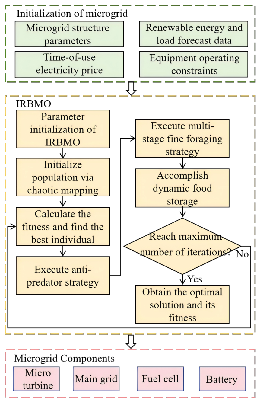
Figure 2 shows the optimal dispatch process of the microgrid. The microgrid integrates various distributed energy resources, and its dispatch strategy considers time-of-use electricity prices and seasonal variations in renewable energy output. IRBMO is used to solve the resulting optimization problem by minimizing the comprehensive cost subject to the system’s operational constraints.

The pseudocode of IRBMO is shown in Algorithm 1.

Algorithm 1 Pseudo-code of IRBMO

Input:  population size N, maximum iterations T, the lower bounds $\mathrm{lb}$ and the upper bounds $\mathrm{ub}$ Output:  the optimal solution $X_{\mathrm{food}}$ and its fitness   1: Initialize population using Chaos Sequence by Equation (26)   2: Calculate fitness for each search agent and update $X_{\mathrm{food}}$   3: $t=1$   4: while  $t\le T$  do   5:    Compute adaptive bounds ${\mathrm{lb}}^{\mathrm{ap}}$ and ${\mathrm{ub}}^{\mathrm{ap}}$   6:    for $i=1:N$ do   7:       Calculate the mean positions of the generated small and large groups   8:       Generate the chaotic factor M using Equation (32)   9:       if $\mathrm{rand}<0.5$ then 10:          Generate $X_{\mathrm{RBMO},i}\left(t\right)$ using Equation (20) and $X_{\mathrm{APS},i}\left(t\right)$ using Equation (30) 11:       else 12:          Generate $X_{\mathrm{RBMO},i}\left(t\right)$ using Equation (21) and $X_{\mathrm{APS},i}\left(t\right)$ using Equation (31) 13:       end if 14:       Check boundaries 15:       Updating $X_i(t+1)$ by greedy selection using Equation (33) 16:       Update current Best Value and $X_{\mathrm{food}}$ 17:    end for 18:    Calculate non-linear parameter $\mathrm{CF}$ using Equation (24) 19:    for $i=1:N$ do 20:       Generate Brownian motion and Lévy flight 21:       if $t<T/3$ then 22:          Updating $X_i(t+1)$ using Equation (34) 23:       else if $T/3\le t<2T/3$ then 24:          Updating $X_i(t+1)$ using Equation (35) 25:       else 26:          Updating $X_i(t+1)$ using Equation (36) 27:       end if 28:       Check boundaries, evaluate fitness, update Best Value and $X_{\mathrm{food}}$ 29:    end for 30:    Accomplish Dynamic Food Storage using Equation (38) 31:    $t=t+1$ 32: end while

4. Performance Evaluation and Discussion

4.1. Experimental Parameter Settings

To validate the efficacy of IRBMO, it is benchmarked against the following optimizers: RBMO, PSO, SO, DBO, HO, ARO, MVO, and DE. To ensure fair comparisons, the swarm size and the maximum number of iterations are set to 50 and 500 across all tests. The specific internal parameters configured for each algorithm are detailed in

Table 1. Parameter settings for each algorithm.

Algorithm	Parameter
IRBMO	$\epsilon =0.5$
RBMO	$\epsilon =0.5$
PSO	$\omega =0.9;c_1=c_2=1.5$
SO	$c_1=0.5;c_2=0.05;c_3=2$
DBO	$k=0.1;b=0.3;s=0.5$
HO	$\beta =1.5$
ARO	No additional control parameters
MVO	${\mathrm{WEP}}_{min}=0.2;{\mathrm{WEP}}_{max}=1;p=6$
DE	$F\in [0.2,0.8]; \mathrm{CR}=0.2$

Note: RBMO, red-billed blue magpie optimizer; PSO, particle swarm optimization; SO, snake optimizer; DBO, dung beetle optimizer; HO, hippopotamus optimization; ARO, artificial rabbits optimization; MVO, multi-verse optimizer; DE, differential evolution; WEP, wormhole existence probability; CR, crossover rate.

. Furthermore, to obtain statistically reliable results, every method undergoes 30 independent runs per function.

The experiments employ the CEC2019 benchmark test suite, which comprises three real-world-inspired problems with fixed dimensions and seven shifted and rotated classical functions [42]. Ten functions are employed to comprehensively evaluate the convergence accuracy, global search capability, and optimization stability of the algorithms.

4.2. Performance Analysis on Test Functions

All experiments are implemented in MATLAB R2023a and conducted on a Windows 11 (64-bit) PC with an Intel i5-10400 CPU (2.90 GHz) and 16 GB RAM.

Table 2. Statistical results of all algorithms on the ten CEC2019 benchmark functions.

Function	Algorithm	Best	Worst	Mean	Median	Std
F1	IRBMO	$1.0000\times {10}^0$	$1.0000\times {10}^0$	$1.0000\times {10}^0$	$1.0000\times {10}^0$	$5.8312\times {10}^{-17}$
	RBMO	$1.0000\times {10}^0$	$1.1135\times {10}^0$	$1.0242\times {10}^0$	$1.0119\times {10}^0$	$2.9727\times {10}^{-2}$
	SO	$1.0000\times {10}^0$	$4.8907\times {10}^5$	$3.1434\times {10}^4$	$3.3009\times {10}^3$	$9.1718\times {10}^4$
	PSO	$6.8402\times {10}^3$	$1.9593\times {10}^6$	$3.8542\times {10}^5$	$2.1432\times {10}^5$	$4.5216\times {10}^5$
	DBO	$1.0000\times {10}^0$	$5.5137\times {10}^6$	$5.9494\times {10}^5$	$6.3688\times {10}^2$	$1.2111\times {10}^6$
	HO	$1.0000\times {10}^0$	$1.0000\times {10}^0$	$1.0000\times {10}^0$	$1.0000\times {10}^0$	$0.0000\times {10}^0$
	ARO	$1.0000\times {10}^0$	$1.0000\times {10}^0$	$1.0000\times {10}^0$	$1.0000\times {10}^0$	$2.8531\times {10}^{-15}$
	MVO	$3.9209\times {10}^4$	$3.6719\times {10}^6$	$1.2281\times {10}^6$	$9.6047\times {10}^5$	$1.0694\times {10}^6$
	DE	$1.0649\times {10}^6$	$1.8372\times {10}^7$	$6.1899\times {10}^6$	$6.1611\times {10}^6$	$3.4031\times {10}^6$
F2	IRBMO	$2.2690\times {10}^0$	$3.2754\times {10}^0$	$2.9731\times {10}^0$	$3.0942\times {10}^0$	$2.7804\times {10}^{-1}$
	RBMO	$3.6194\times {10}^0$	$1.5370\times {10}^1$	$8.0903\times {10}^0$	$7.6962\times {10}^0$	$2.4374\times {10}^0$
	SO	$5.0000\times {10}^0$	$4.7341\times {10}^2$	$1.8414\times {10}^2$	$1.5668\times {10}^2$	$1.4058\times {10}^2$
	PSO	$1.8735\times {10}^2$	$6.9986\times {10}^3$	$6.0870\times {10}^2$	$3.4517\times {10}^2$	$1.2175\times {10}^3$
	DBO	$4.2494\times {10}^0$	$4.6573\times {10}^3$	$6.4545\times {10}^2$	$3.9907\times {10}^2$	$1.0861\times {10}^3$
	HO	$4.9679\times {10}^0$	$5.0000\times {10}^0$	$4.9989\times {10}^0$	$5.0000\times {10}^0$	$5.8688\times {10}^{-3}$
	ARO	$4.0529\times {10}^0$	$4.2968\times {10}^0$	$4.2402\times {10}^0$	$4.2512\times {10}^0$	$5.1587\times {10}^{-2}$
	MVO	$1.5407\times {10}^2$	$7.3860\times {10}^2$	$4.4301\times {10}^2$	$4.5932\times {10}^2$	$1.2671\times {10}^2$
	DE	$2.1309\times {10}^3$	$5.2643\times {10}^3$	$3.5954\times {10}^3$	$3.6384\times {10}^3$	$8.2941\times {10}^2$
F3	IRBMO	$1.0000\times {10}^0$	$1.4091\times {10}^0$	$1.1909\times {10}^0$	$1.0000\times {10}^0$	$2.0760\times {10}^{-1}$
	RBMO	$1.4091\times {10}^0$	$7.7120\times {10}^0$	$3.2433\times {10}^0$	$2.3402\times {10}^0$	$1.9221\times {10}^0$
	SO	$1.1716\times {10}^0$	$6.7111\times {10}^0$	$2.4993\times {10}^0$	$1.4971\times {10}^0$	$1.7855\times {10}^0$
	PSO	$1.4092\times {10}^0$	$7.6554\times {10}^0$	$2.5385\times {10}^0$	$1.4192\times {10}^0$	$1.8657\times {10}^0$
	DBO	$1.4091\times {10}^0$	$8.5634\times {10}^0$	$3.7175\times {10}^0$	$3.2712\times {10}^0$	$1.9721\times {10}^0$
	HO	$1.4107\times {10}^0$	$4.6047\times {10}^0$	$2.4604\times {10}^0$	$2.1243\times {10}^0$	$1.1185\times {10}^0$
	ARO	$1.0031\times {10}^0$	$4.3349\times {10}^0$	$2.0830\times {10}^0$	$2.0421\times {10}^0$	$7.6213\times {10}^{-1}$
	MVO	$2.3559\times {10}^0$	$1.1711\times {10}^1$	$7.5980\times {10}^0$	$7.7119\times {10}^0$	$2.6692\times {10}^0$
	DE	$5.7906\times {10}^0$	$8.7898\times {10}^0$	$7.6311\times {10}^0$	$7.6258\times {10}^0$	$7.0860\times {10}^{-1}$
F4	IRBMO	$3.9849\times {10}^0$	$1.3934\times {10}^1$	$1.0253\times {10}^1$	$1.0452\times {10}^1$	$2.9924\times {10}^0$
	RBMO	$4.9798\times {10}^0$	$1.8868\times {10}^1$	$1.0393\times {10}^1$	$9.9546\times {10}^0$	$3.7231\times {10}^0$
	SO	$6.9698\times {10}^0$	$2.2889\times {10}^1$	$1.2674\times {10}^1$	$1.1945\times {10}^1$	$4.3639\times {10}^0$
	PSO	$5.9757\times {10}^0$	$3.7813\times {10}^1$	$1.9624\times {10}^1$	$1.8415\times {10}^1$	$7.4141\times {10}^0$
	DBO	$1.1945\times {10}^1$	$5.3582\times {10}^1$	$3.0516\times {10}^1$	$2.9811\times {10}^1$	$1.0310\times {10}^1$
	HO	$1.1851\times {10}^1$	$6.1715\times {10}^1$	$3.7017\times {10}^1$	$3.8313\times {10}^1$	$1.4195\times {10}^1$
	ARO	$4.9798\times {10}^0$	$2.4879\times {10}^1$	$1.2292\times {10}^1$	$1.0980\times {10}^1$	$5.3459\times {10}^0$
	MVO	$8.9634\times {10}^0$	$4.3791\times {10}^1$	$2.0291\times {10}^1$	$1.7831\times {10}^1$	$8.7835\times {10}^0$
	DE	$8.1435\times {10}^0$	$2.1973\times {10}^1$	$1.4717\times {10}^1$	$1.5247\times {10}^1$	$3.4522\times {10}^0$
F5	IRBMO	$1.0320\times {10}^0$	$1.1257\times {10}^0$	$1.0789\times {10}^0$	$1.0800\times {10}^0$	$2.7670\times {10}^{-2}$
	RBMO	$1.0099\times {10}^0$	$1.1206\times {10}^0$	$1.0642\times {10}^0$	$1.0615\times {10}^0$	$3.2143\times {10}^{-2}$
	SO	$1.0342\times {10}^0$	$1.7307\times {10}^0$	$1.1656\times {10}^0$	$1.1009\times {10}^0$	$1.8473\times {10}^{-1}$
	PSO	$1.0320\times {10}^0$	$1.4054\times {10}^0$	$1.1540\times {10}^0$	$1.1304\times {10}^0$	$9.4683\times {10}^{-2}$
	DBO	$1.0516\times {10}^0$	$1.7640\times {10}^0$	$1.1799\times {10}^0$	$1.1178\times {10}^0$	$1.6741\times {10}^{-1}$
	HO	$1.2759\times {10}^0$	$2.7881\times {10}^0$	$1.7019\times {10}^0$	$1.5725\times {10}^0$	$3.5653\times {10}^{-1}$
	ARO	$1.0227\times {10}^0$	$1.3344\times {10}^0$	$1.0936\times {10}^0$	$1.0849\times {10}^0$	$6.4684\times {10}^{-2}$
	MVO	$1.1020\times {10}^0$	$1.7559\times {10}^0$	$1.3649\times {10}^0$	$1.3335\times {10}^0$	$1.4802\times {10}^{-1}$
	DE	$1.0849\times {10}^0$	$1.2787\times {10}^0$	$1.1720\times {10}^0$	$1.1733\times {10}^0$	$4.3919\times {10}^{-2}$
F6	IRBMO	$1.0133\times {10}^0$	$2.5853\times {10}^0$	$1.6135\times {10}^0$	$1.5713\times {10}^0$	$4.0473\times {10}^{-1}$
	RBMO	$1.0000\times {10}^0$	$4.9060\times {10}^0$	$2.4505\times {10}^0$	$2.5111\times {10}^0$	$1.3668\times {10}^0$
	SO	$1.0425\times {10}^0$	$4.2357\times {10}^0$	$2.4430\times {10}^0$	$2.2075\times {10}^0$	$9.8457\times {10}^{-1}$
	PSO	$1.0011\times {10}^0$	$4.9647\times {10}^0$	$1.8864\times {10}^0$	$1.3207\times {10}^0$	$1.0540\times {10}^0$
	DBO	$2.5148\times {10}^0$	$9.9683\times {10}^0$	$5.5563\times {10}^0$	$5.0811\times {10}^0$	$1.9889\times {10}^0$
	HO	$4.4803\times {10}^0$	$8.9078\times {10}^0$	$6.4673\times {10}^0$	$6.4202\times {10}^0$	$1.2483\times {10}^0$
	ARO	$1.0087\times {10}^0$	$2.1443\times {10}^0$	$1.3093\times {10}^0$	$1.1263\times {10}^0$	$3.8221\times {10}^{-1}$
	MVO	$1.2196\times {10}^0$	$4.8648\times {10}^0$	$2.7033\times {10}^0$	$2.7379\times {10}^0$	$1.0963\times {10}^0$
	DE	$1.0315\times {10}^0$	$3.1694\times {10}^0$	$1.8469\times {10}^0$	$1.7300\times {10}^0$	$4.6944\times {10}^{-1}$
F7	IRBMO	$2.7824\times {10}^1$	$4.7528\times {10}^2$	$3.3657\times {10}^2$	$3.5670\times {10}^2$	$1.1578\times {10}^2$
	RBMO	$1.6307\times {10}^1$	$9.6003\times {10}^2$	$4.4257\times {10}^2$	$4.6739\times {10}^2$	$2.5054\times {10}^2$
	SO	$1.4577\times {10}^1$	$1.0874\times {10}^3$	$4.7091\times {10}^2$	$4.7537\times {10}^2$	$2.4270\times {10}^2$
	PSO	$2.3806\times {10}^2$	$1.3099\times {10}^3$	$7.6596\times {10}^2$	$7.1899\times {10}^2$	$2.6880\times {10}^2$
	DBO	$4.2411\times {10}^2$	$1.9301\times {10}^3$	$1.1220\times {10}^3$	$1.1294\times {10}^3$	$3.5277\times {10}^2$
	HO	$4.5944\times {10}^2$	$1.2733\times {10}^3$	$9.0664\times {10}^2$	$8.6678\times {10}^2$	$2.2503\times {10}^2$
	ARO	$2.4510\times {10}^2$	$1.0111\times {10}^3$	$5.9584\times {10}^2$	$5.9205\times {10}^2$	$1.9232\times {10}^2$
	MVO	$1.3792\times {10}^2$	$1.4635\times {10}^3$	$8.4398\times {10}^2$	$8.7161\times {10}^2$	$3.0399\times {10}^2$
	DE	$5.2295\times {10}^2$	$9.8318\times {10}^2$	$7.2323\times {10}^2$	$7.1027\times {10}^2$	$1.3011\times {10}^2$
F8	IRBMO	$2.3772\times {10}^0$	$3.8819\times {10}^0$	$3.3710\times {10}^0$	$3.4690\times {10}^0$	$3.3532\times {10}^{-1}$
	RBMO	$1.5891\times {10}^0$	$4.0905\times {10}^0$	$3.2726\times {10}^0$	$3.3877\times {10}^0$	$5.6639\times {10}^{-1}$
	SO	$2.6709\times {10}^0$	$4.3635\times {10}^0$	$3.5738\times {10}^0$	$3.5923\times {10}^0$	$4.1062\times {10}^{-1}$
	PSO	$2.7867\times {10}^0$	$5.0069\times {10}^0$	$4.0037\times {10}^0$	$4.0206\times {10}^0$	$5.3055\times {10}^{-1}$
	DBO	$3.2109\times {10}^0$	$4.9802\times {10}^0$	$4.0984\times {10}^0$	$4.1844\times {10}^0$	$4.7359\times {10}^{-1}$
	HO	$3.3757\times {10}^0$	$4.5028\times {10}^0$	$4.1305\times {10}^0$	$4.1744\times {10}^0$	$2.5918\times {10}^{-1}$
	ARO	$2.3707\times {10}^0$	$3.9609\times {10}^0$	$3.2293\times {10}^0$	$3.2434\times {10}^0$	$4.0192\times {10}^{-1}$
	MVO	$3.1682\times {10}^0$	$4.5684\times {10}^0$	$3.8125\times {10}^0$	$3.7974\times {10}^0$	$3.7366\times {10}^{-1}$
	DE	$3.3590\times {10}^0$	$4.2715\times {10}^0$	$3.9205\times {10}^0$	$3.9241\times {10}^0$	$2.3272\times {10}^{-1}$
F9	IRBMO	$1.0291\times {10}^0$	$1.0694\times {10}^0$	$1.0490\times {10}^0$	$1.0460\times {10}^0$	$1.2955\times {10}^{-2}$
	RBMO	$1.0249\times {10}^0$	$1.1825\times {10}^0$	$1.0845\times {10}^0$	$1.0828\times {10}^0$	$3.9360\times {10}^{-2}$
	SO	$1.1348\times {10}^0$	$1.4235\times {10}^0$	$1.2757\times {10}^0$	$1.2858\times {10}^0$	$7.2126\times {10}^{-2}$
	PSO	$1.0477\times {10}^0$	$1.4171\times {10}^0$	$1.1609\times {10}^0$	$1.1563\times {10}^0$	$7.4350\times {10}^{-2}$
	DBO	$1.0998\times {10}^0$	$1.7279\times {10}^0$	$1.3931\times {10}^0$	$1.3656\times {10}^0$	$1.6804\times {10}^{-1}$
	HO	$1.0600\times {10}^0$	$1.5452\times {10}^0$	$1.3023\times {10}^0$	$1.2833\times {10}^0$	$1.1486\times {10}^{-1}$
	ARO	$1.0713\times {10}^0$	$1.2826\times {10}^0$	$1.1405\times {10}^0$	$1.1357\times {10}^0$	$4.7871\times {10}^{-2}$
	MVO	$1.1414\times {10}^0$	$1.4346\times {10}^0$	$1.2513\times {10}^0$	$1.2304\times {10}^0$	$7.0096\times {10}^{-2}$
	DE	$1.1521\times {10}^0$	$1.3039\times {10}^0$	$1.2405\times {10}^0$	$1.2404\times {10}^0$	$3.7168\times {10}^{-2}$
F10	IRBMO	$1.0000\times {10}^0$	$2.0994\times {10}^1$	$1.6414\times {10}^1$	$2.0983\times {10}^1$	$8.4372\times {10}^0$
	RBMO	$1.0110\times {10}^0$	$2.1202\times {10}^1$	$2.0396\times {10}^1$	$2.1056\times {10}^1$	$3.6616\times {10}^0$
	SO	$2.0917\times {10}^1$	$2.1583\times {10}^1$	$2.1423\times {10}^1$	$2.1441\times {10}^1$	$1.2464\times {10}^{-1}$
	PSO	$2.1131\times {10}^1$	$2.1519\times {10}^1$	$2.1320\times {10}^1$	$2.1327\times {10}^1$	$9.9131\times {10}^{-2}$
	DBO	$2.1064\times {10}^1$	$2.1605\times {10}^1$	$2.1381\times {10}^1$	$2.1401\times {10}^1$	$1.4647\times {10}^{-1}$
	HO	$3.0197\times {10}^0$	$2.1141\times {10}^1$	$1.9664\times {10}^1$	$2.1033\times {10}^1$	$4.5039\times {10}^0$
	ARO	$1.0023\times {10}^0$	$2.1084\times {10}^1$	$1.9577\times {10}^1$	$2.1005\times {10}^1$	$4.9085\times {10}^0$
	MVO	$2.1023\times {10}^1$	$2.1189\times {10}^1$	$2.1079\times {10}^1$	$2.1060\times {10}^1$	$4.5285\times {10}^{-2}$
	DE	$2.0949\times {10}^1$	$2.1252\times {10}^1$	$2.1174\times {10}^1$	$2.1182\times {10}^1$	$5.4593\times {10}^{-2}$

presents the statistical comparison results for the ten CEC2019 benchmark functions. Five indicators—namely, the best, worst, mean, median, and standard deviation—are used to evaluate algorithm performance.

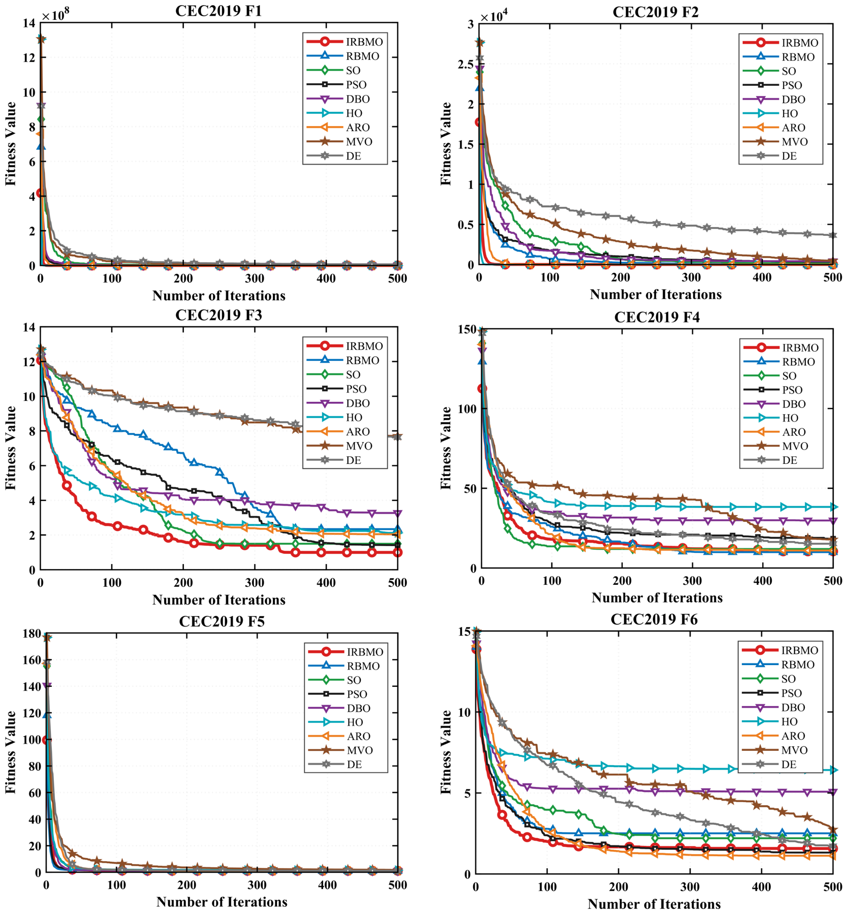
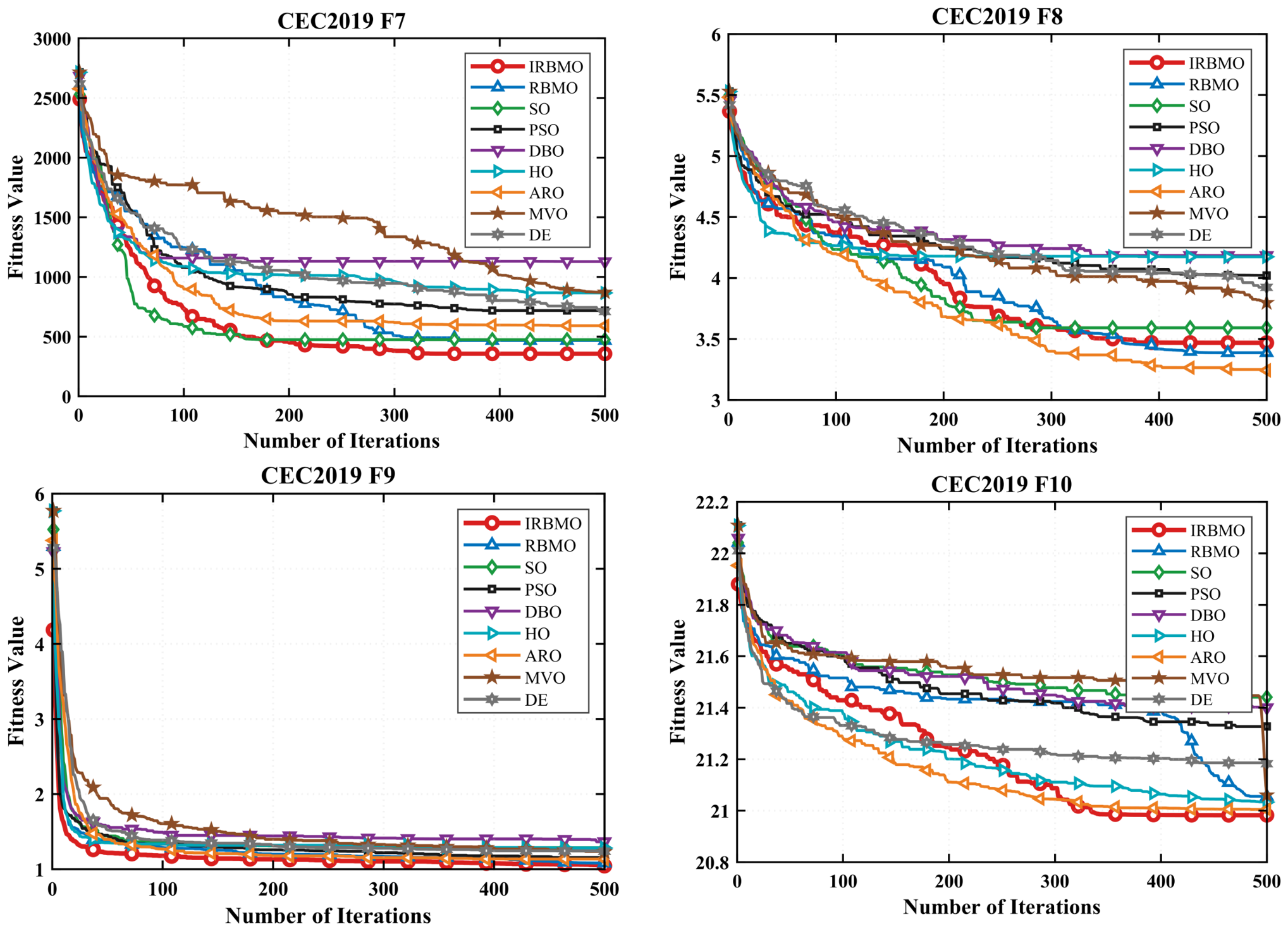
As shown in Table 2, IRBMO obtains the best mean values on seven of the ten benchmark functions and outperforms most competing algorithms overall. The median convergence curves in Figure 3 show that IRBMO converges relatively quickly and achieves high final solution accuracy on F1, F2, F3, F4, F7, F9, and F10. For several complex functions, the solution quality continues to improve during the middle and late iterations, indicating that IRBMO maintains its global search capability throughout the optimization process.

IRBMO also obtains relatively small standard deviations on several functions, indicating stable optimization performance. Although larger fluctuations occur on a few functions, its mean solution quality remains competitive. Overall, the statistical results show that the proposed strategies improve the solution accuracy and overall optimization performance of IRBMO.

On most functions, the convergence curves of IRBMO decrease rapidly during the early stage. This suggests that the composite chaotic initialization strategy improves the initial population and accelerates early convergence. During subsequent iterations, the anti-predation mechanism and multi-stage fine foraging strategy help the algorithm escape local optima and continue searching for better solutions. On F10 in particular, IRBMO overcomes the stagnation encountered by most comparison algorithms. This convergence behavior is consistent with the statistical results in Table 2.

Overall, the statistical results and convergence curves show that IRBMO performs competitively on the CEC2019 benchmark suite. The results support the effectiveness of the proposed improvement strategies and the application of IRBMO to complex engineering optimization problems.

4.3. Statistical Analysis

Because metaheuristic algorithms are stochastic, mean objective-function values and the best solutions obtained alone may not provide a reliable assessment of algorithm performance. The Wilcoxon signed-rank test and Friedman rank test are therefore used to evaluate the performance and robustness of IRBMO.

4.3.1. Wilcoxon Signed-Rank Test

The Wilcoxon signed-rank test is used to determine whether the performance difference between IRBMO and each comparison algorithm is statistically significant. For each benchmark function, the objective-function values obtained over 30 runs are paired using the same run indices. The significance level is set to $\alpha =0.05$; a p-value below 0.05 indicates a statistically significant difference between the two algorithms.

Table 3. Wilcoxon signed-rank test results.

Comparison	+	=	−
IRBMO vs. RBMO	7	3	0
IRBMO vs. SO	10	0	0
IRBMO vs. PSO	9	1	0
IRBMO vs. DBO	10	0	0
IRBMO vs. HO	9	1	0
IRBMO vs. ARO	6	3	1
IRBMO vs. MVO	10	0	0
IRBMO vs. DE	9	1	0
Total	70	9	1

summarizes the Wilcoxon signed-rank test results for IRBMO and the comparison algorithms on the ten CEC2019 benchmark functions. In the table, “+” indicates that IRBMO performs significantly better than the comparison algorithm, “=” indicates no statistically significant difference, and “−” indicates significantly worse performance.

As shown in Table 3, IRBMO records 70 significant wins, nine nonsignificant differences, and one significant loss across the 80 function-level comparisons. It significantly outperforms SO, DBO, and MVO on all ten benchmark functions and achieves nine significant wins against each of PSO, HO, and DE. IRBMO also shows some improvement over RBMO and ARO. Under the adopted exploratory setting, these results indicate that IRBMO generally performs well across the CEC2019 benchmark suite.

4.3.2. Friedman Test

The Friedman rank test is used to compare the overall performance of the algorithms on the ten CEC2019 benchmark functions. For each function, the algorithms are ranked according to the mean final objective-function values obtained over 30 runs. A smaller mean value corresponds to a better rank, and tied algorithms are assigned average ranks.

Table 4. Friedman rank test results.

Algorithm	Mean Rank	Overall Order
IRBMO	1.45	1
ARO	2.40	2
RBMO	3.30	3
SO	5.10	4
PSO	5.60	5
HO	6.25	6
DE	6.30	7
MVO	6.70	8
DBO	7.90	9

summarizes the mean ranks and overall rankings.

As shown in Table 4, IRBMO has the lowest mean rank of 1.45 and ranks first overall. Its consistently high rankings across most benchmark functions indicate that the overall advantage is not limited to a small subset of functions. These results demonstrate its overall optimization capability and adaptability to different problem characteristics. The Friedman omnibus test yields $Q=49.5667$, $df=8$, and $p=4.9500\times {10}^{-8}<0.05$. This result shows that the rank distributions of the nine algorithms are not identical and that at least one algorithm differs significantly from the others. Therefore, the overall ranking differences are unlikely to result entirely from random variation.

4.3.3. Parameter Sensitivity Analysis

The optimization performance of IRBMO is affected by the step-size coefficient P and the stage-transition parameters $(T_1,T_2)$. Specifically, P regulates the position-update step size in the multi-stage fine foraging strategy, while $T_1$ and $T_2$ determine the transitions from the early to the middle stage and from the middle to the late stage, respectively. To evaluate the rationality of the parameter settings, sensitivity experiments were conducted on the CEC2019 benchmark functions F1–F10, using the mean, standard deviation, and average rank of the final fitness values as evaluation metrics.

For parameter P, six candidate values—namely, $0.1$, $0.3$, $0.5$, $0.7$, $1.0$, and $1.5$—were examined. The results are presented in

Table 5. Results of sensitivity analysis for parameter P.

Function	Statistic	$\mathit{P}=0.1$	$\mathit{P}=0.3$	$\mathit{P}=0.5$	$\mathit{P}=0.7$	$\mathit{P}=1.0$	$\mathit{P}=1.5$
F1	Mean	$1.0003\times {10}^0$	$1.0000\times {10}^0$	$1.0000\times {10}^0$	$1.0000\times {10}^0$	$1.0001\times {10}^0$	$1.0000\times {10}^0$
	Std	$1.8921\times {10}^{-3}$	$1.8956\times {10}^{-4}$	$0.0000\times {10}^0$	$5.1197\times {10}^{-5}$	$3.1487\times {10}^{-4}$	$2.1819\times {10}^{-4}$
F2	Mean	$3.4443\times {10}^0$	$3.1844\times {10}^0$	$2.9550\times {10}^0$	$3.4116\times {10}^0$	$3.1160\times {10}^0$	$3.3940\times {10}^0$
	Std	$6.6776\times {10}^{-1}$	$5.3258\times {10}^{-1}$	$2.7535\times {10}^{-1}$	$7.8189\times {10}^{-1}$	$4.0637\times {10}^{-1}$	$6.3049\times {10}^{-1}$
F3	Mean	$1.3546\times {10}^0$	$1.2864\times {10}^0$	$1.2046\times {10}^0$	$1.3000\times {10}^0$	$1.3137\times {10}^0$	$1.3563\times {10}^0$
	Std	$1.4146\times {10}^{-1}$	$1.9069\times {10}^{-1}$	$2.0806\times {10}^{-1}$	$1.8402\times {10}^{-1}$	$1.7600\times {10}^{-1}$	$1.4242\times {10}^{-1}$
F4	Mean	$1.3669\times {10}^1$	$1.5361\times {10}^1$	$1.0253\times {10}^1$	$1.3072\times {10}^1$	$1.3868\times {10}^1$	$9.2913\times {10}^0$
	Std	$5.9234\times {10}^0$	$7.4303\times {10}^0$	$2.9231\times {10}^0$	$5.4291\times {10}^0$	$5.4867\times {10}^0$	$2.1913\times {10}^0$
F5	Mean	$1.1237\times {10}^0$	$1.1129\times {10}^0$	$1.0810\times {10}^0$	$1.0982\times {10}^0$	$1.0926\times {10}^0$	$1.1115\times {10}^0$
	Std	$4.6826\times {10}^{-2}$	$6.4334\times {10}^{-2}$	$2.8866\times {10}^{-2}$	$4.9565\times {10}^{-2}$	$4.8601\times {10}^{-2}$	$5.9607\times {10}^{-2}$
F6	Mean	$2.5162\times {10}^0$	$2.6534\times {10}^0$	$1.5994\times {10}^0$	$2.7222\times {10}^0$	$2.0787\times {10}^0$	$2.2024\times {10}^0$
	Std	$1.1960\times {10}^0$	$1.2446\times {10}^0$	$4.1582\times {10}^{-1}$	$1.1826\times {10}^0$	$1.0257\times {10}^0$	$9.8369\times {10}^{-1}$
F7	Mean	$5.5422\times {10}^2$	$4.4225\times {10}^2$	$3.3501\times {10}^2$	$4.3170\times {10}^2$	$4.9044\times {10}^2$	$4.3875\times {10}^2$
	Std	$1.8123\times {10}^2$	$1.8144\times {10}^2$	$1.1425\times {10}^2$	$1.5880\times {10}^2$	$1.6279\times {10}^2$	$1.4201\times {10}^2$
F8	Mean	$3.6801\times {10}^0$	$3.8539\times {10}^0$	$3.3216\times {10}^0$	$3.6087\times {10}^0$	$3.6202\times {10}^0$	$3.1450\times {10}^0$
	Std	$4.3567\times {10}^{-1}$	$4.3458\times {10}^{-1}$	$3.3036\times {10}^{-1}$	$3.9061\times {10}^{-1}$	$4.4362\times {10}^{-1}$	$4.6668\times {10}^{-1}$
F9	Mean	$1.0696\times {10}^0$	$1.0619\times {10}^0$	$1.0475\times {10}^0$	$1.0559\times {10}^0$	$1.0662\times {10}^0$	$1.0585\times {10}^0$
	Std	$2.2661\times {10}^{-2}$	$2.2173\times {10}^{-2}$	$1.3011\times {10}^{-2}$	$2.4884\times {10}^{-2}$	$2.5618\times {10}^{-2}$	$2.6793\times {10}^{-2}$
F10	Mean	$1.7002\times {10}^1$	$1.8402\times {10}^1$	$1.6415\times {10}^1$	$1.7658\times {10}^1$	$1.5770\times {10}^1$	$1.9007\times {10}^1$
	Std	$8.1379\times {10}^0$	$6.7152\times {10}^0$	$8.4376\times {10}^0$	$7.5773\times {10}^0$	$8.8240\times {10}^0$	$6.1051\times {10}^0$
Average rank		5.10	4.30	1.30	3.30	3.50	3.50

. Among the six settings, $P=0.5$ obtains the lowest average rank of 1.30 and achieves the smallest mean fitness value on F1, F2, F3, F5, F6, F7, and F9. Although $P=1.5$ performs better on F4 and F8, and $P=1.0$ obtains the best result on F10, neither setting maintains its advantage over the complete benchmark set. A small value of P restricts the position-update step and may weaken the global search capability, whereas an excessively large value introduces stronger perturbations and may reduce the accuracy of local refinement. Therefore, $P=0.5$ provides the best overall performance and is adopted in the subsequent experiments.

The sensitivity of the stage-transition parameters was examined using six combinations: $(0.20,0.50)$, $(0.20,0.80)$, $(0.33,0.67)$, $(0.33,0.80)$, $(0.40,0.60)$, and $(0.50,0.80)$. The results are reported in

Table 6. Results of sensitivity analysis for parameters $T_1$ and $T_2$.

Function	Statistic	$(0.20,0.50)$	$(0.20,0.80)$	$(0.33,0.67)$	$(0.33,0.80)$	$(0.40,0.60)$	$(0.50,0.80)$
F1	Mean	$1.0000\times {10}^0$	$1.0000\times {10}^0$	$1.0000\times {10}^0$	$1.0000\times {10}^0$	$1.0000\times {10}^0$	$1.0000\times {10}^0$
	Std	$1.4807\times {10}^{-4}$	$1.1535\times {10}^{-14}$	$1.0909\times {10}^{-16}$	$1.8429\times {10}^{-14}$	$2.5777\times {10}^{-4}$	$1.4926\times {10}^{-14}$
F2	Mean	$3.5705\times {10}^0$	$3.0256\times {10}^0$	$2.8146\times {10}^0$	$3.1867\times {10}^0$	$3.0708\times {10}^0$	$3.2134\times {10}^0$
	Std	$7.1235\times {10}^{-1}$	$5.9135\times {10}^{-1}$	$4.6529\times {10}^{-1}$	$5.3236\times {10}^{-1}$	$6.3062\times {10}^{-1}$	$4.9947\times {10}^{-1}$
F3	Mean	$1.3000\times {10}^0$	$1.2318\times {10}^0$	$1.1227\times {10}^0$	$1.1909\times {10}^0$	$1.2591\times {10}^0$	$1.2455\times {10}^0$
	Std	$1.8402\times {10}^{-1}$	$2.0621\times {10}^{-1}$	$1.9069\times {10}^{-1}$	$2.0760\times {10}^{-1}$	$2.0053\times {10}^{-1}$	$2.0386\times {10}^{-1}$
F4	Mean	$1.3935\times {10}^1$	$1.1149\times {10}^1$	$9.5567\times {10}^0$	$1.1381\times {10}^1$	$1.4432\times {10}^1$	$1.3043\times {10}^1$
	Std	$4.8742\times {10}^0$	$4.4597\times {10}^0$	$2.7849\times {10}^0$	$4.1210\times {10}^0$	$5.9454\times {10}^0$	$5.1932\times {10}^0$
F5	Mean	$1.1292\times {10}^0$	$1.1001\times {10}^0$	$1.0885\times {10}^0$	$1.1152\times {10}^0$	$1.1252\times {10}^0$	$1.0944\times {10}^0$
	Std	$5.9710\times {10}^{-2}$	$4.5328\times {10}^{-2}$	$3.2596\times {10}^{-2}$	$6.2959\times {10}^{-2}$	$6.4931\times {10}^{-2}$	$5.9878\times {10}^{-2}$
F6	Mean	$2.3234\times {10}^0$	$2.3126\times {10}^0$	$1.5172\times {10}^0$	$2.8584\times {10}^0$	$2.1704\times {10}^0$	$2.6840\times {10}^0$
	Std	$1.0580\times {10}^0$	$1.0581\times {10}^0$	$3.9344\times {10}^{-1}$	$1.2621\times {10}^0$	$8.5677\times {10}^{-1}$	$9.4295\times {10}^{-1}$
F7	Mean	$5.3562\times {10}^2$	$4.1130\times {10}^2$	$4.2203\times {10}^2$	$4.6209\times {10}^2$	$4.1404\times {10}^2$	$5.3590\times {10}^2$
	Std	$1.9222\times {10}^2$	$1.6357\times {10}^2$	$1.0630\times {10}^2$	$1.3370\times {10}^2$	$1.3923\times {10}^2$	$1.8251\times {10}^2$
F8	Mean	$3.6345\times {10}^0$	$3.5050\times {10}^0$	$3.3975\times {10}^0$	$3.8655\times {10}^0$	$3.7238\times {10}^0$	$3.6962\times {10}^0$
	Std	$5.0826\times {10}^{-1}$	$5.9741\times {10}^{-1}$	$2.7021\times {10}^{-1}$	$5.2408\times {10}^{-1}$	$4.1476\times {10}^{-1}$	$4.0953\times {10}^{-1}$
F9	Mean	$1.0657\times {10}^0$	$1.0600\times {10}^0$	$1.0509\times {10}^0$	$1.0688\times {10}^0$	$1.0642\times {10}^0$	$1.0653\times {10}^0$
	Std	$2.2130\times {10}^{-2}$	$2.2137\times {10}^{-2}$	$1.1713\times {10}^{-2}$	$2.3657\times {10}^{-2}$	$2.3783\times {10}^{-2}$	$1.7768\times {10}^{-2}$
F10	Mean	$1.9700\times {10}^1$	$1.8329\times {10}^1$	$1.5693\times {10}^1$	$1.7712\times {10}^1$	$1.8422\times {10}^1$	$1.7743\times {10}^1$
	Std	$4.9286\times {10}^0$	$6.9116\times {10}^0$	$8.9256\times {10}^0$	$7.4569\times {10}^0$	$6.6764\times {10}^0$	$7.3671\times {10}^0$
Average rank		5.10	2.40	1.20	4.10	4.20	4.00

. The combination $(T_1,T_2)=(0.33,0.67)$ obtains the smallest mean fitness value on nine of the ten benchmark functions and achieves the best overall average rank. The only exception is F7, on which $(0.20,0.80)$ produces a slightly lower mean value. Moreover, $(0.33,0.67)$ yields relatively small standard deviations on most functions, indicating stable performance across repeated runs. These results show that allocating approximately one third of the iterations to each search stage provides a suitable balance among global exploration, transitional search, and local exploitation. Consequently, $(T_1,T_2)=(0.33,0.67)$ is adopted as the stage-transition setting of IRBMO.

4.3.4. Ablation Study

To quantify the contribution of each improvement strategy, four single-strategy variants were constructed using RBMO as the baseline. ${\mathrm{IRBMO}}_1$, ${\mathrm{IRBMO}}_2$, ${\mathrm{IRBMO}}_3$, and ${\mathrm{IRBMO}}_4$ incorporate only the composite chaotic mapping, anti-predation strategy, multi-stage fine foraging strategy, and simulated annealing mechanism, respectively. RBMO and IRBMO were also included in the comparison. The ablation results are reported in

Table 7. Results of the ablation study.

Function	Statistic	RBMO	${\mathbf{IRBMO}}_1$	${\mathbf{IRBMO}}_2$	${\mathbf{IRBMO}}_3$	${\mathbf{IRBMO}}_4$	IRBMO
F1	Mean	$1.0255\times {10}^0$	$1.0307\times {10}^0$	$1.0004\times {10}^0$	$1.0005\times {10}^0$	$1.0483\times {10}^0$	$1.0000\times {10}^0$
	Std	$3.0111\times {10}^{-2}$	$4.3980\times {10}^{-2}$	$1.7076\times {10}^{-3}$	$1.4551\times {10}^{-3}$	$6.1663\times {10}^{-2}$	$1.3910\times {10}^{-15}$
F2	Mean	$1.0132\times {10}^1$	$1.0018\times {10}^1$	$3.9323\times {10}^0$	$3.7646\times {10}^0$	$1.3266\times {10}^1$	$2.9045\times {10}^0$
	Std	$7.3225\times {10}^0$	$5.0952\times {10}^0$	$7.6784\times {10}^{-1}$	$1.7552\times {10}^0$	$5.9659\times {10}^0$	$3.6256\times {10}^{-1}$
F3	Mean	$3.5485\times {10}^0$	$3.8089\times {10}^0$	$1.4304\times {10}^0$	$1.3979\times {10}^0$	$7.9652\times {10}^0$	$1.2597\times {10}^0$
	Std	$1.6625\times {10}^0$	$1.9433\times {10}^0$	$2.1147\times {10}^{-1}$	$1.3917\times {10}^{-1}$	$2.3754\times {10}^0$	$2.0053\times {10}^{-1}$
F4	Mean	$1.1900\times {10}^1$	$1.1256\times {10}^1$	$7.1356\times {10}^0$	$1.5612\times {10}^1$	$1.2815\times {10}^1$	$1.1812\times {10}^1$
	Std	$3.9871\times {10}^0$	$3.7160\times {10}^0$	$2.3528\times {10}^0$	$5.6687\times {10}^0$	$5.0057\times {10}^0$	$2.8351\times {10}^0$
F5	Mean	$1.0621\times {10}^0$	$1.0797\times {10}^0$	$1.0944\times {10}^0$	$1.0722\times {10}^0$	$1.1647\times {10}^0$	$1.0985\times {10}^0$
	Std	$3.5548\times {10}^{-2}$	$5.1639\times {10}^{-2}$	$4.6130\times {10}^{-2}$	$4.3098\times {10}^{-2}$	$7.5243\times {10}^{-2}$	$2.9444\times {10}^{-2}$
F6	Mean	$1.9078\times {10}^0$	$2.8953\times {10}^0$	$2.0134\times {10}^0$	$2.1274\times {10}^0$	$3.2159\times {10}^0$	$1.8425\times {10}^0$
	Std	$1.2613\times {10}^0$	$1.4050\times {10}^0$	$1.3409\times {10}^0$	$6.9139\times {10}^{-1}$	$1.6369\times {10}^0$	$5.9801\times {10}^{-1}$
F7	Mean	$4.8223\times {10}^2$	$4.8170\times {10}^2$	$3.5710\times {10}^2$	$5.4272\times {10}^2$	$5.4582\times {10}^2$	$3.7731\times {10}^2$
	Std	$2.3339\times {10}^2$	$2.3093\times {10}^2$	$1.9137\times {10}^2$	$2.0299\times {10}^2$	$2.9840\times {10}^2$	$1.0111\times {10}^2$
F8	Mean	$3.3698\times {10}^0$	$3.4267\times {10}^0$	$2.9802\times {10}^0$	$3.6497\times {10}^0$	$3.9621\times {10}^0$	$3.4688\times {10}^0$
	Std	$3.5788\times {10}^{-1}$	$3.2972\times {10}^{-1}$	$5.2994\times {10}^{-1}$	$3.7624\times {10}^{-1}$	$5.2882\times {10}^{-1}$	$4.0076\times {10}^{-1}$
F9	Mean	$1.0865\times {10}^0$	$1.0803\times {10}^0$	$1.0577\times {10}^0$	$1.0934\times {10}^0$	$1.0634\times {10}^0$	$1.0551\times {10}^0$
	Std	$5.6252\times {10}^{-2}$	$3.3111\times {10}^{-2}$	$1.8638\times {10}^{-2}$	$3.2903\times {10}^{-2}$	$2.4181\times {10}^{-2}$	$1.5350\times {10}^{-2}$
F10	Mean	$2.0868\times {10}^1$	$2.1035\times {10}^1$	$1.8063\times {10}^1$	$1.7136\times {10}^1$	$2.1094\times {10}^1$	$1.6360\times {10}^1$
	Std	$9.9220\times {10}^{-1}$	$3.9579\times {10}^{-2}$	$6.7212\times {10}^0$	$7.1612\times {10}^0$	$8.3812\times {10}^{-2}$	$8.5258\times {10}^0$
Average rank		3.50	3.90	2.30	3.70	5.60	2.00
Average running time t (s)		0.7917	0.7917	0.9990	2.3373	0.7887	2.5553

.

IRBMO attains the lowest average rank of 2.00, followed by ${\mathrm{IRBMO}}_2$ with 2.30 and RBMO with 3.50. It also produces the lowest mean fitness values on F1, F2, F3, F6, F9, and F10, indicating consistent performance across the benchmark set. In addition, IRBMO records the smallest standard deviations on F1, F2, F5, F6, F7, and F9, showing good stability over independent runs.

The lower average rank of IRBMO than those of all the single-strategy variants suggests that the four strategies are most effective when used together. Each strategy has a distinct and complementary function in the optimization process. The composite chaotic mapping improves the initial population distribution, while the anti-predation strategy maintains population diversity. The multi-stage fine foraging strategy adjusts the search behavior across the optimization stages, and the simulated annealing mechanism applies a probabilistic acceptance criterion when updating candidate solutions. Together, these strategies preserve population diversity during global exploration and strengthen local exploitation as the search progresses, providing a better balance between solution accuracy and optimization stability on the CEC2019 benchmark functions.

The performance gain is accompanied by a higher computational cost. The average runtime increases from 0.7917 s per run for RBMO to 2.5553 s for IRBMO. This increase mainly results from the introduction of the multi-stage fine foraging strategy. Thus, IRBMO improves solution accuracy and stability at the cost of a longer runtime, reflecting the trade-off between optimization performance and computational efficiency.

5. Case Study

5.1. Experimental Data

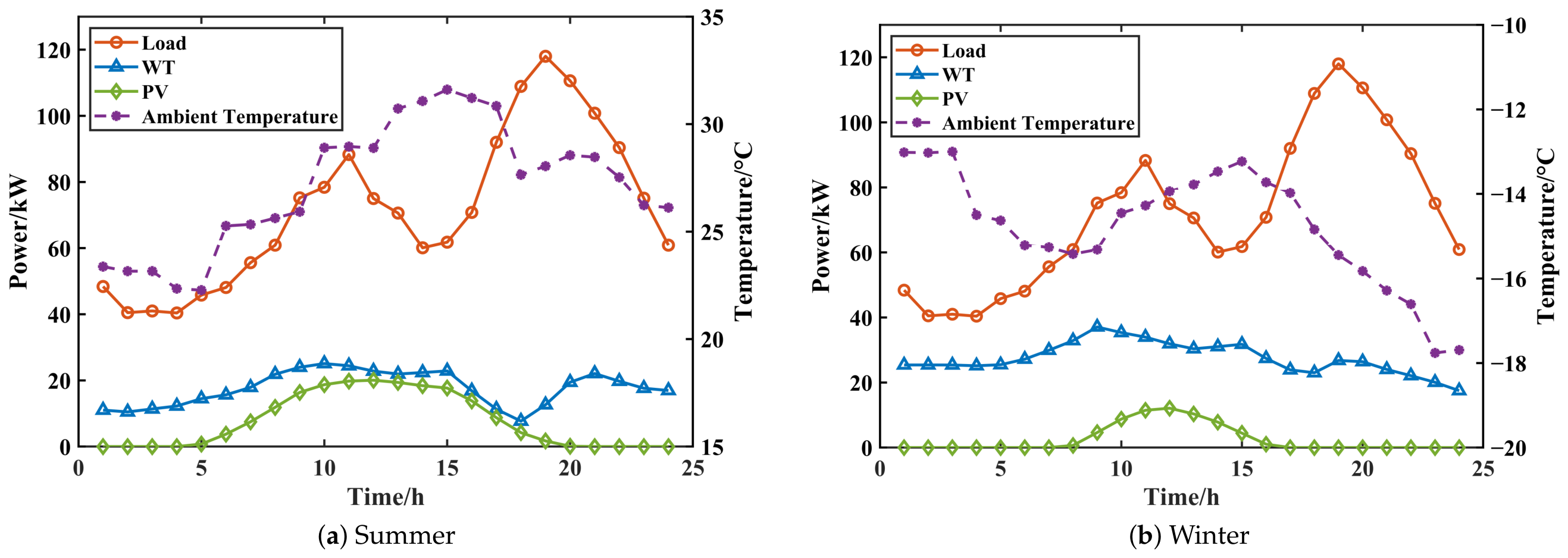
To validate the performance of the formulated model and the optimization algorithm, a specific locale in Northeast China is chosen for empirical analysis. Endowed with abundant wind and solar resources as well as a solid industrial foundation, this region serves as a pivotal area for conducting research on clean energy integration and regional energy system optimization. Figure 4 illustrates the wind and solar power outputs, electrical loads, and temperature data for typical days in summer and winter within this region.

To incentivize users to optimize their consumption schedules and maintain a robust supply–demand balance, a time-of-use pricing mechanism is implemented. This strategy determines electricity tariffs based on the system’s average marginal operational costs.

Table 8. Time-of-use electricity prices for interaction with the utility grid.

Mode	Time	Price (CNY/kWh)
Purchase electricity	Peak period (10:00–13:00, 17:00–20:00)	1.28
	Regular period (07:00–09:00, 14:00–16:00, 21:00–22:00)	0.72
	Valley period (01:00–06:00, 23:00–24:00)	0.34
Sell electricity	Peak period (10:00–13:00, 17:00–20:00)	1.12
	Regular period (07:00–09:00, 14:00–16:00, 21:00–22:00)	0.61
	Valley period (01:00–06:00, 23:00–24:00)	0.21

Note: CNY, Chinese yuan.

presents the time-of-use electricity prices in this region.

The pollutant treatment costs and the corresponding emission coefficients are presented in

Table 9. Pollutant treatment costs and related coefficients.

Type	Treatment Cost (CNY/kg)	Emission Coefficients of Pollutants (g/kWh)
		MT	FC	Main Grid
${\mathrm{CO}}_2$	0.21	724	489	889
${\mathrm{SO}}_2$	14.842	0.0036	0.0027	1.8
${\mathrm{NO}}_x$	62.964	0.2	0.014	1.6

Note: MT, microturbine; FC, fuel cell.

. The maintenance cost coefficients of the microgrid components are summarized in

Table 10. Maintenance cost coefficients of the microgrid components.

Component	Symbol	Maintenance Cost Coefficient (CNY/kWh)
PV	$K_{\mathrm{PV}}$	0.01
WT	$K_{\mathrm{WT}}$	0.298
MT	$K_{\mathrm{MT}}$	0.031
FC	$K_{\mathrm{FC}}$	0.087
SB	$K_{\mathrm{SB}}$	0.0012

Note: SB, storage battery.

, while their principal technical parameters and operating limits are provided in

Table 11. Principal parameter values and operating limits of the microgrid model.

Symbol	Value	Unit	Symbol	Value	Unit
$P_{\mathrm{STC}}$	30	kW	$G_{\mathrm{STC}}$	1000	$\mathrm{W}/{\mathrm{m}}^2$
k	$-0.0047$	${°\mathrm{C}}^{-1}$	$T_{\mathrm{ref}}$	25	$°\mathrm{C}$
$\mathrm{NOCT}$	45	$°\mathrm{C}$	$P_{\mathrm{r}}$	40	kW
$v_{\mathrm{ci}}/v_{\mathrm{r}}/v_{\mathrm{co}}$	$2.6/9.5/25$	m/s	$C_{\mathrm{ng}}$	2.99	$\mathrm{CNY}/{\mathrm{m}}^3$
$LH{V}_{\mathrm{ng}}$	9.7	$\mathrm{kWh}/{\mathrm{m}}^3$	$P_{\mathrm{grid},min}/P_{\mathrm{grid},max}$	$-20/20$	kW
$P_{\mathrm{SB},min}/P_{\mathrm{SB},max}$	$-20/20$	kW	$P_{\mathrm{c},max}/P_{\mathrm{dis},max}$	$20/20$	kW
${\mathrm{SOC}}_{min}/{\mathrm{SOC}}_{max}$	$0.2/0.9$	–	$E_{\mathrm{r}}$	100	kWh
$E_0$	50	kWh	${\eta }_{\mathrm{c}}/{\eta }_{\mathrm{dis}}$	$0.95/0.95$	–
$\mathrm{SOC}\left(0\right)$	0.5	–	$P_{\mathrm{MT},min}/P_{\mathrm{MT},max}$	$5/65$	kW
$P_{\mathrm{FC},min}/P_{\mathrm{FC},max}$	$5/50$	kW	$R_{\mathrm{MT}}^{\mathrm{up}}/R_{\mathrm{MT}}^{\mathrm{down}}$	$35/30$	kW/h
$R_{\mathrm{FC}}^{\mathrm{up}}/R_{\mathrm{FC}}^{\mathrm{down}}$	$25/20$	kW/h	–	–	–

.

5.2. Simulation Results Analysis

To evaluate the effectiveness of IRBMO in solving the optimal dispatch problem of the grid-connected microgrid, three representative scenarios are considered: Scenario 1 includes PV, WT, MT, FC, and SB; Scenario 2 includes WT, MT, FC, and SB; and Scenario 3 includes PV, MT, FC, and SB.

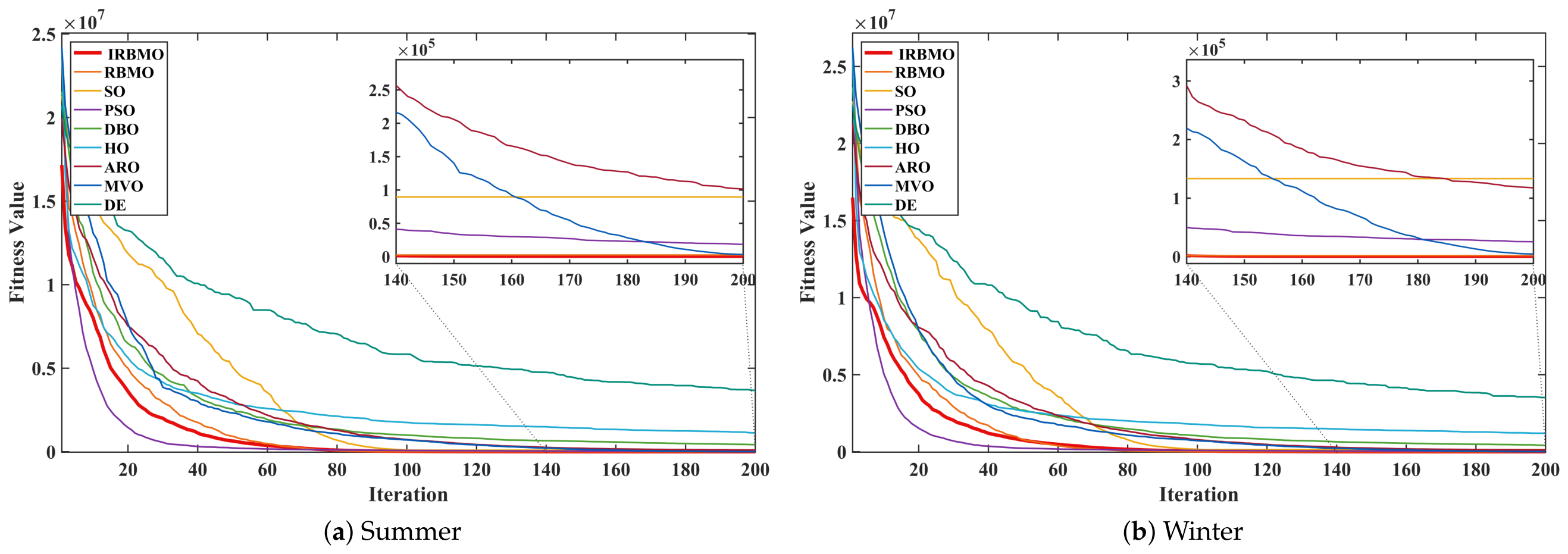
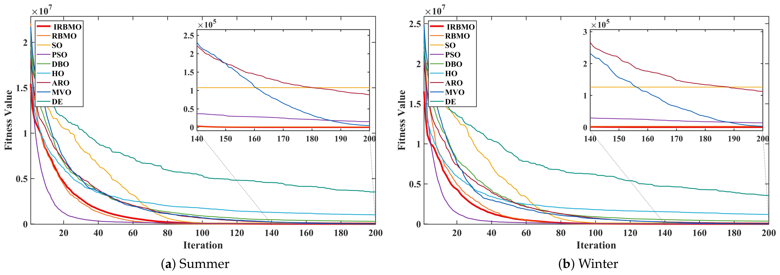
Comparative experiments are conducted using IRBMO and eight benchmark algorithms. The population size and maximum number of iterations are set to 50 and 200, respectively, for all scenarios. Each algorithm is independently run 20 times for each case, and the mean results are used to determine the final dispatch scheme.

5.2.1. Scenario 1: PV-WT-MT-FC-SB Microgrid

Scenario 1 is the base operating condition, with PV, WT, MT, FC, and SB all available. As shown in

Table 12. Simulation results of different algorithms in Scenario 1.

Season	Item	IRBMO	RBMO	PSO	SO	DBO	HO	ARO	MVO	DE
Summer	Mean (CNY)	1578.20	1613.33	1617.69	1619.98	1613.45	1600.59	1592.80	1585.67	1615.11
	Std	19.37	23.45	41.08	28.73	65.53	26.33	17.74	35.20	52.82
	Emissions (kg)	850.66	907.23	912.35	906.56	971.27	881.36	856.05	897.32	928.82
	Cost saving rate (%)	–	2.18	2.44	2.58	2.18	1.40	0.92	0.47	2.29
Winter	Mean (CNY)	1535.46	1581.06	1569.59	1593.22	1585.69	1572.30	1543.80	1561.30	1596.60
	Std	20.99	27.53	37.77	24.31	53.81	30.52	14.84	33.63	63.81
	Emissions (kg)	792.51	848.69	854.59	849.05	921.87	829.35	789.78	847.67	878.50
	Cost saving rate (%)	–	2.88	2.17	3.63	3.17	2.34	0.54	1.66	3.83

, IRBMO achieves the lowest mean comprehensive cost among the nine algorithms in both seasons. Its mean comprehensive costs are 1578.20 Chinese yuan (CNY) in summer and 1535.46 CNY in winter, with standard deviations of 19.37 and 20.99, respectively. These standard deviations are the second lowest among the compared algorithms, indicating stable performance across independent runs. The corresponding mean emissions are 850.66 kg and 792.51 kg. IRBMO records the lowest mean emissions in summer, while its winter value is slightly higher than the 789.78 kg obtained by ARO. Compared with the eight benchmark algorithms, IRBMO reduces the mean comprehensive cost by 0.47–2.58% in summer and 0.54–3.83% in winter.

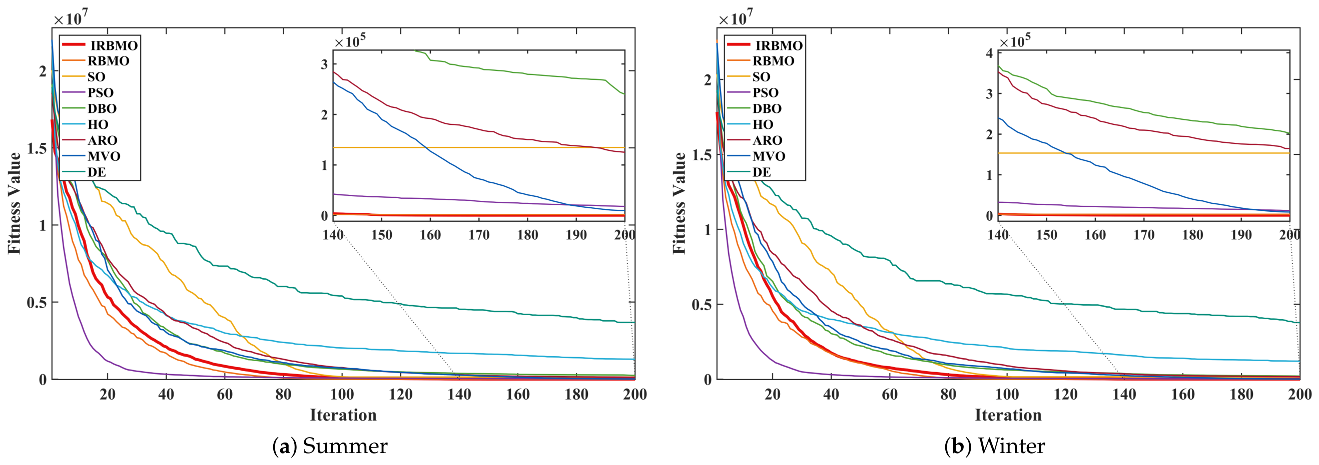
Figure 5 shows a rapid decrease in the IRBMO fitness value during the initial iterations, followed by convergence to a relatively low and stable level. This pattern indicates competitive convergence performance under the specified population size and maximum iteration limit of 200.

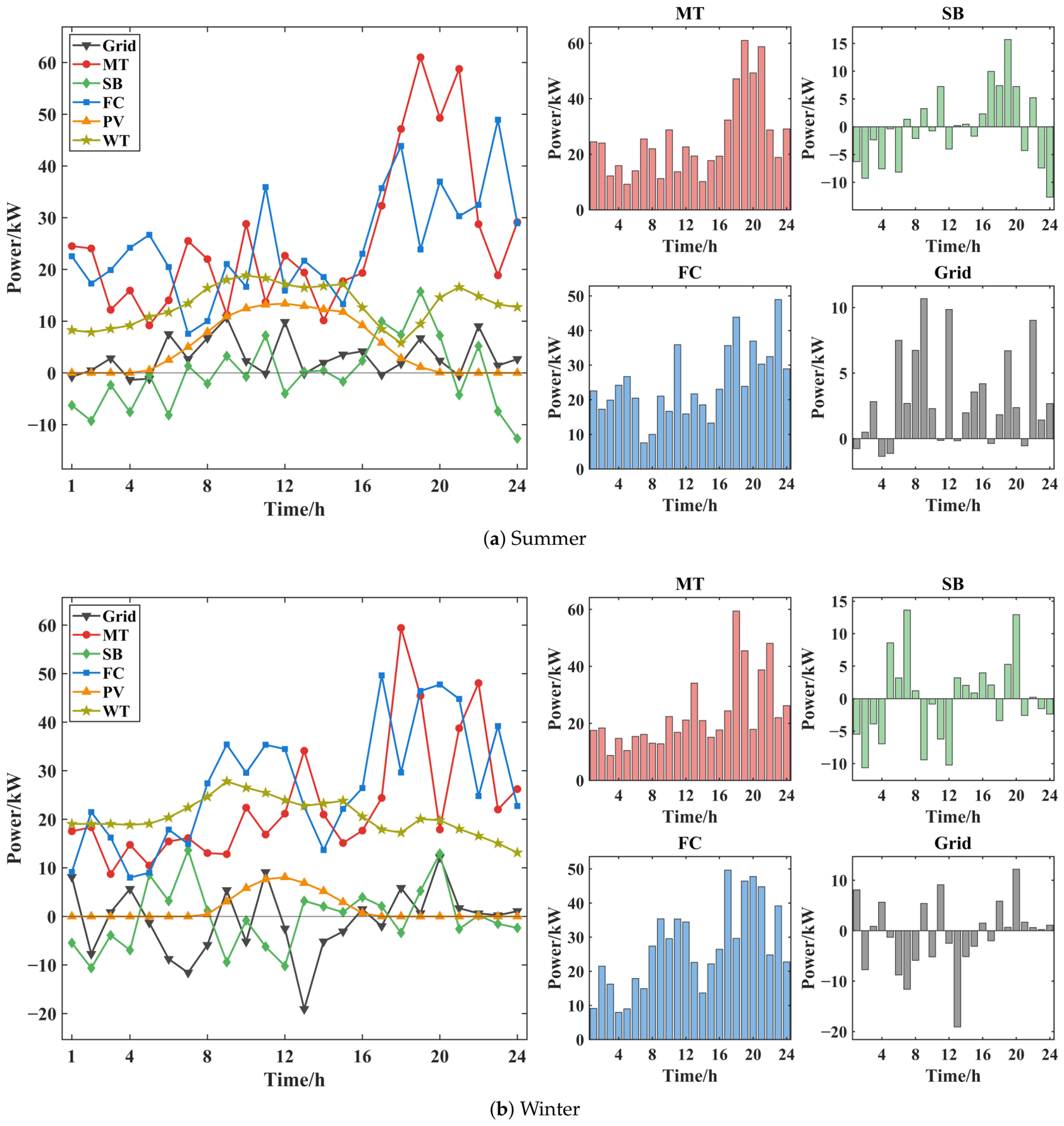
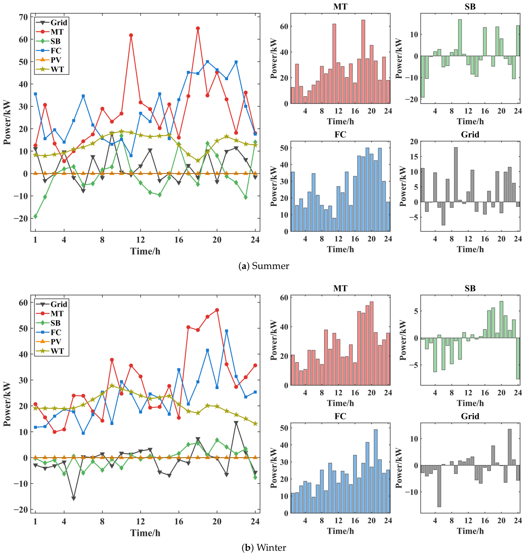
Figure 6 shows the dispatch schemes obtained by IRBMO for summer and winter. PV and WT directly supply the load when renewable generation is available, while MT, FC, SB, and the utility grid compensate for changes in renewable output and demand. In summer, PV supplies part of the daytime load, and MT and FC increase their outputs during several high-demand periods, particularly when PV generation declines. The lower winter PV output requires greater contributions from MT, FC, and the utility grid. SB alternates between charging and discharging over the scheduling horizon. It generally stores energy when electricity prices are relatively low or renewable generation is sufficient and releases energy during high-price or high-demand periods. This behavior shifts energy across time, reduces power supply pressure during peak-load periods, and supports the coordinated operation of the microgrid.

5.2.2. Scenario 2: WT-MT-FC-SB Microgrid

Scenario 2 represents the restricted operating condition without PV, while WT, MT, FC, and SB remain available.

Table 13. Simulation results of different algorithms in Scenario 2.

Season	Item	IRBMO	RBMO	PSO	SO	DBO	HO	ARO	MVO	DE
Summer	Mean (CNY)	1696.85	1719.33	1746.04	1730.97	1734.06	1714.58	1708.28	1703.92	1735.04
	Std	17.32	28.16	31.75	38.84	43.13	37.50	17.00	22.06	67.87
	Emissions (kg)	929.04	958.86	984.63	966.40	1045.50	946.78	931.60	980.10	1002.07
	Cost saving rate (%)	–	1.31	2.82	1.97	2.15	1.03	0.67	0.41	2.20
Winter	Mean (CNY)	1586.41	1627.42	1609.05	1619.84	1627.45	1603.49	1592.10	1615.05	1660.64
	Std	21.53	28.97	32.82	35.28	52.37	16.89	23.73	30.81	76.42
	Emissions (kg)	825.00	874.09	872.55	871.15	939.89	846.54	816.96	881.76	916.04
	Cost saving rate (%)	–	2.52	1.41	2.06	2.52	1.07	0.36	1.77	4.47

shows that IRBMO achieves the lowest mean comprehensive cost among the nine algorithms in both seasons, with values of 1696.85 CNY in summer and 1586.41 CNY in winter. The corresponding standard deviations are 17.32 and 21.53, both ranking second among the compared algorithms and indicating stable performance across independent runs. The mean emissions are 929.04 kg in summer and 825.00 kg in winter. IRBMO records the lowest mean emissions in summer, while its winter value is slightly higher than the 816.96 kg obtained by ARO. Compared with the eight benchmark algorithms, IRBMO reduces the mean comprehensive cost by 0.41–2.82% in summer and 0.36–4.47% in winter.

Figure 7 shows that the IRBMO fitness value decreases rapidly during the initial iterations and then converges to a relatively low and stable level. This pattern indicates competitive convergence performance under the specified population size and maximum iteration limit of 200.

Figure 8 shows the dispatch schemes obtained by IRBMO for summer and winter without PV generation. WT supplies renewable power throughout the scheduling horizon, while MT and FC adjust their outputs in response to changes in wind generation and load demand. Their outputs increase during several high-demand periods, particularly in the evening. The utility grid supplies the remaining deficit or absorbs surplus power according to the balance between generation and demand.

The SB power profile reflects the absence of surplus photovoltaic energy for daytime charging. In summer, SB frequently switches between charging and discharging to respond to changes in WT generation and load demand. In winter, it mainly charges during the first half of the scheduling horizon and discharges during several high-load periods in the evening and at night. Charging at the end of the scheduling horizon also satisfies the terminal SOC constraint. Without PV generation, SB transfers energy across time, partly compensates for the loss of daytime photovoltaic power, and reduces the power supply burden on MT, FC, and the utility grid during high-load periods.

5.2.3. Scenario 3: PV-MT-FC-SB Microgrid

Scenario 3 represents the restricted operating condition without WT, while PV, MT, FC, and SB remain available. As shown in

Table 14. Simulation results of different algorithms in Scenario 3.

Season	Item	IRBMO	RBMO	PSO	SO	DBO	HO	ARO	MVO	DE
Summer	Mean (CNY)	1795.06	1815.65	1817.32	1816.49	1839.09	1806.59	1793.66	1818.80	1825.26
	Std	19.68	29.50	26.34	32.73	47.57	26.85	21.25	36.77	70.54
	Emissions (kg)	1059.09	1083.05	1093.10	1086.62	1161.61	1076.62	1053.66	1106.41	1115.06
	Cost saving rate (%)	–	1.13	1.22	1.18	2.39	0.64	$-0.08$	1.31	1.65
Winter	Mean (CNY)	1875.62	1892.93	1905.67	1890.22	1911.06	1887.17	1878.79	1896.33	1877.59
	Std	17.25	17.02	31.93	36.26	59.61	30.44	20.26	29.94	77.39
	Emissions (kg)	1113.91	1131.72	1150.08	1132.03	1200.58	1131.46	1107.01	1156.54	1137.47
	Cost saving rate (%)	–	0.91	1.58	0.77	1.85	0.61	0.17	1.09	0.10

, IRBMO obtains mean comprehensive costs of 1795.06 CNY in summer and 1875.62 CNY in winter. In summer, ARO achieves the lowest value of 1793.66 CNY, which is 1.40 CNY lower than the IRBMO result. IRBMO nevertheless records the lowest standard deviation of 19.68. In winter, IRBMO achieves the lowest mean comprehensive cost of 1875.62 CNY, with a standard deviation of 17.25. Its mean emissions are 1059.09 kg in summer and 1113.91 kg in winter. ARO records the lowest mean emissions in both seasons, while IRBMO ranks second. Compared with seven of the eight benchmark algorithms, IRBMO reduces the summer mean comprehensive cost by 0.64–2.39%, but its cost is 0.08% higher than that obtained by ARO. In winter, IRBMO reduces the mean comprehensive cost by 0.10–1.85% relative to all eight benchmark algorithms.

Figure 9 shows that the IRBMO fitness value decreases rapidly during the initial iterations and then converges to a relatively low and stable level. This pattern indicates competitive convergence performance under the specified population size and maximum iteration limit of 200, even without WT generation.

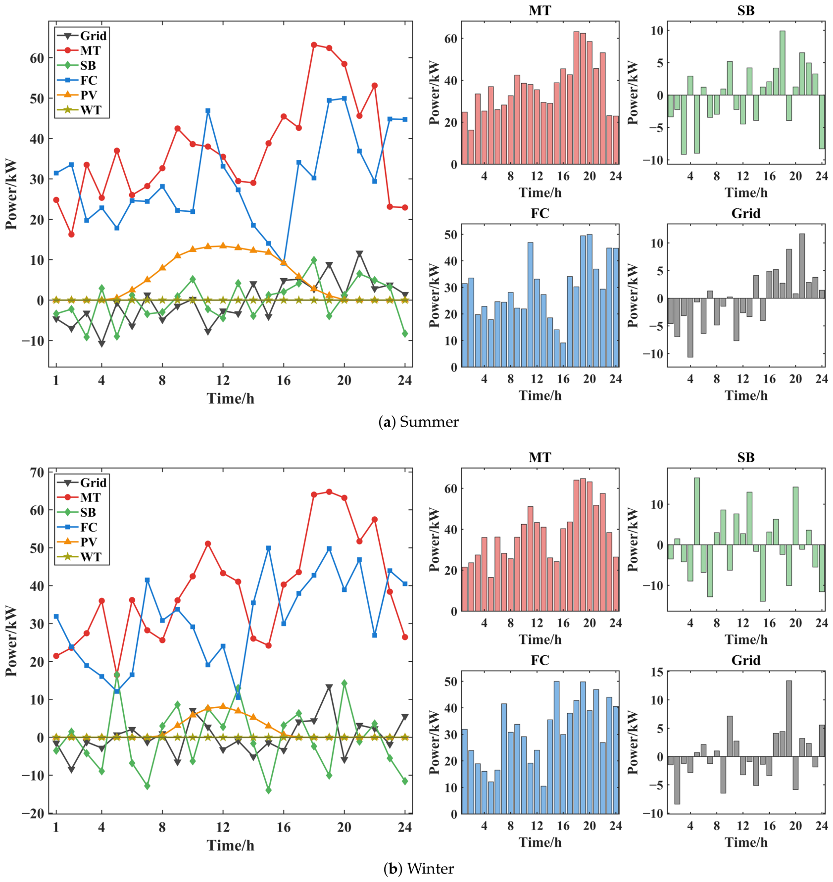
Figure 10 shows the dispatch schemes obtained by IRBMO for summer and winter without WT generation. PV generates power only during daylight hours and reaches its maximum output around midday. Without the continuous contribution of WT, MT and FC supply a substantial share of the load throughout the scheduling horizon and generally increase their outputs during evening high-demand periods as PV generation declines. The utility grid responds to changes in PV generation and load demand by supplying the remaining deficit or absorbing surplus power.

The SB power profile also reflects the absence of WT. Because surplus wind energy is unavailable for charging, SB operation depends mainly on daytime PV generation, time-of-use electricity prices, and load demand. In summer, SB generally charges during several early low-demand periods and discharges during selected daytime and evening periods. In winter, it switches more frequently between charging and discharging in response to changes in PV generation and demand. SB therefore transfers energy across time, partly compensates for the loss of continuous wind power, and reduces the power supply burden on MT, FC, and the utility grid during high-demand periods.

5.3. Comparative Analysis of Dispatch Results Under Three Scenarios

Table 12, Table 13 and Table 14 compare the comprehensive costs, standard deviations, emissions, and cost saving rates of the nine algorithms. IRBMO achieves the lowest mean comprehensive cost in five of the six operating cases. The exception is Scenario 3 in summer, where ARO obtains 1793.66 CNY, 1.40 CNY less than the 1795.06 CNY obtained by IRBMO. IRBMO also records relatively small standard deviations across the six cases, indicating stable performance over independent runs, and its mean emissions rank first or second in every case. Overall, IRBMO provides competitive comprehensive cost performance and optimization stability.

A comparison of the three scenarios shows how renewable-energy availability affects microgrid operation. Relative to Scenario 1, removing PV in Scenario 2 increases the IRBMO mean comprehensive cost by 7.52% in summer and 3.32% in winter; the corresponding mean emissions increase by 9.21% and 4.10%. Removing WT in Scenario 3 increases the mean comprehensive cost by 13.74% in summer and 22.15% in winter, while mean emissions rise by 24.50% and 40.55%. The simultaneous availability of PV and WT therefore produces lower comprehensive costs and emissions under the profiles considered. The larger increases observed without WT also indicate that WT provides more continuous renewable power support than PV in these cases.

Table 15. Average computational time of different algorithms.

Algorithm	IRBMO	RBMO	PSO	SO	DBO	HO	ARO	MVO	DE
Mean Runtime (s)	5.246	2.743	1.227	1.282	1.282	6.026	1.300	1.353	1.381

reports the average runtime of each algorithm across the six operating cases. IRBMO requires 5.246 s on average, less than the 6.026 s required by HO but more than the runtimes of the other benchmark algorithms. The additional computational cost arises from the introduction of multiple improvement mechanisms.

As shown in

Table 16. Friedman test results.

Algorithm	IRBMO	RBMO	PSO	SO	DBO	HO	ARO	MVO	DE
Mean Rank	3.108	5.533	5.717	5.767	6.125	4.783	3.683	4.550	5.733
Rank	1	5	6	8	9	4	2	3	7

, IRBMO obtains the lowest mean rank of 3.108 and ranks first overall. ARO, MVO, and HO follow with mean ranks of 3.683, 4.550, and 4.783, respectively. The Friedman test identifies overall performance differences among the nine algorithms, with IRBMO achieving the best overall ranking for comprehensive cost.

5.4. Discussion

The results are based on deterministic hourly profiles of renewable generation, load demand, and electricity prices. This assumption provides a consistent basis for evaluating IRBMO and comparing the three microgrid configurations, but the resulting schedules are optimal only for the specified profiles. In practice, forecast errors in PV and WT output or load demand may require additional grid purchases, more frequent battery regulation, or higher MT and FC outputs. These adjustments may affect operating costs, pollutant emissions, and constraint satisfaction. Differences between forecast and actual electricity prices may also alter the preferred periods for grid transactions and battery charging or discharging.

The typical summer and winter days represent the main seasonal characteristics of the investigated region, but they do not capture daily variability, extreme operating conditions, prolonged periods of low renewable generation, or correlations among renewable generation, load demand, and electricity prices. The reported costs and emissions therefore cannot be directly extrapolated to annual operation. Moreover, the framework has been validated only through MATLAB simulations. Although the results confirm its effectiveness for the formulated dispatch problem, they do not fully represent the engineering conditions of an operating microgrid. Additional validation is needed to assess the real-time feasibility and operational reliability of the framework in practical systems.

Future work will model uncertainties in renewable generation, load demand, and electricity prices through stochastic optimization, robust optimization, or rolling-horizon dispatch. The practical applicability of the framework will also be assessed through hardware-in-the-loop testing, real-time digital simulation, and validation with operational microgrid data.

6. Conclusions

This study proposes IRBMO for the economic–environmental dispatch of grid-connected microgrids. The algorithm integrates composite chaotic initialization, an anti-predation mechanism, a multi-stage fine foraging strategy, and a simulated annealing acceptance mechanism to improve population diversity and solution accuracy while reducing the risk of becoming trapped in local optima. IRBMO was evaluated on ten CEC2019 benchmark functions and compared with RBMO, PSO, SO, DBO, HO, ARO, MVO, and DE. The results indicate competitive solution accuracy and optimization stability. In the ablation study, the complete IRBMO obtains the lowest average rank of 2.00 among the six variants, showing that the four strategies work more effectively in combination.

A normalized objective function places operating and environmental treatment costs on comparable scales. The microgrid model includes PV, WT, MT, FC, SB, and interaction with the utility grid. Three system configurations were examined under typical summer and winter conditions. Across 20 independent runs, IRBMO achieves the lowest mean comprehensive cost in five of the six operating cases. In these cases, it reduces the mean comprehensive cost by 0.10% to 4.47% relative to the eight benchmark algorithms. In Scenario 3 under summer conditions, IRBMO reduces the mean comprehensive cost by 0.64% to 2.39% relative to seven benchmark algorithms. Comparing the three configurations shows that retaining both renewable sources reduces comprehensive cost and emissions under the adopted profiles. The Friedman test identifies significant overall performance differences among the nine algorithms, and IRBMO ranks first with the lowest mean rank of 3.108.

This study uses deterministic profiles of renewable generation, load demand, and electricity prices. Future work will model these uncertainties and examine weight sensitivity and Pareto-based multi-objective optimization. Hardware-in-the-loop experiments and physical microgrid test-platform studies will be used to evaluate the real-time feasibility, control performance, and practical applicability of the proposed scheduling method.

References

1. Fu, J.; Qu, X.; Huang, X. Does the reduction of CO2 emissions from renewable energy generation vary depending on economic and industrial structure? Empirical evidence from major CO2 emitting countries. Energy 2025, 330, 136794. [Google Scholar] [CrossRef] [Scilit]
2. Beschea, G.-A.; Vutoiu, B.-G.; Nastase, G.; Tabacaru, M.-B.; Dragomir, G.; Brezeanu, A.-I.; Campean, S.-I. A systematic review of systemic challenges and transition strategies for integrating renewable energy sources into conventional electricity generation in the European Union. Front. Sustain. 2026, 7, 1723918. [Google Scholar] [CrossRef] [Scilit]
3. Li, S.; Zhu, J.; Dong, H.; Zhu, H.; Fan, J. A novel rolling optimization strategy considering grid-connected power fluctuations smoothing for renewable energy microgrids. Appl. Energy 2022, 309, 118441. [Google Scholar] [CrossRef] [Scilit]
4. Li, Y.; Wang, R.; Yang, Z. Optimal Scheduling of Isolated Microgrids Using Automated Reinforcement Learning-Based Multi-Period Forecasting. IEEE Trans. Sustain. Energy 2022, 13, 159–169. [Google Scholar] [CrossRef] [Scilit]
5. Xiong, G.; Liu, Q.; Wang, Y.; Fu, X. Power system economic emission dispatch considering uncertainties of wind, solar, and small runoff hydropower via a hybrid multi-objective optimization algorithm. Expert Syst. Appl. 2025, 278, 127375. [Google Scholar] [CrossRef] [Scilit]
6. Yin, L.; Liu, R. A normalized deep neural network with self-attention mechanisms based multi-objective multi-verse optimization algorithm for economic dispatch. Appl. Energy 2025, 383, 125414. [Google Scholar] [CrossRef] [Scilit]
7. Alomoush, M.I. Microgrid combined power-heat economic-emission dispatch considering stochastic renewable energy resources, power purchase and emission tax. Energy Convers. Manag. 2019, 200, 112090. [Google Scholar] [CrossRef] [Scilit]
8. Rajendran, A.; Selvam, K. Multi-objective Chaotic-Enhanced Competitive Swarm Optimizer (CECSO) algorithm based optimal scheduling of microgrid with renewable energy sources. Energy 2025, 334, 137550. [Google Scholar] [CrossRef] [Scilit]
9. Zhao, X.-G.; Zhang, Z.-Q.; Xie, Y.-M.; Meng, J. Economic-environmental dispatch of microgrid based on improved quantum particle swarm optimization. Energy 2020, 195, 117014. [Google Scholar] [CrossRef] [Scilit]
10. Zheng, Z.; Yang, S.; Guo, Y.; Jin, X.; Wang, R. Meta-heuristic Techniques in Microgrid Management: A Survey. Swarm Evol. Comput. 2023, 78, 101256. [Google Scholar] [CrossRef] [Scilit]
11. Kennedy, J.; Eberhart, R. Particle swarm optimization. In Proceedings of the ICNN’95—International Conference on Neural Networks, Perth, WA, Australia, 27 November–1 December 1995; pp. 1942–1948. [Google Scholar]
12. Hashim, F.A.; Hussien, A.G. Snake Optimizer: A novel meta-heuristic optimization algorithm. Knowl.-Based Syst. 2022, 242, 108320. [Google Scholar] [CrossRef] [Scilit]
13. Xue, J.; Shen, B. Dung beetle optimizer: A new meta-heuristic algorithm for global optimization. J. Supercomput. 2023, 79, 7305–7336. [Google Scholar] [CrossRef] [Scilit]
14. Amiri, M.H.; Mehrabi Hashjin, N.; Montazeri, M.; Mirjalili, S.; Khodadadi, N. Hippopotamus optimization algorithm: A novel nature-inspired optimization algorithm. Sci. Rep. 2024, 14, 5032. [Google Scholar] [CrossRef] [Scilit] [PubMed]
15. Wang, L.; Cao, Q.; Zhang, Z.; Mirjalili, S.; Zhao, W. Artificial rabbits optimization: A new bio-inspired meta-heuristic algorithm for solving engineering optimization problems. Eng. Appl. Artif. Intell. 2022, 114, 105082. [Google Scholar] [CrossRef] [Scilit]
16. Mirjalili, S.; Mirjalili, S.M.; Hatamlou, A. Multi-Verse Optimizer: A nature-inspired algorithm for global optimization. Neural Comput. Appl. 2016, 27, 495–513. [Google Scholar] [CrossRef] [Scilit]
17. Storn, R.; Price, K. Differential Evolution: A simple and efficient heuristic for global optimization over continuous spaces. J. Glob. Optim. 1997, 11, 341–359. [Google Scholar] [CrossRef] [Scilit]
18. Lu, Y.; Liu, L.; Zhang, J.; Peng, Y. Day-ahead operation optimization of microgrid based on enhanced sardine optimization algorithm. Electr. Power Syst. Res. 2025, 249, 112047. [Google Scholar] [CrossRef] [Scilit]
19. Wang, Y.; Guo, X.; Zhang, C.; Liang, R.; Peng, T.; Yang, Y.; Wu, M.; Zhou, Y. Multi-strategy reference-vector guided evolutionary algorithm and its application in multi-objective optimal scheduling of microgrid systems containing electric vehicles. J. Energy Storage 2024, 95, 112500. [Google Scholar] [CrossRef] [Scilit]
20. Aldosary, A. Optimizing Economic Dispatch with Renewable Energy and Natural Gas Using Fractional-Order Fish Migration Algorithm. Fractal Fract. 2024, 8, 350. [Google Scholar] [CrossRef] [Scilit]
21. Li, L.-L.; Ji, B.-X.; Liu, G.-C.; Yuan, J.-P.; Tseng, S.-W.; Lim, M.K.; Tseng, M.-L. Grid-connected multi-microgrid system operational scheduling optimization: A hierarchical improved marine predators algorithm. Energy 2024, 294, 130905. [Google Scholar] [CrossRef] [Scilit]
22. Xie, G.; Zhang, M.; Wang, D.; Yang, M. Economic-environmental dispatch of isolated microgrids based on dynamic classification sparrow search algorithm. Expert Syst. Appl. 2025, 271, 126677. [Google Scholar] [CrossRef] [Scilit]
23. Elattar, E.E. Modified harmony search algorithm for combined economic emission dispatch of microgrid incorporating renewable sources. Energy 2018, 159, 496–507. [Google Scholar] [CrossRef] [Scilit]
24. Zhao, G.; Luo, J.; Song, N.; Shu, J. Multi-objective optimal dispatch of island microgrid considering a novel scheduling resource. Electr. Power Syst. Res. 2025, 241, 111378. [Google Scholar] [CrossRef] [Scilit]
25. Chakraborty, A.; Ray, S. Economic and environmental factors based multi-objective approach for optimizing energy management in a microgrid. Renew. Energy 2024, 222, 119920. [Google Scholar] [CrossRef] [Scilit]
26. Kharrich, M.; Hassan, M.H.; Kamel, S.; Kim, J. Designing an optimal hybrid microgrid system using a leader artificial rabbits optimization algorithm for domestic load in Guelmim city, Morocco. Renew. Energy 2024, 223, 120011. [Google Scholar] [CrossRef] [Scilit]
27. Liu, Y.; Tang, Y.; Hua, C. Multi-objective nutcracker optimization algorithm based on fast non-dominated sorting and elite strategy for grid-connected hybrid microgrid system scheduling. Renew. Energy 2025, 242, 122455. [Google Scholar] [CrossRef] [Scilit]
28. Kharrich, M.; Kamel, S.; Abdel-Akher, M.; Eid, A.; Zawbaa, H.M.; Kim, J. Optimization based on movable damped wave algorithm for design of photovoltaic/wind/diesel/biomass/battery hybrid energy systems. Energy Rep. 2022, 8, 11478–11491. [Google Scholar] [CrossRef] [Scilit]
29. Mallikarjun, P.; Thulasiraman, S.R.G.; Balachandran, P.K.; Zainuri, M.A.A.M. Economic energy optimization in microgrid with PV/wind/battery integrated wireless electric vehicle battery charging system using improved Harris Hawk Optimization. Sci. Rep. 2025, 15, 10028. [Google Scholar] [CrossRef] [Scilit] [PubMed]
30. Yakout, A.H.; Mashaal, A.S.; Alfons, A.M.; Metwaly, A.M.; Hasanien, H.M.; Sabry, W.; Ahmed, M. Sustainable sizing, dispatch, and resilience planning of hybrid microgrids using Arctic Puffin Optimization. Sci. Rep. 2026, 16, 7494. [Google Scholar] [CrossRef] [Scilit] [PubMed]
31. Zhao, G.; Tan, Y.; Pan, Z.; Guo, H.; Tian, A. Multi-objective optimal scheduling of microgrid considering pumped storage and demand response. Electr. Power Syst. Res. 2025, 247, 111837. [Google Scholar] [CrossRef] [Scilit]
32. Yang, M.; Han, C.; Zhang, W.; Fang, G.; Jia, Y. A short-term power prediction method based on numerical weather prediction correction and the fusion of adaptive spatiotemporal graph feature information for wind farm cluster. Expert Syst. Appl. 2025, 274, 126979. [Google Scholar] [CrossRef] [Scilit]
33. Raghav, L.P.; Kumar, R.S.; Raju, D.K.; Singh, A.R. Optimal Energy Management of Microgrids Using Quantum Teaching Learning Based Algorithm. IEEE Trans. Smart Grid 2021, 12, 4834–4842. [Google Scholar] [CrossRef] [Scilit]
34. Zhang, Z.; Shi, J.; Yang, W.; Song, Z.; Chen, Z.; Lin, D. Deep Reinforcement Learning Based Bi-layer Optimal Scheduling for Microgrids Considering Flexible Load Control. CSEE J. Power Energy Syst. 2023, 9, 949–962. [Google Scholar] [CrossRef] [Scilit]
35. Aeggegn, D.B.; Nyakoe, G.N.; Wekesa, C. Optimal sizing of grid connected multi-microgrid system using grey wolf optimization. Results Eng. 2024, 23, 102421. [Google Scholar] [CrossRef] [Scilit]
36. Liu, Y.; Jiang, Z.; Xing, Z.; Hao, L.; Qu, B. Economic and low-carbon island operation scheduling strategy for microgrid with renewable energy. Energy Rep. 2022, 8, 196–204. [Google Scholar] [CrossRef] [Scilit]
37. Huang, Z.; Guo, Z.; Ma, P.; Wang, M.; Long, Y.; Zhang, M. Economic-environmental scheduling of microgrid considering V2G-enabled electric vehicles integration. Sustain. Energy Grids Netw. 2022, 32, 100872. [Google Scholar] [CrossRef] [Scilit]
38. Barnard, E. Determination and the No-Free-Lunch Paradox. Neural Comput. 2011, 23, 1899–1909. [Google Scholar] [CrossRef] [Scilit] [PubMed]
39. Fu, S.; Li, K.; Huang, H.; Ma, C.; Fan, Q.; Zhu, Y. Red-billed blue magpie optimizer: A novel metaheuristic algorithm for 2D/3D UAV path planning and engineering design problems. Artif. Intell. Rev. 2024, 57, 134. [Google Scholar] [CrossRef] [Scilit]
40. Kong, W.; Zhou, M.; Hu, F.; Zhu, Z. Thermal-Electrical scheduling of Low-Carbon Industrial energy systems with rooftop PV: An improved Red-Billed blue magpie optimization approach. Therm. Sci. Eng. Prog. 2025, 61, 103599. [Google Scholar] [CrossRef] [Scilit]
41. Faramarzi, A.; Heidarinejad, M.; Mirjalili, S.; Gandomi, A.H. Marine Predators Algorithm: A Nature-Inspired Metaheuristic. Expert Syst. Appl. 2020, 152, 113377. [Google Scholar] [CrossRef] [Scilit]
42. Brest, J.; Maucec, M.S.; Boskovic, B. The 100-Digit Challenge: Algorithm jDE100. In Proceedings of the 2019 IEEE Congress on Evolutionary Computation (CEC), Wellington, New Zealand, 10–13 June 2019; pp. 19–26. [Google Scholar]
Figure 1. Schematic of the microgrid structure. Abbreviations: EMS, energy management system; MG, microgrid.
Energies 19 04262 g001
Figure 2. Optimization framework of the microgrid dispatch system based on the improved red-billed blue magpie optimizer (IRBMO).
Energies 19 04262 g002
Figure 3. Median convergence curves of the nine algorithms onthe ten CEC2019 benchmark functions.
Energies 19 04262 g003aEnergies 19 04262 g003b
Figure 4. Operational scenario data for typical days in summer and winter. Abbreviations: PV, photovoltaic; WT, wind turbine.
Energies 19 04262 g004
Figure 5. Convergence results of different algorithms in Scenario 1.
Energies 19 04262 g005
Figure 6. Dispatch schemes obtained by IRBMO in Scenario 1.
Energies 19 04262 g006
Figure 7. Convergence results of different algorithms in Scenario 2.
Energies 19 04262 g007
Figure 8. Dispatch schemes obtained by IRBMO in Scenario 2.
Energies 19 04262 g008
Figure 9. Convergence results of different algorithms in Scenario 3.
Energies 19 04262 g009
Figure 10. Dispatch schemes obtained by IRBMO in Scenario 3.
Energies 19 04262 g010