From Legacy Gas Fields to Hydrogen Storage: 3D Seismic-Driven Geological Modelling and Dynamic Simulation in the Northern Upper Rhine Graben

Abstract

The Upper Rhine Graben (URG) has been a key area for subsurface energy activities for decades, with a focus on hydrocarbons during the mid- to late 1900s and a gradual shift toward energy transition applications such as geothermal energy and, potentially in the future, underground hydrogen storage (UHS). This study focuses on the northern URG, where legacy hydrocarbon fields and saline aquifers provide suitable subsurface structures and infrastructure for assessing the feasibility of UHS, although data coverage varies and remains limited in some areas. Some of these were converted into underground gas storage (UGS) in the past and are still in use, providing operational experience. The aim is to use data from well-understood sites to forecast UHS scenarios and assess the suitability for locations with similar geological settings. Two UGS sites, Stockstadt and Hähnlein, were used as analogue fields due to their comprehensive production and storage datasets to investigate their potential for future UHS. A structural model was developed using well and seismic data, followed by dynamic simulation to investigate flow behaviour under shallow reservoir conditions (depth of 300–500 m and temperature of ~29 °C) in a porous reservoir. The model was calibrated through history matching of both earlier production and UGS phases to capture aquifer dimensions and their role in pressure support and recovery, which is particularly important in this region due to the presence of an active aquifer. Based on this validated model, two hypothetical UHS scenarios were simulated using different working gas (WG) compositions: a low-H₂ case (5% H₂ and 95% CH₄) and a pure-H₂ case, while the remaining natural gas in the reservoir was considered as cushion gas (CG). The simulation results highlight the high mobility and low viscosity of hydrogen, as the pure-H₂ case shows sharper production peaks, faster decline, and increased water production compared to the low-H₂ case. In contrast, the CH₄-rich WG provides a more stable flow behaviour and smoother production response. Over successive cycles, the hydrogen fraction in the produced gas increases, indicating the gradual establishment of the WG zone. Based on the analogue, the potential of the nearby old gas fields was assessed using map-based estimation with Monte Carlo simulation, which indicated promising conditions for UHS development.

1. Introduction

The transition toward sustainable and low-carbon energy systems is gaining momentum worldwide, driven by the environmental impacts of conventional energy sources and the need to reduce greenhouse gas emissions. In this context, hydrogen (H₂) has emerged as a promising energy carrier; however, large-scale and efficient storage remains a key challenge. Geological storage options such as salt caverns, depleted hydrocarbon fields, saline aquifers, and lined rock caverns are considered potential solutions [1], yet their applicability strongly depends on regional geology and integration within the hydrogen supply chain.

Depleted hydrocarbon reservoirs were the first and most widely used storage sites due to their proven sealing capacity and existing infrastructure, while saline aquifers were later introduced as an alternative, albeit with higher uncertainty and operational complexity [1]. Salt caverns were increasingly developed as a storage option characterised by high deliverability and rapid injection–withdrawal capabilities, thereby complementing the large working gas (WG) capacities of porous reservoirs, such as depleted hydrocarbon fields and aquifers, which are typically used for seasonal storage, whereas salt caverns provide high deliverability and short-cycle flexibility [2,3]. There are four known examples of underground subsurface storage for pure hydrogen, and they are often mentioned in the scientific literature: (i) Teesside in Yorkshire, UK, (ii) Clemens, USA, (iii) Moss Bluff, USA, and (iv) Spindletop, USA [4]. Though storing hydrogen in salt caverns is already an established technology, porous reservoirs need further assessment. Recently, more options have been subjected to demonstrations or feasibility studies to establish the capabilities of subsurface hydrogen storage. Several pilot projects worldwide, including HyStock (Netherlands), Underground Sun Storage (Austria), HyStorage (Germany), Hychico (Argentina), Hybrit (Sweden), and TH2ECO (Germany), have demonstrated the technical feasibility of underground hydrogen storage (UHS) in salt caverns, depleted gas reservoirs, and lined rock caverns, respectively, highlighting the complementary roles of different storage types in future hydrogen energy systems [1,5,6,7,8,9,10].

Recent experimental and numerical studies have demonstrated that UHS in porous reservoirs is governed not only by multiphase flow but also by coupled physicochemical and biogeochemical processes [11,12,13]. Hydrogen migration and recovery are influenced by relative permeability, capillary trapping, wettability, diffusion, and mixing with cushion gas (CG), while long-term storage performance may additionally be affected by microbial hydrogen consumption and geochemical interactions with reservoir rocks and formation fluids [9,14,15,16]. These coupled processes introduce uncertainties in hydrogen recovery and purity and are increasingly recognised as important considerations for future UHS development. Laboratory-scale experiments provide fundamental insights into hydrogen transport and reaction mechanisms, whereas field-scale reservoir models integrate these processes into the geological complexity and operational constraints of real storage systems [14,17,18].

Experimental work compares the relative permeabilities of H₂–water, CH₄–water, and N₂–water in fractured limestone, and the results indicated relatively similar H₂ and CH₄ behaviour, whereas N₂ was a poorer analogue [11]. Relative permeability for the H₂–water system was extensively studied for different pressure and temperature conditions to understand changes in reservoir conditions [13]. Researchers also suggested storing a mixture of H₂ and CO₂ because the dynamic viscosity coefficient of such a mixture is higher than the dynamic viscosity coefficient of pure hydrogen and is close to methane [19]. H₂ and CH₄ showed comparable wettability, with measured contact angles of 25–45°, and the H₂–CH₄ mixtures behaved similarly to the pure-gas systems under the investigated conditions. It has been argued that H₂, CH₄, and their mixtures can exhibit similar wettability characteristics when buoyancy and capillary forces dominate [20]. Experimental core-flooding studies in sandstone indicate broadly comparable H₂ and CH₄ multiphase-flow behaviour, while differences in gas density and viscosity can influence gas–brine displacement efficiency and gravity segregation, with H₂ exhibiting more pronounced gravity overriding under horizontal flow conditions [21]. Hydrogen-driven redox reactions with iron-bearing minerals such as hematite, goethite, or Fe³⁺-bearing clays and micas can occur, which can change the mechanical strength of the rock matrix and create new leakage pathways [9]. Methanogens and Sulphate reducers can lead to H₂ loss, clogging, and corrosion [9,22]. Field-specific hydrodynamical behaviour of hydrogen raises concerns, including possible gas losses due to water presence, biological/chemical reactions, and dissolution. However, transferring these observations to field-scale reservoir models is still challenging because the relevant processes and heterogeneities span several spatial scales, requiring appropriate upscaling and calibration before laboratory-derived parameters can be applied at reservoir scale.

In Germany, the northern parts of the country benefit from extensive salt formations and mature underground gas storage (UGS) infrastructure that are well connected to offshore wind generation and pipeline networks. The Zechstein salt formations found here are thick and extensive, featuring salt domes and diapirs. As these formations extend southward, they become thinner and consist of stratified evaporite layers that are generally unsuitable for cavern development [23,24,25]. Central and southern Germany lack suitable salt deposits but host numerous legacy hydrocarbon fields and porous reservoirs with strategic storage potential for H₂.

This study focuses on the northern Upper Rhine Graben (URG), where suitable geological salt bodies are absent but porous reservoirs are widespread. In the absence of suitable salt formations, porous reservoirs—particularly depleted hydrocarbon fields and deep saline aquifers—are regarded as the most prospective sites for UHS. Furthermore, depleted gas fields converted into UGS facilities within these formations provide operational experience and field-scale data to evaluate their suitability for hydrogen storage. The Stockstadt UGS represents a depleted hydrocarbon field, whereas the Hähnlein UGS is developed in a saline aquifer. For both sites, a comprehensive set of publicly available geological, petrophysical, and operational data allows the construction and calibration of a high-quality base reservoir model. Part of the data (seismic, wells, and operational data) is available, and the rest is proprietary to the industry partner. In contrast, data coverage for other legacy fields in the region is sparse or less reliable, limiting direct site-specific assessment. The primary objective of this paper is therefore to develop and validate an analogue base model that captures the essential geological and dynamic characteristics of porous reservoirs in this part of the URG and perform an initial assessment of these UGS for future conversion into UHS. The calibrated model is intended to serve as a transferable reference framework for assessing UHS performance in nearby legacy fields with similar geological settings, where detailed data are currently unavailable.

2. Geology and Operational History of the Study Area

The study area is located in southern Hessen, Germany, within the URG. URG has also been a site for developing energy sources and carriers, such as hydrocarbons, geothermal energy, subsurface gas storage, lithium extraction, and natural hydrogen. Several former hydrocarbon fields, such as Stockstadt, Frankenthal, and the saline aquifer in Hähnlein, are currently utilised for UGS, making them promising candidates for future UHS. Due to the tectonic setting and depositional environment of the URG, most of these fields feature porous reservoirs in different stratigraphic units that serve as structural traps, making them candidates for repurposing as contingent for UGS/UHS in central Germany to support future sustainability.

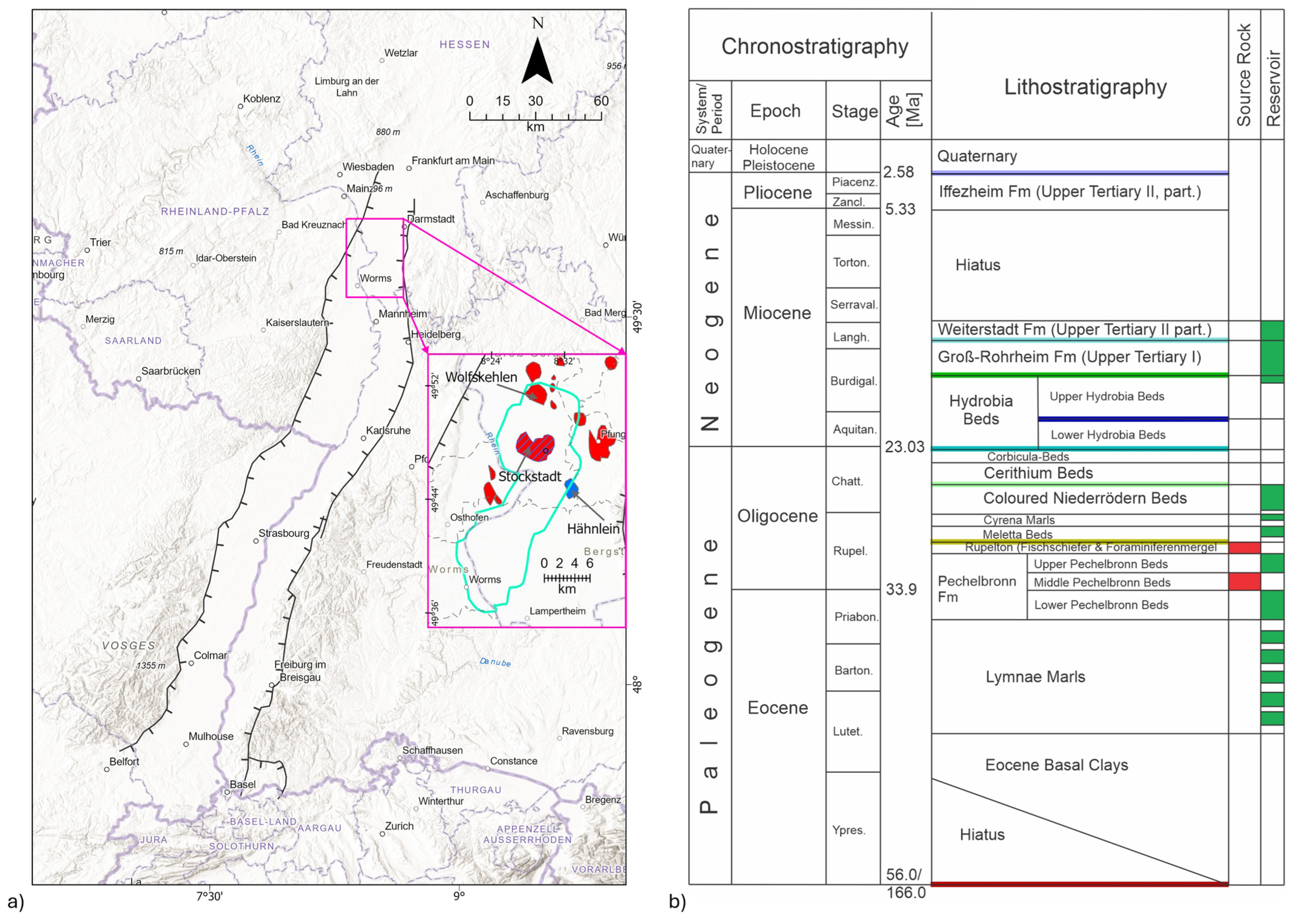
The URG is part of the European Cenozoic Rift System (ECRIS), which stretches for 300 km from Basel to Frankfurt and is linked to the Alpine orogeny (refer to Figure 1a). From the Eocene to the present, the URG has undergone a complex evolution with multiple tectonic phases [26,27].

The stratigraphic column (modified after [28], shown in Figure 1b) shows the lithostratigraphic units that host hydrocarbon reservoirs and the corresponding source rocks. The lithostratigraphic descriptions of the stratigraphic units in the study area are detailed in previous publications [28,29,30]. The gas accumulations in this study area, mainly found in the Hydrobia Beds, Groß-Rohrheim, and Weiterstadt/Iffezheim Fm, serve as gas reservoirs with biogenic natural gas origins. However, the Hydrobia Beds are minor reservoirs, but their bituminous marl clays are crucial as the source of gas. The Miocene sands (Upper Tertiary layers) are also commonly known locally in German as JTI (Jungtertiär I) and JTII (Jungtertiär II).

Hydrocarbon fields produced between the 1950s and 1980s are shown in Figure 1a, along with the cumulative production volumes in

Table 1. Exploration and production history of hydrocarbon fields in the northern URG [28].

Exploration Phases	Gas Field	Year of Discovery	End of Production	No. of Producers	Production [MMm3]	Reservoirs
2nd Phase	Wolfskehlen	1951	1989	21	206.702	Tertiary
	* Subfield Büttelborn	1956				Tertiary
	* Subfield Dornheim	1957				Tertiary
	Pfungstadt	1952	1975	8	161.160	Tertiary
	Stockstadt	1953	1980	26	524.934	Tertiary
	Eich	1955	1973	7	117.834	Tertiary
	Frankenthal	1959	1961	5	20.093	Tertiary
3rd Phase	Darmstadt-SW	1981	1986	1	9.745	Tertiary
Cumulative production [MMm3]					1040.468

* The production of Büttelborn and Dornheim was reported with Wolfskehlen.

. The hydrocarbon exploration history of the German URG commenced with the first hydrocarbon discovery in 1921 [28]. Exploration subsequently progressed through four major phases, resulting in the discovery of numerous oil and gas fields. The gas fields within the study area that were discovered during the second and third exploration phases are listed in Table 1, adapted from [28].

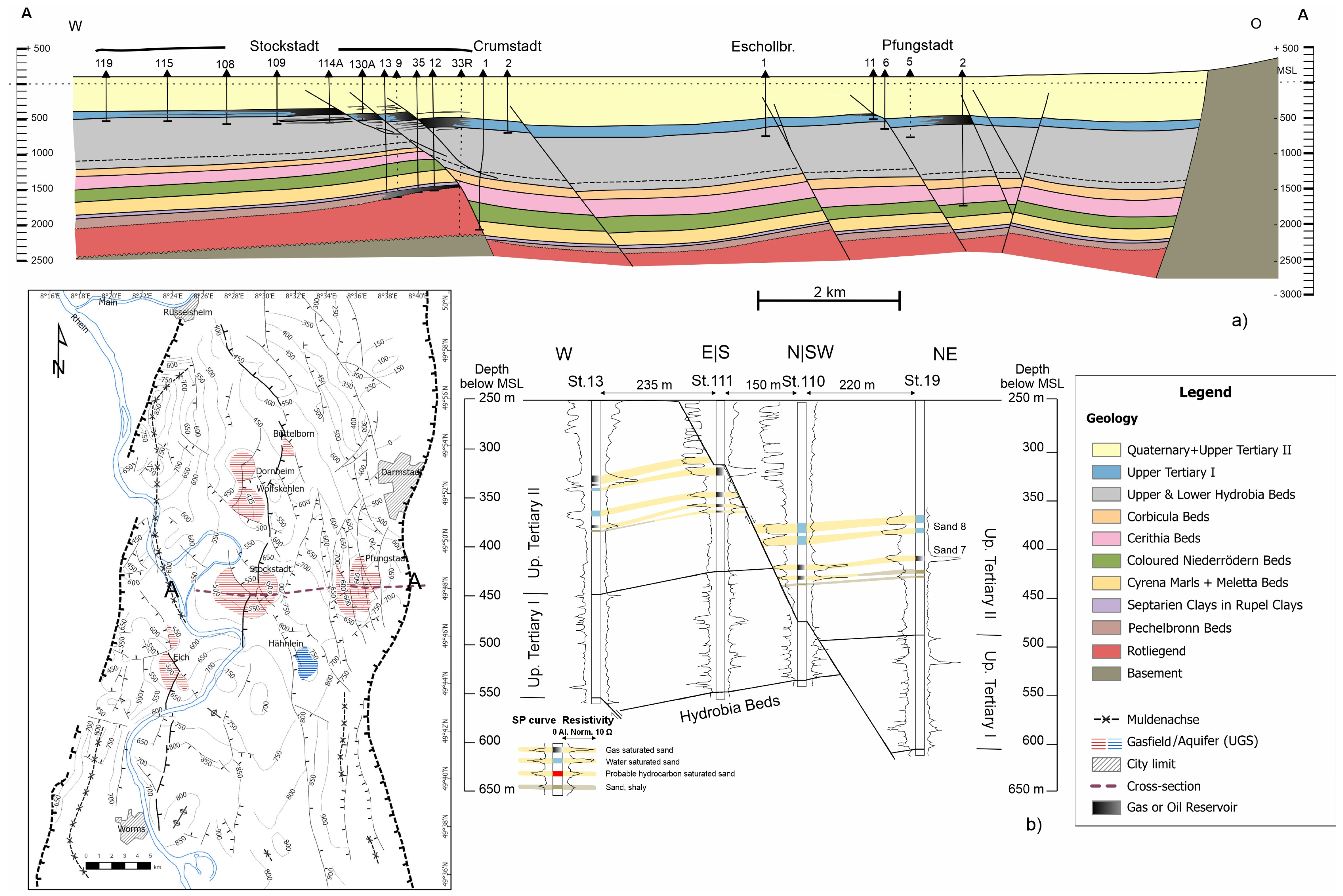
This paper focuses mainly on the reservoir sands of JTI (Groß-Rohrheim Fm) and JTII (Weiterstadt Fm/Iffezheim Fm) of Stockstadt and Hähnlein UGS. Figure 2 illustrates a detailed top-depth structure map of the Upper Hydrobia Beds, drawn during the production period (1962) for this area, along with a semi-schematic cross-section (Figure 2a) that reflects the geological understanding at that time across different production sites and a log correlation panel (Figure 2b) from the Stockstadt area. The cross-section AA illustrates the two stratigraphic units in Stockstadt that produced hydrocarbons. The deeper stratigraphic unit (Pechelbronn Beds) produced oil, and the shallow JTII sands produced biogenic gas. The log panel in Figure 2b, showing the correlation of the various sands, clarifies the thin sand beds and their intercalation with shale layers. According to operational data, well reports, and the published literature [29,30,31], the water-bearing Sand 8 of the Hähnlein structure has been used as a storage facility since 1960, with coal gas (town gas) stored. Later, in 1973, the reservoir was rebuilt to store natural gas. At approximately the same time, the eastern structure of the Stockstadt gas field was also converted to UGS. In Stockstadt, Sand 7 was converted to storage in 1963, followed by Sand 8 in 1970. Stratigraphically, Sand 7 and Sand 8 are part of JTII.

3. Methodology and Database

3.1. Methodology

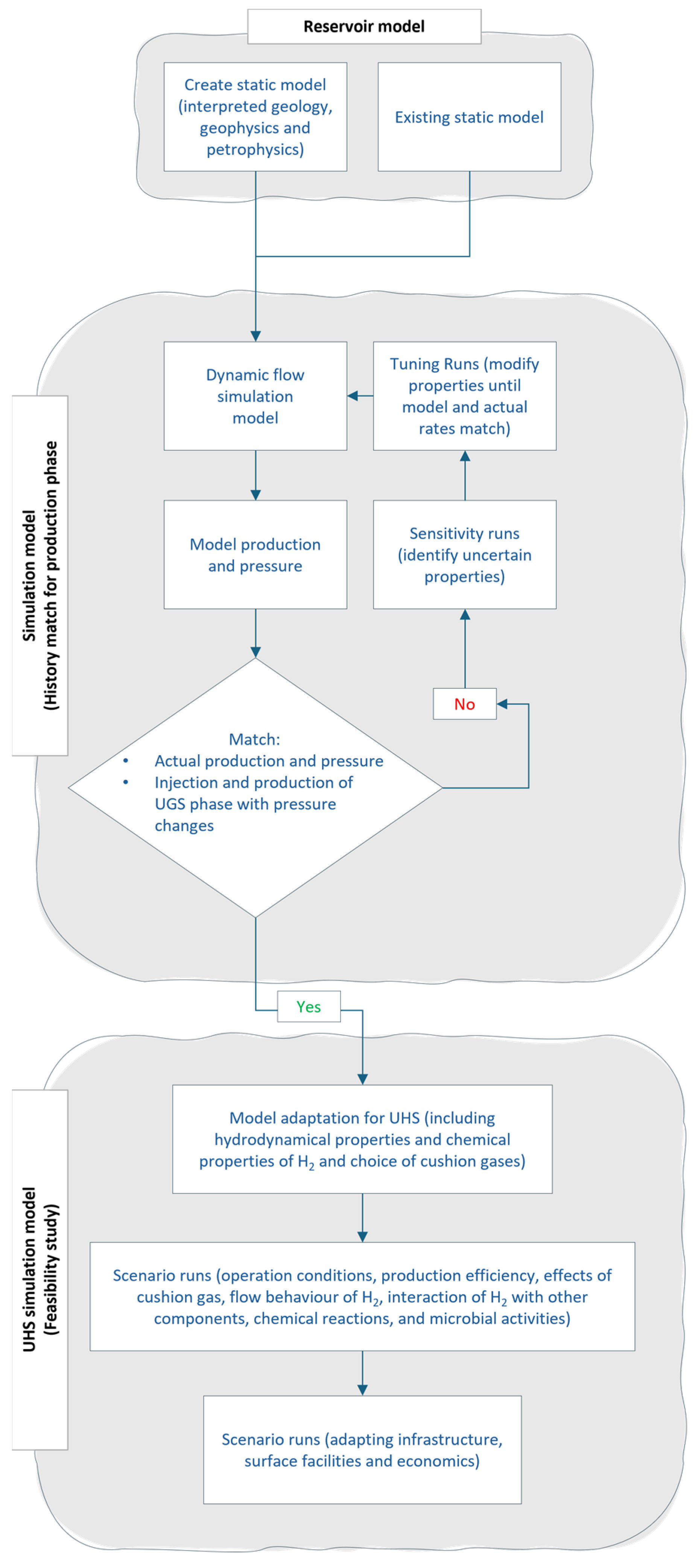
The methodology follows a modified reservoir characterisation and simulation workflow adapted from conventional hydrocarbon field development and UGS studies. The workflow was designed to first establish a calibrated base reservoir model using historical production and UGS data and then adapt it for hypothetical UHS feasibility simulations. The overall workflow is illustrated in Figure 3 and comprises three main stages: reservoir model construction, dynamic model calibration through history matching, and UHS scenario simulation.

The first stage involves developing the reservoir model, which provides the geological and structural basis for subsequent dynamic simulations. Depending on data availability, this model may be generated as either a simplified field-scale tank model or a detailed static geological model based on subsurface data. In this study, a comprehensive dataset was available for the Stockstadt and Hähnlein UGS sites. Well data, including logs and stratigraphic markers, were correlated and calibrated with seismic data to interpret the main faults and horizons. The interpreted structural elements were used to build a regional-scale geological model, from which a field-scale model was extracted. To improve computational efficiency, this field-scale model was converted into a tartan grid, thereby reducing the number of active grid cells while preserving the main structural and reservoir features. While static model building uses the software Petrel™ (v2022.2.0; SLB, Houston, TX, USA) and SKUA-GOCAD™ (v15; AspenTech, Bedford, MA, USA), subsequent dynamic reservoir modelling has been carried out with GEM™ (v2025.10.7.239; Computer Modelling Group, CMG, Calgary, AB, Canada).

The second stage involves constructing and calibrating the dynamic flow simulation model for the historical production and UGS phases. The dynamic model was initialised by assigning reservoir pressure and temperature, gas–water contact, fluid composition, relative permeability functions, and operational schedules for the active wells. Instead of a black-oil simulator, a compositional model was used to explicitly include the properties of hydrogen and other gas components in the dynamic simulation. The model was first set up to reproduce the historical production phase, including gas production and pressure depletion. Subsequently, the UGS phase was simulated by incorporating injection and withdrawal operations and the associated pressure response. As shown in Figure 3, model calibration was carried out through an iterative history-matching process. The simulated production volumes and pressure response were compared against historical field data. The matching criteria included the actual production and pressure behaviour during the production phase, as well as injection and production volumes and pressure changes during the UGS phase. If the simulated results did not satisfactorily match the historical data, sensitivity runs were performed to identify uncertain reservoir parameters that were controlling the mismatch. These parameters were then adjusted during tuning runs until an acceptable match between simulated and observed rates and pressures was achieved. This iterative loop was essential for constraining uncertain properties, including aquifer extent, reservoir connectivity, permeability distribution, and pressure-support behaviour. Once the model reproduced historical production and UGS performance with sufficient accuracy, it was considered a calibrated base case model for further UHS assessment.

The third stage consists of adapting the calibrated dynamic model for hypothetical UHS feasibility simulations. H₂ is added to the gas composition to include the hydrodynamic, thermodynamic, and compositional properties of hydrogen along with other gas components present in the system. In the UHS simulations, the remaining natural gas in the reservoir was treated as CG, or the choice of gas that can be injected as CG, while different WG compositions were tested to evaluate their influence on storage performance. The scenarios were designed to assess operational conditions, recovery efficiency, pressure response, water production, hydrogen flow behaviour, and the interaction between hydrogen and other reservoir components. The scenario simulations provide insight into the feasibility of using the studied reservoir system for hydrogen storage under shallow reservoir conditions. In addition to flow behaviour and production performance, the workflow allows further extensions to include geochemical reactions, microbial activity, and gas–brine–rock interactions where sufficient data are available. Based on the outcomes of the UHS scenario simulations, the model can also be used to support future assessments of infrastructure requirements, surface facilities, and economic feasibility. Thus, the workflow provides a structured approach for moving from a calibrated hydrocarbon/UGS reservoir model toward a field-scale evaluation of UHS feasibility.

3.2. Database

A comprehensive subsurface database was compiled for the selected study area by integrating well, seismic, production, and archival data from institutional and industrial sources. The selected study area is located in the northern URG in southern Hessen and includes several legacy hydrocarbon fields, such as Wolfskehlen, Stockstadt, Pfungstadt, and Darmstadt-SW. The location was chosen for this feasibility study based on comprehensive data, infrastructure, and UGS experience. Over 150 wells have been selected, with drilling reports from the Hessian Agency for Nature Conservation, Environment and Geology (Hessisches Landesamt für Naturschutz, Umwelt und Geologie, short form: HLNUG) providing stratigraphic and lithological data. The selection criterion was the availability of a sufficiently complete stratigraphic succession, with interpreted formation tops extending from the youngest units to the basement, thereby providing a reliable basis for regional horizon correlation. In contrast, the field-scale model relied primarily on wells associated with the area, as these contained detailed reservoir sand markers and wireline log datasets. Additionally, MND Energy Storage Germany GmbH provided 34 2D seismic lines. 3D seismic data covering approximately 10 km × 30 km from Wolfskehlen to Worms, along with a velocity model, was provided by HLNUG. Production histories from the State Authority for Mining, Energy and Geology (Landesamt für Bergbau, Energie und Geologie, short form as LBEG) were added to the database, which provide insights into monthly production but lack specific details on reservoir pressure, production rates, or water cut during the production phase (1950s–1970s) [33]. Some archived reports about the area have been used to characterise the reservoir and reconstruct the production phase [29,30,31].

Lithological descriptions with well markers for the Stockstadt area have been loaded from the drilling reports and correlated with the well markers from Wolfskehlen and Hähnlein. The industry partner provided the top markers of the reservoir sands in the Stockstadt and Hähnlein areas, which were used to delineate the sands in the UGS areas. The lithological description of the reservoir section was transformed into a facies log for sand correlation and facies modelling. Basic log sets of gamma ray, resistivity, and spontaneous potential were used to identify the lithological character of the reservoir. Most of the wells were drilled during the 1950–1980 period and lack a modern log suite.

Table 2. Summary of stratigraphic markers and corresponding seismic markers.

Full Name/Unit	Stratigraphic Markers (Drilling Reports)	Markers (Seismic Interpretation)
Quaternary	kz	QTR
QTR + JTII
Upper Tertiary I	tmiuJI	JTI Top
JTI
Upper Hydrobia Beds	tmiuHyo	OHY Top
OHY
Lower Hydrobia Beds	tmiuHyu	UHY Top
UHY
Corbicula/Inflata Beds	tmiuCo/In	CBS Top
CBS
Coloured Niederrödern Beds	tolu/oloN	BNS Top
BNS
Rupelton	toluB	RT Top
Pechelbronn Fm
Rotliegend	r	Tertiary Base
Rotliegend
Palaeozoic Basement	pzOKBE	Basement Top

summarises the stratigraphic names used in the HLNUG drilling reports, which provide detailed lithologic descriptions and the corresponding seismic horizons interpreted for the study area.

Markers were correlated with seismic reflectors to identify changes in lithology as indicated by the seismic data. The stratigraphic units in the study area primarily comprise clastic sediments, which can be confirmed from well reports and geological descriptions from the published literature. Nine seismic horizons were identified; refer to Table 2: JTII Top, JTI Top, OHY Top, UHY Top, CBS Top, BNS Top, RT Top, Tertiary Base, and Basement Top. The German nomenclature for the horizons was used for simplification because these names are widely used in the scientific community. JTII Top, JTI Top, and OHY Top were locally refined in Stockstadt and Hähnlein based on MND Energy Storage Germany GmbH’s 2D data interpretation. The fault interpretation in the 3D survey was conducted and compared with the 2D interpretation. Time horizons were converted to depth for static modelling, ensuring reliable depth accuracy for shallow horizons, which were tied to the well markers. In contrast, deeper horizons have reduced accuracy due to lateral velocity variations and limited calibration points, though the error remains acceptable.

3.3. Structural Model

A regional model was created using the nine interpreted seismic horizons in the depth domain, covering the areas of Wolfskehlen, Stockstadt, and Hähnlein. The structural framework considers faults that originate from the basement and affect the Quaternary sediments, including those that impact the reservoir zone. This regional model allows for the extraction of field-scale models for dynamic simulation.

A field-scale simulation grid that includes Stockstadt and Hähnlein was extracted from the regional model for history matching of the production and UGS phases, as well as for the feasibility study of potential future UHS conversion scenarios. The cell size in the reservoir zone was 100 m × 100 m × 2 m, totalling 328,860 cells. Local refinement was applied to the UGS areas to capture changes in the dynamic results at fine resolution. In the X and Y directions, the cells were divided by 2, and in the Z direction, they were divided by 4, resulting in a resolution of 50 m × 50 m × 0.5 m, with ~ 1.5 × 10⁶ cells in total.

A simplified approach for the facies model (net thickness) was considered, and two facies types were defined: reservoir facies (Sand) and non-reservoir facies (Shale). Although Sand 7 and Sand 8 were deposited in channel systems, the reservoir characteristics vary laterally and vertically; also, the connectivity between the two sands is difficult to quantify. The gross thickness of the reservoir facies ranges from 5 to 20 m, with a net-to-gross ratio of 0.55 [31]. The reservoir seal forms a 50–55 m thick complex of shales and calcareous claystones at Hähnlein [31]. Lithological descriptions from wells in the JTII reservoir were converted into facies logs and upscaled to the 3D grid using the ‘largest proportion’ approach. Facies continuity was assessed using vertical proportion curves (VPCs). The VPCs calculated layer-wise facies proportions across the grid using upscaled logs at well locations. Vertical variograms for sand were generated from well data; however, for the lateral variogram, assumptions were made considering the continuity and heterogeneity of the sand bodies based on the depositional environment. A spherical variogram model was applied to the sand facies, with a sill of 0.24, horizontal ranges of R₁ = R₂ = 500 m, and a vertical range of R_v = 5 m, without a nugget effect. The facies proportion from the upscaled logs was used as hard data, and the VPCs were used as secondary data to distribute the facies in 3D space using the sequential indicator simulation (SIS) algorithm. A staged modelling approach was adopted to limit the number of poorly constrained parameters during dynamic calibration. Geological heterogeneity was represented through the structural framework and stochastic sand–shale facies distribution. Representative effective reservoir properties were initially assigned to the sand facies, with porosities of 25% for Sand 7 and 30% for Sand 8 and permeability of 1000 mD (k_h)/100 mD (k_v) for both sands, adapted from the published literature [29,30,31]. This simplified parameterisation allowed the full-field model to be dynamically calibrated over the complete production, UGS, and subsequent UHS simulation periods without introducing additional unconstrained petrophysical variability.

3.4. Dynamic Model for History Match of Production and UGS Phase

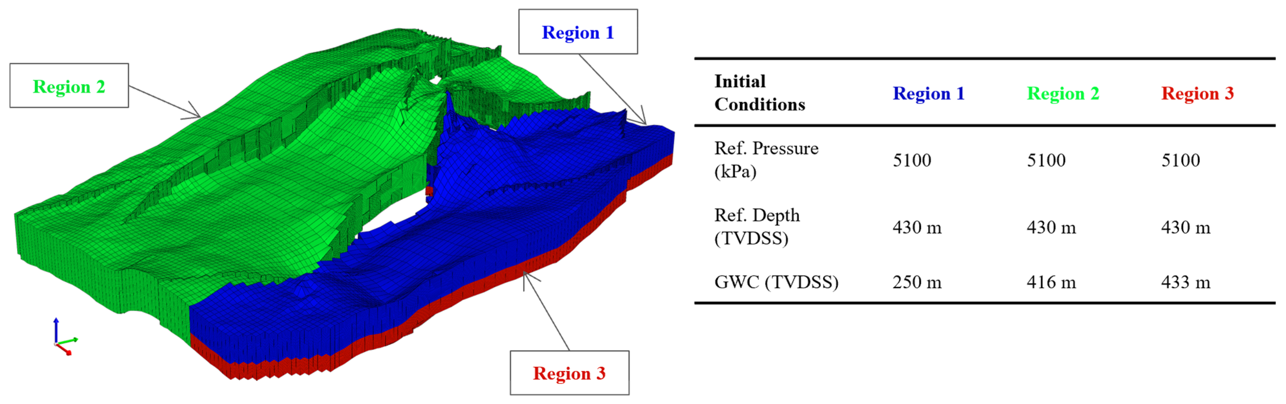
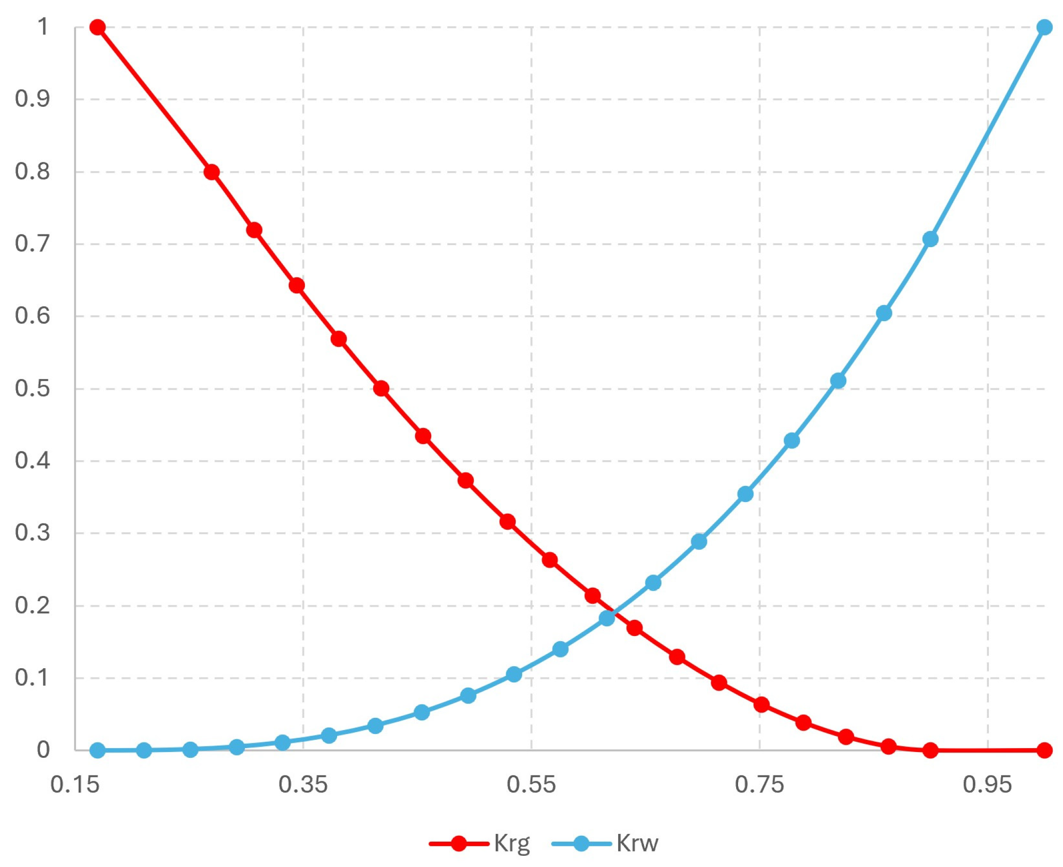
The dynamic model includes the Stockstadt gas field and UGS Hähnlein, initialised on 1 January 1955, utilising LBEG annual reports for the production phase. Sand 7.2 was identified as gas-filled in the UGS Stockstadt, while Sands 8.1 and 8.2 were water-filled. However, all the respective sands in the other fault blocks in the Stockstadt area were gas-filled. Sand 8 in the Hähnlein area was water-bearing on the initialisation date. To effectively manage the configuration of sands, the reservoir grid is divided into three regions to assign the initial conditions for reservoir pressure and gas–water contact (Figure 4). The reservoir sands are locally subdivided into individual subunits (e.g., Sand 7.1 and Sand 7.2, Sand 8.1 and Sand 8.2). Unless differentiation between these subunits is required, they are hereafter collectively referred to as Sand 7 and Sand 8, respectively. The initial reservoir temperature was 29 °C, with an initial pressure of 5100 kPa (51 bar) at a depth of 430 m below MSL. The gas accumulation in the Stockstadt area was of biogenic origin, and it is believed to be a localised, small gas accumulation. Hence, the assumption was made that the initial gas saturation was quite low. Default relative permeability curves for sand from Petrel were used and modified for unconsolidated sands in the absence of reservoir-specific SCAL (special core analysis) measurements. Figure 5 shows the gas–water relative permeability functions used in the dynamic simulations. The adapted curves have a connate water saturation value (S_wc) of 0.17 and a critical gas saturation value (S_gc) of 0.10, with endpoint relative permeabilities of k_rg (gas) = 1.0 and k_rw (water) = 1.0. The Peng–Robinson Equation of State (EOS-PR78) was used in the compositional model. Hysteresis, solubility, diffusion, and abiotic and biotic chemical equations were not incorporated.

A five-component model was used, reflecting gas compositions (94.6% CH₄, 3.0% C₂₊, 2.2% N₂, and 0.2% CO₂) reported in [34] during production, with H₂ included for hypothetical UHS scenarios. A volume multiplier (VM) was applied to the cells below the gas–water contact (433 m) to define the aquifer’s dimensions. The aquifer thickness, lateral extent, and petrophysical properties remain poorly constrained due to the limited availability and age of the existing well-log suites, as well as difficulties in correlating sand bodies below seismic resolution. Data from LBEG spanning 1955 to 1978 indicated 26 producing wells in the Stockstadt area, with gas production rates estimated from their yearly outputs. The individual rates for the wells are not available due to data archival limitations. The LBEG report does not specify the water production rate; however, some of the older literature cites an average water production rate of approximately 100 m³/day at the end of the production phase [30]. The maximum gas production rate per well was assumed to be 6000 m³/day, with a minimum bottom-hole pressure (BHP) of 500 kPa.

The dynamic model was designed to reproduce the production phase as far as permitted by the available archived data and to achieve a more detailed calibration against the subsequent UGS operational period. The production phase is only weakly constrained due to incomplete or unavailable reservoir pressure data and well-specific production histories. In contrast, the UGS period provides substantially better constraints through available pressure, injection, withdrawal, and water-production data (proprietary of industry partner). The calibrated UGS model was therefore used as the principal basis for evaluating the subsequent UHS scenarios. Four aquifer VMs (1000, 10,000, 100,000 and 1,000,000,000) were evaluated, and three are reported in this paper (1000, 10,000 and 100,000).

Although the production phase could be reproduced reasonably well for all cases (aquifer dimensions), the UGS operational period provided a better constraint on aquifer support (100,000 VM). Lower aquifer multipliers underestimated the observed injection and withdrawal performance, whereas increasing the multiplier beyond 100,000 produced only minor differences during history matching. Furthermore, the largest aquifer case did not consistently improve UGS/UHS performance and, in some simulation scenarios, resulted in lower recoverable gas volumes than the 100,000 VM case. Consequently, the aquifer multiplier of 100,000 was adopted as the representative base case for subsequent UGS/UHS simulations.

The UGS conversion of the eastern block of Stockstadt and Hähnlein started in the 1960s. Sand 7.2 was transformed into a gas storage in 1963. Gas injection into Sand 8.1 on the Stockstadt structure began in 1970, shortly followed by the start of injection into Sand 8.2. The Hähnlein facility was first utilised for storage in 1960 when coal gas was injected into the structure. In 1973, the reservoir was modified to store natural gas [31]. The model simulates UGS operations from March 2016 to April 2025. At the Stockstadt UGS, 12 storage wells are operational, while in the Hähnlein UGS, 15 are operational. The injection and withdrawal rates for this time period were downloaded from the company’s official website. These rates were assumed to simulate the approximate conditions of the UGS to the present day. Due to the scope of our work and data confidentiality, actual pressure data, injection, and withdrawal rates for the UGS phase were not simulated; however, an attempt was made to replicate conditions as similar as possible to understand the lifetime of a depleted gas reservoir or saline aquifer.

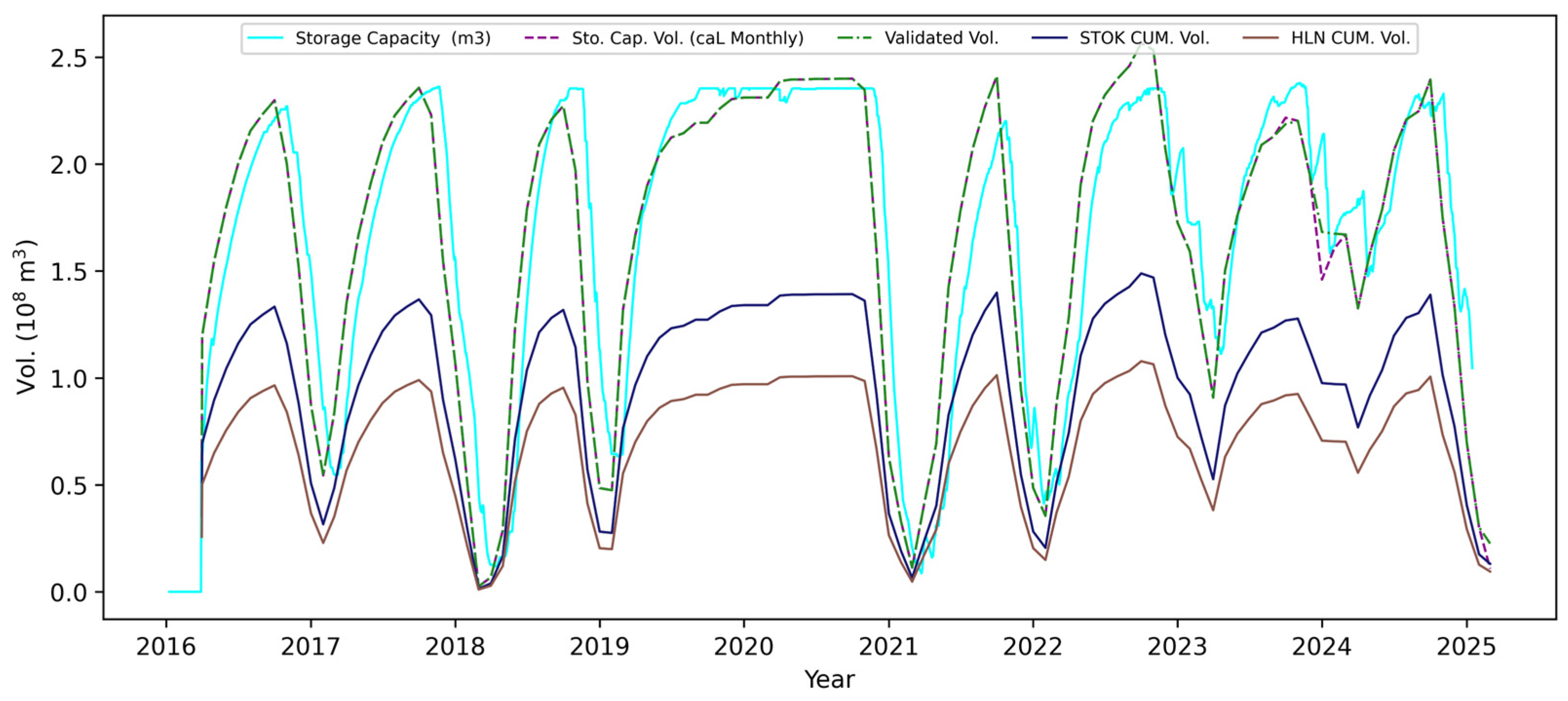
Along with the remaining gas, 50 million cubic meters (MMm³) was injected into Sand 7 as CG for UGS operations. Approximately 38 MMm³ and 80 MMm³ of natural gas with the same composition [34] were injected as CG during the initial setup of Sand 8 at the Stockstadt and Hähnlein UGS sites over 1 year, from March 2014 to February 2015. Following this, a similar volume of WG (Figure 6) was considered in the schedule, along with similar operational conditions (refer to

Table 3. Operational specifications of UGS Stockstadt and UGS Hähnlein.

Parameter	UGS Stockstadt	UGS Hähnlein
Total gas volume (106 m3)	263	153
Working gas (WG) volume (106 m3)	135	80
Cushion gas (CG) volume (106 m3)	128	73
Maximum reservoir pressure (kPa)	6200 (Sand 7)/5500 (Sand 8)	5400 (Sand 8)
Minimum reservoir pressure (kPa)	2500 (Sand 7)/2500 (Sand 8)	2500 (Sand 8)

), which included the number of wells, BHPs, and withdrawal and injection rates, to simulate the interval from March 2016 to March 2025.

In Figure 6, the storage capacity is represented by three curves. The cyan curve shows the actual data, whereas the green curve represents monthly averages calculated by classifying each period according to the dominant operational mode (injection or withdrawal). The magenta curve represents a refined monthly average that additionally accounts for significant withdrawal during an injection-dominated period or significant injection during a withdrawal-dominated period. The magenta curve was selected for constructing the simulation schedule because it better preserves significant injection and withdrawal events that would otherwise be masked by averaging based solely on the dominant monthly operational mode.

Based on the net rock volume (NRV) of Stockstadt UGS, it is assumed that approximately 60% of the WG is from Stockstadt. This volume assumption was considered in the schedule file. The average injection rates for Sand 7 and Sand 8 in Stockstadt UGS are 183,000 m³/day and 61,200 m³/day per well, respectively. The average withdrawal rates for the respective sands are 193,000 m³/day and 65,000 m³/day. For Hähnlein UGS, the average injection/withdrawal rates are 59,000/89,500 m³/day, respectively.

3.5. Dynamic Model for Hypothetical UHS Phase

After this UGS simulation stage, the model was considered as the base case model to test different UHS scenarios. UGS Stockstadt was simulated for 10 years for two cases: (1) 5% H₂ + 95% CH₄ (Case X) and (2) 100% H₂ (Case Y), where the remaining natural gas is considered as CG. Case X was defined as a near-term blending scenario, considering limitations on the hydrogen fraction that can be accommodated within existing natural gas infrastructure and by downstream applications, including the automotive sector. This case therefore represents a storage operation in which hydrogen is introduced while the system remains predominantly based on natural gas. In contrast, Case Y was selected to represent a long-term scenario in which the storage facility is converted from conventional natural gas storage to dedicated hydrogen storage. The two scenarios were conducted over a 10-year period, from April 2025 to March 2034. The injection duration was derived from typical UGS use, with a main period from around April to late October or early November. Production occurs from November through the end of March. A total of 12 storage wells were used for operations (four for Sand 7 and eight for Sand 8). A group target for an injection volume of 650,000 m³/day was set for seven months, resulting in a total injection of 139 MMm³. During the annual cycle, a withdrawal volume of 925,000 m³/day was planned for five months, also totalling 139 MMm³. For Sand 7, the average injection rate is 90,000 m³/day per well, while the average withdrawal rate is 125,000 m³/day per well. In contrast, Sand 8 has an average injection rate of 37,500 m³/day per well and an average withdrawal rate of 73,000 m³/day per well.

4. Results

4.1. Seismic Interpretation and Structural Model

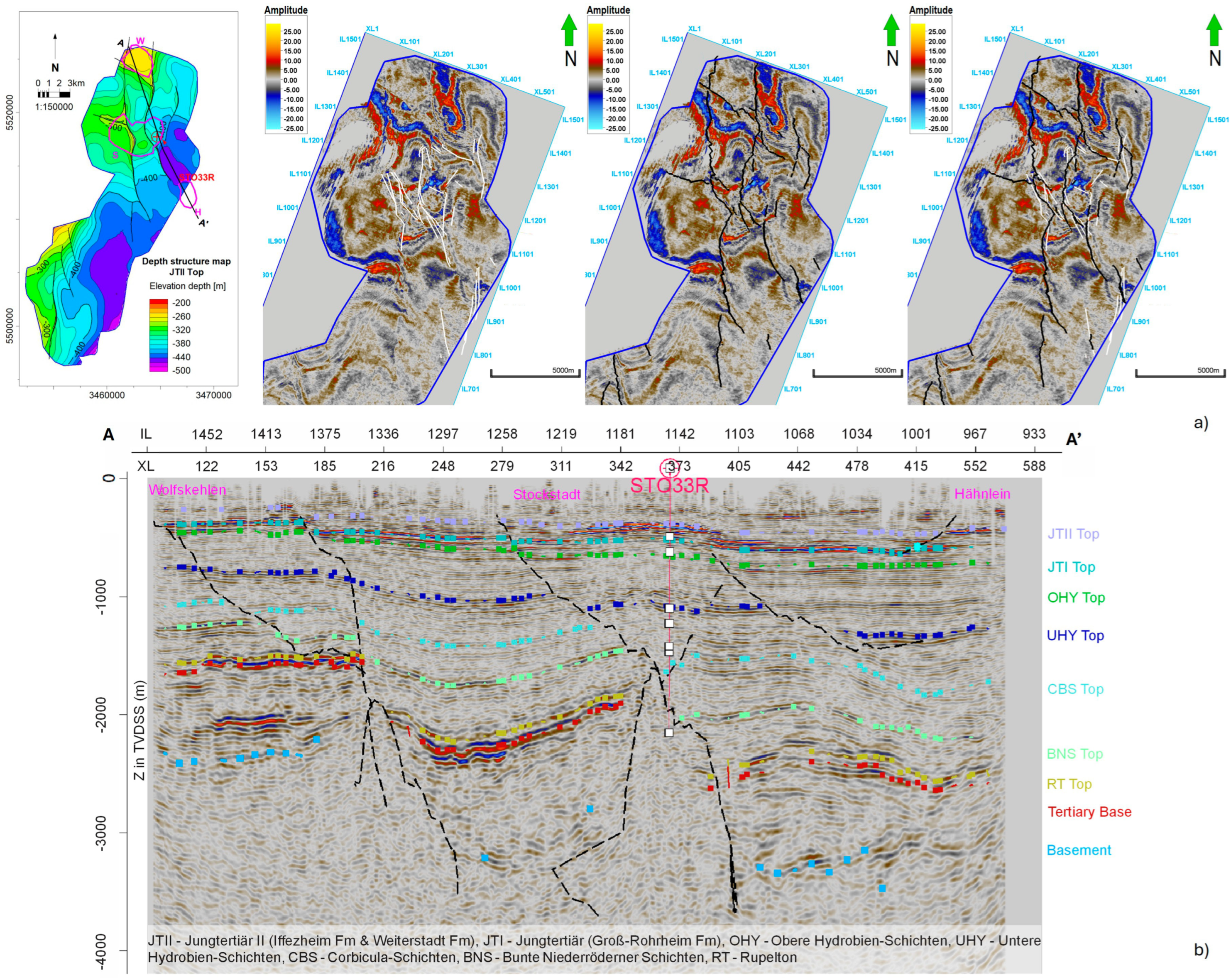
The detailed reinterpretation of the 3D seismic survey allowed for the generation of higher-resolution depth structure maps for the area of interest. This process also enhanced our understanding of the structural configuration of faults within the reservoir zone and in the surrounding regional setup. The shallow horizons (JTII Top, JTI Top, and OHY Top) have minimum time–depth conversion error. The interval velocity, calculated from well markers and time picks at well locations, ranges from 2000 to 2200 m/s, which is applicable for shallow depth zones with clastic sediments. Data from checkshot analysis validate the observation regarding two-way traveltime (TWT). Consequently, the marker calibration of shallow horizons in the velocity model resulted in an improved definition of reservoir structure and a more accurate depth prediction of the sand tops.

Figure 7a depicts the reinterpretation of the data, enabling more accurate identification of the 3D configuration of fault surfaces. Figure 7b displays a seismic section across Wolfskehlen–Stockstadt–Hähnlein, highlighting the interpreted horizons and faults. The basement top picking is incomplete because the seismic reflector is poorly defined laterally. Analyses of sediment thickness maps show a general increase from NW to SE, with local variations driven by fault activity. The interval between OHY Top (18 Ma) and UHY Top (21 Ma) has been analysed and shows significant thickening in the eastern fault block, aligned with periods of increased fault activity. Fault-related depocentres confirm that differential fault movement has caused heterogeneity in sediment thickness and a complex relationship between tectonics and sedimentation (explained in detail in [35]).

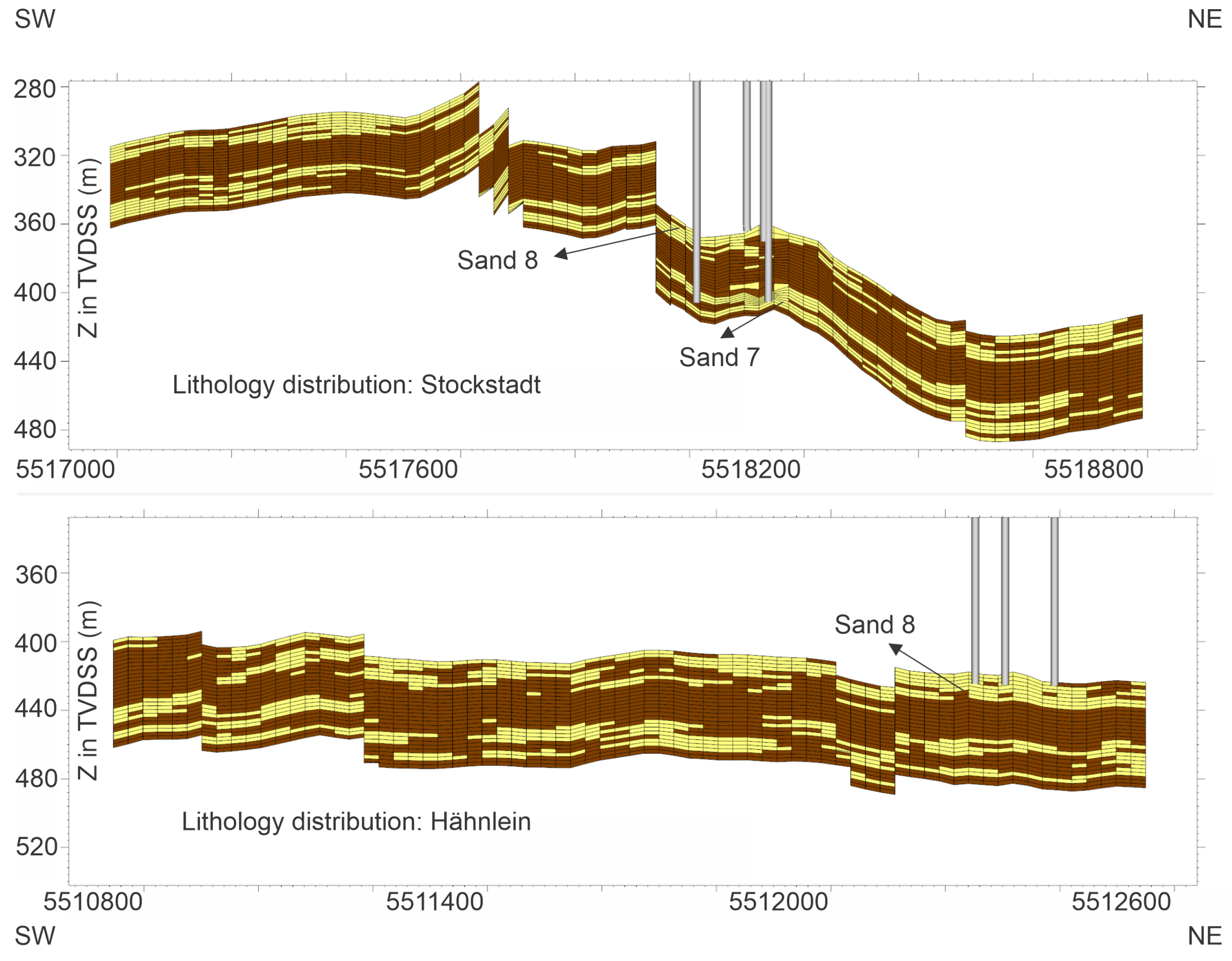
The nine depth-converted seismic surfaces were used to create a general structural model with the most important faults. Furthermore, faults were added to the reservoir grid to improve the compartmentalisation of the zone of interest. The faults are represented as stair-stepped faults to capture more complex structural configurations between two faults and facilitate faster simulation. Figure 8 shows lithological cross-sections through the Stockstadt and Hähnlein reservoirs extracted from the reservoir grid, illustrating the stratigraphic arrangement of the main reservoir units (Sand 7 and Sand 8) and the positions of the storage wells. The facies distribution represents a geologically reasonable realisation of a channelised sandstone system constructed during static modelling and constrained by well data and regional depositional understanding. However, because the channel sands are sub-seismic, their internal geometry and lateral continuity cannot be uniquely resolved from the available seismic data; therefore, the facies architecture shown should not be interpreted as a deterministic description of the subsurface. Multiple stochastic facies realisations were generated during the geological modelling workflow. The realisation selected for dynamic simulation was chosen based on its consistency with well observations and geological continuity. Dynamic calibration was subsequently performed using this representative realisation, which reproduced the observed pressure evolution and injection–withdrawal volumes during the production and UGS operation periods. The influence of alternative facies realisations on dynamic reservoir behaviour was not investigated.

4.2. Dynamic Simulation

The following results should be interpreted in the context of the two-stage calibration strategy adopted in this study. The production phase primarily served to reproduce the overall production behaviour using the limited archived production records available for the field. Due to the lack of continuous reservoir pressure measurements and detailed well-specific production information, the production phase alone does not uniquely constrain the reservoir model. In contrast, the subsequent UGS operational period provides substantially better calibration constraints through the available operational data, including pressure, gas injection, gas withdrawal, and water production. Consequently, the representative aquifer model presented below was selected primarily based on its ability to reproduce the observed UGS behaviour while remaining consistent with the historical production history.

Table 4. Summary of calculations for the net reservoir volume (NRV) and the gas initially in place (GIIP) from the structural and dynamic model.

Reservoir	NRV (106 m3)	Structural Model GIIP (106 m3)	Dynamic Model GIIP (106 m3)	Difference (%)
Stockstadt Gas field	194.0	970	1070	10
Stockstadt UGS (Sand 7)	23.5	118	132	12
Stockstadt UGS (Sand 8)	28.0	–	–	–
Hähnlein UGS (Sand 8)	32.2	–	–	–

compares the NRV and corresponding gas initially in place (GIIP) derived from the structural model with the volumes obtained after dynamic model initialisation for the Stockstadt gas field, the Stockstadt UGS, and the Hähnlein UGS. The Stockstadt gas field volume includes the gas-filled Sand 7 interval within the UGS area, while GIIP for Sand 8 in both UGS sites was not considered during initialisation because these intervals were water-bearing. Differences of approximately 10–12% are observed between the two model representations. Given the limited well control, the difficulty of resolving sub-seismic reservoir heterogeneity, and the simplifications introduced during dynamic model construction, these limitations are interpreted as reflecting uncertainties associated with model discretisation, facies representation, property assignment, and initialisation rather than as a measure of the absolute uncertainty in reservoir GIIP. The comparison is therefore used primarily as a consistency check between the static and dynamic model representations.

This consistency is further supported by the production match: the dynamic simulation yields 63 MMm³ of cumulative production from the Stockstadt UGS compared with 57 MMm³ of actual production (+10%) [31], and 500 MMm³ simulated versus 525 MMm³ actual cumulative production for the Stockstadt gas field.

During the production phase, field operation was controlled by constraints on maximum daily gas production, minimum BHP, and maximum allowable water production rate. Under these operational controls, the dynamic model closely reproduces the reported number of producing wells and the overall production duration of the field, consistent with the published LBEG report. This further supports the reliability of the model in representing both volumetric and operational aspects of the historical field development.

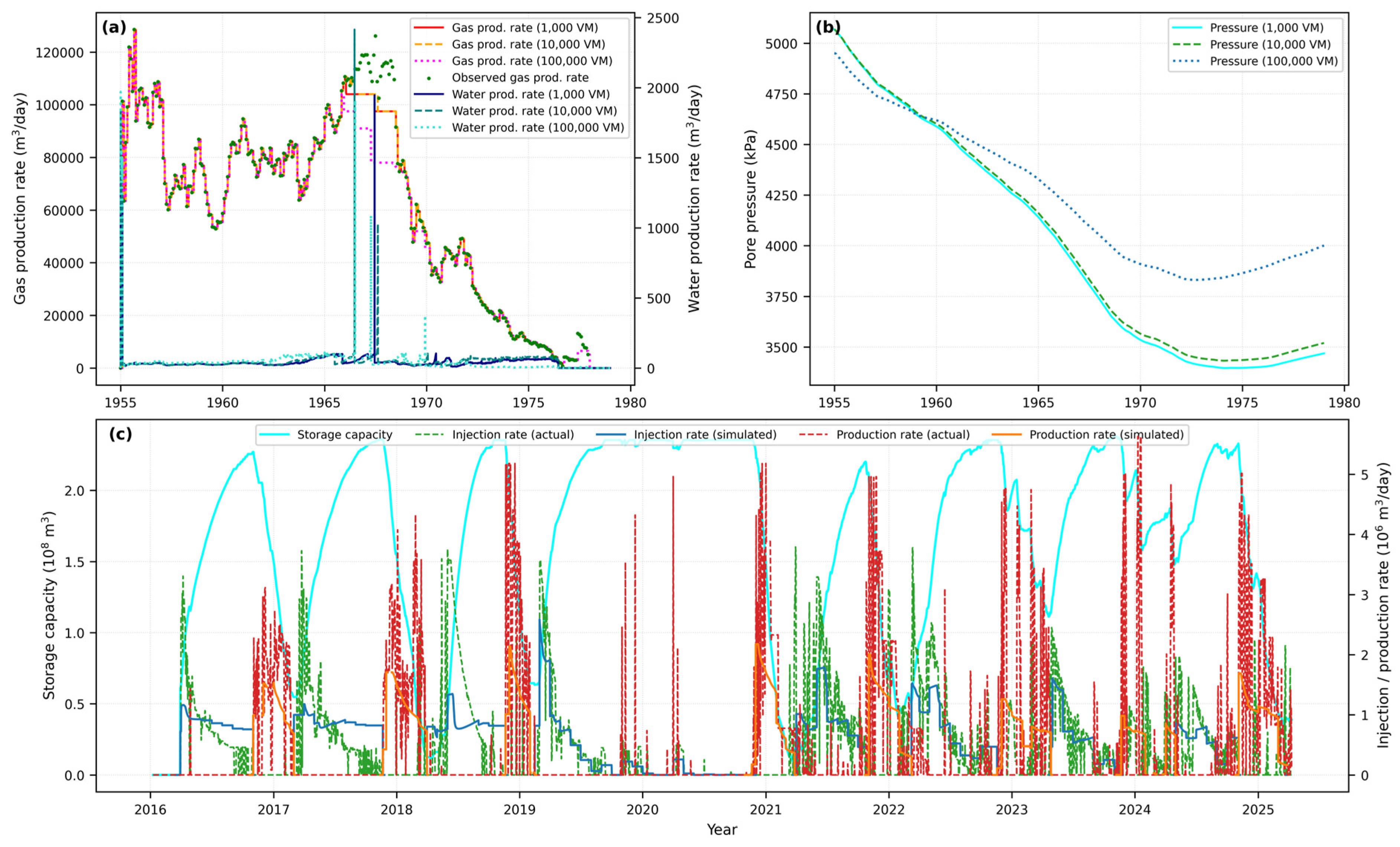
The aquifer strength played an important role in the calibration of volumes, water production, and pressure development. Figure 9a presents the results of the aquifer sensitivity analyses conducted for the production phase from 1955 to 1978. Simulated gas and water production rates for three aquifer strength scenarios—weak (1000 VM), medium (10,000 VM), and strong (100,000 VM)—are compared with observed gas production data. Aquifer strength was varied by applying a VM to the aquifer layers below the gas–water contact (GWC), representing different effective aquifer sizes and degrees of hydraulic support. Among the tested cases, the strong aquifer scenario provides the best agreement with the observed production volumes.

Figure 9b shows the simulated reservoir pressure evolution for the three aquifer strength scenarios during the production phase. While all cases exhibit a pressure decline associated with gas production, the magnitude and timing of the decline depend strongly on aquifer strength. In the weak aquifer case (1000 VM), pressure decreases rapidly and reaches limiting levels at an earlier stage, leading to premature termination of production. The medium aquifer scenario (10,000 VM) delays this pressure depletion but still results in an earlier production stop compared with the strong aquifer case. In contrast, the strong aquifer scenario (100,000 VM) maintains higher pressure levels over a longer period, allowing production to continue for an extended duration. This behaviour is consistent with Figure 9a, where production rates are broadly similar across all aquifer scenarios during active production, but the weaker aquifer cases cease production earlier (red and orange curves). Although direct pressure measurements are not available for validation of the production phase, the smoother pressure evolution associated with the strong aquifer case is consistent with its improved ability to sustain production and storage volumes in the dynamic simulations.

The calibrated model (100,000 VM) was subsequently applied to simulate the UGS operational period from 2016 to 2025. Figure 9c compares simulated and observed storage capacity, injection volumes, and withdrawal volumes for the Stockstadt and Hähnlein UGS sites. While the production phase alone did not uniquely constrain aquifer strength because of the limited availability of archived production data for each well, the UGS operational period provided substantially better calibration constraints. The dynamic model was therefore calibrated against the available UGS operational dataset, including pressure, gas injection, gas withdrawal, and water production. Among the investigated aquifer strength cases, the VM = 100,000 model provided the representative base-case aquifer representation, achieving the best agreement with the available historical and UGS operational data within the constraints of the available dataset. This calibrated model was subsequently adopted as the base case for the UHS simulations.

4.3. Hypothetical UHS Simulation

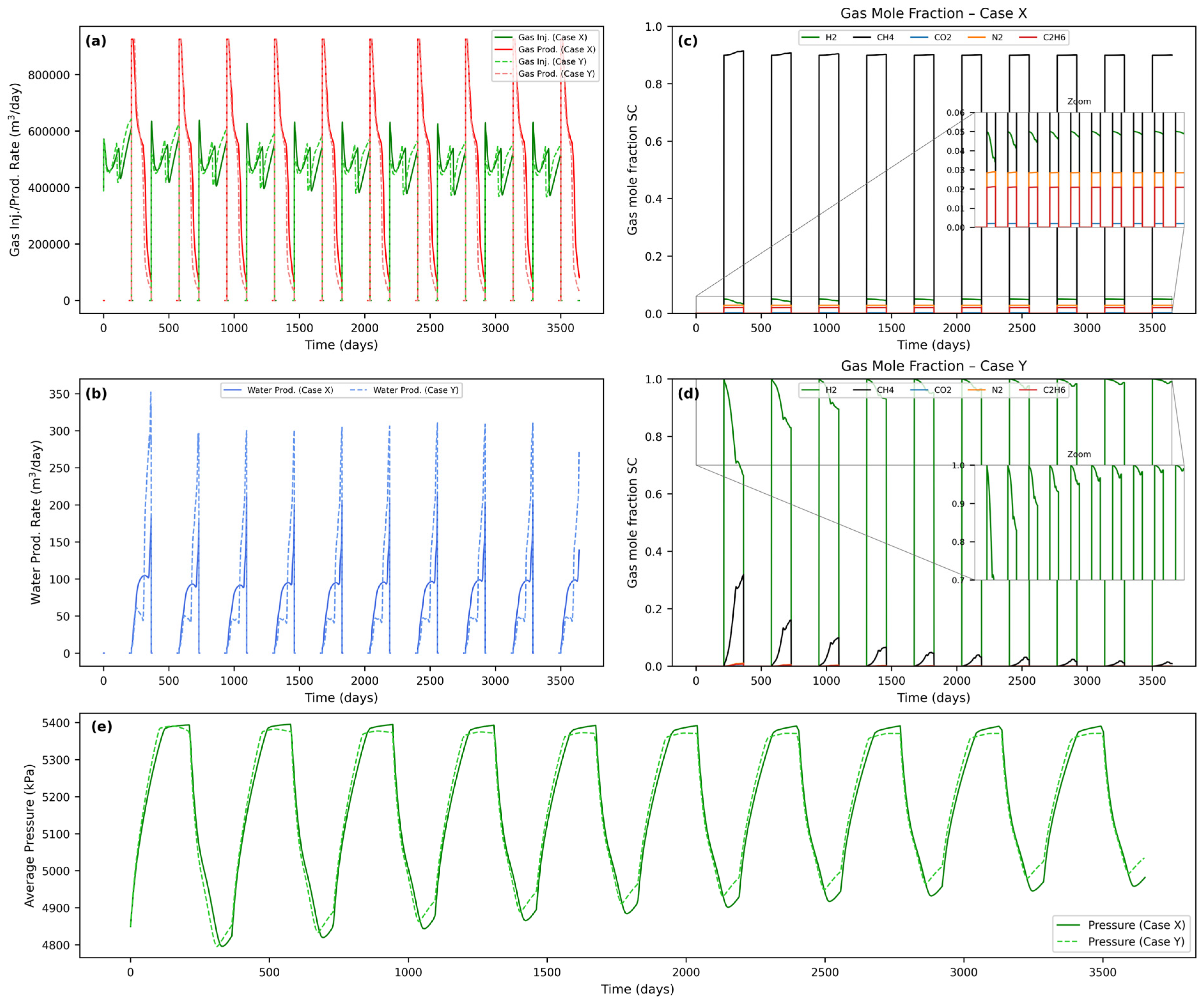
After calibration of the production and UGS phases, the model was initialised for UHS scenarios. Two bounding operational scenarios were investigated. Case X (5% H₂ + 95% CH₄) represents a near-term transitional storage concept involving limited hydrogen blending, whereas Case Y (100% H₂) represents the long-term end-member corresponding to complete conversion of the storage site to hydrogen. The objective was not to evaluate the full range of intermediate blending ratios but rather to establish the expected operational envelope between a realistic transition scenario and a fully converted hydrogen storage system. Figure 10 compares the simulation results for the two UHS cases at the Stockstadt UGS over a ten-year cyclic operation. In both cases, injection and production volumes are of comparable magnitudes, with injection volumes of approximately 100 MMm³ and production volumes of approximately 66–79 MMm³ per cycle. However, Case Y exhibits slightly lower gas production volumes with sharp peaks (Figure 10a) and higher water production rates (Figure 10b) compared with Case X. This behaviour can be attributed to the different thermophysical properties of the WG and the resulting differences in reservoir flow behaviour. In Case Y, the higher hydrogen content results in lower gas density, high mobility, less stable gas–water displacement behaviour, and reduced volumetric storage efficiency under reservoir conditions. Consequently, greater water encroachment occurs during withdrawal, leading to increased water production and slightly lower recoverable gas volumes. In contrast, Case X benefits from stronger effective pressure support, resulting in lower water production and slightly higher gas recovery per cycle, as the WG composition is similar to the CG (natural gas).

The compositional response of the produced gas is shown in Figure 10c,d. In both cases, the H₂ mole fraction in the production stream increases rapidly and remains high from the third cycle onward (Figure 10c,d), indicating efficient displacement of the initial gas inventory, cyclic behaviour, and a quasi-steady state. Despite the observed differences in volumetric performance and water production, both scenarios demonstrate the technical feasibility of sustained H₂ withdrawal with high H₂ purity after the initial conditioning cycles. The pressure response (Figure 10e) shows that both scenarios remain within a similar cyclic pressure envelope because both retain the remaining natural gas as CG from the preceding UGS operation. Nevertheless, slight differences in pressure evolution are observed, reflecting the different pressure–volume behaviour and flow characteristics of the H₂-rich WG compared with the natural gas–H₂ mixture.

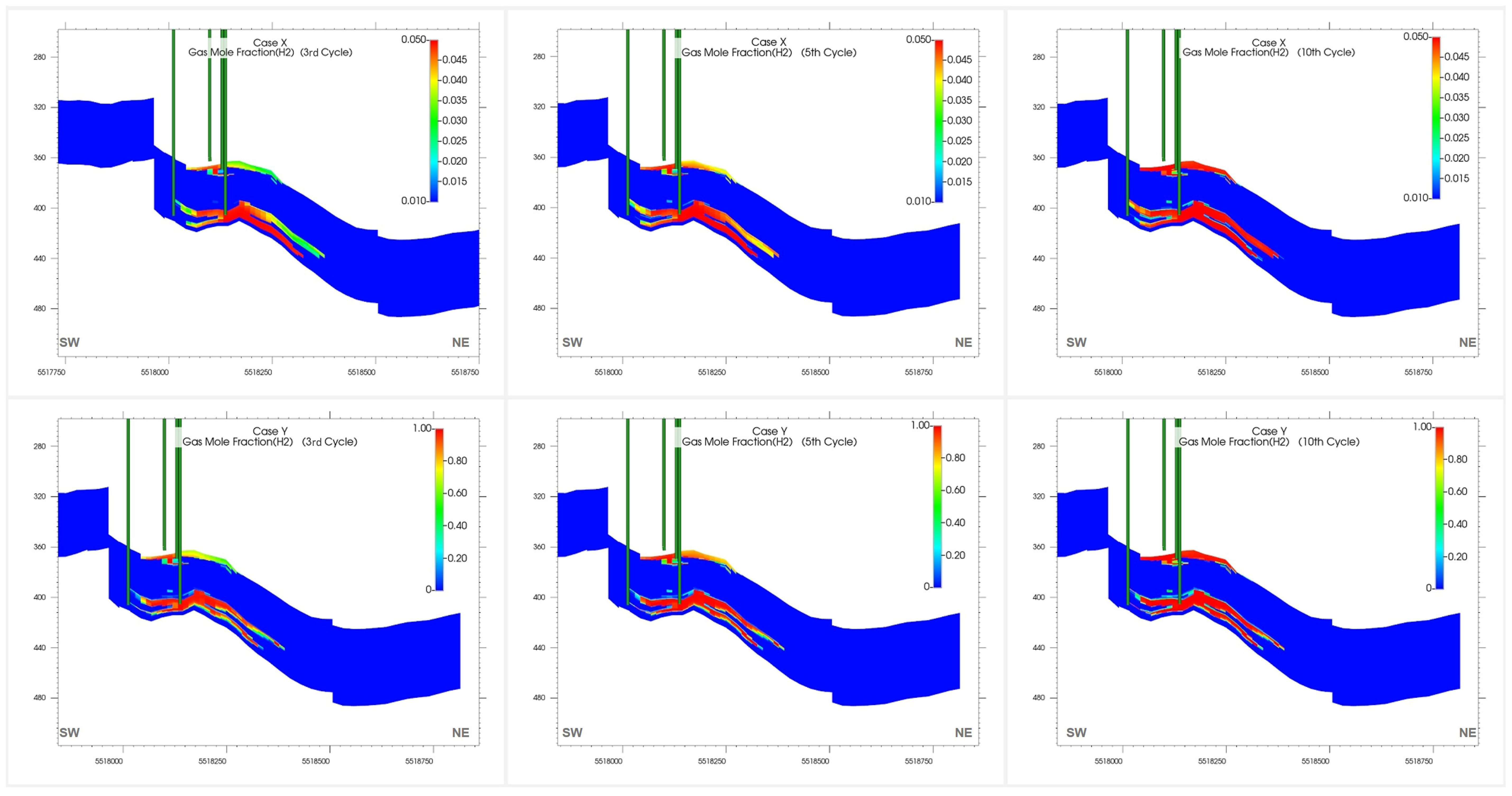
The cycle-wise results in

Table 5. Cycle-wise comparison of Case X and Y summarising cumulative injected volume, cumulative withdrawal volume, average produced H₂ mole fraction, and cumulative water production.

	Case X				Case Y
Cycle no.	Cum. Inj (H2 + CH4) (106 m3)	Cum. with (H2 + CH4) (106 m3)	Avg. Prod. H2 Mol. Frac.	Cum Wat. Prod. (103 m3)	Cum. Inj (H2) (106 m3)	Cum. with (H2) (106 m3)	Avg. Prod. H2 Mol. Frac.	Cum. Wat. Prod. (103 m3)
1	106	78	0.042	14	112	71	0.81	18
2	110	79	0.046	12	110	69	0.91	15
3	106	78	0.047	12	109	67	0.945	14
4	105	78	0.048	12	107	67	0.963	14
5	104	78	0.049	12	106	67	0.973	14
6	103	77	0.049	13	104	67	0.979	14
7	103	78	0.049	12	104	66	0.984	15
8	102	77	0.0495	13	103	66	0.988	14
9	102	78	0.0495	13	103	66	0.991	15
10	102	76	0.0496	11	103	66	0.993	10

complement the spatial H₂ mole-fraction distributions shown in Figure 11. The tabulated values quantify the evolution of injected and withdrawn H₂ volumes, produced H₂ mole fraction, and water production, whereas the cross-sections illustrate the corresponding redistribution of H₂ within the reservoir. In Case X, the average H₂ mole fraction of the produced gas gradually increases from 0.042 in the first cycle to 0.0496 in the tenth cycle, approaching the injected H₂ fraction of 0.05, while withdrawal volumes remain relatively stable at approximately 76–79 × 10⁶ m³ per cycle. In Case Y, the produced H₂ mole fraction increases more rapidly from 0.81 in the first cycle to 0.945 in the third cycle and to 0.993 in the tenth cycle, indicating progressive displacement of the remaining natural gas CG and increasing H₂ enrichment of the produced gas. However, the withdrawal volume decreases from 71 × 10⁶ m³ in the first cycle to approximately 66 × 10⁶ m³ in the later cycles, remaining below that of Case X. Approximately half of the simulated water production originates from Sand 7. In both scenarios, the intended injection and withdrawal targets are not fully attained because well operation is initially restricted by the imposed water-production constraint and, during later stages of the cycles, by the BHP constraint.

From the third to the tenth cycle, the H₂-rich region progressively expands within both Sand 7 and Sand 8, consistent with the increasing H₂ contribution to the produced gas reported in Table 5. However, the spatial response differs between the two reservoir units because Sand 7 and Sand 8 are hydraulically separated and are subject to different aquifer conditions. Sand 7 is influenced by stronger aquifer support (due to VM), whereas aquifer support in Sand 8 is more limited and less constrained by the VM representation. Consequently, the distribution is primarily interpreted in terms of field-scale H₂ migration and compositional redistribution rather than localised near-well coning. The increased water production observed in the pure-H₂ case is consistent with previous numerical studies demonstrating that water encroachment and upconing can significantly influence H₂ withdrawal from aquifer-supported porous reservoirs. The magnitude of this response depends on gas–water displacement characteristics, aquifer support, operational constraints, and the presence and composition of cushion gas [36]. Although water production is evident from the dynamic results in Table 5, localised gas or water coning cannot be reliably identified from these cross-sections because the lateral resolution of the field-scale grid, despite local refinement, is insufficient to resolve the detailed near-well cone geometry.

4.4. Analogue-Based Volumetric Screening

Based on hypothetical UHS simulation results for the Stockstadt UGS, a probabilistic, map-based volume estimation was conducted for the other known former gas fields in the area, i.e., the Wolfskehlen, Pfungstadt, Eich, and Darmstadt fields. The analogue-based probabilistic assessment was intended as a regional screening exercise to rank former gas fields for future detailed geological and dynamic investigations. Field areas were derived from published structural maps (Figure 2), while thickness, porosity, and gas saturation were assigned representative mean values from the Stockstadt–Hähnlein analogue model. Uncertainty was propagated via Monte Carlo simulation using a uniform distribution for area (±20%), a triangular distribution for thickness (5–15 m, mode 10 m), and normal distributions for porosity (μ = 0.25, σ = 0.05) and gas saturation (μ = 0.70, σ = 0.0875). The selected probability distributions reflect the level of information available for each parameter. Uniform distributions were applied where only uncertainty bounds could be estimated (area); triangular distributions were applied where minimum, maximum, and most likely values were available (thickness); normal distributions were applied where the parameter was expected to vary around a representative mean value (porosity and gas saturation).

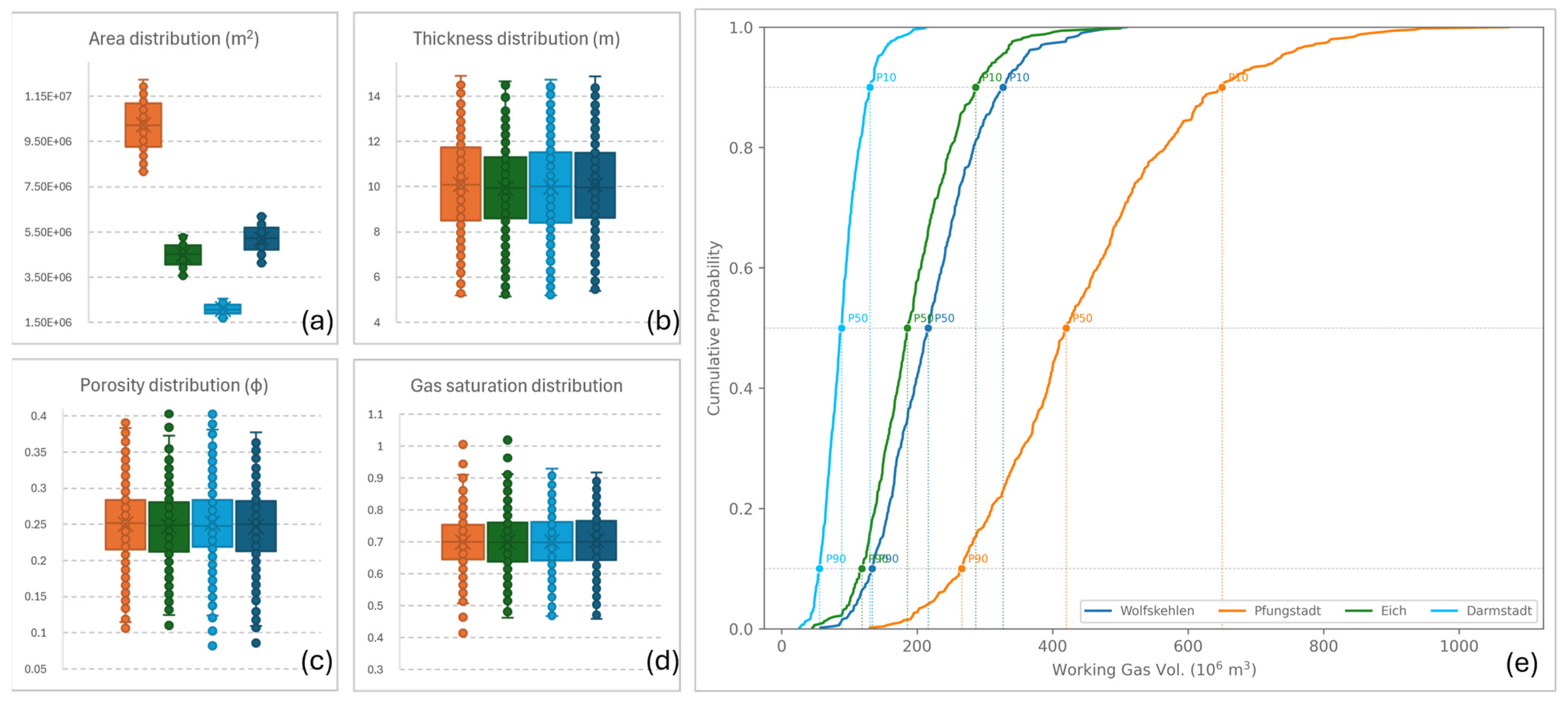
Figure 12 combines input-property variability (box-and-whisker plots) with resulting cumulative distribution functions (CDFs) of the WG volume. The boxplots demonstrate that area (Figure 12a) exhibits the largest inter-field variability, whereas thickness (Figure 12b), porosity (Figure 12c), and gas saturation (Figure 12d) show broadly comparable distributions across all fields. Consistently, the CDFs (Figure 12e) indicate that the differences in GIIP are primarily controlled by areal extent, with Pfungstadt displaying the highest volumes and widest uncertainty range and Darmstadt exhibiting the lowest and most constrained uncertainty range.

The aggregate probabilistic volumes are P90 = 575 × 10⁶ m³, P50 = 910 × 10⁶ m³, and P10 = 1.39 × 10⁹ m³, corresponding to approximately 5.61, 8.89, and 13.62 TWh of CH₄ (1 TWh = 102,359,965.88 m³), respectively (equivalent to 1.87, 2.96, and 4.54 TWh of H₂) [37]. The relatively steep CDF slopes for Eich and Wolfskehlen reflect lower uncertainty, whereas the broader spread for Pfungstadt highlights higher structural uncertainty (highly faulted structure) associated with the area. However, the CDF slope for Darmstadt is the steepest, possibly because the area distribution has a very narrow spread, which contributes to the steep CDF curve. The Wolfskehlen structure represents a promising candidate for further evaluation because it is covered by the available 3D seismic survey, contains some wells with wireline logs, and exhibits geological characteristics comparable to the Stockstadt–Hähnlein analogue. Based on initial log analysis, the correlated sands have similar thickness ranging from 5 to 15 m. Unlike the remaining fields, Wolfskehlen forms part of the regional structural model developed in this study and therefore represents the most suitable candidate for future field-scale dynamic simulations. The volume estimates (P50: 216 × 10⁶ m³ ≈ 2.11 TWh of CH₄ ≈ 0.70 TWh of H₂) fall within the range of the analogue sites. The presented volumes should therefore be interpreted as prospective geological volumes derived from analogue-based probabilistic assessment rather than recoverable working-gas capacities under cyclic hydrogen storage operation.

5. Discussion of Model Uncertainties

The present study establishes a representative analogue model that reproduces the available geological and operational observations. Future developments should progressively reduce uncertainty by incorporating increasingly detailed geological, petrophysical, dynamic, and geomechanical constraints.

Geological uncertainty in the model is primarily related to subsurface interpretation and property representation. Earlier 2D seismic interpretations were refined using the available 3D seismic data, resulting in an improved structural framework and reduced uncertainty in horizon and fault interpretation. However, sub-seismic features such as the internal geometry and lateral continuity of channelised sand bodies cannot be uniquely resolved, and the facies distribution therefore represents a single geologically plausible realisation rather than a deterministic description. Petrophysical property heterogeneity is further simplified by assigning constant porosity and permeability values to the reservoir units, which does not capture small-scale spatial variability but is considered appropriate for the analogue-model objective of this study. Although hydraulic communication between the Stockstadt and Hähnlein reservoirs was reported in the 1980s, this connectivity could not be reproduced in the current model, likely due to limitations in resolving subtle structural or stratigraphic pathways at the available data resolution. These uncertainties are characteristic of legacy reservoirs and are explicitly acknowledged in the static model construction. Nevertheless, the representative base model provides a framework for future investigations incorporating quantitative fault transmissibility and seal-capacity analyses, as well as coupled geomechanical modelling to evaluate fault reactivation, potential leakage pathways, and long-term containment integrity during cyclic hydrogen storage.

Dynamic uncertainty is mainly associated with data availability and scope-related limitations. The dynamic model was validated against publicly available operational data from the UGS period. Within the scope of this study, validation focused on reproducing cumulative production and injection volumes together with the overall field production history. Nevertheless, the available data provide a suitable basis for assessing the model’s field-scale performance. As a result, the model was not calibrated to reproduce short-term operational transients or pressure responses. Despite these limitations, the dynamic simulations provide internally consistent behaviour and reproduce volumetric trends within uncertainty ranges. The model is therefore considered fit for purpose as an analogue framework to assess general storage behaviour in porous reservoirs of the northern URG, while recognising that site-specific operational studies would require additional data and further calibration. Further uncertainty is associated with reservoir-scale processes not explicitly incorporated in the present model, including relative permeability hysteresis, H₂ solubility and diffusion, viscous fingering, and abiotic and biotic geochemical reactions. These processes may affect hydrogen migration, trapping, recovery, and compositional evolution and should be evaluated during subsequent site-specific UHS assessments. In addition, potential H₂-related material degradation and embrittlement of wells and surface infrastructure require separate integrity assessments prior to storage conversion.

Further, the map-based volume estimation approach for the nearby legacy fields implicitly assumes spatial uniformity within each field and does not fully capture intra-reservoir heterogeneity, such as facies variations, compartmentalisation, or localised petrophysical anomalies. The use of independent input distributions does not account for possible correlations between parameters (e.g., porosity–permeability relationships or thickness–facies trends), which may bias the resulting volume distributions. Such heterogeneities may lead to deviations from the modelled distributions, particularly affecting effective porosity, net thickness, and fluid distribution. Consequently, while the probabilistic framework captures first-order uncertainty, the results should be interpreted as screening-level volume estimates, not potential, with the understanding that additional subsurface data (e.g., seismic refinement, well control, and facies modelling) could significantly reduce uncertainty, particularly in defining structural closure and reservoir continuity.

6. Conclusions

This study developed and validated an integrated geological and dynamic model workflow to evaluate UHS potential in shallow, porous reservoirs in the northern URG. To do an initial assessment, an analogue model representing the Miocene sands of the northern URG was developed, incorporating both Stockstadt and Hähnlein UGS. The integrated geological model successfully reconstructed the structural framework and provided a reliable basis for history matching and UHS prediction.

The validated field-scale model provides an analogue for evaluating hydrogen storage behaviour in shallow porous reservoirs while accounting for structural complexity, facies heterogeneity, and aquifer support. The dynamic simulation results of the production and UGS phases emphasise that the dimension of the aquifer plays a significant role for these shallow reservoirs, providing pressure support and also maintaining storage capacities. The hypothetical UHS scenarios of Stockstadt UGS compare two WG options: i) low-H₂ content (5%, natural gas mixture) and ii) pure-H₂ (100%). The prediction for the case with low-H₂ (5%) content shows stable flow with less water production, similar to natural gas; however, the pure-H₂ scenario exhibited greater gas mobility and higher water production than the low-H₂ mixture. This behaviour is primarily attributed to the different thermophysical properties and multiphase-flow behaviour of hydrogen under the investigated reservoir conditions. Compared with the natural gas–H₂ mixture, the pure-H₂ case resulted in increased water production and slightly lower recoverable gas volumes while maintaining a similar cyclic pressure envelope. Despite these differences, both scenarios achieved WG capacities comparable to those of existing natural gas storage operations. These findings demonstrate that depleted hydrocarbon fields and saline aquifers in similar geological settings can be used for seasonal hydrogen storage with only moderate operational modifications, provided that reservoir-specific hydrodynamic behaviour is properly considered.

This work demonstrates the value of integrating legacy hydrocarbon production data, operational UGS data (Stockstadt and Hähnlein UGS facilities), modern seismic interpretation, and dynamic compositional simulation within a single workflow. Such an integrated approach provides a framework for constraining uncertainty in UHS feasibility assessments and offers a transferable methodology for evaluating nearby porous reservoirs, including depleted gas fields and saline aquifers, with comparable geological settings and data limitations. As some of the depleted gas fields, such as Wolfskehlen, have similar geological settings, map-based estimation yields a volume capacity comparable to that of the other two UGS sites. Similar field-scale models for other nearby gas fields or potential prospects can be extracted for hypothetical UHS simulations to test various CGs, geochemical reactions, and methanation. Future work should extend the integrated workflow by coupling the dynamic reservoir model with geomechanical simulations to evaluate well integrity, caprock stability, fault reactivation, surface deformation, and operational pressure limits during hydrogen storage. By enabling the identification of suitable storage sites in the northern URG, this approach supports the development of regional hydrogen infrastructure and contributes to the energy transition and long-term sustainability.

References

1. Al-Shafi, M.; Massarweh, O.; Abushaikha, A.S.; Bicer, Y. A review on underground gas storage systems: Natural gas, hydrogen and carbon sequestration. Energy Rep. 2023, 9, 6251–6266. [Google Scholar] [CrossRef] [Scilit]
2. Katz, D.L.; Lee, R.L. Natural Gas Engineering: Production and Storage. 1993. Available online: https://journals.flvc.org/cee/article/view/123795 (accessed on 13 January 2026).
3. Evans, D.J.; Chadwick, R.A. Underground Gas Storage: Worldwide Experiences and Future Development in the UK and Europe. 2009. Available online: https://www.semanticscholar.org/paper/Underground-gas-storage-%3A-worldwide-experiences-and-Evans-Chadwick/faa31e2fa4929f5c7c638cc243126d4acabfa2a2 (accessed on 13 January 2026).
4. Małachowska, A.; Łukasik, N.; Mioduska, J.; Gębicki, J. Hydrogen Storage in Geological Formations—The Potential of Salt Caverns. Energies 2022, 15, 5038. [Google Scholar] [CrossRef] [Scilit]
5. Underground Sun Storage—Contact—Project. Available online: https://www.underground-sun-storage.at/en/project/contact.html (accessed on 16 July 2023).
6. Hychico. Available online: https://hychico.com.ar/en/underground-hydrogen-storage-3/ (accessed on 7 March 2023).
7. Berrezueta, E.; Kovács, T.; Herrera-Franco, G.; Caicedo-Potosí, J.; Jaya-Montalvo, M.; Ordóñez-Casado, B.; Carrión-Mero, P.; Carneiro, J. Laboratory Studies on Underground H2 Storage: Bibliometric Analysis and Review of Current Knowledge. Appl. Sci. 2024, 14, 11286. [Google Scholar] [CrossRef] [Scilit]
8. H2-Ökosystem—TH2ECO. Available online: https://www.th2eco.de/ (accessed on 19 March 2026).
9. Heinemann, N.; Alcalde, J.; Miocic, J.M.; Hangx, S.J.; Kallmeyer, J.; Ostertag-Henning, C.; Hassanpouryouzband, A.; Thaysen, E.M.; Strobel, G.J.; Schmidt-Hattenberger, C.; et al. Enabling large-scale hydrogen storage in porous media—The scientific challenges. Energy Environ. Sci. 2021, 14, 853–864. [Google Scholar] [CrossRef] [Scilit]
10. HyStorage. Available online: https://www.uniper.energy/hystorage (accessed on 19 March 2026).
11. Manoorkar, S.; Pakkaner, G.K.; Omar, H.; Barbaix, S.; Ceursters, D.; Latinis, M.; Van Offenwert, S.; Bultreys, T. Pore-scale imaging of hydrogen and methane storage in fractured aquifer rock: The impact of gas type on relative permeability. Adv. Water Resour. 2025, 206, 105109. [Google Scholar] [CrossRef] [Scilit]
12. Amez, I.; Gonzalez, S.; Sanchez-Martin, L.; Ortega, M.F.; Llamas, B. 5—Underground methanation, a natural way to transform carbon dioxide into methane. In Climate Change Science: Causes, Effects and Solutions for Global Warming; Stagner, D.T.a.J., Stagner, J.A., Ting, D.K., Eds.; Elsevier: Amsterdam, The Netherlands, 2021; pp. 81–106. Available online: https://www.sciencedirect.com/science/article/pii/B9780128237670000057 (accessed on 15 May 2023).
13. Yekta, A.E.; Manceau, J.-C.; Gaboreau, S.; Pichavant, M.; Audigane, P. Determination of Hydrogen–Water Relative Permeability and Capillary Pressure in Sandstone: Application to Underground Hydrogen Injection in Sedimentary Formations. Transp. Porous Media 2018, 122, 333–356. [Google Scholar] [CrossRef] [Scilit]
14. Heinemann, N.; Wilkinson, M.; Adie, K.; Edlmann, K.; Thaysen, E.M.; Hassanpouryouzband, A.; Haszeldine, R.S. Cushion Gas in Hydrogen Storage—A Costly CAPEX or a Valuable Resource for Energy Crises? Hydrogen 2022, 3, 550–563. [Google Scholar] [CrossRef] [Scilit]
15. Lysyy, M.; Ersland, G.; Fernø, M. Pore-scale dynamics for underground porous media hydrogen storage. Adv. Water Resour. 2022, 163, 104167. [Google Scholar] [CrossRef] [Scilit]
16. Khan, M.I.; Machado, M.V.B.; Khanal, A.; Delshad, M. Evaluating capillary trapping in underground hydrogen storage: A pore-scale to reservoir-scale analysis. Fuel 2024, 376, 132755. [Google Scholar] [CrossRef] [Scilit]
17. Panfilov, M. Underground Storage of Hydrogen: In Situ Self-Organisation and Methane Generation. Transp. Porous Media 2010, 85, 841–865. [Google Scholar] [CrossRef] [Scilit]
18. Rhouma, S.B.; Chabab, S.; Broseta, D. Synergies of storing hydrogen at the crest of CO2 or other gas storage. Greenh. Gases 2024, 14, 587–606. [Google Scholar] [CrossRef] [Scilit]
19. Basniev, K.S.; Omelchenko, R.J.; Adzynova, F.A. Underground Hydrogen Storage Problems in Russia. 2010. Available online: https://www.researchgate.net/publication/48693440_Underground_Hydrogen_Storage_Problems_in_Russia (accessed on 10 November 2022).
20. Hashemi, L.; Boon, M.; Glerum, W.; Farajzadeh, R.; Hajibeygi, H. A comparative study for H2–CH4 mixture wettability in sandstone porous rocks relevant to underground hydrogen storage. Adv. Water Resour. 2022, 163, 104165. [Google Scholar] [CrossRef] [Scilit]
21. Zhong, L.; Baek, S.; Guo, M.; Bagwell, C.; Huerta, N. Hydrogen, Methane, Brine Flow Behavior, and Saturation in Sandstone Cores During H2 and CH4 Injection and Displacement. Energies 2024, 17, 5800. [Google Scholar] [CrossRef] [Scilit]
22. Panfilov, M. 4—Underground and pipeline hydrogen storage. In Compendium of Hydrogen Energy: Hydrogen Storage, Transportation and Infrastructure Volume 2: Hydrogen Storage, Distribution and Infrastructure; Gupta, R.B., Basile, A., Veziroğlu, T.N., Eds.; Woodhead Publishing Series in Energy; Elsevier Science & Technology: Amsterdam, The Netherlands, 2015; pp. 91–115. Available online: https://www.sciencedirect.com/science/article/pii/B9781782423621000043 (accessed on 20 November 2022).
23. Ahlrichs, N.; Noack, V.; Hübscher, C.; Seidel, E.; Warwel, A.; Kley, J. Impact of Late Cretaceous inversion and Cenozoic extension on salt structure growth in the Baltic sector of the North German Basin. Basin Res. 2022, 34, 220–250. [Google Scholar] [CrossRef] [Scilit]
24. Pollok, L.; Henneberg, M. Sub-areas in steep rock salt formations—What do we know about the geological composition of North German salt structures? Saf. Nucl. Waste Dispos. 2021, 1, 73–74. [Google Scholar] [CrossRef] [Scilit]
25. Scholze, F.; Wang, X.; Kirscher, U.; Kraft, J.; Schneider, J.W.; Götz, A.E.; Joachimski, M.M.; Bachtadse, V. A multistratigraphic approach to pinpoint the Permian-Triassic boundary in continental deposits: The Zechstein–Lower Buntsandstein transition in Germany. Glob. Planet. Change 2017, 152, 129–151. [Google Scholar] [CrossRef] [Scilit]
26. Ziegler, P.A.; Dèzes, P. Evolution of the lithosphere in the area of the Rhine Rift System. Int. J. Earth Sci. 2005, 94, 594–614. [Google Scholar] [CrossRef] [Scilit]
27. Dèzes, P.; Schmid, S.M.; Ziegler, P.A. Evolution of the European Cenozoic Rift System: Interaction of the Alpine and Pyrenean orogens with their foreland lithosphere. Tectonophysics 2004, 389, 1–33. [Google Scholar] [CrossRef] [Scilit]
28. Reinhold, C.; Schwarz, M.; Perner, M. The Northern Upper Rhine Graben: Re-dawn of a mature petroleum province? Swiss Bull. 2016, 21, 35–56. [Google Scholar] [CrossRef]
29. Plein, E. Die Erdgasspeicher Hähnlein/Stockstadt (Exkursion H am 24. April 1992). Jahresber. Mitteilungen Oberrheinischen Geol. Ver. 1992, 74, 73–84. [Google Scholar] [CrossRef] [Scilit]
30. Straub, E.W. Die Erdöl-und Erdgaslagerstätten in Hessen und Rheinhessen. Abh. Geol. Landesamtes Baden-Württ. 1962, 4, 123–136. [Google Scholar]
31. Horáková, M.; Bujok, P.; Klempa, M.; Kunz, A.; Křístek, M.; Vašek, M. Safety of UGS Operation in Terms of the Importance of Primary Factors of Tightness of Structures. Geosci. Eng. 2020, 66, 136–149. [Google Scholar] [CrossRef] [Scilit]
32. Veit, E. Die Tiefbohrungen bei Pfungstadt und der Bau des Rheintalgrabens im Raum um Darmstadt. Z. Dtsch. Geol. Ges. 1953, 105, 150–151. [Google Scholar]
33. Landesamt für Bergbau, Energie und Geologie. Die Erdgasförderung in Deutshland von 1949 bis 2025. Available online: https://www.lbeg.niedersachsen.de/download/72476/Erdgasfoerderung_1949-2025.pdf (accessed on 13 August 2026).
34. Boigk, H. Erdöl und Erdölgas in der Bundesrepublik Deutschland. Erdölprovinzen, Felder, Förderung, Vorräte, Lagerstättentechnik; Enke: Stuttgart, Germany, 1981. [Google Scholar]
35. Roy, S.; Mair, J.; Tanner, D.C.; Djahansouzi, A.; Henk, A. Movement history of faults under variable stress fields—Insights derived from 3D seismics in the central northern Upper Rhine Graben, Germany. EGUsphere 2026, 1–25. [Google Scholar] [CrossRef] [Scilit]
36. Sainz-Garcia, A.; Abarca, E.; Rubi, V.; Grandia, F. Assessment of feasible strategies for seasonal underground hydrogen storage in a saline aquifer. Int. J. Hydrogen Energy 2017, 42, 16657–16666. [Google Scholar] [CrossRef] [Scilit]
37. Hassanpouryouzband, A.; Joonaki, E.; Edlmann, K.; Haszeldine, R.S. Offshore Geological Storage of Hydrogen: Is This Our Best Option to Achieve Net-Zero? ACS Energy Lett. 2021, 6, 2181–2186. [Google Scholar] [CrossRef] [Scilit]
Figure 1. (a) Map of SW Germany, with an inset map showing the legacy gas fields (red filled polygons) in the study area of the northern Upper Rhine Graben (URG) as well as the coverage of the 3D seismic survey (cyan polygon) in the study area (map source: Esri, TomTom, Garmin, FAO, OAA, and USGS). URG (marked with black boundary faults) is bordered by the Vosges and Palatinate Forests to the east and by the Black Forest and Odenwald to the west. Its northern boundary is marked by the Rhenish Massif, while the rift ends at the Swiss Jura Mountains in the south. (b) Chronostratigraphic and lithostratigraphic framework of the Northern URG, modified from [28], The picked seismic horizons are colour-coded in the stratigraphic column and can be referenced in Figure 7.
Energies 19 04140 g001
Figure 2. Top-depth structure map of Hydrobia Beds based on reflection seismic data and drilling results. Pfungstadt structure according to [32]. Depth values are relative to sea level; (a) semi-schematic cross-section AA of the graben; refer to the depth structure map for the location of the cross-section line (redrawn after [30]) and (b) detailed cross-section through the underground gas storage (UGS) area showing sand correlation using log data from the drilled wells in the Stockstadt area (redrawn after [29]).
Energies 19 04140 g002
Figure 3. The workflow used in this study, which builds on a static model that is subsequently used for a history match of the production and UGS phases of the case study fields, as well as hypothetical underground hydrogen storage (UHS) scenarios.
Energies 19 04140 g003
Figure 4. Initial conditions of Stockstadt UGS by region definition. Region 1 includes Sand 8 of Stockstadt UGS (the eastern fault block of the Stockstadt gas field) and Hähnlein UGS. Region 2 encompasses both Sand 7 and Sand 8 of the Stockstadt gas field (the western fault block). Sand 7 of Stockstadt UGS is designated as Region 3.
Energies 19 04140 g004
Figure 5. Relative permeability curves used for the reservoir.
Energies 19 04140 g005
Figure 6. Operation data retrieved from the MND official website: actual storage capacity of UGS Stockstadt and Hähnlein (cyan), monthly storage capacity (green), scheduled storage capacity (magenta), scheduled storage capacity of UGS Stockstadt (dark blue), and scheduled storage capacity of UGS Hähnlein (brown).
Energies 19 04140 g006
Figure 7. The depth structure map of JTII Top in the left corner is overlaid with fault interpretation, study area sites, and random seismic section (AA’). Re-interpretation of 3D seismic data showing (a) comparisons of fault interpretations on a time slice, with white lines from 2D seismic lines and black lines from 3D seismic interpretation, and (b) a seismic section across the Wolfskehlen (W)–Stockstadt (S)–Hähnlein (H) area with interpreted horizons and faults.
Energies 19 04140 g007
Figure 8. Cross-sections showing the lithology distribution extracted from the reservoir grid through the Stockstadt and Hähnlein UGS area. Well lithological descriptions (yellow: Sand and brown: Shale) were used to distribute it stochastically using the sequential indicator simulation (SIS) algorithm.
Energies 19 04140 g008
Figure 9. (a) Aquifer sensitivity during the production phase (1955–1978) and comparison with observed data; (b) comparison of pressure evolution (1955–1978) for the three aquifer strengths; and (c) comparison of simulation results for Stockstadt and Hähnlein UGS with actual observed data, illustrating the close fit of the history match (2016–2025).
Energies 19 04140 g009
Figure 10. Simulation result comparison of Case X and Case Y—(a) injection and production volumes per day for a 10-year cycle and (b) water production per day. Simulation result comparison of Case X and Case Y—(c) H2 mole fraction in the production stream for Case X, (d) H2 mole fraction in the production stream for Case Y, and (e) pressure comparison of Case X and Case Y.
Energies 19 04140 g010
Figure 11. Gas-phase H2 mole-fraction distribution at the end of the 3rd, 5th, and 10th UHS cycles for (top) Case X (5% H2 + 95% CH4) and (bottom) Case Y (100% H2) in the Stockstadt UGS. The SW-NE-oriented cross-sections (vertical exaggeration = 3) illustrate the spatial migration and redistribution of H2 during cyclic operation in the presence of the remaining natural-gas CG. Colour scales are 0.01–0.05 for Case X and 0–1.0 for Case Y.
Energies 19 04140 g011
Figure 12. Graphical representation of the probabilistic volume estimates for Wolfskehlen, Pfungstadt, Eich, and Darmstadt, including box-and-whisker plots of the input parameter distributions: (a) area, (b) thickness, (c) porosity, (d) gas saturation, and (e) cumulative distribution curves showing P90, P50, and P10 WG volumes.
Energies 19 04140 g012