Sensitivity Analysis of CCUS Development Parameters in High-Temperature Oil Reservoirs Based on a Backpropagation Neural Network Proxy Model

Abstract

Parameter sensitivity analysis is a critical step in the numerical simulation and parameter design of CCUS models for high-temperature oil reservoirs. Owing to the complexity of these models, a single simulation run is computationally expensive, and sensitivity analysis typically requires numerous model evaluations, making the process both time-consuming and labor-intensive. Moreover, conventional sensitivity analysis methods often fail to identify which parameter most significantly influences development performance when multiple parameters are considered simultaneously. To address these challenges, the paper focuses on high-temperature oil reservoirs and establishes a comprehensive numerical model. Meanwhile, the BP neural network is employed to construct the proxy model, and the Sobol global sensitivity analysis method is used to perform sensitivity analysis. In the analysis, multiple parameters, including reservoir heterogeneity, CO₂ injection rate, liquid production rate, and CO₂ injection purity, were simultaneously evaluated to assess their impact on oil recovery, CO₂ geological storage capacity, and CO₂ heat recovery. The results indicate that the CO₂ injection rate, liquid production rate, and CO₂ injection purity exert the greatest influence on CCUS development performance in high-temperature reservoirs. Compared with traditional parameter sensitivity analysis techniques, the combination of the BP neural network proxy model and the Sobol method delivers high-precision sensitivity results while reducing computation time to only 40.7% of that required by conventional approaches, thus significantly saving both computational effort and time.

1. Introduction

Carbon Capture, Utilization and Storage (CCUS) offers a viable technical pathway to mitigate large-scale direct carbon dioxide (CO₂) emissions. Without CCUS deployment, substantial cuts in atmospheric CO₂ emissions from coal- and natural gas-fired power plants cannot be realized, which will exacerbate global warming. In the long term, CCUS can stabilize or even lower atmospheric CO₂ concentrations. A key objective of CCUS is to valorize captured CO₂ to deliver synergistic benefits for energy production systems. High-temperature oil reservoirs are geologically defined as formations with an average geothermal gradient exceeding 3 °C/100 m and an average reservoir temperature above 90 °C. These reservoirs are globally prevalent and host abundant hydrocarbon and geothermal resources; however, their geothermal potential remains largely untapped compared with conventional counterparts. Injecting CO₂ into high-temperature oil reservoirs enables efficient oil recovery, full exploitation of geothermal resources, and permanent geological sequestration of CO₂ simultaneously, thereby achieving high-efficiency utilization of anthropogenic CO₂.

However, the theoretical technologies of injecting CO₂ into high-temperature reservoirs for geological storage and displacement still need further research, especially in terms of sensitivity analysis of development parameters for CO₂ displacement and storage in high-temperature reservoirs. Most practical engineering design problems, such as CO₂ geological sequestration optimization, rely on numerical simulation runs to evaluate objective and constraint functions under varying design parameters. Solving a single reservoir simulation model can take minutes, hours, or even days; consequently, direct optimization of the original high-fidelity model becomes computationally infeasible when confronted with thousands or millions of simulation evaluations. A widely adopted mitigation strategy is to replace the original high-fidelity model with a computationally efficient proxy model. Proxy models are data-driven mathematical approximations that mimic the outputs of complex numerical simulations, enabling rapid approximate solutions for applications including development planning, uncertainty analysis, and operational optimization design [1,2,3].

In CO₂ geological sequestration projects, geological model uncertainties—such as variations in rock physical properties and structural characteristics [4,5,6,7,8]—necessitate repeated runs of numerical simulators (e.g., Eclipse, CMG, TOUGH) to quantify geological or flow model uncertainties. Detailed geological modeling and the treatment of geological uncertainties significantly increase computational time. Commonly adopted approaches for constructing proxy models in CO₂ geological sequestration projects include polynomial regression, kriging, thin-plate splines, backpropagation neural networks (BPNNs), polynomial response surface methods (PRSM), adaptive polynomial chaos (APC), and polynomial chaos expansion (PCE). Specifically, the backpropagation neural network (BPNN) proxy model yields more substantial time savings compared to single-objective optimization algorithms or other alternative optimization approaches. The use of proxy models drastically accelerates simulation speed, which is several orders of magnitude faster than that of high-fidelity numerical models [9]. Furthermore, most proxy models can achieve results comparable to, or even more accurate than, those obtained from numerical simulators [10,11,12,13].

The use of a proxy model also offers advantages in optimization problems, as the objective function requires repeated evaluations. If each objective function evaluation is time-consuming, the optimization process itself becomes computationally intractable. In scenarios with hardware constraints—such as the lack of suitable parallel computing resources—it is preferable to use a proxy model to approximate the objective function, which is then utilized for subsequent optimization [14,15,16].

Sensitivity analysis focuses on identifying uncertain parameters that exert a significant impact on development outcomes, thereby providing guidance and recommendations for manual parameter adjustments and scheme optimization to enhance development efficiency. Sensitivity analysis methods are typically based on Monte Carlo sampling or experimental design techniques. They can be categorized into two types depending on whether proxy modeling tools are employed: direct experimental analysis and indirect surrogate-based analysis. Direct experimental analysis requires a predefined experimental design protocol and involves evaluating the impact of different parameter levels on outcomes; however, this approach is computationally intensive when dealing with numerous influencing factors, as it imposes strict limitations on the number of factor levels (typically 2–3 levels for conventional analyses). Fatemeh Moeinikia et al. [17] utilized a three-level factorial experimental design to conduct sensitivity calculations for 10 uncertain parameters, yielding quantitative ranking results and enabling the prediction and analysis of development indicators under the influence of uncertain parameters. In contrast, indirect surrogate-based analysis replaces high-fidelity numerical simulators (e.g., Eclipse, CMG) with computationally efficient proxy models to perform sensitivity analysis. This approach significantly reduces computational burden, especially when multiple uncertain parameters need to be evaluated simultaneously. Numerous sensitivity analysis methods exist, including experimental design, Monte Carlo simulation, multiple regression, the CLUE method, finite difference method, response surface methodology, and the Sobol method [18,19,20,21,22,23]. Among these, the Sobol method demonstrates superior performance in handling high-dimensional parameter spaces. It offers high computational accuracy while maintaining computational efficiency, even when dealing with multiple input parameters—an advantage not shared by methods like the Morris method, finite difference method, or response surface methodology, which are more suitable for low-dimensional parameter scenarios [24,25].

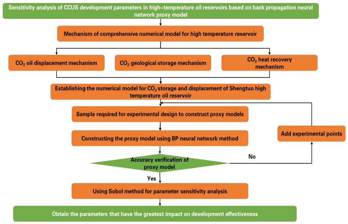
In the sensitivity parameter analysis of CO₂ capture, utilization, and storage (CCUS) in high-temperature oil reservoirs, it is necessary to repeatedly call numerical simulators (e.g., Eclipse, CMG) to simulate and obtain parameters that affect the effectiveness of CCUS development. However, manual parameter setting is cumbersome and labor-intensive, as it can only assess the impact of individual reservoir parameters in isolation. This process is time-consuming, often taking several months to complete. Thus, identifying the reservoir parameters most sensitive to CCUS development effectiveness and providing guiding suggestions for parameter adjustment have become urgent issues to address. In this study, a proxy model was constructed based on a backpropagation neural network, which was trained using data from the comprehensive numerical model of CCUS in high-temperature oil reservoirs. The Sobol global sensitivity analysis method was then employed to evaluate the impacts of different reservoir parameters on oil recovery rate, CO₂ geological storage capacity, and CO₂ heat recovery. The overall workflow is illustrated in Figure 1.

2. Research on the Mechanism of Numerical Models

2.1. CO₂ Oil Displacement Mechanism

Miscible and immiscible displacement mechanisms are the most common types of CO₂ displacement technologies in oil recovery and geological storage. The immiscible oil displacement mechanism mainly involves the following five aspects: (1) Dissolving CO₂ into oil reduces the oil’s viscosity, thereby enhancing its fluidity, expanding the oil volume, and increasing formation energy. (2) It improves the mobility ratio of oil to water, reduces the interfacial tension between oil and water, and enhances the displacement efficiency of CO₂. (3) During the injection of CO₂ into the reservoir, the formation pressure continues to rise, leading to increasing CO₂ dissolution in the oil. After stopping CO₂ injection, continuous extraction of formation oil causes a pressure drop, and the dissolved CO₂ in the oil escapes, forming a dissolved gas drive to promote oil displacement. (4) It improves formation permeability: CO₂ dissolved in formation water generates HCO₃⁻ and H⁺, which dissolve rock minerals in pore spaces and increase formation permeability. (5) It exerts a plugging removal effect, which can dissolve some blockages near the wellbore, playing a key role in unblocking the reservoir [26,27,28]. In contrast, the miscible displacement mechanism refers to the transition of CO₂ and formation oil from a two-phase fluid to a single-phase fluid under high temperature and pressure conditions. As a result, the interfacial tension between oil and CO₂ is close to zero, the capillary force between the two phases and the rock porous medium is reduced, and the flow resistance of oil is significantly decreased—ultimately enabling more oil to be extracted from the formation. The miscible displacement effect is significantly superior to that of immiscible displacement [29,30].

2.2. CO₂ Geological Storage Mechanism

Currently, scholars generally concur that oil and gas reservoirs are the most suitable sites for CO₂ geological sequestration. This suitability is primarily attributed to three key advantages: (1) During the exploration and development of oil and gas reservoirs, extensive and rigorous geological characterization has been conducted—encompassing storage capacity and cap-rock sealing efficiency—which effectively verifies the safety of CO₂ sequestration. (2) Existing surface and subsurface infrastructure (e.g., injection wells and supporting pipelines) can be repurposed for CO₂ geological sequestration, eliminating the need for full infrastructure reconstruction or requiring only partial upgrades. (3) CO₂-enhanced oil recovery (CO₂-EOR), which involves injecting CO₂ into oil and gas reservoirs to improve oil recovery, is a well-established practice in the oil and gas industry, with abundant on-site operational experience [31,32].

(1) Constructing storage mechanism

As a gaseous substance, CO₂ will migrate upward and accumulate beneath the impermeable cap rock once injected into the reservoir. In this process, CO₂ exists in the form of a high-density free phase and cannot penetrate the pore spaces of the cap rock, except through slow molecular diffusion [33].

(2) Dissolution storage mechanism

CO₂ dissolves readily in formation water, which reduces the volume of free-phase CO₂ within oil and gas reservoirs. The dissolution of CO₂ increases the density of formation water, causing it to migrate gradually toward the bottom of the formation under gravity; this process in turn accelerates the dissolution rate of injected CO₂ in formation water. Among all storage mechanisms, CO₂ dissolution offers the largest storage capacity, with a long-term stability of hundreds to thousands of years. Its safety is second only to mineral sequestration [31].

(3) Residual gas storage mechanism

After CO₂ is injected into the formation, it displaces water molecules within the rock pores during its migration. Due to differences in wettability and capillary forces, CO₂ is unable to pass through narrow, bottleneck-like pore throats and thus becomes trapped as residual gas. Residual trapping—a relatively stable physical storage mechanism—can persist for decades post-injection, making it safer than structural trapping. Residual trapping primarily occurs at the microscale and only takes full effect when groundwater re-infiltrates the pore spaces originally occupied by CO₂. Over time, the CO₂ trapped in the rock pores will gradually dissolve into the formation fluid, with the residual trapping mechanism typically maintaining its stability for several decades [34].

(4) Mineral storage mechanism

Mineral storage describes the process whereby bicarbonate (HCO₃⁻) and carbonate (CO₃²⁻) ions—generated from the hydrolysis of CO₂ dissolved in formation water—chemically react with calcium (Ca²⁺) and magnesium (Mg²⁺) ions released from rock-forming minerals, forming stable carbonate precipitates. Over geological time scales, these precipitates evolve into persistent carbonate minerals, enabling permanent carbon sequestration. Mineral trapping is primarily governed by geochemical reactions between rock minerals and formation fluids. Regarded as the safest and most reliable sequestration mechanism, mineral trapping typically persists for thousands to tens of thousands of years.

2.3. CO₂ Heat Production Mechanism

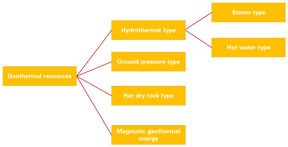
Geothermal resources are generally classified into four categories: hot dry rock, magmatic, geopressured, and hydrothermal types (Figure 2). Hot-dry-rock geothermal systems occur in water-poor subsurface formations, with temperatures ranging from 150 °C to 650 °C. Magmatic geothermal resources store massive thermal energy within molten and partially molten magma; they occur at the greatest depths and feature temperatures between 600 °C and 1500 °C. Geopressured geothermal resources exist in sedimentary basins, confined within high-pressure pore water at depths of 2000–3000 m and sealed by low-permeability shale. Their formation temperature ranges from 90 °C to 200 °C, and formation pressure can be several to over ten times hydrostatic pressure (30–100 MPa or higher). Beyond thermal energy, geopressured systems commonly contain chemical energy (e.g., methane) and high-pressure-driven mechanical energy, representing substantial energy potential. Hydrothermal geothermal resources, the most widely exploited type, are hosted in subsurface reservoirs with abundant thermal energy and are further categorized into vapor-dominated and hot-water-dominated systems based on their occurrence forms. Geothermal resources within high-temperature oil reservoirs fall into the hydrothermal category. During conventional reservoir production, most subsurface hot-water geothermal resources remain undeveloped, leading to considerable resource waste [35,36,37].

Two primary strategies exist for exploiting subsurface hot-water geothermal resources. The first involves direct extraction of hot formation water followed by surface treatment and utilization; nevertheless, this approach suffers from low extraction efficiency and may induce geothermal reservoir depletion, potentially triggering severe geological hazards such as seismic activity. The second strategy relies on injecting non-condensable gases (e.g., CO₂) into subsurface formations to recover geothermal hot water. When the temperature exceeds 31.1 °C and pressure surpasses 7.38 MPa, CO₂ enters a supercritical state, whose distinctive thermal properties confer superior heat-carrying performance. First, supercritical CO₂ exhibits density and viscosity values intermediate between those of liquid and gaseous phases, with a mass heat capacity 0.3–1.0 times that of water. According to Darcy’s law, under identical injection-production pressure drawdowns, its mass flow rate can be 1–6 times higher than water, yielding a heat recovery rate 1.4–2.7 times greater than that of water. Consequently, supercritical CO₂ possesses better injectivity and formation-infiltration capacity compared with water. Second, its thermal properties are highly sensitive to temperature and pressure variations. Under the same injection-production temperature difference, CO₂ undergoes more significant density changes than water, generating a stronger thermosiphon effect between injection and production wells. This effect provides natural driving pressure for surface facilities and reduces the power consumption of injection-production pumps. Third, supercritical CO₂ exerts minimal physicochemical interactions with rock-forming minerals. By fully replacing water as the heat-transfer medium, it effectively mitigates scaling issues within wellbores, pipelines and surface equipment, as well as environmental pollution arising from trace harmful mineral leaching [38].

In order to characterize the heat recovery capacity of CO₂ as the heat-carrying medium, the heat recovery capacity of CO₂ is defined as $Q$. The calculation formula is:

$$Q={\displaystyle \sum _{n=1}^N{\displaystyle {\int }_0^{{\mathrm{t}}_{end}}{q}_i\cdot C_P\cdot }\left(t_{out}-t_{in}\right)\mathrm{dt}}$$

(1)

In the formula, $Q$ represents the cumulative heat recovery of CO₂, J; $N$ represents the total number of production wells; $q_i$ represents the production rate of the i-th production well, kg/s; $C_P$ represents the specific heat capacity of the heat-carrying medium, $\mathrm{J}/(\mathrm{kg}\cdot \mathrm{K})$; $t_{out}$ represents the temperature of the produced fluid, K; and $t_{in}$ represents the temperature of the injected fluid, K.

3. Comprehensive Numerical Mode

3.1. Divide the Numerical Model Grid

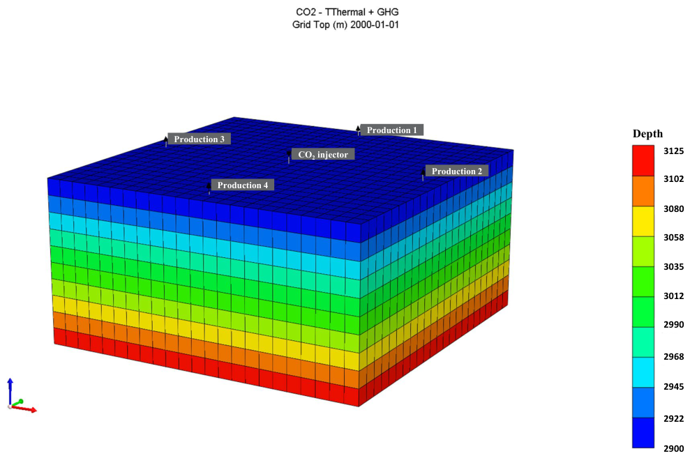
The Shengtuo Oil Reservoir is a typical high-temperature bottom-water reservoir. Using the CMG numerical simulation platform (CMG 2024.2), a comprehensive reservoir model was constructed that incorporates CO₂ miscible flooding, geological sequestration, and thermal recovery mechanisms. An inverted five-spot well pattern was adopted, consisting of five vertical wells: one central injector and four surrounding producers. The model employs corner-point grids with a total grid number of 23 × 23 × 10 = 3703, corresponding to the reservoir domain of 180 m × 180 m × 22 m. The formation is vertically divided into oil-bearing zones and bottom-water zones, where the upper four layers represent oil zones and the lower three layers are hot-water aquifers. The well-location layout is illustrated in Figure 3.

3.2. Basic Parameters of Numerical Model

The reservoir numerical model was configured with a porosity of 0.28 and a permeability of 89 × 10⁻³ μm². The reservoir is unfaulted and unfractured, with a burial depth of 2900 m and a formation temperature of 98 °C. Under reservoir conditions, the diffusion coefficient of CO₂ in formation water is approximately 12.9 × 10⁻⁹ m²/s, and the CO₂ injection temperature is set to 30 °C. To maintain injection-production balance, the CO₂ injection rate and liquid production rate were both fixed at 14,000 m³/d. The simulation duration was set to 40 years for CO₂ displacement and 260 years for long-term CO₂ sequestration.

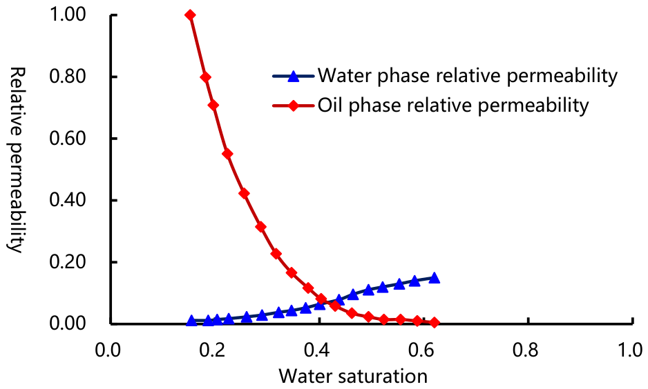
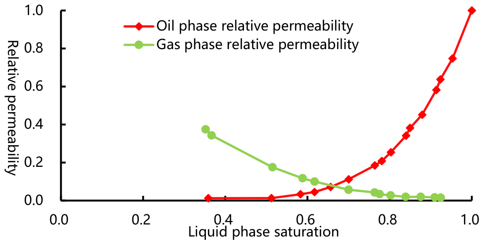
The fluid properties in the model were derived from experimental data of formation fluids in the Shengtuo Oil Reservoir. The reservoir’s initial water saturation is 0.39, with the oil having an average viscosity of 3.86 mPa·s, a density of approximately 0.881 g/cm³, and a relative molecular weight of 183.55. The oil–water and oil–gas relative permeability curves are presented in Figure 4 and Figure 5, respectively.

3.3. Research on the Influencing Factors of CCUS Development

Key parameters governing the CCUS performance of high-temperature oil reservoirs can be categorized into reservoir geological parameters and dynamic development parameters. Geological parameters are primarily dominated by reservoir heterogeneity, commonly characterized by rhythmic variations in permeability. Dynamic development parameters mainly include the CO₂ injection rate, liquid production rate, and CO₂ injection purity. In this study, representative parameters, including permeability rhythm, CO₂ injection purity, CO₂ injection rate, and liquid production rate, were selected for single-factor sensitivity analysis. For single-factor analysis, all other parameters are kept constant, while only one parameter is varied to evaluate its individual influence on development performance.

3.3.1. Research on Reservoir Heterogeneity

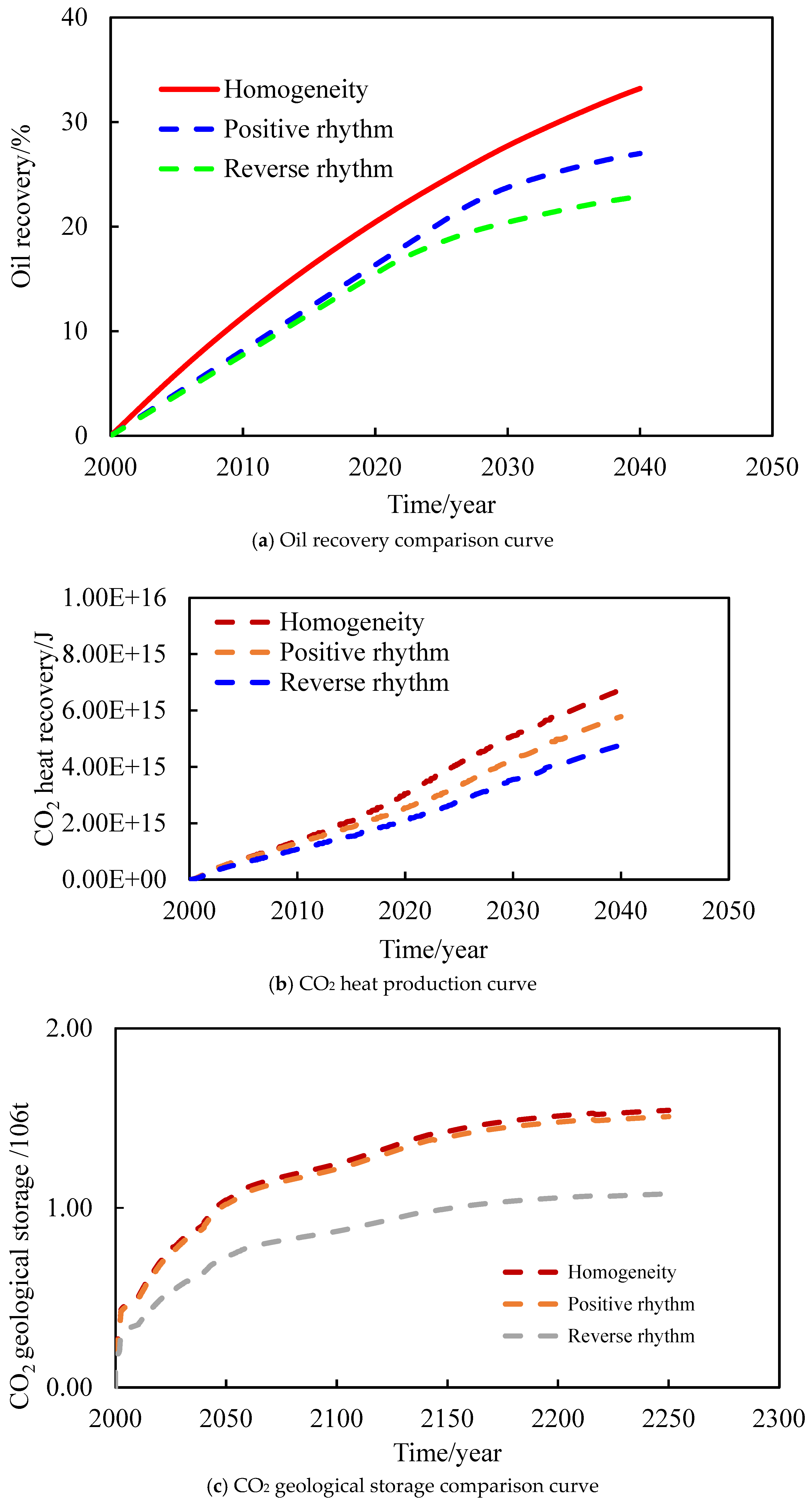
Permeability rhythm is the key parameter characterizing reservoir heterogeneity. Under the premise of maintaining a constant average permeability (89 × 10⁻³ μm²), the impacts of homogeneous permeability, positive rhythm, and negative rhythm on development performance were investigated separately.

Table 1. Development effect of different permeability rhythms.

Permeability Rhythm (Permeability Gradient Is 5)	Oil Recovery (%)	Heat Quantity (1015 J)	CO2 Dissolved Storage (106 t)	CO2 Structural Storage (106 t)	CO2 Residual Gas Storage (106 t)	CO2 Mineralized Storage (106 t)	Total Amount of CO2 Geological Storage (106 t)
Homogeneity	33.21	6.8	0.71	0.46	0.12	0.25	1.54
Positive rhythm	26.99	5.78	0.67	0.49	0.1	0.24	1.51
Reverse rhythm	23.84	4.83	0.5	0.26	0.078	0.24	1.08

presents a comparison of development performances under different permeability rhythms. Figure 6a shows the comparison curve of the oil recovery factor, Figure 6b shows the comparison curve of CO₂ heat recovery, and Figure 6c shows the comparison curve of CO₂ geological sequestration capacity.

Through the analysis of the results, it can be concluded that permeability rhythm exerts a significant impact on development performance. Specifically, the development effect of the homogeneous permeability reservoir model is superior to that of the positive and reverse rhythm models. The lowest oil recovery rate in the reverse rhythm model is mainly attributed to the uniform advancement of CO₂ toward production wells in homogeneous formations during injection, which effectively reduces the risk of gas channeling and thus achieves the highest CO₂ affected volume and efficiency. In contrast, the reverse rhythm model, characterized by high reservoir permeability, tends to experience CO₂ breakthrough through high-permeability zones during injection, leading to reduced CO₂ effectiveness and lower oil recovery rates. Additionally, the positive rhythm reservoir model outperforms the reverse rhythm model in terms of heat recovery and CO₂ geological sequestration capacity. This is primarily because the reservoir in question is a bottom-water reservoir; the positive rhythm model features higher permeability in the hot water layer compared to the reverse rhythm model, which directly contributes to improved CO₂ heat recovery and enhanced geological sequestration capacity.

3.3.2. Research on Developing Dynamic Parameters

1. Development effect of the purity of CO₂ injection gas

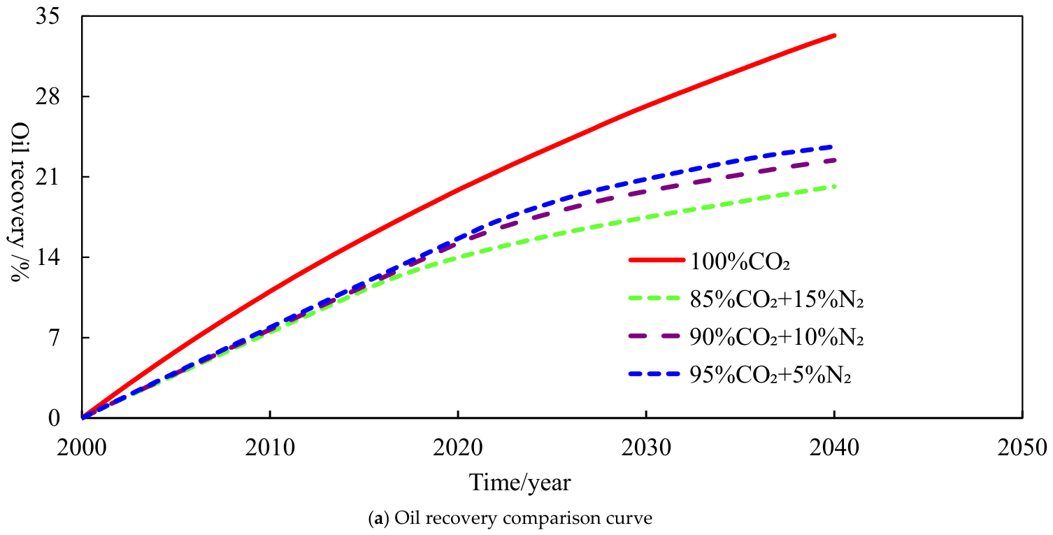
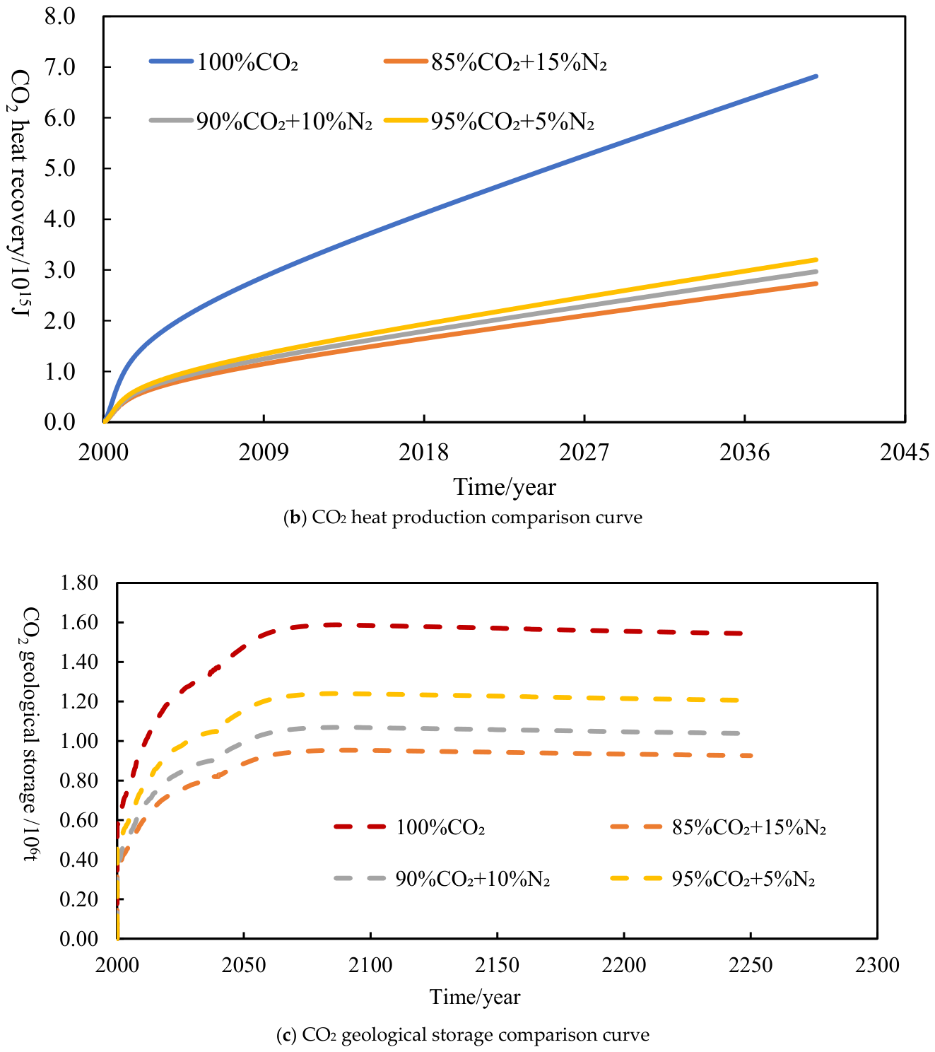
The numerical model considers the degree of influence on the development effect of CCUS under four conditions of CO₂ purity: 100%, 95% (5% N₂), 90% (10% N₂), and 85% (15% N₂).

Table 2. Development effect of different purity values of CO₂ injection gas.

Composition of Injected Gas (%)		Oil Recovery (%)	Heat Quantity (1015 J)	CO2 Dissolved Storage (106 t)	CO2 Structural Storage (106 t)	CO2 Residual Gas Storage (106 t)	CO2 Mineralized Storage (106 t)	Total Amount of CO2 Geological Storage (106 t)
CO2	N2
100	0	33.21	6.80	0.71	0.46	0.12	0.25	1.54
95	5	23.63	3.20	0.53	0.23	0.15	0.29	1.21
90	10	22.45	2.97	0.46	0.19	0.13	0.25	1.04
85	15	20.16	2.73	0.41	0.17	0.12	0.23	0.93

shows the comparison of development effects of different injection purities. Figure 7a shows the comparison of oil recovery under different CO₂ injection purities, Figure 7b shows the comparison of CO₂ heat recovery under different CO₂ injection purities, and Figure 7c shows the geological reserve of CO₂ under different CO₂ injection purities. Simulation analysis reveals that the purity of the injected CO₂ significantly impacts development performance. Impurity gases in the injected CO₂ can affect the miscibility between CO₂ and oil in the reservoir, thereby reducing the efficiency of CO₂ storage and displacement. Among the various impacts, oil recovery efficiency is the most affected, followed by heat recovery and CO₂ storage capacity. Specifically, the oil recovery rate for the 85% CO₂ injection purity is up to 9.58% lower than that of 100% CO₂ injection purity.

2. Development effects of different CO₂ gas injection rates

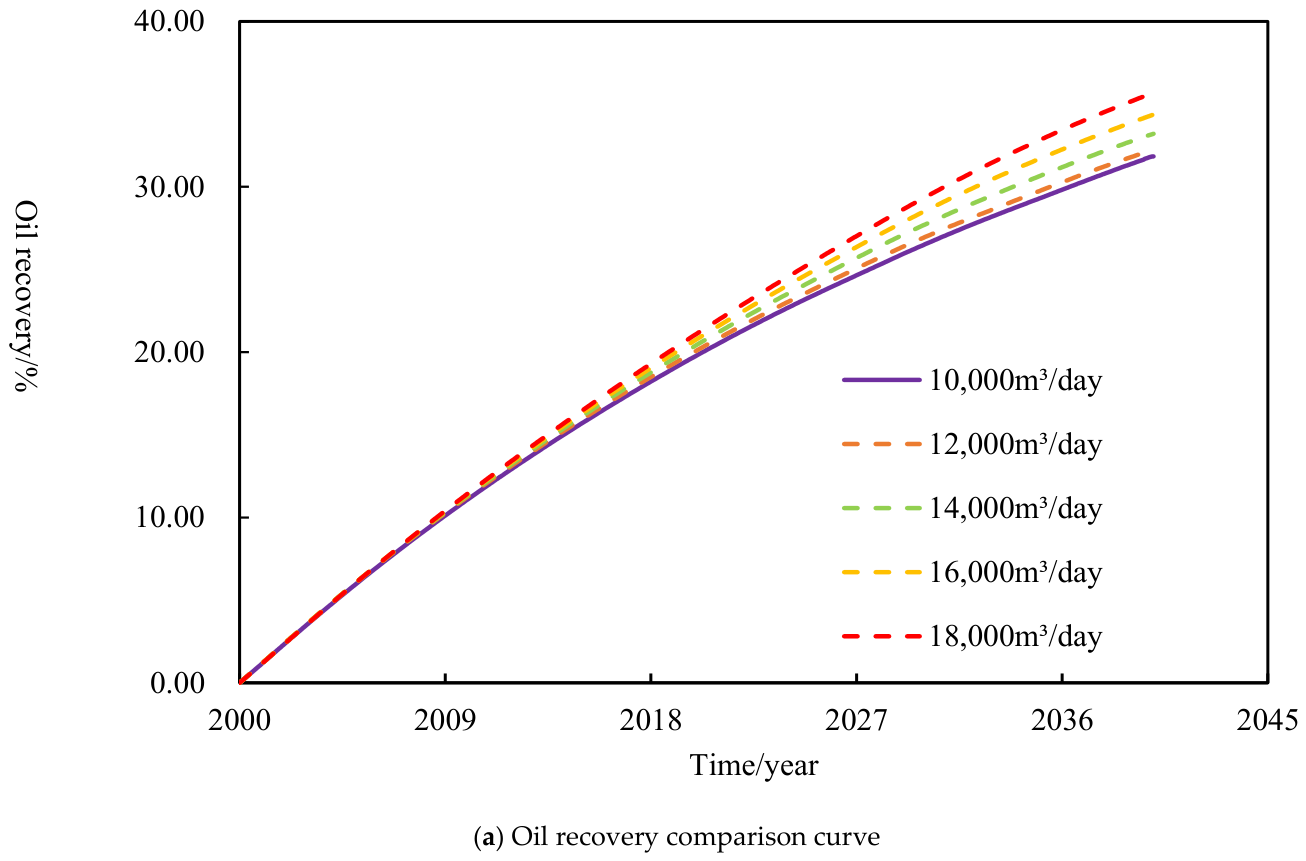
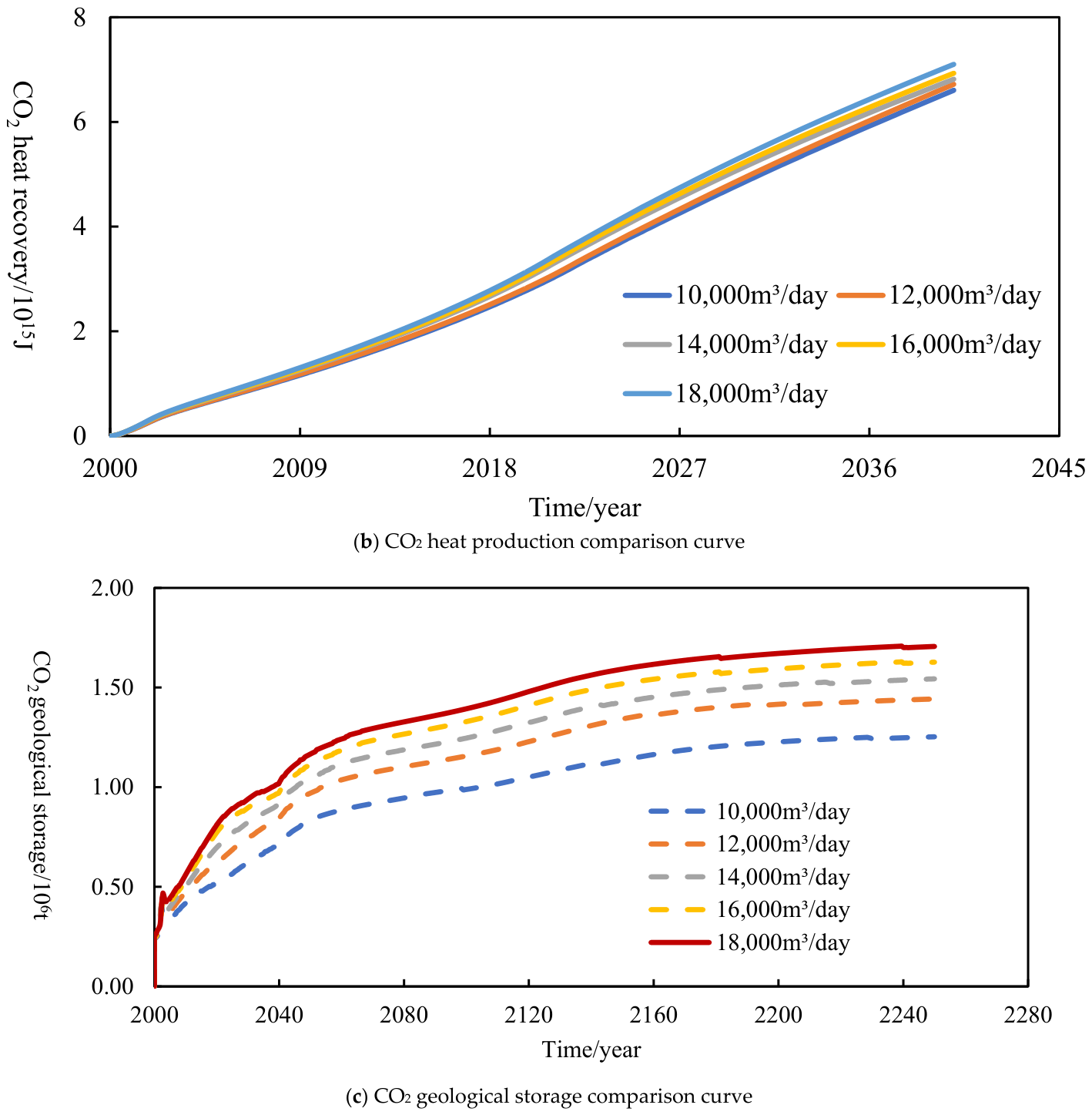
Five different gas injection rates are set: 10,000 m³/day, 12,000 m³/day, 14,000 m³/day, 16,000 m³/day and 18,000 m³/day. The effect of gas injection rate on reservoir development is studied.

Table 3. Development effects of different gas injection rates.

Gas Injection Rate (m3/Day)	Oil Recovery (%)	Heat Quantity (1015 J)	CO2 Dissolved Storage (106 t)	CO2 Structural Storage (106 t)	CO2 Residual Gas Storage (106 t)	CO2 Mineralized Storage (106 t)	Total Amount of CO2 Geological Storage (106 t)
10,000	31.84	6.6	0.57	0.4	0.098	0.18	1.25
12,000	32.24	6.7	0.65	0.44	0.11	0.24	1.44
14,000	33.21	6.80	0.71	0.46	0.12	0.25	1.54
16,000	34.37	6.9	0.79	0.48	0.13	0.26	1.66
18,000	35.69	7.1	0.85	0.49	0.14	0.27	1.75

shows a comparison of the development effects of different CO₂ gas injection rates. Figure 8a shows the comparison curve of oil recovery, Figure 8b shows the comparison curve of CO₂ heat recovery, and Figure 8c shows the comparison curve of CO₂ geological storage capacity. Result analysis reveals that both the oil recovery rate and CO₂ geological sequestration capacity increase with the rising CO₂ injection rate. However, the growth rate of the oil recovery rate is relatively modest, with a maximum increase of only 3.85%. This is primarily because an increase in the CO₂ injection rate enhances the likelihood of CO₂ breakthrough, which easily forms gas channeling through preferential seepage pathways. This phenomenon impairs the oil displacement efficiency of CO₂, resulting in a low growth rate of oil recovery. Similarly, CO₂ heat recovery increases with the CO₂ injection rate, but its growth is also relatively slight, with a maximum increment of only 0.5 × 10¹⁵ J. Notably, a higher CO₂ injection rate corresponds to a greater injected CO₂ volume and thus higher injection costs. Therefore, it is essential to comprehensively consider economic benefits and various development performances to determine the optimal CO₂ injection rate.

3. Development effects of different liquid production rates

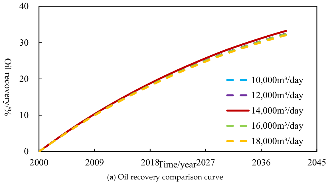
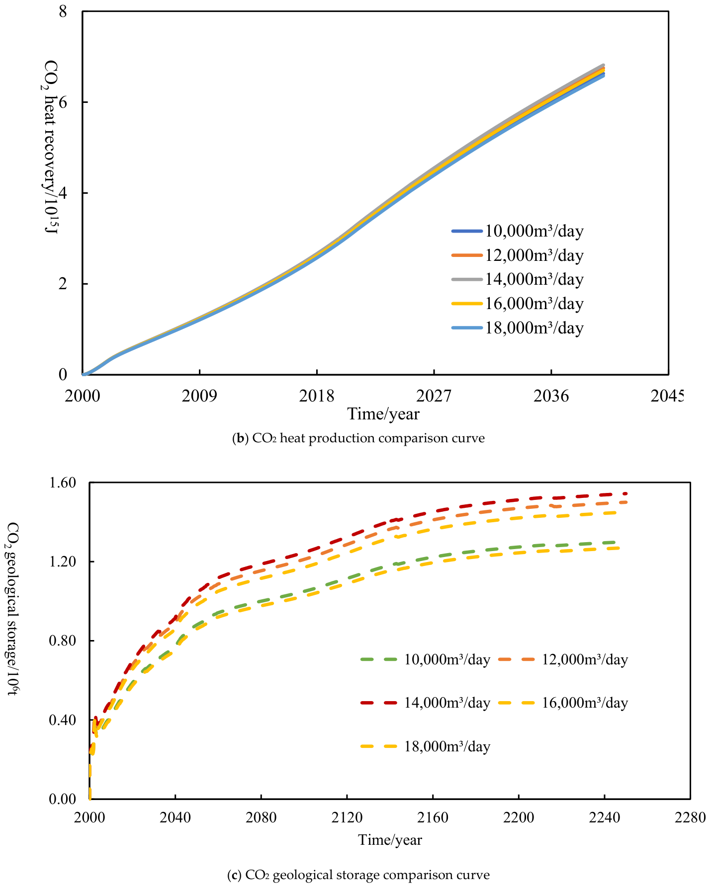
Five different liquid production rates are set: 10,000 m³/day, 12,000 m³/day, 14,000 m³/day, 16,000 m³/day and 18,000 m³/day. The effect of liquid production rate on reservoir development is studied.

Table 4. Development effects of different liquid production rates.

Liquid Production Rate (m3/Day)	Oil Recovery (%)	Heat Quantity (1015 J)	CO2 Dissolved Storage (106 t)	CO2 Structural Storage (106 t)	CO2 Residual Gas Storage (106 t)	CO2 Mineralized Storage (106 t)	Total Amount of CO2 Geological Storage (106 t)
10,000	32.13	6.63	0.59	0.42	0.10	0.19	1.30
12,000	32.45	6.75	0.68	0.46	0.11	0.25	1.50
14,000	33.21	6.80	0.71	0.46	0.12	0.25	1.54
16,000	32.35	6.70	0.69	0.42	0.11	0.23	1.45
18,000	32.02	6.58	0.62	0.36	0.10	0.20	1.27

shows a comparison of development effects of different liquid production rates. Figure 9a shows the comparison curve of oil recovery, Figure 9b shows the comparison curve of CO₂ heat recovery, and Figure 9c shows the comparison curve of CO₂ geological storage capacity.

Through result analysis, it was found that with the constant CO₂ injection rate, the oil recovery rate, CO₂ heat recovery, and CO₂ storage capacity all exhibit the trend of first increasing and then decreasing as the liquid extraction rate increases. When the liquid extraction rate is equal to the CO₂ injection rate (i.e., achieving injection-production balance), the oil recovery rate, CO₂ heat recovery, and CO₂ storage capacity reach their maximum values.

The primary reason for this phenomenon is that the liquid extraction rate is lower than the CO₂ injection rate; therefore, the injected CO₂ cannot be fully dissolved and utilized, leading to gas channeling and reduced displacement efficiency. Conversely, when the liquid extraction rate is higher than the CO₂ injection rate, the formation pressure drops significantly, resulting in insufficient formation energy to drive CO₂ dissolution and heat transfer, thereby reducing the CO₂ storage capacity and heat recovery. Only when the liquid extraction rate matches the CO₂ injection rate can the injected CO₂ be fully dissolved and utilized, maximizing the development effect and CO₂ storage efficiency.

As demonstrated in the above analysis, single-factor sensitivity analysis only evaluates performance variations under limited discrete changes of individual parameters, which lacks representativeness. In addition, manual parameter adjustment is computationally cumbersome and fails to cover all potential values of influencing factors. Accordingly, this study integrates a proxy model with a global sensitivity analysis approach to perform multi-parameter sensitivity evaluation, so as to quantify the relative influence of each parameter on overall development performance.

4. Parameter Sensitivity Analysis

4.1. Proxy Model

The proxy model refers to the mathematical model constructed from a limited number of experimental samples that maintains acceptable accuracy while featuring low computational complexity and high computational efficiency, with predicted outputs consistent with those from the target complex system. For sensitivity analysis of CCUS development parameters in high-temperature oil reservoirs, complex numerical simulation systems are typically required. Repeatedly running such numerical simulations is highly time-consuming and computationally intensive. Consequently, proxy models are adopted to approximate calculations performed by the original numerical simulator for sensitivity analysis, significantly improving computational efficiency. Among the mainstream surrogate model approaches widely applied in reservoir engineering, backpropagation (BP) neural networks, radial-basis-function (RBF) interpolation, and Kriging interpolation are the most commonly used.

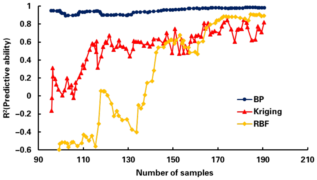
From Figure 10, it can be observed that the performance indicators of different proxy models tend to stabilize when the dataset size is 170. To comprehensively evaluate the accuracy and precision of the prediction results from different proxy model methods, under the premise of a unified dataset size of 170, parameters such as the coefficient of determination squared (R²), average absolute percentage relative error (AAPRE), average percentage relative error (APRE), root mean squared error (RMSE), and standard deviation (SD) were used to conduct a comprehensive error study on different methods. The results obtained are presented in

Table 5. Comparison of statistical errors of different proxy model methods.

Methods	R2	AAPRE (%)	APRE (%)	RMSE (%)	SD (%)
BP	0.985	2.060	0.083	0.655	0.053
RBF	0.813	13.57	0.29	3.68	0.21
Kriging	0.675	19.61	6.67	7.71	0.39

. From Figure 10 and Table 5, it can be seen that previous analyses have shown that Kriging dependent samples have significantly more features than radial basis function (RBF), and there is a certain degree of oscillation. The predictive ability of radial basis function interpolation is extremely unstable, while the BP neural network relies on a small number of samples, high accuracy, fast convergence, and stable and reliable results. Therefore, this method is chosen to construct the proxy model for sensitivity analysis.

Following the construction of the reservoir geological model, the adjustment ranges of uncertain reservoir parameters are determined via uncertainty analysis. Subsequently, experimental design is implemented for the target reservoir parameters, and the corresponding response variables are calculated using a reservoir numerical simulator. Finally, target response values are established based on the computed response variables and field-observed data.

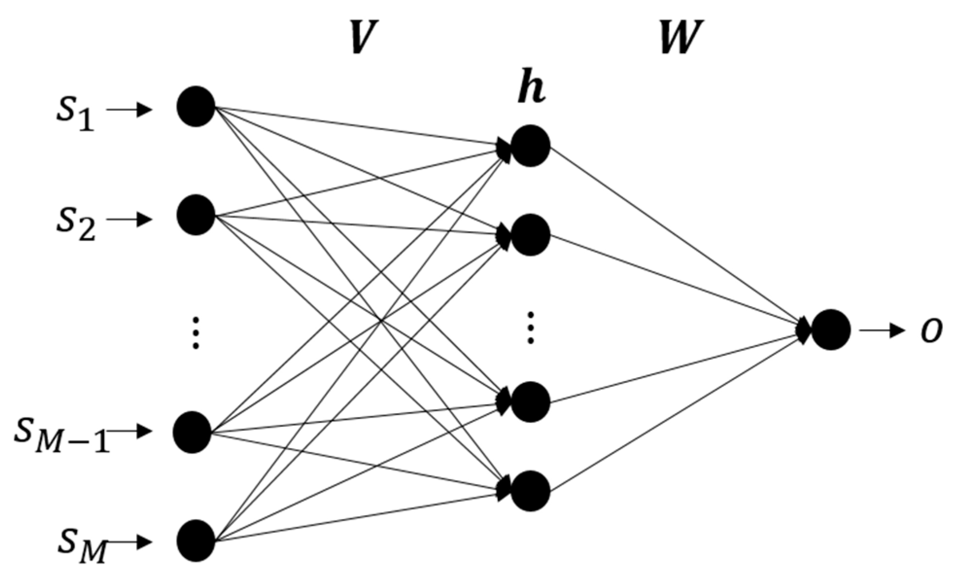
The supervised-learning-based improved backpropagation (BP) neural network adopts a three-layer architecture: an input layer, a hidden layer, and an output layer. The hidden layer may contain one or more layers of neural nodes, as illustrated in Figure 11. Information propagates from the input layer to the output layer through connection weights between adjacent layers, which are iteratively optimized via supervised-learning training algorithms. As a widely used machine learning technique, the BP neural network provides a robust learning framework characterized by a simple structure and convenient implementation. Given training samples, it can construct high-accuracy nonlinear mappings by means of effective supervised-learning algorithms [39].

(1) Multi-layer perceptron mathematical model

In the three-layer perceptron shown in Figure 11, the input vector is $\mathit{s}=\left[s_1,s_2,\dots ,s_M\right]$, the output vector of the hidden layer is $\mathit{h}=\left[h_1,h_2,\dots ,h_K\right]$, the output vector of the output layer is $\mathit{o}=\left[o_1,o_2,\dots ,o_L\right]$, and the expected output is $\mathit{y}=\left[y_1,y_2,\dots ,y_L\right]$. In the study, the response output is the historical fitting error value, which is a scalar data, so L = 1. The weight matrix from the output layer to the hidden layer is represented by V ($\mathit{V}=\left[{\mathit{V}}_1,{\mathit{V}}_2,\dots ,{\mathit{V}}_K\right])$, where the column vector V_j represents the weight vector corresponding to the j-th neuron in the hidden layer. The weight matrix between the hidden layer and the output layer is represented by W ($\mathit{W}=\left[{\mathit{W}}_1,{\mathit{W}}_2,\dots ,{\mathit{W}}_L\right])$, where the column vector W_k represents the weight vector corresponding to the kth neuron in the output layer.

For the output layer:

$$o_k=f\left({net}_k\right) k=1,2,\dots ,L$$

(2)

$${net}_k={\displaystyle {\sum }_{j=0}^K}{\omega }_{jk}{h}_j k=1,2,\dots ,L$$

(3)

For the hidden layer:

$$h_j=f\left({net}_j\right) j=1,2,\dots ,K$$

(4)

$${net}_j={\displaystyle {\sum }_{i=0}^M}{v}_{ij}{s}_i j=1,2,\dots ,K$$

(5)

Here, S₀ and h₀ are set to introduce thresholds for the hidden layer and output layer neurons, where S₀ = −1 and h₀ = −1. In Equation (6), the type of transformation function f(x) is a unipolar Sigmoid function.

$$f\left(x\right)={\displaystyle \frac{1}{1+e^{-x}}}$$

(6)

$f\left(x\right)$ has the characteristics of continuity and differentiability, and satisfies

$$f^{\prime }\left(x\right)=f\left(x\right)\left[1-f\left(x\right)\right]$$

(7)

According to the specific application needs, bipolar Sigmoid functions can also be used.

$$f\left(x\right)={\displaystyle \frac{1-e^{-x}}{1+e^{-x}}}$$

(8)

Equations (2)–(8) together form the mathematical model of a three-layer perceptron.

(2) Network Error and Weight Adjustment

The network output built on the multi-layer perceptron model is not equal to the actual expected output. The error between the two is defined as E, expressed as follows:

$$E={\displaystyle \frac{1}{2}}{\left(\mathit{Y}-\mathit{O}\right)}^2$$

$$={\displaystyle \frac{1}{2}}{\displaystyle {\sum }_{k=1}^L}{\left(y_k-o_k\right)}^2$$

(9)

Expanding the above error definition formula to the hidden layer,

$$E={\displaystyle \frac{1}{2}}{\displaystyle \sum _{k=1}^L}{\left[y_k-f\left({net}_k\right)\right]}^2$$

$$={\displaystyle \frac{1}{2}}{\displaystyle {\sum }_{k=1}^L}{\left[y_k-f\left({\displaystyle {\sum }_{j=0}^K}{\omega }_{jk}{h}_j\right)\right]}^2$$

(10)

Further expanding Equation (10) to the output layer,

$$E={\displaystyle \frac{1}{2}}{\displaystyle \sum _{k=1}^L}{\left\{y_k-f\left[{\displaystyle \sum _{j=0}^K}{\omega }_{jk}f\left({net}_j\right)\right]\right\}}^2$$

$$={\displaystyle \frac{1}{2}}{\displaystyle {\sum }_{k=1}^L}{\left\{y_k-f\left[{\displaystyle {\sum }_{j=0}^K}{\omega }_{jk}f\left({\displaystyle {\sum }_{i=0}^M}{v}_{ij}{s}_i\right)\right]\right\}}^2$$

(11)

From Equation (11), it can be seen that the network output error E is a function of the weights ω_jk and v_ij, so the network output error can be reduced by continuously adjusting the weights. Obviously, the principle of adjusting weights in this process is to keep the output error E decreasing, which is a typical optimization method. The objective function is the output error, and the optimization parameter vector is the weight vector. The BP algorithm is characterized by the forward calculation of information and the backpropagation of error. Weight adjustment occurs during the process of repeated signal flow direction, and the adjustment amplitude is proportional to the gradient decline of the error; that is,

$$\Delta {\omega }_{jk}=-\eta {\displaystyle \frac{\partial E}{\partial {\omega }_{jk}}} j=0,1,2,\dots ,K;k=1,2,\dots ,L$$

(12)

$$\Delta v_{ij}=-\eta {\displaystyle \frac{\partial E}{\partial v_{ij}}} i=0,1,2,\dots ,M;j=1,2,\dots ,K$$

(13)

In the equation, the number $\eta \in \left(0,1\right)$ represents the proportional coefficient, which represents the rate of weight adjustment during neural network training. The standard BP algorithm, which uses the steepest descent method to train a network, usually has the disadvantages of slow convergence speed and is prone to falling into local optima. For the same experimental dataset $\mathit{S}={[{\mathit{s}}_{\mathbf{1}}\cdots {\mathit{s}}_{\mathit{N}}]}^T$ and response value $\mathit{Y}={[y_1\cdots y_N]}^T$, an improved algorithm, Levenberg–Marquardt, is used to train the network. The LM algorithm combines the advantages of the gradient method and Newton’s method, and the value of the damping coefficient λ can achieve step size adjustment for both methods.

(3) Design of Multi-Layer Perceptron Structure

The selection and calculation of initial weights, the number of hidden layer nodes, and incentive functions for the network are determined using the improved method proposed in reference [39].

(4) Parameter Design of BP Neural Network

Network structure: A single hidden layer is adopted, with the number of neurons in the hidden layer determined to be 12 through trial calculations. The number of neurons in the input layer is consistent with the dimension of the input variables, and the number of neurons in the output layer is 1. The activation function for the input and hidden layers is selected as the Sigmoid function, while the output layer adopts a linear activation function.

Hyperparameter settings: The learning rate is set to 0.01, gradient descent is used for weight updates, the maximum number of iterations is set to 1000, and the target convergence error is 1 × 10⁻⁴.

Data partitioning: A random partitioning approach is adopted, with 80% of the samples serving as the training set for model training and 20% as the test set for model performance validation. A fixed random seed is set during the partitioning process to ensure reproducibility of the data partitioning.

4.2. Sensitivity Analysis

4.2.1. Analysis Method

As elaborated in Section 2.3, conventional sensitivity analysis based on manually predefined parameters generally assesses the impact of only one development parameter on production performance at a time. Such a method cannot identify the dominant parameters controlling reservoir performance under multi-parameter coupling conditions and is also plagued by excessive time consumption, high labor costs, and heavy computational loads. For reservoir numerical simulations representing complex and strongly nonlinear systems, global sensitivity analysis provides more reliable results. By evaluating responses over the full parameter space, this method allows qualitative evaluation and quantitative measurement of both individual and interactive effects of multiple parameters on model outputs.

Table 6. Global sensitivity analysis method.

Methods	Characteristic
multivariate regressive method	Based on the Latin hypercube sampling method, the sensitivity of each parameter is represented using the multiple linear regression coefficients or partial correlation coefficients of the sampled data.
Morris	Comparing the calculation results of adjacent parameters in the parameter space, quantization sorting is simple and effective, but the overall efficiency is low.
RSA	Taking into account the complexity and correlation of research parameters, it visualizes the important parameters in the simulation process and quantify their sensitivity.
GLUE	Combining RSA and fuzzy mathematics theory, it provides quantitative sensitivity analysis results of parameters in the form of scatter plots.
Sobol	Based on Monte Carlo sampling and variance decomposition theory, the sensitivity of model parameters to multiple orders can be analyzed, and the impact of multiple parameters on the output results can be considered simultaneously, providing quantitative results.

summarizes several widely used global sensitivity analysis methods together with their key features.

Among all the global sensitivity analysis methods mentioned above, the Sobol method is a highly representative global sensitivity row analysis method that is based on the idea of variance decomposition and can obtain sensitivity values of parameters 1, 2, and higher orders [40].

The Sobol method was first proposed in 1993. Its main idea is to decompose the function $f\left(\mathit{x}\right),\mathit{x}\in R_n$ into the sum of 2ⁿ increasing terms, and calculate the total variance and partial variance of the model response through Monte Carlo sampling, in order to obtain the corresponding sensitivity. Assuming that the model is $y=f\left(\mathit{x}\right)$, x_i follows a uniform distribution of [0, 1], and $f^2\left(\mathit{x}\right)$ is integrable, the model can be decomposed into

$$f\left(\mathit{x}\right)=f_0+{\displaystyle {\sum }_{i=1}^n}{f}_i\left(x_i\right)+{\sum }_{\begin{array}{c}i,j=1,2,\cdots ,n\\ i<j\end{array}}{f}_{i,j}\left(x_i,x_j\right)+\cdots +f_{1,2,\cdots ,n}\left(x_1,x_2,\cdots ,x_n\right)$$

(14)

The total variance of the model can also be decomposed into independent parameters and the interactive effects between different parameters.

$$D={\displaystyle {\sum }_{i=1}^n}{D}_i+{\displaystyle {\sum }_{i=1}^n}{\displaystyle {\sum }_{\begin{array}{c}j=1\\ i\ne j\end{array}}^n}(D_{ij}+\cdots +D_{1,2,\cdots ,n})$$

(15)

Normalizing Equation (15) and $S_{i_1,\cdots ,i_n}={\displaystyle \frac{D_{i_1,\cdots ,i_n}}{D}}$, the sensitivity of individual parameters and the interaction between different parameters of the model can be obtained.

$$1={\displaystyle {\sum }_{i=1}^n}{S}_i+{\displaystyle {\sum }_{i=1}^n}{\displaystyle {\sum }_{\begin{array}{c}j=1\\ i\ne j\end{array}}^n}{S}_{ij}+\cdots +S_{1,2,\cdots ,n}$$

(16)

In the formula, $S_i$ is referred to as the first-order sensitivity, $S_{ij}$ is the second-order sensitivity, and according to this rule, $S_{1,2,\cdots ,n}$ is the nth-order sensitivity, with a total of $2^n-1$ sensitivity indices.

The Sobol method is adopted to conduct Monte Carlo sampling on the previously constructed proxy model and calculate global sensitivity indices of arbitrary order. Direct implementation using reservoir numerical simulations to guarantee sensitivity analysis accuracy would incur prohibitively high time costs for Monte Carlo sampling. The introduction of proxy models substantially reduces computational time, thereby enabling feasible global sensitivity analysis.

4.2.2. Set Sensitivity Parameters

From the results in Figure 10, it can be seen that when the sample size reaches 170, the R² coefficient of the BP neural network model has reached a satisfactory level, and the sensitivity analysis results at this time can be considered to be true and reliable. With the goal of improving efficiency, sensitivity analysis is conducted on the proxy model established with a small sample size, and different sensitivity analysis results are compared. In sensitivity analysis, there may be certain differences in the types and ranges of development parameters. This depends on multiple factors, including reservoir geological conditions, development performance analysis, and the degree to which the objective function is controlled by various factors.

Based on the analysis of influencing factors in the development, these 7 parameters cover the influencing factors that affect the development effect of CCUS in high-temperature oil reservoirs. The value ranges of different parameters are shown in

Table 7. The sensitivity parameters and the value range.

Parameters	Min	Max	Description
GIR (m3/day)	10,000	18,000	Gas injection rate of injection wells
LPR (m3/day)	10,000	18,000	Liquid production rate of production wells
CO2 purity (%)	90	100	/
CO2 injection temperature (°C)	25	30	/
Reservoir temperature (°C)	85	105	/
Reservoir heterogeneity (Kv/Kh)	0.1	0.8	Comparing the different permeability rhythms
f	0.5	1.0	Completion degree of perforation wellbore

. The objective functions are oil recovery, CO₂ heat recovery and CO₂ geological storage, to determine the degree of influence of different sensitive parameters on each objective function. The calculation time of directly using numerical models for sensitivity analysis and using proxy models was compared. The time required by the numerical model was 8967 min, while the time required by the proxy model was only 3650 min, which was only 40.7% of that of direct analysis, greatly saving the calculation time.

4.3. Result Analysis

According to the principle of the Sobol method and Equation (14), it can be known that the variance $D_{i_1,\cdots ,i_n}$ of each order can be obtained by decomposing the calculation equation:

$$D_{i_1,i_2,\dots ,i_n}= {\displaystyle {\int }_0^1\dots }{\displaystyle {\int }_0^1{f}_{i_1,i_2,\dots ,i_k}^2}\left(x_1,x_2,\dots ,x_k\right)d{x}_{i_1}\dots d{x}_{i_n}$$

(17)

The ratio of the variance of the decomposed bias to the total variance is the sensitivity, which is the degree of influence:

$$S_{i_1,\cdots ,i_n}={\displaystyle \frac{D_{i_1,\cdots ,i_n}}{D}}$$

(18)

In the formula, D represents the total variance, as shown in Equation (15). $S_{i_1,\cdots ,i_n}$ is used to quantitatively describe the degree of influence of s parameters acting together on the function f(x). The influence degrees of the combined action of seven parameters, such as the CO₂ injection rate and CO₂ injection purity, on the objective function were respectively considered. From Equation (18), the influence degrees of different parameters on different objective functions—oil recovery, CO₂ heat recovery and CO₂ geological storage—can be obtained.

1. Oil recovery rate

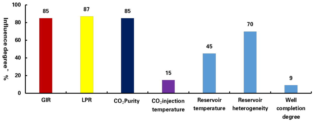
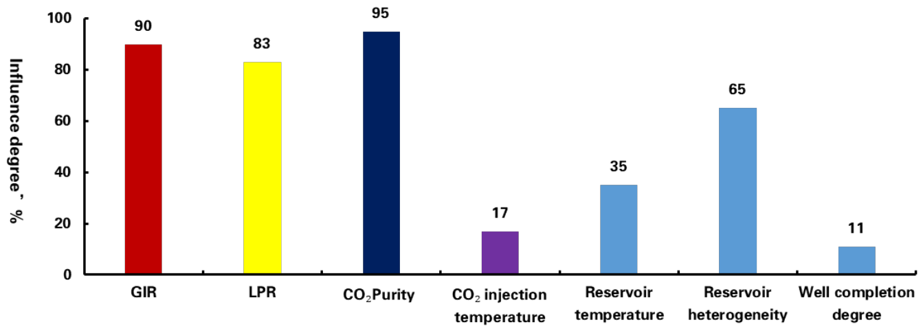
As illustrated in Figure 12, the parameters exerting the most significant influence on oil recovery (with an impact degree greater than 80%) are the CO₂ gas injection rate, liquid production rate, and CO₂ injection purity.

2. CO₂ heat recovery

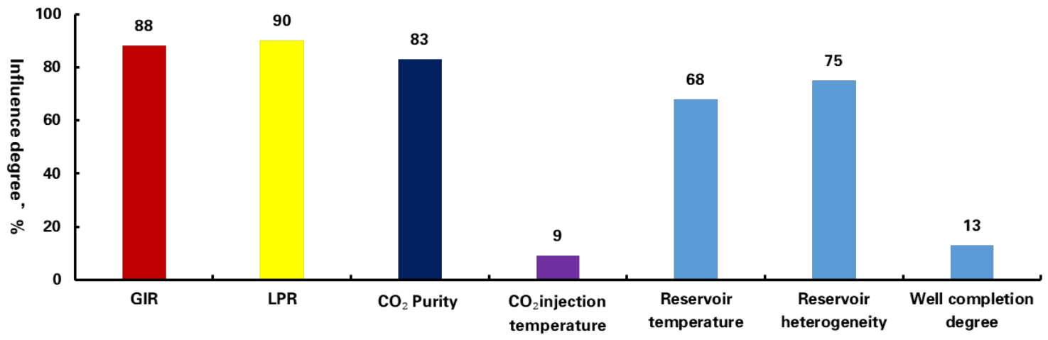
As can be seen from Figure 13, the parameters exerting the most significant influence on oil recovery (with an impact degree greater than 80%) are the CO₂ gas injection rate, liquid production rate, and CO₂ injection purity.

3. CO₂ geological storage

As can be seen from Figure 14, the parameters exerting the most significant influence on oil recovery (with an impact degree greater than 80%) are the CO₂ gas injection rate, liquid production rate, and CO₂ injection purity.

4. Error analysis

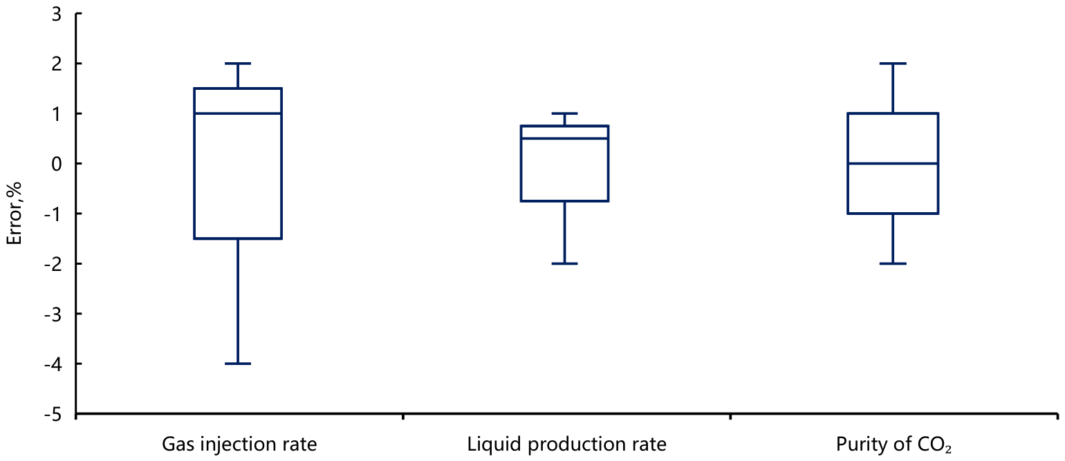
According to the degree of sensitivity, three parameters, namely the CO₂ injection rate, liquid production rate and CO₂ injection purity, were selected for analysis. The box plots of the variation errors from the sensitivity analysis of the development parameters under the proxy model are shown in Figure 15.

According to Figure 15, the experimental errors in the sensitivity analysis of developing parameters under the proxy model are all within ± 5%, which verifies the effectiveness and correctness of using the Sobol method for sensitivity analysis of the proxy model.

5. Conclusions

(1) Based on the actual geological data of the Shengtuo high-temperature oil reservoir, a comprehensive numerical model considering the CO₂ oil displacement mechanism, CO₂ heat recovery and CO₂ geological storage mechanism was established using numerical simulation software. A single factor analysis was conducted on the main parameters affecting the development effect.

(2) On the basis of the single factor analysis, a proxy model for the comprehensive numerical model of high-temperature oil reservoir CCUS was constructed using a BP neural network. The Sobol method was used to conduct sensitivity analysis on the development parameters that affect CO₂ displacement and storage in high-temperature oil reservoirs. Considering multiple parameters such as gas injection rate, liquid production rate, reservoir heterogeneity, and CO₂ injection purity, it was found that the gas injection rate, liquid production rate, and CO₂ injection purity exerted the most significant impacts on CCUS development performance. Additionally, an error analysis of the sensitivity results demonstrated that the errors for all considered parameters were within 5%, verifying the accuracy and effectiveness of the proposed approach.

(3) The proposed proxy model-based parameter sensitivity analysis method for CCUS development in high-temperature oil reservoirs can yield high-precision sensitivity results without relying on time-consuming numerical simulation calculations. This method reduces computational workload and time, effectively improving the efficiency of manual parameter adjustment, providing guidance for scheme optimization, and mitigating the blindness of parameter tuning. Furthermore, the established method can be extended to parameter sensitivity analysis in other fields of reservoir engineering.

References

1. Dumitrache, L.; Suditu, S.; Branoiu, G.; Neagu, D.; Alecu, M.D. Carbon Management and Storage for Oltenia: Tackling Romania’s Decarbonization Goals. Sustainability 2025, 17, 6793. [Google Scholar] [CrossRef] [Scilit]
2. Li, H.; Gong, C.; Liu, S.; Xu, J.; Imani, G. Machine learning-assisted prediction of oil production and CO2 storage effect in CO2-water-alternating-gas injection (CO2-WAG). Appl. Sci. 2022, 12, 10958. [Google Scholar] [CrossRef] [Scilit]
3. Meng, S.; Fu, Q.; Tao, J.; Liang, L.; Xu, J. Predicting CO2-EOR and storage in low-permeability reservoirs with deep learning-based surrogate flow models. Geoenergy Energy Sci. Eng. 2023, 233, 212467. [Google Scholar]
4. Dong, P.; Liao, X.; Zhang, L.; Zhang, H.; Zhao, X.; Xue, Q. A surrogate model for numericalreservoir simulation of CO2 flooding and storage based on deep learning. In Proceedings of the SPE/IATMI Asia Pacific Oil & Gas Conference and Exhibition, Jakarta, Indonesia, 10–12 October 2023. SPE-215253-MS. [Google Scholar]
5. Yao, P.; Yu, Z.; Zhang, Y.; Xu, T. Application of machine learning in carbon capture andstorage: An in-depth insight from the perspective of geoscience. Fuel 2023, 333, 126296. [Google Scholar] [CrossRef] [Scilit]
6. Zhao, Z. Radial Basis Function Surrogate Model Assisted Mechanical Structure Reliability Analysis and Design Optimization Method. Master’s Thesis, Hebei University of Technology, Tianjin, China, 2022. [Google Scholar]
7. Khan, W.A.; Rui, Z.; Hu, T.; Liu, Y.; Zhang, F.; Zhao, Y. Application of machine learning and optimization of oil recovery and CO2 sequestration in the tight oil reservoir. SPE J. 2024, 29, 2772–2792. [Google Scholar] [CrossRef] [Scilit]
8. Du, X.; Salasakar, S.; Thakur, G.C. A comprehensive summary of the application of machine learning techniques for CO2-EOR projects. Mach. Learn. Knowl. Extr. 2024, 6, 917–943. [Google Scholar] [CrossRef] [Scilit]
9. Yan, F.; Lu, H.; Yao, J.; Pei, X.; Feng, S.; Zhao, C. Optimizing interleaved distributed streamline obstacle flow channels through genetic algorithm coupled with backpropagation neural network regression predictive surrogate model. Fuel 2024, 372, 132174. [Google Scholar] [CrossRef] [Scilit]
10. Vaziri, P.; Sedaee, B. A machine learning-based approach to the multi-objective optimization of CO2 injection and water production during CCS in a saline aquifer based on field data. Energy Sci. Eng. 2023, 11, 1671–1687. [Google Scholar] [CrossRef] [Scilit]
11. Thanh, H.V.; Yasin, Q.; Al-Mudhafar, W.J.; Lee, K.-K. Knowledge-based machine learning techniques for accurate prediction of CO2 storage performance in underground saline aquifers. Appl. Energy 2022, 314, 118985. [Google Scholar] [CrossRef] [Scilit]
12. Mohaghegh, S.D.; Liu, J.; Gaskari, R.; Maysami, M.; Olukoko, O.A. Application of Surrogate Reservoir Model (SRM) to an Onshore Green Field in Saudi Arabia; Case Study. In Proceedings of the North Africa Technical Conference and Exhibition, Cairo, Egypt, 20–22 February 2012. SPE 151994. [Google Scholar]
13. Nassabeh, M.; You, Z.; Keshavarz, A.; Iglauer, S. Sub-surface geospatial intelligence in carbon capture, utilization and storage: A machine learning approach for offshore storage site selection. Energy 2024, 305, 132086. [Google Scholar] [CrossRef] [Scilit]
14. Sayyafzadeh, M. A Self-Adaptive Surrogate-Assisted Evolutionary Algorithm for Well Placement Optimization Problems. In Proceedings of the SPE/IATMI Asia Pacific Oil & Gas Conference and Exhibition, Nusa Dua, Bali, Indonesia, 20–22 October 2015. SPE 176468. [Google Scholar]
15. Artun, E.; Ertekin, T.; Waston, R.; Al-Wadhahi, M. Development of Universal Proxy Models for Screening and Optimization of Cyclic Pressure Pulsing in Narurally Fractured Reservoirs. In Proceedings of the IPTC 2009: International Petroleum Technology Conference, Doha, Qatar, 7–9 December 2009. [Google Scholar]
16. Liu, Y.; Chen, W.; Bao, Y.; Ding, L. Research on Fast and Robust Proxy model Based on Improved Support Vector Machine. Comput. Eng. Appl. 2015, 51, 7–11. [Google Scholar]
17. Moeinikia, F.; Alizadeh, N. Experimental Design in reservoir simulation: An integrated solution for uncertainty analysis, a case study. J. Pet. Explor. Prod. Technol. 2012, 2, 75–83. [Google Scholar] [CrossRef] [Scilit]
18. De Oliveira-De Jesus, P.M.; Sorrentino, E. A Monte Carlo method to solve the optimal coordination of directional overcurrent protections considering all the possible fault locations. Electr. Power Syst. Res. 2024, 236, 110974. [Google Scholar] [CrossRef] [Scilit]
19. Zhang, Q.; Li, Q.; Chen, Y.; Li, H.; Fan, S. A control method for wire stripping in distribution networks based on multiple linear regression. J. Electr. Power 2024, 39, 52–63. [Google Scholar]
20. Wang, D.; Mao, D.; Wang, Z.; Xiang, H.; Feng, K. Simulation of Land Cover Pattern Changes in Northeast China: Comparative Analysis Based on CLUE-S and Markov CA Models. Geogr. Sci. 2024, 44, 329–339. [Google Scholar]
21. García, A.; Negreanu, M.; Ureña, F.; Vargas, A. Numerical solution of a hydrodynamic model with cavitation using finite difference method at arbitrary meshes. Appl. Numer. Math. 2024, 205, 195–205. [Google Scholar] [CrossRef] [Scilit]
22. Liu, S.; Meng, X.; Yuan, Z.; Ren, L.; Chen, L. Optimization design of space radiation cooler based on response surface method and genetic algorithm. Case Stud. Therm. Eng. 2023, 50, 103437. [Google Scholar] [CrossRef] [Scilit]
23. Xu, B.; Wang, S.-D. Sensitivity analysis of factors affecting gravity dam anti-sliding stability along a foundation surface using Sobol method. Water Sci. Eng. 2023, 16, 399–407. [Google Scholar] [CrossRef] [Scilit]
24. Ren, Q.W.; Chen, Y.B.; Zhou, H.L.; Wang, B.D.; Wang, H.X. Global sensitivity analysis of TOPMODEL model based on Sobol method. People’s Yangtze River 2010, 41, 91–94+107. [Google Scholar]
25. Yao, Z.; Huang, C.; Duan, J.; Yu, H.; Chen, L. Evaluation Method for CO2 Displacement and Storage Potential in Extended Oilfield. J. Liaoning Univ. Petrochem. Technol. 2016, 36, 43–45. [Google Scholar]
26. Li, S.; Tang, Y.; Hou, C. Current Status and Development Trends of CO2 Injection Enhanced Oil Recovery Technology. Oil Gas Reserv. Eval. Dev. 2019, 9, 1–8. [Google Scholar]
27. Long, M.; Qi, G.; Feng, C. Research progress on carbon dioxide miscible and immiscible oil displacement technology. Sino Foreign Energy 2018, 23, 18–26. [Google Scholar]
28. Li, B. Study on CO2 Oil Displacement and Storage Effect in Sandstone Reservoirs. Master’s Thesis, Yanshan University, Qinhuangdao, China, 2016. [Google Scholar]
29. Hu, Y.; Hao, M.; Chen, G.; Sun, R.; Li, S. CO2 EOR and Storage Technology and Practice in China. Pet. Explor. Dev. 2019, 46, 716–727. [Google Scholar]
30. Chen, H. New progress in CO2 flooding and storage technology. Oil Gas Geol. Recovery 2023, 30, 18–26. [Google Scholar]
31. Silva, P.; Ranjith, P. A study of methodologies for CO2 storage capacity estimation of saline aquifers. Fuel 2012, 93, 13–27. [Google Scholar] [CrossRef] [Scilit]
32. Meng, Q.; Jiang, X. Numerical analyses of the solubility trapping of CO2 storage in geological formations. Appl. Energy 2014, 130, 581–591. [Google Scholar] [CrossRef] [Scilit]
33. Kneafsey, T.J.; Pruess, K. Laboratory flow experiments for visualizing carbon dioxide Induced, Density-Driven Brine Convection. Transp. Porous Media 2010, 82, 123–139. [Google Scholar] [CrossRef] [Scilit]
34. Bachu, S.; Gunter, W.; Perkins, E. Aquifer disposal of CO2: Hydrodynamic andmineral trapping. Energy Convers. Manag. 1994, 35, 269–279. [Google Scholar] [CrossRef] [Scilit]
35. Randolph, J.B. Coupling Geothermal Energy Capture with Carbon Dioxide Sequestration in Naturally Permeable, Porous Geologic Formations—A Novel Approach for Expanding Geothermal Energy Utilization. Ph.D. Thesis, University of Minnesota, Minneapolis, MN, USA, 2011. [Google Scholar]
36. Atrens, A.D.; Gurgenci, H.; Rudolph, V. Exergy analysis of a CO2 thermosiphon. In Proceedings of the Thirty-Fourth Workshop on Geothermal Reservoir Engineering, Stanford, CA, USA, 9–11 February 2009. [Google Scholar]
37. Remoroza, A.I.; Doroodchi, E.; Moghtaderi, B. CO2-EGS in hot dry rock: Preliminary results from CO2-rock interaction experiments. In Proceedings of the Thirty-Seventh Workshop on Geothermal Reservoir Engineering, Stanford, CA, USA, 30 January–1 February 2012. [Google Scholar]
38. Shi, H. Optimization Method for Injection Molding Warpage Based on Artificial Neural Network. Master’s Thesis, Dalian University of Technology, Dalian, China, 2012. [Google Scholar]
39. Sobol, I.M.; Kucherenko, S. A new derivative based importance criterion for groups of variables and its link with the global sensitivity indices. Comput. Phys. Commun. 2010, 181, 1212–1217. [Google Scholar] [CrossRef] [Scilit]
40. Sobol′, I.M. Global sensitivity indices for nonlinear mathematical models and their Monte Carlo estimates. Math. Comput. Simul. 2001, 55, 271–280. [Google Scholar] [CrossRef] [Scilit]
Figure 1. CCUS development parameter sensitivity analysis flowchart.
Energies 19 04117 g001
Figure 2. Classification of geothermal resource types.
Energies 19 04117 g002
Figure 3. Well location distribution in the comprehensive numerical model.
Energies 19 04117 g003
Figure 4. Oil–water relative permeability curve.
Energies 19 04117 g004
Figure 5. Oil and gas relative permeability curve.
Energies 19 04117 g005
Figure 6. Comparison of CCUS development effects under different permeability rhythms.
Energies 19 04117 g006
Figure 7. Comparison of CCUS development effects under different CO2 purity values.
Energies 19 04117 g007aEnergies 19 04117 g007b
Figure 8. Comparison of CCUS development effects under different CO2 gas injection rates.
Energies 19 04117 g008aEnergies 19 04117 g008b
Figure 9. Comparison of CCUS development effects under different CO2 gas injection rates.
Energies 19 04117 g009aEnergies 19 04117 g009b
Figure 10. Relationship curve between predictive ability and sample size of different types of proxy models.
Energies 19 04117 g010
Figure 11. Schematic diagram of BP neural network structure.
Energies 19 04117 g011
Figure 12. Influence degree of different parameters on oil recovery.
Energies 19 04117 g012
Figure 13. Influence degree of different parameters on CO2 heat recovery.
Energies 19 04117 g013
Figure 14. Influence degree of different parameters on CO2 geological storage.
Energies 19 04117 g014
Figure 15. Sensitivity analysis error variation box plot.
Energies 19 04117 g015