A Hybrid Advanced Statistical Analysis and Decision Tree Algorithm Method for Power Transformer Fault Classification

Abstract

Problems with power transformers reduce grid reliability and can lead to large financial losses. Traditional Dissolved Gas Analysis (DGA) methods, such as the Key Gas Method, Ratios, and Duval Triangle, often give unclear results when faults are complex or occur together. This study introduces a Statistically Guided Decision Tree (SGDT) framework, a combined approach that uses statistical DGA analysis and decision tree learning to identify transformer faults. This approach creates rule-based fault categories using advanced statistical analysis of real DGA data and tests how well these categories work with a Decision Tree model. Advanced statistical techniques such as dispersion and association metrics, confidence intervals, and distribution characteristics were used on a wide range of DGA records collected from a 275 kV transformer to define threshold values. Thereafter, fault classification rules were developed, and finally, a decision tree algorithm was developed to evaluate whether the gas concentration-based rules for fault labelling aligned with real data behaviour. The classification accuracy of 0.993 was achieved, indicating a high rate of correctly identified fault types. The F1-score, representing the harmonic mean of precision and recall, was 0.980, confirming both high precision and recall. Specifically, the recall was 0.980, meaning that 98% of real fault cases were correctly found, while the precision was 0.981, showing that 98.1% of predicted fault cases were correct. The Area Under the Curve (AUC) was 0.987, showing the model could clearly tell the difference between fault and non-fault cases. This work demonstrates the effectiveness of the current proposed SGDT framework, and this will help utilities that want to digitise their transformer maintenance and diagnostics for better decision-making.

1. Introduction

Power transformers play a key role in electrical power systems. They keep the electricity supply stable and manage voltage changes at different stages [1,2]. When these transformers fail, they can cause major economic and operational problems. Common failure modes include short-circuit failures, which are identified as the most critical, along with electrical, mechanical, chemical, and environmental stresses affecting various transformer components, including the core, windings, bushings, tank, and cooling systems [3,4]. Transformer failures result in power supply interruptions, high repair costs, revenue losses, and environmental damages [5]. They are also expensive and vital parts of power systems [6,7], so they need strong protection, better monitoring, advanced diagnostics, and solid maintenance plans. These steps help manage risks, lower costs [8], prevent damage, and keep systems reliable. There are many ways to check transformer health; DGA is one of the most common methods for spotting problems early and assessing their condition. The primary focus of this study is DGA, which falls under chemical diagnostics, and will remain the primary focus from now on. DGA measurements can be obtained through various techniques, such as gas chromatography, hydrogen online monitoring, and photo-acoustic spectroscopy [9]. Several DGA interpretation methods have been used, including Key Gas, Rogers Ratio, IEC Ratio, Doernenburg, and Duval Triangle and Pentagon [10].

Traditional DGA methods do not always get it right. Their diagnostic accuracy can be pretty low [11], and they often give mixed results or even outright conflicting diagnoses when trying to figure out what is wrong with a power transformer [12]. Methods like Doernenburg, Rogers, and the IEC ratios have accuracy rates ranging from just under 42% to about 77%, but even then, they tend to produce many confusing “out-of-code” results [13,14]. The problem is that these methods use fixed thresholds and just cannot keep up when fault scenarios get complicated or when gas formation behaves in nonlinear ways [15]. Lately, though, researchers have started tackling these issues by adding Artificial Intelligence (AI) to the mix. Building on the old-school DGA techniques, more advanced statistical analysis is now helping to sharpen fault detection and set clearer, more reliable boundaries for diagnostics.

Lately, statistical methods for diagnosing power transformers with DGA have taken a big leap forward. Researchers have developed new visual tools like the Circle Method that do a much better job than older techniques at distinguishing overlapping fault types [16]. There are also smarter statistical tests now that look for things like two peaks in gas data, giving early warning signs when something is wrong [17]. Of course, it is not all easy; problems like small or uneven datasets still make things difficult, but adaptive over-sampling methods such as ASMOTE help fix that [18]. Even with these improvements, many experts still suggest using DGA along with other diagnostic tools to get a fuller, more accurate picture of transformer health [19]. Statistical methods are great for spotting patterns and understanding how gases behave, but ML goes further, making it possible to identify faults automatically and even predict what might go wrong next.

Machine Learning (ML) approaches have been proposed to integrate multiple interpretation techniques to enhance accuracy and consistency [20]. Various approaches have been explored, including traditional supervised methods like Random Forest and Support Vector Machines (SVM) [21], as well as advanced deep learning models such as Long Short-Term Memory (LSTM) [22]. Researchers are getting creative with new model designs like N-Trans, which blends N-gram and Transformer techniques [23], and they have also experimented with adversarial training to make detection systems tougher and more reliable [24]. Recent studies have put various ML and Deep Learning (DL) models head-to-head, and interestingly, they have found that with carefully crafted features, top-performing ML methods can go toe-to-toe with the best DL models [25].

Some researchers have focused on inline detection using deep networks [26], while others have investigated the use of unsupervised character n-gram embeddings to enhance classifier performance, especially with limited training data [27]. ML-based transformer diagnostics face several challenges, including the limited availability of abnormal-condition data, which impacts diagnostic performance [28]. When it comes to fault detection and diagnosis in industry, issues like data quality, model interpretability, and integration remain major headaches [29].

Among the machine learning techniques used for transformer diagnostics, decision trees stand out; they are popular because they are easy to understand and useful in practice. Time and again, decision tree models do a better job than the classic DGA interpretation methods like the Duval Triangle, Rogers Ratio, and IEC Ratio [30], and in several studies also surpass other ML approaches including SVM and naive Bayes [31]. Ensemble extensions further improve performance, with CatBoost achieving 96.78% accuracy [32] and the KosaNet ensemble reaching 99.9% [33].

Results vary a lot from one study to another, mostly because of factors like the size of the datasets (from just 286 samples to nearly 3000) [34], how many fault types are included (sometimes up to nine different groups) [35], which features are chosen [36], and how carefully the data is cleaned and prepared. Still, one thing is clear: decision trees are often praised for being easy to understand; they create simple, helpful rules that make work much easier for engineers [37,38].

Decision trees are great for clear and effective fault classification, but you can get even better results by combining them with other diagnostic and statistical methods. Hybrid techniques for power transformer diagnostics using DGA have shown improved accuracy over conventional methods. These approaches combine traditional DGA methods with artificial intelligence techniques like fuzzy logic, neural networks, and SVM [39]. Evolutionary algorithms and clustering methods have been used to enhance feature selection and classification [40]. Some hybrid models integrate multiple DGA interpretation methods and employ soft computing for better fault diagnosis. Even though these hybrid techniques usually perform better than the old-school methods, they are not perfect; large datasets are still a must, and there is always a risk of overfitting [41].

Although transformer fault diagnosis has improved over the years, common DGA methods like the Key Gas Method, Rogers Ratio, and Duval Triangle still often fail in real situations. These methods usually do not work well when faults overlap or when gas values differ from expected patterns. This happens mainly because they use fixed limits and simple ratios, which do not capture the complex, changing behaviour of gases in transformers. Hybrid methods that combine AI and DGA have shown promise, but they often miss important statistical details like how data changes, links between data points, confidence levels, data patterns, percentiles, and data imbalance. Using ML has made diagnosis more accurate, but these methods are often difficult to understand and need a lot of data. They also still have problems like overfitting and being hard to explain. Even with progress in hybrid diagnostic systems, big challenges remain in making results clear, including the statistical details, and ensuring reliable performance in real-world situations. To address these issues, a hybrid transformer fault classification system is introduced. This system creates rule-based fault categories by analysing real DGA data using statistical methods and tests these rules with a Decision Tree model. The framework was developed and validated using 33,778 DGA records collected over five years from actual operating conditions. The objectives of the study are to:

• Determine statistically significant DGA patterns to establish data-driven diagnostic thresholds.
• Establish rule-based categories for transformer faults by applying statistically determined gas concentration thresholds.
• Assess the capacity of the Decision Tree model to learn and generalise statistically derived fault classification rules.
• Evaluate the relative importance of DGA variables in transformer fault classification.

The main contribution of this study is a combined fault-classification system that uses statistical DGA diagnostic rules together with Decision Tree learning and tests how well they work using 33,778 real-world operational records.

Unlike traditional methods that depend only on set diagnostic rules or ML, this study introduced a Statistically Guided Decision Tree (SGDT) framework that uses statistical DGA limits together with decision tree learning to better classify transformer faults using real operational data.

The rest of the study is structured as follows. Section 1 provides a detailed overview of the relevant work; Section 2 outlines the materials and methods used; and Section 3 presents the proposed hybrid fault classification method combining rule-based logic and decision tree modelling. Section 4 summarises key statistical and model results. Section 5 discusses the key findings and future directions. Section 6 concludes with the study’s main contributions.

2. Materials and Methods

2.1. Diagnostic Standards and Rule Frameworks

Several international rules and guidelines help interpret DGA, like the IEEE C57-104-2008 and IEC 60599 [42]. The IEEE C57.104 standard for DGA in transformers has been updated, with the 2019 version providing more detailed information and data than the 2008 edition [43].

There are six basic types of transformer faults identifiable through DGA, each associated with distinct gas generation patterns and physical indicators. These include partial discharges (PD) of the corona type, low-energy discharges (D1) causing carbon tracking or punctures, high-energy discharges (D2) characterised by severe carbonisation and metal fusion, and three levels of Thermal Faults (TF) namely: T1 (below 300 °C), T2 (300 to 700 °C), and T3 (above 700 °C), distinguished by the extent of paper degradation, oil discoloration, or metal damage [44].

IEC 60599 provides guidelines for interpreting DGA results, including gas ratios and fault classifications [45]. The Duval Triangle method, described in IEC 60599, is a popular diagnostic tool [46]. Various interpretation techniques exist, including numerical methods like IEC 60599 gas ratios and artificial intelligence approaches like fuzzy-evidential reasoning. The accuracy of DGA diagnoses can be affected by factors such as transformer age, manufacturer, and gas extraction methods [47].

2.2. Total Dissolved Combustible Gases and Generation Rates

The Total Dissolved Combustible Gas (TDCG) method, a component of DGA, measures the sum of combustible gases dissolved in transformer oil to assess its condition [48,49]. In this study, key gases (H₂, CH₄, C₂H₆, C₂H₄, C₂H₂, and Carbon Monoxide (CO)) are used to calculate the TDCG, as expressed in Equation (1).

$$TDCG=H_2+{CH}_4+{C_{2}H}_6+{C_{2}H}_4+C_2{H}_2+CO$$

(1)

To assess the dynamic behaviour of combustible gas generation in power transformers, this study utilises rate-based formulations grounded in time-series principles. The general formula to calculate the $TDCG Rate$ for any time is shown in (2):

$$TDCG Rate \left({\displaystyle \frac{ppm}{hour}}\right)={\displaystyle \frac{{TDCG}_t-{TDCG}_{t-1}}{\Delta t}}$$

(2)

where ${TDCG}_t$ is the gas concentration at the current time, ${TDCG}_{t-1}$ is the concentration at the previous time point, and $\Delta t$ is the time difference in hours. This method works for datasets with different time intervals, offering a flexible way to follow changes in gas buildup rates. In this study, the data has fixed hourly times, allowing a simpler rate calculation as shown in Equation (3). The expected 24-h buildup is estimated by calculating the daily TDCG rate by multiplying the hourly rate, as shown in Equation (4):

$$TDCG Rate \left({\displaystyle \frac{ppm}{hour}}\right)={TDCG}_t-{TDCG}_{t-1}$$

(3)

$$TDCG Rate \left({\displaystyle \frac{ppm}{day}}\right)={TDCG}_t-{TDCG}_{t-1}\times 24$$

(4)

Rate-based indicators are an important part of the theory, helping to spot unusual gas activity early and supporting diagnosis based on the transformer condition.

2.3. Power Transformer Advanced Data-Driven Diagnostic Approaches

2.3.1. Statistical Foundations

Descriptive statistics are important tools for summarising and explaining the main features of a dataset [50]. Key measures include the mean, median, and mode, which show the typical or average value in a dataset. Complementing these are measures of dispersion, such as variance and standard deviation, which indicate how spread out the data values are around the mean. To further assess the distribution shape, skewness and kurtosis are used to evaluate asymmetry and the presence of outliers, respectively. These measures give a clearer picture of how the data is distributed and support better decision-making based on observed patterns.

Measures of Central Tendency

Measures of central tendency help describe where the middle of a dataset lies. They give a simple summary of the data by showing a typical or average value. The most common measures are the mean, median, and mode, and each gives a slightly different view of what is “typical”, depending on the data shape and spread. For a dataset $X=\left\{x_1,x_2\dots ,x_n\right\}$, the arithmetic mean $\overline{x}$ represents the average value and is calculated by summing all individual observations and dividing the total by the number of data points ($N$). The formula is given as:

$$\overline{x}={\displaystyle \frac{1}{N}}{\displaystyle \sum _{i=1}^N}{x}_i$$

(5)

where $\overline{x}$ is the arithmetic mean, $x_i$ represents the individual value at position $i$th, and $N$ denotes the total number of values within the dataset. Consider a sample consisting of $N$ variables $X_1,\dots \dots .,X_N.$When these values are arranged in ascending order, such that $Y_1 < Y_2 < \dots < Y_N,$ each $Y_i$ is referred to as the $i$th order statistic. Accordingly, the first and last order statistics represent the minimum and maximum values of the dataset, i.e., $Y_1$ = $minj{X}_j, Y_2,\dots Y_{N-1}, Y_N={max}_j{X}_j.$Based on this ordering, the statistical median can be defined using these ordered values.

$$\tilde{x}=\{\begin{array}{c}Y{\displaystyle \frac{(N+1)}{2}} if N is odd\\ {\displaystyle \frac{1}{2}}{\left(y{\displaystyle \frac{N}{2}}\right)}^{+Y}1+{\displaystyle \frac{N}{2}}if N is even\end{array}$$

(6)

In a dataset $X=\left\{x_i\right\}{\displaystyle \genfrac{}{}{0pt}{}{N}{i=1}}$, the minimum value is the lowest observed value and corresponds to the first entry when the data is sorted in ascending order, denoted as ($mi{n}_i{x}_i)$. Similarly, the maximum value, denoted as ($ma{x}_i{x}_i)$ is the highest observed value and appears as the final entry in the ordered dataset. Based on these definitions, the statistical range of the dataset is determined as follows in (7):

$$R=ma{x}_i{x}_i-mi{n}_i{x}_i$$

(7)

In the context of order statistics, quartiles split a dataset into four approximately equal parts. Each quartile serves as a boundary that delineates the range of values within these segments, thereby dividing the ordered data set into four equal parts as follows:

$$R_{Q_1}=p0.25-mi{n}_i{x}_i$$

(8)

$$R_{Q_2}=\tilde{x}-p0.25$$

(9)

$$R_{Q_3}=p0.75-\tilde{x}$$

(10)

$$R_{Q_4}=ma{x}_i{x}_i-p0.75$$

(11)

The 25th percentile, often denoted as ($p0.25$), is referred to as the first quartile ($Q_1$). The 50th percentile ($p0.5$) corresponds to the median ($\tilde{x}$) and is also called the second quartile ($Q_2$). Similarly, the 75th percentile ($p0.75$) is identified as the third quartile ($R_{Q_3}$).

Measures of Dispersion

Variance (${\sigma }^2$) represents the average of the squared differences between each data point in a numerical variable $X$ and the mean of that variable. It is calculated using the formula in (12):

$${\sigma }^2={\displaystyle \frac{{\displaystyle {\sum }_{i=1}^N}{\left(x_i-\overline{x}\right)}^2}{N}}$$

(12)

where $x_i$ denotes each individual value, $\overline{x}$ is the arithmetic mean, and $N$ is the total number of observations. Variance is classified as a second-degree statistical measure because it is calculated by squaring the deviations from the mean. Because of this, variance is shown in squared units, which are different from the original data units and can be hard to understand directly. For this reason, standard deviation is often used instead, since it shows variation in the same units as the original data, making it easier to analyse and compare. Standard deviation comes from the variance and shows how data points are spread out around the average. In contrast to variance, it is expressed in the same units as the original data, which facilitates more straightforward interpretation. Due to this clarity, it is widely used in practical and analytical contexts. Standard deviation is defined as the positive square root of the variance, as shown in (13):

$$\sigma =\sqrt{{\displaystyle \frac{{\displaystyle {\sum }_{i=1}^N}{\left(x_i-\overline{x}\right)}^2}{N}}}$$

(13)

Equations (12) and (13) represent the population variance and population standard deviation, respectively. Population estimators were used because the statistical analysis was performed on the complete set of available DGA observations for the investigated transformer.

Skewness and Kurtosis

Skewness and kurtosis are statistical measures used to describe the shape and distribution characteristics of a dataset. Skewness quantifies the degree of asymmetry in the data distribution around the mean, whether the data tails more to the left or right, while kurtosis measures the tailedness of a distribution and its tendency to produce extreme observations relative to a normal distribution. These measurements are important for understanding how key variables are spread out, especially when assuming a normal pattern. In power transformer DGA, skewness and kurtosis help spot big changes in gas levels from what is usually expected, which can show unusual operating conditions or early signs of problems. For example, a very uneven or sharp pattern in C₂H₂ levels may point to the start of arcing or strong electrical discharges. Using skewness and kurtosis with DGA data improves fault detection, helps check statistical model assumptions, and allows better prioritising of diagnostic steps in transformer health monitoring.

2.3.2. Decision Trees Algorithm

A decision tree is a type of ML method often used for sorting data into groups or predicting numbers. It repeatedly splits the data into smaller parts based on the input details to make predictions. At each node of the tree, a decision is made based on a selected feature and a threshold. Consider a dataset $X\subset {\mathbb{R}}^d$, where $d$ is the number of features, and a data point $x\in X$ belongs to a region $P_j\subset {\mathbb{R}}^d$ at node $j$. To split the region, the model selects a feature index $\psi \left(j\right)\in \left\{\mathrm{1,2},\dots ,d\right\}$, representing the chosen feature (dimension), and a threshold value ${\lambda }_j\in \mathbb{R}$. The data is then split into two parts (left and right child regions). For the left child region, where the feature value is less than or equal to the threshold, it is expressed in (14) as follows:

$$P_0\left(j\right)=\left\{x\in P_j:x_{\psi \left(j\right)}\le {\lambda }_j\right\}$$

(14)

and the right child region, where the feature value exceeds the threshold, is expressed in (15) as follows:

$$P_1\left(j\right)=\left\{x\in P_j:x_{\psi \left(j\right)}>{\lambda }_j\right\}$$

(15)

In these equations, $x_{\psi \left(j\right)}$ denotes the value of the feature $\psi \left(j\right)$ for input $x$. The goal of the tree is to split the data so that similar outputs are grouped together. To evaluate how well a split separates the data, impurity measures are used. One common measure is entropy, which qualifies the uncertainty in class distribution and is defined as:

$$Entropy=-{\displaystyle \sum _{i=1}^K}{p}_i\left(j\right){\mathit{log}}_2{p}_i(j)$$

(16)

where $K$ is the total number of classes, and $p_i\left(j\right)$ is the proportion of samples in the node $j$ that belong to class $i$. Entropy is zero when all samples in the node belong to one class. Another measure is the Gini impurity, calculated as:

$$Gini=1-{\displaystyle \sum _{i=1}^K}{p_i\left(j\right)}^2$$

(17)

This also assesses class purity, with lower values indicating better splits. A third metric is misclassification impurity, which considers the classification error at the node and is defined as:

$$Misclassification=1-{\displaystyle \genfrac{}{}{0pt}{}{max}{i}}\left[p_i\right(j\left)\right]$$

(18)

In this case, ${max}_i\left[p_i\right(j\left)\right]$ is the highest proportion of any single class in node $j$, so the impurity is minimised when most data belong to one class. In classification tasks, a decision tree assigns to each leaf node the class that occurs most frequently.

Harmonic Mean of Precision and Recall

The F1 score, which combines precision and recall, is often used to assess both binary and multi-class classification models. It is especially important when working with imbalanced datasets [51,52]. It reaches its best value at 1 and worst at 0, making it particularly useful when dealing with imbalanced datasets where one class is rare [53]. F1 score can be calculated as it is shown in (19):

$$F_1=2\times {\displaystyle \frac{Precision\times Recall }{Precision+Recall }}$$

(19)

For optimal performance, researchers have derived relationships between F1 scores and decision thresholds, showing that for well-calibrated probabilities, the optimal threshold equals half the optimal F1 score [48]. The metric extends to multi-class settings through micro-averaged and macro-averaged variants [54,55]. Beyond traditional classification, F1 scores have been adapted for specialised applications like validating structural features in cryo-electron microscopy [56].

3. Proposed SGDT Framework for Transformer Fault Classification

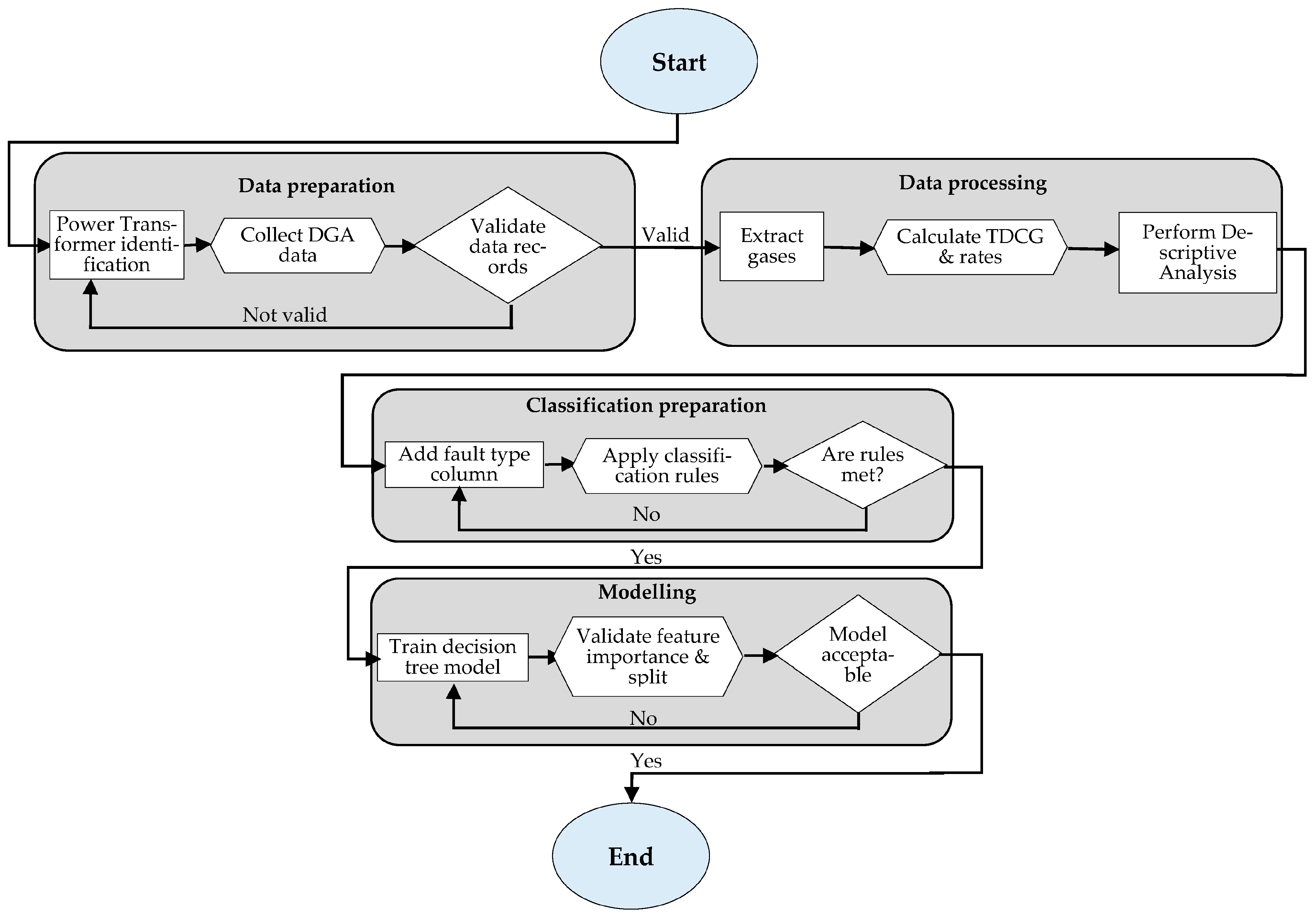
Figure 1 shows the schematic diagram detailing the process utilised in this study to build the proposed SGDT framework, which integrates advanced statistical analysis with decision tree learning using DGA data from a single power transformer. Using one transformer made it possible to closely study how faults develop and how gas behaves under steady working conditions, reducing differences caused by transformer design, load, maintenance, and environment. The results show that the method works well on a real monitored transformer. However, testing with data from many transformers is valuable to consider in the future.

The dataset was collected directly from an online DGA monitoring system over five years and kept in its original form to keep the real-world measurement details. Small negative values showed up in a few gas measurements, mainly for acetylene (C₂H₂), with rare cases in H₂, CH₄, CO, and CO₂. These values come from measurement uncertainty, sensor baseline shifts, calibration changes, and limits in analysis when gas levels are close to the detection limit. Although these values are not physically negative gas amounts, they are actual readings from the monitoring equipment during operation. So, the values were kept to ensure the fault classification model was built and tested using realistic field data that reflects real use conditions.

The work began with identifying the transformer and collecting its dissolved gas records. Following this was data validation; the relevant gases were extracted, and TDCG values and generation rates were calculated. Descriptive statistical analysis was then performed to understand gas behaviour patterns and establish data-driven thresholds for transformer fault identification. Based on these statistical findings, fault classification rules were developed and used to assign fault labels to the dataset. The labelled dataset was then used to train and test the decision tree model. Traditional DGA diagnostic methods, like the Duval Triangle, provided background and comparison points.

3.1. Selection of Statistical Estimation Methods

To make sure the description of the DGA dataset is accurate, several ways to estimate average values and spread were tested.

Table 1. Preferred methods for estimating confidence intervals of statistical measures.

Confidence Intervals	Methods Considered	Preferred Method	Justification for Preference
Mean	T-Model, Normal Model, Bootstrap	Bootstrap	It provides confidence intervals that do not depend on the normal distribution, which works well for DGA datasets.
Standard Deviation	Analytical (Chi-squared), Bootstrap	Bootstrap	Works better with uneven data and strange values; shows true differences in gas measurements more clearly.
Variance	Analytical (Chi-squared), Bootstrap	Bootstrap	Includes a wider, more accurate range of differences; stops underestimating uncertainty in data that often contains mistakes.

shows the methods looked at for each statistic, highlights the chosen method, and explains why based on features of the data like unusual values and uneven distributions. The bootstrap method was selected as the preferred approach in all cases due to its robustness and independence from parametric assumptions.

3.2. Classification Rule Application

This study created guidelines to identify transformer problems by looking at gas data from transformer samples. These rules set clear limits to identify specific fault types using summary statistics and gas patterns found in the data. Summary statistics were calculated for all variables, including main combustible gases and other gases like CO₂, O₂, H₂O, TDCG, and generation rates. Threshold values were set for each variable to describe their statistical patterns. However, only six gases (H₂, CH₄, C₂H₂, C₂H₄, C₂H₆, and CO) were selected to establish fault classification rules.

Table 2. Statistically derived gas thresholds for transformer fault identification.

Rule	Fault Type	Conditions	Descriptive Statistics Justification
1	D2—High Discharge	C2H2 > 1.0, H2 > 200, CO > 90	C2H2 95th = 0.41 → >1.0 is extreme; H2 median = 336.8 → >200 is frequent; CO 95th = 84 → >90 is elevated
2	D1—Low Discharge	C2H2 > 0.5, CH4 > 70, H2 > 150	C2H2 above IQR; CH4 mean = 77.8 → >70 valid; H2 >150 is conservative but below the median
3	PD—Partial Discharge	H2 > 300, CH4 < 80, C2H2 < 0.2	H2 >300 aligns with discharge zone; CH4 < mean; C2H2 < 0.2 fits 75th percentile
4	T3—High Thermal	C2H4 > 26.8, C2H6 > 300, CO > 90	C2H4 max = 26.8 → capped; C2H6 95th = 299.6; CO > 90 exceeds 95th percentile
5	T2—Medium Thermal	C2H4 20–26.8, C2H6 280–300, CO 70–84	All within IQR–95th window; elevated but not extreme
6	T1—Low Thermal	C2H4 < 20, C2H6 < 280, C2H2 < 0.2	All values below 75th percentile; typical of mild thermal faults
7	Mixed Fault	≥2 of: C2H2 > 1.0, H2 > 200, CO > 90, CH4 > 70, C2H4 > 26.8, C2H6 > 300	Based on high correlations: CH4–C2H6 = 0.94, CO–C2H6 = 0.90; overlaps in fault indicators
8	Normal	All gases below all thresholds	Based on median and IQR, healthy gas levels with no abnormal signatures

describes each transformer fault type based on specific gas concentration thresholds. These thresholds were chosen using descriptive statistics such as the median, Interquartile Range (IQR), 75th percentile, 95th percentile, and maximum, depending on how each gas behaves in the dataset.

For example, C₂H₂ levels are usually very low, so values above the 95th percentile are seen as abnormal. H₂ is found more often, so using limits based on the middle value or spread is better. Gases linked to heat damage, like C₂H₄ and C₂H₆, usually rise slowly, so limits set between the middle spread and the 95th percentile help show how serious the fault is. CO, often linked to insulation ageing, is checked using values between the 75th and 95th percentiles. These limits were chosen based on how each gas is spread out and its known connection to certain fault types, helping to make reliable rule-based decisions. Fault rules were made only for the six main gases to keep the diagnosis relevant. In contrast, when training the ML model, all available variables, including those excluded from rule development, were incorporated as features to enable the model to identify additional patterns and enhance fault prediction robustness.

Although eight fault categories were defined through the statistical rule-development process, only six fault classes (D1, PD, T1, T2, Mixed, and Normal) were represented in the classified dataset. The D2 (High Discharge) and T3 (High Thermal) categories were defined based on extreme threshold combinations from the upper tails of gas concentration distributions. Since no observations in the operational dataset met these criteria, only the six represented fault classes were included in the decision tree modelling and performance evaluation.

Rule 1 flags a high discharge fault when C₂H₂ goes above 1.0 ppm, H₂ is over 200 ppm, and CO is higher than 90 ppm. These values are well beyond what is usually seen and point to strong arcing inside the transformer. Rule 2 suggests a low discharge if C₂H₂ is above 0.5 ppm, CH₄ is over 70 ppm, and H₂ is more than 150 ppm. This combination indicates a less intense but still abnormal discharge. In Rule 3, partial discharge is likely when H₂ is greater than 300 ppm while both CH₄ and C₂H₂ stay low, which is a typical pattern for ionisation or corona activity.

Rule 4 indicates high thermal stress when C₂H₄ and C₂H₆ both exceed their usual limits, and CO also rises, all pointing to overheating. Rule 5 describes a medium thermal fault if C₂H₄, C₂H₆, and CO fall between common and extreme values, meaning there is heating but not at critical levels. Rule 6 is used when C₂H₄, C₂H₆, and C₂H₂ remain low, which matches what is expected from minor heating. Rule 7 covers cases where two or more gases from the group C₂H₂, H₂, CO, CH₄, C₂H₄, and C₂H₆ are elevated at the same time, showing signs of both thermal and electrical faults happening together. Rule 8 is used when all gas levels are normal, showing that the transformer is working without any problems or damage. Stray gassing was not listed as a separate category in the dataset, so it was not studied. Future work will add labelled stray-gassing cases to see whether the SGDT system can distinguish stray gassing from actual transformer faults.

3.3. Decision Tree Model Configuration

The decision tree model was created to check if the gas concentration rules for fault labelling matched real data patterns. The goal was not to diagnose transformer faults on its own but to see if the fault classification rules based on statistics could be reliably learned and applied to new data. A dataset of 33,778 records was split into training (64%), validation (16%), and test (20%) parts. The model was set with a maximum depth of 4, needed at least 20 records to make a split, and required at least 15 records in each end node. Feature scaling and a fixed random seed were used to keep results consistent. A complexity penalty of 0.1 was added to reduce overfitting. The full model reached 98% accuracy on the test data with 119 splits. A simpler decision tree with a maximum depth of 3 was also made to help with visualisation. This simpler model made it easier to understand while keeping important splits based on gases like C₂H₂, H₂, CH₄, and C₂H₄, matching the original rule-based system.

Table 3. Decision Tree model performance across multiple random seed iterations.

Iteration	Random Seed	Accuracy	Precision	Recall	F1-Score	Area Under Curve (AUC)
1	1	0.993	0.981	0.980	0.980	0.987
2	10	0.994	0.982	0.981	0.981	0.984
3	20	0.994	0.984	0.983	0.983	0.988
4	30	0.993	0.982	0.980	0.981	0.988
5	40	0.993	0.979	0.978	0.979	0.983
6	50	0.994	0.984	0.983	0.983	0.985
7	60	0.994	0.984	0.983	0.983	0.988
8	70	0.994	0.984	0.983	0.983	0.989
9	80	0.993	0.980	0.979	0.979	0.988
10	90	0.993	0.980	0.980	0.980	0.985
Mean		0.9935	0.9820	0.9810	0.9812	0.9865
Standard Deviation		0.0005	0.0019	0.0019	0.0017	0.0021

presents decision tree model performance across multiple random-seed iterations. To assess the robustness of the proposed Decision Tree model against variations in data partitioning, the model was evaluated over ten iterations using different random seeds. The average Accuracy, Precision, Recall, F1-score, and AUC were 0.9935 ± 0.0005, 0.9820 ± 0.0019, 0.9810 ± 0.0019, 0.9812 ± 0.0017, and 0.9865 ± 0.0021, respectively. The low standard deviations indicate that the model exhibits stable performance and good generalisation capability across different dataset partitions.

4. Results

4.1. Case Study Overview

The transformer under study is a commissioned three-winding unit rated at 275 kV (primary), 88 kV (secondary), and 22 kV (tertiary), with corresponding power ratings of 160 MVA for the primary and secondary windings, and 315 kVA for the tertiary, and is equipped with an on-load tap changer (OLTC). The transformer has a YNyn0d1 vector group setup, giving easy access to neutral points on both the primary and secondary windings. It works with a standard impedance level and does not have extra cooling. These electrical and setup features are important for the proposed hybrid fault classification method because they directly influence fault behaviour, gas formation patterns, and diagnostic accuracy. The dataset used in the study consisted of 33,778 hourly records collected over a five-year period.

4.2. Statistical Analysis of DGA Data

4.2.1. Analysis of Key Diagnostic Gases

Table 4. Central tendency statistics for diagnostic gases used in transformer fault classification.

Gas	Median (ppm)	Mean (ppm)	Total	Comments
H2	336.8	312.664	1.056 × 10+7	>200 ppm indicates active discharge; consistent with “Caution–Danger” (Table 2) and Rule 1 (D2).
CH4	79.6	77.8	2.628 × 10+6	>70 ppm signals low discharge; within “Caution” zone (Table 2); aligns with Rule 2 (D1).
C2H2	0.1	0.115	3897.5	>0.5–1.0 ppm shows arcing; exceeds normal range (Table 2); supports Rules 1–2.
C2H4	11.6	12.791	432,065.71	>20 ppm marks thermal fault onset; matches “Caution–Danger” range (Table 2); Rules 4–6.
C2H6	273.2	266.115	8.989 × 10+6	>280 ppm reflects high thermal stress; beyond “Danger” limit (Table 2); Rules 4–5.
CO	79.2	77.457	2.616 × 10+6	>90 ppm indicates insulation aging; relates to “Abnormal” range (Table 2); Rules 1, 4–5.
TDCG	769.225	746.943	2.523 × 10+7	>720 ppm shows gas accumulation; in “Caution–Abnormal” zone (Table 2); supports Rule 7.

gives a snapshot of typical dissolved gas levels found in transformer oil by summarising the median, mean, and total concentration of each gas. These values are important because they base the fault classification rules on real measurements. For example, the average H₂ concentration is 336.8 ppm, which supports picking 200 ppm and 300 ppm as limits in Rules 1 and 3. These limits are much lower than the average and help detect unusual increases. The average CH₄ level is 79.6 ppm, showing that the 70 ppm limit in Rule 2 works well as an early alert.

C₂H₂ shows a typical value of 0.1 ppm, which explains why thresholds like 0.5 and 1.0 ppm are flagged; levels above this range are rare and suggest fault activity. The middle levels of C₂H₄ and C₂H₆, measured at 11.6 and 273.2 ppm, help explain thermal fault limits that range from 20 to 300 ppm. The middle CO level of 79.2 ppm supports using limits between 70 and 90 ppm. The middle amount of TDCG, at 769.225 ppm, shows its importance as a sign of overall gas amount. While these average values set usual ranges, they do not by themselves cover extreme cases or unusual patterns. Therefore, further statistical analysis is needed to support robust fault detection.

4.2.2. Dispersion Metrics of Key Diagnostic Gases

Table 5. Dispersion statistics for diagnostic gases in transformer DGA records.

Gas	Std. Deviation	CV	IQR	Variance	Range	Minimum	Maximum
H2	115.02	0.368	171.7	13,229.652	500.4	−1.5	498.9
CH4	12.496	0.161	3.4	156.151	101.9	−5.8	96.1
C2H2	0.171	1.484	0.21	0.029	4.1	−2.9	1.2
C2H4	4.5	0.352	1.2	20.254	26.8	0	26.8
C2H6	45.838	0.172	30.8	2101.11	353.9	0	353.9
CO	12.643	0.163	4	159.854	97.25	−0.45	96.8
TDCG	158.618	0.212	199.645	25,159.8	966.56	0	966.56

shows how much each gas varies by listing the standard deviation, the coefficient of variation (CV), and the IQR. These measures help show how gas levels vary around normal values. This information was especially useful when setting data-based limits in the hybrid fault classification method, where ranges based on percentiles needed to match the real differences seen in the data.

For C₂H₂, a high CV of 1.484 and an IQR of 0.21 validate the use of sharp thresholds like 0.5 and 1.0 since such levels fall well outside typical fluctuation. H₂ shows a standard deviation of 115.02 and an IQR of 171.7, supporting 200 and 300 as suitable values to detect deviation from normality. CH₄, with low variation (standard deviation 12.5), justifies a conservative threshold of 70, which stands out from its usual spread. The wide range of C₂H₆, measured at 353.9, along with its middle spread (IQR) of 30.8, supports its use in Rules 4 and 5, which use cut-off values of 280 and 300 to distinguish between moderate and high heat conditions.

4.2.3. Confidence Interval Estimates for Transformer DGA Data

Table 6. Confidence intervals (95%) for mean, standard deviation, and variance of key gases.

Key Dissolved Gases	95% Confidence Interval Mean		95% Confidence Interval Std. Dev.		95% Confidence Interval Variance
	Upper	Lower	Upper	Lower	Upper	Lower
H2	313.849	311.428	115.826	114.213	13,415.73	13,044.637
CH4	77.925	77.665	12.904	12.124	166.508	146.999
C2H2	0.117	0.113	0.174	0.169	0.03	0.029
C2H4	12.836	12.746	4.549	4.449	20.698	19.793
C2H6	266.574	265.611	47.102	44.599	2218.6	1989.028
CO	77.585	77.318	13.04	12.267	170.048	150.484
TDCG	748.628	745.317	161.551	155.902	26,098.773	24,305.58

shows the 95% confidence ranges for the average, spread, and variation of each gas, which helps to see how consistent the gas behaviour is when picking thresholds. These ranges confirm that important gas measurements used in the hybrid rules are stable. For example, H₂ has a small confidence range for the average (311.4 to 313.8), and its spread is between 114.2 and 115.8, which supports using 200 and 300 as fault thresholds for discharge.

For CH₄, the average ranges from 77.7 to 77.9, with a variation between 12.1 and 12.9, confirming the 70 ppm Rule 2 limit as a clear increase. The upper limits of the average confidence ranges for C₂H₄ and C₂H₆ are 12.84 ppm and 266.57 ppm, respectively, supporting the use of higher cut-off points like 20, 280, and 300 ppm in the classification rules. These limits are set beyond the normal range and help spot unusual heat activity. Although these ranges use statistics to choose the cutoffs, they might not catch all unusual or extreme values. In these cases, looking at data percentiles and how data is uneven helps better identify outliers and uneven data patterns.

4.2.4. Quantile and Percentile Distribution of DGA Data

Table 7. IQRs, quintiles, and percentile extremes of key dissolved gases.

Key Dissolved Gases	Interquartile Statistics			Percentile Extremes
	25th Percentile	50th Percentile	75th Percentile	5th Percentile	95th Percentile
H2	231.8	336.8	403.5	102.5	444.1
CH4	78	79.6	81.4	75.8	83.1
C2H2	0	0.1	0.21	−0.14	0.41
C2H4	11.1	11.6	12.3	10.3	23.6
C2H6	257	273.2	287.8	240.4	299.6
CO	77.1	79.2	81.1	74.2	84
TDCG	659.015	769.225	858.66	572.364	897.94

shows data summaries based on parts of the data, including ranges and extreme values, giving a clear picture of how data is spread across segments. These summaries helped select the best fault-detection limits in the hybrid method. The 95th percentile of H₂ is 444.1, and the 75th percentile is 403.5, showing that the thresholds for Rules 1 and 3, set at 200 and 300, are in the higher part of the data and help detect early and important increases.

CH₄ has a narrow band between the 75th and 95th percentiles (81.4 to 83.1), and the Rule 2 threshold of 70 falls below it, ensuring it flags deviations from routine levels. C₂H₂ has a 95th percentile value of 0.41, which supports the importance of Rule 1 and Rule 2 limits at 1.0 and 0.5. For C₂H₄ and C₂H₆, 95th percentile values of 23.6 and 299.6 support using 20 and 300 as limits for medium and high heat conditions. These percentile-based results improve how well the rules detect both slow changes and rare spikes.

4.2.5. Distribution Characteristics of Key Dissolved Gases

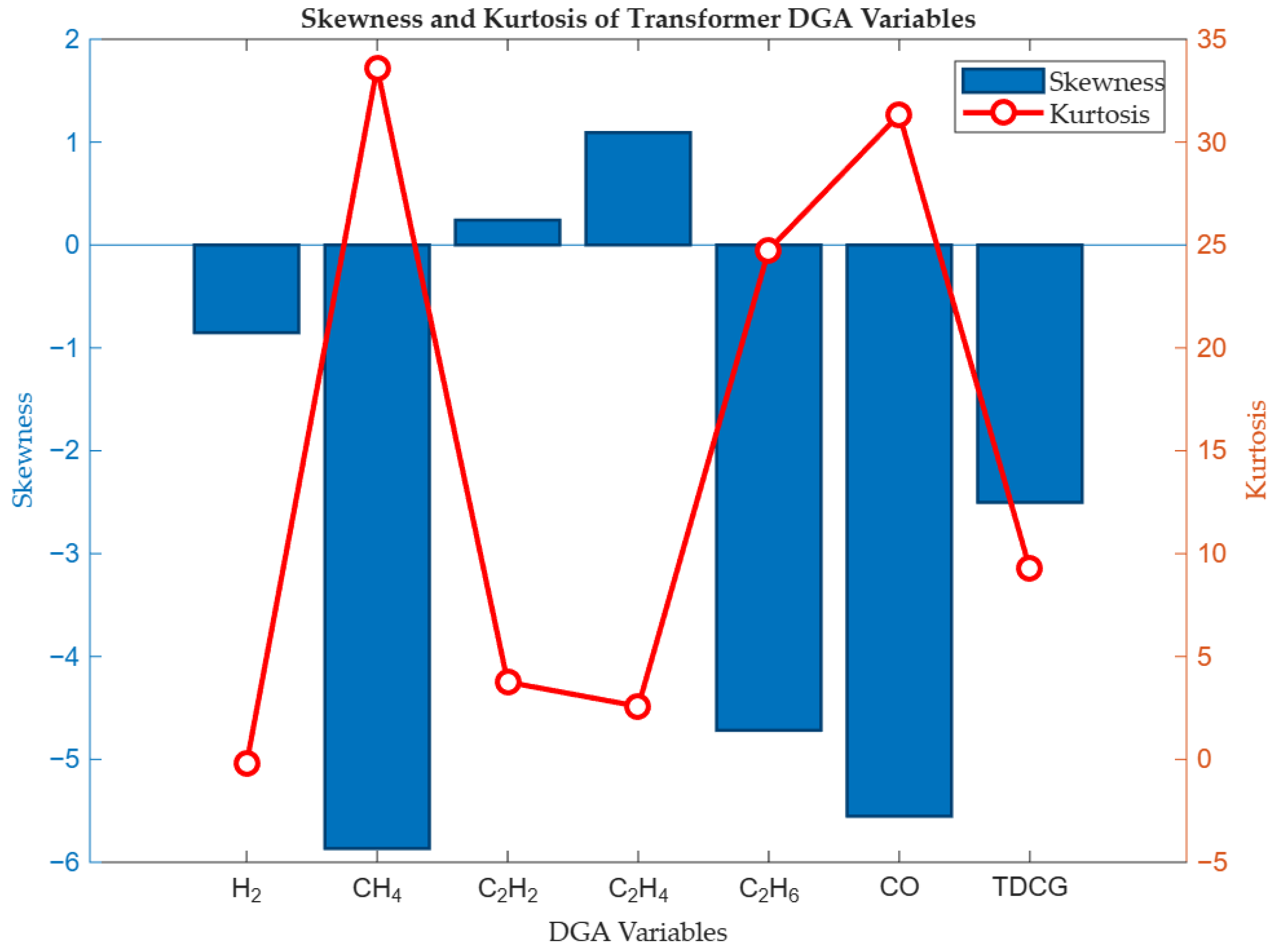
Figure 2 shows a visual comparison of the shape and spread of the transformer DGA variables. The figure highlights how the gas distribution makes it easier to spot variables with different degrees of variance and extreme values. So, the differences indicate that the DGA variables do not follow a consistent pattern, supporting the use of gas-specific limits and diagnostic rules for more accurate transformer fault detection.

Table 8. Skewness and kurtosis of power transformer DGA variables.

Key Dissolved Gases	Skewness	Kurtosis
H2	−0.853	−0.214
CH4	−5.866	33.604
C2H2	0.242	3.757
C2H4	1.092	2.575
C2H6	−4.718	24.764
CO	−5.552	31.34
TDCG	−2.503	9.261

shows the skewness and kurtosis values for each gas, giving information about how the data is spread out and the chance of extreme values. These factors are important when setting fault-classification limits based on statistics. Variables with high skewness and kurtosis show unusual patterns and a higher chance of fault-related unusual values. These statistical measures helped select and explain the gas concentration limits in the proposed rule-based classification system, making fault detection more dependable. CH₄ and CO have strong left skewness (–5.866 and –5.552) and very high kurtosis values over 30, which indicate heavy tails and a higher chance of unusual values. This confirms the need to use conservative thresholds, such as 70 and 90 in Rules 2 and 4, to avoid false positives.

C₂H₆ and TDCG also show left skewness and high kurtosis, supporting the upper threshold selections of 280 and 300 to capture critical cases without being misled by long-tailed noise. C₂H₄, which shows a small lean to the right (1.092), supports using uneven limits between Rules 4 and 6. C₂H₂, with a nearly balanced spread and moderate sharpness, confirms it as a rare but important fault gas, where clear spikes instead of slow rises show discharge activity. While these shape measures help adjust classification, they should be used together with spread and range analysis to avoid mistaking normal changes for fault start.

4.2.6. Association Matrix

Covariance Analysis of Dissolved Gases

Table 9. Covariance matrix for key DGA variables in the power transformer.

Key Dissolved Gases	H2	CH4	C2H2	C2H4	C2H6	CO	TDCG
H2	13,229.652	748	−2.802	−180.929	2418.318	378.298	16,590.537
CH4	748	156.151	0.135	23.1	536.499	150.047	1613.932
C2H2	−2.802	0.135	0.029	0.034	−0.099	0.3	−2.402
C2H4	−180.929	23.1	0.034	20.254	121.082	32.293	15.834
C2H6	2418.318	536.499	−0.099	121.082	2101.11	522.098	5699.008
CO	378.298	150.047	0.3	32.293	522.098	159.854	1242.89
TDCG	16,590.537	1613.932	−2.402	15.834	5699.008	1242.89	25,159.8

shows how gas concentrations change together across the dataset, revealing which gases tend to rise or fall at the same time. The strong positive link between C₂H₆ and H₂ (2418.318), and between C₂H₆ and CH₄ (536.499), means these gases increase together during thermal or low-energy discharge conditions. This matches their combined presence in Rules 2, 4, and 5. The covariance of H₂ and TDCG (16,590.537) further supports using H₂ as a leading indicator for overall fault gas accumulation.

Negative covariance between H₂ and C₂H₄ (–180.929) suggests an inverse relationship, possibly distinguishing electrical from thermal fault behaviour, and justifying the separation of H₂ and C₂H₄ in Rules 3 and 4. C₂H₂ shows low or negative relationships with most gases, including a small negative value with TDCG (–2.402), which supports using it as a specific discharge indicator rather than a general fault marker. These relationship patterns helped improve the rule conditions by showing which gases give overlapping or separate diagnostic information. However, because these relationships are not standardised and depend on scale, they should be considered together with correlation to correctly judge how strong the connections are.

Correlation Analysis of Dissolved Gases

Table 10. Pearson correlation matrix for key DGA variables in the power transformer.

Key Dissolved Gases	H2	CH4	C2H2	C2H4	C2H6	CO	TDCG
H2	1	0.52	−0.142	−0.35	0.459	0.26	0.909
CH4	0.52	1	0.063	0.411	0.937	0.95	0.814
C2H2	−0.142	0.063	1	0.045	−0.013	0.139	−0.088
C2H4	−0.35	0.411	0.045	1	0.587	0.568	0.022
C2H6	0.459	0.937	−0.013	0.587	1	0.901	0.784
CO	0.26	0.95	0.139	0.568	0.901	1	0.62
TDCG	0.909	0.814	−0.088	0.022	0.784	0.62	1

shows the Pearson correlation values between dissolved gases, helping to explain how closely the levels of different gases are linked. These relationships indicate which gases tend to increase or decrease together, suggesting they may come from the same underlying fault. CH₄ and C₂H₆ show a very high positive correlation of 0.937, reinforcing their joint use in Rules 2, 4, and 5, where both gases reflect thermal or low-energy discharge progression. CO is also strongly correlated with CH₄ (0.95) and C₂H₆ (0.901), which supports its threshold-based role in Rules 4 and 5 for detecting thermal stress or insulation degradation.

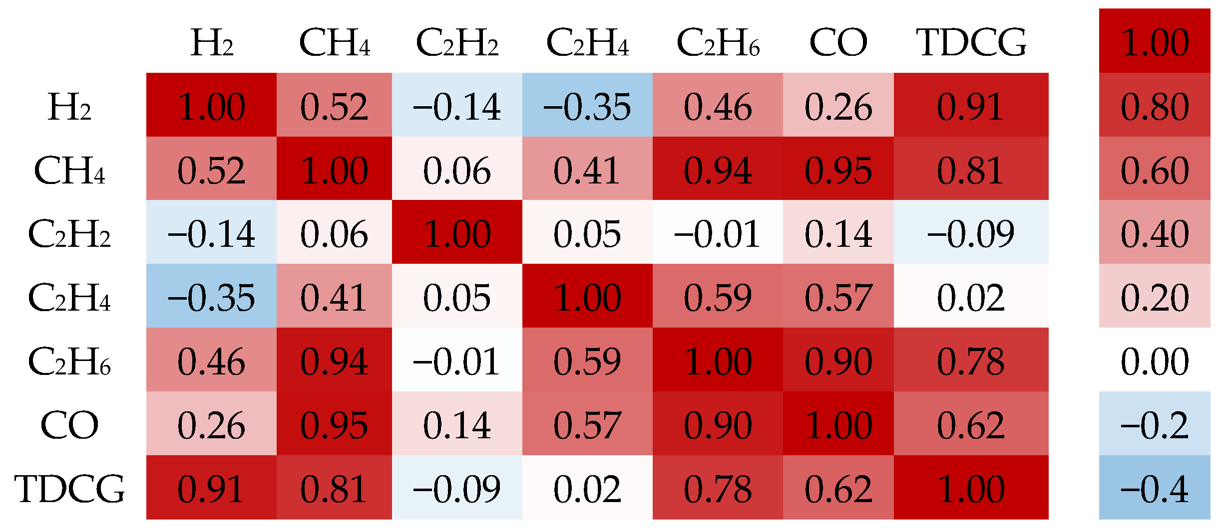
H₂ and TDCG show a strong correlation of 0.909, confirming H₂ contribution to total gas build-up and supporting its prominence in multiple rules, including mixed fault classification. Conversely, C₂H₂ has weak or negative correlations with most gases, including –0.142 with H₂ and –0.088 with TDCG, validating its role in isolating high-energy or partial discharges (Rules 1 and 3) where other gases remain low. Figure 3 shows how the different gases change in relation to one another. CH₄, C₂H₆, and CO move together and tend to increase when the oil is exposed to heat, while C₂H₂ stays separate, which matches its link to arcing. The figure gives a straightforward picture of these patterns and supports what is presented in

Table 11. Normalised confusion matrix for transformer fault type classification.

		Observed
		D1	Mixed	Normal	PD	T1	T2
Predicted	D1	0.02	0	0	0	0	0
	Mixed	0	0.43	0	0	0	0
	Normal	0	0	0.05	0	0	0
	PD	0	0	0	0.16	0	0
	T1	0	0	0	0	0.26	0
	T2	0	0.01	0	0	0	0.06

.

These correlations confirm that the gas combinations used in the classification rules were not arbitrarily selected but based on clear co-behaviour patterns in the dataset. Correlation only shows straight-line relationships. If gases are linked in more complex ways, this method might not capture them. To fill these gaps, future research should look into other methods that do not rely on simple straight-line patterns.

4.3. Decision Tree Model Analysis

While the rule-based fault type allocation focused only on combustible gases like H₂, CH₄, C₂H₂, C₂H₄, C₂H₆, and CO, the decision tree model was trained using a larger and more detailed set of input data to identify complex fault patterns. This classification method was chosen because it is easy to understand and can handle complex relationships. The dataset had 33,778 dissolved gas records, which were split into training (64%), validation (16%), and test (20%) groups. Input variables included both combustible gases and other indicators, such as CO₂, O₂, H₂O, TDCG, and TDCG generation rates measured in parts per million per hour and per day. These variables were added to provide additional context and help the model capture patterns that may not be directly used in the fault classification rules.

4.3.1. Confusion Matrix Evaluation of Fault Classification Model

Table 11 presents the normalised confusion matrix for the classification model, showing the proportion of correctly and incorrectly predicted fault types. It evaluates how well the decision tree replicated the rule-based classification labels developed in the hybrid method. In a normalised matrix, each cell value goes from 0 to 1. Values close to 1 show a stronger match between predicted and actual fault labels, while a value of 0 means the model did not make any correct predictions for that class. The diagonal values show correct classifications, and the off-diagonal values show wrong classifications. The model is best at identifying the Mixed class, with a correct prediction rate of 0.43. This is followed by T1 at 0.26 and PD at 0.16, showing that the model is better at recognising overlapping fault patterns and thermal issues.

In contrast, the model is less accurate for Normal and D1 cases, with scores of 0.05 and 0.02. This means it is hard to distinguish healthy conditions or low-energy discharges from other fault types, especially when gas patterns look alike. The confusion matrix shows that the model’s classification accuracy varies between groups, which supports using both fixed limits and ML methods to handle unclear cases. However, the table does not show total counts, which are needed to understand class imbalance and evaluate error costs.

4.3.2. Class Distribution Analysis Across Data Partitions

Table 12. Proportions of fault type classes in the whole dataset, training, validation, and test sets.

Fault Types	Data Set	Training Set	Deviation (Training)	Validation Set	Deviation (Validation)	Test Set	Deviation (Test)
D1	0.019	0.02	5.26%	0.02	5.26%	0.019	0.00%
Mixed	0.442	0.443	0.23%	0.446	0.90%	0.438	0.90%
Normal	0.056	0.055	1.79%	0.053	5.36%	0.06	7.14%
PD	0.161	0.162	0.62%	0.156	3.73%	0.159	1.24%
T1	0.253	0.251	0.79%	0.253	0.00%	0.261	3.16%
T2	0.069	0.069	0.00%	0.073	5.80%	0.064	7.25%

shows how each fault type is spread across the whole dataset, including the training, validation, and test parts. This table checks if the dataset sections used for training kept the original class balance needed for fair model testing. Mixed faults are the most common at around 44 per cent, while D1 faults make up only 2 per cent. The lower recall and prediction rates for the D1 and Normal classes can be traced back to the imbalance in class distribution. These classes have fewer examples, making them more challenging for the model to learn.

The percentage deviation between each subset and the overall dataset was included to assess partitioning consistency. Deviations below 5% show that the data was divided with a balanced mix of classes in the training, validation, and test sets. Also, having similar class proportions in these sets supports the trustworthiness of the results. This balance shows that the model was tested fairly and suggests that it will work well with new data.

4.3.3. Classification Performance Evaluation

Table 13. Model performance metrics per fault class.

Performance Metrics	D1	Mixed	Normal	PD	T1	T2	Average/Total	Comments
Support	126	2956	403	1077	1763	430	6755	Mixed and T1 dominate the dataset.
Accuracy	0.996	0.985	0.991	1	0.998	0.99	0.993	Accuracy > 0.98 shows stable overall performance.
Precision (Positive Predictive Value)	0.925	0.992	0.929	1	0.994	0.874	0.981	Few false positives; PD and T1 are perfect.
Recall (True Positive Rate)	0.881	0.974	0.911	1	1	0.988	0.98	D1 and Normal slightly lower due to limited samples.
False Positive Rate	0.001	0.006	0.004	0	0.002	0.01	0.004	Very low misclassification risk.
False Discovery Rate	0.075	0.008	0.071	0	0.006	0.126	0.048	Higher for T2 due to class overlap.
F1 Score	0.902	0.983	0.92	1	0.997	0.928	0.98	All > 0.9; excellent precision–recall balance.
Area Under Curve (AUC)	1	0.994	0.932	1	0.999	1	0.987	Near 1.0 indicates strong class separation.
Negative Predictive Value	0.998	0.98	0.994	1	1	0.999	0.995	Reliable negative predictions.
True Negative Rate	0.999	0.994	0.996	1	0.998	0.99	0.996	Very low false alarm probability.
False Negative Rate	0.119	0.026	0.089	0	0	0.012	0.041	D1 most missed; PD perfect recall.
False Omission Rate	0.002	0.02	0.006	0	0	7.976 × 10−4	0.005	Negligible false negatives.

shows how well the model performs for different fault types, measured by accuracy, precision, recall, F1 score, and area under the curve (AUC). These results help confirm whether the model is correctly picking up the fault patterns defined by the hybrid rules. By checking each metric, it is possible to see where the model is working well and where it may need improvement. The model achieved an overall accuracy of 0.993 and an average F1 score of 0.98, indicating excellent general alignment with the rule-based structure. PD and T1 get recall and F1 scores of 1 and 0.997, showing that the decision tree correctly recognises thermal and partial discharge patterns.

The model picks up D1 well, with a recall of 0.881 and a precision of 0.925, even though there were fewer examples to learn from. T2, on the other hand, has a higher false discovery rate of 0.126. This may be because its gas levels are close to those of T1, making it harder for the model to separate them. The AUC scores for most classes are close to 1, showing that the model works well and reliably across different fault types. Even though the classes are not evenly spread out, the model keeps high accuracy and correctly identifies non-fault cases across all fault groups. The low average false positive rate of 0.004 and false omission rate of 0.005 mean there is little chance of false alarms or missed faults. These results show that the classifier works well for both common and rare fault types, making it suitable for real-world transformer condition checks.

4.3.4. Feature Importance Evaluation

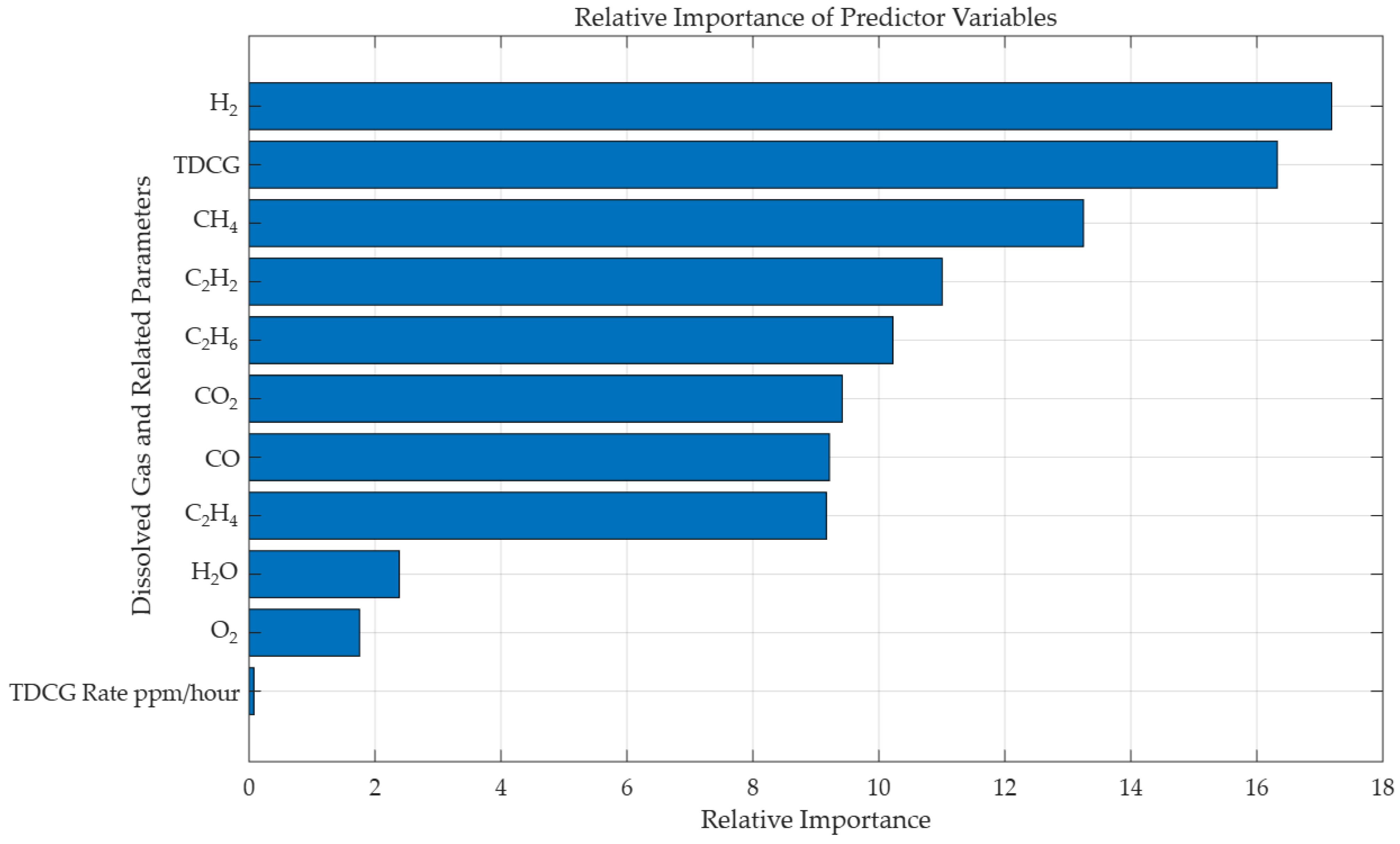
Figure 4 shows the importance of each feature in identifying transformer faults. It points out that the model primarily relies on a few key gas indicators, while other variables have less effect on classification performance.

Table 14. Feature importance metrics in transformer fault classification.

Dissolved Gas and Related Parameters	Relative Importance	Mean Dropout Loss
H2	17.187	1757.609
TDCG	16.324	186.38
CH4	13.248	2027.873
C2H2	11.004	2509.57
C2H6	10.222	2757.883
CO2	9.417	72.498
CO	9.215	191.101
C2H4	9.166	765.372
H2O	2.385	72.498
O2	1.755	72.498
TDCG Rate (ppm/hour)	0.077	72.498

shows that H₂, TDCG, and CH₄ have the greatest effect on how the model detects faults. Their scores are 17.2 for H₂, 16.3 for TDCG, and 13.2 for CH₄, reflecting how often the model uses these gases to make decisions. This is consistent with their role in Rules 1 to 3 and confirms that they are key to the way the model operates. C₂H₂ also has a substantial impact, scoring 11.0, which supports its role in recognising high-energy discharge events.

When looking at dropout loss, C₂H₆ and C₂H₂ have the highest values at 2757.88 and 2509.57. The drop in model accuracy when these gases are left out shows how important they are for keeping prediction quality high. On the other hand, CO₂, H₂O, and O₂ have the smallest dropout loss of 72.498, meaning they have little effect on telling faults apart and offer limited help for diagnosis here. The TDCG rate is also the lowest and, because it hardly affects classification results, can be left out of future model inputs. These results support the hybrid model by showing that gases found important by rule-based methods are also the main ones chosen by ML.

4.3.5. Decision Tree Splitting Characteristics

Table 15. Main variable splits and the related improvement in error at each tree level.

Dissolved Gas and Related Parameters	Obs. in Split	Split Point	Improvement
C2H6	21,618	0.302	2176.99
CH4	8377	0.172	1890.428
TDCG	5789	−0.822	104.959
CO	120	0.897	26.284
C2H4	2588	0.824	555.388
C2H2	607	0.465	190.456
CO	1981	0.521	407.932
C2H2	13,241	0.465	3478.716
H2	4757	−0.979	1175.791
C2H2	3835	2.275	433.931
C2H2	922	2.275	214.455
CH4	8484	0.172	1106.05
H2	5631	−0.11	2769.49

shows the most important variable splits at each level of the decision tree, based on how much they improve the model. C₂H₆ appears often, with a split point of 0.302 leading to a big improvement of 2176.99, confirming its key role in detecting thermal faults. CH₄, with a split at 0.172 improving deviance by 1890.428, and H₂, with a split at –0.11 yielding an improvement of 2769.49, show strong separation power, supporting their placement in Rules 2 and 3.

C₂H₂, appearing three times with consistent split points around 0.465 and 2.275, reinforces its importance in discharge classification. The presence of TDCG and CO at different levels, along with moderate improvements, shows they play a smaller role in improving class boundaries. These split points match the statistical limits set earlier in the study, confirming the agreement between rule-based and machine-learned patterns.

4.3.6. Receiver Operating Characteristic (ROC) Curve for Multi-Class Fault Classification

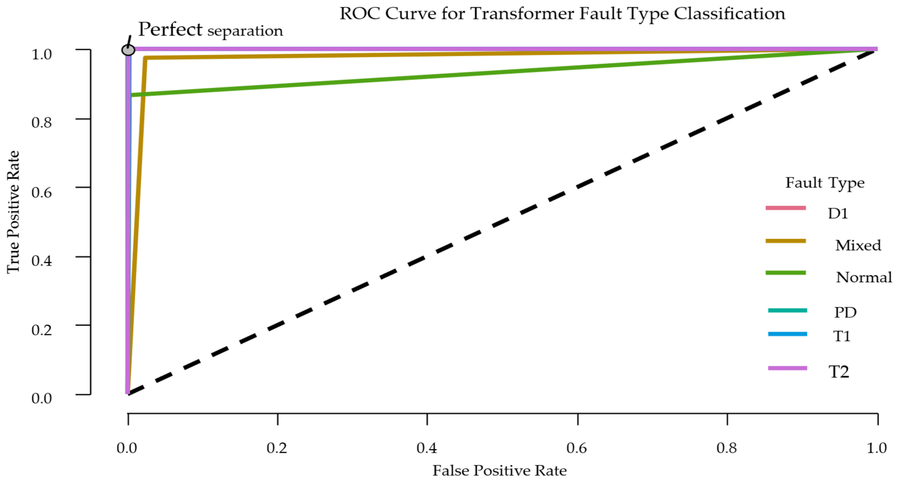
Figure 5 displays the ROC curves for all six fault types, comparing the actual positive rate to the false positive rate. This method checks how well the model can distinguish different classes at various cutoff points and supports the hybrid method by testing how trustworthy the rule-based labels are through prediction. The curves for PD, T1, T2, and D1 are near the top-left corner, with area under the curve (AUC) values close to 1.0, showing that the model correctly identifies these faults. In contrast, the curve for the Normal class is flatter, which points to some overlap with other classes and matches its lower precision and recall. Overall, the ROC curves confirm that the model is learning the same gas separation patterns defined in the rule set. Still, because ROC curves do not show class imbalances or the types of errors made, they should be used alongside the confusion matrix to get a complete picture of model performance.

At low false positive rates, the close grouping of the D1, PD, T1, T2, and Mixed receiver operating characteristic (ROC) curves near the top-left area shows that the model needs only small increases in false alarms to reach almost the best detection performance. This feature is especially useful for checking transformer conditions, where false fault warnings can lead to unnecessary maintenance and inspections. The results show that the proposed hybrid classification system finds a good balance between detecting faults correctly and making dependable decisions in real-world utility situations.

4.3.7. Effect of Complexity Penalty on Classification Accuracy

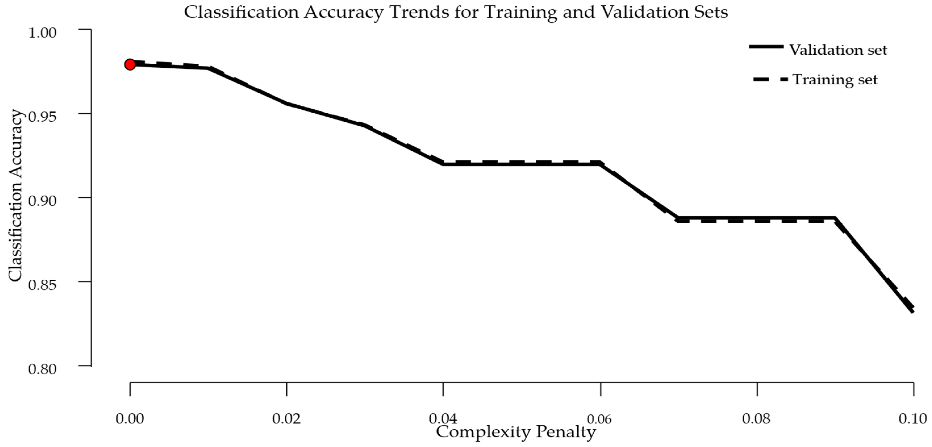
Figure 6 shows how classification accuracy changes as the complexity penalty increases. This looks at the balance between keeping the model simple and making it work well, which is important for making rule-based systems easy to understand while still accurate. The best accuracy happens at a low penalty, near 0.00, showing that the chosen decision tree depth works almost perfectly. When the penalty increases, accuracy drops, meaning the model is too simple. These results suggest using a fairly shallow tree to keep the structure clear without losing accuracy. The close match between the training and validation curves shows the model works well on both datasets. This match supports the choice of gas split points in the hybrid framework. Overall, the figure shows that the selected tree structure is both accurate and can be applied generally.

4.3.8. Decision Tree Splits for Transformer Fault Classification Based on DGA Inputs

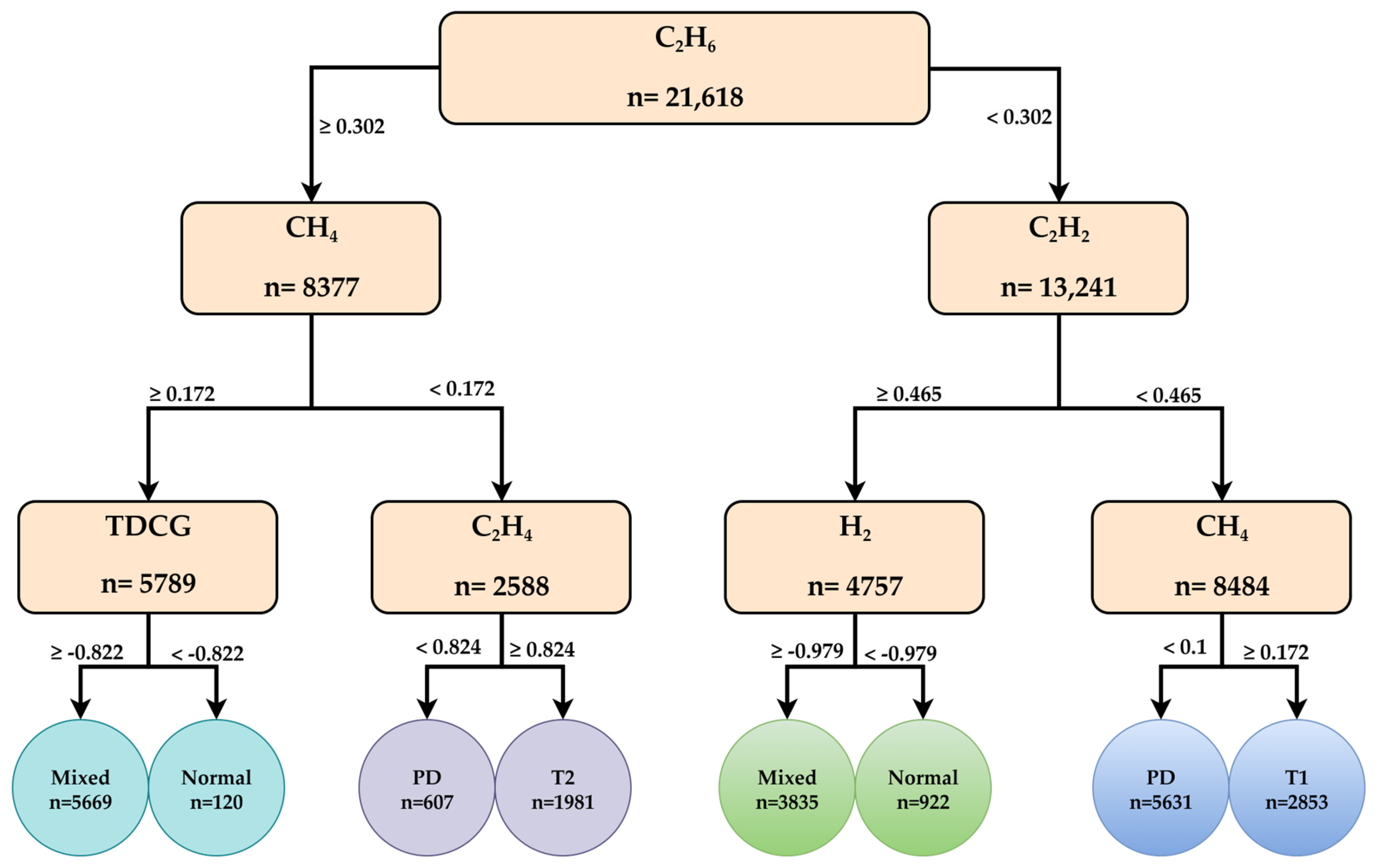
Figure 7 shows the final decision tree used to identify transformer faults, highlighting where gases are divided, the cutoff values, and the predicted fault types at the end points.

The diagram shows that C₂H₆, C₂H₂, CH₄, and H₂ are the main gases in the first divisions, matching the combined classification rules that set cutoff values of 280–300 for C₂H₆, 0.5–1.0 for C₂H₂, and 200–300 for H₂. These results are well supported by the literature, as many studies have shown that decision trees work well for transformer fault classification using DGA and consistently find C₂H₆, C₂H₂, CH₄, and H₂ as important diagnostic gases [57,58].

The tree structure shows that mixed faults are often predicted when several limits are passed, like high levels of C₂H₆ and CH₄. On the other hand, normal conditions are found at lower amounts of CH₄ and H₂. This result confirms that the decision tree follows the same logic as the rule-based system and offers statistical proof. The cutoff points for C₂H₂ at 0.465 and CH₄ at 0.172 exactly match the known fault rule limits, supporting their use in automatic classification. The figure clearly shows how these limits work and supports the combined system. Several studies have shown that decision trees can distinguish normal conditions, heat faults, and electrical discharge types, which supports the described mixed fault classification ability [30,36].

5. Discussion

The proposed SGDT framework demonstrated that statistically derived DGA fault classification rules can be effectively integrated with Decision Tree learning for transformer fault identification. This framework can be expanded to include more condition monitoring data, like partial discharge, insulation damage, and Sweep Frequency Response Analysis (SFRA) measurements, as long as this data comes from the same transformer and covers the same monitoring time.

5.1. Role of Statistical Measures in Threshold Definition

The combined results from the statistical analysis and decision tree model confirm the effectiveness of the proposed hybrid method for transformer fault classification using DGA. The statistical analysis showed consistent patterns in how key gases behave. Gases like H₂, CH₄, C₂H₂, and C₂H₆ were closely linked to certain fault types. These findings support using percentile-based limits to better detect faults. Earlier studies have examined different statistical patterns to analyse DGA data and create local rules for fault detection [59].

Table 16. Summary of statistical measures and their roles in fault threshold definition and classification.

Measure	Explanation
Median	Used to anchor normal gas behaviour; several thresholds (e.g., H2 = 336.8) are set below or above the median to detect abnormal levels.
Mean	Confidence intervals around the mean confirm the statistical reliability of threshold positioning.
Sum	Used to show total gas levels, especially for TDCG, to reflect overall gas buildup. Not directly used for rule limits, but helps assess severity.
Standard Deviation	Used to measure gas changes and choose limits that exceed normal variation.
CV	Useful for showing relative differences, especially for gases like C2H2 where the actual amounts are small but changes are important.
IQR	Important for setting percentile-based limits, especially for H2, C2H6, and C2H4.
Variance	Looked at together with standard deviation to highlight differences, especially for C2H6 and TDCG.
Range	Used to identify common gases (e.g., C2H6) and help set limits for thermal faults.
Minimum and Maximum	Used to check limit values (for example, C2H4 max = 26.8) and find data quality problems by spotting negative minimum values.
Percentiles (25th, 75th, 95th)	Directly support percentile-based rule thresholds (e.g., C2H2 95th = 0.41).
Skewness and Kurtosis	Used to confirm distribution shapes and risks of extreme values that influence the sensitivity and robustness of selected thresholds.
Covariance	Used to identify co-occurrence of gases in magnitude, supporting grouping of gases in rules (e.g., H2–C2H6, CH4–C2H6) and understanding direction and intensity of joint gas behaviour.
Pearson Correlation	Applied to confirm linear relationships, support, or validate combinations of gases in fault rules (e.g., CH4 and CO for thermal rules), and isolate independent gases like C2H2.

shows the statistical measures used in this study and explains how they help set limits based on data and guide fault classification.

Measures such as IQR and CV allowed for robust threshold setting, particularly for gases like C₂H₂, which showed high relative variability. Correlation and covariance analyses further confirmed strong interdependencies among thermal-related gases, especially between CH₄, C₂H₆, and CO, justifying their combined use in fault rules, as is also confirmed in the studies [60,61].

5.2. Model-Based Validation of Rule-Based Classification

The decision tree model showed these results by learning rules that matched the IEC and IEEE standards. The places where the data was split and the order of variables matched the combined limits, like CH₄ at 0.172 and C₂H₂ at 0.465. These results show that the model copied the expert-set limits, reaching 99.3% accuracy and F1 scores over 0.98. Using different methods, as shown in [62,63,64], multiple studies have reported high classification accuracies, with some achieving similar accuracy and F1 scores to those reported in this work.

Feature importance analysis indicated that H₂, CH₄, and C₂H₆ contributed most significantly to model accuracy, which aligns with findings from previous studies [65,66,67].

Table 17. Validation of rule-based fault classification using a decision tree model.

Aspect	Model Evidence Supporting Rules and Standards
Accuracy	High test accuracy (99.3%) confirms correct and consistent rule-based fault labelling.
Validity	Model divisions matched set statistical limits (e.g., C2H2 = 0.465, CH4 = 0.172, H2 = 300), confirming fault rules.
Reliability	Similar F1 scores for all groups (average = 0.98) show that the rules work reliably across all parts of the data.
Credibility	The main gases (H2, CH4, TDCG, C2H2, C2H6) match the diagnostic gases used by IEC and IEEE and follow rules made by experts.
Exclusion Support	The small effect of CO2, O2, H2O, and TDCG rate supports leaving them out of rules based on set limits.
Model Validation Role	Confirms that the rule-based classification system is supported by statistics, matches the data, and can be checked using ML.

summarises how the decision tree model confirmed the accuracy, reliability, and relevance of the statistical thresholds used in the rule-based fault classification.

The claimed 99.3% accuracy outperforms most comparable models in the literature, though the margin varies significantly across studies, as

Table 18. Comparative performance of transformer fault diagnosis models from the literature and the proposed hybrid model.

Ref. No.	Model/Method	Type/Approach	Reported Accuracy (%)
Current study	Proposed Model	Hybrid statistical + decision tree	99.3
[30]	Decision Tree (Duval Triangle-based)	Hybrid rule + ML	98
[36]	J48 Algorithm	Decision tree	81
[68]	Decision Tree (Duval Pentagon integration)	Hybrid rule + ML	91.84
[69]	Probabilistic Neural Network (PNN)	ML	98.28
[70]	Duval Triangle	Conventional DGA rule-based	87.18
	Neural Network	ML	97.9
	Support Vector Machine (SVM)	ML	95.7

shows.

Based on the available sources, the 99.3% accuracy and F1 scores above 0.98 exceed those of several benchmark studies. Decision tree methods gave different results: 81% for J48 algorithms, 98% for Duval Triangle-based models, and 91.84% for Duval Pentagon integration [68]. Probabilistic neural networks had a similar result of 98.28% [69]. The main features found (H₂, CH₄, C₂H₆) match what is known from other studies, which supports the model’s reliability. Traditional diagnostic methods worked less well, with the Duval Triangle only reaching 87.18% accuracy [70]. On the other hand, ML methods like neural networks (97.90%) and SVMs (95.70%) showed better accuracy. Table 18 shows a comparison of transformer fault diagnosis models from past studies and the new hybrid model.

6. Conclusions

The proposed SGDT framework, which combined advanced statistics applications together with decision tree learning, was accurate and reliable at identifying faults with real-world DGA transformer data. The results reached an accuracy of 99.3%, precision of 0.981, recall of 0.980, F1-score of 0.980, and AUC of 0.987, showing excellent prediction, balanced classification, and strong separation between fault types. Testing with 33,778 operational DGA records showed that this method provided a simple, statistically based, and widely useful tool for checking transformer condition. The results showed that the method improved fault detection, helped spot problems early, and supported better transformer health management and maintenance decisions.

Although the hybrid model worked well, a few issues remain and should be explored in future work: first, negative gas values were found in the data. This shows a need for better data checks before analysis. Secondly, only linear relationships were studied in this work. Therefore, more advanced models may help detect complex fault signs. Thirdly, the method was tested on one dataset; therefore, the proposal is that the same method should be applied to more transformers under different conditions, such as age, load history, geographical location, and maintenance practices. Furthermore, future work will consider stray gassing cases, and other parameters that may be effective for fault detection.

References

1. Lebedev, V. Transformer Basics. In Proceedings of the 2007 Electrical Insulation Conference and Electrical Manufacturing Expo, Nashville, TN, USA, 22–24 October 2007; pp. 356–359. [Google Scholar]
2. Werle, P.; Brendel, H. Transformers. In Springer Handbooks; Springer: Singapore, 2021; pp. 443–509. ISBN 9789813299375. [Google Scholar]
3. Metwally, I.A. Failures, Monitoring and New Trends of Power Transformers. IEEE Potentials 2011, 30, 36–43. [Google Scholar] [CrossRef] [Scilit]
4. Rampersad, R.M.; Bahadoorsingh, S.; Sharma, C. Multifactorial Frameworks Modelling Linkages of Power Transformer Fail Ure Modes. In Proceedings of the 2018 IEEE Electrical Insulation Conference (EIC), San Antonio, TX, USA, 17–20 June 2018; pp. 398–402. [Google Scholar] [CrossRef] [Scilit]
5. Arshad, M.; Islam, S.M.; Khaliq, A. Power Transformer Asset Management. In Proceedings of the 2004 International Conference on Power System Technology, Singapore, 21–24 November 2004; Volume 2, pp. 1395–1398. [Google Scholar] [CrossRef] [Scilit]
6. Gockenbach, E.; Borsi, H. Condition Monitoring and Diagnosis of Power Transformers. In Proceedings of the 2008 International Conference on Condition Monitoring and Diagnosis, Beijing, China, 21–24 April 2008; pp. 894–897. [Google Scholar]
7. Dupuis, B. An Introduction to Electrical Diagnostic Testing of Power Transformers. IEEE Power Energy Mag. 2016, 14, 38–45. [Google Scholar] [CrossRef] [Scilit]
8. Nafar, M.; Bahmani-Firouzi, B.; Jabbari, M. Transformer Monitoring by Using Vibration Analysis. Aust. J. Basic Appl. Sci. 2011, 5, 984–990. [Google Scholar]
9. Abu Bakar, N.; Abu-Siada, A. High Voltage Power Transformer Dissolved Gas Analysis, Measurement and Interpretation Techniques. High Volt. Maint. Forum 2013, 2008, 1–17. [Google Scholar]
10. Ali, M.S.; Abu Bakar, A.H.; Omar, A.; Abdul Jaafar, A.S.; Mohamed, S.H. Conventional Methods of Dissolved Gas Analysis Using Oil-Immersed Power Transformer for Fault Diagnosis: A Review. Electr. Power Syst. Res. 2023, 216, 109064. [Google Scholar] [CrossRef] [Scilit]
11. Taha, I.B.M.; Hoballah, A.; Ghoneim, S.S.M. Optimal Ratio Limits of Rogers’ Four-Ratios and IEC 60599 Code Methods Using Particle Swarm Optimization Fuzzy-Logic Approach. IEEE Trans. Dielectr. Electr. Insul. 2020, 27, 222–230. [Google Scholar] [CrossRef] [Scilit]
12. Suwarno; Sutikno, H.; Prasojo, R.A.; Abu-Siada, A. Machine Learning Based Multi-Method Interpretation to Enhance Dissolved Gas Analysis for Power Transformer Fault Diagnosis. Heliyon 2024, 10, e25975. [Google Scholar] [CrossRef] [Scilit] [PubMed]
13. Gouda, O.E.; El-Hoshy, S.H.; Ghoneim, S.S.M. Enhancing the Diagnostic Accuracy of DGA Techniques Based on IEC-TC10 and Related Databases. IEEE Access 2021, 9, 118031–118041. [Google Scholar] [CrossRef] [Scilit]
14. Soni, R.; Chaudhari, K. An Approach to Diagnose Incipient Faults of Power Transformer Using Di Ssolved Gas Analysis of Mineral Oil by Ratio Methods Using Fuzzy Logic. In Proceedings of the 2016 International Conference on Signal Processing, Communication, Power and Embedded System (SCOPES), Paralakhemundi, India, 3–5 October 2016; pp. 1894–1899. [Google Scholar] [CrossRef] [Scilit]
15. Abu-Siada, A. Improved Consistent Interpretation Approach of Fault Type within Power Transformers Using Dissolved Gas Analysis and Gene Expression Program Ming. Energies 2019, 12, 730. [Google Scholar] [CrossRef] [Scilit]
16. Hechifa, A.; Labiod, C.; Lakehal, A.; Nanfak, A.; Mansour, D.-E.A. A Novel Graphical Method for Interpretating Dissolved Gases and Fault Diagnosis in Power Transformer Based on Dynamique Axes in Circular For M. IEEE Trans. Power Deliv. 2024, 39, 3186–3198. [Google Scholar] [CrossRef] [Scilit]
17. Mosinski, F.; Piotrowski, T. New Statistical Methods for Evaluation of DGA Data. IEEE Trans. Dielectr. Electr. Insul. 2003, 10, 260–265. [Google Scholar] [CrossRef]
18. Tra, V.; Duong, B.-P.; Kim, J.-M. Improving Diagnostic Performance of a Power Transformer Using an Adaptive Over-Sampling Method for Imbalanced Data. IEEE Trans. Dielectr. Electr. Insul. 2019, 26, 1325–1333. [Google Scholar] [CrossRef] [Scilit]
19. Mahmoudi, N.; Samimi, M.H.; Mohseni, H. Experiences with Transformer Diagnosis by DGA: Case Studies. IET Gener. Transm. Distrib. 2019, 13, 5431–5439. [Google Scholar] [CrossRef] [Scilit]
20. Mashifane, L.D.; Mendu, B.; Monchusi, B.B. State-of-the-Art Fault Detection and Diagnosis in Power Transformers: A Review of Machine Learning and Hybrid Methods. IEEE Access 2025, 13, 48156–48172. [Google Scholar] [CrossRef] [Scilit]
21. Rao, S.U.M.; Babu, V.R.; Divya, C.H.; Naidu, C.R.; Moses, G.J.; Lakshmanarao, A. A Novel Approach to DGA Detection Combining Machine Learning and Transformer-Based Techniques. In Proceedings of the 2024 International Conference on IoT Based Control Networks and Intelligent Systems (ICICNIS), Bengaluru, India, 17–18 December 2024; pp. 1416–1420. [Google Scholar]
22. Gogoi, B.; Ahmed, T. DGA Domain Detection Using Pretrained Character Based Transformer Models. In Proceedings of the 2023 IEEE Guwahati Subsection Conference (GCON), Guwahati, India, 23–25 June 2023; pp. 1–6. [Google Scholar]
23. Yang, C.; Lu, T.; Yan, S.; Zhang, J.; Yu, X. N-Trans: Parallel Detection Algorithm for DGA Domain Names. Future Internet 2022, 14, 209. [Google Scholar] [CrossRef] [Scilit]
24. Anderson, H.S.; Woodbridge, J.; Filar, B. DeepDGA: Adversarially-Tuned Domain Generation and Detection. In Proceedings of the 2016 ACM Workshop on Artificial Intelligence and Security, Vienna, Austria, 28 October 2016; pp. 13–21. [Google Scholar]
25. Stampar, M.; Fertalj, K. Applied Machine Learning in Recognition of DGA Domain Names. Comput. Sci. Inf. Syst. 2022, 19, 205–227. [Google Scholar] [CrossRef] [Scilit]
26. Yu, B.; Gray, D.L.; Pan, J.; De Cock, M.; Nascimento, A.C.A. Inline DGA Detection with Deep Networks. In Proceedings of the 2017 IEEE International Conference on Data Mining Workshops (ICDMW), New Orleans, LA, USA, 18–21 November 2017; pp. 683–692. [Google Scholar]
27. Morbidoni, C.; Spalazzi, L.; Teti, A.; Cucchiarelli, A. Leveraging N-Gram Neural Embeddings to Improve Deep Learning DGA Detection. In Proceedings of the 37th ACM/SIGAPP Symposium on Applied Computing, Virtual Event, 25–29 April 2022; ACM: New York, NY, USA, 2022; pp. 995–1004. [Google Scholar]
28. Kahlen, J.N.; Andres, M.; Moser, A. Improving Machine-Learning Diagnostics with Model-Based Data Augmentat Ion Showcased for a Transformer Fault. Energies 2021, 14, 6816. [Google Scholar] [CrossRef] [Scilit]
29. Leite, D.; Andrade, E.; Rativa, D.; Maciel, A.M.A. Fault Detection and Diagnosis in Industry 4.0: A Review on Challenges and Opportunities. Sensors 2024, 25, 60. [Google Scholar] [CrossRef] [Scilit]
30. Olowolafe, F.; Alawode, K.O. Detection of Incipient Faults in Power Transformers Using Fuzzy Logic and Decision Tree Models Based on Dissolved Gas Analysis. ABUAD J. Eng. Res. Dev. (AJERD) 2024, 7, 56–73. [Google Scholar] [CrossRef] [Scilit]
31. Shahrabad, S.J.T.; Ghods, V.; Askari, M.T. Power Transformer Fault Diagnosis Using DGA and Artificial Intelligence. Recent Adv. Comput. Sci. Commun. 2019, 13, 579–587. [Google Scholar] [CrossRef] [Scilit]
32. Moradi, E.; Mahmoud, K.; Darwish, M.M.F. Advanced Ensemble Learning Classifiers for Power Transformer Fault Diagnosis with Imbalanced DGA Data. In Proceedings of the 25th International Middle East Power System Conference (MEPCON), Cairo, Egypt, 17–19 December 2024; pp. 1–5. [Google Scholar] [CrossRef] [Scilit]
33. Odongo, G.; Musabe, R.; Hanyurwimfura, D. A Multinomial DGA Classifier for Incipient Fault Detection in Oil-Impregnated Power Transformers. Algorithms 2021, 14, 128. [Google Scholar] [CrossRef] [Scilit]
34. Huang, H. Fault Diagnosis of Transformers Based on Gbdt Method. In Proceedings of the 2025 6th International Conference on Artificial Intelligence and Electromechanical Automation (AIEA), Hefei, China, 1–3 August 2025. [Google Scholar] [CrossRef] [Scilit]
35. Basuki, A. Suwarno Online Dissolved Gas Analysis of Power Transformers Based on Decision Tree Model. In Proceedings of the 2018 Conference on Power Engineering and Renewable Energy (ICPERE), Solo, Indonesia, 29–31 October 2018; pp. 1–6. [Google Scholar] [CrossRef] [Scilit]
36. Bakar, N.A.; Chairul, I.S.; Ghani, S.A.; Ahmad Khiar, M.S.; Che Wanik, M.Z. Improvement of Transformer Dissolved Gas Analysis Interpretation Using J48 Decision Tree Model. IAES Int. J. Artif. Intell. (IJ-AI) 2023, 12, 48. [Google Scholar] [CrossRef] [Scilit]
37. Menezes, A.G.C.; Almeida, O.M.; Barbosa, F.R. Use of Decision Tree Algorithms to Diagnose Incipient Faults in Power Transformers. In Proceedings of the 2018 Simposio Brasileiro de Sistemas Eletricos (SBSE), Niteroi, Brazil, 12–16 May 2018; pp. 1–6. [Google Scholar] [CrossRef] [Scilit]
38. Menezes, A.G.C.; Araujo, M.M.; Almeida, O.M.; Barbosa, F.R.; Braga, A.P.S. Induction of Decision Trees to Diagnose Incipient Faults in Power Tran Sformers. IEEE Trans. Dielectr. Electr. Insul. 2022, 29, 279–286. [Google Scholar] [CrossRef] [Scilit]
39. Hechifa, A.; Lakehal, A.; Labiod, C.; Nanfak, A.; Mansour, D.-E.A.; Said, D. The Effect of Source Data on Graphical Pentagons DGA Methods for Detecting Incipient Faults in Power Transformers. In Proceedings of the 2023 International Conference on Decision Aid Sciences and Applications (DASA), Annaba, Algeria, 16–17 September 2023; pp. 152–157. [Google Scholar]
40. Nanfak, A.; Hechifa, A.; Eke, S.; Lakehal, A.; Kom, C.H.; Ghoneim, S.S.M. A Combined Technique for Power Transformer Fault Diagnosis Based on k-means Clustering and Support Vector Machine. IET Nanodielectr. 2024, 7, 175–187. [Google Scholar] [CrossRef] [Scilit]
41. Merita, A.K.; Sharma, R.N.; Chauhan, S. Study and Diagnosis of Key Gases to Assess Condition of Power Transformers. In Proceedings of the 2011 3rd International Conference on Electronics Computer Technology, Kanyakumari, India, 8–10 April 2011; pp. 343–347. [Google Scholar]
42. Kadim, E.J.; Hee, C.F.; Azis, N.; Jasni, J.; Ahmad, S.A.; Kadir, M.Z.A.A. Dissolved Gas Analysis of Transformers Based on Rough Set and Fuzzy Logic Methods. In Proceedings of the 2015 IEEE Conference on Energy Conversion (CENCON), Johor Bahru, Malaysia, 19–20 October 2015; pp. 268–271. [Google Scholar]
43. Chattranont, N.; Wannakarn, P.; Woothipatanapan, S.; Rugthaicharoencheep, N. Dissolved Gas Analysis of 115 KV Steel Industry Transformer Using New IEEE Standard. In Proceedings of the 2021 18th International Conference on Electrical Engineering/Electronics, Computer, Telecommunications and Information Technology (ECTI-CON), Chiang Mai, Thailand, 19–22 May 2021; pp. 603–606. [Google Scholar]
44. IEEE Std C57.104-2019; IEEE Guide for the Interpretation of Gases Generated in Mineral Oil-Immersed Transformers (Revision of IEEE Std C57.104-2008). IEEE: New York, NY, USA, 2019.
45. Duval, M.; dePabla, A. Interpretation of Gas-in-Oil Analysis Using New IEC Publication 60599 and IEC TC 10 Databases. IEEE Electr. Insul. Mag. 2001, 17, 31–41. [Google Scholar] [CrossRef] [Scilit]
46. Duval, M. Dissolved Gas Analysis and the Duval Triangle. In Proceedings of the TechCon Asia Pacific, Sydney, Australia, 6–8 December 2006; pp. 1–20. [Google Scholar]
47. Zhou, D.; Azis, N.; Yang, G.Y.; Wang, Z.D.; Jones, D.; Wells, B.; Wallwork, G.M. Examining Acceptable Dissolved Gas Analysis Level of In-Service Transformers. In Proceedings of the 2012 International Conference on High Voltage Engineering and Application, Shanghai, China, 17–20 September 2012; pp. 612–616. [Google Scholar]
48. Junfithrana, A.P.; Hakim, L.; Nopiyanti, R.; Muslih, M. Improving TDGC on Oil Dissolved Tranformator Gas Using Fuzzy Logic. In Proceedings of the 2020 6th International Conference on Computing Engineering and Design (ICCED), Sukabumi, Indonesia, 15–16 October 2020; IEEE: New York, NY, USA, 2020; pp. 1–6. [Google Scholar]
49. Siswanto, A.; Rohman, A.; Suprijadi, S.; Baehaqi, M.; Arifudin, A. Analisis Karakteristik Minyak Transformator Menggunakan Pengujian Dissolved Gas Analysis (DGA) Pada IBT 1 Gardu Induk. Foristek 2022, 12, 30–42. [Google Scholar] [CrossRef] [Scilit]
50. Semanjski, I.C. Data Analytics. In Smart Urban Mobility; Elsevier: Amsterdam, The Netherlands, 2023; pp. 121–170. ISBN 978-0-12-820717-8. [Google Scholar]
51. Yedidia, A.B. Against the F-Score. 2016, 1–14. Available online: https://adamyedidia.wordpress.com/wp-content/uploads/2014/11/f_score.pdf (accessed on 21 August 2026).
52. Molina, M. Un Intruso de Otro Mundo: F1-Score. Rev. Electrón. AnestesiaR 2024, 16, 3. [Google Scholar] [CrossRef] [Scilit]
53. Lipton, Z.C.; Elkan, C.; Narayanaswamy, B. Thresholding Classifiers to Maximize F1 Score. arXiv 2014, arXiv:1402.1892. [Google Scholar]
54. Zhang, D.; Wang, J.; Zhao, X. Estimating the Uncertainty of Average F1 Scores. In Proceedings of the 2015 International Conference on The Theory of Information Retrieval, Northampton, MA, USA, 27–30 September 2015; ACM: New York, NY, USA, 2015; pp. 317–320. [Google Scholar]
55. Takahashi, K.; Yamamoto, K.; Kuchiba, A.; Shintani, A.; Koyama, T. Hypothesis Testing Procedure for Binary and Multi-class F1 -scores in the Paired Design. Stat. Med. 2023, 42, 4177–4192. [Google Scholar] [CrossRef] [Scilit]
56. Sazzed, S.; Scheible, P.; Alshammari, M.; Wriggers, W.; He, J. Cylindrical Similarity Measurement for Helices in Medium-Resolution Cr Yo-Electron Microscopy Density Maps. J. Chem. Inf. Model. 2020, 60, 2644–2650. [Google Scholar] [CrossRef] [Scilit]
57. Raj, R.A.; Sarathkumar, D.; Venkatachary, S.K.; Andrews, L.J.B. Classification and Prediction of Incipient Faults in Transformer Oil by Supervised Machine Learning Using Decision Tree. In Proceedings of the 2023 3rd International conference on Artificial Intelligence and Signal Processing (AISP), Vijayawada, India, 18–20 March 2023; pp. 1–6. [Google Scholar] [CrossRef] [Scilit]
58. Liu, C.-H.; Chen, T.-L.; Yao, L.-T.; Wang, S.-Y. Using Data Mining to Dissolved Gas Analysis for Power Transformer Fault Diagnosis. In Proceedings of the 2012 International Conference on Machine Learning and Cybernetics; International Conference on Machine Learning and Cybernetics, Xi’an, China, 15–17 July 2012; pp. 1952–1957. [Google Scholar] [CrossRef] [Scilit]
59. Zhao, C.; Huang, Q.; Li, D.; Bai, H.; Cheng, Y. The Statistical Distribution of the DGA Data of Transformers and Its Application. In Proceedings of the 2016 IEEE International Conference on Dielectrics (ICD), Montpellier, France, 3–7 July 2016; Volume 1, pp. 497–500. [Google Scholar]
60. Dhole, V.; Kadam, V. Advantages of the TOGA-Transformer Oil Gas Analyzer Involving Headspace-GC Analysis and a DGA System. Appl. Note 2012, 10348, 1–6. [Google Scholar]
61. Zhao, A.-X.; Tang, X.-J.; Zhang, Z.-H.; Liu, J.-H. The DGA Interpretation Method Using Relative Content of Characteristic Gases and Gas-Ratio Combinations for Fault Diagnosis of Oil-Immersed Power Transformers. In Proceedings of the 2014 International Symposium on Electrical Insulating Materials, Niigata, Japan, 1–5 June 2014; pp. 124–127. [Google Scholar]
62. Aburaghiega, E.; Emad Farrag, M.; Hepburn, D.M.; Garcia, B. Enhanced Condition Monitoring of Power Transformers through Improvement in Accuracy of DGA Interpretation. In Proceedings of the 2016 51st International Universities Power Engineering Conference (UPEC), Coimbra, Portugal, 6–9 September 2016; pp. 1–6. [Google Scholar]
63. Wani, S.A.; Gupta, D.; Farooque, M.U.; Khan, S.A. Multiple Incipient Fault Classification Approach for Enhancing the Acc Uracy of Dissolved Gas Analysis (DGA). IET Sci. Meas. Technol. 2019, 13, 959–967. [Google Scholar] [CrossRef] [Scilit]
64. Al-Sakini, S.R.; Bilal, G.A.; Sadiq, A.T.; Al-Maliki, W.A.K. Dissolved Gas Analysis for Fault Prediction in Power Transformers Usin g Machine Learning Techniques. Appl. Sci. 2024, 15, 118. [Google Scholar] [CrossRef] [Scilit]
65. Raj, R.A.; Murugesan, S.; Sarathkumar, D.; Venkatachary, S.K.; Andrews, L.J.B. Investigating the Survival and Hazards of Dissolved Gases in Transformer Oil Using DGA History. In Proceedings of the 2023 IEEE 12th International Conference on Communication Systems and Network Technologies (CSNT), Bhopal, India, 8–9 April 2023; pp. 934–939. [Google Scholar]
66. Chanchotisatien, P.; Vong, C. Feature Engineering and Feature Selection for Fault Type Classification from Dissolved Gas Values in Transformer Oil. In Proceedings of the 2021 25th International Computer Science and Engineering Conference (ICSEC), Chiang Rai, Thailand, 18–20 November 2021; pp. 75–80. [Google Scholar]
67. Hashemi, M.H. Applications of Feature Selection for Detecting Energy Discharge and Thermal Faults in Transformers Using DGA Data. In Proceedings of the 2024 8th International Artificial Intelligence and Data Processing Symposium (IDAP), Malatya, Turkiye, 21–22 September 2024; Volume 29, pp. 1–5. [Google Scholar]
68. Manimala, R.; Vigneshwaran, B. Enhanced Fault Diagnosis in Transformer Oil Using Duval Pentagon Method. In Proceedings of the 2025 5th International Conference on Expert Clouds and Applications (ICOECA), Bengaluru, India, 6–7 March 2025; pp. 385–389. [Google Scholar]
69. Malik, H.; Mishra, S. Feature Selection Using RapidMiner and Classification through Probabilistic Neural Network for Fault Diagnostics of Power Transformer. In Proceedings of the 2014 Annual IEEE India Conference (INDICON), Pune, India, 11–13 December 2014; pp. 1–6. [Google Scholar]
70. Tan, J.P.; Jueco, J.C.; Tan, E.M. Performance Analysis of Multiple Machine Learning Models Applied to Dissolved Gas Analysis Under Thermal Fault Classification Considering IEEE C57.104-2019TM Standard for Substation Transformer. In Proceedings of the 2024 FORTEI-International Conference on Electrical Engineering (FORTEI-ICEE), Badung, Indonesia, 24–25 October 2024; pp. 247–252. [Google Scholar]
Figure 1. Workflow of the proposed Statistically Guided Decision Tree (SGDT) framework for transformer fault classification.
Energies 19 03986 g001
Figure 2. Distribution characteristics of transformer DGA variables.
Energies 19 03986 g002
Figure 3. Correlation heatmap of key dissolved gases.
Energies 19 03986 g003
Figure 4. Relative importance of predictor variables for transformer fault classification.
Energies 19 03986 g004
Figure 5. ROC curve plot for multi-class transformer fault type classification.
Energies 19 03986 g005
Figure 6. How classification accuracy changes for training and validation sets with different levels of complexity penalty.
Energies 19 03986 g006
Figure 7. Visual representation of the decision tree used to classify transformer fault types.
Energies 19 03986 g007