Hub-Height Optimization of Offshore Wind Farm Based on the Tian Ji’s Horse Racing Algorithm and Collaborative Staggering Layout Considering Primary and Secondary Wind Directions

Abstract

In offshore wind farm micro-siting, maximizing annual power generation across all wind directions often involves a trade-off among different directional conditions, especially when the primary and secondary wind directions account for most wind energy. To address this issue, this paper proposes a turbine layout strategy combining horizontal and vertical staggering. The objective function maximizes the simplified capital efficiency (power generation per unit capital cost) under the primary and secondary wind directions, for which a layout optimization model is constructed and solved using the Tian Ji’s Horse Racing Algorithm (THRO). A case study on an offshore wind farm validates the proposed approach. Results show that, compared with manual empirical layout and the GA-PSO algorithm, the proposed strategy significantly improves the simplified capital efficiency under the primary and secondary wind directions, while also enhancing overall power generation efficiency across all wind directions. This offers a new technical pathway for offshore wind farm micro-siting. Additionally, the THRO algorithm converges within 30 iterations, outperforming conventional optimization algorithms and demonstrating its effectiveness in solving such optimization problems.

1. Introduction

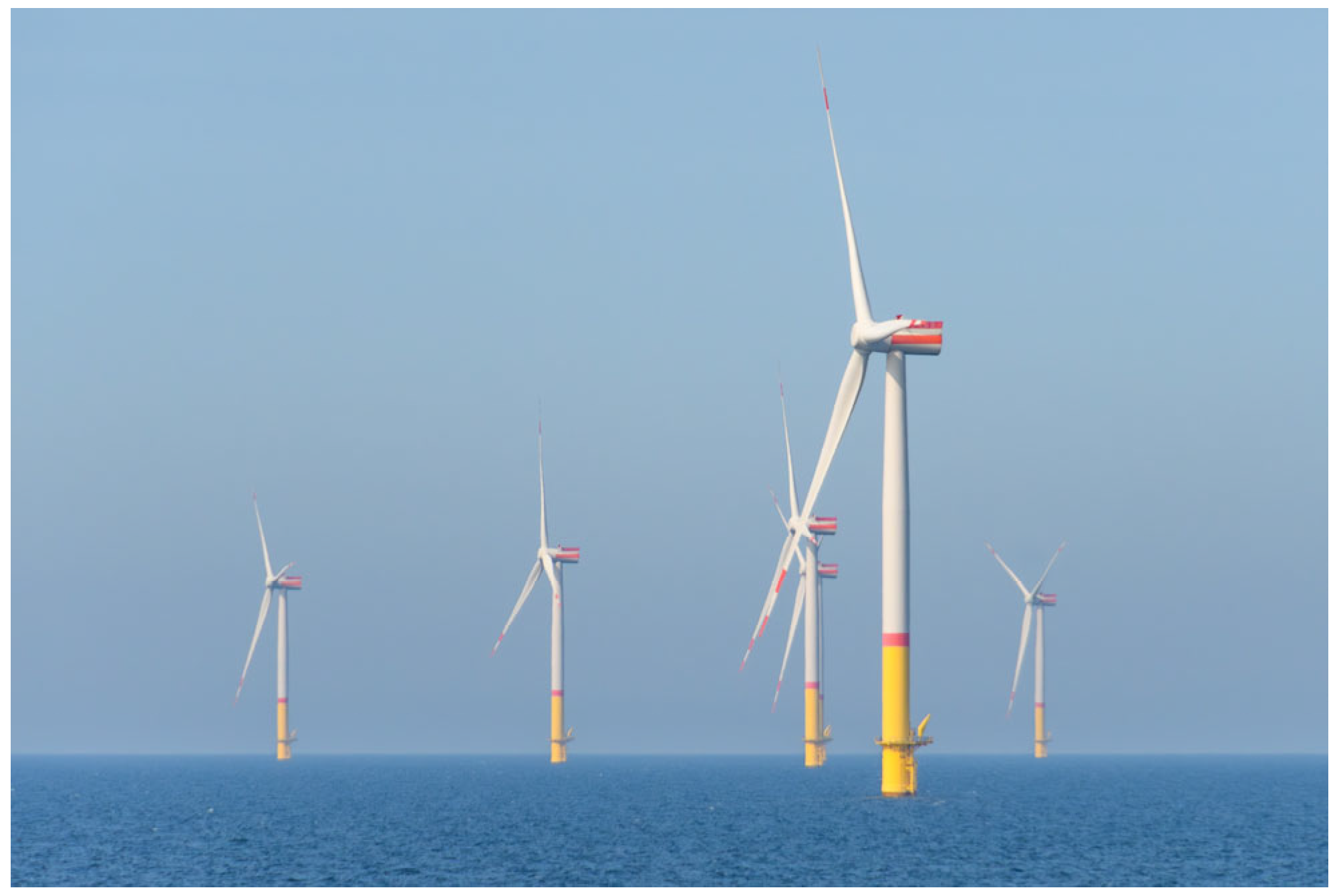
With the continuous growth in electricity demand, the non-renewable nature of traditional fossil energy and its environmental impacts have made the development and utilization of renewable energy a major trend in the energy sector. In recent years, wind power technology in China has become increasingly mature, with a steadily expanding scale of deployment. Among various renewable energy sources, offshore wind energy has become one of the primary directions for wind power development due to its abundant and stable resources, lower wind shear, proximity to load centers, and minimal occupation of land resources [1]. Recent studies have also investigated the integration of offshore wind with other systems [2], further highlighting its potential in the energy transition. However, offshore wind farms are constrained by limited available sea space. In addition, low turbulence intensity and slow wake recovery result in greater wake losses compared with onshore wind farms, making micro-siting (i.e., the optimal arrangement of wind turbines) crucial for improving power generation efficiency and capital efficiency. Therefore, the question of how to achieve an efficient and scientific turbine layout optimization has become a key issue that urgently needs to be addressed in offshore wind energy development. Figure 1 shows a typical offshore wind farm.

Wind turbine layout strategies primarily involve two aspects: the staggered arrangement of turbines and the determination of the primary wind direction. Research on staggered layout strategies has focused on two dimensions, namely, horizontal staggering and vertical staggering. Since the pioneering work of Reference [3] on offshore wind farm micro-siting, numerous studies have concentrated on horizontal layout optimization. Moreover, the influence of wind shear on wake effects has prompted many researchers to investigate vertical staggering among wind turbines [4]. By assigning different hub heights, a vertical distance can be imposed between adjacent turbines, providing an alternative means to more efficiently utilize wind energy resources and limited sea areas. Reference [5] investigated the feasibility of applying two different hub heights to turbines arranged in a straight line, and the results indicated that using wind turbines with varying hub heights may contribute to higher power output. Reference [6] examined the impact of vertical arrangement on wind farm power output, and the findings showed that when the hub height of some turbines was reduced from 78 m to 50 m, the overall power output of the wind farm increased. In staggered layouts, the determination of certain parameters, such as the staggering spacing, requires the selection of an appropriate wake model to quantify the influence of upstream turbines on downstream turbines. Therefore, the wake model constitutes one of the key aspects in the study of wind farm micro-siting layout schemes. Commonly used wake models include the Jensen model [7], the Gaussian model [8], computational fluid dynamics (CFD) simulations [9], and the FLORIS model [10]. These widely adopted models cover engineering analytical models, semi-analytical models, and high-fidelity numerical models. A significant trade-off exists among these models in terms of computational efficiency and accuracy: high-fidelity numerical models offer the highest accuracy but at a prohibitive computational cost; semi-analytical models strike a balance between computational complexity and accuracy; while engineering analytical models, despite their limited precision in capturing detailed wake characteristics, still demonstrate significant advantages in offshore wind farm layout optimization. Reference [11] compared onshore and offshore wind farm performance in the Baltic Sea using the Jensen wake model, finding that offshore achieves 1.5–1.7 times higher energy density but roughly 25% higher LCOE.

Optimization of wind farm layout under multi-wind-direction conditions has become a research consensus in this field. In the pioneering work on wind farm micro-siting [3], three wind condition scenarios were already considered, including a single wind direction, a constant wind speed with varying directions, and variations in both wind speed and direction. Subsequent studies have largely followed this approach, employing multi-directional sector partitioning for wind condition modeling and layout testing. Reference [12] particularly emphasized that wind direction discretization plays a critical role in wind farm layout optimization. Moreover, the influence of wind direction variation on power generation cannot be overlooked: Reference [13] employed a CFD method to simulate the power generation performance of a wind farm under all wind directions. The results indicate that a 20° deviation in wind direction can cause the total power output to fluctuate by up to 30%. To quantify this effect, Reference [14] introduced a wind-direction sensitivity index and proposed a layout optimization strategy that reduces sensitivity through local adjustments. Reference [15] took the Lillgrund offshore wind farm as the research object and employed the large-eddy simulation (LES) method to systematically quantify the sensitivity of wind farm performance to layout schemes. The results indicate that the power generation of the wind farm varies significantly under different inflow directions, and the performance of the layout scheme is closely related to the incoming wind direction.

The aforementioned studies indicate that wind direction variation exerts a significant influence on wind farm performance; nevertheless, the existing optimization frameworks still suffer from limitations in objective function formulation. Specifically, these limitations manifest in the fact that current studies typically adopt a single global objective, such as maximizing annual energy production (AEP) or minimizing levelized cost of energy (LCOE), as the optimization target. This practice implicitly presumes that the layout scheme must make a comprehensive trade-off across all wind directions without explicit prioritization among them, i.e., pursuing a compromise solution. Such an approach may constrain power generation in the primary wind direction. Studies have shown that when wind resources are relatively dispersed without a clearly primary direction, this type of all-direction comprehensive optimization tends to result in a relatively uniform dispersion of turbines across various sectors of the wind farm [16]. However, for wind farms characterized by a pronounced primary wind direction, the wind energy contribution from the primary direction often far exceeds that from other directions. Sacrificing the power generation potential of the primary direction for the sake of non-primary directions with lower energy density is economically questionable. Therefore, in wind farms with a clear primary wind direction, excessively pursuing an all-direction balanced layout may undermine the power generation potential in the primary direction and may not ultimately be conducive to maximizing annual energy production across all wind directions. In their study on the Lillgrund wind farm, Reference [15] observed that the actual wind rose exhibited a distinct two-sector characteristic, and therefore specifically adopted a two-sector wind rose in their optimization. This suggests that the all-direction comprehensive trade-off layout strategy is not necessarily optimal under all wind conditions.

Numerous studies have employed intelligent algorithms for offshore wind farm micro-siting optimization. The intelligent algorithms adopted include the genetic algorithm (GA) [17], particle swarm optimization (PSO) [18], and the GA-PSO hybrid algorithm [18], among others. Reference [19] proposed a genetic algorithm based on a bi-objective intelligent optimization model incorporating both profit margin and wind farm layout. Reference [20] introduced an improved genetic algorithm that combines binary encoding and real-number encoding, with annual energy production, construction cost, and wind energy utilization rate as the objective functions, thereby expanding the solution space of the micro-siting problem. Reference [3] optimized the turbine layout procedure and proposed a grid-based search algorithm using a genetic algorithm. Reference [21] developed an adaptive weight-based GA-PSO hybrid algorithm that integrates GA and PSO. Reference [22] developed a greedy algorithm to assign different tower heights and positions to wind turbines. Reference [23] developed an NPV-driven simulation-optimization framework that sequentially optimizes wind turbine design and farm layout, applied to two onshore sites in Egypt and Oman.

However, the aforementioned studies suffer from the following limitations: (1) In terms of layout strategies, only lateral offsets or longitudinal offsets are applied between adjacent turbines, i.e., wake effects are mitigated solely through either horizontal staggering or vertical staggering in isolation. (2) With regard to optimization objectives, if other wind directions contribute only marginally to the total AEP due to low energy density, compromising the performance of the primary direction for their sake may not be economically justified. (3) Concerning solution algorithms, the genetic algorithm is prone to premature convergence, while particle swarm optimization tends to suffer from diversity loss in the population during later stages, leading to search stagnation.

Based on the above analysis, this study proposes an alternative layout strategy: the optimization objective is set to maximize the simplified capital efficiency under the primary and secondary wind directions, aiming to perform targeted optimization on the directions with the highest energy density, thereby avoiding the inherent trade-off among directions in all-direction optimization. Furthermore, by integrating the identification of primary and secondary wind directions with a combined horizontal and vertical staggered layout, this study seeks to explore a novel layout paradigm for wind farms characterized by a wind rose with pronounced primary directions. The Tian Ji’s Horse Racing Optimization (THRO) algorithm is employed for solving the optimization problem. Inspired by the ancient Chinese fable of “Tian Ji’s Horse Racing,” this algorithm enables population individuals to adaptively select update strategies based on their current fitness levels through dual-population co-evolution and five dynamic competition strategies, thereby achieving flexible switching between global exploration and local refinement. Finally, simplified capital efficiency across all wind directions is adopted as a comprehensive performance evaluation metric to verify the effectiveness of the proposed strategy.

In this study, we focus on hub-height optimization for a fixed horizontal staggered layout, rather than optimizing turbine coordinates. This approach is motivated by the practical need to improve wind farm performance through vertical staggering while maintaining a regular horizontal arrangement. Finally, an offshore wind farm site is taken as the case study to conduct micro-siting optimization, with the aim of providing a reference for practical wind turbine layout.

2. Power Output Calculation of Wind Farms Considering Wake Effect

2.1. Fundamental Assumptions of the Jensen Wake Model

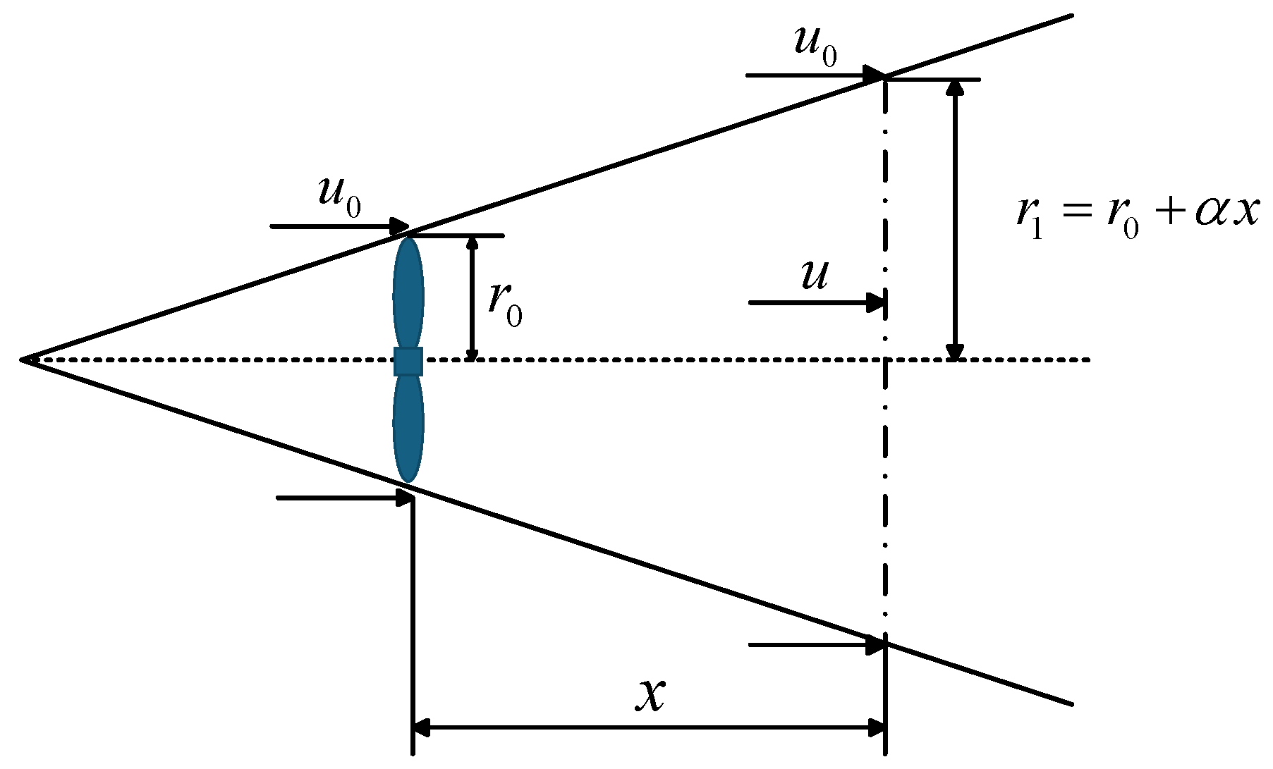
The marine environment is generally characterized by stable wind conditions, a near-neutral atmospheric boundary layer, low sea surface roughness, and the absence of complex terrain interference. These features are highly consistent with the assumptions of uniform steady inflow and neutral atmospheric stratification underlying the Jensen model. Moreover, the wake expansion behavior in such settings is primarily governed by ambient turbulence, and the linear expansion assumption has been well validated empirically in open sea areas. More importantly, large-scale offshore wind farms, particularly those in sea regions, require frequent calls to the wake model within the optimization algorithm for scheme evaluation during layout optimization. The Jensen model, with a single computation time on the order of microseconds, can significantly enhance design efficiency when embedded in large-scale optimization loops. Compared with onshore wind farms, offshore wind farms are characterized by much flatter terrain, and thus the Jensen wake model is sufficient for reliable simulation. A schematic diagram of the wake effect is shown in Figure 2.

The Jensen wake model relies on the following key assumptions:

(1) Uniform radial velocity distribution in the wake: it is assumed that the wind speed distribution at any cross-section within the wake region is uniform, i.e., a ‘top-hat’ velocity profile is adopted. In the Jensen wake model, the wake velocity distribution at a downstream distance $x$ is given by:

$$u(r)=\left\{\begin{array}{l}{u}_w,r\le R(x)\\ u_0,r>R(x)\end{array}\right.$$

(1)

where $u(r)$ denotes the wind speed at the wake boundary at the rotor plane; $u_w$ represents the wind speed within the wake cross-section; $u_0$ is the upstream wind turbine wind speed.

(2) Linear wake expansion: the wake influence radius increases linearly with the downstream distance from the turbine, and the expansion rate is determined by the wake decay coefficient. The wake influence radius is given by:

$$r_1=r_0+\alpha x$$

(2)

where $r_1$ denotes the wake influence radius at a downstream distance $x$; $r_0$ is the rotor blade radius; and α is the wake decay coefficient, which is calculated as follows:

$$\alpha ={\displaystyle \frac{0.5}{\ln (\frac{h}{z_0})}}$$

(3)

where $h$ denotes the hub height of the wind turbine; $z_0$ is the ground surface roughness, which is set to 0.04 in this study.

(3) Momentum conservation: pressure gradient effects are neglected during wake development, and the momentum deficit is assumed to be conserved as it propagates downstream. Under this assumption, the wind speed within the wake cross-section $u_w$ is derived as:

$$u_w=u_0[1-(1-\sqrt{1-C_T}{({\displaystyle \frac{r_0}{r_0+\alpha x}})}^2]$$

(4)

where $C_T$ denotes the thrust coefficient, which is typically obtained from the thrust coefficient curve provided by the turbine manufacturer.

These assumptions simplify the complex flow physics, making the model suitable for engineering applications. We acknowledge that this study adopts the neutral atmospheric stratification assumption inherent to the Jensen model, and does not explicitly account for the effects of atmospheric stability or turbulence intensity on wake recovery. This simplification is commonly accepted in engineering-level offshore wind farm layout optimization, though more refined models incorporating stability effects could be considered in future work.

The calculation of velocity deficit is the core component of the Jensen wake model, reflecting Assumption (3). This process can be specifically categorized into wake analysis for a single wind turbine and cumulative wake analysis for multiple turbines.

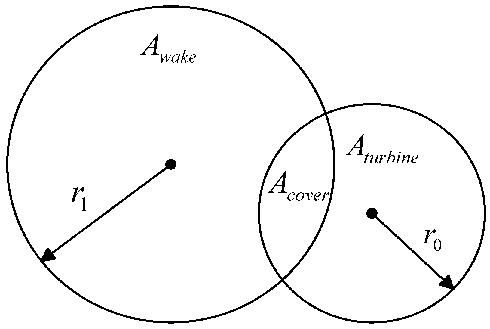
Depending on the relative positioning of upstream and downstream wind turbines, the impact of upstream wake effects on downstream turbines can be categorized into three scenarios: no wake overlap, partial wake overlap, and full wake overlap. For the latter two cases, it is necessary to calculate both the shadow area $A_{cover}$ and the wake region area $A_{wake}$ to determine the wake effect factor $A_{ratio}$. The calculation formula is as follows:

$$A_{ratio}={\displaystyle \frac{A_{cover}}{A_{wake}}}$$

(5)

Taking the partial overlap case as an example, the corresponding schematic diagram is shown in Figure 3.

As the partial wake overlap area gradually increases to complete overlap, the following condition is obtained: $A_{cover}=A_{turbine}$.

Accordingly, the wind speed at the downstream turbine affected by the upstream wake $u$ can be expressed as:

$$u=u_0[1-(1-\sqrt{1-C_T}{({\displaystyle \frac{r_0}{r_0+\alpha x}})}^2]A_{ratio}$$

(6)

However, downstream turbines in a wind farm are often affected by wakes from multiple upstream turbines, leading to wake superposition effects. The combined wake velocity is typically evaluated using the square root of the sum of squares of velocity deficits. The resulting wind speed at the downstream turbine location $u$ is given by:

$$u=u_0[1-\sqrt{{\displaystyle \sum _{i=1}^N{A}_{ratio,i}}{(1-{\displaystyle \frac{u_i}{u_0}})}^2}]$$

(7)

where $u_i$ denotes the wind speed at the downstream turbine after being affected by the wake of the i-th upstream turbine; the wake influence factor $A_{ratio,i}$ also corresponds to the i-th upstream turbine. It should be noted that in the implementation, the velocity deficit for each upstream turbine is first computed using Equation (6), which already incorporates the overlap ratio $A_{ratio}$ for that specific upstream–downstream pair. The squared deficits are then summed directly in Equation (7) without any additional multiplication by $A_{ratio}$. This ensures that the overlap effect is applied only once per upstream–downstream turbine pair and is not double-counted.

2.2. Annual Energy Production (AEP) of Wind Farms

The output power of a wind turbine is determined by the actual wind speed and its power characteristic curve. The actual wind speed depends on both turbine hub height and inter-turbine wake effects. Wind speeds at different heights are commonly estimated using the power law wind shear model, which can be expressed as:

$$u(h)=u_{ref}{({\displaystyle \frac{h}{h_{ref}}})}^{\beta }$$

(8)

where $u(h)$ denotes the effective wind speed at the turbine hub height $h$; $u_{ref}$ is the wind speed at the reference height $h_{ref}$; and $\beta$ is the wind shear exponent, which is set to 0.14 in this study.

The effect of hub height on power output is twofold. First, variations in hub height directly affect wind speed and thus power output. Second, increasing hub height reduces the wake decay coefficient, thereby indirectly affecting power output through wake effects, which is further analyzed based on the Jensen wake model established in Section 2.1.

After considering the effects of hub height and wake interactions, the actual wind speed can be obtained and then substituted into the power characteristic curve to calculate the output power of the corresponding wind turbine. The power curve is characterized by three key wind speed parameters: cut-in wind speed, rated wind speed, and cut-out wind speed, and its operating behaviors are typically expressed by a cubic function model:

$$P=\left\{\begin{array}{l}0,u_{ij}<u_{in} \mathrm{or} u_{ij}>u_{out}\\ P_{rate}{\left({\displaystyle \frac{u_{rate}-u_{ij}}{u_{rate}-u_{in}}}\right)}^3,u_{in}<u_{ij}<u_{rate}\\ P_{rate}, u_{rate}<u_{ij}<u_{out}\end{array}\right.$$

(9)

where $u_{ij}$ denotes the actual wind speed of the i-th turbine under the j-th wind resource dataset; $u_{in}$ is the cut-in wind speed; $u_{rate}$ is the rated wind speed; $u_{out}$ is the cut-out wind speed; and $P_{rate}$ is the rated power of the wind turbine. The operating characteristics of the wind turbine power curve can be described as follows: when the wind speed is below the cut-in wind speed, the turbine does not operate and the output power is zero. When the wind speed reaches or exceeds the cut-in wind speed but remains below the rated wind speed, the output power increases with wind speed. At the rated wind speed, the turbine produces its rated power. When the wind speed lies between the rated and cut-out wind speeds, the output power is regulated to remain constant at the rated level through power control strategies. When the wind speed exceeds the cut-out wind speed, the turbine is shut down for safety reasons, resulting in zero power output.

Finally, the theoretical annual energy production of the wind farm can be obtained by summing the annual energy production of all wind turbines, which can be expressed as:

$$AEP={\displaystyle \sum _{j=1}^M{\displaystyle \sum _{i=1}^{N}P(u_{ij})}}\cdot \mathsf{\Delta }{T}_j$$

(10)

where $N$ denotes the total number of wind turbines in the wind farm; $M$ is the number of annual wind resource data samples; and $P(u_{ij})$ represents the power output of the i-th wind turbine under the j-th wind resource dataset; $\mathsf{\Delta }{T}_j$ denotes the number of hours corresponding to the j-th group of wind resource data.

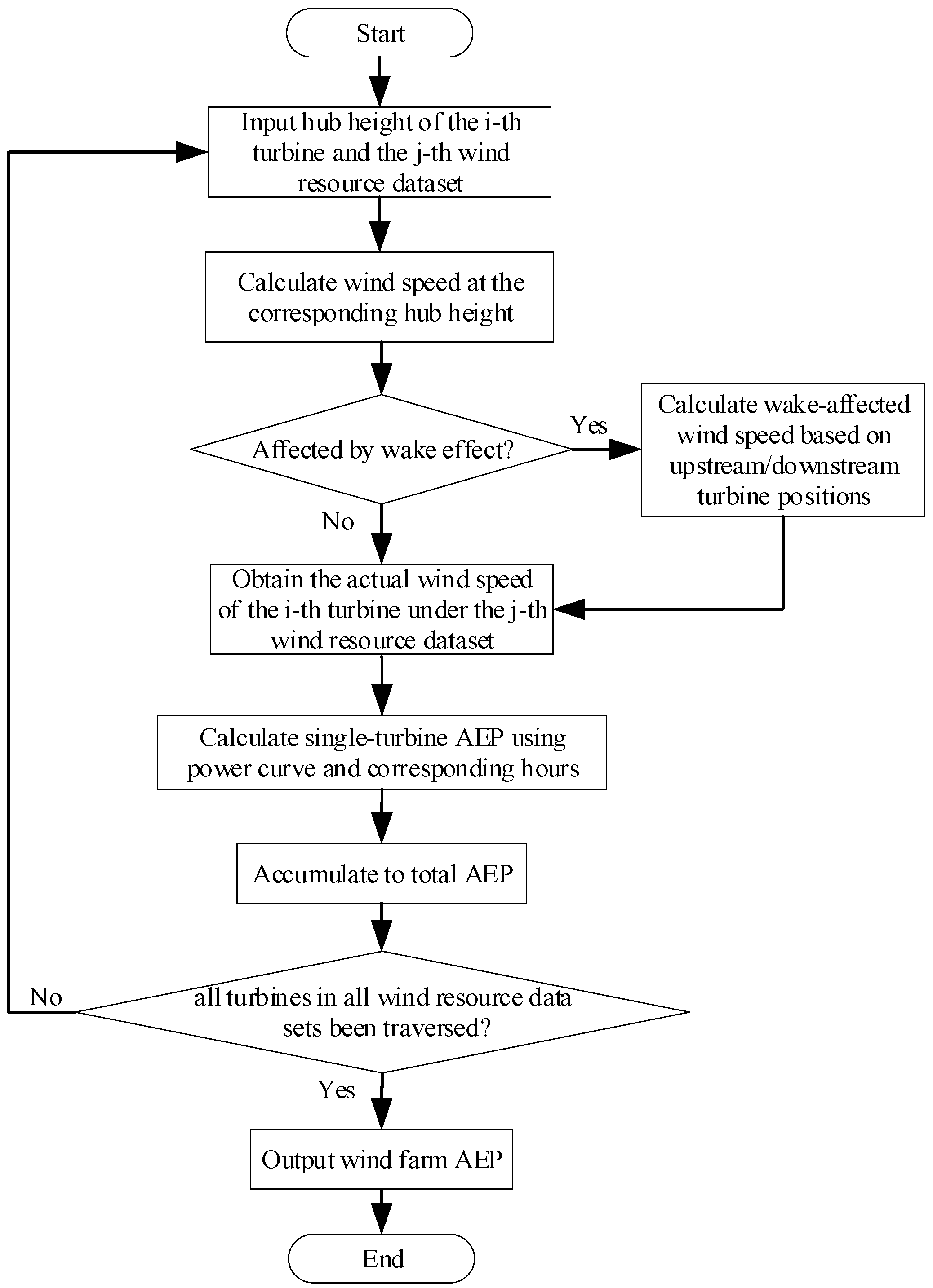
The above procedure is shown in Figure 4.

3. Formulation of the Optimization Model

To address the trade-off among wind directions in wind farm micro-siting when the optimization objective is the annual energy production across all wind directions, this paper proposes a wind farm layout strategy that combines horizontal and vertical staggering, with the objective of maximizing the simplified capital efficiency under the primary and secondary wind directions.

3.1. Selection of Primary and Secondary Wind Directions

To determine the primary and secondary wind directions at a given site, both wind energy and occurrence hours of each directional sector are evaluated based on the wind rose. The wind energy is calculated as follows:

$$W={\displaystyle \frac{1}{2}}\rho A{u}^3$$

(11)

where $W$ denotes the wind energy; $A$ is the cross-sectional area of the airflow; and $\rho$ is the air density.

Wind energy is proportional to the cube of wind speed, and in wind farm micro-siting, the direction with the highest wind energy is typically defined as the primary wind direction. Therefore, the sum of the cube of wind speed for each directional sector is calculated, and the primary wind direction is determined by identifying the sector with the maximum value. Take a 16-sector wind direction division as an example:

$$\max \left\{\left.{\displaystyle {\displaystyle \sum _{i=1}^{m_1}}{u}_{1i}^3{h}_{1i}},\cdots ,{\displaystyle {\displaystyle \sum _{i=1}^{m_{16}}}{u}_{16i}^3{h}_{16i}}\right\}\right.$$

(12)

where $m_1,\cdots ,m_{16}$ denotes the number of wind speed bins in each directional sector; $u_{1i},\cdots ,u_{16i}$ represents the wind speed values corresponding to each sector; and $h_{1i},\cdots ,h_{16i}$ is the total number of hours associated with each wind speed within the sector. The secondary wind direction is determined in the same manner.

3.2. Combination of Horizontal and Vertical Staggering

Horizontal staggering refers to introducing a lateral offset between upstream and downstream turbines in the direction perpendicular to the primary wind direction. Its physical basis lies in exploiting the lateral expansion of the wake, allowing downstream turbines to avoid the wake core region of upstream turbines. In contrast, vertical staggering is achieved by adjusting turbine hub heights to create a vertical separation between upstream and downstream turbines. The advantages of vertical staggering are twofold. First, by utilizing the vertical wind speed profile, downstream turbines can operate in regions with higher wind speeds, partially compensating for wake-induced velocity deficits. Second, the height difference enables downstream turbines to avoid the core deficit region of the upstream wake, yielding an effect similar to horizontal staggering. Therefore, combining horizontal and vertical staggering is expected to achieve greater overall benefits.

In Section 3.1, the primary and secondary wind directions were identified based on statistical data of local wind speed and wind direction. In terms of layout strategy, turbines are first arranged using horizontal staggering along the secondary wind direction, following conventional empirical layout approaches. According to common engineering practice, the spacing between turbines in the primary wind direction is typically no less than three rotor diameters, while the spacing in the direction perpendicular to the primary wind direction is no less than five rotor diameters. While this configuration effectively reduces wake effects and enhances power generation efficiency, the conservative spacing leads to a dispersed layout and limited site utilization.

To address this limitation, the turbine spacing in the horizontal staggering layout is reduced to three and two rotor diameters along the secondary wind direction and its perpendicular direction, respectively. Let $\left(X_i,Y_i\right)$ denote the coordinates of the wind turbines, then the following constraints must be satisfied:

$$\left\{\begin{array}{l}0\le X_i\le l_1\\ 0\le Y_i\le l_2\end{array}\right.,i=1,2,\cdots ,N$$

(13)

where $l_1$ and $l_2$ denote the length and width of the wind farm respectively. This constraint ensures that all turbines are located within the wind farm boundary. Based on this initial layout, THRO algorithm is further introduced to optimize the hub heights of individual turbines. The horizontal coordinates of all turbines are predetermined by the staggered layout described in this section. THRO is subsequently applied to optimize the hub-height assignment for each turbine position. By appropriately selecting hub heights with respect to the primary and secondary wind directions in the vertical dimension, the proposed approach enhances spatial compactness and capital efficiency while maintaining power generation efficiency.

3.3. Objective Function and Constraints

This study considers both turbine construction cost and annual energy production, and defines the objective function as the maximization of simplified capital efficiency (power generation per unit capital cost) under primary and secondary wind direction conditions. The cost term in this objective function includes only turbine base cost and tower cost, which are the cost components directly affected by hub-height selection. This simplified capital efficiency, this simplified metric serves as a capital-efficiency indicator rather than a full economic performance measure, as expressed below:

$$\max F={\displaystyle \frac{AE{P}_{main}+AE{P}_{second}}{C_{total}}}$$

(14)

where $AE{P}_{main}$ denotes the total annual energy production of the wind farm under the primary wind direction; $AE{P}_{second}$ denotes the total annual energy production under the secondary wind direction; and $C_{total}$ represents the total construction cost of the wind farm, which consists of two components: the turbine foundation cost and the tower cost per unit height:

$$C_{total}=C_{tower,base}\cdot N+C_{per,metre}\cdot {\displaystyle \sum _{i=1}^N{h}_i}$$

(15)

where $C_{tower,base}$ denotes the base construction cost of a single wind turbine; and $C_{per,metre}$ represents the tower cost per unit height; $h_i$ denote the hub height corresponding to the i-th wind turbine, this simplified cost metric excludes foundation costs, installation, array cables, substations, operation and maintenance, and other life-cycle costs.

Since the horizontal turbine coordinates are fixed by the initial staggered layout and are not modified during the THRO optimization process, the minimum spacing constraint is guaranteed at the layout generation stage. Specifically, during the construction of the initial staggered layout described in Section 3.2, the spacing between any two adjacent turbines is set to no less than 2D in the along-wind direction and no less than 3D in the cross-wind direction, where D is the rotor diameter. This ensures that all candidate layouts evaluated during the optimization process inherently satisfy the minimum spacing requirement without the need for additional constraint enforcement.

4. Tian Ji’s Horse Racing Optimization Algorithm

4.1. Algorithm Inspiration and Basic Principles

The Tian Ji’s Horse Racing Optimization (THRO) algorithm is a novel metaheuristic algorithm proposed by Wang et al. in 2025 [24], inspired by the ancient Chinese game strategy of “Tian Ji’s Horse Racing.” The story of Tian Ji’s horse racing dates back to the Spring and Autumn and Warring States periods. Tian Ji and the King of Qi each possessed three classes of horses: upper, middle, and lower. In each class, the King’s horse was slightly faster than Tian Ji’s corresponding horse. Under the conventional pairing (upper versus upper, middle versus middle, lower versus lower), Tian Ji lost all three races. Tian Ji’s military adviser then proposed the following strategy: in the first race, match the lower-class horse against the King’s upper-class horse (a deliberate loss to exhaust the opponent’s strongest horse); in the second race, match the upper-class horse against the King’s middle-class horse (securing a win); and in the third race, match the middle-class horse against the King’s lower-class horse (securing another win). Ultimately, Tian Ji won with a score of 2:1.

This story reveals a core idea in game theory: “use the weak to counter the strong, use the strong to counter the medium, and use the medium to counter the weak”—by dynamically matching with appropriate opponents, the overall payoff is maximized rather than pursuing a local victory in each individual round. The THRO generalizes this idea into a dual-population co-evolutionary optimization algorithm. The algorithm maintains two populations:

Tian Ji population: ${\mathit{X}}_T={\left[{\mathit{x}}_{T1},{\mathit{x}}_{T2}\mathbf{,}\cdots \mathbf{,}{\mathit{x}}_{Tn}\right]}^T$.

Qi Wang population: ${\mathit{X}}_K={\left[{\mathit{x}}_{K1},{\mathit{x}}_{K2}\mathbf{,}\cdots \mathbf{,}{\mathit{x}}_{Kn}\right]}^T$.

Each population consists of n individuals (corresponding to n horses), and each individual x represents a candidate solution, i.e., an encoding scheme for the wind turbine types within the wind farm, where the encoding takes a value of 0 or 1. 0 denotes a low-hub wind turbine and 1 denotes a high-hub wind turbine. In a minimization problem, a smaller fitness value of an individual indicates a faster running speed. Through competition and synergy between the two populations, the algorithm drives the individuals to approach the global optimal solution.

4.2. Competition Phase Based on Dynamic Individual Matching Strategy

The core innovation of the THRO lies in its “dynamic matching–competition” mechanism. At the beginning of each iteration, the two populations are separately sorted in ascending order of fitness values (the individual with the smallest fitness is the fastest and is ranked first). Subsequently, n rounds of “races” are conducted. In each round, one of five strategies is selected and executed based on the relative speed relationship between the slowest and the fastest individuals among the remaining horses.

Let ${\mathit{x}}_T^{slow}$ and ${\mathit{x}}_K^{slow}$ denote the current slowest individuals of the Tian Ji population and the Qi Wang population, respectively; ${\mathit{x}}_T^{fast}$ and ${\mathit{x}}_K^{fast}$ denote the current fastest individuals of the Tian Ji population and the Qi Wang population, respectively; $f\left(x\right)$ is the fitness function; The specific strategies are as follows:

Strategy 1: The slowest Tian Ji horse is faster than the slowest Qi Wang horse.

When $f\left({\mathit{x}}_T^{slow}\right)<f\left({\mathit{x}}_K^{slow}\right)$, the slowest Tian Ji horse is still faster than the slowest Qi Wang horse. In this case, Tian Ji uses a strong horse against a weak opponent, securing a win in this round.

Strategy 2: The slowest Tian Ji horse is slower than the slowest Qi Wang horse.

When $f\left({\mathit{x}}_T^{slow}\right)>f\left({\mathit{x}}_K^{slow}\right)$, the slowest Tian Ji horse is slower than the slowest Qi Wang horse. In this case, Tian Ji uses the weakest horse to consume the strongest horse of the Qi Wang population, conceding defeat in this round.

Strategy 3: The slowest horses are equal, and the fastest Tian Ji horse is faster than the fastest Qi Wang horse.

When $f\left({\mathit{x}}_T^{slow}\right)=f\left({\mathit{x}}_K^{slow}\right)$ and $f\left({\mathit{x}}_T^{fast}\right)<f\left({\mathit{x}}_K^{fast}\right)$ hold, Tian Ji adopted a “strong against strong” strategy, using his fastest horse to race against King Qi’s fastest horse and won.

Strategy 4: The slowest horses are equal, and the fastest Tian Ji horse is slower than the fastest Qi Wang horse.

When $f\left({\mathit{x}}_T^{slow}\right)=f\left({\mathit{x}}_K^{slow}\right)$ and $f\left({\mathit{x}}_T^{fast}\right)>f\left({\mathit{x}}_K^{fast}\right)$ hold, Tian Ji is unable to secure a win in the fastest-horse matchup; therefore, it adopts the “weak versus strong” approach from Strategy 2, using the slowest horse to consume the fastest horse of the Qi Wang population.

Strategy 5: The slowest horses are equal, and the fastest horses are also equal.

When $f\left({\mathit{x}}_T^{slow}\right)=f\left({\mathit{x}}_K^{slow}\right)$ and $f\left({\mathit{x}}_T^{fast}\right)=f\left({\mathit{x}}_K^{fast}\right)$ hold, the strengths of both sides are completely matched. Tian Ji still adopts the “weak versus strong” strategy.

The detailed update equations for all five strategies, including the Lévy flight step generation, are provided in Appendix A.

4.3. Training Phase with Differential Mutation and Elite Guidance

After completing the n rounds of competition, the algorithm proceeds to the training phase, in which each individual in both populations undergoes auxiliary updates to further exploit local information around high-quality solutions. The training phase comprises two modes, selected by a random threshold $rand\in [0,1]$:

Mode 1: Differential mutation strategy. When $rand>0.5$ is satisfied, differential mutation is employed to generate candidate individuals.

Mode 2: Elite guidance strategy. When $rand\le 0.5$ is satisfied, candidate individuals move towards the current optimal individual of the population.

After the training phase is completed, the fitness of the newly generated candidate individuals is evaluated, and they replace the original individuals if they are superior. This phase further enhances the local exploitation capability of the algorithm based on the competition phase, while the differential mutation mode preserves the possibility of escaping from local optima.

The complete training phase formulations are provided in Appendix A.

4.4. THRO Algorithm Procedure

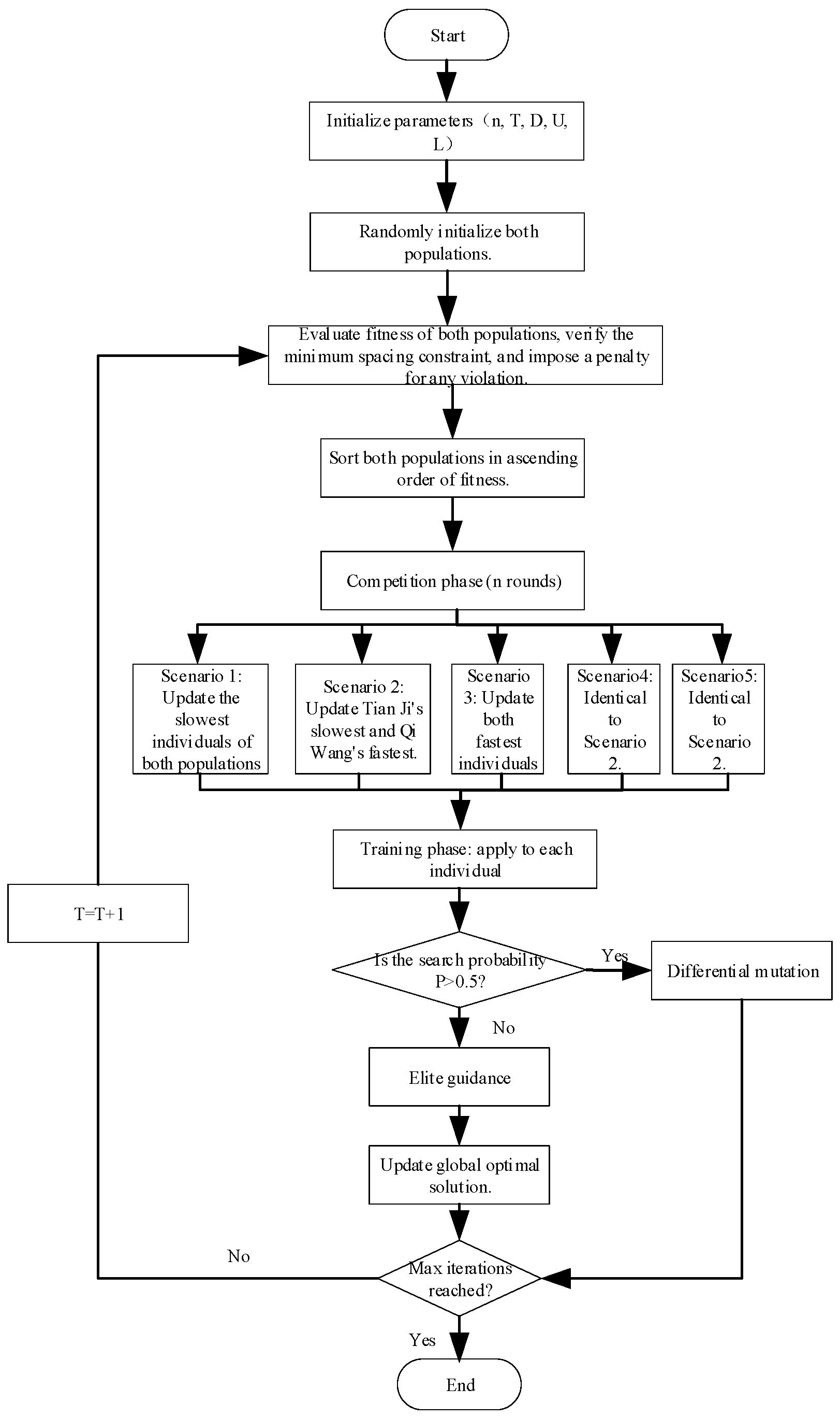
In the implementation of offshore wind farm micro-siting, the specific steps of applying the THRO algorithm are as follows:

Step 1: Initialize the parameters, including the population size n (representing different layout schemes), the maximum number of iterations T, the variable dimension D, and the upper and lower bounds U and L of the variables.

Step 2: Randomly initialize the Tian Ji population ${\mathit{X}}_T$ and the Qi Wang population ${\mathit{X}}_K$:

$$x_{i,j}=L_j+\mathrm{rand}\cdot (U_j-L_j),\hspace{1em}i=1,2,\dots ,n;\hspace{1em}j=1,2,\dots ,D$$

(16)

Since the THRO algorithm operates in the continuous domain while the actual turbine hub-height assignment requires binary decisions (0 for low hub, 1 for high hub), a discretization mechanism is applied after each update:

(1) Boundary clamping: All continuous values $x_{i,j}$ are first clipped to the feasible range [0,1]. If $x_{i,j}<0$ it is set to 0; If $x_{i,j}>1$, it is set to 0.

(2) Stochastic thresholding: Before fitness evaluation, each clamped continuous value $x_{i,j}$ is converted into a binary decision $b_i\in \{0,1\}$ using a random threshold: $b_i=1$ if $x_i>rand(0,1)$, otherwise $b_i=0$. This stochastic mapping preserves the exploration capability of the algorithm while ensuring that all evaluated layouts are physically feasible binary configurations.

Step 3: Sort the two populations separately in ascending order of fitness values (a smaller fitness value indicates a better individual).

Step 4: For each individual in both populations, repeat the following process:

(1) Identify the current slowest individual ${\mathit{x}}_T^{slow}$ and the fastest individual ${\mathit{x}}_T^{fast}$ in the Tian Ji population;

(2) Identify the current slowest individual ${\mathit{x}}_K^{slow}$ and the fastest individual ${\mathit{x}}_K^{fast}$ in the Qi Wang population;

(3) According to the five strategy conditions described in Section 3.2, select the corresponding strategy to update the individual;

(4) Update the index pointers of the slowest and fastest individuals (matched individuals are removed from subsequent races);

(5) Evaluate the fitness of the new individuals, also subjecting them to constraint checking and penalization according to Equation (16), and replace the original individuals if the new ones are superior.

Step 5: For each individual in both populations, generate a candidate new individual according to one of the two modes described in Section 3.3. The fitness of the candidate individual is then evaluated, and it replaces the original individual if it is superior.

Step 6: Identify the individual ${\mathit{x}}_{best}$ with the minimum fitness value from the two populations, and update the global optimal solution and the corresponding global optimal fitness value $f_{best}$.

Step 7: If the current number of iterations t < T, set t = t + 1 and proceed to Step 3; otherwise, output the global optimal solution ${\mathit{x}}_{best}$.

The complete flowchart of the algorithm is shown in Figure 5.

5. Case Study

5.1. Description of Offshore Wind Farms

This study considers an offshore site located in Shanghai. The wind farm is assumed to have a rectangular shape with a length of 4 km and a width of 3 km. A total of 71 wind turbines, each rated at 6 MW, are considered in this case study. The relevant basic parameters of the wind turbine are listed in

Table 1. Basic parameters of the wind turbine.

Parameters	Value
Rated Power/kW	6000
Rotor Radius/m	77
Hub Height/m	103.5/163.5
Cut-in Wind Speed/(m/s)	3
Rated Wind Speed/(m/s)	12
Cut-out Wind Speed/(m/s)	25

Note: Vertical staggering is represented solely by differences in turbine hub height.

.

The cost parameters of the wind turbine are listed in

Table 2. Cost parameters of the wind turbine.

Cost Category	Value
Base Cost/104 CNY	481
Tower Cost/(104 CNY/m)	3.64

.

The 8760 h of wind speed and direction data used in this study were collected at 10 m height from a measurement station located in the nearshore waters of Shanghai. The dataset contains over 8300 valid records, covering more than 95% of the annual period. Data preprocessing included the following steps: (1) outlier removal—records with negative wind speeds or values outside the physically reasonable range (0–40 m/s) were discarded; (2) missing data treatment—gaps of no more than 3 consecutive hours were filled using linear interpolation, while longer gaps were excluded without imputation; and (3) calm wind treatment—records with zero wind speed and zero wind direction were retained as calm conditions. The air density was assumed to be 1.225 kg/m³, corresponding to standard atmospheric pressure and 15 °C at sea level.

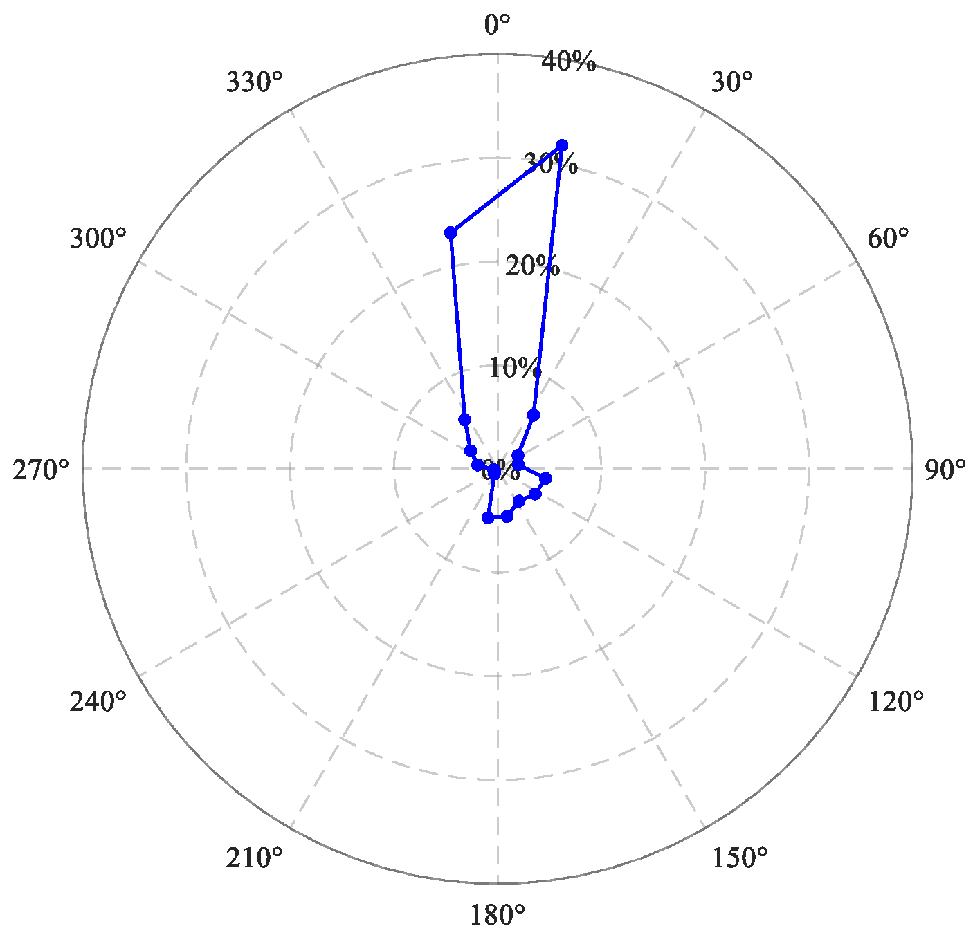
The 8760 h of measured wind speed and wind direction data at 10 m height are used to compute the wind energy share of each directional sector according to Equation (12), and a wind energy rose diagram is obtained, as shown in Figure 6. As shown in Figure 6, the site exhibits a primary wind direction and a secondary wind direction (${22.5}^{\circ }$, ${337.5}^{\circ }$) with a small angular difference, corresponding to wind energy shares of 31.79% and 23.22%, respectively, and the combined proportion of the primary and secondary wind directions exceeds 50%.

5.2. Optimization Results

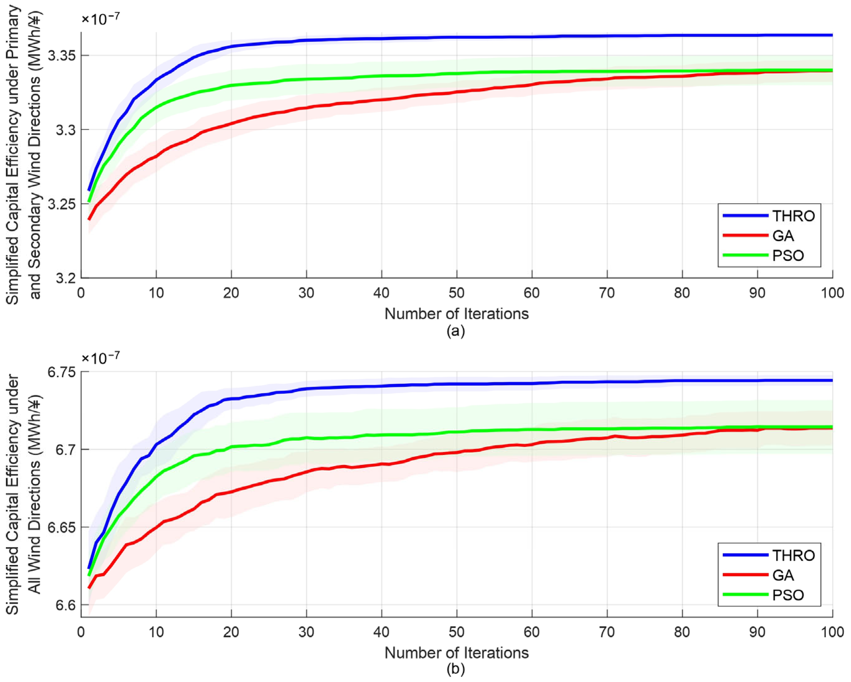
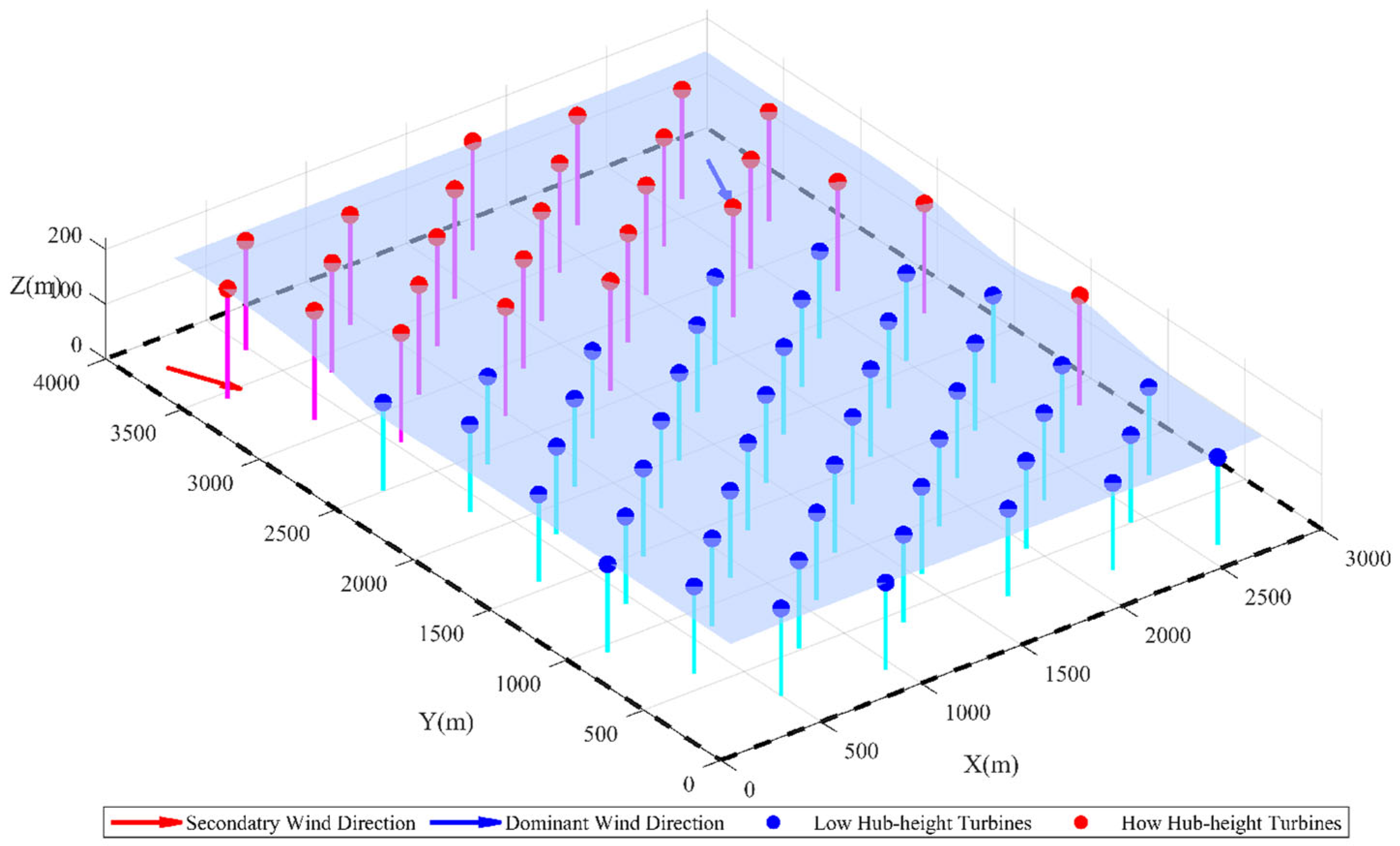
To ensure that the minimum fitness value is achieved, the negative reciprocal of the simplified capital efficiency in the primary and secondary wind direction is adopted as the fitness function. The initial population size is set to 80, and the maximum number of iterations is set to 100. The Tian Ji’s Horse Racing Optimization (THRO) algorithm is employed for iterative computation. To verify that this objective function does not compromise the simplified capital efficiency across all wind directions, the iteration curves record both the simplified capital efficiency under the primary and secondary wind directions and that under all wind directions. Comparisons are also made with the GA and PSO algorithms. The comparative iteration curves and the layout distribution based on the THRO algorithm are shown in Figure 7 and Figure 8, respectively. To quantitatively evaluate the statistical performance, all three algorithms were independently run 30 times under identical conditions.

Table 3. (a). Statistical comparison of THRO, GA, and PSO over 30 independent runs—AEP and power generation performance. (b). Statistical comparison of THRO, GA, and PSO over 30 independent runs—convergence and computational cost.

(a)
Algorithm	Best (MWh/¥) × 10−7	Worst (MWh/¥) × 10−7	Mean (MWh/¥) × 10−7	Std. Dev. × 10−10
THRO	3.365	3.359	3.363	1.931
GA	3.354	3.322	3.339	7.397
PSO	3.357	3.323	3.340	10.066
(b)
Algorithm	Avg. Converg. Iter.		Avg. Time (s)
THRO	39		285.53
GA	85		878.67
PSO	65		468.60

a,b summarize the statistical results over the 30 runs, including the best, worst, mean, and standard deviation of the simplified capital efficiency (Table 3a), as well as the average convergence iterations and average computational time (Table 3b).

To statistically evaluate the optimization performance, all algorithms were independently run 30 times under identical stopping criteria and computational budgets. Figure 7 presents the convergence trajectories of THRO, GA, and PSO for the subproblem of hub-height optimization with a fixed horizontal layout, where solid lines denote the mean simplified capital efficiency and shaded bands represent the range of variation across the 30 runs. As shown in Figure 7, THRO converges on average within 39 iterations, substantially faster than GA (approx. 85 iterations) and PSO (approx. 65 iterations). The mean simplified capital efficiency achieved by THRO is 3.365 × 10⁻⁷ MWh/Yuan under the primary and secondary wind directions and 6.746 × 10⁻⁷ MWh/Yuan under all-direction evaluation. This indicates that in scenarios where the wind energy share of the primary and secondary wind directions is relatively large, the improvement in the simplified capital efficiency under the primary and secondary wind directions simultaneously enhances the simplified capital efficiency under the full wind direction scenario. The shaded bands further reveal that THRO exhibits the narrowest convergence variability among the three algorithms, confirming its stable search performance.

The statistical results over the 30 independent runs are further summarized in Table 3a,b. Table 3a reports the best, worst, mean, and standard deviation of the simplified capital efficiency, while Table 3b presents the average convergence iterations and average computational time for each algorithm. As shown in Table 3a, THRO achieves the highest mean simplified capital efficiency (3.359 × 10⁻⁷ MWh/¥) with the smallest standard deviation (1.931 × 10⁻¹⁰), confirming its superior optimization accuracy and robustness. Table 3b further shows that THRO converges on average within 39 iterations with a computational time of 118 s per run, which is substantially faster than GA (85 iterations, 878 s) and PSO (65 iterations, 468 s). These statistical results demonstrate that THRO consistently outperforms GA and PSO across multiple runs, verifying its statistical superiority and reliable convergence behavior.

To provide a direct comparison with conventional all-direction optimization, we performed an additional optimization run using the full-direction efficiency as the objective function, under identical conditions (same site, same turbine count, same algorithm parameters). The results show that the full-direction efficiency obtained by our proposed primary + secondary optimization is 6.746 × 10⁻⁷ MWh/¥, while the full-direction optimization yields 6.664 × 10⁻⁷ MWh/¥, representing an improvement of approximately 1.23%. This confirms that prioritizing the primary and secondary wind directions does not compromise the full-direction performance; rather, it enhances it by more effectively capturing wind energy in the dominant sectors.

Further analysis of Figure 8 allows the following layout patterns to be summarized:

(1) When both the primary and secondary wind directions are considered, the optimal layout tends to place high-hub wind turbines in the windward direction of the wind farm, i.e., in the front rows on the inflow side of the primary and secondary wind directions, in order to reduce the impact of the wake effect on downstream turbines. According to the wind shear calculation formula, higher hub heights experience higher wind speeds, allowing high-hub turbines to more fully utilize the wind resource and improve the power generation efficiency per unit cost.

(2) Behind the front-row turbines, a large number of low-hub wind turbines are deployed. This serves two purposes: first, the low-hub turbines and the high-hub turbines in the front rows form a vertically staggered layout, complementing the pattern described in (1).

(3) The remaining turbines in the wind farm, being located downstream of the inflow direction, are severely affected by the cumulative wake effect from multiple front-row turbines. Although using high-hub turbines in this zone could increase power generation, the resulting benefits cannot compensate for the increased investment cost; therefore, low-hub turbines should be adopted.

5.3. Comparative Analysis with Other Approaches

In this section, the proposed THRO-based layout strategy is compared with two alternative horizontal layouts: a GA-PSO-optimized horizontal layout and a manual empirical layout. For these two reference layouts, all turbines are fixed at the low hub height (103.5 m) to isolate and evaluate the effectiveness of the horizontal staggering strategy. In contrast, the proposed THRO-based layout integrates both horizontal staggering (guided by the primary and secondary wind directions) and hub-height optimization. This comparison serves to demonstrate the combined benefits of the horizontal and vertical optimization approach. It should be noted that this comparison is distinct from that presented in Figure 7, where the focus is on algorithm-level performance for hub-height optimization with a fixed horizontal layout.

5.3.1. Manual Layout Method

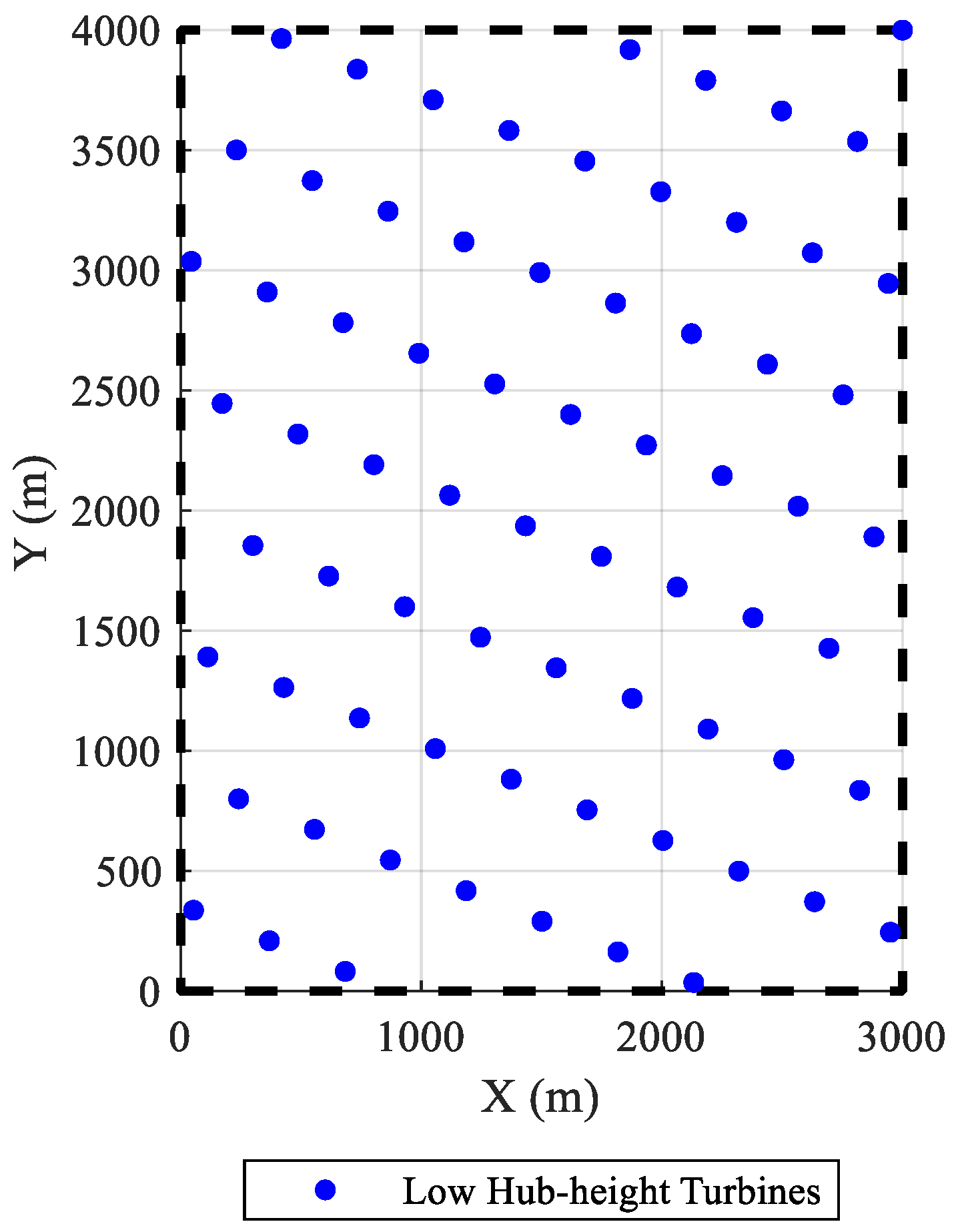
The manual layout method is used to arrange the wind turbines in the same offshore wind farm area. The specific rules are as follows: the turbines are placed in rows along the primary wind direction, with no horizontal offset between adjacent rows. The spacing between turbines is set to 2 times and 3 times the rotor diameter along the primary wind direction and the direction perpendicular to the primary wind direction, respectively. The resulting layout is shown in Figure 9.

Under this layout method, the annual power generation of the offshore wind farm is 426.82 GWh, while that in Section 4.2 is 449.14 GWh, representing an increase in power generation efficiency of approximately 5.23%.

5.3.2. GA-PSO Algorithm

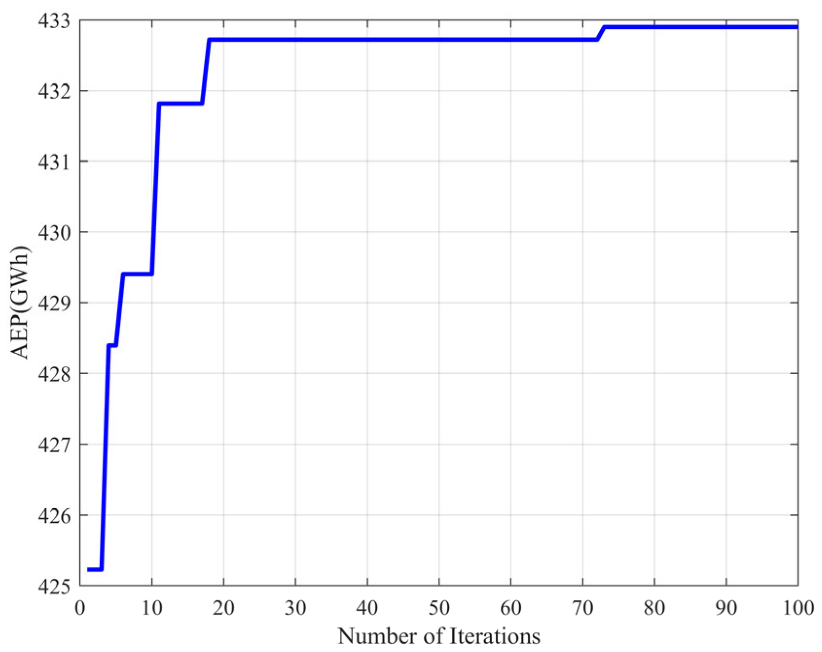
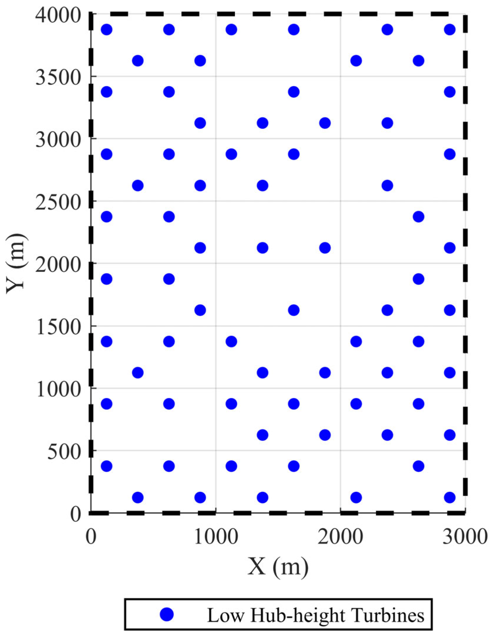
The wind farm is divided into squares with a side length of 250 m, each square representing a possible placement location. The initial population size is set to 80, and the maximum number of iterations is set to 100. The GA-PSO hybrid algorithm is employed for iterative computation, and the iteration curves and layout distribution are shown in Figure 10 and Figure 11, respectively.

Under this algorithm, the annual power generation of the offshore wind farm is 432.89 GWh, while that in Section 4.2 is 449.14 GWh, representing an increase in power generation efficiency of approximately 3.75%.

The comparison of the results obtained by the three methods is shown in

Table 4. Comparison of the results of the three algorithms.

Method	All-Dir AEP/GWh	Primary AEP/GWh	Secondary AEP/GWh	Convergence Iterations	High-Hub	Low-Hub
THRO algorithm	449.14	121.55	105.93	39	19	52
Manual layout Method	426.82	119.44	104.33	-	0	71
GA-PSO Algorithm	432.89	120.83	104.46	73	0	71

Note: “-” indicates that no intelligent algorithm is used.

.

The comparison in Table 4 focuses on energy production metrics to evaluate the effectiveness of the horizontal staggering strategy. In terms of turbine configuration, the THRO-based layout uses 19 high-hub turbines and 52 low-hub turbines, whereas the GA-PSO and manual layouts use only low-hub turbines (71 in total). Consequently, the total construction cost of THRO (650.49 M¥) is higher than that of GA-PSO and the manual layout (608.99 M¥ for both), as the use of high-hub turbines increases tower costs. However, this additional investment yields a notable increase in annual energy production: THRO achieves 449.14 GWh, outperforming GA-PSO by 3.75% and the manual layout by 5.23%. The primary-direction AEP also shows consistent improvement. This confirms that the proposed horizontal staggering strategy, combined with appropriate hub-height allocation, effectively enhances energy production and justifies the additional cost.

6. Conclusions

This paper proposes a wind turbine layout strategy that combines horizontal and vertical staggering, and introduces the THRO algorithm to iteratively optimize the simplified capital efficiency under the primary and secondary wind directions, ultimately obtaining the optimal layout. The case study analysis shows that:

(1) Compared with the manual layout method that only considers the primary wind direction, the proposed method, which simultaneously considers both the primary and secondary wind directions, can more comprehensively account for the impact of wind direction variations on the power generation efficiency of the wind farm and make fuller use of the wind resource.

(2) On the basis of determining the primary and secondary wind directions, combining vertical staggering with horizontal staggering can effectively mitigate the impact of the wake effect and increase the power generation per unit cost.

(3) The THRO algorithm is capable of escaping the local minimum. Compared with other algorithms, it converges more quickly, and the obtained optimal solution outperforms the comparative algorithms in terms of both convergence speed and solution quality. We acknowledge that the current study is based on a single offshore site, and the generalizability of the findings to other sites remains to be investigated. In addition, the optimization is limited to two discrete hub heights, while continuous or multi-height optimization may yield further improvements. Our cost model is also simplified, excluding foundation costs, installation, array cables, substations, operation and maintenance, availability, electrical losses, and financing.

In future research, the wake model can be further refined to incorporate atmospheric stability and turbulence intensity effects, which may influence wake recovery rates in offshore environments. Additionally, multiple wind turbines with different power ratings can be compared to screen out the optimal combination scheme, and different hub heights can be assigned to the same type of turbine to examine the impact of height variation on the simplified capital efficiency. A full life-cycle cost model (LCOE) incorporating the above-mentioned cost components will also be developed to provide a more comprehensive economic assessment, while future work may also incorporate reliability, as well as economic and environmental factors.

References

1. Cabo-Rodríguez, A.; Calvo-Silvosa, A.; DeLlano-Paz, F. Economic Valuation under Uncertainty in Offshore Wind Farms Investments: A Systematic Literature Review. Appl. Energy 2026, 409, 127520. [Google Scholar] [CrossRef] [Scilit]
2. Schulz, C.W.; Bergua, R.; Branlard, E.; Netzband, S.; Jonkman, J.; Roberston, A. Unsteady Aerodynamics of Large-Scale Floating Offshore Wind Turbines in Surge Motion. Renew. Energy 2026, 260, 124977. [Google Scholar] [CrossRef] [Scilit]
3. Mosetti, G.; Poloni, C.; Diviacco, B. Optimization of Wind Turbine Positioning in Large Windfarms by Means of a Genetic Algorithm. J. Wind Eng. Ind. Aerodyn. 1994, 51, 105–116. [Google Scholar] [CrossRef] [Scilit]
4. Liu, Y. The Effect of Vertical Arrangement on Performance and Wake Characteristics of Two Tandem Offshore Wind Turbines under Various Operating Conditions. Energy Convers. Manag. 2023, 278, 116743. [Google Scholar] [CrossRef] [Scilit]
5. Herbert-Acero, J.-F.; Franco-Acevedo, J.-R.; Valenzuela-Rendon, M.; Probst-Oleszewski, O. Linear Wind Farm Layout Optimization through Computational Intelligence. In Proceedings of the MICAI 2009: Advances in Artificial Intelligence, Proceedings; Aguirre, A.H., Borja, R.M., Garcia, C.A.R., Eds.; Springer: Guanajuato, Mexico, 2009; Volume 5845, pp. 692–703. [Google Scholar]
6. Chen, Y.; Li, H.; Jin, K.; Song, Q. Wind Farm Layout Optimization Using Genetic Algorithm with Different Hub Height Wind Turbines. Energy Convers. Manag. 2013, 70, 56–65. [Google Scholar] [CrossRef] [Scilit]
7. Archer, C.L.; Vasel-Be-Hagh, A.; Yan, C.; Wu, S.; Pan, Y.; Brodie, J.F.; Maguire, A.E. Review and Evaluation of Wake Loss Models for Wind Energy Applications. Appl. Energy 2018, 226, 1187–1207. [Google Scholar] [CrossRef] [Scilit]
8. Tao, S.; Kuenzel, S.; Xu, Q.; Chen, Z. Optimal Micro-Siting of Wind Turbines in an Offshore Wind Farm Using Frandsen–Gaussian Wake Model. IEEE Trans. Power Syst. 2019, 34, 4944–4954. [Google Scholar] [CrossRef] [Scilit]
9. Miao, D.; Liu, Q.; Li, H.; Yin, W.; Zhou, C. Analysis of Wake Model Characteristics Based on Wind Field Experiments and Numerical Simulations. J. Wind Eng. Ind. Aerodyn. 2026, 271, 106374. [Google Scholar] [CrossRef] [Scilit]
10. Shid-Moosavi, S.; Di Cioccio, F.; Haghi, R.; Tronci, E.M.; Moaveni, B.; Liberatore, S.; Hines, E. Modeling and Experimentally-Driven Sensitivity Analysis of Wake-Induced Power Loss in Offshore Wind Farms: Insights from Block Island Wind Farm. Renew. Energy 2025, 241, 122126. [Google Scholar] [CrossRef] [Scilit]
11. Orlova, S.; Dmitrijevs, N.; Mironova, M.; Komasilovs, V.; Kamolins, E. Assessment of Onshore and Offshore Wind Energy Potential in the Eastern Baltic Sea Region: LCOE and Wind Turbine Layout Optimisation. Energies 2026, 19, 1448. [Google Scholar] [CrossRef] [Scilit]
12. Feng, J.; Shen, W.Z. Modelling Wind for Wind Farm Layout Optimization Using Joint Distribution of Wind Speed and Wind Direction. Energies 2015, 8, 3075–3092. [Google Scholar] [CrossRef] [Scilit]
13. Lu, Y.; Matheou, G. Wind Direction Effects on Power Production of the South Fork Offshore Wind Farm. In Proceedings of the 57th North American Power Symposium, NAPS 2025, Hartford, CT, USA, 26–28 October 2025; Institute of Electrical and Electronics Engineers Inc.: Storrs, CT, USA, 2025. [Google Scholar]
14. Song, M.; Chen, K.; Zhang, X.; Wang, J. Optimization of Wind Turbine Micro-Siting for Reducing the Sensitivity of Power Generation to Wind Direction. Renew. Energy 2016, 85, 57–65. [Google Scholar] [CrossRef] [Scilit]
15. Archer, C.L.; Mirzaeisefat, S.; Lee, S. Quantifying the Sensitivity of Wind Farm Performance to Array Layout Options Using Large-Eddy Simulation. Geophys. Res. Lett. 2013, 40, 4963–4970. [Google Scholar] [CrossRef] [Scilit]
16. Yang, S.; Deng, X.; Yang, K. Machine-Learning-Based Wind Farm Optimization through Layout Design and Yaw Control. Renew. Energy 2024, 224, 120161. [Google Scholar] [CrossRef] [Scilit]
17. He, J.; Ge, M.; Žarković, S.D.; Li, Z.; Hilber, P. A Novel Integrated Optimization Method of Micrositing and Cable Routing for Offshore Wind Farms. Energy 2024, 306, 132443. [Google Scholar] [CrossRef] [Scilit]
18. Tang, X.-Y.; Yang, Q.; Stoevesandt, B.; Sun, Y. Optimization of Wind Farm Layout with Optimum Coordination of Turbine Cooperations. Comput. Ind. Eng. 2022, 164, 107880. [Google Scholar] [CrossRef] [Scilit]
19. Lu, B.; Shen, X.; Du, Y.; Huang, Z.; Tan, R. Offshore Wind Farm Micro-Siting Based on Two-Phase Hybrid Optimization. Appl. Energy 2025, 381, 125105. [Google Scholar] [CrossRef] [Scilit]
20. Yin, P.-Y.; Wu, T.-H.; Hsu, P.-Y. Risk Management of Wind Farm Micro-Siting Using an Enhanced Genetic Algorithm with Simulation Optimization. Renew. Energy 2017, 107, 508–521. [Google Scholar] [CrossRef] [Scilit]
21. Huang, Z.; Yuan, C.; Ge, H.; Hou, T. Optimization of Substation Siting and Connection Topology in Offshore Wind Farm Based on Modified Firefly Algorithm. IEEE J. Emerg. Sel. Top. Circuits Syst. 2023, 13, 806–816. [Google Scholar] [CrossRef] [Scilit]
22. Chen, K.; Song, M.X.; Zhang, X.; Wang, S.F. Wind Turbine Layout Optimization with Multiple Hub Height Wind Turbines Using Greedy Algorithm. Renew. Energy 2016, 96, 676–686. [Google Scholar] [CrossRef] [Scilit]
23. Shaban, A.; Al-Hinai, N.; Abdelhady, S. A Novel Simulation–Optimization Framework for Techno-Economic Analysis and Optimal Design of Wind Energy Systems with NPV Maximization. Energy Convers. Manag. X 2026, 30, 101643. [Google Scholar] [CrossRef] [Scilit]
24. Wang, L.; Du, H.; Zhang, Z.; Hu, G.; Mirjalili, S.; Khodadadi, N.; Hussien, A.G.; Liao, Y.; Zhao, W. Tianji’s Horse Racing Optimization (THRO): A New Metaheuristic Inspired by Ancient Wisdom and Its Engineering Optimization Applications. Artif. Intell. Rev. 2025, 58, 282. [Google Scholar] [CrossRef] [Scilit]
Figure 1. Offshore wind farm.
Energies 19 03955 g001
Figure 2. Schematic diagram of wake effects.
Energies 19 03955 g002
Figure 3. Schematic diagram of partial wake overlap.
Energies 19 03955 g003
Figure 4. Flowchart of AEP calculation for a wind farm.
Energies 19 03955 g004
Figure 5. Flowchart of the Tian Ji’s Horse Racing Optimization (THRO) algorithm.
Energies 19 03955 g005
Figure 6. Wind rose diagram.
Energies 19 03955 g006
Figure 7. Convergence curves of simplified capital efficiency for THRO, GA, and PSO over 30 independent runs (solid lines: mean values; shaded bands: variation range across 30 runs). (a) Under primary and secondary wind directions; (b) under all wind directions.
Energies 19 03955 g007
Figure 8. Offshore wind farm layout optimized by the THRO algorithm.
Energies 19 03955 g008
Figure 9. Layout of the offshore wind farm using the manual layout method.
Energies 19 03955 g009
Figure 10. Iteration curve of annual power generation using the GA-PSO algorithm.
Energies 19 03955 g010
Figure 11. Layout of the offshore wind farm using the GA-PSO algorithm.
Energies 19 03955 g011