Multi-Year Assessment of the Real-World Performance of Residential Photovoltaic Microinstallations in the Sandomierz Basin, Southeastern Poland

Abstract

The rapid expansion of residential photovoltaics (PV) increases the need for long-term evidence on system performance under real operating conditions. This study compared four grid-connected rooftop PV microinstallations (4.69–5.04 kWp) located in the Sandomierz Basin, southeastern Poland, over 2022–2025. Monthly alternating-current production from SolarEdge monitoring was combined with regional sunshine duration and mean air temperature from the IMGW Sandomierz station, providing 192 installation–month observations. Specific yield, capacity factor, a model-based estimate of the performance ratio (PR_AP), Pearson correlations, ordinary least-squares regression, and sensitivity analysis of a documented failure were applied. Mean annual specific yields were 1077.7, 1061.7, 908.6, and 779.6 kWh/kWp for PV-I–PV-IV, respectively, while mean PR_AP estimates were 82.2%, 82.5%, 70.6%, and 65.5%. Sunshine duration was strongly correlated with monthly specific yield (r = 0.830–0.983; p < 0.001), and the combined model explained 88.8% of its variability. Excluding the zero-output failure month of PV-IV increased R² for the sunshine–yield relationship from 0.689 to 0.812 and improved the combined-model fit from 0.888 to 0.921. Greater nominal capacity did not guarantee higher normalized productivity. Regional solar-resource information should therefore be complemented by monitored operational data to support design, benchmarking, fault detection, and local distributed-energy planning. The findings also support SDG 7 by providing evidence for more reliable, locally adapted planning and operation of household photovoltaic systems.

1. Introduction

Photovoltaic systems have become one of the most important components of the global energy transition [1,2]. Their development is supported by climate policy, growing demand for low-emission energy sources, declining technology costs, efforts to enhance energy security, and the need to diversify electricity generation [3,4]. In recent years, photovoltaics has ceased to be a niche technology and has become one of the main directions for developing new generation capacity, both in large industrial installations and in distributed sources operating directly at end-user sites [5,6].

As deployment has expanded, not only installed capacity but also the actual productivity of PV systems under operating conditions has become increasingly important [7,8]. Energy production from real installations depends on a range of factors that are not always fully considered at the design stage. These include local solar-radiation availability, module temperature, panel orientation and tilt angle, shading, soiling, inverter characteristics, grid constraints, and system downtime [9,10,11,12,13]. For this reason, studies based on monitored data are becoming increasingly valuable because they make it possible to assess the actual behavior of installations over multiple years of operation [14]. Small rooftop and prosumer installations form a particularly important group because their technical configuration is often constrained by the existing building architecture [15,16,17]. Unlike large photovoltaic farms, where module orientation, tilt, and arrangement can be designed with energy optimization in mind, rooftop microinstallations are usually mounted on available roof surfaces [18,19,20]. In practice, systems with similar nominal capacities may achieve different energy yields when they operate at different azimuths, tilt angles, levels of local shading, or under other differing operating conditions [21,22,23,24]. This issue is important not only technically but also practically. From the perspective of the prosumer, designer, grid operator, and local authorities, nominal installation capacity alone is insufficient to evaluate performance [25,26]. It is also important to determine whether a given installation actually uses the available solar-radiation potential and which factors limit its productivity. Such an assessment is particularly important as the share of distributed energy sources increases, because the actual operating profiles of microinstallations affect self-consumption, local balancing, and distribution-grid loading [27,28].

In Poland, the rapid development of photovoltaic microinstallations has made the assessment of their actual yields important for both individual users and entities responsible for planning the local energy transition [25,26]. Prosumer installations are most often implemented on existing residential buildings; therefore, their orientation and tilt are more often determined by mounting conditions than by model-based production optimization [29,30,31,32,33]. Consequently, national and regional data on solar potential should be supplemented with analyses of actual installations operating under specific local conditions [7,8,34,35]. The literature on PV-system performance emphasizes that annual production expressed in kWh or MWh alone is not a sufficient measure of effectiveness [7,14]. Comparing installations with different capacities requires normalization of the results, most commonly by using specific yield, capacity factor, performance ratio, or other indicators relating actual energy production to system potential [36,37]. Specific yield is particularly useful for microinstallations because it allows systems with different nominal capacities to be compared and reduces the risk of the erroneous interpretation that greater installation capacity automatically means higher efficiency [10,11,12].

One of the key factors differentiating PV-system productivity is module orientation [18,22]. In the Northern Hemisphere, south-facing exposure usually favors maximum annual energy production; however, southeast-, southwest-, and west-facing configurations are also common in prosumer installations [19,20]. Such configurations may reduce total annual yield while changing the daily production profile, which may be beneficial for energy self-consumption [21,22]. Assessing the effect of orientation therefore requires not only annual-value analysis but also comparison of normalized indicators and system seasonality [23,24]. Temperature is another important factor. From a physical perspective, an increase in silicon-cell temperature reduces voltage and the instantaneous efficiency of modules [38,39,40,41]. At the same time, in analyses based on monthly data, mean air temperature may show a positive correlation with energy production because the highest temperatures usually occur in months with the greatest solar-radiation availability [10,13,42]. A positive seasonal correlation does not mean that high temperature improves module efficiency; rather, temperature co-occurs with a greater solar-energy input [40,41].

The Sandomierz Basin is an interesting area for assessing the real-world operation of photovoltaic microinstallations [43]. It is a macroregion in southeastern Poland characterized by relatively favorable solar-energy conditions while also encompassing diverse lowland and valley environments [43,44,45]. The presence of large river valleys, variations in air humidity, the possible occurrence of fog, local temperature inversions, and variable cloud cover may cause the actual operation of microinstallations to differ from expectations based solely on averaged solar-resource maps [46,47,48]. In this context, it is particularly important to evaluate microinstallations operating not only in the same climatic region but also under different local environmental conditions [7,8]. In the Sandomierz Basin, differences among urban, suburban, and rural areas may affect PV-system operating conditions through local variation in shading, humidity, ventilation, air temperature, and fog frequency [43,47,48]. From the perspective of prosumer-energy assessment, it is therefore important to determine whether microinstallations operating in an apparently similar region achieve comparable productivity or whether their results are clearly differentiated by the local installation and operating context [9,10,11,12]. Previous photovoltaic studies in Poland have focused mainly on energy potential, economic analyses, individual rooftop installations, technology comparisons, or general conditions for PV-market development [25,26,30,31,32,35]. Less attention has been paid to multi-year comparative analyses of several real prosumer microinstallations operating within one macroregion but in different local environments and with different module orientations [7,8,33,34]. It also remains less well understood to what extent greater nominal capacity translates into higher specific productivity and how individual operating events affect the statistical assessment of system performance [7,14].

Against this background, this article presents a four-year assessment of the actual productivity of prosumer photovoltaic microinstallations operating under the meteorological conditions of the Sandomierz Basin in southeastern Poland. The analysis covers 2022–2025 and is based on monthly production data from the SolarEdge monitoring system and meteorological data from the IMGW Sandomierz station. Energy production was evaluated both as an absolute value and after normalization by installed capacity, using specific yield, capacity factor, and a model-based estimate of the performance ratio (PR_AP). This approach enables installations with different capacities and orientations to be compared while reducing the risk of interpreting their operation solely through annual energy totals. The analysis was directed toward three research and application issues: comparing the productivity of installations with similar capacities but different module orientations; determining the relationship among monthly sunshine duration, air temperature, and energy production; and assessing the effect of a documented failure in one installation on average productivity indicators and statistical relationships.

The originality of the study results from combining four elements: actual operating data from several prosumer microinstallations, a four-year observation period, a comparison of installations operating within one macroregion but in different local environments, and a sensitivity analysis of a failure event. Unlike studies based solely on solar potential or simulation models, this study shows how PV microinstallations behave in practice under actual constraints related to building architecture, module orientation, weather seasonality, and continuity of operation. The results have practical relevance for prosumers, designers, and local entities responsible for developing distributed energy. For prosumers, they show that nominal installation capacity alone is not a sufficient basis for assessing quality or profitability. For designers, they emphasize the importance of module orientation, continuity of system operation, and monitoring deviations from expected production. For municipalities and local institutions planning renewable-energy development, they indicate that assessment of PV-microinstallation potential should include not only solar-resource maps but also actual operating data and local environmental conditions.

2. Materials and Methods

2.1. Study Area and General Analytical Concept

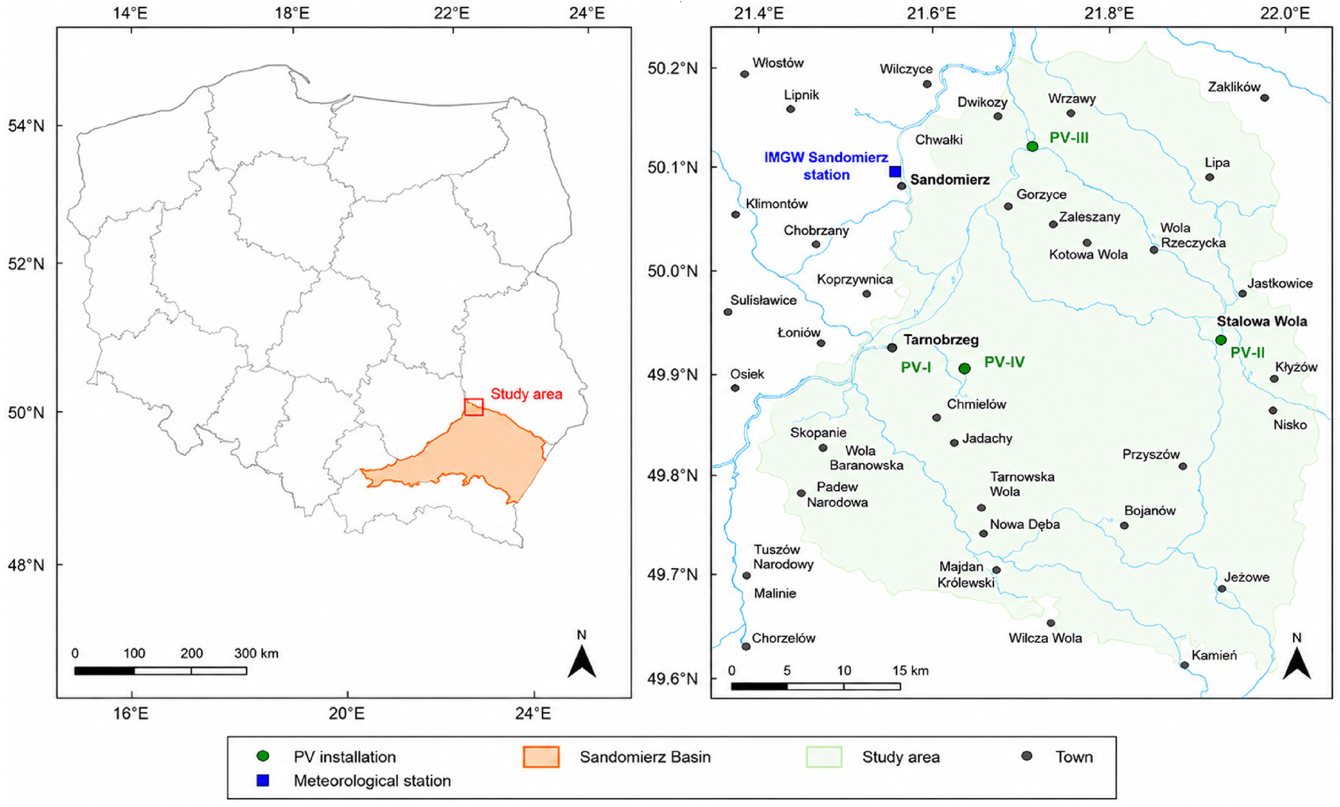
The study covered four prosumer photovoltaic microinstallations located in the northern part of the Podkarpackie Voivodeship, within the Sandomierz Basin in southeastern Poland. Two installations were located in Tarnobrzeg, one in Stalowa Wola, and one in Wrzawy. All analyzed facilities were rooftop installations operating under real prosumer conditions. The locations of the analyzed microinstallations and the meteorological reference point are shown in Figure 1. For the analysis, a common meteorological reference point was adopted: the IMGW Sandomierz station, located approximately 15–30 km from the studied installations. Using a single meteorological station enabled monthly energy production to be related consistently to sunshine duration and air temperature in the region. The meteorological variables were therefore treated as regional reference data rather than as exact site-specific exposure measurements. No correction for local microclimatic differences was applied because parallel meteorological observations were not available for the individual PV locations. Sunshine duration is not equivalent to plane-of-array irradiance and was not treated as a substitute for direct irradiance measurements at the PV arrays. In the statistical analyses, it was used only as a regional meteorological proxy describing the temporal variability of solar-resource conditions. At the same time, this approach does not eliminate possible local differences among the sites resulting, among other factors, from surrounding buildings, roof exposure, shading, ventilation, or the immediate surroundings of the installations.

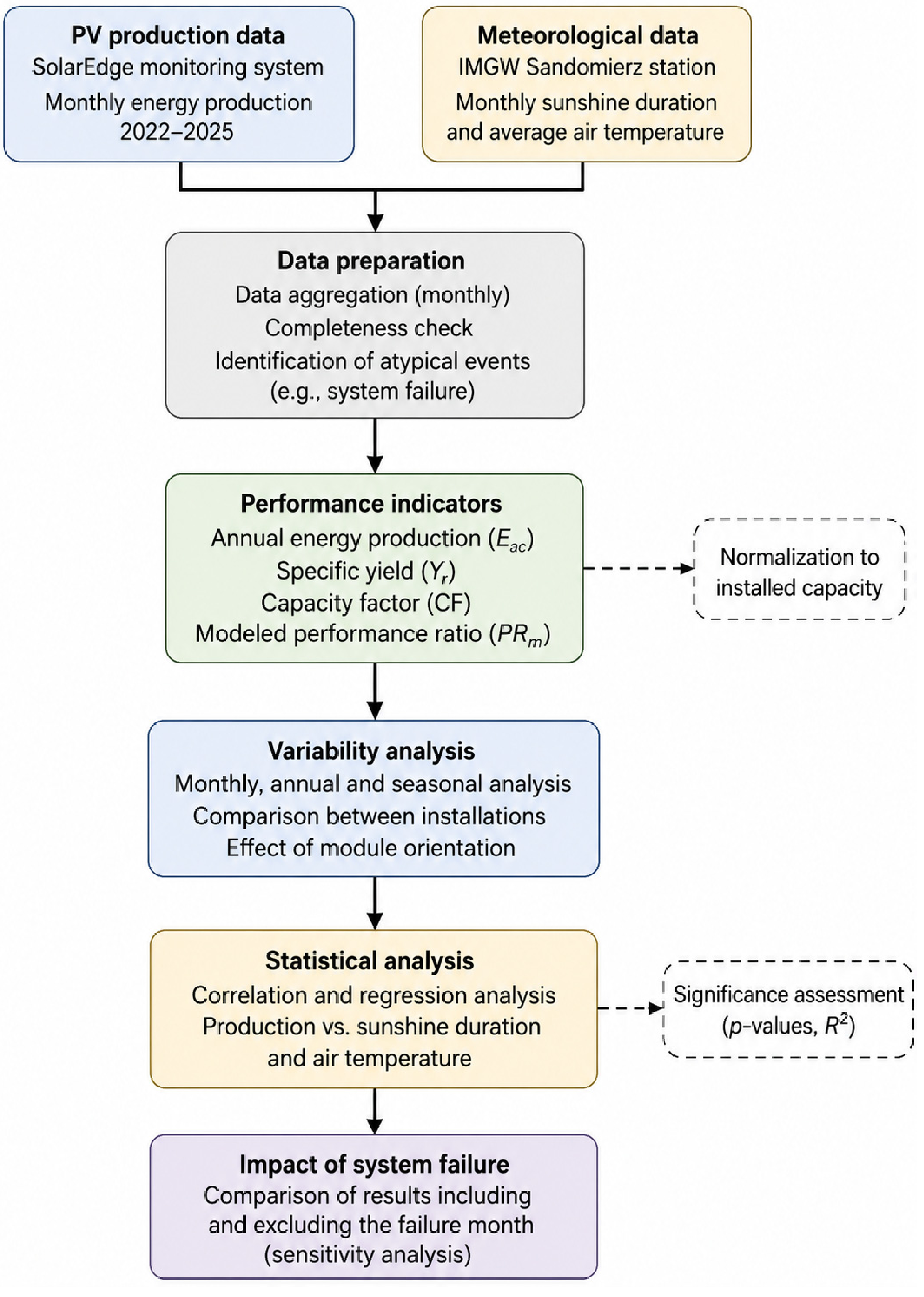
The analysis was based on monthly electricity-production data from the SolarEdge monitoring system and monthly meteorological data covering sunshine duration and mean air temperature from the IMGW Sandomierz station. The study period covered 2022–2025. Production data were combined with the technical parameters of the installations, particularly nominal capacity and module orientation, which enabled comparison of systems with different technical configurations. The general analytical procedure is presented in Figure 2. In the first stage, monthly production and meteorological data were collected and organized. Data completeness was then checked, and atypical events were identified, including the month in which one installation produced no energy because of a failure. Next, productivity indicators were calculated, including annual energy production, specific yield, capacity factor, and the model-based PR_AP estimate. Monthly, annual, and seasonal analyses were then performed, and relationships between energy production and sunshine duration and air temperature were assessed using correlation and regression. For the installation affected by the failure, results from the complete dataset were additionally compared with results obtained after excluding the failure month.

2.2. Characteristics of the PV Installations

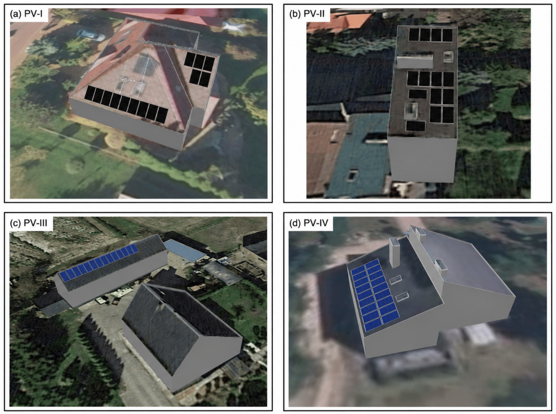
Four grid-connected prosumer photovoltaic microinstallations installed on the roofs of single-family houses were analyzed. All systems were fixed, three-phase installations operating on-grid without physical energy storage. The analyzed systems were equipped with SolarEdge Technologies Ltd. (Herzliya, Israel) inverters and module-level power optimizers. The optimizers reduce the effect of electrical mismatch among individual modules and partial shading on the operation of the entire module string, although they do not completely eliminate losses resulting from local installation and operating conditions. Energy production was recorded in the SolarEdge monitoring system, which enabled monthly energy-yield values to be compiled for all analyzed installations. For the purposes of this article, the installations were assigned the codes PV-I, PV-II, PV-III, and PV-IV, which are used consistently throughout the paper, in the tables, figures, and statistical analyses. These codes serve only for identification and do not indicate a hierarchy or an assessment of system quality. The installations were equipped with three-phase SolarEdge inverters with nominal AC power ratings of 5 kW for PV-I, 4 kW for PV-II, and 5 kW for PV-III and PV-IV, together with module-level power optimizers. Installation capacity is reported as the nominal installed DC-side capacity, expressed in kWp. The analyzed microinstallations form two comparison groups in terms of nominal capacity. Systems PV-I and PV-II had the same installed capacity of 4.69 kWp and used 14 Astronergy CHSM60-HC-335 monocrystalline modules rated at 335 W each (Haining, Zhejiang, China). However, they differed in location, optimizer type, inverter capacity, and module orientation: PV-I faced south, whereas PV-II faced southwest. The rooftop layout and arrangement of PV modules in the analyzed systems are shown in Figure 3.

The second group comprised PV-III and PV-IV, each with a capacity of 5.04 kWp. PV-III, located in Wrzawy, consisted of 14 Longi LR4-60HPH-360M monocrystalline modules rated at 360 W each and faced southeast (Xi’an, Shaanxi, China). PV-IV, located in Tarnobrzeg, consisted of 18 CHSM6610P-280 Astro Halo polycrystalline modules rated at 280 W each and faced west (Haining, Zhejiang, China). In this comparison pair, the same nominal capacity was achieved using different numbers of modules. The set of analyzed installations makes it possible to assess the real-world productivity of PV systems in a comparative framework in which nominal capacity is not the only factor differentiating system operation. The technical characteristics of the analyzed microinstallations are presented in

Table 1. Technical characteristics of the analyzed PV microinstallations based on source documentation (mono-Si, monocrystalline modules; poly-Si, polycrystalline modules).

Code	Location	Capacity (kWp)	Modules	Technology	Azimuth	Tilt Angle [°]	Optimizer	Inverter
PV-I	Tarnobrzeg	4.69	14 × 335 W Astronergy CHSM60-HC-335	mono-Si	S	35	SolarEdge P505	SolarEdge SE5K
PV-II	Stalowa Wola	4.69	14 × 335 W Astronergy CHSM60-HC-335	mono-Si	SW	37	SolarEdge P404	SolarEdge SE5K
PV-III	Wrzawy	5.04	14 × 360 W Longi LR4-60HPH-360M	mono-Si	SE	39	SolarEdge P404	SolarEdge SE5K
PV-IV	Tarnobrzeg	5.04	18 × 280 W CHSM6610P-280 Astro Halo	poly-Si	W	27	SolarEdge P300	SolarEdge SE5K

.

2.3. Production and Meteorological Data

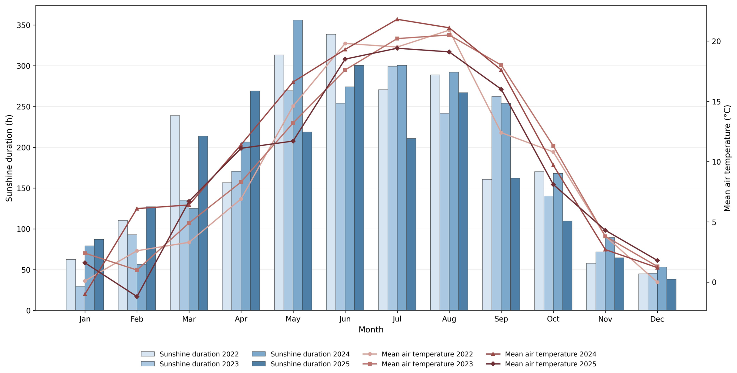
The analysis covered the period from January 2022 to December 2025. Monthly AC electricity production values obtained from the SolarEdge monitoring system were used for each of the four installations. Hourly production data were not available for this study. In total, the dataset contained 48 monthly observations for each installation, or 192 installation–month observations. Production data were treated as AC electricity recorded by the monitoring system at the whole-installation level. For PV-IV, no energy production was recorded in August 2024 because of a system failure. This observation was marked in the dataset as an atypical event. It was subsequently used to determine the extent to which a single failure month affected average productivity indicators. The meteorological data comprised monthly sunshine-duration totals and mean monthly air temperatures from the IMGW Sandomierz station. These variables characterize regional monthly meteorological conditions and do not represent the irradiance incident on the plane of the individual PV arrays. Annual sunshine-duration totals were 2213.2 h in 2022, 2012.8 h in 2023, 2254.5 h in 2024, and 2068.8 h in 2025. The highest annual sunshine duration was recorded in 2024 and the lowest in 2023. Differences among years indicate clear variability in meteorological conditions during the analysis period, justifying comparison of PV production with sunshine-duration and air-temperature data. The meteorological data were used as a common reference background for all analyzed installations. This approach ensures consistency in comparisons among systems but does not fully capture local microclimatic differences that may have occurred among Tarnobrzeg, Stalowa Wola, Wrzawy, and Sandomierz. Annual meteorological conditions are summarized in

Table 2. Annual meteorological characteristics from the Sandomierz station used in the analysis.

Year	Sunshine Duration (h)	Mean Temperature (°C)
2022	2213.2	9.56
2023	2012.8	10.21
2024	2254.5	11.08
2025	2068.8	9.76

, and their monthly variability is shown in Figure 4.

2.4. Indicators for Assessing Energy Productivity and Seasonality

Differences in the nominal capacities of the analyzed microinstallations prevent meaningful comparison based solely on absolute energy production. Therefore, the results were normalized by the nominal installed DC-side capacity of the PV generator. The analysis used specific yield, capacity factor, the seasonal structure of production, and a supplementary indicator relating actual production to model-estimated solar-radiation resources. The methodological origin of each indicator is specified below, distinguishing IEC-defined metrics from indicators adapted or calculated for the purposes of this study.

The primary productivity indicator was the specific yield, Y_f, corresponding to the final PV-system yield defined in IEC 61724-1 [36]:

Y_f = E_AC/P₀

(1)

where

• Y_f—specific yield during the analyzed period [kWh/kWp];
• E_AC—AC electricity production during the analyzed period [kWh];
• P₀—nominal installed DC-side capacity of the PV generator [kWp].

Specific yield was calculated monthly and annually. This indicator enables installations with different nominal capacities to be compared but is not a direct measure of the efficiency of converting solar-radiation energy into electricity.

The capacity factor (CF), a commonly used energy-performance indicator, was calculated as the ratio of actual energy production to the energy that the installation could have produced if it had operated at nominal capacity throughout the analyzed period [49]:

CF = E_AC/(P₀ × t) × 100%

(2)

where

• CF—capacity factor during the analyzed period [%];
• t—number of hours in the analyzed period [h].

For annual calculations, 8760 h was used for 2022, 2023, and 2025, and 8784 h for the leap year 2024. For monthly analyses, the actual number of hours in each month was used.

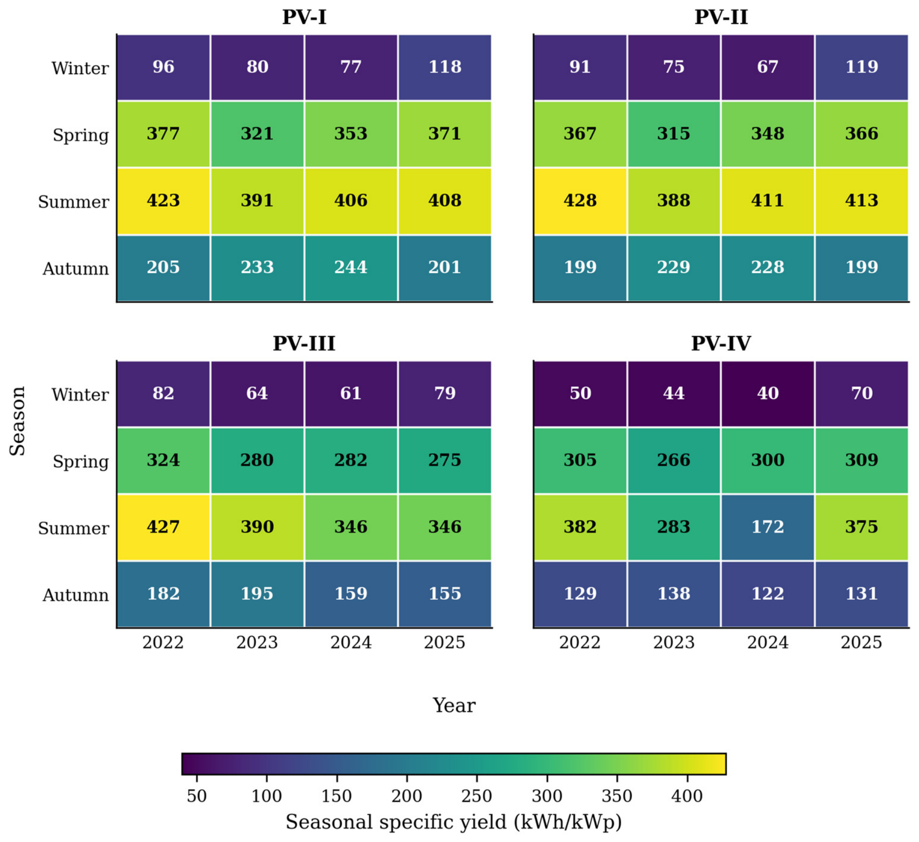
For the comparative purposes of this study, the seasonal structure of production was determined from the share of energy produced in a given season in the total energy production of the analyzed installation:

fs = E_AC,s/E_AC,tot × 100%

(3)

where

• f_s—share of energy production in season s [%];
• E_AC,s—energy produced during the months included in season s [kWh];
• E_AC,tot—total energy production during 2022–2025 [kWh];
• s—season (winter, spring, summer, or fall).

The following seasonal division was adopted: winter—December, January, and February; spring—March, April, and May; summer—June, July, and August; fall—September, October, and November. Seasonal shares were calculated separately for each microinstallation using data from the entire study period.

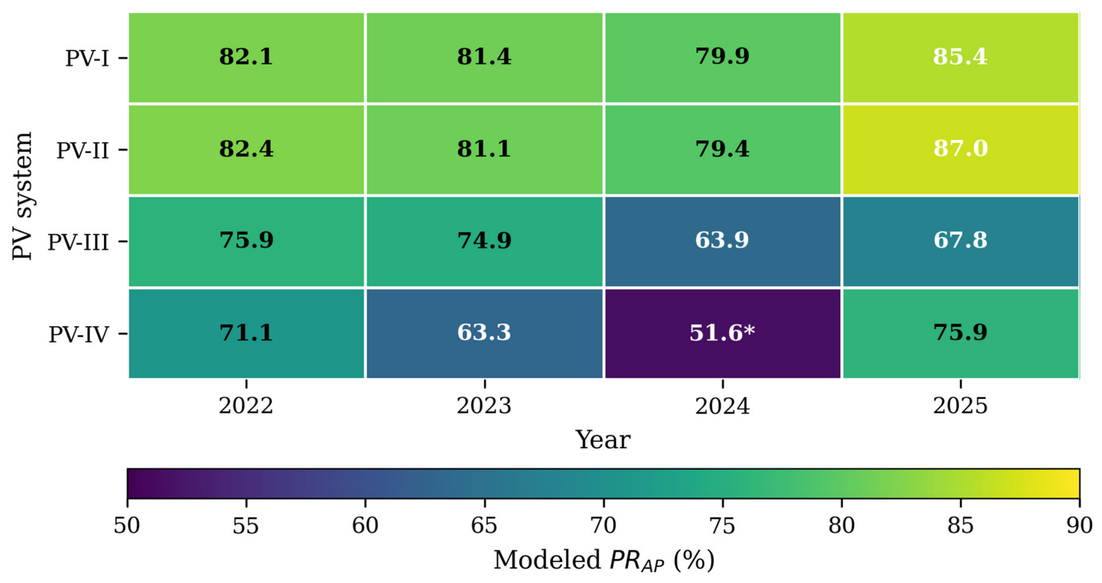
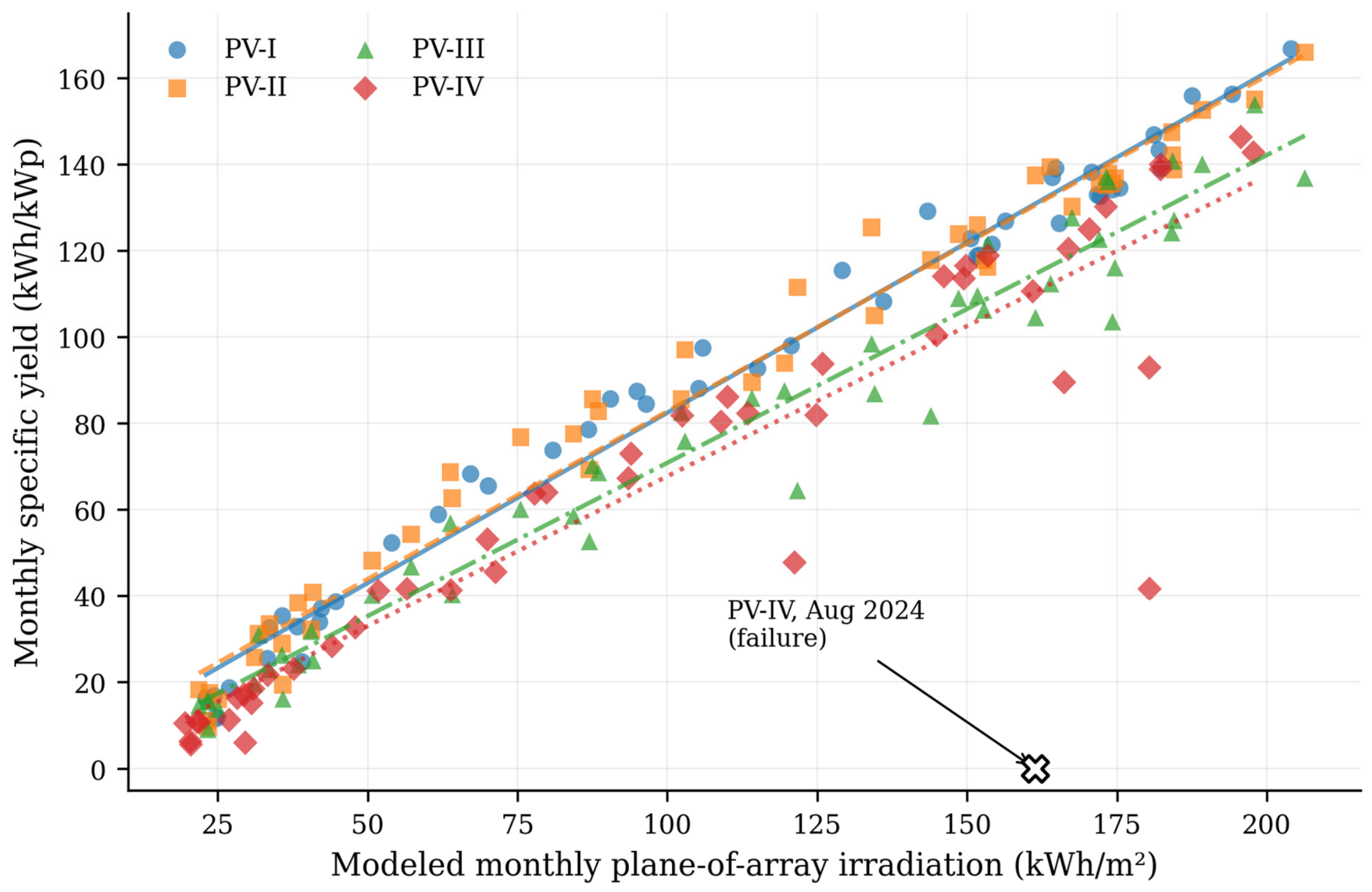
The performance ratio is defined in IEC 61724-1 [36]. However, because plane-of-array irradiation was not measured directly at the analyzed installations, the present study used a model-based adaptation of this indicator. The actual specific yield was related to the model-estimated plane-of-array irradiation, H_POA,AP, obtained from the adopted irradiation model [50]. On this basis, the model-based performance-ratio estimate, PR_AP, was calculated:

PR_AP = Y_f/(H_POA,AP/G_STC) × 100%

(4)

where

• PR_AP—model-based estimate of the performance ratio calculated using model-estimated plane-of-array irradiation during the analyzed period [%];
• Y_f—specific yield during the analyzed period [kWh/kWp];
• H_POA,AP—model-estimated plane-of-array irradiation during the analyzed period [kWh/m²];
• G_STC—reference irradiance under STC, equal to 1 kW/m².

PR_AP estimates were used only as a supplementary comparative indicator among the analyzed installations. Because plane-of-array irradiation was model-estimated rather than measured directly at the PV arrays, PR_AP should not be interpreted as a conventional measurement-based performance ratio or as a direct measure of total system losses.

2.5. Statistical Analysis

EC 61724-1 provides the methodological framework for PV-system monitoring and the calculation of standardized performance metrics [36]. The subsequent data analyses applied in this study, including monthly and seasonal comparisons, Pearson correlation, ordinary least-squares regression, hierarchical multiple regression, and sensitivity analysis of the documented failure event, were selected by the authors to address the specific objectives of the study and are not analytical procedures prescribed by IEC 61724-1.

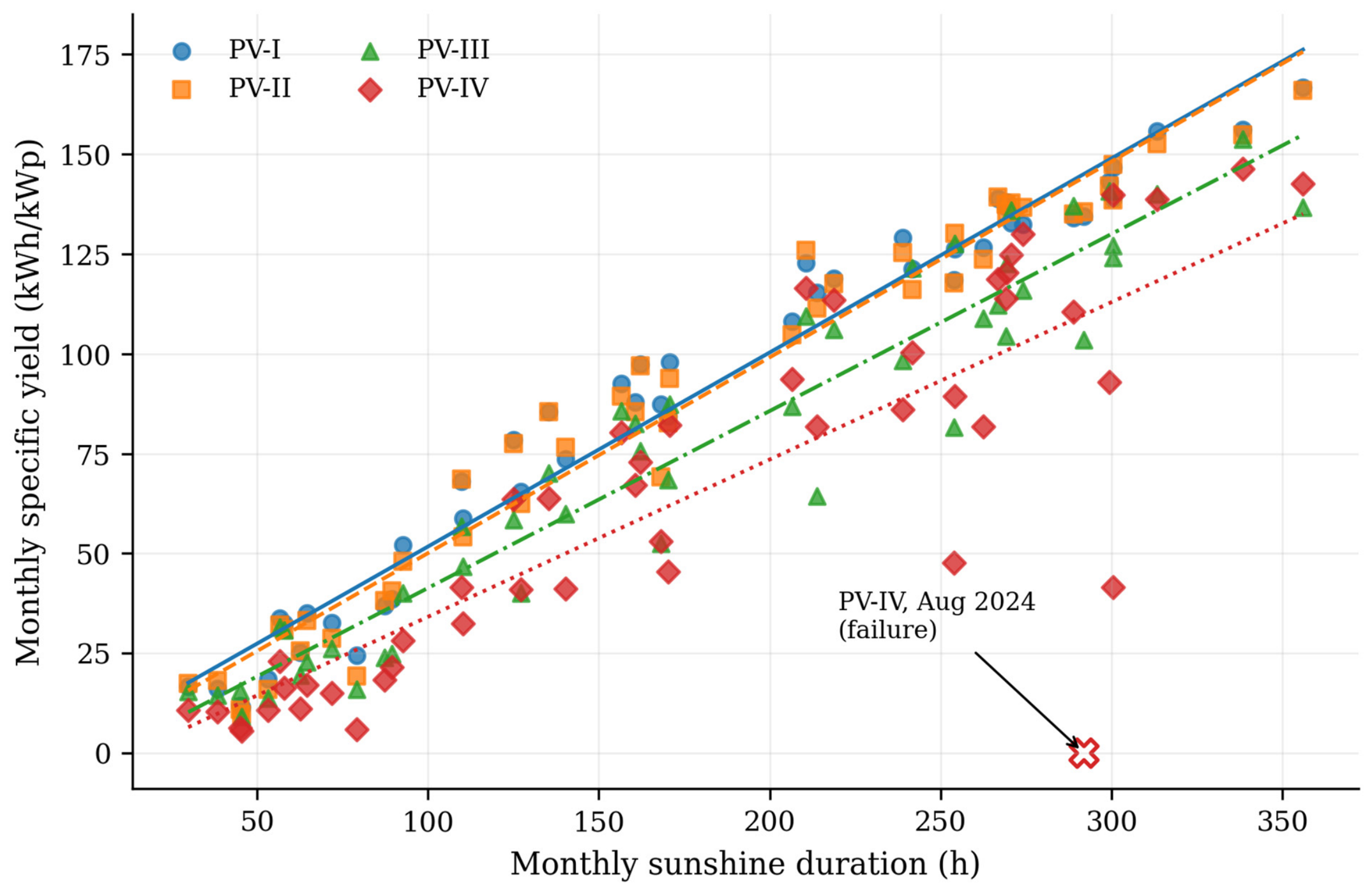
Relationships between meteorological conditions and microinstallation productivity were assessed using monthly data from 2022 to 2025. Sunshine duration was included as a regional temporal proxy for solar-resource conditions and not as a substitute for measured plane-of-array irradiance. For each installation, Pearson’s correlation coefficient was calculated between monthly specific yield and sunshine duration and mean air temperature. The number of observations for each installation was n = 48. Statistical significance was assessed at α = 0.05.

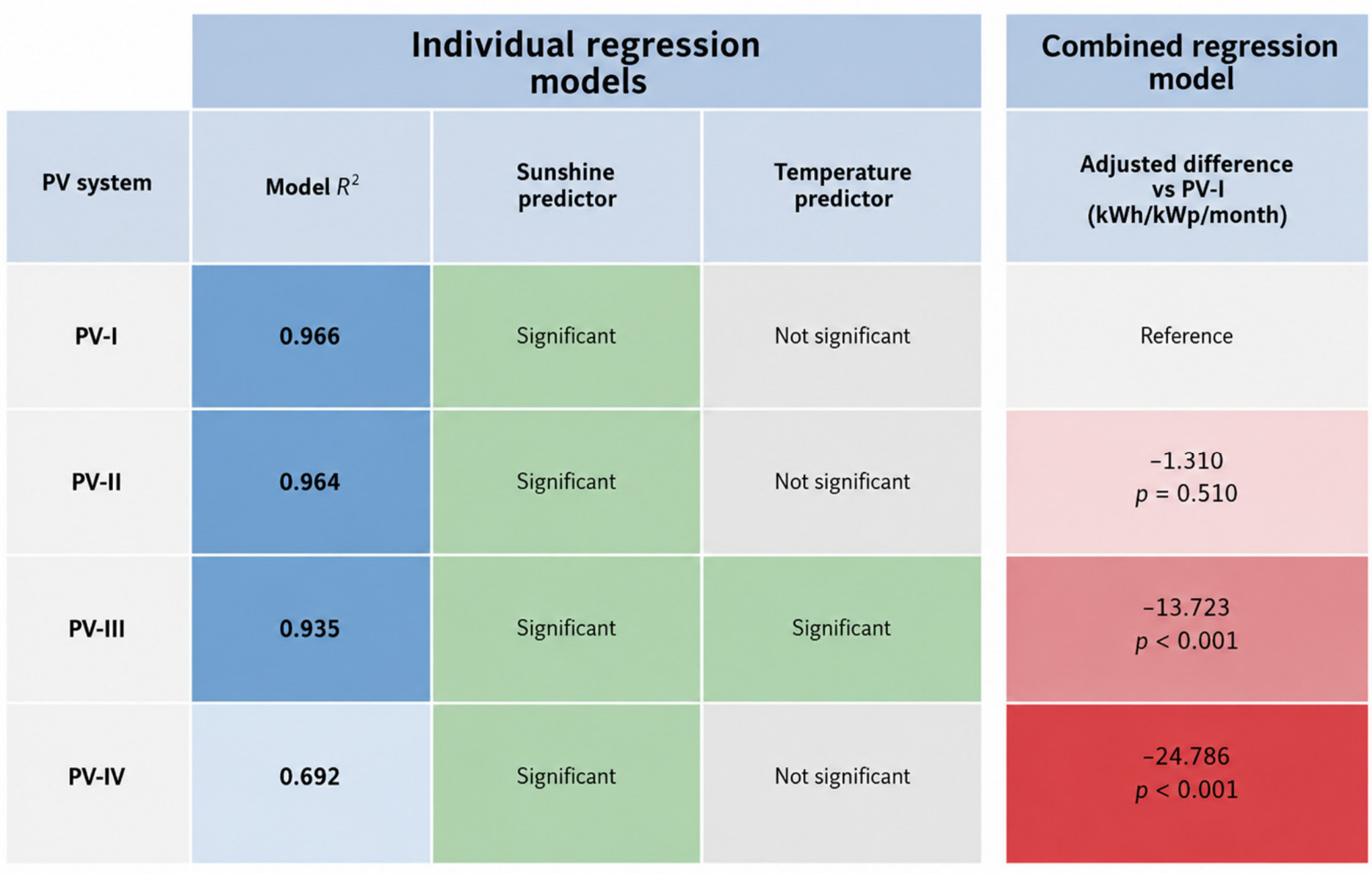
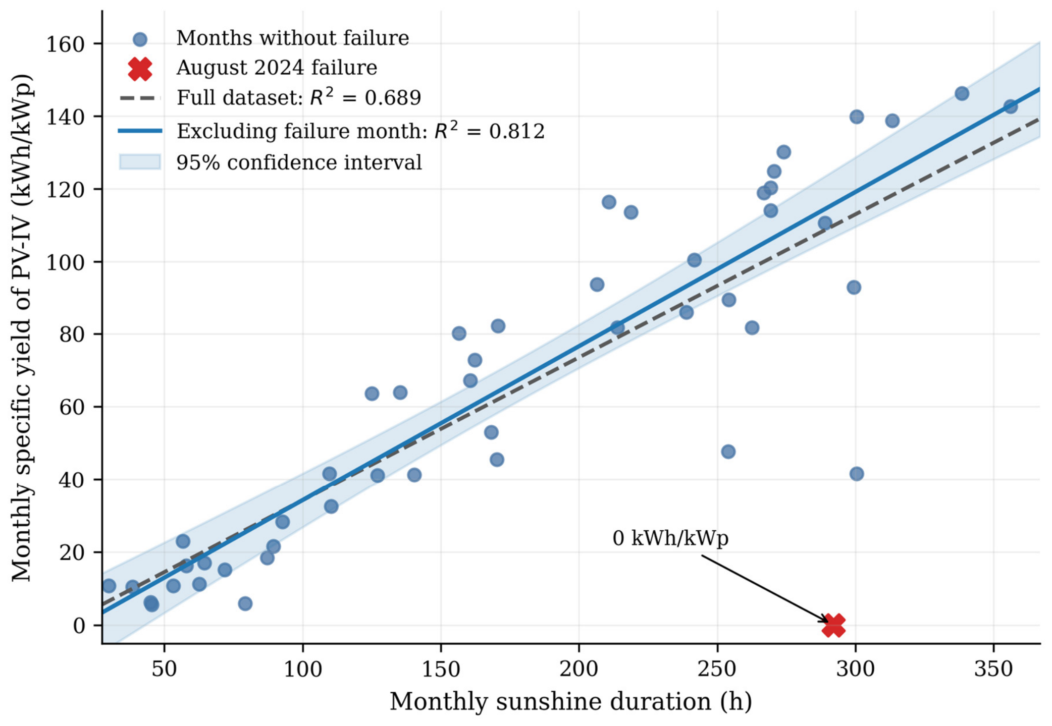
For each installation, regression analysis was performed for specific yield as a function of sunshine duration and air temperature. A combined analysis was also performed for all installations, and model fit was evaluated using the coefficient of determination, R². Accordingly, the regression coefficients quantify statistical associations within the analyzed dataset and should not be interpreted as physical response coefficients to site-specific irradiance. The effect of the PV-IV failure was assessed by comparing results for the complete dataset with those obtained after excluding the August 2024 observation.

To evaluate the incremental contribution of installation-specific, seasonal, and failure-related variables, the combined regression described above was extended hierarchically. Model 1 included sunshine duration and mean air temperature. Model 2 added installation dummy variables, with PV-I as the reference category. Model 3 additionally included season, with winter as the reference category, and Model 4 included failure status, coded as 1 for PV-IV in August 2024 and 0 otherwise. For each model, unstandardized coefficients, R², adjusted R², and ΔR² were reported. Statistical significance of the regression coefficients was indicated using p-value thresholds. Multicollinearity was assessed using variance inflation factors.

3. Results

3.1. Annual Energy Production and Normalized Indicators

Annual energy production varied among installations and years. For PV-I, it ranged from 4.818 to 5.164 MWh/year, with the minimum in 2023 and the maximum in 2022. For PV-II, the range was 4.725–5.144 MWh/year; the lowest value was recorded in 2023 and the highest in 2025. PV-III produced from 4.288 MWh in 2024 to 5.034 MWh in 2022, whereas PV-IV produced from 3.201 MWh in 2024 to 4.463 MWh in 2025. Mean production values and normalized indicators are presented in

Table 3. Mean annual energy production (mean ± SD, n = 4 years) and normalized indicators for PV-I–PV-IV during 2022–2025.

Installation	Mean Production (MWh/Year)	Capacity (kWp)	Mean Specific Yield (kWh/kWp/Year)	Capacity Factor, CF (%)	Orientation	Technology
PV-I	5.054 ± 0.162	4.69	1077.7	12.30	S	mono-Si
PV-II	4.979 ± 0.186	4.69	1061.7	12.12	SW	mono-Si
PV-III	4.580 ± 0.355	5.04	908.6	10.37	SE	mono-Si
PV-IV	3.929 ± 0.594	5.04	779.6	8.90	W	poly-Si

. PV-I achieved mean production of 5.054 ± 0.162 MWh/year, a mean specific yield of 1077.7 kWh/kWp/year, and a CF of 12.30%. For PV-II, the corresponding values were 4.979 ± 0.186 MWh/year, 1061.7 kWh/kWp/year, and 12.12%. The difference in mean specific yield between PV-I and PV-II, which had the same nominal capacity, was 16.0 kWh/kWp/year, or 1.5%. PV-III achieved a mean of 908.6 kWh/kWp/year with a CF of 10.37%, whereas PV-IV achieved 779.6 kWh/kWp/year with a CF of 8.90%. Within the pair of 5.04 kWp installations, the mean yield of PV-IV was 129.0 kWh/kWp/year, or 14.2% lower than that of PV-III.

Annual specific yield is shown in Figure 5. PV-I and PV-II maintained similar levels in each year; the difference between them ranged from 1.9 kWh/kWp in 2025 to 25.9 kWh/kWp in 2024. Both installations reached their minimum in 2023, and in 2025 the values increased to 1098.7 kWh/kWp for PV-I and 1096.8 kWh/kWp for PV-II. The yield of PV-III decreased from 998.8 kWh/kWp in 2022 to 850.8 kWh/kWp in 2024 and remained at a similar level in 2025 (854.6 kWh/kWp). PV-IV reached a minimum of 635.1 kWh/kWp in 2024, which included the failure month, and increased to 885.5 kWh/kWp in 2025. Throughout the study period, PV-I and PV-II achieved the highest and most stable specific yields, whereas PV-IV showed the greatest interannual variability.

3.2. Monthly Profile and Seasonal Production Structure

Mean monthly specific-yield profiles, calculated from four years of observations, are shown in Figure 6. The highest value for PV-I occurred in May (144.8 kWh/kWp/month), and PV-II also peaked in May (142.9 kWh/kWp/month). PV-III reached its maximum in June at 130.3 kWh/kWp/month, whereas PV-IV reached its highest mean value in May (128.8 kWh/kWp/month). The lowest mean yields for all systems occurred in December, ranging from 8.2 kWh/kWp/month for PV-IV to 14.6 kWh/kWp/month for PV-I.

The profiles of PV-I and PV-II were similar throughout the year, although PV-II slightly exceeded PV-I in June and July. Monthly differences between these installations did not exceed 4.1 kWh/kWp. PV-III achieved lower values mainly from July through November, whereas the greatest differences between PV-IV and the other systems occurred from July through October. The mean August yield of PV-IV was 82.4 kWh/kWp, compared with 132.2 kWh/kWp for PV-I. The lower mean value for PV-IV was associated with zero energy production in August 2024.

Seasonal production shares over the entire study period are presented in

Table 4. Seasonal share of energy production for PV-I–PV-IV over the entire 2022–2025 study period.

Installation	Winter (%)	Spring (%)	Summer (%)	Fall (%)
PV-I	8.6	33.1	37.8	20.5
PV-II	8.3	32.9	38.6	20.1
PV-III	7.8	31.8	41.4	19.0
PV-IV	6.5	37.9	38.9	16.7

. Summer accounted for the largest share of production for PV-I, PV-II, and PV-III, at 37.8%, 38.6%, and 41.4%, respectively. For PV-IV, the spring and summer shares were similar, at 37.9% and 38.9%. Winter accounted for the smallest share of energy production for each installation, ranging from 6.5% for PV-IV to 8.6% for PV-I. The combined spring and summer shares were 70.9% for PV-I, 71.6% for PV-II, 73.2% for PV-III, and 76.7% for PV-IV.

For PV-I and PV-II, summer yield remained within ranges of 390.8–423.0 and 388.2–427.7 kWh/kWp, respectively. For PV-III, summer yield decreased from 426.7 kWh/kWp in 2022 to 345.8 kWh/kWp in 2025. The greatest change was recorded for PV-IV: the summer value was 381.6 kWh/kWp in 2022, 282.6 kWh/kWp in 2023, 171.6 kWh/kWp in 2024, and 375.0 kWh/kWp in 2025. All installations had their lowest values in winter, whereas the highest winter values occurred in 2025 (Figure 7).

3.3. Model-Based Estimate of the Performance Ratio (PR_AP)

Model-estimated plane-of-array irradiation was used only as a reference value for calculating the PR_AP estimate. This estimate describes the relationship between actual specific yield and the reference yield resulting from the adopted irradiation resource. Mean PR_AP estimates for PV-I and PV-II were 82.2% and 82.5%, respectively, meaning that their actual specific yields were approximately 82% of the reference yield. For PV-III, the indicator reached 70.6%, which was 11.6 percentage points lower than for PV-I and 11.9 percentage points lower than for PV-II, whereas for PV-IV it was 65.5%. The comparison of PV-II and PV-III was particularly important: the same mean model-estimated irradiation value of 1287.9 kWh/m²/year was adopted for both installations, but the actual specific yield of PV-III was 153.1 kWh/kWp/year lower. This corresponded to a difference of 11.9 percentage points in PR_AP, indicating that the productivity difference between these installations cannot be explained solely by the adopted irradiation-resource level. For PV-IV, the lower reference yield was also accompanied by the largest relative gap between actual and reference yield. Because of the model-based nature of the reference value, the difference from 100% was not interpreted as a directly measured total system loss. Detailed results are presented in

Table 5. Mean values and interannual variability of the model-based PRAP indicator. Mean estimates and interannual variability of the model-based performance-ratio estimate (PR_AP) for PV-I–PV-IV.

Installation	Azimuth	Mean Specific Yield (kWh/kWp/Year)	Mean HPOA,AP  (kWh/m2/Year)	Mean PRAP ± SD (%)
PV-I	S	1077.7	1311.8	82.2 ± 2.3
PV-II	SW	1061.7	1287.9	82.5 ± 3.3
PV-III	SE	908.6	1287.9	70.6 ± 5.8
PV-IV	W	779.6	1192.6	65.5 ± 10.6

.

Interannual PR_AP estimates are shown in Figure 8. In 2024, all installations reached their lowest indicator values, even though model-estimated plane-of-array irradiation was highest in that year. This means that the increase in the reference resource was not accompanied by a proportional increase in actual yield. The decrease was small for PV-I and PV-II, whereas the value for PV-III fell to 63.9%. The strongest deviation occurred for PV-IV, for which PR_AP was 51.6%; this result included the month of zero production. In 2025, the indicator increased to 85.4% for PV-I, 87.0% for PV-II, 67.8% for PV-III, and 75.9% for PV-IV.

Monthly specific yield increased with increasing model-estimated plane-of-array irradiation for all analyzed installations. Observations for PV-I and PV-II formed similar point clouds and remained at the highest yield level over almost the entire irradiation range. PV-III achieved a lower specific yield than PV-II even though identical monthly irradiation values were adopted for both installations, indicating that the difference between them persisted after production was related to the same reference resource. PV-IV showed both the lowest yield values and the greatest dispersion of observations, particularly at higher irradiation levels. The point corresponding to August 2024 clearly differed from the remaining data because zero production was recorded at a high irradiation value as a result of the failure. The separate fitted lines for the installations show that differences in their productivity cannot be explained solely by variability in the model-estimated irradiation resource (Figure 9).

3.4. Meteorological Determinants of Specific Yield

Monthly specific yield was most strongly associated with sunshine duration. Pearson’s correlation coefficient was r = 0.983 for PV-I, 0.981 for PV-II, 0.960 for PV-III, and 0.830 for PV-IV; all relationships were statistically significant (p < 0.001; n = 48 for each installation). Correlations with mean monthly air temperature were also positive but weaker: r = 0.857 for PV-I, 0.866 for PV-II, 0.889 for PV-III, and 0.697 for PV-IV (p < 0.001). The distribution of monthly observations relative to sunshine duration is shown in Figure 10. For PV-I and PV-II, the points and fitted lines remained close throughout the sunshine-duration range. PV-III formed a lower set of observations, particularly at values exceeding 200 h/month. The greatest dispersion was found for PV-IV; in addition to the failure month, observations with high sunshine duration and yields below the trend line were also visible. In August 2024, zero specific yield was recorded with 292.0 h of sunshine duration.

Regression models including sunshine duration and air temperature, estimated separately for each installation, explained 96.6% of the variability in monthly specific yield for PV-I, 96.4% for PV-II, 93.5% for PV-III, and 69.2% for PV-IV. Sunshine duration was a positive and significant predictor in all four models. Temperature reached the significance level only in the PV-III model; its effect was not statistically significant in the PV-I, PV-II, and PV-IV models. The combined model included 192 installation–month observations and explained 88.8% of the variability in monthly specific yield (R² = 0.888). The coefficient for sunshine duration was β = 0.432 (p < 0.001), whereas the temperature coefficient was β = 0.309 (p = 0.310). After sunshine duration and temperature were included, the predicted monthly yield of PV-II was, on average, 1.310 kWh/kWp lower than that of PV-I, but this difference was not statistically significant (p = 0.510). For PV-III and PV-IV, yield was lower than for PV-I by 13.723 and 24.786 kWh/kWp/month, respectively, and these differences were statistically significant (p < 0.001). The two stages of the regression analysis are summarized in Figure 11. The “Individual regression models” section summarizes the models estimated separately for each installation, whereas the “Combined regression model” section presents adjusted differences in monthly yield relative to PV-I obtained from the combined model including 192 installation–month observations.

To further distinguish the incremental explanatory contribution of meteorological, installation-specific, seasonal, and failure-related variables, the combined dataset was analyzed using hierarchical multiple regression. The combined regression model presented in Figure 11 corresponds to Model 2 of the hierarchical analysis reported in

Table 6. Hierarchical multiple regression models for monthly specific yield in the combined dataset.

Predictor/Statistic	Model 1	Model 2	Model 3	Model 4
Intercept	−0.386	9.568 **	12.150 ***	11.440 ***
Sunshine duration (h)	0.432 ***	0.432 ***	0.314 ***	0.314 ***
Mean air temperature (°C)	0.309	0.309	1.097 *	1.165 **
PV-II vs. PV-I	—	−1.310	−1.310	−1.310
PV-III vs. PV-I	—	−13.723 ***	−13.723 ***	−13.723 ***
PV-IV vs. PV-I	—	−24.786 ***	−24.786 ***	−22.283 ***
Spring vs. winter	—	—	24.876 ***	24.323 ***
Summer vs. winter	—	—	13.481 *	14.736 **
Fall vs. winter	—	—	3.651	3.071
Failure status	—	—	—	−120.130 ***
R2	0.842	0.888	0.910	0.943
Adjusted R2	0.840	0.885	0.906	0.940
ΔR2	—	0.047	0.021	0.033
ΔR2 p-value	—	<0.001	<0.001	<0.001

Values are unstandardized regression coefficients. PV-I and winter were the reference categories. Failure status was coded as 1 only for PV-IV in August 2024 and 0 otherwise. * p < 0.05, ** p < 0.01, *** p < 0.001. ΔR² represents the increase in explained variance relative to the preceding model.

, which summarizes the successive models, their explanatory power, and changes in model fit. Meteorological variables alone explained 84.2% of the variability in monthly specific yield. Adding installation effects increased R² by 0.047 (p < 0.001), seasonal effects added 0.021 (p < 0.001), and the documented failure added a further 0.033 (p < 0.001), yielding a final R² of 0.943. In the final model, sunshine duration, mean air temperature, PV-III, PV-IV, spring, summer, and failure status were significant, whereas PV-II and fall were not. The installation coefficients represent adjusted differences among the analyzed systems and should not be interpreted as independent causal effects of orientation, because each orientation was represented by only one installation.

3.5. Effect of the PV-IV Failure on the Analysis Results

The effect of the August 2024 failure observation on the relationship between sunshine duration and PV-IV specific yield is shown in Figure 12. For the complete dataset of 48 months, the correlation coefficient was r = 0.830, and the coefficient of determination was R² = 0.689. After the failure month was excluded, these values increased to r = 0.901 and R² = 0.812, respectively, at n = 47. The coefficient of determination therefore increased by 0.123, or 12.3 percentage points, corresponding to a relative increase of 17.8%. The failure observation lay clearly below the remaining points and lowered the regression line at high sunshine duration. After it was excluded, the fitted line ran closer to the main cluster of observations, and the 95% confidence interval was calculated from the remaining 47 months of observations.

After the failure observation was excluded, the number of observations in the complete dataset (all installations) decreased to 191, and model fit increased to R² = 0.921. The sunshine-duration coefficient remained virtually unchanged (β = 0.430; p < 0.001), whereas the temperature coefficient increased to β = 0.459 but still did not reach the significance level (p = 0.081). The PV-II effect remained nonsignificant (−1.310 kWh/kWp/month; p = 0.500), the PV-III effect was −13.723 kWh/kWp/month (p < 0.001), and the absolute value of the PV-IV effect decreased from −24.786 to −22.255 kWh/kWp/month (p < 0.001). Excluding the failure month improved model fit but did not change the direction or significance of the main differences among the analyzed installations.

4. Discussion

Assessment of the real-world operation of PV microinstallations should not be based solely on nominal capacity because it does not directly reflect energy performance. System productivity results from the combined effects of the solar resource, mounting geometry, technology, local surroundings, and continuity of operation [51,52,53,54]. In the analyzed dataset, PV-I and PV-II, each rated at 4.69 kWp, achieved both higher mean annual production and higher specific yield than PV-III and PV-IV, each rated at 5.04 kWp. This result confirms that greater installed capacity alone does not guarantee more energy per 1 kWp or better use of the available resource.

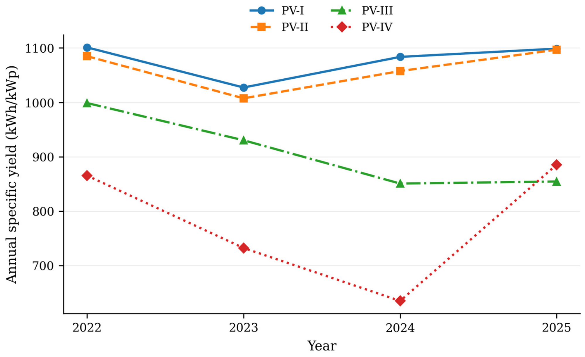
The mean specific yield was 1077.7 kWh/kWp/year for PV-I and 1061.7 kWh/kWp/year for PV-II, whereas PV-III and PV-IV achieved 908.6 and 779.6 kWh/kWp/year, respectively. These values fall within the range of variation observed in actual rooftop installations operating in different configurations. Hołota et al. reported yields in Poland ranging from 831 to 1169 kWh/kWp/year, and comparisons of measured and simulated data indicate that differences ranging from more than ten to several tens of percent may also occur among systems operating in similar climatic zones. The results obtained are therefore not unusual for operational PV analyses but demonstrate the scale of differences possible even within a single macroregion [52,55,56,57].

The highest productivity was achieved by south-facing PV-I; however, the yield of southwest-facing PV-II was only 1.5% lower, and after accounting for sunshine duration and temperature, the difference from PV-I was not statistically significant. This agrees with findings indicating that moderate deviation from south usually causes smaller annual losses than east- or west-facing orientation [58]. Optimal geometry also depends on tilt angle and local meteorological conditions [59]; therefore, roof-surface orientation and slope should be considered jointly at the design stage [60]. Southwest-facing configurations may also shift part of production toward the afternoon, which can be beneficial for matching production to demand [61,62]. However, the lower production results of PV-III and PV-IV cannot be attributed solely to their southeast and west orientations, respectively. The comparison of PV-II and PV-III is particularly informative because the same mean model-estimated plane-of-array irradiation was adopted for both installations. Nevertheless, PV-III achieved a yield that was 153.1 kWh/kWp/year lower and a PR_AP estimate that was 11.9 percentage points lower.

The identical annual model-estimated irradiation values do not mean that the two systems operated under identical real conditions or converted the available solar resource into AC electricity in the same way. PV-II and PV-III differed in azimuth, module and inverter configuration, and local installation conditions. Moreover, southeast- and southwest-facing arrays receive peak irradiance at different times of day, so differences in morning and afternoon cloudiness, shading, module temperature, and ventilation may affect their actual yield even when annual modeled irradiation is similar. Shading effects and grid-related voltage constraints are also recognized factors influencing PV-system productivity [63,64]. Because these factors were not monitored separately, their individual effects cannot be determined separately, and the 153.1 kWh/kWp/year difference should be interpreted as the combined effect of installation-specific and local operating conditions rather than orientation alone.

PV-IV also differed from the remaining systems in module technology, using polycrystalline silicon modules, whereas PV-I–PV-III used monocrystalline modules. Differences in module technology may influence long-term operating performance and energy yield under real environmental conditions [65]. However, the lower productivity of PV-IV cannot be attributed independently to module technology because this system also differed in orientation, module model and rating, optimizer configuration, local operating conditions, and experienced the documented failure in August 2024. Module technology should therefore be considered one of several system-specific factors that may have contributed to the observed performance difference.

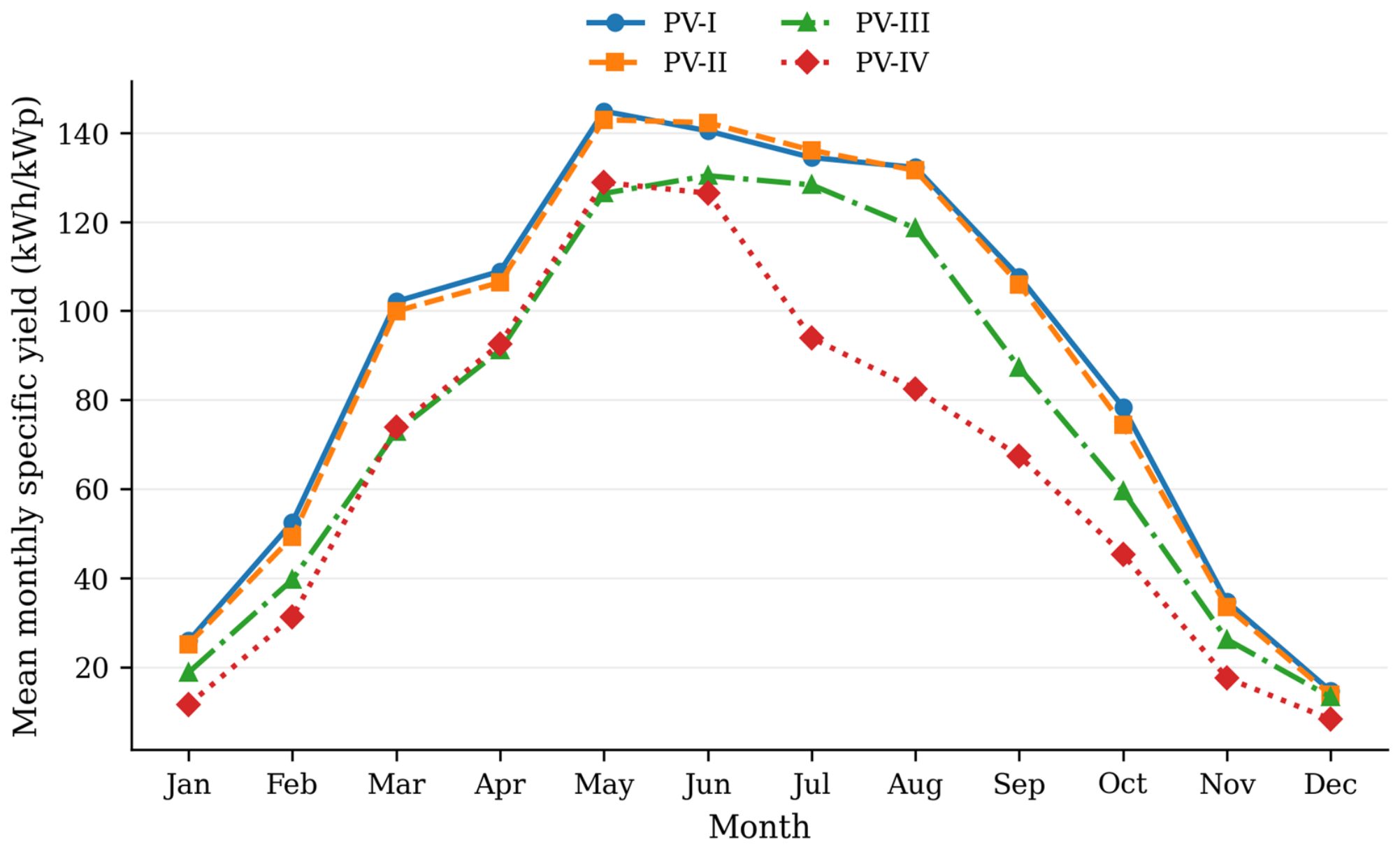
Among the meteorological variables analyzed, monthly sunshine duration showed the strongest relationship with specific yield. Correlation coefficients ranged from r = 0.830 to 0.983, and sunshine duration remained a positive and significant factor in all installation-specific models. This strong monthly association is consistent with the expected seasonal coupling between PV generation and solar-resource conditions; however, sunshine duration itself is not a measure of the irradiance incident on the plane of the PV array [66]. However, a strong monthly relationship does not mean that annual sunshine duration alone is sufficient to predict productivity. In 2024, despite the highest sunshine-duration total, all installations reached their lowest model-based PR_AP estimates. This result confirms the need to verify regional resources and simulation results using operating data [52,55]. The positive correlation between monthly yield and air temperature primarily reflected the common seasonality of the two variables: warmer months were also months with longer sunshine duration. After sunshine duration was included, temperature was not a significant factor in the combined analyses and reached significance only for PV-III in the installation-specific models. This result cannot be interpreted as a beneficial effect of high temperature on modules because increasing cell temperature physically reduces power, and temperature losses may increase discrepancies between measured and simulated production [55,57]. The common IMGW-station data used in this study provided a consistent comparison background but did not fully represent conditions at the plane of each generator. Persistent differences between PV-I/PV-II and PV-III/PV-IV, despite the use of the same regional sunshine-duration data, show that solar-potential maps and meteorological-station data can serve only as reference points and cannot replace local installation monitoring. The lowland-and-valley character of the macroregion justifies such field verification, but without measurements at the installations, lower yields cannot be attributed to specific phenomena such as fog, humidity, or local temperature inversions.

Using specific yield, capacity factor, and the model-based PR_AP estimate made it possible to compare installations independently of their nominal capacities. Installation rankings were similar for specific yield and CF, whereas the PRAP estimate related production to model-estimated irradiation for the adopted orientation. Similar PR_AP estimates for PV-I and PV-II, 82.2% and 82.5%, respectively, indicate a similar relationship between production and the reference resource. Values of 70.6% for PV-III and 65.5% for PV-IV indicate a larger gap from model potential. However, the difference from 100% cannot be interpreted as a directly measured total loss because H_POA,AP was not obtained from sensors installed at the modules [52,55]. The combined regression model, covering data from all installations, explained 88.8% of the variability in monthly yield. After accounting for sunshine duration and temperature, PV-II results did not differ significantly from those of PV-I, whereas PV-III and PV-IV still achieved significantly lower yields. This means that the lower productivity of these installations did not result solely from monthly variation in the common meteorological data. However, the installation effect jointly included all fixed differences among facilities, including orientation, tilt, technology, surroundings, and operating characteristics. The model is therefore comparative and does not allow the observed differences to be causally assigned to a single parameter.

A particularly important result was the quantitative assessment of the effect of the PV-IV failure. After the August 2024 month with no production was excluded from the analyses, the R² of the sunshine-duration–yield relationship increased from 0.689 to 0.812, and the fit of the combined model increased from 0.888 to 0.921. However, the adjusted PV-IV effect remained negative and significant, meaning that the failure worsened the poor result but did not explain the entire difference from PV-I. As indicated in the literature, inverter downtime in other long-term analyses also increased discrepancies between measured and predicted production, and assessment of residential-system reliability required consideration of both degradation and trends in inverter and MPPT-system failures. Failure events should therefore be reported separately and analyzed rather than removed without comment as data errors [67,68]. The results emphasize that monitoring should be part of productivity maintenance, not merely an energy-recording tool. Even simple measurement systems can support identification of atypical operation, whereas effective diagnostics requires appropriate selection of sensors, measurement locations, and sampling frequency [69,70]. Monthly data were sufficient to detect the complete shutdown of PV-IV, but shorter production constraints, voltage-related shutdowns, and gradual performance deterioration require regular review of monitoring data.

In addition to continuity of operation, the local environmental context is important for interpreting installation productivity. Such local verification is particularly important in the Sandomierz Basin, where variation among urban, suburban, and rural areas and the location of part of the study area within the broad valleys of the Vistula and lower San Rivers may favor local differences in cloud cover, humidity, haze, and ventilation. Because the meteorological analysis was based on a single regional station, these local differences could not be corrected separately for each installation. The regression results should therefore be interpreted as relationships with regional meteorological conditions rather than as fully site-specific exposure models. Under such conditions, module orientation may affect not only annual production but also the time of day at which energy is generated. South- and southwest-facing installations mainly use conditions occurring during the middle and later parts of the day, whereas southeast- and west-facing configurations depend more strongly on morning and afternoon conditions, respectively. The differences obtained among the analyzed systems therefore show that assessment of PV potential in this macroregion should combine regional meteorological data with results from the actual operation of installations with different configurations. This approach enables spatial variation in productivity to be identified more effectively and reduces the risk of directly applying averaged regional values to individual locations. More broadly, this means that assessment of PV-microinstallation productivity should always account for both regional data and the local operating conditions of the specific system [43,62,71].

As an additional regional comparison, measured PV systems operating under Polish climatic conditions were compared with the present results. Gułkowski analyzed nine rooftop PV systems located in southeastern Poland and reported a mean annual specific yield of 990.2 kWh/kWp. The highest value was 1102.9 kWh/kWp, while the remaining systems achieved values ranging from 868.8 to 1075.5 kWh/kWp [7]. In a three-year study of a 9.6 kWp rooftop installation in eastern Poland, Gułkowski and Krawczak found that the annual specific yield exceeded 1000 kWh/kWp in each analyzed year [8]. Zdyb and Sobczyński reported an annual yield of 1033 kWh/kWp and a performance ratio of 83% for a PV system operating under Polish temperate-climate conditions [72]. Kazanecka and Olczak obtained specific yields of 1019.17 kWh/kWp for a residential installation in southern Poland and 965.67 kWh/kWp for an installation in central Poland in 2022 [73]. Against these measured Polish reference values, PV-I and PV-II in the present study, with mean annual specific yields of 1077.7 and 1061.7 kWh/kWp, respectively, were within the upper part of the reported range. PV-III, at 908.6 kWh/kWp, remained within the broader range reported for Polish systems, whereas PV-IV, at 779.6 kWh/kWp, was below the cited values.

In light of the analyses performed, from the prosumer’s perspective, an investment decision should not be limited to maximizing the number of kWp that can be placed on the roof. Azimuth, tilt, geometry, and potential shading of the roof surface, inverter configuration, grid conditions, and the possibility of continuous monitoring should also be assessed. The performance of PV-II shows that the absence of ideal south-facing exposure does not necessarily preclude high productivity when the overall system configuration is favorable [54,60]. From an economic perspective, the normalized production differences observed among the installations would directly affect their potential annual financial benefits under otherwise identical cost and electricity-price assumptions. However, the economic ranking could change depending on the temporal match between PV generation and household electricity demand. For example, a west-facing installation may produce less electricity annually but could potentially increase the share of energy consumed directly in a household with relatively high afternoon demand. Because hourly production and consumption profiles, self-consumption levels, electricity prices, and investment costs were not available, this potential effect could not be quantified in the present study. Future techno-economic assessments should therefore combine normalized performance indicators with time-resolved production and consumption data. For designers and service technicians, it should therefore be important to use regionally specific yield benchmarks and automatically detect deviations from the expected profile. The PV-IV case shows that a single month without production can clearly alter annual indicators and statistical relationships. Analysis of inverter data together with weather data can help distinguish a decline in production caused by weather from a failure or grid-voltage problems [64,70].

In the broader context of local planning, it is important to distinguish between the scale of photovoltaic development and its actual productivity. The number of installations and their total capacity alone do not show how much energy is actually generated in a given area. Anonymous collection of specific-yield data, identification of areas in which installation constraints frequently occur, and development of local reference values could improve the accuracy of PV-development planning and assessment of support-program effectiveness [56]. However, interpretation of the presented results requires consideration of the study limitations. The study included four installations, and common meteorological data came from one station; therefore, they did not fully reproduce conditions occurring directly at the individual systems. Module temperature, shading, soiling, and grid parameters were also not measured, limiting the ability to identify the causes of productivity differences unambiguously. Future studies should therefore include direct monitoring of module temperature, site-specific shading assessment, and systematic evaluation of soiling losses. Expanding similar analyses to a larger number of installations and to data with even higher temporal resolution could improve the reliability of production forecasts and methods for detecting abnormal PV-system operation. In particular, hourly production series would enable the analysis of intraday generation profiles and more precise identification of the timing and duration of abnormal operating events.

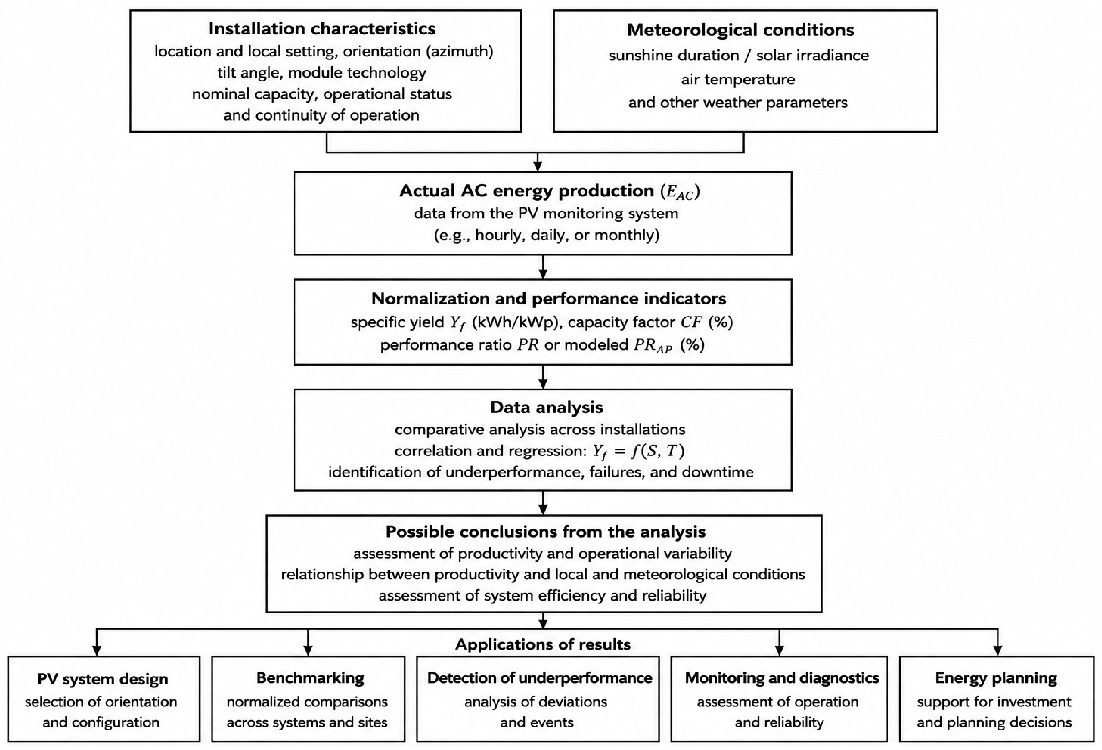
PV-system performance is generally assessed by combining production and meteorological data, normalized indicators, and analyses of reliability and deviations from expected operation. Figure 13 synthesizes these commonly used elements and organizes them into a single analytical sequence that can support a comprehensive assessment of the real-world productivity of PV installations. The diagram presents successive stages of evaluation: from technical and meteorological conditions, through measurement of AC energy production, normalization of results, and data analysis, to assessment of productivity and reliability and applications in design, anomaly detection, monitoring, and energy planning. This framework shows that installation performance should not be assessed solely on the basis of nominal capacity.

5. Conclusions

The four-year analysis of actual operating data from four prosumer photovoltaic microinstallations showed that greater nominal capacity does not guarantee higher energy productivity. The highest mean specific yields were achieved by PV-I and PV-II, each rated at 4.69 kWp and oriented south and southwest, respectively. These values were 1077.7 and 1061.7 kWh/kWp/year, whereas PV-III and PV-IV, each rated at 5.04 kWp, achieved 908.6 and 779.6 kWh/kWp/year, respectively. Relative to the south-facing PV-I system, the mean annual specific yield was 1.5% lower for PV-II (southwest), 15.7% lower for PV-III (southeast), and 27.7% lower for PV-IV (west). The corresponding capacity-factor differences were −0.18, −1.93, and −3.40 percentage points, respectively, while the differences in the model-based PR_AP estimate were +0.3, −11.6, and −16.7 percentage points. These values should be treated as comparative results for the analyzed systems rather than as universal orientation-loss coefficients. The observed differences reflect the combined influence of system geometry, module technology, technical configuration, local operating conditions, and system availability, rather than orientation alone. The results indicate that differences in the actual productivity of microinstallations cannot be explained solely by installed capacity. They may also be related to technical configuration, module orientation and geometry, local operating conditions, and continuity of operation. Among the regional meteorological variables included in the statistical analysis, monthly sunshine duration showed the strongest association with specific yield. Pearson correlation coefficients between sunshine duration and yield ranged from r = 0.830 to 0.983, indicating a strong temporal association between regional sunshine conditions and electricity production. At the same time, the results of individual installations differed despite the use of a common regional meteorological data series. This means that information on regional solar resources alone is insufficient for assessing the operation of a specific system.

The use of normalized indicators, including specific yield, capacity factor, and the model-based PR_AP estimate, confirmed that differences in installation productivity did not result solely from nominal capacity or the adopted irradiation resource. An important element of the analysis was also assessment of the effect of the PV-IV failure in August 2024. Excluding the month of zero production increased the coefficient of determination, R², for the sunshine-duration–yield relationship from 0.689 to 0.812, but PV-IV productivity remained lower than that of the other systems. The failure therefore deepened the observed differences but was not their only cause. In the combined model, excluding the confirmed fault observation increased R² from 0.888 to 0.921. Confirmed fault observations in household PV monitoring data should therefore be retained in the primary analysis and additionally assessed through a sensitivity analysis performed with and without the affected observation. This result emphasizes the importance of regularly reviewing monitoring data and separately accounting for failure events when evaluating installation performance.

From the perspective of SDG 7, the results support the development of affordable, reliable, and locally adapted renewable-energy systems. Planning of household PV in Poland should therefore not rely solely on nominal capacity or regional solar-resource maps. Design and support schemes should additionally consider roof orientation, expected specific yield, local shading conditions, monitoring capability, and the risk of operational downtime. At the regional level, PV-resource assessments should be supplemented with measured performance data from representative household installations and with locally differentiated reference values for specific yield. Such an approach would improve system sizing, facilitate early fault detection, and reduce the risk of overestimating the energy contribution of distributed PV installations.

The results obtained under the conditions of the Sandomierz Basin show that assessment of prosumer microinstallations should be based on a combination of actual operating data, regional meteorological information, and normalized indicators rather than solely on annual energy production or nominal system capacity. The approach used may serve as an example for similar analyses conducted in other regions, provided that their local environmental and technical conditions are taken into account. The scientific value of the study results from combining a four-year observation period, analysis of systems operating within one macroregion, comparison of two pairs of installations with equal capacities, a model-based reference of production to irradiation, and a quantitative assessment of the effect of a failure. This made it possible to assess not only absolute energy production but also the persistence of differences among installations after normalization of the results and inclusion of common meteorological variables.

The real-world operation of microinstallations should be interpreted as the combined effect of technical configuration, the local environment, and continuity of operation. The results may support PV-system design, detection of abnormal operation, and local planning of distributed-energy development, thereby improving the reliability and practical usefulness of household photovoltaics.