Evaluating the Impact of Feature Dimensionality on Price Prediction in the Indian Electricity Market

Abstract

Accurate forecasting of electricity prices is essential for efficient operation and decision-making in deregulated power markets, particularly in the Indian electricity market, characterized by high volatility and dynamic pricing. This study presents a comparative analysis of statistical, machine learning, and deep learning methods for electricity price prediction in the Indian market, with a focus on feature dimensionality. The evaluated models include autoregressive-integrated-moving average, seasonal autoregressive-integrated-moving average, seasonal autoregressive-integrated-moving average with exogenous variables, categorical boosting, random forest, long short-term memory, bidirectional long short-term memory, and a hybrid convolutional neural network-bidirectional long short-term memory model. Historical data available on the Indian Energy Exchange webpage are deployed in this study. The models are analyzed for varying input vector sizes with features that include date, type of day, day of the week, previous day, month, and year market prices. The results indicate improved predictive performance of all model while increasing the input feature dimensionality from five to seven. The results indicate that while increasing the feature size from five to seven increases the prediction accuracy, the gains become marginal beyond seven, emphasizing the importance of feature relevance over feature quantity. From a theoretical perspective, the study highlights the dominance of short-term temporal dependencies in MCP prediction and provides empirical evidence for the point of diminishing returns in feature expansion. From a practical standpoint, the results endorse the choice of computationally efficient and interpretable models for real-world deployment.

1. Introduction

Deregulation is a major development in the energy business all around the world. It is changing how markets and businesses work in many countries [1]. Many developing countries see this transformation as a chance to acquire foreign investment, improve the economy, create jobs, and upgrade energy infrastructure [2]. As part of these changes, current vertically integrated utilities are divided into independent companies for generation (Gencos), transmission (Transcos), and distribution (Discos) to stimulate private investment and competition in the industry. The purpose of these changes in the market is to make the system run better, encourage participants to compete, and improve the operation [3]. Transmission (TSO) and distribution (DSO) system operators play a vital role for coordinated operations between distributed energy resources (DERs) and integrated power systems [4]. Deregulation promotes the integration of many independent power producers using unexpected and dynamic clean energy sources. Privatization increases competition, lowering retail electricity rates. Studies indicate that deregulation makes trade cost-effective [5]. Power system deregulation affects industry market dynamics, regulations, and operations [6]. The transition to the new structure intends to enhance energy market vitality, improve resource allocation, and stimulate efficiency in electricity production and utilization. The market operation can be modeled as a single buyer, bilateral, or poolco [7]. The poolco model [8] is a prominent framework for organizing the spot market in electricity trading, facilitating a transition from traditional industry practices to a competitive market environment [9]. The auction mechanism performed for a prescribed slot involves the determination of the market-clearing price (MCP) by encouraging the submission of bids and offers from the market participants [10]. The market clearing process in the specific slot balances the supply and demand requirements. The dynamic behavior of market players results in varying MCP. Ref. [11] points out the influence of supply and demand dynamics, generation costs, and regulatory policies on energy prices. To maintain a competitive edge, energy industry participants must prioritize the pricing definition [12]. In a deregulated energy sector, market players prioritize profit maximization, often overlooking system-wide benefits. Prediction of electricity price helps consumers plan and schedule their consumption [13]. Meanwhile, the power producers participate in auctions with the aim of being selected as in-merit players and attaining economic benefits from power transactions. This calls for the evolution of accurate price prediction methods in today’s dynamic energy market with many participants. Energy price forecasting [14] is crucial for serving customer demand and enables utilities and customers to collaborate on efficient energy generation and usage, thereby lowering energy costs. Forecasting is found to be more challenging due to the dynamic nature of energy costs, which are impacted by a wide range of factors, including changes in supply and demand, changes in legislation, geopolitical events, and technical breakthroughs [15,16,17].

Researchers have proposed various methods for forecasting electricity prices, tailored to the specific needs of the electricity market. These methods include models based on power usage and related cost information, game theory that analyses the impact of bidders’ strategic behavior, stochastic modeling of various input information, regression, and deep learning models. Ref. [18] focuses on forecasting electricity prices using functional time series analysis, and the method is found to outperform the time series forecasting techniques. In a time series model, a specific sequence of data points is measured over a specific period. Ref. [19] states that the predominant fluctuations in energy price data significantly affect forecast accuracy. Ref. [20] describes a method that uses autoregressive integrated moving average (ARIMA) to analyze historical data and forecast power costs for the next day. To enhance the feature selection process, the model applies a data mining approach for time series analysis. Using time series analysis, Ref. [21] suggests a day-ahead pricing prediction method for a meat plant. Ref. [22] presents an approach to predict the price difference between day-ahead and real-time electricity markets. The authors in [23] posited a price-maker bidding and offering model utilizing mixed integer linear programming to optimize revenue for networked microgrids (NMG) in a pool-based day-ahead electricity market.

Machine learning (ML) models have been proved to interpret future data while detecting similarities and patterns in any available data set. The ML models do not require clear algorithms, as in the case of traditional programming. Refs. [24,25] showed the relevance of ML approaches in forecasting energy costs. Ref. [26] presents a method to improve the accuracy of day-ahead electricity price forecasting using a neural network model enhanced by innovation-based techniques. Ref. [27] proposes a hybrid model that combines wavelet transform and Adam-optimized long short-term memory (LSTM) for accurate energy price prediction. Ref. [28] describes a hybrid model combining metaheuristic algorithms with artificial neural networks (ANNs) for short-term electricity price forecasting. The authors have trained the parameters using vanilla ANN and metaheuristic techniques, including the follow-the-leader ANN (FTL-ANN) algorithm, while proving superior performance. A hybrid architecture based on ANN-PSO (Particle Swarm Optimization) for power price forecasting has been addressed in [29]. Ref. [30] proposes an optimized method combining variational mode decomposition (VMD) and K-Means clustering, enhanced by a novel PSO approach. Ref. [31] introduces a method that creates the prediction range for future prices by using quantile regression to set the upper and lower limits. Additionally, the system uses extreme learning machine (ELM) techniques to analyze intricate price data patterns with parameters optimized using augmented Lagrangian relaxation. Ref. [32] presents a method using Gated Recurrent Units (GRUs) to make price predictions for the day-ahead market. Researchers have developed and carried out performance analysis of time series and ML-based price-prediction models. Ref. [33] attempts to compare the performance of energy price prediction models deploying ARIMA, sequence-to-sequence (Seq2Seq) architecture, and bidirectional long short-term memory (BiLSTM) units to forecast nodal price differences between day-ahead and real-time markets. The summary of prediction models along with the input features and output is presented in Table 1.

The studies summarized in Table 1 show that electricity price, demand, or load prediction use a wide range of approaches, from time series models to ML and deep learning hybrids, reflecting the volatility and complexity of markets’ nature. The time series models easily handle the prediction for datasets with less nonlinearity, while they fail for highly nonlinear datasets. Meanwhile, the ML and deep learning methods incorporate more exogenous factors that improve the forecasting accuracy since they address both demand and supply needs. The Indian electricity market is characterized by high volatility, dynamic pricing across 96 daily intervals, seasonal demand variations, and evolving regulatory frameworks, making it fundamentally different from mature markets. These unique characteristics, combined with limited prior comprehensive study, justified the need for tailored forecasting models and systematic analysis.

1.1. Research Gap

In the context of India’s evolving electricity markets, influenced by deregulation and heightened competition, a notable research gap exists regarding the creation of predictive models specifically designed for the distinct characteristics of the Indian market [34,35]. Despite the existing studies on the Indian power trading platform, which provide important information about market clearance parameters [36,37,38], little research has endeavored to create predictive models tailored to the emerging industry. Prior studies have addressed electricity price forecasting in the Indian power market using data-driven and hybrid approaches. A wavelet-based ANN with embedded PSO for forecasting day-ahead market-clearing price in the Indian energy market is proposed in [29]. Study in [39] presents a data-driven framework using the backpropagation algorithm for predicting spot market prices in the Indian electricity market using historical price data. Ref. [40] employed an ANN-based approach to forecast the market-clearing price using data from the IEX during January 2014 to June 2014.

Table 1. Summary of key studies in input feature vector selection.

Ref. No.	Input Features	Prediction Model	Output	Performance Indices	Remarks
[7]	Hourly electricity demand Hourly electricity price Generation costs Oil price Weather	Model predictive control	Hourly price forward curve	NA	Higher accuracy than heuristic approaches
[12]	Daily minimum temperature Daily maximum temperature Daily average temperature Previous day’s electricity price Previous day’s load data Time slot	Review of time series models, ML models, hybrid models	Short-term and long-term price and load predictions	MAPE	Highlights the limitations of relying on a single performance metric for model evaluation
[13]	Previous coal capacity Previous electricity demand Previous electricity price Previous gas capacity Previous residual load Previous solar and wind energy	Hybrid deep neural network model using CNN and LSTM	Electricity price forecast	MAE RMSE	Proposed a strategic bidding framework for price maker generators CNN–LSTM effectively predicts LMPs in congested markets using aggregated supply curves
[15]	Previous coal capacity Previous electricity demand Previous electricity price Previous gas capacity Previous residual load Previous solar and wind energy Time slot	Time Series Simulation Conditional Generative Adversarial Network (TSS-CGAN)	Electricity price forecast	Continuous ranked Probability score (CRPS) MAE	Offers strong probabilistic forecasting but sensitive to data quality and computationally intensive TSS-CGAN attains lower CRPS (14.29) compared to deep autoregressive (28.49), Prophet (15.65), and temporal fusion transformer (18.51) methods
[18]	Bank holidays Day of the week Previous electricity prices	Functional Time Series Analysis-Functional Autoregressive (FAR)	Electricity price prediction	MAE MAPE RMSE	Supports adaptive lag determination FAR achieves lower MAE (5.16), MAPE (8.99), and RMSE (8.65) and outperforms autoregressive and naive methods
[19]	Previous electricity demand Previous hours’ electricity prices Time slots	ANN based forecasting model	Long term Iberian electricity price prediction	Mean week error (MWE) Forecast Mean Square Error (FMSE)	In the Spanish market, the mean error is about 10%, while in the Californian market, it is nearly 5% during stable periods and around 11% over a three-week horizon without explanatory variables
[20]	Previous day’s electricity market price Previous days’ electricity market prices Time slots	ARIMA	Electricity price prediction for day-ahead Indian electricity market	MAPE	Achieves approximately 10% forecast error in the Spanish market and 5% in the Californian market during stable periods
[23]	Grid constraints Previous days’ energy prices Previous day’s generation capacity Previous day’s demand	Hybrid stochastic robust optimization, MLP, Dantzig-Wolfe decomposition	Optimal bidding and offering strategy for networked microgrids	NA	Accuracy of DRNN with a single SVM and hybrid network has been compared The DRNN model achieves a lower MAPE of 5.63%, outperforming both SVM (35.26%) and hybrid SVM (27.57%) models
[24]	Fuel price Grid constraints Previous hours’ electricity price data Previous hours’ load profile	Deep reinforcement learning (DRL)	Electricity price prediction for market of England	Relative strength index (RSI)	The ARIMA model shows greater RSI fluctuations compared to DRL and indicates that DRL aligns more closely with realized price predictions
[25]	Previous days’ electricity prices Previous days’ demand forecast Fuel prices System load levels Month, day of week	Innovations-based Neural Network (INN)	Electricity price prediction for Spain’s power market	MAPE	Average accuracy improvement is 26%, with an overall MAPE of 6.5%
[28]	Average load of previous day Average price of previous day Electricity price data for the previous day Electricity price from the same hour from the previous day Fuel prices and temperature Holiday/weekend indicator Hour of the day and day of the week Load from the same hour on the previous day Load from the same hour on the same day of previous week Natural gas price	Meta-heuristic Learning Approach: ANN-Follow the Leader (ANN-FTL)	Energy price forecasting	Average error (AE) MAE MAPE RMSE Normalized mean square error (NMSE)	The FTL algorithm outperforms cuckoo search, particle swarm, and fruit fly optimization in enhancing ANN accuracy for energy price forecasting The paper presents the performance metrics AE, MAE, MAPE, RMSE, and NMSE, which are 0.20, 6.67, 8.18, 10.67, and 0.15 respectively
[29]	Previous hours’ market-clearing price Previous hours’ demand data Hourly purchase bid	Sequential Wavelet-ANN With Embedded ANN-PSO	Energy price prediction	Error variance (EV) MAPE NMSE	Wavelet-based ANN–ANN-PSO delivers superior performance metrics EV of 8.3911 × 101, MAPE of 9.2523, and NMSE of 2.5696 × 10−8
[30]	Historical price data Energy demand levels Energy generation data Hourly temperature and humidity	Signal decomposition and clustering techniques	Energy price prediction	MAE MAPE MSE	The Decomposition–clustering approach achieves the lowest prediction error MAE, MSE, and MAPE are 0.018, 0.0007 and 6.15% respectively
[31]	Electricity price data Time slot	Novel data mining approach for electricity price forecast	Electricity price forecasting	Average coverage error (ACE)	ACE value for the model is 1.59%, which is smaller than the ACE value of the previous method (2.03%)
[32]	Trend of spot prices for West Texas Intermediate (WTI) crude oil Trend of spot prices for Brent crude oil Trend of spot prices for reformulated gasoline blend stock for oxygenate blending	Hybrid SW GRU with EMD	Energy price forecasting	MSE MAPE Symmetric mean absolute percent error (SMAPE) Theil inequality coefficient (TIC)	Enables probabilistic forecasting with optimized prediction intervals for improved reliability MAPE, RMSE, SMAPE, and TIC as 1.0678, 0.97, 0.0107 and 0.0061
[33]	Capacity of generation resources Transmission constraints Energy demand	Extended poolco model	Spot pricing prediction of electricity	Not specified	Market maker system for P2P electricity trading mitigating extreme fluctuations
[41]	Time series data of Wolf’s sunspot data, the Canadian data and the IBM stock price data	Hybrid model combining ARIMA with ANN	Stock price prediction	Mean absolute Deviation (MAD) MSE MAPE	MSE, MAD, and MAPE values are 0.103524, 0.018625, and 3.589712%, respectively
[42]	Previous hours’ electricity prices	ARIMA model approach and expert modeler	Electricity price forecasting	MAPE	MAPE and MaxAPE for the model are 3.55% and 33.1%
[43]	Previous load data from the Yunnan power grid Seasonal indices	SARIMA	Load forecasting	MAPE	The SARIMA model is a more viable and effective tool for medium- and long-term load forecasting than HOLT_WINTER, LSTM, and ARIMA The MAPE obtained for the model is 6.05%
[44]	Previous electricity price Previous electricity demand Energy generated from wind Energy generated from solar Energy generated from gas Energy generated from coal Energy generated from nuclear stations Energy generated from hydroelectric power stations Energy generated from biomass Temperature	SARIMAX	Electricity price forecasting	RMSE	The SARIMAX model is compared with the SARIMA model The RMSE values obtained for the SARIMAX model for spring, summer, autumn, and all seasons are 8.93, 9.36, 7.75, and 8.5, respectively
[45]	Carbon dioxide (CO2) coupons Previous 5 years’ electricity price data from EU energy market Weather conditions Oil prices	ML approach with local searcher genetic programming (LSGP)	Electricity price forecasting	MAE	Claims lower MAE compared to models trained using Geometric Semantic Genetic Programming
[46]	Electricity spot price data of the Nord pool market Weather data	Bi-LSTM and CatBoost	Electricity price forecasting	MAPE RMSE MAE Training and testing time	Achieves the lowest MAPE (5.142), RMSE (36.885), and MAE (24.485), with training and testing times of 83.434 s and 3.030 s, respectively
[47]	Day of the week Season Electricity price data	LSTM optimized with Adam optimizer and integrated with wavelet transforms (WT-Adam- LSTM)	Electricity price forecasting for the Australian and French market	RMSE MAE MAPE	MAPE of 1.5, RMSE of 0.62, and MAE of 0.62
[48]	Actual power generation Areal meteorological forecasts Calendar holidays Previous year’s electricity prices from the Japanese market Land area pixel Metrological data Weather variables	CNN–LSTM model	Electricity price forecasting	RMSE MAE R2	RMSE, MAE, and R2 are 2.630, 1.936, and 0.787 respectively

Table 1. Summary of key studies in input feature vector selection.

Ref. No.	Input Features	Prediction Model	Output	Performance Indices	Remarks
[7]	Hourly electricity demand Hourly electricity price Generation costs Oil price Weather	Model predictive control	Hourly price forward curve	NA	Higher accuracy than heuristic approaches
[12]	Daily minimum temperature Daily maximum temperature Daily average temperature Previous day’s electricity price Previous day’s load data Time slot	Review of time series models, ML models, hybrid models	Short-term and long-term price and load predictions	MAPE	Highlights the limitations of relying on a single performance metric for model evaluation
[13]	Previous coal capacity Previous electricity demand Previous electricity price Previous gas capacity Previous residual load Previous solar and wind energy	Hybrid deep neural network model using CNN and LSTM	Electricity price forecast	MAE RMSE	Proposed a strategic bidding framework for price maker generators CNN–LSTM effectively predicts LMPs in congested markets using aggregated supply curves
[15]	Previous coal capacity Previous electricity demand Previous electricity price Previous gas capacity Previous residual load Previous solar and wind energy Time slot	Time Series Simulation Conditional Generative Adversarial Network (TSS-CGAN)	Electricity price forecast	Continuous ranked Probability score (CRPS) MAE	Offers strong probabilistic forecasting but sensitive to data quality and computationally intensive TSS-CGAN attains lower CRPS (14.29) compared to deep autoregressive (28.49), Prophet (15.65), and temporal fusion transformer (18.51) methods
[18]	Bank holidays Day of the week Previous electricity prices	Functional Time Series Analysis-Functional Autoregressive (FAR)	Electricity price prediction	MAE MAPE RMSE	Supports adaptive lag determination FAR achieves lower MAE (5.16), MAPE (8.99), and RMSE (8.65) and outperforms autoregressive and naive methods
[19]	Previous electricity demand Previous hours’ electricity prices Time slots	ANN based forecasting model	Long term Iberian electricity price prediction	Mean week error (MWE) Forecast Mean Square Error (FMSE)	In the Spanish market, the mean error is about 10%, while in the Californian market, it is nearly 5% during stable periods and around 11% over a three-week horizon without explanatory variables
[20]	Previous day’s electricity market price Previous days’ electricity market prices Time slots	ARIMA	Electricity price prediction for day-ahead Indian electricity market	MAPE	Achieves approximately 10% forecast error in the Spanish market and 5% in the Californian market during stable periods
[23]	Grid constraints Previous days’ energy prices Previous day’s generation capacity Previous day’s demand	Hybrid stochastic robust optimization, MLP, Dantzig-Wolfe decomposition	Optimal bidding and offering strategy for networked microgrids	NA	Accuracy of DRNN with a single SVM and hybrid network has been compared The DRNN model achieves a lower MAPE of 5.63%, outperforming both SVM (35.26%) and hybrid SVM (27.57%) models
[24]	Fuel price Grid constraints Previous hours’ electricity price data Previous hours’ load profile	Deep reinforcement learning (DRL)	Electricity price prediction for market of England	Relative strength index (RSI)	The ARIMA model shows greater RSI fluctuations compared to DRL and indicates that DRL aligns more closely with realized price predictions
[25]	Previous days’ electricity prices Previous days’ demand forecast Fuel prices System load levels Month, day of week	Innovations-based Neural Network (INN)	Electricity price prediction for Spain’s power market	MAPE	Average accuracy improvement is 26%, with an overall MAPE of 6.5%
[28]	Average load of previous day Average price of previous day Electricity price data for the previous day Electricity price from the same hour from the previous day Fuel prices and temperature Holiday/weekend indicator Hour of the day and day of the week Load from the same hour on the previous day Load from the same hour on the same day of previous week Natural gas price	Meta-heuristic Learning Approach: ANN-Follow the Leader (ANN-FTL)	Energy price forecasting	Average error (AE) MAE MAPE RMSE Normalized mean square error (NMSE)	The FTL algorithm outperforms cuckoo search, particle swarm, and fruit fly optimization in enhancing ANN accuracy for energy price forecasting The paper presents the performance metrics AE, MAE, MAPE, RMSE, and NMSE, which are 0.20, 6.67, 8.18, 10.67, and 0.15 respectively
[29]	Previous hours’ market-clearing price Previous hours’ demand data Hourly purchase bid	Sequential Wavelet-ANN With Embedded ANN-PSO	Energy price prediction	Error variance (EV) MAPE NMSE	Wavelet-based ANN–ANN-PSO delivers superior performance metrics EV of 8.3911 × 101, MAPE of 9.2523, and NMSE of 2.5696 × 10−8
[30]	Historical price data Energy demand levels Energy generation data Hourly temperature and humidity	Signal decomposition and clustering techniques	Energy price prediction	MAE MAPE MSE	The Decomposition–clustering approach achieves the lowest prediction error MAE, MSE, and MAPE are 0.018, 0.0007 and 6.15% respectively
[31]	Electricity price data Time slot	Novel data mining approach for electricity price forecast	Electricity price forecasting	Average coverage error (ACE)	ACE value for the model is 1.59%, which is smaller than the ACE value of the previous method (2.03%)
[32]	Trend of spot prices for West Texas Intermediate (WTI) crude oil Trend of spot prices for Brent crude oil Trend of spot prices for reformulated gasoline blend stock for oxygenate blending	Hybrid SW GRU with EMD	Energy price forecasting	MSE MAPE Symmetric mean absolute percent error (SMAPE) Theil inequality coefficient (TIC)	Enables probabilistic forecasting with optimized prediction intervals for improved reliability MAPE, RMSE, SMAPE, and TIC as 1.0678, 0.97, 0.0107 and 0.0061
[33]	Capacity of generation resources Transmission constraints Energy demand	Extended poolco model	Spot pricing prediction of electricity	Not specified	Market maker system for P2P electricity trading mitigating extreme fluctuations
[41]	Time series data of Wolf’s sunspot data, the Canadian data and the IBM stock price data	Hybrid model combining ARIMA with ANN	Stock price prediction	Mean absolute Deviation (MAD) MSE MAPE	MSE, MAD, and MAPE values are 0.103524, 0.018625, and 3.589712%, respectively
[42]	Previous hours’ electricity prices	ARIMA model approach and expert modeler	Electricity price forecasting	MAPE	MAPE and MaxAPE for the model are 3.55% and 33.1%
[43]	Previous load data from the Yunnan power grid Seasonal indices	SARIMA	Load forecasting	MAPE	The SARIMA model is a more viable and effective tool for medium- and long-term load forecasting than HOLT_WINTER, LSTM, and ARIMA The MAPE obtained for the model is 6.05%
[44]	Previous electricity price Previous electricity demand Energy generated from wind Energy generated from solar Energy generated from gas Energy generated from coal Energy generated from nuclear stations Energy generated from hydroelectric power stations Energy generated from biomass Temperature	SARIMAX	Electricity price forecasting	RMSE	The SARIMAX model is compared with the SARIMA model The RMSE values obtained for the SARIMAX model for spring, summer, autumn, and all seasons are 8.93, 9.36, 7.75, and 8.5, respectively
[45]	Carbon dioxide (CO2) coupons Previous 5 years’ electricity price data from EU energy market Weather conditions Oil prices	ML approach with local searcher genetic programming (LSGP)	Electricity price forecasting	MAE	Claims lower MAE compared to models trained using Geometric Semantic Genetic Programming
[46]	Electricity spot price data of the Nord pool market Weather data	Bi-LSTM and CatBoost	Electricity price forecasting	MAPE RMSE MAE Training and testing time	Achieves the lowest MAPE (5.142), RMSE (36.885), and MAE (24.485), with training and testing times of 83.434 s and 3.030 s, respectively
[47]	Day of the week Season Electricity price data	LSTM optimized with Adam optimizer and integrated with wavelet transforms (WT-Adam- LSTM)	Electricity price forecasting for the Australian and French market	RMSE MAE MAPE	MAPE of 1.5, RMSE of 0.62, and MAE of 0.62
[48]	Actual power generation Areal meteorological forecasts Calendar holidays Previous year’s electricity prices from the Japanese market Land area pixel Metrological data Weather variables	CNN–LSTM model	Electricity price forecasting	RMSE MAE R2	RMSE, MAE, and R2 are 2.630, 1.936, and 0.787 respectively

The model incorporates price one day ago, change in demand, price one week ago, forecasted demand, price two weeks ago, a time slot of the day, price three weeks ago, day of the week, and price four weeks ago as input parameters. Ref. [49] presents a method by employing an XGBoost model to indicate the price at which electricity is transacted, using IEX input data from 2019 to 2024. Ref. [50] proposes and compares models based on LSTM and Gated Recurrent Unit (GRU) to predict the MCP for the Indian market, deploying the data available in IEX. Ref. [51] investigates the effectiveness of advanced forecasting models for time series data such as long short-term memory (LSTM), SARIMA, XGBoost, and Facebook Prophet in predicting MCP for the dynamic Indian electricity market using monthly, yearly, and weekly IEX data. Although these studies improve the understanding of price prediction in the Indian electricity market, the authors evaluate each proposed method independently without comparing the performance of the model with alternate forecasting techniques used in the same market. The present study addresses this limitation by conducting a systematic and thorough comparative performance evaluation of multiple forecasting methodologies.

The efficacy of forecasting models is heavily reliant upon the quality of data, feature selection, and the methods employed for preprocessing. The existing literature inadequately addresses the essential problem of formulating optimal input feature vectors that can significantly impact model accuracy. Many studies fail to incorporate dynamic elements such as market-specific indicators including day type, day of the week, holidays, and special events, which affects the accurate prediction of MCP. Although most models predominantly depend on fundamental temporal information (date, time, and historic MCP), the incorporation of additional features like the day of the week, type of day (business day or weekend), the previous month’s same day, and the same day of the same month in the previous year also significantly improves forecast accuracy.

The depth of the input feature set plays an important role in model performance. Adding more relevant input features helps models to capture more complex temporal dependencies and nonlinear linkages. This reduces residual errors and improves overall forecasting accuracy. Nonetheless, the influence of feature depth on prediction accuracy remains underexplored, particularly in the context of electricity price forecasting. Choosing the most outstanding predictive model along with a well-formulated input feature vector helps to close the research gap and assists the market participants in refining bidding strategies and consumption schedules within India’s dynamic market environment. In the context of the Indian electricity market, the prediction models face challenges due to high price volatility and strong short-term dependencies. In short, the existing studies in the Indian electricity market largely focus on individual model development without systematic comparison, while the impact of feature selection and dimensionality on prediction performance remains insufficiently explored, particularly for market-specific features, emphasizing the necessity of a comprehensive and integrated analysis.

1.2. Highlghts of the Article

Based on the identified research gap, the highlights of the paper are mentioned below:

The paper aims to develop the best model to predict the Indian market electricity price by performing the following:

• Data collection for the period between 1 January 2017 and 31 December 2021 from the Indian Energy Exchange (IEX).
• Perform preprocessing of the collected data set, including min–max scaling.
• Prepare the input feature vector with sizes of five, six, and seven that comprise date, type of day, day of the week, and historic MCP and split the same into train and test subsets.
• Develop ARIMA, SARIMA, SARIMAX, CatBoost, random forest (RF), LSTM, BiLSTM, and CNN-BiLSTM models for MCP prediction employing the dataset created in 3.
• Carry out performance evaluation of the considered models with respect to variation in input feature set through the analysis of the performance indices, including root mean square error (RMSE), mean absolute error (MAE), R² score, and mean absolute percentage error (MAPE). The best model with enhanced performance is finally suggested for future applications.

The novelty of the article lies in providing empirical evidence on feature relevance and model behavior under varying feature dimensions rather than proposing complex feature engineering techniques. The approach offers practical insights for designing efficient forecast models with minimal feature sets.

1.3. Contribution of the Article

The key contributions of the article are as follows:

• A systematic evaluation of statistical, ML, and deep learning models for MCP prediction in the Indian electricity market using real-time IEX market data.
• A feature dimensionality analysis demonstrates the impact of increasing feature size from five to seven and identifying the point of diminishing returns.
• An interpretability-driven analysis using feature importance, revealing the dominance of short-term temporal dependencies over long-term seasonal features.
• A market-specific insight for the Indian electricity market showing that conventional features behave differently due to high volatility and short-term price dependency.
• Development of a practical and computationally efficient framework suitable for the Indian electricity market.

The paper is organized as follows: Section 2 delineates the power trading in a deregulated environment along with different price forecasting models for the Indian electricity market. Section 3 presents in detail the development of different time series and data-driven models, performance evaluation, and the selection of the best prediction model. Section 4 concludes the findings.

2. Power Trading in a Deregulated Environment

The goal of electricity market operation is to ensure an efficient, reliable, and competitive supply of electricity. This article considers the operation of a day-ahead poolco market that allows various entities, including traditional utilities, independent power producers, and retailers, to compete for the supply and procurement of electricity. The offers and bids are sent to the wholesale market for each day, and the in-merit participants are chosen by the market clearing procedure based on the offer and bid. Prices [52] are determined by the highest accepted bid among generators dispatched to meet the market power. The in-merit players are provided with settlement information that includes MCP and market clearing volume (MCV). The dynamic nature of players results in varying MCP for each slot in a day.

2.1. Indian Market-Clearing Price Forecasting Models

In competitive markets, power sellers are required to be capable of predicting prices [53]. Accurate predictions of electricity prices help utility companies, grid operators, and market actors to optimize their generation schedules, prepare consumption against price volatility [54], and make investment decisions. Furthermore, a reliable energy price forecast enhances the balance between energy supply and demand, which makes the system less unstable as more renewable energy sources are added. Furthermore, accurate prediction of energy prices can aid policymakers in designing effective energy policies and regulations. This calls for an effective price prediction model. The study considers time series models including ARIMA, SARIMA, and SARIMAX and ML models like RF, CatBoost, LSTM, BiLSTM, and CNN-BiLSTM to perform price predictions.

The ARIMA model [41] is widely used for univariate forecasting [42]. It combines autoregressive (AR), integrated (I), and moving-average (MA) components, denoted as ARIMA (p, d, q). The model development typically follows the steps of testing stationarity, differencing if needed, identifying model order, estimating parameters, and finally performing diagnostic checks and forecasting. The SARIMA time series forecasting model is based on the ARIMA model and takes into account seasonal changes [55]. The non-seasonal elements are denoted as (p, d, q), whereas the seasonal components are represented by (P, D, Q). SARIMA is beneficial for investigating and predicting patterns that alter over time in a cyclic way. SARIMA is a flexible model to look at time series data because it can handle both long-term and short-term changes [43]. The SARIMAX is an improved model for time series prediction. The approach is highly effective for anticipating MCP in electricity markets because it takes into account both seasonality and other external factors influencing energy prices [44]. These statistical time series models are simple and computationally efficient, while the advanced model incorporates exogeneous variables, improving realism. However, the model performance degrades under high price spikes and volatility.

Researchers extensively use ML techniques in energy price prediction because they can learn complex patterns from large historical market datasets. These models offer more reliable, accurate, and timely price forecasts, aiding investors and traders in making prudent decisions [45]. The paper considers modeling RF, CatBoost, LSTM, BiLSTM, and CNN-BiLSTM networks to predict the MCP in the deregulated Indian electricity market. The RF algorithm is a well-known tree-based ensemble learning method that uses outputs from several decision trees [56]. Each tree is trained on a random subset of data and features, which reduces overfitting and improves robustness. The CatBoost algorithm is a supervised ML algorithm that employs gradient boosting to build an ensemble of decision trees [46]. The algorithm begins with a baseline prediction and adds trees iteratively, with each tree aiming to lower the errors from the predecessors. It works effectively for tasks with categorical features and has gained popularity because of its feature handling effectiveness without extensive preprocessing and integration to handle diverse data types. These models have less restrictive assumptions compared to statistical models and hence are suitable to capture nonlinear relationships and feature interactions. However, researchers must address the sensitivity of these models to feature selection and data quality.

Deep learning has emerged as a powerful approach for prediction in complex, nonlinear, and highly dynamic environments. The LSTM [47] model has proved its ability to handle the long-term dependency problem by using gated memory cells that retain information over extended sequences. Due to this capability, it is highly effective for energy price prediction. The BiLSTM architecture extends the processing sequences in both forward and backward directions, allowing it to capture more temporal patterns and context than a unidirectional LSTM. This makes the model well-suited for sequence-to-sequence applications [57,58]. The CNN–BiLSTM is a hybrid model that further enhances predictive performance by combining CNN’s ability to extract local spatial features along with BiLSTM’s strength in modeling long-range dependencies. This integration helps capture both short-term and long-term temporal structures in complex sequential data, improving accuracy in energy price forecasting [58]. Meanwhile, these models are computationally complex and require high training time.

2.2. Data Collection, Preprocessing and Model Evaluation

Data gathering is one of the most important steps in implementing the prediction model. This stage involves gathering current and historical data. Data collection is a fundamental and critical step in the development of accurate and reliable models for energy price prediction. The data is collected from IEX, which is made available to the public. IEX serves as a marketplace for buyers and sellers, including power generators, Discos, and consumers. The buyers and sellers can engage in the purchase and sale of electricity through an online bidding process. IEX operates under the regulatory framework of the Central Electricity Regulatory Commission (CERC) and complies with the guidelines and regulations set by the relevant authorities. IEX has a strong network of more than 7300 participants across five union territories and 29 states, including over 1800 renewable energy producers, 55 Discos, and 600 traditional power generators. The data includes date, slot number, and the corresponding MCP. In this case, the input features include the date and slot number, while the response is the MCP. Existing literature suggests escalation of the feature count to guarantee better model prediction. This paper considers time-tagged energy price details to develop the time series-based prediction model. However, the ML models are provided with features like day of the week and the MCP of the previous months in addition to date and slot number. In an LSTM model, it is important to choose the right window size to collect the trends in the datasets and temporal patterns. This approach balances the short-term changes with long-term patterns to guarantee accurate and dependable price forecasting.

A raw dataset consists of missing entries, errors, outliers, and inconsistencies that make the prediction model less accurate. Data cleaning to remove missing values and scaling to maintain data integrity, feature engineering to capture relevant information, handling the categorical data, and temporal aggregation to capture temporal patterns are all part of data preprocessing. The input dataset is subjected to min–max scaling as per Equation (1).

Scaling the numeric values to a standard range between 0 and 1 helps to mitigate issues related to differing magnitudes of features. The study considers features like date, day of the week, type of day, MCP of previous day, MCP of the same day on the previous week, MCP of the same day in the previous month, and MCP of the same day in the same month of previous year. The various features included in the study are listed in

Table 2. Feature vector details.

Feature Set	Features Included	Remarks
5-feature set	Date Day of the week Type of day MCP of previous day MCP of previous week same day	Captures calendar effects, short-term price dependency, and weekly price behavior
6-feature set	Date Day of the week Type of day MCP of previous day MCP of previous week same day Previous month’s same day MCP	Extends the 5-feature set by incorporating monthly temporal dependency
7-feature set	Date Day of the week Type of day MCP of previous day MCP of previous week same day Previous month’s same-day MCP Previous year’s same-date MCP	Extends the 6-feature set by incorporating long-term seasonal or yearly price dependency

. While weather parameters are not explicitly modeled, their impact is implicitly reflected in historical MCP values, as electricity prices are driven by demand patterns influenced by seasonal and climatic conditions. Therefore, features such as the MCP of the same day in the previous month and the MCP of the same day on the same month of the previous year act as proxies for underlying weather-driven demand variations, enabling the model to capture seasonal price behavior without direct weather input. Feature importance analysis is performed for optimal selection of input features. Prior to model training, the preprocessed dataset is split into training and testing subsets using a 70:30 ratio to enable unbiased performance assessment. To ensure robust and error-free validation, the data is partitioned into multiple folds for cross-validation. Since the MCP data are inherently sequential, a walk-forward validation strategy is employed to preserve the temporal order of the observations, thus eliminating temporal leakage. The accuracy metrics provide a complementary perspective, with RMSE penalizing large errors and MAPE offering scale-independent evaluation. These evaluation criteria are consistent with prior studies (Table 1) in electricity price forecasting.

$$x^{\prime }=\mathrm{ }{\displaystyle \frac{x\mathrm{ }-\mathrm{ }{x}_{min}}{x_{max}\mathrm{ }-\mathrm{ }{x}_{min}}}$$

(1)

3. Results and Discussion

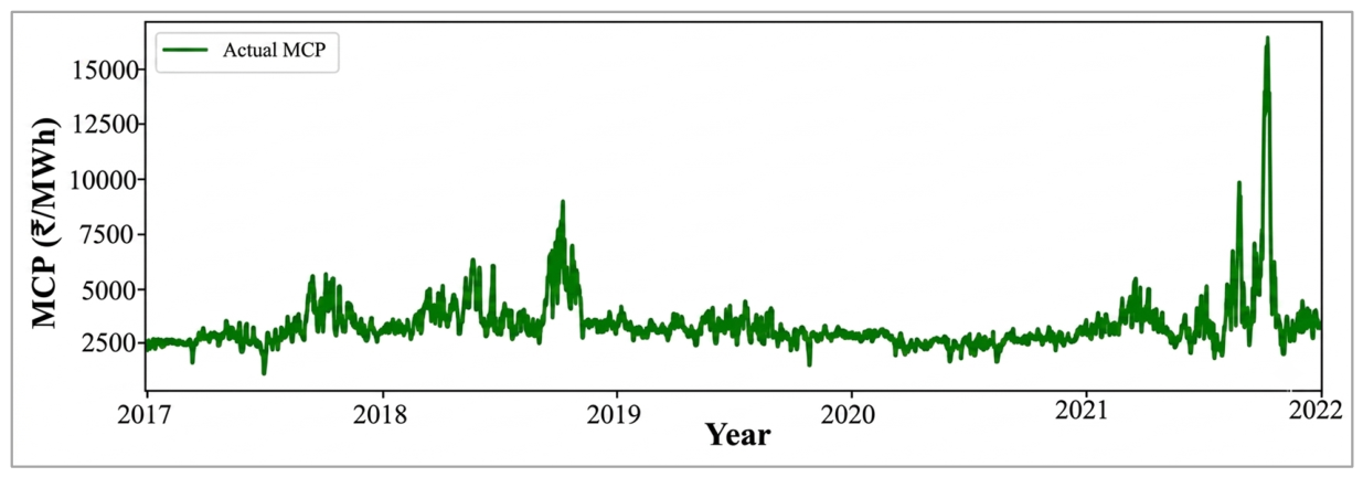
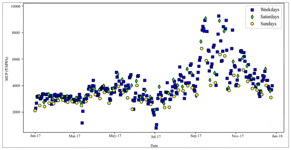
The analysis of diverse methodologies for energy price forecasting demonstrates considerable improvements in accuracy and reliability through the integration of different techniques. This article focuses on the selection of a suitable MCP prediction model for the Indian electricity market. This section covers the modeling and performance evaluation of ARIMA, SARIMA, SARIMAX, CatBoost, RF, LSTM, BiLSTM, and CNN-BiLSTM. The development of data-driven models calls for suitable historical data related to the Indian day–ahead electricity market. As mentioned in Section 2.2, the required data are collected from the IEX webpage for the period between 1st January 2017 and 31st December 2021. The input data sample is illustrated in Figure 1.

Figure 1 illustrates the input sample dataset from 1st January 2017 to 31st December 2021. The preprocessing of data, as mentioned in Section 2.2, consists of data cleaning, normalization, and scaling features. The scaling and normalization bring all features to a similar scale, while preventing the dominance of certain variables. This facilitates better convergence and model performance. The preprocessed data is categorized into train and test categories in the ratio of 70:30. It is now required to train the model, employing 70% of preprocessed data. A systematic strategy has been employed to build and validate prediction models. The best time series model is selected based on the minimum AIC value. The ML models’ hyperparameters are selected through cross-validation while dividing the input data into several folds. A fold denotes a distinct partition of the dataset allocated for training and validation. Using several folds allows an extensive evaluation across diverse temporal segments, which ensures reliable performance. Each model is trained with a segment in each fold, and hyperparameters are adjusted using the right selection criteria. The chosen configuration is then tested on the validation segment, and performance metrics are calculated. The MCP prediction under three input feature configurations, five, six, and seven, using different models has been evaluated. Final model selection relies on cross-validated forecast accuracy instead of a single criterion, hence ensuring robust generalization.

3.1. Time Series Model

This section explains the development of the ARIMA, SARIMA, and SARIMAX models that are trained based on the historical data to predict the Indian MCP.

3.1.1. ARIMA Model

This section focuses on the design and performance evaluation of the ARIMA model. The trained data set that includes 1050 observations is fed to the ARIMA model. Different combinations of (p, d, q) values are deployed to evaluate the ARIMA model. The sample p, d, q orders corresponding to different AIC are tabulated in

Table 3. Sample AIC for different p, d, q of the ARIMA Model.

Rank	Order (p, d, q)	AIC
1	2, 1, 1	−7593.772
2	1, 2, 1	−7583.509
3	1, 0, 0	−7576.673
4	1, 0, 1	−7574.753
5	0, 1, 1	−7572.845

.

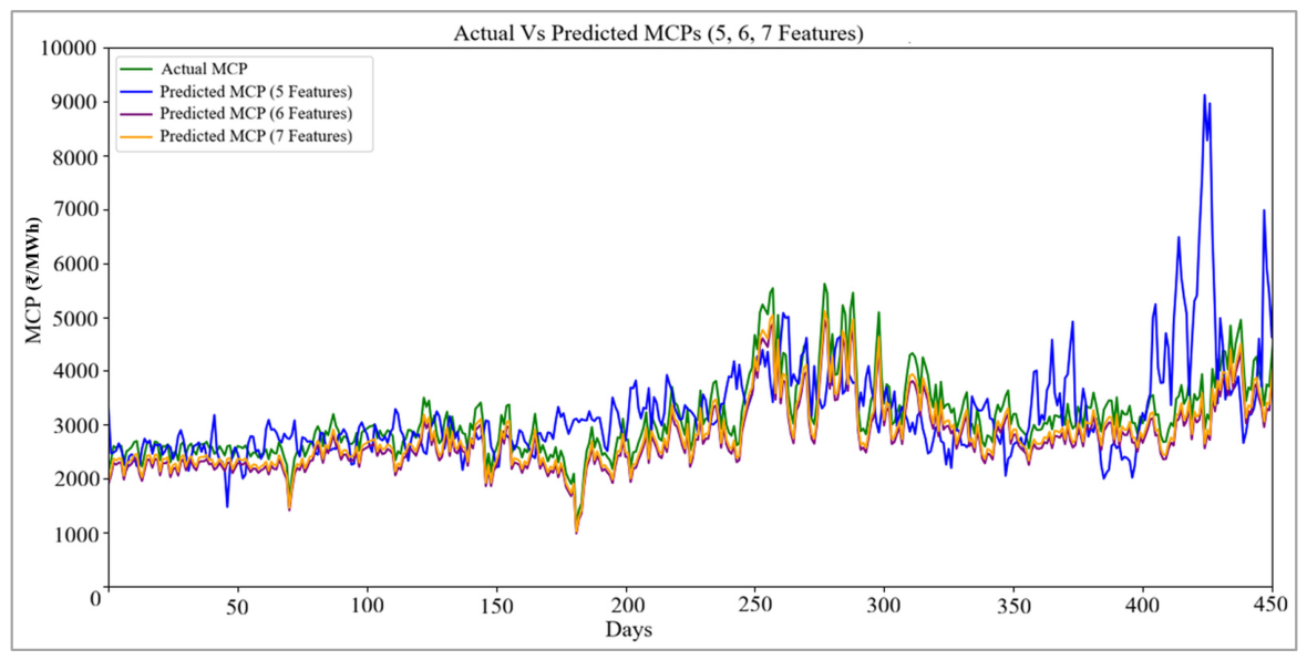
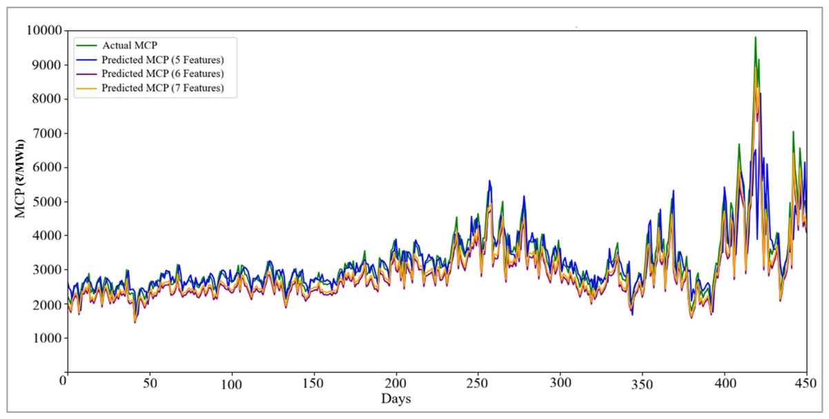
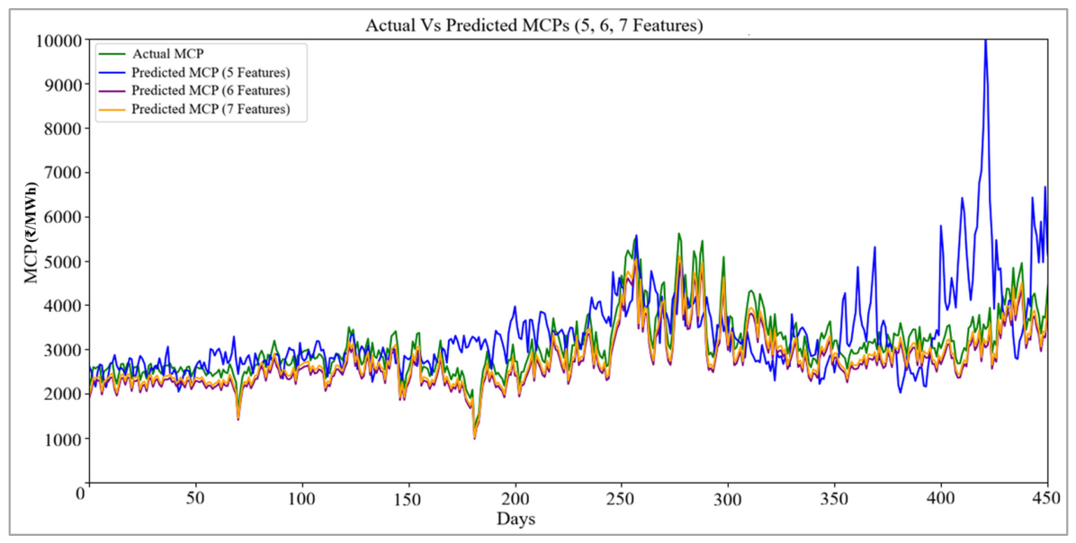
From Table 3, the minimum observed AIC value for the ARIMA model is −7593.772, and the p, d, q values corresponding to the minimum AIC are (2, 1, 1) with Rank of 1. The ARIMA (2, 1, 1) is provided with 450 test data points for the period between 1st July 2020 and 31st December 2021 to evaluate the performance of the model. The time series forecasting typically relies on features such as date, time slots, and MCP. In this study, an enhanced feature set by incorporating additional temporal and contextual variables such as day of the week, type of day, MCP of the previous day, same weekday from the previous week, same day from the previous month, and same date from the previous year is employed [59]. The performance evaluation is done using MAE, RMSE, MAPE, and R² with five, six, and seven input feature sets. When using five input features, ARIMA records the performance indices as ₹293.79/MWh, ₹472.83/MWh, 13.06%, and 0.863 for MAE, RMSE, MAPE, and R² respectively. When the input feature set is expanded to six, the model’s MAE is ₹296.86/MWh, RMSE is ₹483.54/MWh, MAPE is 12.975%, and R² is 0.856. With seven input features, the ARIMA model achieves an MAE of ₹299.45/MWh, an RMSE of ₹497.31/MWh, a MAPE of 13.467%, and R² of 0.869. This trend reflects a significant reduction in the model’s forecasting ability as the number of features increases. The model is then deployed to predict the MCP. The predicted and the actual MCPs for each day during the period from 1 July 2020 to 31 December 2021 for a dataset of 450 days are shown in Figure 2.

Figure 2 reveals the accuracy of the model’s performance in predicting Indian MCP values. The model successfully tracks trends, but minor discrepancies occur at multiple time stamps during overshoots and undershoots. In addition, the model fails to provide a satisfactory prediction during overshoot for the days from 80 to 90, 115 to 130, 140 to 150, 250 to 260, and 300 to 350. Similarly, the MCP prediction accuracy for undershoots is poor for the days 370 to 390 and 410 to 415.

3.1.2. SARIMA Model

This section covers the modeling and performance analysis of the SARIMA model. Different combinations of (p, d, q) and seasonal parameters are provided to determine the best SARIMA model. The pre-processed 70% of input data is fed into the model. The AIC approach is employed to determine the seasonal and non-seasonal parameters of this model. The sample AIC values with the corresponding order are shown in

Table 4. Sample AIC for different p, d, q and P, D, Q of the SARIMA Model.

Rank	Order (p, d, q) (P, D, Q)	AIC
1	(1, 0, 1) (1, 0, 2)	−7600.414
2	(2, 1, 3) (4, 1, 4)	−7568.868
3	(0, 1, 3) (3, 1, 4)	−7564.636
4	(3, 2, 1) (1, 1, 3)	−7562.653
5	(3, 2, 1) (1, 1, 3)	−7557.459

.

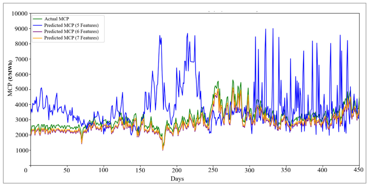
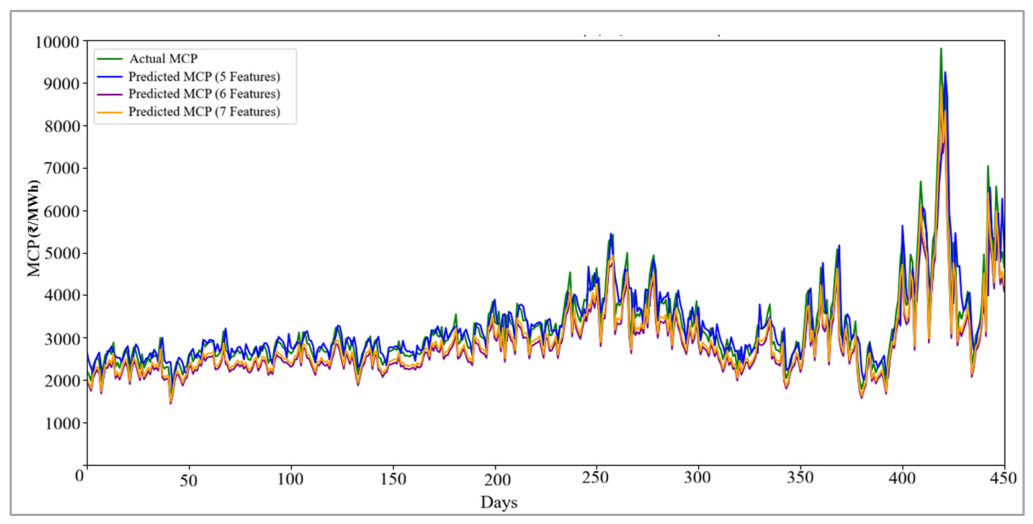
From Table 4, the minimum observed AIC value of the SARIMA model is −7600.414. The p, d, q and the seasonal parameters P, D, Q corresponding to the minimum AIC are (1, 0, 1) and (1, 0, 2), respectively. The trained SARIMA (1, 0, 1), (1, 0, 2) model is now fed with a 30% test subset to evaluate the performance. For the data during the period from 1st July 2020 to 31st December 2021, the SARIMA model demonstrates a consistent enhancement in forecasting performance with an increase in the number of input features. With five input features, the model records an MAE of ₹367.24/MWh, an RMSE of ₹642.68/MWh, a MAPE of 14.329%, and R² of 0.870, indicating a moderate accuracy. When the input set is expanded to six features, SARIMA shows enhanced performance with a reduced MAE of ₹301.45/MWh, RMSE of ₹581.47/MWh, MAPE of 14.01%, and R² value of 0.889. When the input feature changes to seven, the model attains an MAE of ₹293.79/MWh, an RMSE of ₹580.53/MWh, a MAPE of 13.82%, and R² of 0.883. Figure 3 displays the predicted and actual values.

Figure 3 clearly shows that SARIMA is able to successfully follow the trend by increasing the input features from five to seven for training the model. In addition, the SARIMA model fails to anticipate the overshoot for the days 130 to 145, 155 to 165, 260 to 270, 280 to 285, 300, and 340. It also failed to predict the MCP value for undershoots for 15 to 20, 290 to 300, and 362.

3.1.3. SARIMAX Model

This section focuses on the design and performance evaluation of the SARIMAX model. The preconditioned train dataset is fed to the SARIMAX model. The considered model is associated with both seasonal and non-seasonal parameters with exogenous factors. The exogenous factor corresponds to the seasonal frequency (s). The seasonal parameters with exogenous factors (P, D, Q, s) capture the cyclic patterns occurring over fixed intervals, such as days, months, or years.

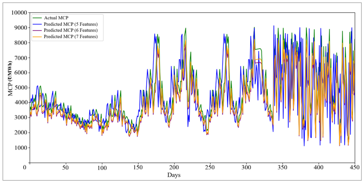
On the other hand, the non-seasonal parameters (p, d, q) address the trend and random variations in the time series. They capture the autocorrelation, differencing, and moving average effects within the data. With the training data, the model is able to produce seasonal and non-seasonal orders corresponding to different AIC values. A sample set of different performance indices against the best five orders is given in

Table 5. Sample AIC for different p, d, q and P, D, Q, S of the SARIMAX model.

Rank	Order (p, d, q)	Seasonal Order (P, D, Q, S)	AIC
1	1, 1, 2	1, 1, 1, 7	−7704.775
2	3, 1, 2	1, 1, 1, 7	−7524.796
3	2, 1, 3	1, 1, 2, 12	−7493.379
4	2, 1, 1	1, 1, 1, 12	−7444.845
5	3, 1, 3	2, 1, 3, 7	−7298.698

. The lower AIC value corresponds to the best-fit model and is found to be −7704.775. Table 5 shows the minimum AIC value corresponding to (p, d, q), (P, D, Q, S) as (1, 1, 2), (1, 1, 1, 7). The SARIMAX (1, 1, 2) (1, 1, 1, 7) model is now evaluated for the performance metrics MAE, RMSE, MAPE, and R² for five, six, and seven input features. The predicted values obtained from the SARIMAX model show strong alignment with actual MCP trends. With five input features, performance indices are observed to be 545.57 (₹/MWh), 824.17 (₹/MWh), 12.39%, and 0.745, respectively. These metrics improve further with six input features, and the indices obtained are ₹508.05/MWh, ₹438.47/MWh, 11.51%, and 0.79, respectively. By using seven input features, the SARIMAX model records an MAE of ₹289.74/MWh, an RMSE of ₹389.51/MWh, a MAPE of 7.92%, and R² of 0.87, highlighting the capability to model complex temporal and external influences. The anticipated SARIMAX output for the input from 1st July 2020 to 31st December 2021 is shown in Figure 4. The trained SARIMAX (1, 1, 2), (1, 1, 1, 7) model performs similarly to SARIMA (1, 0, 1) (1, 0, 2) from days 1 to 125 with five features. Alternatively, the SARIMAX model is able to provide better predictions during days 50 to 140, 230 to 260, and 290 to 310 than the SARIMA model. However, it fails to predict the MCP values precisely for the undershoots that occur during days 175 to 200, 210 to 230, and 400 to 430.

3.2. Machine Learning Model

This section emphasizes the development of ML models that are trained to predict the Indian market MCP. The considered ML models include RF, CatBoost, LSTM, BiLSTM, and CNN–BiLSTM. The models are fed with input vectors of five, six, and seven, among date, day of week, type of day, MCP of previous day, previous week same day MCP, previous month same day MCP, and previous year same date MCP. The available data is represented based on the type of day as illustrated in Figure 5. The blue points in Figure 5 represent the MCP of weekdays, green points indicate the MCP of Saturdays in the dataset, and yellow corresponds to the MCP of Sundays. The sample data picked from Figure 5 is tabulated in

Table 6. Data sample against day of week and type of day along with MCP.

Date	Day of the Week	Type of Day	MCP
1 January 2017	1	0	2060.51
2 January 2017	2	1	2153.40
3 January 2017	3	1	2337.42
4 January 2017	4	1	2599.55
5 January 2017	5	1	2564.29
6 January 2017	6	1	2605.33
7 January 2017	7	0	2606.09
8 January 2017	1	0	2249.98
9 January 2017	2	1	2499.99
10 January 2017	3	1	2536.54

. Column 2 of Table 6 represents the day of the week that spans from 1 to 7. The sequenced representation corresponds to days starting on Sunday. In Table 6, all weekdays are represented by 1, whereas the weekends are represented by 0. The type of day includes weekdays from Monday to Friday and weekends that correspond to Saturday and Sunday.

Analysis of feature importance indicates that the most influential predictor is the MCP of the previous day. This feature imparts a strong temporal dependency in electricity price behavior. This means that recent price trends significantly influence current MCPs. On the other hand, the MCP of the same day on the previous month and MCP of the same day on the previous year are observed to contribute less, suggesting that while seasonal and periodic patterns exist, their impact is relatively weaker compared to short-term dependencies. Hence, the ML models are developed using five input features that include the date, day of the week, type of day, MCP for the previous month’s same day, and the same day of the previous month in the previous year. The data are then pre-processed while neglecting empty, zero, and not-a-number (NaN) values and finally normalized using the min–max scaling approach as shown in Equation (1). The data set is then divided into train and test groups in a 70:30 ratio.

3.2.1. CatBoost Algorithm

CatBoost is one of the gradient-boosting algorithms tailored for categorical feature support. The 1050 train input dataset, created as per the procedure explained in Section 2.2, is employed for tuning the CatBoost algorithm-based ML model. The input vector has a size of five, with features that include the date, day of the week, type of day, MCP of the previous day, and the previous week’s same-day MCP. The algorithm is configured according to the hyperparameters given in

Table 7. Hyperparameters used in the CatBoost algorithm.

Hyperparameter		Best Hyperparameter
Learning rate	1, 2, 3, 4, 5	1
Depth	1, 2	2
Loss function	MAPE	MAPE

with verbose set to false.

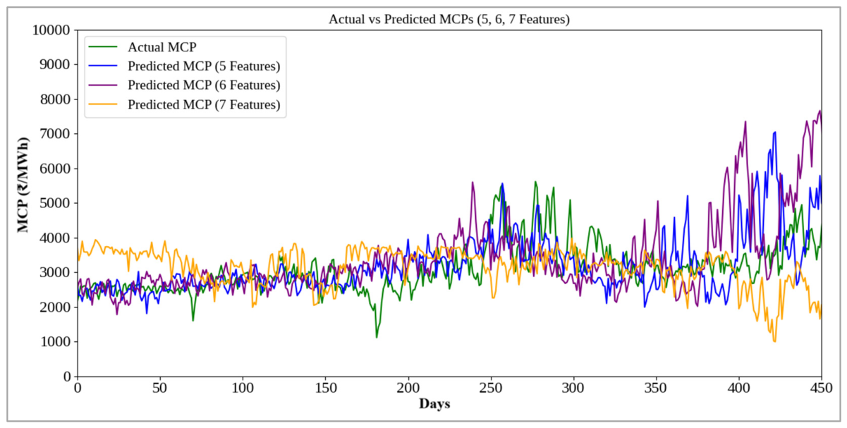
The trained model is tested to analyze accuracy utilizing energy price data for 450 days. It provides performance indices 474.36 (₹/MWh), 893.62 (₹/MWh), 15.14%, and 0.549 against MAE, RMSE, MAPE, and R². Now the CatBoost algorithm is provided with trained input data that includes features such as date, day of the week, type of day, MCP of the previous day, previous week’s same-day MCP, and previous month’s same day MCP. The model is then tested to observe the performance. The performance indices are improved from the previous step and are found to be ₹459.05/MWh, ₹856.90/MWh, 14.95%, and 0.587 against MAE, RMSE, MAPE, and R². Finally, the model is trained and tested using the features like date, day of week, type of day, MCP of the previous day, previous week’s same-day MCP, MCP of the same day of the previous month, and MCP of same-data of previous year. The performance indices are obtained as 566.17 (₹/MWh), 948.71 (₹/MWh), 16.52%, and 0.463 against MAE, RMSE, MAPE, and R² respectively. The CatBoost model’s performance is unsatisfactory compared to SARIMAX. Figure 6 displays the estimated and actual MCP values from the ML model employing the CatBoost algorithm.

Figure 6 clearly illustrates the underperformance of the CatBoost algorithm model. The model demonstrates significant deviations from the actual MCP values, particularly on specific days. Although the model, utilizing seven input features, attempts to align with the actual MCP trend, it notably fails in prediction during the days 50 to 55, 90 to 120, 150 to 200, 220 to 270, 295 to 300, 310 to 320, and 360 to 450. Figure 2, Figure 3, Figure 4, Figure 5 and Figure 6 imply the better performance of the SARIMAX model compared to the CatBoost algorithm irrespective of the input vector size.

3.2.2. Random Forest Algorithm

RF is an ensemble learning technique designed to improve accuracy and mitigate overfitting by combining multiple decision trees. The pre-processed training dataset is prepared as per Section 2.2, with features such as the day of the week, type of day, and MCP.

The data is now fed to the ML model that employs the RF algorithm. The ML models are tuned based on the hyperparameters tabulated in

Table 8. Hyperparameters used in the RF algorithm.

Hyperparameter		Best Hyperparameter
Max_depth	1, 2, 3, 4, 5	Max_depth
N_estimator	100, 200, 500, 700, 1000	N_estimator

. The model is configured with 1000 estimators, which aids in tuning it for better performance. The hyperparameters specified in Table 8, which include random_state, oob_score, max_depth, and n_estimator, are set to 0, True, 5, and 1000, respectively, to accelerate the speed and predictive power. The tuned model is now tested for its predictive performance, employing a 30% subset of the collected data with input features date, day of the week, type of day, MCP of the previous day, MCP of previous week’s same day. It provides performance indices 554.38 (₹/MWh), 689.45 (₹/MWh), 14.03%, and 0.403 against MAE, RMSE, MAPE, and R². In the subsequent step, the RF algorithm-based ML model is trained with six feature sets. The model is then tested to obtain MAE, RMSE, MAPE, and R² values of 625.29 (₹/MWh), 612.43 (₹/MWh), 14.21%, and 0.483, respectively. The seven input features are finally deployed to train and test the model. The MAE, RMSE, MAPE, and R² are obtained as ₹766.54/MWh, ₹682.45/MWh, 16.47%, and 0.389. The observations show the unsatisfactory performance of the RF model when compared to the SARIMAX model. Increasing the number of input features from five to seven has not yielded satisfactory improvements in performance indices. The predicted and actual values of MCP for the period from 1st July 2020 to 31st December 2021, about 450 days, are shown in Figure 7.

From Figure 7, it is evident that the model using the RF algorithm significantly deviates from the actual MCP, particularly during periods of 160 to 180, 240 to 250, 285 to 290, 310 to 320, 360 to 370, and 400 to 450. From the prediction graphs shown in Figure 4 and Figure 7, SARIMAX provides better results compared to the RF model.

3.2.3. LSTM Model

LSTM is a recurrent neural network that employs complex gating mechanisms to avoid vanishing gradient problems. The model is provided with training data that is pre-processed as per the procedure explained in Section 2.2. The LSTM architecture training parameters have been optimized using random search over predefined hyperparameters such as LSTM layers, neurons per LSTM, activation functions, window size, and epochs. The optimal configuration is selected based on the minimum validation error.

The final model consists of three stacked LSTM layers, each comprising 20 neurons, with ReLU activation functions applied to all hidden layers and a linear activation function to the output layer. The three-layer LSTM implementation details for predicting the market MCP are tabulated in

Table 9. LSTM model architecture.

Define the LSTM model	modelLstm = Sequential()
	modelLstm.add(LSTM(20,activation = ‘relu’, input_shape = (X_train.shape [1], 1)))
	modelLstm.add(Dense(1))
	modelLstm.compile(optimizer = ‘adam’,loss = ‘mape’)
Fit model	modelLstm.fit(X_train,y_train,epochs = 200, verbose = 0)
Demonstrate prediction	pred = modelLstm.predict(X_test).flatten()

. The optimizer and loss function are chosen as Adam and MAPE respectively. The model is trained for 200 epochs employing a window and input vector size of five each. The performance analysis is done for its prediction, deploying five, six, and seven features, respectively.

The MAE, RMSE, MAPE, and R² values for five input features are observed to be 367.21 (₹/MWh), 642.68 (₹/MWh), 14.06%, and 0.682. The model trained using six input vectors provides the performance indices as 413.15 (₹/MWh), 549.79 (₹/MWh), 11.93%, and 0.852 against MAE, RMSE, MAPE, and R². When the model is provided with seven input features, the indices are noted to be 351.94 (₹/MWh), 387.37 (₹/MWh), 9.62% and 0.88. The performance of the LSTM model is observed to improve consistently with the addition of input features. As the input feature count increases from five to seven, the model demonstrates a significant reduction in prediction errors. The LSTM model developed for MCP prediction with seven features produces MAE and RMSE higher than those seen with SARIMAX. The graph illustrating the actual values of MCP and predicted MCP with five, six, and seven input features from 1st July 2020 to 31st December 2021 for 450 days is depicted in Figure 8. The LSTM model provides a satisfactory forecast MCP when compared to SARIMAX, CatBoost, and RF models. The difference is clearly visible in Figure 4, Figure 6, Figure 7 and Figure 8.

3.2.4. BiLSTM Model

This section deals with the MCP prediction model using the BiLSTM. In connection with this, the model is provided with five, six, and seven input features corresponding to 5-year energy price data. The BiLSTM implementation details are tabulated in

Table 10. BILSTM model architecture.

Define the BiLSTM model	modelBiLstm = Sequential()
	modelBiLstm.add(Bidirectional(LSTM(13, activation = ‘relu’), input_shape = (X_train.shape [1], 1)))
	modelBiLstm.add(Dense(1))
	modelBiLstm.compile (Optimizer = ‘ADAM’, Loss = ‘MAPE’)
Fit model	modelBiLstm.fit(X_train,y_train, epochs = 100, verbose = 0)
Demonstrate prediction	pred= modelBiLstm.predict(X_test).flatten()

. The sliding window is a crucial component of BiLSTM networks that facilitates efficient modeling and extraction of features from sequential data. To achieve better prediction accuracy, a sliding window size of five is selected. The parameter settings after cross-validation of the input data set, with the optimum fold, are nine neurons and 100 epochs. The model is implemented by employing a ReLU activation function and the Adam optimizer.

The model is examined for its performance indices. The MAE, RMSE, MAPE, and R² values are found to be 367.2 (₹/MWh), 657.98 (₹/MWh), 13.36%, and 0.557, respectively, for an input vector size of five. Meanwhile, the values are obtained as ₹382.55/MWh, ₹519.19/MWh, 12.28%, and 0.798 respectively, when the model is provided with an input vector of size six. Concurrently, while deploying seven input features, the values are noted to be ₹443.75/MWh, ₹320.096/MWh, 11.81%, and 0.842.

The results demonstrate a notable improvement in predictive accuracy in the BiLSTM model as the number of input features increases from five to seven. The MAE increases significantly from ₹367.24/MWh to ₹443.75/MWh, while the RMSE reduces from 657.98 to 320.096. Similarly, the MAPE shows a decrease from 15.08% to 11.82%; moreover, the R² value improves from 0.557 with five input features to 0.842 with seven input features. It can be inferred that LSTM, when provided with seven features, provides improved performance compared to the BiLSTM model, which is also provided with seven features. The graph illustrates the actual values of MCP and predicted MCP, with five, six, and seven input features from 1 July 2020 to 31 December 2021 for 450 days, as depicted in Figure 9. Figure 9 indicates that the BiLSTM model delivers similar MCP predictions to the LSTM model. However, the graph shows deviations from actual MCP values for undershoots on days 55 to 70, 130 to 140, 160 to 180, and 205 to 240, as well as overshoots on days 80 to 90, 115 to 120, 155 to 165, 250 to 260, 265 to 280, 310 to 330, 355 to 400, and 415 to 430. It indicates that the BiLSTM model demonstrates slightly higher errors with varying input features in comparison to the LSTM model.

3.2.5. CNN–BiLSTM Model

The CNN–BiLSTM is a hybrid model that leverages the spatial feature extraction capabilities of CNNs and the temporal dependency modeling of BiLSTM to achieve improved prediction performance. The CNN–BiLSTM model configuration details are given in

Table 11. CNN–BILSTM model architecture.

Define the CNN model	model = Sequential () Model.Add (Conv1D(8, Kernal_Size = 3, Activation = ‘RELU’, Input_Shape = (X_Train.Shape [1], 1)))
Define BiLSTM model	model.add (Bidirectional(LSTM(13,activation = ‘relu’), input_shape = (X_train.shape [1], 1))) model.add (Dense(1)) model.compile(optimizer = ‘adam’, loss = ‘mape’)
Fit model	model.fit(X_train,y_train, epochs = 100, verbose = 0)
Demonstrate prediction	pred = model.predict(X_test).flatten)

. To attain prediction accuracy and improve computational efficiency, the sliding window and kernel sizes are considered five and three, respectively.

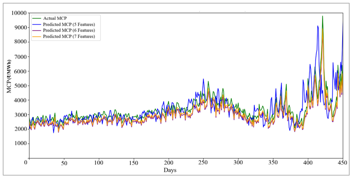
As listed in Table 11, the CNN –BiLSTM model employs eight and 13 neurons. With the activation function as ReLU and the optimizer as Adam, the model is trained for an epoch of 200. The CNN–BiLSTM model is tested with unseen data spanning from 1st July 2020 to 31st December 2021. The predictive performance of the CNN–BiLSTM model is systematically evaluated using five, six, and seven test input features. Feeding the dataset with five test input features, the model results an MAE of ₹370.13/MWh, an RMSE of ₹367.24/MWh, a MAPE of 11.16%, and R² of 0.763. Upon increasing the input feature set to six, the model provides indices of ₹413.15/MWh, ₹402.81/MWh, 11.28%, and 0.772, respectively. When the model is fed with seven features, the indices are found to be ₹375.43/MWh, ₹397.07/MWh, 11.03%, and 0.82. The observation illustrates that when the features are increased from five to seven, the performance indices of CNN-BiLSTM are found to improve. However, these values are not comparable to those observed from the LSTM model with a seven-input feature set. Figure 10 illustrates the actual values of MCP and predicted MCP, with five, six, and seven input features for 450 days.

Figure 10 indicates that the CNN-BiLSTM model provides satisfactory anticipated MCP values compared to RF and CatBoost models. The CNN-BiLSTM model with seven input features exhibits larger deviations between predicted and actual MCP values compared to the LSTM model with the same number of features. A more comprehensive assessment of the model’s performance is provided through observed MAE, RMSE, MAPE, and R² as shown in

Table 12. Performance indices of various models with five input feature sets.

Model	MAE (₹/MWh)	RMSE (₹/MWh)	MAPE (%)	R2
ARIMA	293.79	472.83	13.06	0.863
SARIMA	367.24	642.68	14.329	0.870
SARIMAX	545.57	824.17	12.39	0.745
CatBoost	474.36	893.62	15.14	0.549
RF	554.38	689.45	14.03	0.403
LSTM	367.21	642.6	14.06	0.682
BiLSTM	367.20	657.98	13.36	0.557
CNN-BiLSTM	370.13	367.24	11.16	0.763

,

Table 13. Performance indices of various models with six input feature sets.

Model	MAE (₹/MWh)	RMSE (₹/MWh)	MAPE (%)	R2
ARIMA	296.86	483.54	12.975	0.856
SARIMA	301.45	581.47	14.01	0.889
SARIMAX	508.05	438.47	11.51	0.79
CatBoost	459.05	856.9	14.95	0.587
RF	625.29	612.43	14.21	0.483
LSTM	413.15	549.79	11.93	0.852
BiLSTM	382.55	519.19	12.28	0.798
CNN-BiLSTM	411.05	402.81	11.28	0.772

and

Table 14. Performance indices of various models with seven input feature sets.

Model	MAE (₹/MWh)	RMSE (₹/MWh)	MAPE (%)	R2
ARIMA	299.45	497.31	13.467	0.869
SARIMA	293.79	580.53	13.82	0.883
SARIMAX	289.74	389.51	7.92	0.87
CatBoost	566.17	948.71	16.52	0.463
RF	766.54	682.45	16.47	0.389
LSTM	351.94	387.37	9.62	0.88
BiLSTM	443.75	320.09	11.81	0.842
CNN-BiLSTM	375.43	397.07	11.03	0.82

.

As displayed in Table 12, Table 13 and Table 14, the models trained on a set of five input features exhibit a limited capacity to capture complex temporal patterns, seasonal changes, and market-specific dynamics inherent in MCP data. Table 12, Table 13 and Table 14 show that the performance indices for models with five and six input features do not indicate a clear best-performing approach. A method that shows lower MAE or RMSE does not necessarily demonstrate the lowest MAPE or maximum R². This metric-dependent ranking is familiar in price forecasting and supports the need to interpret results using multiple indices under a consistent framework.

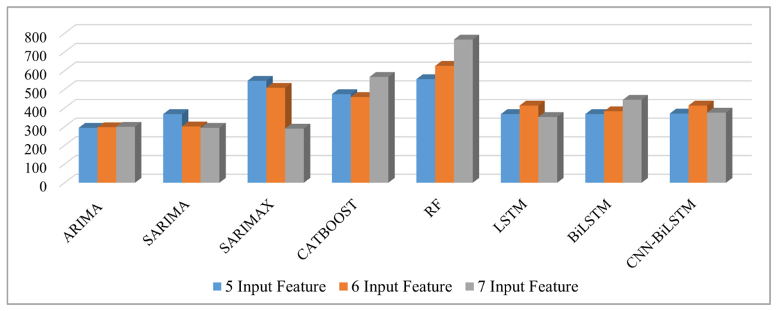
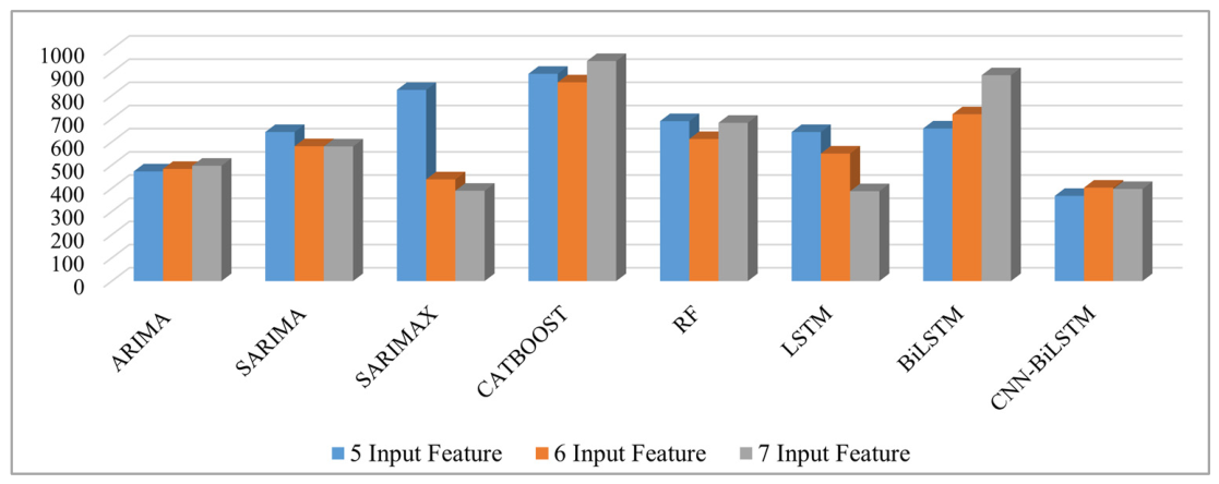
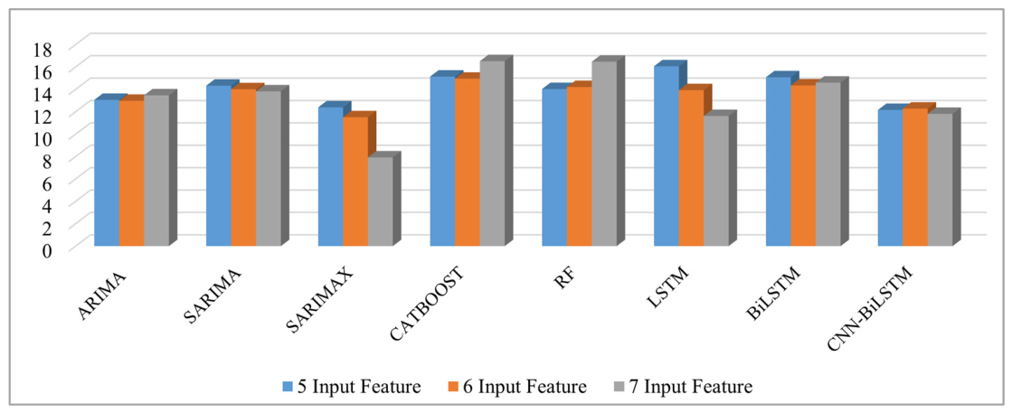
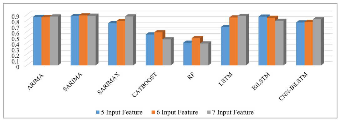
The LSTM model demonstrates improved accuracy in predicting MCP values when trained with seven input features. Moreover, it is found that increasing the input features further does not enhance the performance of the developed models. The feature importance analysis indicates that the lagged MCP variables dominate the predictive values, and the MCP of the previous day is the most influential input, showing that the model relies primarily on short-term price persistence to forecast MCP. All remaining predictors contribute marginally to the model accuracy. Adding calendar descriptors and multi-scale lagged MCP values helps the models to capture recurring weekly and seasonal structure and day-type effects, which improves the accuracy of energy price forecasts. The comparison of the indices for different models, tabulated in Table 12, Table 13 and Table 14, is represented in bar charts and is shown in Figure 11, Figure 12, Figure 13 and Figure 14.

Figure 11, Figure 12, Figure 13 and Figure 14 illustrates several key insights derived from the comparative analysis of forecasting models across varying input feature sets. Classical statistical approaches such as ARIMA, SARIMA, and SARIMAX demonstrate reasonable accuracy with limited input features, effectively modeling linear dependencies. However, deep learning models outperform them when richer contextual information is introduced. Among the models evaluated, the LSTM model demonstrates the lowest MAPE. This highlights its efficacy in minimizing the relative error, which is particularly beneficial in contexts where percentage-based accuracy is prioritized. In addition, the LSTM model consistently exhibits the most balanced and robust performance. It achieves the lowest MAE and RMSE, as well as the highest R², when trained on the comprehensive seven-feature set. This shows the superior capability to capture nonlinear temporal dependencies and generalize across diverse market conditions. The inclusion of additional features closes critical information gaps, enabling models to explain more variance, reduce residual errors, and improve proportional accuracy. Consequently, the LSTM model trained on a seven-feature set is identified as the most effective configuration for MCP forecasting with a MAE of ₹351.94/MWh, an RMSE of ₹387.37/MWh, a MAPE of 9.62%, and R² of 0.88. The continuous ranked probability score (CRPS) of 5.46% indicates that the model is well trained and reasonably accurate, with a relatively low deviation between the predicted probability distribution and the observed MCP.

Prediction interval normalized average width (PINAW) value of 0.1765 indicates that the predicted intervals are relatively narrow, reflecting a satisfactory level of sharpness in the probabilistic forecast. The probabilistic forecasting capability (PICP) of 85.07% indicates that approximately 85% of the actual MCP values fall within the predicted confidence intervals, demonstrating a satisfactory level of reliability. The experimental results indicate that increasing the feature set from five to seven results in a marginal improvement in performance indices. The behavior can be explained by the relative importance and information content of additional features, MCP of the same day in the previous month, and MCP of the same day in the same month of the previous year. These added features exhibit relatively low feature importance compared to the MCP of the previous day, indicating that their contribution to explaining price variability is limited. However, the slight improvements observed with seven features suggest that these additional variables still provide auxiliary contextual information, capturing weekly, seasonal, or long-term patterns that are not fully represented by short-term features. As a result, the model benefits from a small reduction in prediction error, even though the added features are not highly influential. From the methodological perspective, this reflects the tradeoff between feature richness and redundancy.

4. Conclusions

This work emphasizes the critical role of input feature selection in improving the efficacy of machine learning and deep learning models for projecting the market-clearing price in the Indian electricity market. A comprehensive assessment has been performed employing various statistical, machine learning, and deep learning methods for day-ahead MCP forecasting in the Indian electricity market. The models include autoregressive integrated moving average, seasonal autoregressive integrated moving average, seasonal autoregressive integrated moving average with exogenous variables, categorical boosting, random forest, long short-term memory, bidirectional long short-term memory, and hybrid convolutional neural network–bidirectional long short-term memory architecture. The market-clearing price dataset from 1 January 2017, to 31 December 2021, obtained from the Indian Energy Exchange, is deployed to create input vectors of sizes five, six, and seven. The features include date, day of the week, type of day, previous-day market-clearing price, same-weekday market-clearing price from the previous week, same-day market-clearing price from the previous month, and same-day market-clearing price from the previous year. The results show that changing the input feature set from five to seven significantly varies the performance matrices of the models. The long short-term memory network, modeled with seven features, performs the best of all models. The model delivers the lowest mean absolute error (₹351.94/MWh), root mean square error (₹387.37/MWh), along with the highest R² value (0.88), indicating its superior predictive accuracy and generalization capability. The lower prediction interval normalized average width value observed in the LSTM model suggests that the model provides more precise prediction intervals without excessively widening the bounds. A probabilistic forecasting capability value of 85.07% suggests that the model is able to capture the uncertainty associated with price variations to a reasonable extent. The above findings highlight the effectiveness of deep learning models, specifically the long short-term memory model, in capturing the nonlinear and temporal intricacies of Indian electricity market data. The study illustrates that deploying an optimal seven-feature input vector systematically enhances the forecasting accuracy across models and that further extension of feature set delivers only marginal benefits. Additionally, the observations reveal that appropriate feature engineering has a greater impact on MCP prediction accuracy than expanding the model complexity alone. Furthermore, the model can be extended to support multi-step forecasting and probabilistic prediction intervals, aiming to facilitate risk-aware decision-making in electricity markets.

References

1. Lai, L.L. Power System Restructuring and Deregulation: Trading, Performance and Information Technology; John Wiley & Sons: Hoboken, NJ, USA, 2001. [Google Scholar] [CrossRef] [Scilit]
2. Necoechea-Porras, P.D.; López, A.; Salazar-Elena, J.C. Deregulation in the energy sector and its economic effects on the power sector: A literature review. Sustainability 2021, 13, 3429. [Google Scholar] [CrossRef] [Scilit]
3. Conejo, A.J.; Sioshansi, R. Rethinking restructured electricity market design: Lessons learned and future needs. Int. J. Electr. Power Energy Syst. 2017, 98, 520–530. [Google Scholar] [CrossRef] [Scilit]
4. Ehsani, A.; Ranjbar, A.M.; Jafari, A.; Fotuhi-Firuzabad, M. Reliability evaluation of deregulated electric power systems for planning applications. Reliab. Eng. Syst. Saf. 2008, 93, 1473–1484. [Google Scholar] [CrossRef] [Scilit]
5. Niemeyer, V. Understanding Electric Utilities and Deregulation, Second Edition [Book Review]. IEEE Power Energy Mag. 2007, 5, 64–67. [Google Scholar] [CrossRef] [Scilit]
6. Karthikeyan, S.P.; Raglend, I.J.; Kothari, D.P. A review on market power in deregulated electricity market. Int. J. Electr. Power Energy Syst. 2013, 48, 139–147. [Google Scholar] [CrossRef] [Scilit]
7. Wehinger, L.A.; Hug-Glanzmann, G.; Galus, M.D.; Andersson, G. Modeling electricity wholesale markets with model predictive and profit maximizing agents. IEEE Trans. Power Syst. 2013, 28, 868–876. [Google Scholar] [CrossRef] [Scilit]
8. Reinisch, W.; Tezuka, T. Market power and trading strategies on the electricity market: A market design view. IEEE Trans. Power Syst. 2006, 21, 1180–1190. [Google Scholar] [CrossRef]
9. Aganagic, M.; Abdul-Rahman, K.H.; Waight, J.G. Spot pricing of capacities for generation and transmission of reserve in an extended Poolco model. IEEE Trans. Power Syst. 1998, 13, 1128–1135. [Google Scholar] [CrossRef] [Scilit]
10. Lekshmi, R.R.; Balamurugan, S. Load following under different market models in a restructured power system. J. Electr. Syst. 2018, 14, 72–85. [Google Scholar]
11. Yang, Y.; Bao, M.; Song, Y.; Ding, Y.; Lin, Z.; Shao, C. Review of information disclosure in different electricity markets. Energies 2018, 11, 3424. [Google Scholar] [CrossRef] [Scilit]
12. Weron, R. Electricity price forecasting: A review of the state-of-the-art with a look into the future. Int. J. Forecast. 2014, 3, 1030–1081. [Google Scholar] [CrossRef] [Scilit]
13. Mi, H.; Chen, S.; Li, Q.; Hou, S.; Zheng, L.; Xu, C.; Yan, Z.; Li, C. Strategic bidding by predicting locational marginal price with aggregated supply curve. Energy 2024, 304, 162–181. [Google Scholar] [CrossRef] [Scilit]
14. Kotur, D.; Zarkovic, M. Neural network models for electricity prices and loads short and long-term prediction. In Proceedings of the 4th International Symposium Environment Friendly Energies and Applications, Belgrade, Serbia, 14–16 September 2016; pp. 1–5. [Google Scholar] [CrossRef] [Scilit]
15. Walter, V.; Wagner, A. Probabilistic simulation of electricity price scenarios using Conditional Generative Adversarial Networks. Energy AI 2024, 18, 100422. [Google Scholar] [CrossRef] [Scilit]
16. Kuo, P.-H.; Huang, C.-J. An electricity price forecasting model by hybrid structured deep neural networks. Sustainability 2018, 10, 1280–1297. [Google Scholar] [CrossRef] [Scilit]
17. Wang, Z.; Matsuhashi, R. Low-energy miniature wearable air-conditioner with direct cold-air delivery: A novel water–electricity hybrid energy system. Build. Environ. 2026, 297, 114590. [Google Scholar] [CrossRef] [Scilit]
18. Jan, F.; Shah, I.; Ali, S. Short-term electricity prices forecasting using functional time series analysis. Energies 2022, 3, 3423. [Google Scholar] [CrossRef] [Scilit]
19. Leal, P.; Castro, R.; Lopes, F. Influence of increasing renewable power penetration on the long-term Iberian electricity market prices. Energies 2023, 16, 1054. [Google Scholar] [CrossRef] [Scilit]
20. Contreras, J.; Espinola, R.; Nogales, F.J.; Conejo, A.J. ARIMA models to predict next-day electricity prices. IEEE Trans. Power Syst. 2003, 18, 1014–1020. [Google Scholar] [CrossRef] [Scilit]
21. Lekshmi, R.R.; Bansi, C. Demand management planning system for a meat factory based on the predicted market price under Indian market scenario. In Lecture Notes in Electrical Engineering, Proceedings of the 4th International Conference Communication, Computing and Electronics Systems, Coimbatore, India, 15 March 2023; Springer: Singapore, 2023; pp. 439–450. [Google Scholar] [CrossRef] [Scilit]
22. Das, R.; Bo, R.; Chen, H.; Rehman, W.U.; Wunsch, D. Forecasting nodal price difference between day-ahead and real-time electricity markets using long-short term memory and sequence-to-sequence networks. IEEE Access 2022, 10, 832–843. [Google Scholar] [CrossRef] [Scilit]
23. Hu, B.; Gong, Y.; Chung, C.Y.; Noble, B.F.; Poelzer, G. Price-maker bidding and offering strategies for networked microgrids in day-ahead electricity markets. IEEE Trans. Smart Grid 2021, 12, 5201–5211. [Google Scholar] [CrossRef] [Scilit]
24. Zhang, C.; Li, R.; Shi, H.; Li, F. Deep learning for day-ahead electricity price forecasting. IET Smart Grid 2020, 3, 462–469. [Google Scholar] [CrossRef] [Scilit]
25. Yadav, D.; Mekhilef, S.; Singh, B.; Rawa, M. Deep reinforcement learning and energy price prediction. In Artificial Intelligence-Based Smart Power Systems; Wiley-IEEE Press: Hoboken, NJ, USA, 2023; pp. 207–231. [Google Scholar] [CrossRef] [Scilit]
26. Al-Shakhs, M.; El-Hawary, M.E. Innovations-based neural network seasonal day-ahead marginal price forecasting. Electr. Power Compon. Syst. 2015, 43, 588–593. [Google Scholar] [CrossRef] [Scilit]
27. Abdoli, G.; MehrAra, M.; Ardalani, M.E. Comparing the prediction accuracy of LSTM and ARIMA models for time-series with permanent fluctuation. Gênero Direito 2020, 9. [Google Scholar] [CrossRef] [Scilit]
28. Kottath, R.; Singh, P. A meta-heuristic learning approach for short-term price forecasting. In Soft Computing: Theories and Applications; Springer: Singapore, 2022; pp. 131–333. [Google Scholar] [CrossRef] [Scilit]
29. Smitha, E.P.; Raglend, I.J. Sequential wavelet-ANN with embedded ANN-PSO hybrid electricity price forecasting model for Indian energy exchange. Neural Comput. Appl. 2017, 4, 28–77. [Google Scholar] [CrossRef] [Scilit]
30. Arvanitidis, A.I.; Bargiotas, D.; Tomtsis, D.; Kontogiannis, S.; Fevgas, A.; Alamaniotis, M. Optimized data-driven models for short-term electricity price forecasting based on signal decomposition and clustering techniques. Energies 2022, 15, 7929. [Google Scholar] [CrossRef] [Scilit]
31. Zhang, C.; Fu, Y. Probabilistic electricity price forecast with optimal prediction interval. IEEE Trans. Power Syst. 2023, 39, 442–452. [Google Scholar] [CrossRef] [Scilit]
32. Wang, B.; Wang, J. Energy futures and spots prices forecasting by hybrid SW-GRU with EMD and error evaluation. Energy Econ. 2020, 90, 104827. [Google Scholar] [CrossRef] [Scilit]
33. Kuno, S.; Tanaka, K.; Yamada, Y. Effectiveness and feasibility of market makers for P2P electricity trading. Energies 2022, 15, 4218. [Google Scholar] [CrossRef] [Scilit]
34. Gupta, G.; Singh, A. Modernizing India’s electricity market: Opportunities for market-based PPAs, contracts for difference, and revenue-sharing contracts. Electr. J. 2025, 38, 107505. [Google Scholar] [CrossRef] [Scilit]
35. Biswas, P.; Sharma, C.; Padhan, H. Electricity shortages, price asymmetries, and behavioral responses in the Indian energy market. Financ. Res. Lett. 2026, 90, 109396. [Google Scholar] [CrossRef] [Scilit]
36. Lekshmi, R.R.; Swathy, S.; Lakshmi, B.; Sai, N.V.; Vijaykumar, V.S. Market clearing mechanism considering congestion under deregulated power system. Procedia Comput. Sci. 2018, 143, 686–693. [Google Scholar] [CrossRef] [Scilit]
37. Lekshmi, R.R.; Balamurugan, S.; Sasi, K.K. Decentralised automatic generation control strategy for a three area bilateral power market. In Proceedings of the Biennial International Conference on Power and Energy Systems: Towards Sustainable Energy, Bengaluru, India, 21–23 January 2016; pp. 1–6. Available online: http://ieeexplore.ieee.org/abstract/document/7516502/ (accessed on 27 July 2026).
38. Lekshmi, R.R.; Balamurugan, S. Single stage auction clearing model for electricity market considering congestion. Results Eng. 2025, 25, 104279. [Google Scholar] [CrossRef] [Scilit]
39. Subeekrishna, M.P.; Lekshmi, R.R. Data-Driven Approach to Predict Spot Market Price in Indian Electricity. In Proceedings of the IEEE International Conference on Electrical, Electronics, Communication and Computers, Roorkee, India, 26–27 August 2023; pp. 1–5. [Google Scholar] [CrossRef] [Scilit]
40. Anamika; Kumar, N. Market-clearing price forecasting for Indian electricity markets. Adv. Intell. Syst. Comput. 2017, 479, 633–642. [Google Scholar] [CrossRef] [Scilit]
41. Wang, L.; Zou, H.; Su, J.; Li, L.; Chaudhry, S.S. An ARIMA-ANN hybrid model for time series forecasting. Syst. Res. Behav. Sci. 2013, 30, 244–259. [Google Scholar] [CrossRef] [Scilit]
42. Jakasa, T.; Androcec, I.; Sprcic, P. Electricity price forecasting ARIMA model approach. In Proceedings of the 8th International Conference on the European Energy Market (EEM-IEEE), Zagreb, Croatia, 25–27 May 2011; pp. 222–225. [Google Scholar] [CrossRef] [Scilit]
43. Yin, C.; Liu, K.; Zhang, Q.; Hu, K.; Yang, Z.; Yang, L.; Zhao, N. SARIMA-based medium- and long-term load forecasting. Strateg. Plan. Energy Environ. 2023, 42, 283–306. [Google Scholar] [CrossRef] [Scilit]
44. McHugh, C.; Coleman, S.; Kerr, D.; McGlynn, D. Forecasting day-ahead electricity prices with a SARIMAX model. In Proceedings of the IEEE Symposium Series on Computational Intelligence (SSCI), Xiamen, China, 6–9 December 2019; pp. 1523–1529. [Google Scholar] [CrossRef] [Scilit]
45. Castelli, M.; Groznik, A.; Popovič, A. Forecasting electricity prices: A machine learning approach. Algorithms 2020, 13, 119–135. [Google Scholar] [CrossRef] [Scilit]
46. Zhang, F.; Fleyeh, H.; Bales, C. A hybrid model based on bidirectional long short-term memory neural network and CatBoost for short-term electricity spot price forecasting. J. Oper. Res. Soc. 2020, 73, 301–325. [Google Scholar] [CrossRef] [Scilit]
47. Chang, Z.; Zhang, Y.; Chen, W. Electricity price prediction based on hybrid model of Adam optimized LSTM neural network and wavelet transform. Energy 2019, 2, 187–195. [Google Scholar] [CrossRef] [Scilit]
48. Wang, Z.; Yamane, M.; Ajisaka, T.; Nakata, M.; Matsuhashi, T.; Mae, R. Enhanced day-ahead electricity price forecasting using a convolutional neural network–long short-term memory ensemble learning approach with multimodal data integration. Energies 2024, 17, 2687. [Google Scholar] [CrossRef] [Scilit]
49. Ubrani, A.; Motwani, S. LSTM- and GRU-based time series models for market clearing price forecasting of Indian deregulated electricity markets. Adv. Intell. Syst. Comput. 2019, 898, 693–700. [Google Scholar] [CrossRef] [Scilit]
50. Rekha, R.P.; Bhumika, C.P. Data-driven forecasting for grid stability: Implementing XGBoost in smart energy systems. In Proceedings of the International Conference on Modern Sustainable Systems (CMSS), Shah Alam, Malaysia, 12–14 October 2025; pp. 139–146. [Google Scholar] [CrossRef] [Scilit]
51. Gurung, B.; Mishra, P.; Shanmugam, P.K. Predictive analysis of market clearing price in the Indian electricity market using time series algorithms. In Proceedings of the International Conference on Sustainable Energy: Energy Transition and Net-Zero Climate Future (ICUE), Pattaya City, Thailand, 21–23 October 2024; pp. 1–5. [Google Scholar] [CrossRef] [Scilit]
52. Tiwari, A.K.; Eapen, L.M.; Nair, S.R. Electricity consumption and economic growth at the state and sectoral level in India: Evidence using heterogeneous panel data methods. Energy Econ. 2021, 94, 105064. [Google Scholar] [CrossRef] [Scilit]
53. Belyaev, L.S. Electricity markets [The business scene]. IEEE Power Energy Mag. 2007, 5, 16–26. [Google Scholar] [CrossRef] [Scilit]
54. Jain, R.; Nandan, A. Electricity prices and firms’ decisions and outcomes: The case of India after a decade of the Electricity Act. Energy Econ. 2020, 91, 104915. [Google Scholar] [CrossRef] [Scilit]
55. Rajan, P.; Chandrakala, K.R.M.V. Statistical model approach of electricity price forecasting for Indian electricity market. In Proceedings of the IEEE Madras Section Conference (MASCON), Chennai, India, 4–6 August 2021; pp. 1–5. [Google Scholar] [CrossRef] [Scilit]
56. Wang, P.; Xu, K.; Ding, Z.; Du, Y.; Liu, W.; Sun, B.; Zhu, Z.; Tang, H. An online electricity market price forecasting method via random forest. IEEE Trans. Ind. Appl. 2022, 58, 7013–7021. [Google Scholar] [CrossRef] [Scilit]
57. Chen, Y.; Zhao, H.; Zhou, R.; Xu, P.; Zhang, K.; Dai, Y.; Zhang, H.; Zhang, J. CNN-BiLSTM short-term wind power forecasting method based on feature selection. IEEE J. Radio Freq. Identif. 2022, 6, 922–927. [Google Scholar] [CrossRef] [Scilit]
58. Devanathan, B.; Suyampulingam, A.; Selvaraj, P.; Karuppasamy, I.; Ilamparithi, T. A Cloud-Integrated Virtual Framework for LSTM-Driven Solar Forecasting and Residential Energy Management. IEEE Access 2025, 13, 151055–151071. [Google Scholar] [CrossRef] [Scilit]
59. Borkini, D.; Nemethi, M.; Michalconok, G.; Mezentseva, O. Adding additional features to improve time series prediction. Res. Pap. Fac. Mater. Sci. Technol. Trnava Slovak Univ. Technol. Bratisl. 2019, 27, 72–78. [Google Scholar] [CrossRef] [Scilit]
Figure 1. Input sample dataset.
Energies 19 03910 g001
Figure 2. Actual and predicted MCP values for the ARIMA model.
Energies 19 03910 g002
Figure 3. Actual and predicted MCP values for the SARIMA model.
Energies 19 03910 g003
Figure 4. Actual and predicted MCP values for the SARIMAX model.
Energies 19 03910 g004
Figure 5. Input dataset considering the type of day.
Energies 19 03910 g005
Figure 6. Actual and predicted MCP values for the CatBoost model.
Energies 19 03910 g006
Figure 7. Actual and predicted MCP values for the RF model.
Energies 19 03910 g007
Figure 8. Actual and predicted MCP values for the LSTM model.
Energies 19 03910 g008
Figure 9. Actual and predicted MCP values for the BiLSTM model.
Energies 19 03910 g009
Figure 10. Actual and predicted MCP values for CNN-BiLSTM model.
Energies 19 03910 g010
Figure 11. Comparison of observed MAE from models trained with 5, 6, and 7 input features.
Energies 19 03910 g011
Figure 12. Comparison of observed RMSE from models trained with five, six, and seven input features.
Energies 19 03910 g012
Figure 13. Comparison of observed MAPE from models trained with five, six, and seven input features.
Energies 19 03910 g013
Figure 14. Comparison of observed R2 from models trained with five, six, and sseven input features.
Energies 19 03910 g014