Smart Distribution Panel Design for Integrating Non-OCPP EV Chargers into Real-Time Energy Management Systems: Hardware Implementation and Voltage Impact Analysis ^†

Abstract

Non-OCPP electric vehicle (EV) chargers lack site-integrated monitoring and supply-control, limiting their use in real-time energy management systems. This paper presents a Smart Distribution Panel that closes this gap via panel-side observability and an operator-commanded single-phase/three-phase (1$\mathsf{\Phi }$/3$\mathsf{\Phi }$) supply reconfiguration. In a single-site feasibility study, the panel is characterised with one consumer Tesla Wall Connector Gen 3 (Non-OCPP) and one Tesla Model Y at a Taiwan 3$\mathsf{\Phi }$3W 220 V site, using a CPM-80 meter (IEC 62053-22 class 0.2S), interlocked contactors, an e-stop relay, and a Raspberry Pi 4 data path. Phase-mode transitions interrupt charging for ∼5 s, resolved by the IEC 61851-1 handshake. A 74.5-min stepwise session—driven by the OCPP DC fast charger with the Non-OCPP Wall Connector idle—yields a site-specific ensemble PCC-bus sensitivity $V=224.85-0.147P$ ($R^2=0.991$), characterising the site + DC-charger + base-load ensemble observed through the panel’s metering rather than the panel’s Non-OCPP path; an OpenDSS bounded sanity check gives an upper-bound slope of 0.26–0.28 V/kW. The one-second data stream supports a non-autoregressive (Non-AR) LSTM residual-detection layer (8-seed RMSE $0.310\pm 0.084$ V). A synthetic voltage-drop sensitivity sweep (ROC-AUC 0.81–0.97) characterises sensitivity to injected perturbations, not real-world fault detection. Feasibility is demonstrated only for the tested single-site configuration; multi-site, multi-EVSE, multi-EV generalisation, autonomous demand response, and OCPP session-level features are not demonstrated and are stated as future work.

1. Introduction

The global transition toward carbon neutrality has accelerated the adoption of electric vehicles (EVs) at an unprecedented rate. Governments worldwide have committed to ambitious targets for EV deployment, with several nations planning to phase out internal combustion engine vehicles by 2035 [1,2]. This rapid electrification of transportation, however, introduces significant challenges for electrical-distribution networks, particularly at the building and campus level where charging infrastructure is most commonly deployed [3,4].

EV charging stations impose substantial instantaneous loads on distribution systems. A single DC fast charger can draw 30–150 kW, and newer ultra-fast charging standards (Tesla V4 Superchargers, CCS-based extreme fast charging, the CharIN Megawatt Charging System for heavy-duty vehicles) extend per-port DC power to 350–400 kW and beyond, while even Level 2 AC chargers operating at 7–11 kW—and increasingly at up to 19.2 kW in modern North American Level 2 deployments such as the Tesla Wall Connector and the Wallbox Pulsar Plus configured for an 80 A 240 V split-phase service—can create notable voltage perturbations when multiple units operate simultaneously on the same feeder [5,6]. The permissible voltage band of ±5% specified by power-quality standards defines the operating envelope that distribution-side instrumentation is designed to protect [7,8]. At the campus deployment studied here, the empirical voltage drop remained a small fraction of this band (1.5% at 28 kW of aggregate site charging load, driven by the OCPP DC fast charger with the Non-OCPP Wall Connector idle); however, the slope of the voltage–load relationship implies that coincident peak loads aggregating multiple chargers on the same feeder, or pairing with other non-EV loads, can readily approach the ±5% limit. Such a slope is a property of the site and its prevailing load mix rather than of any single charger or of the panel instrumentation itself; panel-side observability is valuable because it exposes this site-level trend to the EMS in real time, so that operator-commanded curtailment can act before the envelope is exhausted. Consequently, effective energy management systems (EMSs) that provide real-time monitoring and operator-commanded control of EV charging infrastructure have become essential [9,10].

Modern EMS frameworks for EV charging typically rely on the Open Charge Point Protocol (OCPP) to communicate with charging stations [11]. The OCPP is an open communication standard that enables centralised management of charging stations, providing capabilities such as remote start/stop, power metering, load balancing, and firmware updates [12]. OCPP-compliant chargers report their operational status—including voltage, current, power, and charging session data—through standardised messages, enabling seamless integration into EMS platforms [13].

However, a significant portion of the deployed EV charger installed base consists of devices that do not expose an OCPP endpoint to a third-party EMS, regardless of whether the manufacturer has obtained an OCPP certification. The majority of residential and small commercial Level 2 AC chargers historically shipped as consumer-grade products without standardised communication protocols [14,15]. The Tesla Wall Connector Gen 3, one of the most widely deployed residential and commercial EV chargers globally, is a representative example. We note that Tesla has obtained Open Charge Alliance certifications for some product variants—specifically, the Universal Wall Connector (OCPP 1.6J certificate OCA.0016.0900.CS, registered 30 September 2024) and the V4 Supercharger (OCPP 2.0.1 certificate OCA.0201.0103.CS, registered 1 July 2025) [16]—but the public integration path documented by Tesla is the proprietary Fleet API rather than a third-party Charging Station Management System (CSMS)-accessible OCPP endpoint [17,18]. The consumer Wall Connector Gen 3, which is the unit deployed in the present study, has no published OCPP support and is effectively Non-OCPP for facility-level EMS integration [19]. The Smart Panel approach addressed in this paper therefore remains directly relevant for: (i) the substantial Wall Connector Gen 3 installed base; (ii) other Non-OCPP chargers (ChargePoint Home Flex, Grizzl-E, legacy JuiceBox and Wallbox Pulsar units); and (iii) facilities requiring vendor-independent power-quality monitoring beyond what manufacturer firmware exposes. Such a hardware-level integration approach is, in principle, applicable across different electric vehicle supply equipment (EVSE) brands because it instruments the upstream electrical supply rather than the charger itself; however, the present work is experimentally characterised only with the Tesla Wall Connector Gen 3 and one Tesla Model Y, and we do not claim multi-brand demonstration (see Section 4.1). For facility managers seeking unified monitoring across heterogeneous charger fleets, the panel-side approach remains a useful complement to OCPP-side current-limiting [20,21].

One might argue that the straightforward solution is to replace Non-OCPP chargers with OCPP-compliant alternatives. However, this approach is impractical even at the residential tier, for three reasons. (1) Cost. Residential OCPP-capable Level 2 chargers (e.g., Wallbox Pulsar Plus or ChargePoint Home Flex with installer-activated OCPP) typically retail at USD 549–749, and commercial-grade OCPP chargers (such as ChargePoint CT4000 dual-port pedestals used in facility deployments) range from USD 2000 to USD 5000 excluding installation labour; fleet-wide replacement is expensive at either grade. (2) Owner preference. Many Non-OCPP chargers, such as the Tesla Wall Connector (USD 420–500 retail), are preferred by EV owners for their superior charging performance, brand compatibility, and lower acquisition cost. (3) Growing installed base. The Non-OCPP installed base continues to grow as consumers purchase chargers independently of facility management decisions. A practical EMS must therefore accommodate the heterogeneous charger ecosystem as it exists, rather than requiring homogeneous OCPP compliance.

This limitation creates a critical gap in modern EMS deployments. As EV adoption grows, many facilities will inevitably deploy a mix of OCPP-compliant and Non-OCPP chargers. Without a mechanism to integrate Non-OCPP chargers, the EMS can only manage a subset of the charging load, undermining the effectiveness of demand response programs, voltage regulation strategies, and load balancing algorithms [22,23].

The existing literature on EV charging infrastructure and EMS design has focused predominantly on OCPP-compliant systems. In the domain of EMS optimisation and smart charging, several studies have proposed advanced frameworks incorporating deep reinforcement learning [9,20], multi-agent systems [15,24], and IoT-based architectures [25] for optimising EV charging operations. Smart charging strategies for power management in distribution grids with high renewable penetration have also been investigated [26]. Virtual power plant concepts and demand response mechanisms have been explored for coordinating distributed energy resources including EV chargers [27,28,29,30]. Demand management for buildings with EV charging and renewable sources has been studied, yet these works uniformly assume protocol-compliant chargers [31,32].

In the domain of voltage impact and distribution network studies, research on voltage stability with EV charging loads has quantified the impact of fast charging on power quality [19,33,34,35], and optimal placement strategies for charging stations have been proposed to minimise grid impact [36,37]. Voltage impact assessment of high-power EV charging on distribution grids has been conducted [38]. Community-level and microgrid energy management with renewable integration has been explored [39,40,41,42,43,44,45,46], including EV charging infrastructure planning [47] and grid fault ride-through with energy storage [48].

In the domain of EV charging hardware, significant research has addressed converter topologies for fast chargers [49], high-voltage station standards and rectifier designs [50], multifunctional on-board chargers with vehicle-to-vehicle capability [51], black-box small-signal modeling of battery charger dynamics [52], PV-grid battery charging system designs [53], and integrated EV charging stations with grid-interfacing inverters [54].

Preliminary aspects of this work were presented in our earlier conference publications [55,56]. The relationship to the journal version is summarised in

Table 1. Relationship between the prior conference publications and the present journal version.

Aspect	SDSE 2023 [55]	CPEEE 2024 [56]	This Work
Smart Panel hardware design (components, e-stop, on-delay, schematic)	Early “Intelligent Switchboard” prototype, high level	Not covered	Complete design + new vector schematic + IEC standards alignment
Phase-reconfiguration procedure (∼5 s EV-perspective interrupt, IEC 61851-1)	Not described	Not described	New
Voltage impact data	Anecdotal	Single-day, descriptive	74.5 min stepwise, in-session $V=224.85-0.147P$, $R^2=0.991$; cross-day check
OpenDSS bounded sanity check	Not performed	Not performed	New (0.26–0.28 V/kW upper bound)
Non-AR LSTM residual detector	Not present	Not present	New (8-seed mean ± std)
Baseline ladder (Persistence, $\Delta V=I·R$, Linear, Ridge, Lasso, LightGBM, RNN, GRU, LSTM)	Not present	Not present	New
Synthetic voltage-drop sensitivity sweep	Not present	Not present	New
Commercial-alternative comparison (smart meter + contactor; HMS Intesis)	Not present	Not present	New

: the conference papers introduced the early “Intelligent Switchboard” concept and a high-level voltage impact narrative, respectively, while the present journal version contributes the complete Smart Panel hardware design with new vector schematic and IEC standards alignment, the explicit phase-reconfiguration procedure (Section 2.2), the 74.5-min stepwise voltage impact characterisation, the OpenDSS bounded sanity check (Section 3.2), the Non-AR LSTM residual-detection layer with 8-seed mean ± std reporting and a Persistence/physics baseline ladder (Section 3.3), the synthetic voltage-drop sensitivity sweep, and the commercial-alternative comparison (Section 4.2). By component count, well over 80% of the journal manuscript content is new relative to the conference papers.

Despite this extensive body of work, a notable gap emerges: the overwhelming majority of EMS studies assume that the EV charger under management supports a standardised communication protocol (typically OCPP) or possesses native smart capabilities. Commercial smart-meter + contactor products and protocol-translation gateways such as the HMS Intesis OCPP-to-Modbus bridge address adjacent problems but do not provide supply-side $1\mathsf{\Phi }$/$3\mathsf{\Phi }$ reconfiguration of a single fixed-wired EVSE, which is the headline distinctive capability of the Smart Panel presented here (a detailed comparison is given in Section 4.2).

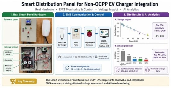
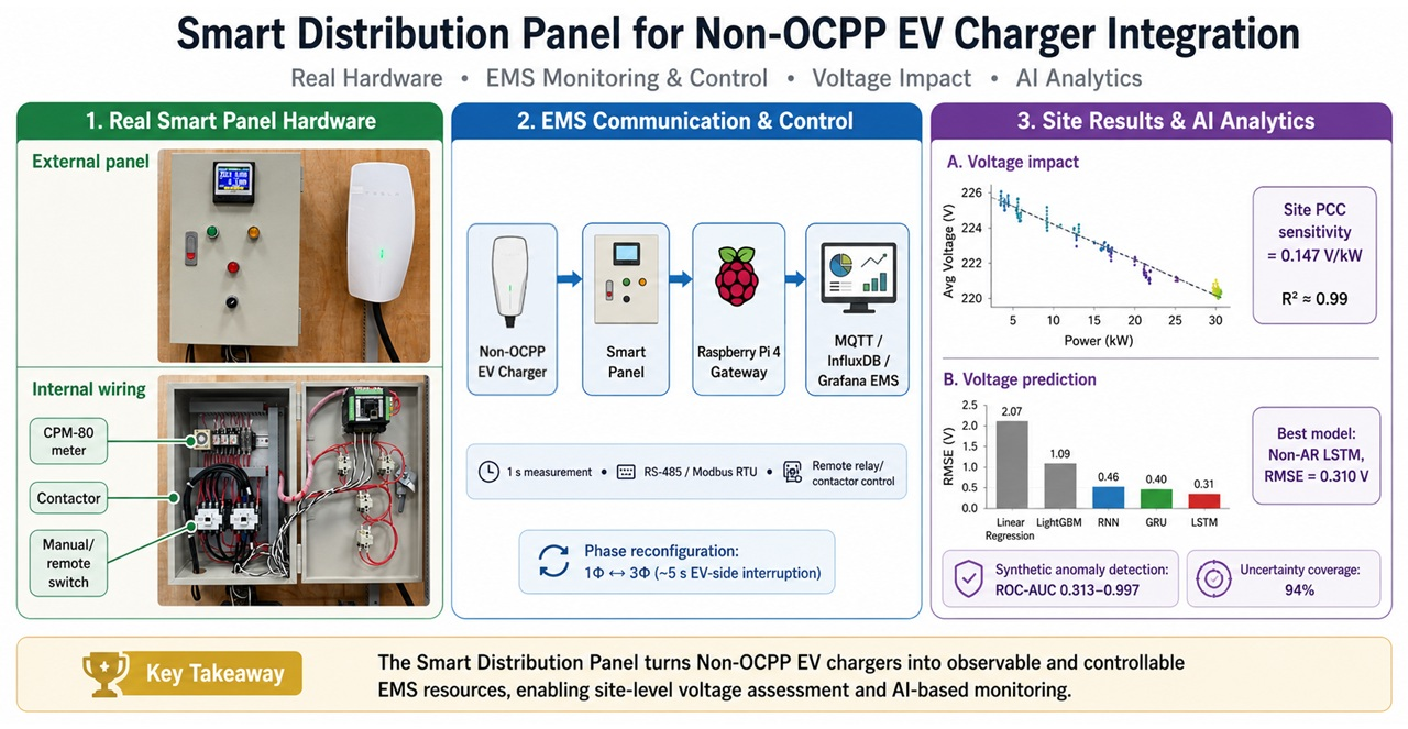
This paper presents the design, implementation, and experimental characterisation of a Smart Distribution Panel for panel-side observability and operator-commanded supply reconfiguration of Non-OCPP EV chargers. The headline hardware capability is an electromagnetic $1\mathsf{\Phi }$ (7 kW)/$3\mathsf{\Phi }$ (11 kW) reconfiguration of the EVSE supply via mechanically interlocked contactors with a configurable on-delay timer for mode-cycle protection, an emergency-stop relay, and a per-phase miniature circuit breaker (MCB) protection set. A phase-mode transition interrupts EV charging for approximately five seconds, resolved by the standard IEC 61851-1 charging-state handshake. The key contributions of this work are as follows:

• Smart Distribution Panel with $1\mathsf{\Phi }$/$3\mathsf{\Phi }$ supply reconfiguration. A hardware design with mechanically interlocked contactors, configurable on-delay mode-cycle protection, an e-stop relay, per-phase MCBs, and a CPM-80 (IEC 62053-22 class 0.2S) capturing 29 electrical parameters at 1 s; the panel provides observability and supply-side control, not OCPP session-layer features (authorisation, transaction reporting, charge-profile negotiation, firmware updates, session-level metering).
• Multi-protocol EMS architecture. A unified data path integrating the Non-OCPP charger via a Raspberry Pi 4 gateway (RS-485/Modbus RTU → MQTT → Telegraf → InfluxDB → Grafana) alongside the OCPP 1.6J path for compliant chargers, presenting a single operator view at a one-second resolution.
• Operator-commanded site-level demand management. Operator-issued $1\mathsf{\Phi }$ (7 kW)/$3\mathsf{\Phi }$ (11 kW) demotion compresses concurrent session draw so more vehicles can charge under a fixed contracted capacity, complementing OCPP-side current-limiting; autonomous closed-loop demand response is not demonstrated and is stated as future work.
• Voltage impact characterisation with bounded sanity check. A 74.5-min stepwise load reduction session—driven by the OCPP DC fast charger with the Non-OCPP Wall Connector idle, i.e., a characterisation of the overall site PCC obtained through the panel’s metering, not an evaluation of the panel’s reconfiguration path—yields $V=224.85-0.147P$ ($R^2=0.991$, $p=2.8\times {10}^{-6}$), a 3.33 V drop (1.49%) over a 24 kW range; an OpenDSS bounded sanity check using measured cable parameters and the 75 kVA Shihlin transformer ($Z\%=4.8\%$, Dyn1) gives a conservative upper bound of 0.26–0.28 V/kW. The empirical slope is interpreted as an ensemble effective sensitivity across heterogeneous paths; its position at approximately 55% of the upper bound is consistent with actual path impedance sitting below the upper-bound assumption (the contributing mechanisms are analysed in Section 3.2).

Additionally, the high-resolution Smart Panel data stream supports a non-autoregressive (Non-AR) Long Short-Term Memory (LSTM) residual-detection layer. 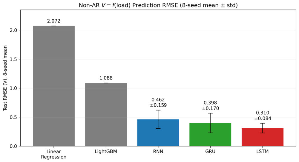The Non-AR LSTM learns the conditional expectation $\mathbb{E}$[V ∣ load history, time-of-day] from load-side features only—past voltage values are deliberately excluded from the input to prevent the model from trivially copying autocorrelation, so that prediction residuals reflect deviations from the learned $V=f(\mathrm{load},\mathrm{time})$ relationship and not simply from yesterday’s value. 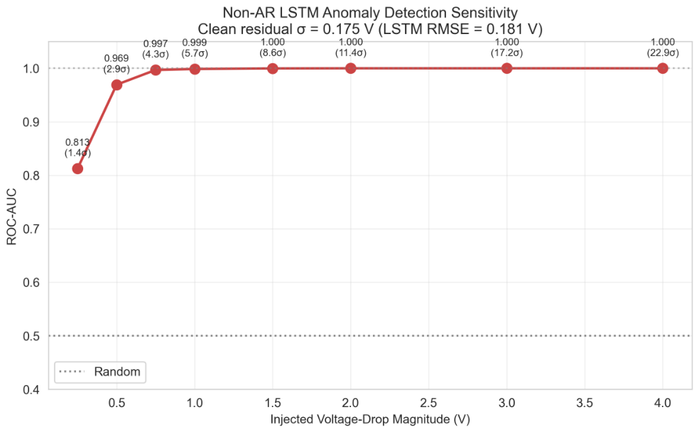Across eight random seeds the Non-AR LSTM achieves a test RMSE of $0.310\pm 0.084$ V; Naive Persistence achieves a lower raw RMSE (0.080 V) but uses no load features and is structurally unsuitable for the residual-detection task (Section 3.3). A synthetic voltage-drop sensitivity sweep characterises sensitivity to perturbations of 0.25–1.5 V (ROC-AUC 0.81–0.97); these values measure sensitivity to a synthetic perturbation class, not real-world fault detection. The LSTM analytics layer is reported as a downstream application of the Smart Panel’s data stream rather than as an independent contribution.

The remainder of this paper is organised as follows. Section 2 presents the system architecture, Smart Panel design, and experimental methodology. Section 3 presents the experimental results and analysis. Section 4 discusses the findings and their implications. Section 5 concludes this paper.

2. Materials and Methods

This section presents the complete system architecture of the proposed EMS, with particular emphasis on the Smart Distribution Panel that constitutes the core hardware contribution of this work. The system integrates both OCPP and Non-OCPP EV charging stations under a unified monitoring and control framework. The experimental setup and methodology are also described.

2.1. Energy Management System Architecture

The proposed EMS is deployed at the Ming Chi University of Technology in New Taipei, Taiwan, where the electrical infrastructure receives three-phase three-wire (3$\mathsf{\Phi }$3W) 220 V low-voltage (LV) power from the Taipower utility distribution box (standard service for campus and small commercial buildings in Taiwan). This geographic/regulatory context is important: the Smart Panel design described here is electrically matched to the Taiwan 3$\mathsf{\Phi }$3W 220 V standard and is not directly applicable to North American Level 2 residential and light-commercial charging environments, which typically rely on a split-phase 120/240 V service. Porting the same concept to a split-phase deployment would require redesigning the contactor topology and re-evaluating what the equivalent of a $1\mathsf{\Phi }$/$3\mathsf{\Phi }$ demotion means in a two-leg split-phase context; we do not claim such generalisation in this work (see Section 4.1). The system architecture comprises two parallel charging paths designed to accommodate different charger types and power requirements, as illustrated in Figure 1.

The first path serves an OCPP-compliant 30 kW DC fast charger equipped with Combined Charging System (CCS) connectors in both Type 1 (CCS1) and Type 2 (CCS2) configurations. Since this charger requires three-phase four-wire (3$\mathsf{\Phi }$4W) 380 V power, a 75 kVA dry-type transformer (Shihlin Electric, Taipei, Taiwan, manufactured in 2017-09, CNS 13390 standard) is employed to convert the incoming 3$\mathsf{\Phi }$3W 220 V supply to the required 3$\mathsf{\Phi }$4W 380 V configuration. This charger communicates directly with the EMS server via the OCPP protocol, reporting voltage, current, power, and session data in real time.

The second path addresses the Non-OCPP charging infrastructure through the proposed Smart Distribution Panel. The Smart Panel connects between the utility supply and a Tesla Wall Connector Gen 3 (Tesla, Inc., Austin, TX, USA), providing the monitoring, switching, and communication capabilities that the charger itself lacks. The panel supports both single-phase (7 kW) and three-phase (11 kW) operating modes, with switching between modes driven by operator commands (autonomous closed-loop decisions are an architectural future-work direction, not demonstrated in this paper; see Section 4.1 L4).

A Raspberry Pi 4 single-board computer serves as the field-level data acquisition gateway for the Non-OCPP path [57]. Connected to the Smart Panel’s CPM-80 smart meter (ADTEK Electronics Co., Ltd., New Taipei City, Taiwan) via RS-485 serial communication, the Raspberry Pi 4 (Raspberry Pi Ltd., Cambridge, UK) collects 29 electrical parameters at one-second intervals, performs local data formatting and quality checks, and transmits the data via the Message Queuing Telemetry Transport (MQTT) protocol over Ethernet to the EMS server. The Raspberry Pi 4 also receives relay switching commands from the server and actuates the Smart Panel’s contactors via general-purpose input/output (GPIO) outputs, providing bidirectional communication between the field and the EMS. The server hosts the data pipeline consisting of Telegraf (data collection agent), InfluxDB (time-series database), and Grafana (visualisation platform), collectively known as the TIG stack. This IoT-based architecture follows the field-gateway-to-cloud paradigm adopted in smart grid monitoring systems [25], where the field gateway handles real-time data acquisition and relay actuation while the cloud layer provides analytics, storage, and visualisation.

This dual-path architecture ensures that both OCPP and Non-OCPP chargers are visible to and controllable by the EMS, providing facility managers with a unified view of the entire charging infrastructure.

2.2. Smart Panel Design and Implementation

The Smart Distribution Panel is the core hardware contribution of this paper. Its design philosophy centres on a fundamental principle: rather than modifying the Non-OCPP charger itself (which would void warranties and violate safety certifications), the Smart Panel wraps the charger in a layer of panel-side observability and operator-commanded supply reconfiguration. The capability set delivered by the Smart Panel is intentionally narrower than what OCPP itself provides: the panel does not provide authorisation, transaction reporting, charge-profile negotiation, firmware updates, or session-level metering, which remain functions of the OCPP session layer; it does provide 29-parameter one-second power-quality observability and $1\mathsf{\Phi }$/$3\mathsf{\Phi }$ supply-side reconfiguration of the EVSE. The approach is, in principle, applicable to other Non-OCPP chargers by adjusting MCB ratings and contactor configurations to match the target charger’s connector type and power range, because it instruments the electrical-supply path rather than the charger itself. The present work, however, is experimentally characterised only with the Tesla Wall Connector Gen 3 and a Tesla Model Y 2023 Long Range AWD on a single primary analysis day; we do not claim multi-EVSE/multi-EV demonstration (see Section 4.1).

The Smart Panel is housed in a standard industrial distribution panel enclosure and integrates the following key components:

(1) CPM-80 Smart Meter: Mounted on the front panel for local readout, the ADTEK CPM-80 multifunction power analyser measures 29 electrical parameters at a one-second resolution—per-phase voltages, currents, and power factors, total active, reactive, and apparent power, frequency, and cumulative energy—at accuracy class 0.2S per IEC 62053-22 [58] (±0.2% of reading, ≈±0.46 V at 230 V). Because all stepwise voltages are measured by the same instrument within one session, the regression slope (Section 3.2) is robust against fixed calibration bias; meter accuracy, one-second-sample autocorrelation, and upstream voltage drift are treated as field-measurement limitations in Section 4.1. The meter communicates via Modbus RTU over RS-485 to the Raspberry Pi 4 gateway.

(2) Electromagnetic Contactors: Two electromagnetic contactors implement the $1\mathsf{\Phi }$/$3\mathsf{\Phi }$ supply reconfiguration. In single-phase mode, two of the three phase conductors (a line-to-line pair, e.g., L1–L2) of the upstream 3$\mathsf{\Phi }$3W 220 V supply are switched onto the Tesla Wall Connector via the single-phase contactor, providing 220 V line-to-line at the EVSE input (effectively a $1\mathsf{\Phi }$2W configuration drawn from the 3$\mathsf{\Phi }$3W upstream supply); the third phase conductor is held open by the mechanically interlocked three-phase contactor. The charger is then limited to 32 A/approximately 7 kW by the upstream MCB rating. In three-phase mode, all three phase conductors are connected to the Tesla Wall Connector via the three-phase contactor, enabling 3 × 16 A/11 kW operation. The contactors are AC-3 utilisation-category rated per IEC 60947-4-1 [59], suitable for the inductive/capacitive inrush characteristics of the EVSE input filter, and are mechanically interlocked such that no software fault can command simultaneous engagement of incompatible phase configurations.

(3) Control Relays: Intermediate relays serve as the interface between the low-voltage control signals from the Raspberry Pi 4 GPIO pins and the higher-voltage contactor coils. These relays enable remote switching commands from the EMS to be translated into physical circuit reconfigurations. A relay is also used for emergency shutdown capability, allowing the EMS to disconnect the Non-OCPP charger entirely if voltage anomalies or overcurrent conditions are detected.

(4) On-delay Timer (Mode-Cycle Protection): A configurable electronic on-delay timer (1–60 s; rated 30 s) in the contactor coil-supply circuit prevents software-driven rapid mode-toggle abuse: even if a glitch issues alternating $1\mathsf{\Phi }$/$3\mathsf{\Phi }$ commands, neither contactor can re-energise within the dead-time. Because contactor inrush and EVSE input-filter discharge complete in well under one second, the deployed dead-time is short and the total EV-perspective interruption observed at the CPM-80 is ∼5 s per transition (dominated by the IEC 61851-1 re-handshake; see below). The timer thus serves an abuse-prevention role, not a literal 30 s dead-time on every transition.

(5) Circuit Breakers: Miniature circuit breakers provide overcurrent and short-circuit protection for each phase conductor. These are rated according to the maximum charging current for each mode and provide the first line of defence against electrical faults.

(6) Current Transformers (CTs): Split-core current transformers are installed on each phase conductor to provide the CPM-80 smart meter with current measurement inputs. The CTs are selected to match the expected current range (up to 50 A per phase) and provide adequate accuracy for power-quality monitoring.

(7) Manual/Automatic Mode Switch: A rotary selector switch on the front panel allows the operator to choose between manual mode (local control via physical switches) and automatic mode (remote control via the EMS). In manual mode, the operator can directly engage single-phase or three-phase contactors. In automatic mode, the Raspberry Pi 4 actuates the contactors in response to operator-issued EMS commands (the hardware path also supports autonomous control policies as a future-work extension, not demonstrated in this paper).

(8) Status LED Indicators: LED indicators on the front panel display the current operating status, including power-on status, single-phase active, three-phase active, and fault conditions. These provide immediate visual feedback for on-site personnel.

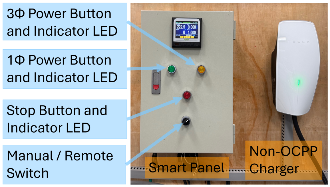
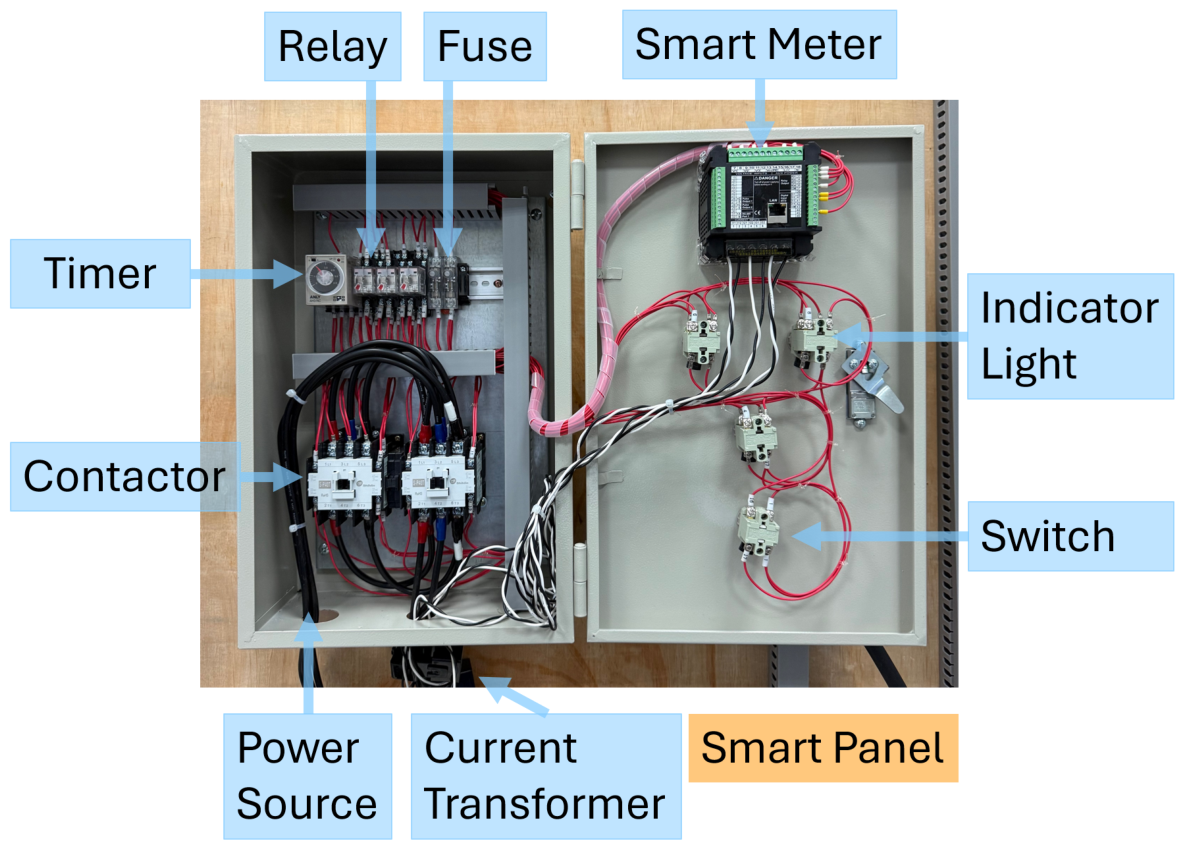
The complete Smart Panel design is shown in Figure 2, and the internal component layout is detailed in Figure 3.

Figure 2. External view of the Smart Distribution Panel showing the front-panel controls: a three-phase power button with an indicator LED, a single-phase power button with an indicator LED, an emergency-stop button with an indicator LED, and the manual/remote selector switch. The CPM-80 smart meter is mounted on top of the enclosure and provides a direct local readout of the 29 monitored electrical parameters.

Figure 2. External view of the Smart Distribution Panel showing the front-panel controls: a three-phase power button with an indicator LED, a single-phase power button with an indicator LED, an emergency-stop button with an indicator LED, and the manual/remote selector switch. The CPM-80 smart meter is mounted on top of the enclosure and provides a direct local readout of the 29 monitored electrical parameters.

Figure 3. Internal component layout of the Smart Distribution Panel (hardware photograph). Key components: the relay, fuse, CPM-80 smart meter, timer module, electromagnetic contactors, current transformers, power source terminals, indicator lights, and manual override switch. The corresponding electrical schematic and the bidirectional control/data flow are given in Figure 4 and Figure 5, respectively.

Figure 3. Internal component layout of the Smart Distribution Panel (hardware photograph). Key components: the relay, fuse, CPM-80 smart meter, timer module, electromagnetic contactors, current transformers, power source terminals, indicator lights, and manual override switch. The corresponding electrical schematic and the bidirectional control/data flow are given in Figure 4 and Figure 5, respectively.

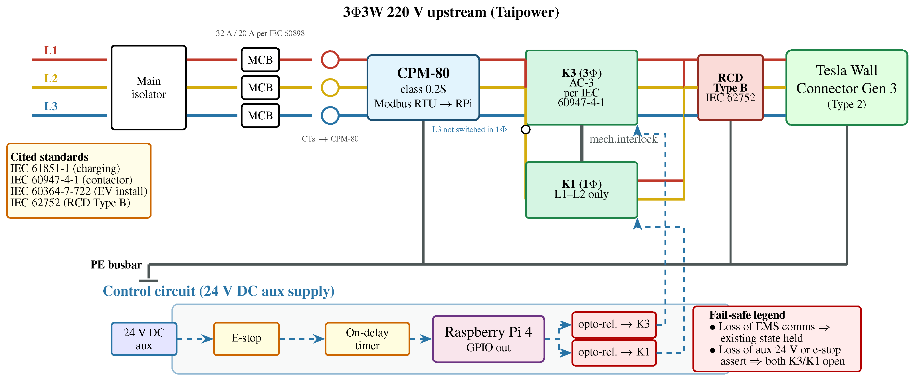
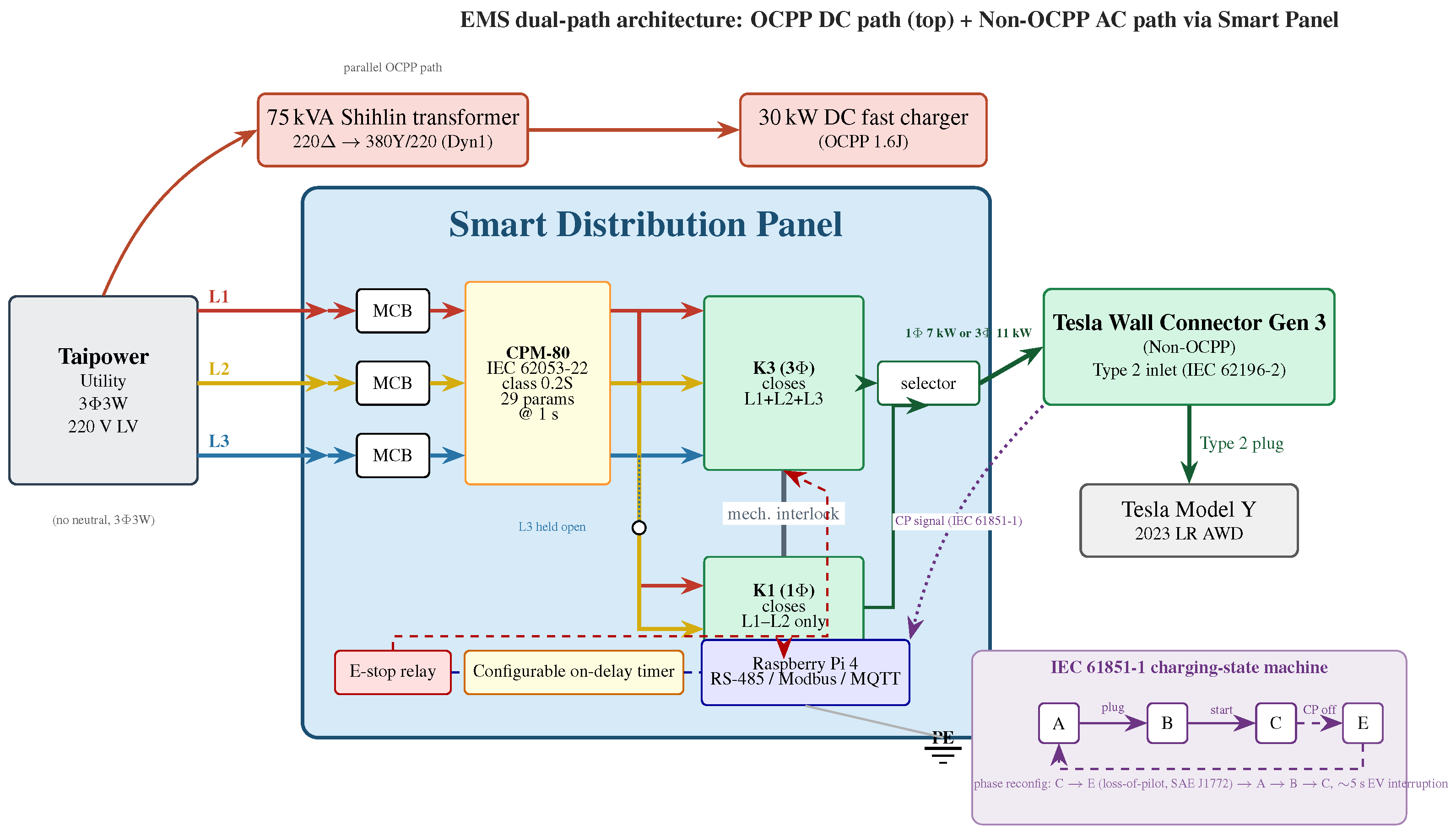
Figure 4. Smart Panel single-line and control schematic (solid lines: power path; dotted arrows: control path). Power path: the 3$\mathsf{\Phi }$3W 220 V upstream supply passes through a main isolator and per-phase MCBs into the CPM-80 measurement bus (CTs around each conductor; IEC 62053-22 class 0.2S [58]). Downstream of the CPM-80, K3 (three-phase contactor, AC-3 rated per IEC 60947-4-1 [59]) and K1 (single-phase contactor, switches L1–L2 only) are mechanically interlocked so that only one mode can be engaged at any time; in single-phase mode, L3 is held open. A Type B residual-current device (RCD; IEC 62752 [60] with the installation following IEC 60364-7-722 [61]) protects the EVSE-side branch before the Tesla Wall Connector Gen 3. The protective-earth (PE) busbar bonds all enclosure-side metalwork. Control path (dotted arrows): the 24 V auxiliary supply feeds the contactor coils through the e-stop relay and the configurable on-delay timer (mode-cycle protection); the Raspberry Pi 4 GPIO actuates opto-isolated relays that drive the coils through the same protection chain. Fail-safe legend: loss of EMS comms holds the existing state; loss of aux 24 V or any e-stop assertion drops both contactors to the open state.

Figure 4. Smart Panel single-line and control schematic (solid lines: power path; dotted arrows: control path). Power path: the 3$\mathsf{\Phi }$3W 220 V upstream supply passes through a main isolator and per-phase MCBs into the CPM-80 measurement bus (CTs around each conductor; IEC 62053-22 class 0.2S [58]). Downstream of the CPM-80, K3 (three-phase contactor, AC-3 rated per IEC 60947-4-1 [59]) and K1 (single-phase contactor, switches L1–L2 only) are mechanically interlocked so that only one mode can be engaged at any time; in single-phase mode, L3 is held open. A Type B residual-current device (RCD; IEC 62752 [60] with the installation following IEC 60364-7-722 [61]) protects the EVSE-side branch before the Tesla Wall Connector Gen 3. The protective-earth (PE) busbar bonds all enclosure-side metalwork. Control path (dotted arrows): the 24 V auxiliary supply feeds the contactor coils through the e-stop relay and the configurable on-delay timer (mode-cycle protection); the Raspberry Pi 4 GPIO actuates opto-isolated relays that drive the coils through the same protection chain. Fail-safe legend: loss of EMS comms holds the existing state; loss of aux 24 V or any e-stop assertion drops both contactors to the open state.

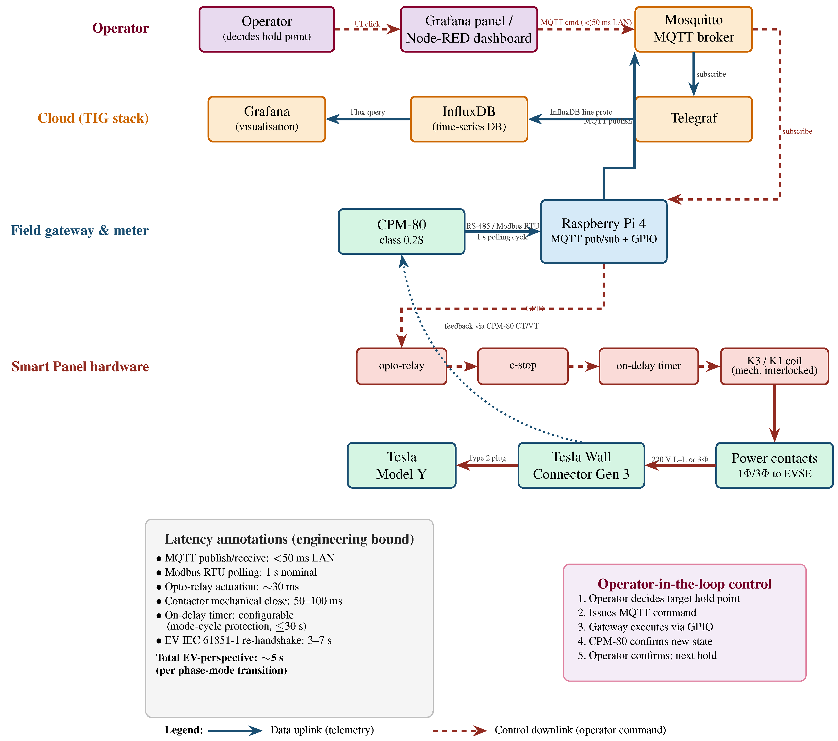
Figure 5. End-to-end data and control flow. Data uplink (solid arrows): CPM-80 → RS-485/Modbus RTU (1 s polling) → Raspberry Pi 4 → MQTT publish → Mosquitto broker → Telegraf → InfluxDB → Grafana operator view. Control downlink (dashed arrows): Operator → Grafana panel or Node-RED dashboard → MQTT command topic → Mosquitto broker → Raspberry Pi 4 (MQTT subscriber) → GPIO → opto-isolated relay → e-stop pass-through → configurable on-delay timer → contactor coil (K3 or K1, mechanically interlocked) → power contacts to the EVSE. The engineering latency bound (right) decomposes the total EV-perspective interruption per phase-mode transition into MQTT (<50 ms), Modbus (1 s polling), opto-relay actuation (∼30 ms), contactor mechanical close (50–100 ms), the on-delay timer (configurable mode-cycle protection), and the dominant IEC 61851-1 charging-state re-handshake (3–7 s observed at the CPM-80; total ∼5 s). The operator-in-the-loop control flow (lower-right inset) shows that the demonstrated capability is operator-commanded switching, not autonomous closed-loop demand response (which is explicitly future work).

Figure 5. End-to-end data and control flow. Data uplink (solid arrows): CPM-80 → RS-485/Modbus RTU (1 s polling) → Raspberry Pi 4 → MQTT publish → Mosquitto broker → Telegraf → InfluxDB → Grafana operator view. Control downlink (dashed arrows): Operator → Grafana panel or Node-RED dashboard → MQTT command topic → Mosquitto broker → Raspberry Pi 4 (MQTT subscriber) → GPIO → opto-isolated relay → e-stop pass-through → configurable on-delay timer → contactor coil (K3 or K1, mechanically interlocked) → power contacts to the EVSE. The engineering latency bound (right) decomposes the total EV-perspective interruption per phase-mode transition into MQTT (<50 ms), Modbus (1 s polling), opto-relay actuation (∼30 ms), contactor mechanical close (50–100 ms), the on-delay timer (configurable mode-cycle protection), and the dominant IEC 61851-1 charging-state re-handshake (3–7 s observed at the CPM-80; total ∼5 s). The operator-in-the-loop control flow (lower-right inset) shows that the demonstrated capability is operator-commanded switching, not autonomous closed-loop demand response (which is explicitly future work).

Phase-Reconfiguration Procedure

When the operator (or, in future autonomous control, which is not demonstrated here, the EMS) issues a $1\mathsf{\Phi }$/$3\mathsf{\Phi }$ mode-change command, the Smart Panel executes a deterministic sequence rather than performing an uninterrupted phase swap. The procedure intentionally interrupts EV charging for safety reasons; the total EV-perspective interruption observed at the CPM-80 during the experimental campaign was approximately five seconds per phase transition. The seven-step sequence is summarised in

Table 2. Phase-reconfiguration procedure (1$\mathsf{\Phi }$ ↔ 3$\mathsf{\Phi }$) executed by the Smart Panel. The total EV-perspective interruption observed at the CPM-80 was approximately 5 s per transition, dominated by the IEC 61851-1 charging-state re-handshake.

Step	Event	Approx. Duration
1	Operator/EMS issues mode-change command via MQTT to the Raspberry Pi gateway.	<1 s polling latency
2	Raspberry Pi GPIO de-energises the active contactor coil. CP (Control Pilot) line at the EVSE drops; EV transitions IEC 61851-1 State C → E (loss-of-pilot, SAE J1772 State E) → A (charging → no pilot → disconnected) [62].	∼0.5 s
3	Both contactors fully de-energised; mechanical interlock confirmed open; on-delay timer starts (mode-cycle protection).	0 s
4	Configurable on-delay timer holds both contactors open (mode-cycle protection element rated up to 30 s; deployed effective dead-time short enough that total EV-perspective interruption is ∼5 s; see Step 6).	≪5 s in deployed config
5	Target-mode contactor coil energised; mechanically interlocked alternate contactor remains locked open.	∼0.05 s
6	CP line at the EVSE re-asserts; EV runs IEC 61851-1 State A → B → C re-handshake; new charge current established.	∼5 s end-to-end from Step 2 to Step 6, EV perspective
7	CPM-80 confirms target-phase voltages/currents; status reported back via MQTT.	<1 s

.

• Interoperability scope.

The Smart Panel operates at the upstream electrical-supply boundary of the EVSE and performs no protocol-layer signalling. It does not assert or translate the Control Pilot (CP) or Proximity Pilot (PP) signals defined in IEC 61851-1 [62]. From the EVSE’s and the EV’s perspective, a phase reconfiguration commanded by the panel is observed as a brief supply removal that triggers the standard IEC 61851-1 state-machine transitions (Step 2 and Step 6 in Table 2). Because the panel is protocol-transparent in this sense, inter-EVSE interoperability and inter-EV interoperability rely on the IEC 61851-1 conformance of the connected equipment—they are not provided by the panel itself. The present work demonstrates the panel with one EVSE (Tesla Wall Connector Gen 3) and one EV (Tesla Model Y 2023 LR AWD); extension to other IEC 61851-1-compliant EVSE/EV pairs is conjectural and is stated as such in Section 4.1.

• Safety mechanisms.

The phase-reconfiguration procedure is protected by three independent mechanisms that prevent simultaneous engagement of incompatible phase configurations and prevent making-onto-fault: (i) mechanical interlock between the two contactors so that one cannot close while the other is closed; (ii) the configurable on-delay timer (mode-cycle protection) in series with both contactor coils so that even a software glitch issuing rapid mode toggles cannot energise either contactor within the dead-time; and (iii) mandatory e-stop pass-through of the coil supply so that any loss of control power or any e-stop assertion drops both contactors to the safe (open) state. A loss of EMS comms is treated as a passive condition: the existing contactor state is held, but no new switching command can be executed until comms restoration. The contactors are AC-3 rated per IEC 60947-4-1 [59]; the installation follows IEC 60364-7-722 for EV charging installations [61] with PE bonding at the panel ground bus per CNS-1500-style installation practice and Taipower’s LV service entrance specification.

• Limitations specific to the reconfiguration procedure.

The Smart Panel deliberately interrupts the EV charging session for ∼5 s during phase transitions; uninterrupted phase swapping is not supported and is not a goal of this design. The five-second interruption is acceptable for the operator-commanded site-level demand-management use case (operator decides when to demote a session at the granularity of minutes or longer) but is not a substitute for OCPP charge-profile negotiation (which can throttle current within a single session without interruption). The engineering bound on end-to-end command-to-resumption latency is reported in Section 3.4; no per-event success/failure record of the phase transitions themselves survives in the archived data (Section 4.1, L3).

2.3. Communication Architecture: Raspberry Pi 4 with RS-485 Protocol

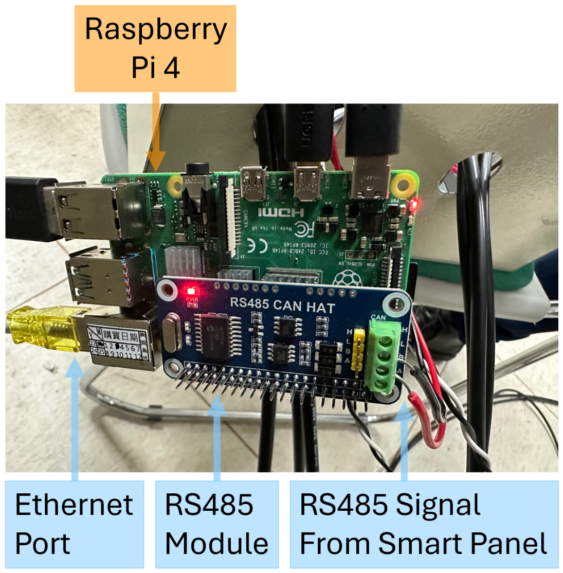
The Raspberry Pi 4 Model B serves as the field-level data acquisition gateway, bridging the Smart Panel hardware to the EMS software platform. Because the Pi does not natively support RS-485, an RS-485 CAN HAT on the 40-pin GPIO header provides the differential signalling needed in the electrically noisy panel environment; RS-485 was chosen as the physical layer for its multi-drop support, noise immunity, long reach (up to 1200 m at 100 kbps), and because it is the CPM-80’s Modbus RTU interface.

A Python (version 3.10) Modbus RTU master on the Pi polls the CPM-80 once per second, reading all 29 registers; each cycle is timestamped, packaged as an MQTT message, and published to the broker on the EMS server, where Telegraf writes it to InfluxDB. The Pi uses its built-in Gigabit Ethernet (preferred over Wi-Fi for industrial reliability), and the architecture is scalable: additional Smart Panels each add a Pi gateway publishing to the same broker and InfluxDB instance.

The Raspberry Pi 4 with the RS-485 CAN HAT module is shown in Figure 6.

2.4. Transformer for Three-Phase Power Conversion

The deployment site receives three-phase three-wire (3$\mathsf{\Phi }$3W) 220 V power from the utility distribution network. While this supply is adequate for the Non-OCPP chargers operating through the Smart Panel (which require 220 V single-phase or three-phase), the 30 kW OCPP-compliant DC fast charger requires a three-phase four-wire (3$\mathsf{\Phi }$4W) 380 V supply to meet its input power specifications.

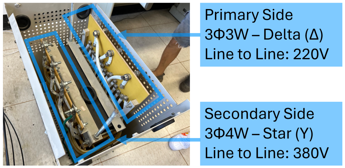
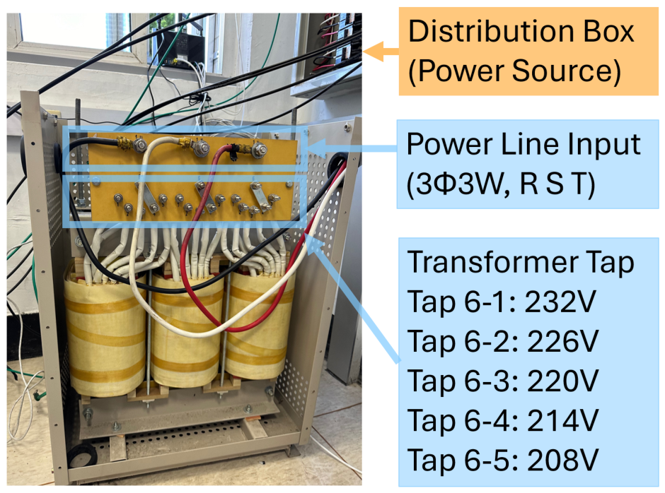
To address this requirement, a 75 kVA dry-type transformer is installed to perform the voltage and configuration conversion. The unit (Shihlin Electric model, CNS 13390, manufactured 2017-09; 290 kg; class-H insulation; AN cooling; serial PT4959) is configured with a delta ($\Delta$) primary winding connected to the incoming 3$\mathsf{\Phi }$3W 220 V supply and a star (Y) secondary winding providing the required 3$\mathsf{\Phi }$4W 380 V output with neutral, in vector group Dyn1 (30° phase shift, neutral grounded on the secondary). Per the nameplate, the rated short-circuit impedance at 75 °C is $Z=4.8\%$, the rated currents are 197 A on the primary $\Delta$ side and 114 A on the secondary Y side, and the primary winding offers five tap positions (208/214/220/226/232 V) for fine adjustment to the local utility voltage. The 75 kVA rating provides 2.5× headroom above the 30 kW charger requirement, accommodating inrush currents during charger startup and allowing for future expansion. Referred to the 220 V primary side, the transformer’s series impedance is $Z_{\mathrm{tx}}=(Z\%/100)·V_{\mathrm{LL}}^2/S=0.0310\mathsf{\Omega }$ per phase, dominantly reactive ($X/R\approx 8$ for a 75 kVA dry-type unit).

The installation includes standard protection devices (fuses, surge arresters) and a ventilated enclosure for heat dissipation under sustained high-power charging. The winding configuration is illustrated in Figure 7; the installed unit photo is in Figure 8.

2.5. Remote Monitoring Platform: Grafana, InfluxDB, and Telegraf

The software platform is built on the open-source TIG stack (Telegraf, InfluxDB, Grafana), widely used for time-series IoT monitoring [25]. Telegraf subscribes to the MQTT topics published by the Raspberry Pi 4 gateways, parses the JSON-formatted 29-parameter messages, and writes them to InfluxDB, a time-series database whose retention policies keep raw one-second data for recent periods and downsampled aggregates for long-term history. 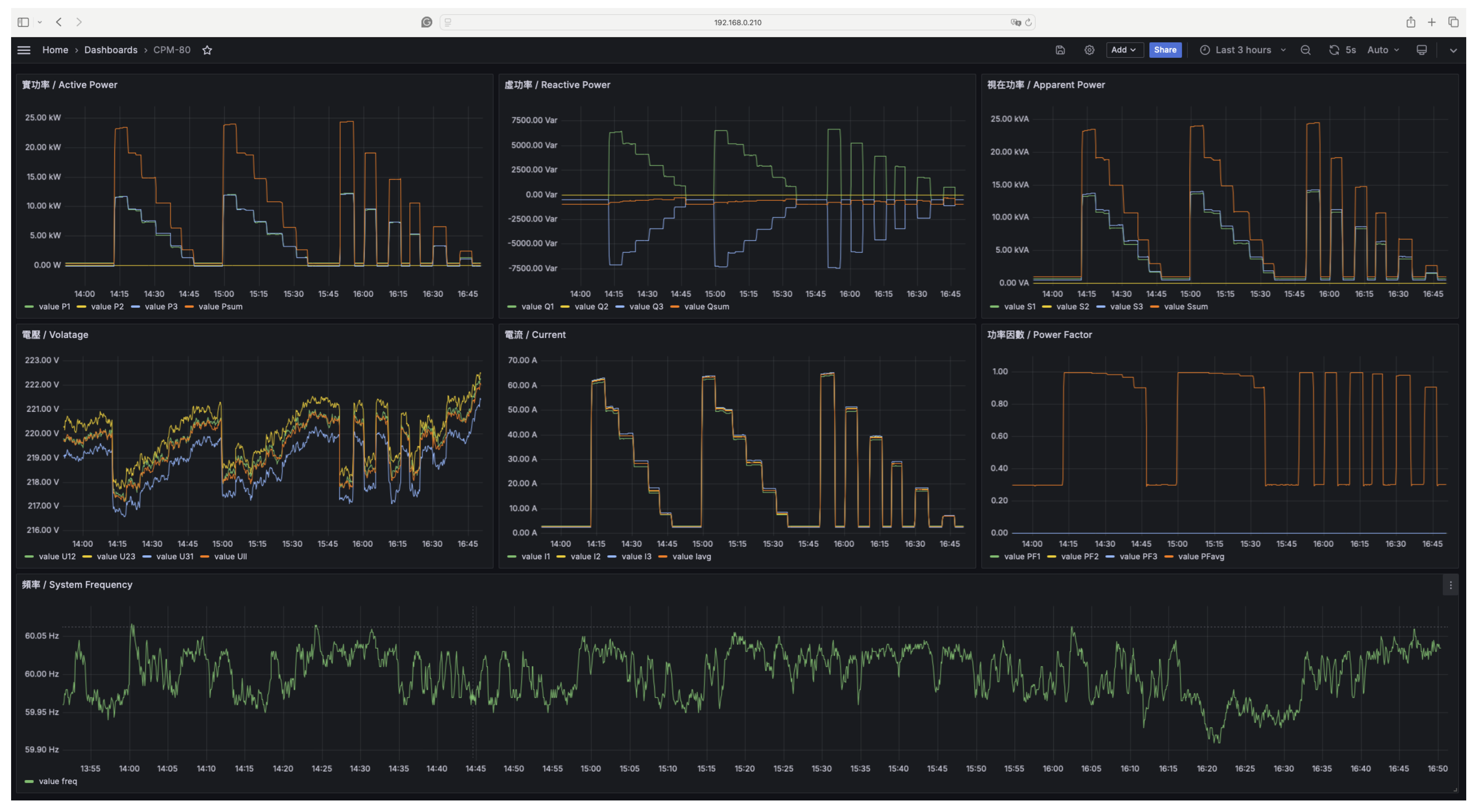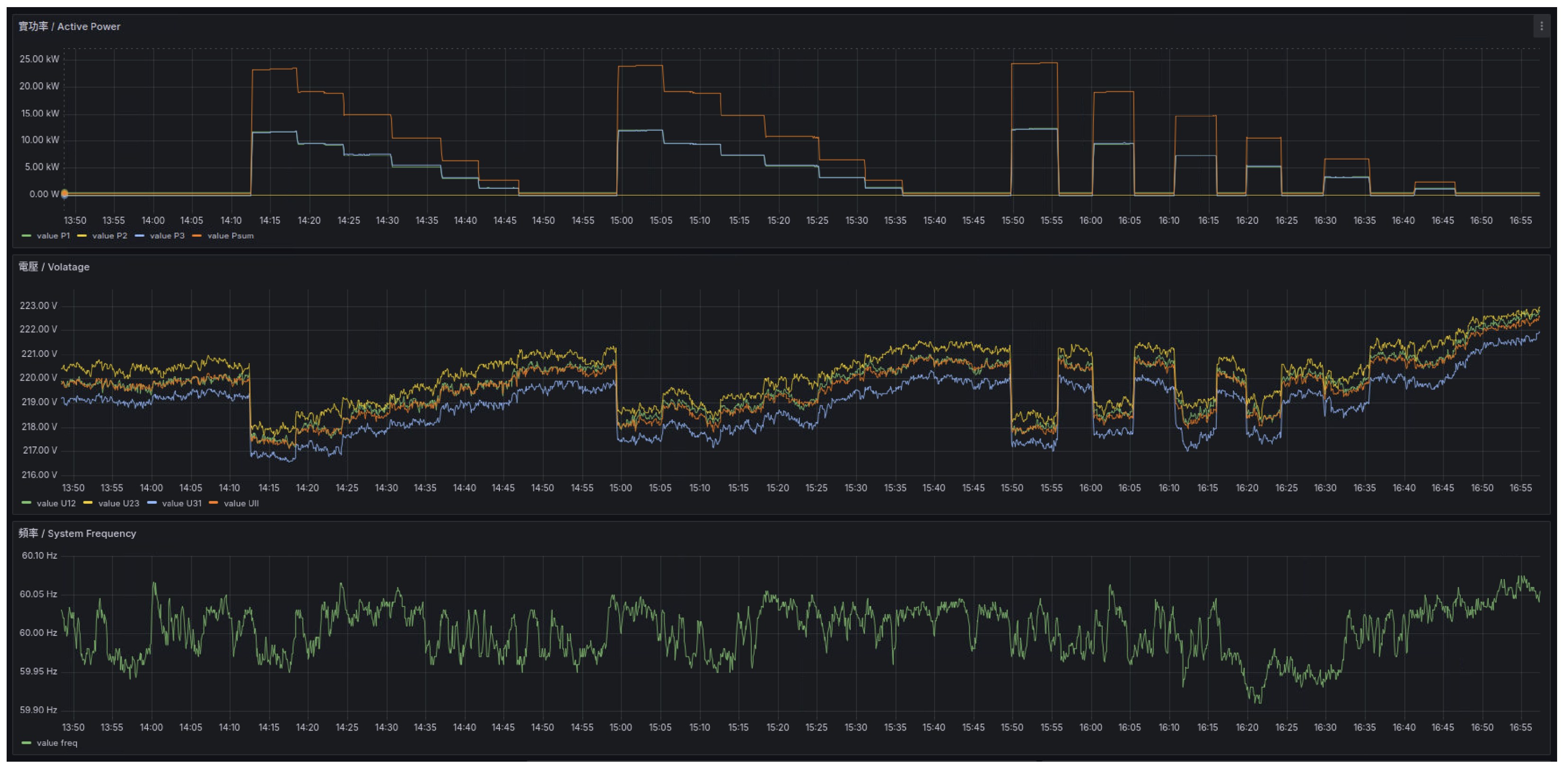Grafana provides browser-based dashboards that display per-phase voltages, currents, power, and power factors at a one-second resolution, with threshold-based alert rules and a historical time-range selector for post-event analysis; this historical record also serves as the LSTM training dataset (Section 2.6).

The monitoring architecture is shown in Figure 9; representative real-time and historical Grafana dashboards are shown in Figure 10 and Figure 11.

2.6. LSTM Model for Voltage Prediction

To complement the real-time monitoring capabilities of the Smart Panel, a Long Short-Term Memory (LSTM) neural network model is integrated as the principal analytical engine for residual-based anomaly detection. LSTM architectures have been successfully applied to smart grid anomaly-detection tasks, including electricity theft detection [63] and voltage state prediction [64], due to their ability to capture temporal dependencies in load-related variables through gating mechanisms [10,11].

Non-Autoregressive (Non-AR) Framing. The model adopts a non-autoregressive formulation: the target voltage $V_t$ is predicted from a sequence of load-side features only (power, currents, power factors, frequency, plus a cyclic time-of-day encoding), and the past values of V itself are deliberately not provided as input. This design is essential for residual-based anomaly detection: an autoregressive model that has access to past $V_{t-1},V_{t-2},\dots$ on a 1 Hz signal whose autocorrelation exceeds 0.99 will trivially predict ${\widehat{V}}_t\approx V_{t-1}$, masking any underlying physical fault that develops as a slow drift in V. The Non-AR formulation forces the model to learn the physical relationship $V=f$(load characteristics, time-of-day), so that a deviation from the learned conditional expectation—rather than from yesterday’s voltage—raises the anomaly flag. This is the same conceptual basis used by physical voltage-drop modelling ($\Delta V=I(R\cos \varphi +X\sin \varphi )$) but learned from data rather than imposed analytically.

Input Features. The model uses 12 load-side input features at each timestep: (1) Total_Power, (2) Avg_Current, (3) Avg_PF, (4–6) per-phase currents Current1, Current2, Current3, (7–9) per-phase power factors PF1, PF2, PF3, (10) frequency, and (11–12) a cyclic time-of-day encoding $\sin (2\pi ·h/24)$ and $\cos (2\pi ·h/24)$, where h is the local hour of the day. The cyclic time-of-day pair is included to absorb diurnal utility-side voltage variation (the ambient supply voltage at the deployment site naturally varies by 5–9 V across the day in response to upstream feeder loading external to this experiment), isolating the load-driven component of V for anomaly detection. Crucially, no past voltage value is included in the input feature set. The model is therefore not a forecaster in the autoregressive sense; it is a conditional-expectation estimator $\mathbb{E}[V_t\mid {\mathrm{load}}_{t-W:t},h_t]$ over a sliding window of length $W=20$ s.

Data Preprocessing. Raw data collected from the CPM-80 smart meter undergoes cleaning to remove communication errors, null values, and outlier readings caused by transient RS-485 bus collisions. Records with any missing or out-of-range fields are discarded. The cleaned data is filtered to charging-active periods (Total_Power > 2 kW, retaining 14,369 of 85,841 samples for the ML pipeline), then normalised using a MinMaxScaler fit on the training partition only. A sliding window of $W=20$ time steps (20 s at the one-second sampling rate) over the load-side features is used as the model input.

Model Architecture: The LSTM cell [65] processes sequential input through four interacting components—the forget gate, input gate, candidate cell state, and output gate—governed by the following equations:

$$f_t=\sigma (W_f·[h_{t-1},x_t]+b_f),$$

(1)

$$i_t=\sigma (W_i·[h_{t-1},x_t]+b_i),$$

(2)

$${\tilde{C}}_t=\tanh (W_C·[h_{t-1},x_t]+b_C),$$

(3)

$$C_t=f_t\odot C_{t-1}+i_t\odot {\tilde{C}}_t,$$

(4)

$$o_t=\sigma (W_o·[h_{t-1},x_t]+b_o),$$

(5)

$$h_t=o_t\odot \tanh \left(C_t\right),$$

(6)

where $x_t$ is the input vector at time step t, $h_{t-1}$ is the previous hidden state, $C_{t-1}$ is the previous cell state, ${\tilde{C}}_t$ is the candidate cell state, $\sigma$ denotes the sigmoid activation function, ⊙ represents element-wise multiplication, and W and b are the learnable weight matrices and bias vectors, respectively. The forget gate $f_t$ (Equation (1)) determines which information to discard from the cell state, the input gate $i_t$ (Equation (2)) controls which new information to store, and the candidate cell state ${\tilde{C}}_t$ (Equation (3)) generates new candidate values. The cell state $C_t$ (Equation (4)) is then updated by combining the forgotten previous state with the gated new candidates. Finally, the output gate $o_t$ (Equation (5)) regulates which information from the cell state is exposed as the hidden state $h_t$ (Equation (6)), which serves as both the layer output and the input to the next time step. This gating mechanism enables the LSTM to selectively retain relevant temporal patterns—such as voltage recovery dynamics after load changes—while discarding irrelevant noise.

The network consists of two stacked LSTM layers with 64 and 32 units, respectively, followed by a dense output layer with a single neuron for the voltage prediction. Dropout regularisation at 20% is applied between layers to prevent overfitting. The model is compiled with the Adam optimiser using a learning rate of 0.001 and trained with the mean squared error (MSE) as the loss function.

Training and Evaluation: The dataset is split into 80% training and 20% testing subsets using a chronological (non-shuffled) split to preserve the temporal ordering and prevent data leakage from future time steps into the training set. Early stopping with a patience of 10 epochs monitors the validation loss to prevent overfitting. Model performance is evaluated using the following standard regression metrics [63,64], where $y_i$ and ${\widehat{y}}_i$ denote the actual and predicted voltage values, $\overline{y}$ is the mean of the actual values, and N is the number of test samples:

$$\mathrm{RMSE}=\sqrt{{\displaystyle \frac{1}{N}}\sum _{i=1}^N{(y_i-{\widehat{y}}_i)}^2},$$

(7)

$$\mathrm{MAE}={\displaystyle \frac{1}{N}}{\displaystyle \sum _{i=1}^N}|y_i-{\widehat{y}}_i|,$$

(8)

$$R^2=1-{\displaystyle \frac{{\sum }_{i=1}^N{(y_i-{\widehat{y}}_i)}^2}{{\sum }_{i=1}^N{(y_i-\overline{y})}^2}}.$$

(9)

The RMSE (Equation (7)) penalises large deviations, the MAE (Equation (8)) provides an intuitive measure of average prediction error in volts, and $R^2$ (Equation (9)) quantifies the proportion of variance explained by the model. Two additional scale-independent metrics are also reported:

$$\mathrm{SMAPE}={\displaystyle \frac{100\%}{N}}{\displaystyle \sum _{i=1}^N}{\displaystyle \frac{|y_i-{\widehat{y}}_i|}{\left(\right|y_i|+|{\widehat{y}}_i\left|\right)/2}},$$

(10)

where SMAPE (Equation (10)) provides a percentage-based error measure that is symmetric in over- and under-prediction. All metrics are computed on the held-out test set. The trained model is deployed on the EMS server, where it processes incoming voltage data streams in near-real time.

The Non-AR LSTM is the principal analytical tool used in this work for residual-based anomaly detection on the high-resolution data stream enabled by the Smart Panel. We note that the load-only feature regression with cyclic time-of-day encoding adopted here is a standard formulation in physics-informed residual monitoring; the specific contribution is its application to panel-side voltage on a Non-OCPP charger and the quantitative anomaly-detection envelope reported in Section 3.3.3.

2.7. Experimental Equipment and Configuration

The experimental testbed is deployed at the EV charging facility of the Ming Chi University of Technology, New Taipei City, Taiwan (25.04° N, 121.45° E). The facility is connected to the utility grid through a building distribution panel that provides 3$\mathsf{\Phi }$3W 220 V of power. The cable layout from the building’s main distribution panel to the Smart Panel comprises a 50 m run of 22 mm² Cu XLPE feeder followed by a 2.5 m run of 5.5 mm² Cu XLPE; downstream of the Smart Panel, 2.5 m of 5.5 mm² Cu XLPE connects to the Tesla Wall Connector and 3 m of 5.5 mm² Cu XLPE connects to the 75 kVA $\Delta$-Y transformer (which then feeds the 30 kW DC OCPP charger via a separate 380 V three-phase output). All cable lengths and cross-sections were measured directly on site. The following equipment is installed and instrumented:

Non-OCPP Charger: A Tesla Wall Connector Gen 3 is installed as the primary Non-OCPP test subject. This charger supports both single-phase and three-phase input configurations, providing up to 7 kW (single-phase, 32 A at 220 V) and 11 kW (three-phase, 16 A per phase at 220 V). The charger does not support OCPP or any other standardised communication protocol; it operates autonomously once installed and cannot be remotely monitored or controlled without the Smart Panel.

OCPP Charger: A 30 kW DC fast charger with CCS1 and CCS2 connectors is installed on the transformer-fed 3$\mathsf{\Phi }$4W 380 V supply. This charger communicates via OCPP 1.6J over WebSocket, providing native integration with the EMS server.

Smart Distribution Panel: The custom-designed Smart Panel described in Section 2.2 is installed between the utility supply and the Tesla Wall Connector. The panel’s CPM-80 smart meter is configured for Modbus RTU communication at 9600 baud over RS-485.

Data Acquisition Gateway: A Raspberry Pi 4 Model B (4 GB RAM) with an RS-485 CAN HAT module is deployed adjacent to the Smart Panel, connected via a shielded twisted-pair RS-485 cable. The Raspberry Pi 4 runs Raspberry Pi OS with a custom Python data acquisition application.

EMS Server: A server running Ubuntu hosts the TIG stack (Telegraf 1.28, InfluxDB 2.7, Grafana 10.0) and provides the MQTT broker (Mosquitto) for data ingestion.

The complete hardware specifications are summarised in

Table 3. Hardware specifications of experimental equipment.

Component	Specification
Raspberry Pi 4	Model B, Broadcom BCM2711 (4× Cortex-A72 @ 1.5 GHz), 4 GB LPDDR4 RAM, Gigabit Ethernet, Raspberry Pi OS (Debian-based)
RS-485 CAN HAT	Waveshare RS485 CAN HAT, SN65HVD230 CAN transceiver, SP3485 RS-485 transceiver, 3.3 V logic
CPM-80 Smart Meter	ADTEK CPM-80 3$\mathsf{\Phi }$4W multifunction meter, voltage range 57.7–277 V (L-N)/100–480 V (L-L), accuracy class 0.2S per IEC 62053-22, Modbus RTU over RS-485, 9600 baud, 29 electrical parameters
Electromagnetic Contactors	Rated 40 A/220 VAC coil, mechanically interlocked, AC-3 duty cycle rated
Timer Module	Electronic on-delay timer, adjustable 1–60 s; commissioned-position maximum was 30 s, but the deployed dead-time during the experimental campaign was short enough that the EV’s IEC 61851-1 re-handshake (∼5 s, Section 2.2) dominated the per-transition interruption observed at the CPM-80
Current Transformers	Split-core type, ratio 100/5 A, accuracy class 0.5, compatible with CPM-80 CT inputs
Circuit Breakers	MCB, 32 A rated (single-phase path), 20 A rated (three-phase path), 10 kA breaking capacity
Tesla Wall Connector Gen 3	Hardware-rated up to 48 A/11.5 kW (single-phase) and 3 × 16 A/11 kW (three-phase); as deployed in this study, the single-phase mode is limited to 32 A/7 kW by the upstream MCB, while the three-phase mode runs at 3 × 16 A/11 kW. Type 2 connector (IEC 62196-2 [66]; the unit deployed in Taiwan ships with a Type 2 plug rather than the J3400/NACS variant used in the North American market)
OCPP DC Charger	30 kW, CCS1/CCS2, OCPP 1.6J over WebSocket, 3$\mathsf{\Phi }$4W 380 V input
Transformer	75 kVA dry-type (Shihlin Electric, 2017, CNS 13390 [67], class H, AN cooling); vector group Dyn1; $Z\%=4.8\%$ at 75 °C; rated currents 197 A primary/114 A secondary; 220 V $\Delta$ primary, 380Y/220 V secondary; 5-tap primary (208/214/220/226/232 V); 290 kg

.

2.8. Data Collection

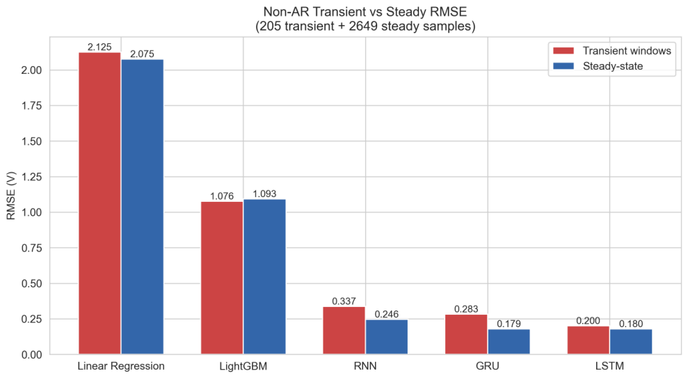
The CPM-80 smart meter measures 29 electrical parameters at one-second intervals, providing high-resolution temporal data suitable for both real-time monitoring and subsequent analysis. The one-second sampling rate was selected as a trade-off between temporal resolution and system resource constraints: it is fast enough to capture load-transition transients (which settle within 1–14 s, median 2 s, as quantified in Section 3.4) and to provide adequate input granularity for the LSTM model’s 20-step sliding window, while remaining within the Modbus RTU polling throughput achievable over RS-485 at 9600 baud (reading 29 registers requires approximately 350 ms per cycle, leaving sufficient margin within each one-second interval). The complete list of measured parameters is presented in

Table 4. Electrical parameters measured by CPM-80 smart meter.

Category	Parameters
Voltage	Avg_Voltage, Voltage1, Voltage2, Voltage3, Voltage12, Voltage23, Voltage31
Current	Avg_Current, Current1, Current2, Current3, Neutral_Current
Power	Total_Power, Power1, Power2, Power3, Total_Reactive_Power, Total_Apparent_Power
Power Factor	Avg_PF, PF1, PF2, PF3
Energy	Total_Energy, Import_Energy, Export_Energy
Other	Frequency, Demand_Power, Max_Demand_Power

.

Data is collected continuously during all test periods. Each data point is timestamped with millisecond precision using the Raspberry Pi 4’s Network Time Protocol (NTP)-synchronised system clock and stored in InfluxDB. The data collection system demonstrated high reliability during the experimental campaign, with a data capture rate of 99.35% over the 2024-02-22 acquisition day (85,841 of 86,400 one-second samples; the 0.65% shortfall is attributable to occasional RS-485 communication errors that are automatically recovered on the next polling cycle, as quantified in Section 3.4). The following data quality control measures are applied during acquisition and preprocessing:

• Communication error handling: If a Modbus RTU read fails (CRC error, timeout, or no response), the Raspberry Pi 4 retries up to two times within the same one-second polling cycle before discarding the sample and logging the error.
• Range validation: Each received parameter is checked against physically plausible bounds (e.g., voltage: 100–300 V; current: 0–100 A; power factor: 0–1.0). Out-of-range values are flagged and excluded from analysis.
• Continuity monitoring: Gaps in the time series exceeding 3 seconds are logged. Gaps shorter than 5 seconds are filled by linear interpolation for the LSTM training dataset; longer gaps are retained as session boundaries.

On 2024-02-22 (the primary analysis day), the system recorded 85,841 one-second samples spanning the full 24-h day, yielding a comprehensive dataset for analysis.

Charging session identification: Individual charging sessions are segmented from the continuous data stream using a threshold-based algorithm. A charging session is defined as a contiguous period during which Total_Power exceeds 0.5 kW (to exclude standby power draw) for at least 60 consecutive seconds. The session start is recorded at the first sample exceeding the threshold, and the session end is recorded when Total_Power drops below 0.5 kW for more than 30 consecutive seconds.

Multiple test days were conducted over the experimental period, with two primary datasets used for the analysis presented in this paper:

• 2024-02-22 (primary dataset): 85,841 one-second CPM-80 records spanning the full 24 h day (00:00:00–23:59:59 local time). Nine distinct charging sessions were identified by the $P>0.5$ kW segmentation rule; the 13:20–14:35 session (74.5 min) is the longest sustained high-load session and is used for the stepwise voltage impact analysis (Section 3.2).
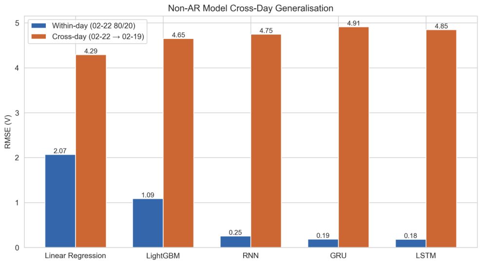
• 2024-02-19 (cross-day evaluation): 76,263 one-second records (00:00–21:15 local time), used as a held-out day for the cross-day generalisation experiment in Section 3.3.1.

Charging-active filter for the ML pipeline. For the Non-AR LSTM and baseline analyses (Section 3.3), the dataset is filtered to retain only charging-active samples by applying a power threshold of Total_Power > 2 kW. This focuses the predictive models on the charging-period dynamics that are operationally relevant for load management and power-quality monitoring; idle-state voltage patterns (when no EV is connected) are excluded from training and evaluation. After this filter, 14,369 of the 85,841 samples remain from 2024-02-22 for ML model fitting, which is sufficient for the 20-s sliding-window approach (yielding 14,349 examples). The implication is that the predictive models in this paper are valid only during periods of active charging; deployment for round-the-clock anomaly detection would require either retraining on idle-period data or enabling the detector exclusively during charging events.

Reproducibility. Sequence models are trained with eight random seeds {42, 7, 123, 11, 21, 31, 41, 51} and reported as the mean ± standard deviation across the eight seeds (Section 3.3). The full computational environment (software versions, GPU, per-model training times) and the archived data/code contents are detailed in Supplementary S5 and the Data Availability Statement.

In addition to infrastructure-side measurements from the CPM-80 smart meter, vehicle-side telemetry is collected through the Tessie cloud API for the test vehicle. The test EV is a Tesla Model Y, 2023 Long Range All-Wheel Drive (LR AWD), Taiwan market variant supplied with a Type 2 (IEC 62196-2 [66]) inlet; the onboard AC charger is rated up to 11.5 kW (single-phase, 48 A) or 11 kW (three-phase, 3 × 16 A) per Tesla published specifications. The vehicle was used as the only test EV throughout all charging sessions on the primary analysis day (2024-02-22) and the cross-day held-out day (2024-02-19); the single-vehicle scope is acknowledged as a limitation in Section 4.1. The Tesla Wall Connector Gen 3 firmware version active during the experimental campaign was not disclosed by Tesla to end users: the Tesla mobile app, the Wall Connector’s local web interface, and Tesla’s public documentation do not expose the running build identifier, and Tesla does not publish a public firmware changelog. The unit had been commissioned in 2023 and received Tesla’s automatic over-the-air (OTA) firmware updates through the experimental period without owner-visible version metadata; we acknowledge this as a transparency limitation of the Wall Connector Gen 3 ecosystem (Section 4.1). The Tessie data provides complementary parameters at 10-s intervals, including the battery state-of-charge (SOC), Charger Power as reported by the vehicle (this field reports the total power delivered to the vehicle through whichever charge port is active, whether AC or DC; during the 2024-02-22 13:20–14:35 stepwise session, this reported the OCPP DC fast-charger power; see Section 3.2), charger voltage, pack voltage, and battery temperature. During the 2024-02-22 experiment, the vehicle SOC progressed from 14% to approximately 90% across the nine charging sessions. This vehicle-side data enables cross-validation of the infrastructure-side power measurements recorded by the Smart Panel, confirming measurement consistency between the two independent data sources.

2.9. Test Scenarios

Two principal test scenarios are analysed quantitatively in this paper, both conducted with the Tesla Model Y 2023 LR AWD as the sole test vehicle on the Tesla Wall Connector Gen 3, and recorded continuously at the one-second sampling rate. The Smart Panel’s $1\mathsf{\Phi }$ and $3\mathsf{\Phi }$ operating modes were exercised during the broader experimental campaign, but they are not reported as separately analysed standalone scenarios: no dedicated $1\mathsf{\Phi }$ 7 kW or $3\mathsf{\Phi }$ 11 kW Wall Connector hold window exists in the archived record that could be cleanly separated at the data level, and the 13:20–14:35 stepwise sweep itself ran entirely on the DC-charger path with the Wall Connector idle (Scenario 1 below). To ensure that reported voltage levels reflect quasi-steady-state conditions rather than transient artefacts, all per-hold values are computed as the mean over a minimum stabilisation window of 60 s after the load reaches its target level.

Scenario 1: Stepwise Load Reduction (Primary Evidence). Conducted on 2024-02-22, this scenario characterises the voltage–power relationship at the Smart Panel point of common coupling (PCC) bus across the operating range of the deployed Smart Panel + 30 kW OCPP DC charger + Tesla Wall Connector + site-base-load ensemble. Starting from the maximum in-session load (approximately 28–30 kW), the operator-commanded discrete down-steps: 28 kW → 24 kW → 20 kW → 16 kW → 12 kW → 8 kW → 4 kW. Each target is held long enough to retain at least one 60-s post-stabilisation window, and most targets contain 9–11 such windows. Vehicle-side telemetry from the Tessie cloud API for the test Tesla Model Y (Section 2.8; per-hold breakdown in Section 3.2) confirms that the test EV was charged through the OCPP DC fast-charger path during this session, with the Non-OCPP Wall Connector AC path idle for the 75 min window; the load ladder was therefore implemented as a DC-charger current-limit demotion sequence, not as a Wall Connector $3\mathsf{\Phi }\to 1\mathsf{\Phi }$ demotion. The Wall Connector $3\mathsf{\Phi }\leftrightarrow 1\mathsf{\Phi }$ phase-reconfiguration capability and its ∼5 s EV-perspective interruption are documented separately in Section 2.2 and Table 2. Scenario 1 is therefore a characterisation of the overall site PCC under controllable load, in which the Smart Panel serves as the measurement instrument; it is not a direct evaluation of the Smart Panel’s Non-OCPP reconfiguration path, which was idle throughout the session. This scenario provides the primary evidence for the in-session voltage–load slope analysis (Section 3.2); fully autonomous closed-loop demand response operation is reserved as future work.

Scenario 2: Cross-Day Held-Out Check (2024-02-19). The Non-AR LSTM and the baseline models trained on the 2024-02-22 dataset are evaluated on the 2024-02-19 held-out day (76,263 one-second records) for within-site day-to-day generalisation assessment (Section 3.3.1). This is not cross-site or cross-charger generalisation evidence; it is a single held-out day at the same site with the same equipment.

It should be noted that because the experiments are conducted at an operational university facility connected to the live utility grid, the baseline voltage is subject to natural fluctuations caused by other building loads and upstream grid conditions. These background variations are on the order of ±1 V and represent a source of measurement uncertainty that is inherent to field-deployed (as opposed to laboratory) testing. Upstream/PCC utility-side voltage is not directly logged in this campaign; this is treated as an explicit limitation in Section 4.1.

3. Results

3.1. Voltage Impact Under Different Load Conditions

The voltage behaviour of the distribution system under various EV charging loads is characterised using data collected from the CPM-80 smart meter through the Smart Panel. Throughout Section 3.1 and Section 3.2, the quantity being characterised is the site-level PCC bus under controllable (DC-charger-driven) load; the Smart Panel’s role in these sections is that of the measurement instrument providing the one-second observability, not that of the device under test—its Non-OCPP reconfiguration path was idle during the stepwise session (Section 2.9). The 2024-02-22 dataset (85,841 one-second samples spanning the full 24 h day) shows that the utility supply voltage at the PCC bus varies naturally by 1–2% across the day in response to feeder loading external to this experiment: the lowest-load 5% of samples (when the local charging load is below 295 W, $n=5617$) average $V=219.62$ V ($\sigma =0.45$ V), whereas during the 13:20–14:35 stepwise session, the local reference voltage at the 4 kW hold is $V=224.26$ V ($\sigma =0.16$ V). Time-of-day utility-side variation therefore exceeds the cleanest in-session voltage drop induced by EV charging at this site, so we report the voltage impact as intra-session differences rather than relative to a daily fixed baseline.

Table 5. Observed voltage levels at the PCC Bus, 2024-02-22 (intra-session and daily references).

Condition	N Samples	V Mean (V)	$\mathit{\sigma }$ (V)
Daily low-load reference a	5617	219.62	0.45
30 kW DC fast charger active b	3114	222.12	0.74
Stepwise 4 kW hold (session-local reference)	∼660	224.26	0.16
Stepwise 28 kW hold (highest in-session load)	∼720	220.93	0.17

^a Lowest 5% of one-second samples by Total_Power (P ≤ 295 W). ^b All samples with 28 kW ≤ P ≤ 30.5 kW; spans the 09:37–10:39 and 13:20–14:35 sessions.

summarises the principal observed voltage levels and their sample counts; the stepwise hold-by-hold data is in

Table 6. Stepwise load reduction results from the 2024-02-22 13:20–14:35 session (74.5 min).

Step	Target P	60 s Holds	Avg. V	$\mathit{\sigma }$	$\mathbf{\Delta }\mathit{V}$ from 4 kW Reference
	(kW)	$\mathbf{N}$	(V)	(V)	(V)
1	28	12	220.93	0.17	−3.33
2	24	8	221.17	0.14	−3.09
3	20	8	221.91	0.10	−2.35
4	16	9	222.37	0.12	−1.89
5	12	8	223.13	0.15	−1.13
6	8	9	223.78	0.23	−0.48
7	4	11	224.26	0.16	0 (reference)

N = number of 60-s windows aggregated within the hold band (±0.5 kW around the target). Each value is the mean voltage within a single 60 s window; $\sigma$ is the standard deviation of voltage within the same window. Per-step sample sizes are $N\times 60\approx 480$–720 one-second samples.

.

The intra-session 4 kW → 28 kW drop within the 13:20–14:35 stepwise experiment is therefore $224.26-220.93=3.33\mathrm{V}$, equivalent to 1.49% of the 4 kW reference level. The 28 kW measurement is consistent across both the morning (09:37–10:39, 30 kW via the OCPP DC charger) and afternoon (13:20–14:35, likewise via the OCPP DC charger with the Wall Connector idle) sessions. Note that the daily low-load reference (219.62 V) is approximately 4.64 V lower than the in-session 4 kW reference (224.26 V); this is attributable to natural utility-side voltage variation between the early-morning low-demand period and the midday charging window, not to the local charging load.

Dedicated 7 kW single-phase and 11 kW three-phase Wall Connector standalone test windows were not separately captured in the 2024-02-22 data record: vehicle-side telemetry from the Tessie cloud API for the test Tesla Model Y (Table 7 in Section 3.2) confirms that the Wall Connector AC path was idle during the 13:20–14:35 stepwise session (the load ladder was a DC-charger current-limit demotion sequence, not a Wall Connector $3\mathsf{\Phi }\to 1\mathsf{\Phi }$ demotion). The Wall Connector $1\mathsf{\Phi }\leftrightarrow 3\mathsf{\Phi }$ phase-reconfiguration capability and its ∼5 s EV-perspective interruption are documented from independent operational events in Section 2.2 and Table 2, not from this stepwise dataset. Below we therefore report only the conditions for which a clean, sustained measurement window exists in the 2024-02-22 record: the 4 kW and 28 kW endpoints of the stepwise session, plus the daily low-load reference and the 30 kW DC fast-charger active periods. The full hold-by-hold stepwise data is in Table 6.

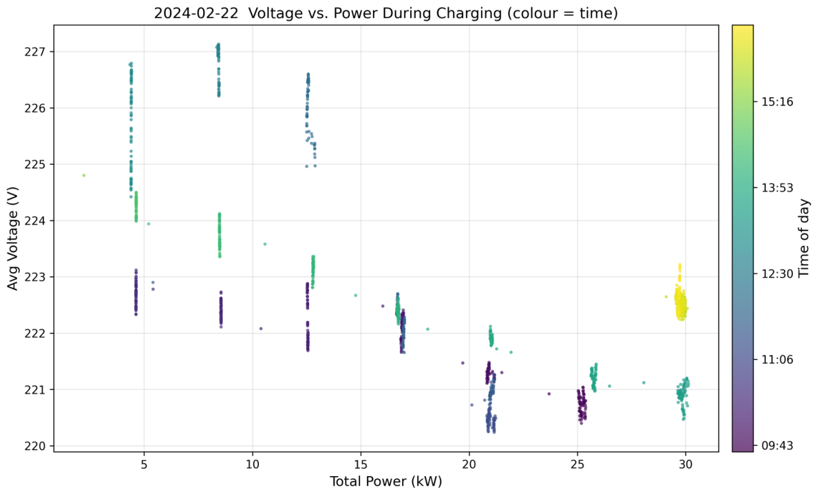
Three-phase imbalance. The three-phase voltage data (Voltage1, Voltage2, Voltage3) collected by the Smart Panel shows phase-to-phase voltage imbalance under load, typically below 0.5 V at low load and up to 1 V at the 28 kW step, attributable to inherent asymmetries in the distribution network impedance and unequal loading from other building loads on the same feeder. The voltage-vs-power scatter for the 13:20–14:35 stepwise sweep is illustrated in Figure 12.

3.2. Stepwise Load Reduction Analysis: A Site-Level PCC Characterisation

The stepwise load reduction experiment was conducted on 2024-02-22 between 13:20 and 14:35 (74.5 min total). The full 24 h dataset contains nine distinct charging sessions; the longest sustained high-load session (the 13:20–14:35 window) is the one used here for stepwise analysis because it contains all seven hold levels with at least nine 60 s stable windows each. Vehicle-side telemetry from the Tessie cloud API (Section 2.8, Table 7) confirms that during this 75 min window the test EV was charged through the OCPP DC fast-charger path, with the Non-OCPP Wall Connector AC path idle. Starting from the highest in-session load of approximately 28–30 kW, the total charging power was reduced through discrete operator-commanded steps: the DC charger’s output current was progressively reduced via OCPP current-limiting commands issued from the EMS server (the Wall Connector $3\mathsf{\Phi }\to 1\mathsf{\Phi }$ reconfiguration capability and its ∼5 s EV-perspective interruption are documented in Section 2.2 from independent operational events, not this stepwise session). Each intermediate power level was maintained long enough for at least one 60-s stable window to be retained from the data record. We post hoc identify “stable” windows as 60-s intervals where the total charging power remained within ±0.5 kW of the operator’s nominal target. The mean and standard deviation of the line voltage within each such window are then aggregated into the per-step values reported in Table 6. Note that the ±0.5 kW band is applied within the 13:20–14:35 session only. Running the same selection across the full 24 h record would return many more samples for low-power steps (because idle periods often dwell near 4–8 kW) and few or no samples for the 12–28 kW high-load steps, which only occur in this single session. All per-step aggregations and the headline regression therefore refer specifically to the in-session windows of this 75 min experiment.

Table 7. Per-hold PCC-total vs. vehicle-side DC power cross-check during the 2024-02-22 stepwise session (13:20–14:35). PCC values are CPM-80 means over the listed hold window; Vehicle (Tessie) is the vehicle-side Charger Power reported by the Tessie cloud API for the test Tesla Model Y; residual = PCC − vehicle. Throughout this 75 min window the Non-OCPP Wall Connector AC path was idle (Tessie Charger Voltage ≈ 2 V sensor zero and Charger Phases empty, both consistent with DC-mode charging through the OCPP path). There is therefore no AC/DC split to report: the table is a PCC-total versus vehicle-side DC-power cross-check, not an AC/DC apportionment. Tessie 10 s telemetry coverage begins at 13:35:47, so Hold 1 has no per-second vehicle reference and is instead corroborated by battery state-of-charge (footnote †).

Step	Window	PCC	${\mathit{V}}_{\mathbf{PCC}}$	Vehicle (Tessie)	Residual
	(hh:mm)	(kW)	(V)	(kW)	(kW)
1	13:21–13:33	29.85	220.93	— †	— †
2	13:34–13:42	25.75	221.17	23.00	2.75
3	13:44–13:52	21.02	221.91	20.00	1.02
4	13:53–14:02	16.74	222.37	15.07	1.67
5	14:04–14:12	12.80	223.13	12.00	0.80
6	14:14–14:23	8.48	223.78	8.00	0.48
7	14:24–14:35	4.64	224.26	4.04	0.60

^† The Tessie 10 s telemetry export begins at 13:35:47, so Hold 1 (13:21–13:33) has no per-second vehicle-side power. Two independent lines of evidence corroborate it: (i) the Hold-1 PCC total of 29.85 kW exceeds the Wall Connector $3\mathsf{\Phi }$ rating (11 kW) by ∼19 kW, so the DC charger via the transformer is necessarily the dominant load; and (ii) the vehicle battery state-of-charge was 46% at 13:15 (immediately before the hold) and 54% at 13:35 (immediately after), and since state-of-charge can only rise through charging, this ∼8-percentage-point increase confirms that the test EV was charging at high power during this hold. The lack of per-second telemetry here is not specific to Hold 1: the cloud telemetry service polls intermittently and had six >10 min gaps across the day, Hold 1 coinciding with one, whereas Holds 2–7 lie within the continuous window from 13:35:47. Residuals (0.5–2.8 kW) combine site house base load (lighting, building loads, ∼1 kW), 75 kVA transformer no-load plus load losses scaling with through-power (∼2–5% at primary side), and AC-side cable losses between PCC and the transformer primary; they are not separately decomposed in this campaign and are reported as the aggregated residual.

Table 7. Per-hold PCC-total vs. vehicle-side DC power cross-check during the 2024-02-22 stepwise session (13:20–14:35). PCC values are CPM-80 means over the listed hold window; Vehicle (Tessie) is the vehicle-side Charger Power reported by the Tessie cloud API for the test Tesla Model Y; residual = PCC − vehicle. Throughout this 75 min window the Non-OCPP Wall Connector AC path was idle (Tessie Charger Voltage ≈ 2 V sensor zero and Charger Phases empty, both consistent with DC-mode charging through the OCPP path). There is therefore no AC/DC split to report: the table is a PCC-total versus vehicle-side DC-power cross-check, not an AC/DC apportionment. Tessie 10 s telemetry coverage begins at 13:35:47, so Hold 1 has no per-second vehicle reference and is instead corroborated by battery state-of-charge (footnote †).

Step	Window	PCC	${\mathit{V}}_{\mathbf{PCC}}$	Vehicle (Tessie)	Residual
	(hh:mm)	(kW)	(V)	(kW)	(kW)
1	13:21–13:33	29.85	220.93	— †	— †
2	13:34–13:42	25.75	221.17	23.00	2.75
3	13:44–13:52	21.02	221.91	20.00	1.02
4	13:53–14:02	16.74	222.37	15.07	1.67
5	14:04–14:12	12.80	223.13	12.00	0.80
6	14:14–14:23	8.48	223.78	8.00	0.48
7	14:24–14:35	4.64	224.26	4.04	0.60

^† The Tessie 10 s telemetry export begins at 13:35:47, so Hold 1 (13:21–13:33) has no per-second vehicle-side power. Two independent lines of evidence corroborate it: (i) the Hold-1 PCC total of 29.85 kW exceeds the Wall Connector $3\mathsf{\Phi }$ rating (11 kW) by ∼19 kW, so the DC charger via the transformer is necessarily the dominant load; and (ii) the vehicle battery state-of-charge was 46% at 13:15 (immediately before the hold) and 54% at 13:35 (immediately after), and since state-of-charge can only rise through charging, this ∼8-percentage-point increase confirms that the test EV was charging at high power during this hold. The lack of per-second telemetry here is not specific to Hold 1: the cloud telemetry service polls intermittently and had six >10 min gaps across the day, Hold 1 coinciding with one, whereas Holds 2–7 lie within the continuous window from 13:35:47. Residuals (0.5–2.8 kW) combine site house base load (lighting, building loads, ∼1 kW), 75 kVA transformer no-load plus load losses scaling with through-power (∼2–5% at primary side), and AC-side cable losses between PCC and the transformer primary; they are not separately decomposed in this campaign and are reported as the aggregated residual.

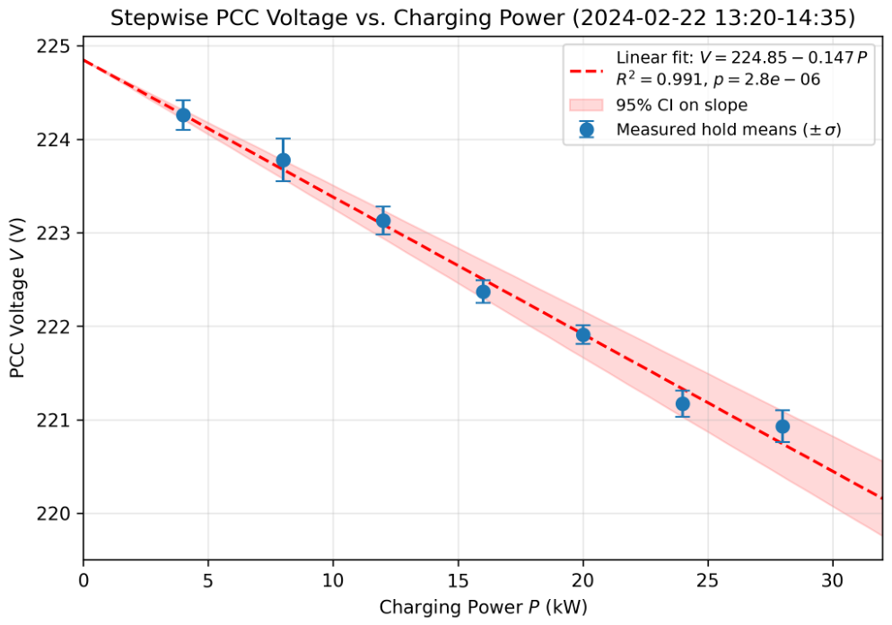
Statistical analysis of the voltage–power relationship. A linear regression of voltage against charging power across the seven hold points in Table 6 yields a strongly significant linear fit:

$$V=224.85-0.147P,R^2=0.991,p=2.8\times {10}^{-6},$$

(11)

where V is the in-session PCC voltage in volts and P is the total charging power in kilowatts. The slope is $|dV/dP|=0.147\pm 0.013$ V/kW (slope standard error 0.0064 V/kW, degrees of freedom five), or equivalently a recovery rate of approximately $1\mathrm{V}$ per $6.8\mathrm{kW}$ of load reduction. The 95% confidence interval $[0.134,0.159]$ V/kW excludes zero ($p=2.8\times {10}^{-6}$), confirming statistical significance. The visualisation of this regression, with the per-step measurements and the linear-fit 95% confidence band, is provided in Figure 13.

Robustness to the highest-load anchor. Hold 1 (28 kW) is the highest-leverage point of the regression and is the only hold without per-second vehicle-side telemetry (Table 7). A leave-one-out check shows that the slope remains in the range 0.143–0.156 V/kW when any single hold is removed (removing Hold 1 specifically gives 0.156 V/kW, $R^2=0.996$), so the headline sensitivity does not hinge on this single point. Hold 1 is independently corroborated by the vehicle battery state-of-charge, which was 46% at 13:15 (immediately before the hold) and 54% at 13:35 (immediately after), as recorded by the vehicle’s cloud telemetry (Table 7, footnote †); because state-of-charge can only increase through charging, this ∼8-percentage-point rise confirms that the test EV was the dominant high-power load during this hold. The absence of per-second telemetry at Hold 1 is not specific to that hold: the vehicle’s cloud telemetry service polls the manufacturer API intermittently and exhibited six coverage gaps exceeding ten minutes across the 2024-02-22 day, Hold 1 coinciding with one of them, whereas Holds 2–7 fell within the continuous afternoon telemetry window beginning at 13:35:47. The continuous one-second panel-side metering captured the Hold 1 charging that the intermittent cloud telemetry missed—a concrete instance of the observability gap that motivates the Smart Panel.

Statistical resolvability of the per-step voltage drops. The within-window standard deviations are small (0.10–0.23 V), so the seven hold means are clearly separated within this single 75 min session. The empirical regression slope (95% CI [0.134, 0.159] V/kW) excludes zero at $p=2.8\times {10}^{-6}$. This inference should be interpreted as an in-session statistical result: it does not include full instrument-calibration uncertainty, autocorrelation among one-second samples, or unmeasured upstream utility-voltage drift.

OpenDSS bounded sanity check (parameter-free upper bound). To check whether the empirical slope reported in Equation (11) is consistent with the physics of the deployed distribution network, a parameter-free power-systems simulation was performed using OpenDSS [68]. All impedance values used in the simulation come from direct on-site measurement (cable lengths and cross-sections) or from the transformer nameplate; no parameter is fitted to the measured voltage data. We frame this as a bounded sanity check rather than a validation: because the upstream/PCC utility-side voltage was not separately logged during the campaign (a limitation we acknowledge in Section 4.1), the OpenDSS result yields the cable-and-transformer-impedance upper bound on the slope, not the slope that should match the measurement.

The deployment topology was modelled as follows: a three-phase 220 V utility source feeds a 50 m run of 22 mm² copper XLPE cable (campus EV-facility feeder), then a 2.5 m run of 5.5 mm² Cu XLPE to the Smart Panel (which contains the CPM-80 measurement bus, designated as the point-of-common-coupling, PCC). From the PCC, two parallel paths are modelled: (i) a 2.5 m × 5.5 mm² Cu XLPE branch to the Tesla Wall Connector (Non-OCPP, up to 11 kW load); and (ii) a 3 m × 5.5 mm² Cu XLPE branch to the 75 kVA $\Delta$-Y transformer (Dyn1, $Z\%=4.8\%$ at 75 °C), which feeds the 30 kW DC OCPP charger on its 380 V secondary. Cable resistances were computed from copper resistivity at 75 °C operating temperature ($\rho \approx 0.0210\mathsf{\Omega }·{\mathrm{mm}}^2/\mathrm{m}$, derived from ${\rho }_{\mathrm{Cu}}$(20 °C) = 0.01724 with temperature coefficient $\alpha =0.00393{\mathrm{K}}^{-1}$ per IEC 60228), giving $R\approx 0.954\mathsf{\Omega }/\mathrm{km}$ for 22 mm² and $R\approx 3.81\mathsf{\Omega }/\mathrm{km}$ for 5.5 mm²; cable reactance was set to 0.09–0.10 $\mathsf{\Omega }/\mathrm{km}$ for low-voltage XLPE. The transformer’s series impedance referred to the 220 V primary side is $\left|Z_{\mathrm{tx}}\right|=0.0310\mathsf{\Omega }$/phase, calculated directly from the nameplate $Z\%$ and rated kVA.

The transformer’s $X/R$ ratio was not measured directly. Published values for small dry-type units span a wide range: GE 75 kVA QHT $X/R\approx 0.84$, Square-D 75 kVA $X/R\approx 1.19$, with manufacturer specifications typically in the 0.5–2 band; a few designs reach 5–8. We therefore performed a sensitivity sweep over $X/R\in \{0.5,0.84,1.5,3.0,8.0\}$ rather than commit to a single point estimate.

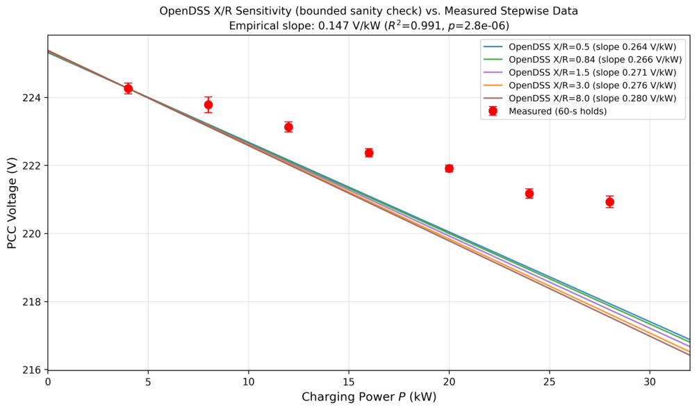
The OpenDSS bounded sanity check predicts a voltage–power slope in the range 0.26–0.28 V/kW across the swept $X/R$ values; the measured slope of $0.147\pm 0.013$ V/kW (Equation (11)) therefore lies at approximately 55% of this upper bound. Two important caveats apply when interpreting this gap.

Ensemble effective sensitivity and per-hold cross-check. The PCC bus monitored by the CPM-80 aggregates the two electrically distinct charging paths supported by the Smart Panel architecture: the OCPP DC fast charger (fed through the 75 kVA $\Delta$-Y step-up transformer described in Section 2.4) and the Non-OCPP Tesla Wall Connector Gen 3 (connected directly to the 220 V three-phase supply). For the 13:20–14:35 session reported here, vehicle-side telemetry from the Tessie cloud API for the test Tesla Model Y confirms that the EV was charged via the OCPP DC path: across 357 vehicle-side data samples (10 s cadence, 13:35:47–14:35:17) the Tessie-reported Charger Voltage reads ∼2 V and Charger Phases is empty, both consistent with DC-charging mode (the Wall Connector AC path was idle for this 75 min window, so there is no AC/DC split—the comparison is a PCC-total versus vehicle-side DC cross-check). The per-hold cross-check is shown in Table 7: Tessie-reported vehicle power tracks the PCC ladder to within 0.5–2.8 kW, with the residual consistent with the site’s house base load. The 0.147 V/kW slope is therefore best read as the ensemble effective sensitivity of the PCC bus to combined heterogeneous loads (the DC charger plus uncoordinated site base) under the operational mix that occurred during this session, not as a single-path physical property of one charger.

Why the empirical slope is lower than the OpenDSS upper bound. The OpenDSS curves in Figure 14 are a conservative upper bound on the predicted sensitivity (0.26–0.28 V/kW) constructed from the nameplate transformer impedance ($Z\%=4.8\%$ at 75 °C) and the cable cross-section/length at the upper-end operating-temperature assumption. The empirical 0.147 V/kW being lower than the upper bound is therefore consistent with the actual path impedance being smaller than the upper-bound model. Plausible mechanisms include: (i) the actual cable operating temperature being below the 75 °C reference (the resistance temperature coefficient $\alpha =0.00393{\mathrm{K}}^{-1}$ per IEC 60228 means a 40 °C operating temperature would lower cable resistance by ∼14% relative to 75 °C); (ii) the actual transformer $X/R$ ratio sitting at the low end of the swept band $\{0.5,0.84,1.5,3.0,8.0\}$, where the predicted slope is closer to 0.26 than to 0.28 V/kW; and (iii) upstream voltage regulation (utility tap-changer action or stiff source impedance at the LV service entrance) partially compensating the load-side voltage drop within the 75 min session. Our single-point CPM-80 instrumentation at the PCC cannot decompose these factors. Direct $X/R$ characterisation of the on-site transformer (via short-circuit or LCR-meter test) plus simultaneous upstream voltage logging would be required to attribute the gap precisely; we identify both as key validation enhancements for future deployments rather than reaching a definitive single-cause attribution from the current dataset. The full $X/R$ sweep is shown in Figure 14.

The data reveals a clear and approximately linear relationship between total charging power and PCC voltage within the 13:20–14:35 session. At the highest in-session load (28 kW), the voltage settles at 220.93 V; at the lowest (4 kW), 224.26 V; the in-session drop of 3.33 V over a 24 kW span corresponds to the 0.147 V/kW slope reported in Equation (11). We are explicit that this slope describes the in-session relationship at the PCC bus and is not directly comparable to the daily voltage variation of ∼5–9 V driven by upstream utility-side conditions.

This stepwise recovery pattern is informative for operator-commanded load management. It shows that when local PCC voltage approaches a power-quality limit at this site, a facility operator can recover voltage by systematically reducing charging power; the mechanism exercised in this session was OCPP current-limit demotion of the DC charger. The Smart Panel’s $3\mathsf{\Phi }\to 1\mathsf{\Phi }$ demotion of a Non-OCPP charger (Section 2.2) offers an analogous curtailment step of ∼4 kW, though it was not exercised in this session. The empirical recovery rate of approximately $1\mathrm{V}$ per $6.8\mathrm{kW}$ of load reduction at this site provides a quantitative basis for sizing the demand-management increments operators have at their disposal.

The voltage standard deviations within the 60-s hold windows are small (0.10–0.23 V across all seven steps; see Table 6), indicating that within a single hold the PCC voltage is well stabilised. The rapid stabilisation suggests that voltage drops at this site are predominantly resistive in nature (i.e., $I·R$ drops in the distribution feeders), rather than being dominated by slower electromagnetic transients. The combination of small intra-hold $\sigma$ and clean linear regression across hold means makes the in-session $\Delta V/\Delta P$ relationship a reliable basis for short-horizon load-management decisions. The observed cross-day generalisation gap (Section 3.3.1) nonetheless reminds us that the absolute voltage level on any given day is governed by upstream-utility conditions outside the local control loop.

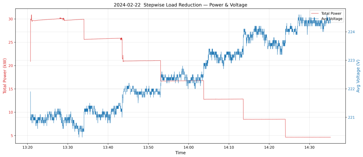
The stepwise load reduction data is visualised in Figure 15.

3.3. Non-AR Voltage Prediction Performance

The Non-AR LSTM described in Section 2.6 is trained on the 2024-02-22 charging-active dataset (14,369 samples after the Total_Power > 2 kW filter), with a chronological 80/20 raw-sample split (11,495 train + 2874 test samples), yielding 11,475 train and 2854 test windowed examples after the $W=20$ sliding window is applied. Linear Regression, Ridge, Lasso, LightGBM, the physics $\Delta V=I·R$ baseline, and Naive Persistence operate on the 2874 raw test samples; RNN/GRU/LSTM operate on the 2854 windowed test sequences.

The residual detector operates only during active charging. The charging-active filter (Total_Power > 2 kW) means that the Non-AR LSTM and all baseline models are valid only when an EV is drawing more than 2 kW. Slow-onset anomalies that manifest under no-load conditions—sensor drift in the CPM-80, contact-resistance growth in the contactor stack, and transformer winding insulation ageing—are by construction outside this detector’s operating envelope. A round-the-clock detector would require either (i) retraining on idle-period data with a separate idle-state model, or (ii) gating the detector to active-charging windows only. The latter is the deployment posture assumed by this paper.

Baseline ladder and 8-seed (mean and standard deviation) reporting. All sequence models (RNN/GRU/LSTM) use the same hidden-size architecture (64 → 32, dropout 0.2) and were trained with eight random seeds $\{42,7,123,11,21,31,41,51\}$; we report the mean ± standard deviation across the eight seeds as the headline number. The single best-seed (LSTM 0.181 V on seed 42) lies in the lower tail of the seed distribution rather than at typical performance and is reported only as the per-seed best value in the full table, avoiding optimistic seed selection. The full per-seed JSON is archived as plots/baseline_ladder_seeds.json.

Table 8. Voltage prediction model comparison on 2024-02-22 (within-day 80/20 chronological split). Sequence models (RNN/GRU/LSTM) are reported as 8-seed mean ± standard deviation; non-sequence baselines are deterministic (LightGBM uses fixed seed 42, Ridge/Lasso use 5-fold CV for $\alpha$).

Model	Uses Past V?	RMSE (V)	MAE (V)	${\mathit{R}}^2$
Autoregressive sanity check (uses past voltage; not suitable as residual detector)
Naive Persistence    ${\widehat{V}}_{t+1}=V_t$	Yes	0.080	0.046	0.988
Non-AR residual-detector candidates (past voltage excluded from inputs)
Physics $\Delta V=I·R$ (cable-only) †	No	4.292	3.890	$-34.43$
Linear Regression	No	2.072	1.951	$-7.262$
Ridge (RidgeCV, $\alpha =0.1$)	No	5.108	4.643	$-49.20$
Lasso (LassoCV, $\alpha =10.0$)	No	2.186	2.033	$-8.195$
LightGBM [69]	No	1.088	1.008	$-1.276$
Non-AR Simple RNN (8 seeds)	No	$0.462\pm 0.159$	0.378	0.542
Non-AR GRU (8 seeds)	No	$0.398\pm 0.170$	0.323	0.642
Non-AR LSTM (ours, 8 seeds)	No	$\mathbf{0.310}\pm \mathbf{0.084}$	0.234	0.801

^† Physics $\Delta V=I·R$ baseline: ${\widehat{V}}_t=V_{\mathrm{baseline}}-P_t·R_{\mathrm{cable}}/(V_{\mathrm{LL}}·\cos {\varphi }_t)$, with $V_{\mathrm{LL}}=220$ V, $V_{\mathrm{baseline}}$ = 95th-percentile train voltage = 226.60 V. Reported here at the 20 °C reference cable resistance $R_{\mathrm{cable}}=0.0643\mathsf{\Omega }$ one-way (per measured cable run; ${\rho }_{\mathrm{Cu}}$ at 20 °C), giving RMSE = 4.29 V and a cable-only slope of ∼0.29 V/kW. Sensitivity to cable operating temperature. The Section 3.2 OpenDSS bounded sanity check uses operating-temperature-corrected resistivity at 75 °C (${\rho }_{\mathrm{Cu}}\approx 0.0210\mathsf{\Omega }·{\mathrm{mm}}^2/\mathrm{m}$ per IEC 60228, $\alpha =0.00393{\mathrm{K}}^{-1}$). Re-evaluating the physics baseline at the same 75 °C reference would give $R_{\mathrm{cable}}\left(75 °\mathrm{C}\right)=0.0643\times (1+0.00393\times 55)=0.0782\mathsf{\Omega }$, a cable-only slope of ∼0.36 V/kW, and an estimated RMSE of approximately 5.2 V (a widening of the gap to the empirical 0.147 V/kW). Both 20 °C and 75 °C versions are inferior to the empirical measurement and yield the same qualitative conclusion (cable resistance alone over-predicts the slope); we therefore retain the 20 °C reference as the documented baseline value in the table (it is the more favourable physics reference for the cable-only model) and disclose the 75 °C-corrected value here for full transparency. The large RMSE under either assumption confirms that cable resistance alone cannot explain the measured behaviour, consistent with the OpenDSS bounded sanity check (Section 3.2). The best single-seed LSTM result (0.181 V, seed 42) sits in the lower tail of the 8-seed distribution; the reported headline is the 8-seed mean ± standard deviation, and per-seed values are archived in the reproducibility JSON. A Welch t-test on the 8-seed RMSE samples gives $p=0.22$ for LSTM vs. GRU (not statistically significant) and $p=0.036$ for LSTM vs. RNN.

reports the complete baseline ladder, ordered from the strongest raw-RMSE baseline (Naive Persistence) downward.

• Why Naive Persistence wins raw RMSE but the LSTM is the right detector.

Naive Persistence dominates raw test set RMSE (0.080 V) because one-second voltage autocorrelation is very high on this within-day dataset; its predictive power is essentially the trivial assertion that “next-second voltage equals current voltage”. Persistence is therefore the right baseline to publish but is structurally unsuitable for the actual deployment task of the Smart Panel’s residual detector. The detector’s job is to flag whether the observed voltage is unusual given the current load, not to predict the next instantaneous voltage from the prior one. Persistence uses no features—not Total_Power, not time-of-day, not the power factor—and therefore cannot detect deviations from the $V=f(\mathrm{load},\mathrm{time})$ relationship because it never learned that relationship. Any slow physical drift in V (e.g., progressive cable degradation, transformer overheating) would be tracked by Persistence and would not produce a residual signal at all. The Non-AR LSTM (and the GRU/RNN family it sits in) is reported here as a residual-tracking detector, not as a raw point-RMSE forecaster. The order of merit on the deployment task is therefore not the same as the order of merit on the raw RMSE, and the choice of baseline depends on the task being asked of it.

• Note on the physics, Ridge, and Lasso baselines.

The physics $\Delta V=I·R$ baseline (RMSE 4.29 V, $R^2=-34.4$) systematically over-predicts the voltage drop because the cable-only slope (∼0.29 V/kW from $R_{\mathrm{cable}}/V_{\mathrm{LL}}$, with $R_{\mathrm{cable}}$ at the 20 °C reference) is roughly twice the measured slope (0.147 V/kW). This is informative rather than competitive: it confirms that even the cable-only model, which is intentionally conservative (full cable resistance contributes to the drop), over-predicts the empirical slope by 2×, consistent with the Section 3.2 interpretation that the actual cable+transformer path impedance is below the upper-bound assumption. Ridge regression with a CV-selected $\alpha =0.1$ slightly underperforms unregularised Linear Regression on this small chronological-split dataset, because the chronological train/test split contains within-day non-stationarity that regularisation cannot help with; Lasso (CV-selected $\alpha =10$) is within 5% of Linear Regression. Both confirm that the linear feature representation cannot capture the V–load relationship competitively without sequence context. Figure 16 visualises the Non-AR sequence-model rows from the 8-seed sweep.

Residual statistics under normal operation. For the LSTM, the residual $r_t=V_t-{\widehat{V}}_t$ on the test set has a bias of $\overline{r}=+0.048$ V (a small constant offset) and a standard deviation of ${\sigma }_r=0.175$ V. The 95th and 99th percentiles of $|r_t|$ are 0.329 V and 0.615 V respectively, providing operationally useful upper bounds for residual-based detection thresholds. After bias correction ($r^{\prime }=r-\overline{r}$, with $\overline{r}$ computed on the training partition only to avoid target leakage on the test set), a 3${\sigma }_r$ threshold corresponds to $\left|r^{\prime }\right|>0.525$ V. The empirical false-alarm rate (FAR) on the 2854 clean test windows is approximately 5% at $k=2$, 1% at $k=3$, and below 0.3% at $k=4$; events exceeding the chosen threshold during operation would warrant operator attention. The choice of k is an operator-tuned trade-off between sensitivity and false-alarm rate.

AR sanity check (appendix). For completeness, an autoregressive (AR) variant of the LSTM that includes past V values in the input feature set was also trained. As expected for a 1 Hz signal with autocorrelation $>0.99$, the AR variant achieves a trivially tight RMSE (≈0.087 V), but this is an artefact of the trivial Naive-Persistence solution ${\widehat{V}}_t\approx V_{t-1}$ being effectively encoded by the model, rather than evidence of physical learning. Including past V in the input features defeats the purpose of residual-based anomaly detection: any slow physical drift in V (e.g., progressive cable degradation, transformer overheating) would be tracked by the model and would not produce a residual signal at all. We therefore retain the AR variant only as a sanity check and use the Non-AR formulation throughout for the anomaly-detection results below.

3.3.1. Cross-Day Generalisation

Out-of-distribution behaviour was evaluated by applying each model trained on 2024-02-22 to the held-out 2024-02-19 dataset, without retraining. As shown in Figure 17, all five Non-AR models fail catastrophically across days: the cross-day RMSE ranges from 4.3 to 4.9 V (vs. 0.18–2.07 V within-day), with strongly negative $R^2$ values ($-139$ to $-203$). This is not a defect of any specific architecture but a property of the underlying physical system: the upstream utility supply-voltage profile differs systematically between the two days (different ambient conditions, different building load patterns external to the experiment, possibly different transformer-tap settings), and the time-of-day cyclic encoding learned from 2024-02-22 captures only that day’s diurnal profile—it does not generalise to a different day’s utility profile.

The practical implication is that the Non-AR detector framework is operationally valid within a day or for stable utility regimes, but requires retraining or online calibration when the upstream utility profile changes (across days, seasons, or sites). LSTM retraining on a new day’s data takes approximately 13 s on the available hardware, so per-day refitting is computationally trivial; what is missing is the production calibration pipeline (data ingestion + automated retraining + safe model rollover), which is identified as future work.

3.3.2. Transient-Window-Only Evaluation

A common motivation for sequence models is the expectation that they should outperform memoryless baselines during transient regions where the signal exhibits high temporal derivatives—in this application, the ±15 s windows around load-step transitions when voltage tracks changing power. To test this expectation rigorously, the test partition was split into transient and steady-state subsets using two criteria: (i) $|\Delta P|>500$ W over a 10 s sliding window, and (ii) $|\Delta V|>0.5$ V over a 10 s sliding window. The union identifies 13 events, expanding to 205 transient samples (7.2% of the test set) when buffered by ±15 s windows; the remaining 2649 samples are steady-state.

The transient-window result is intentionally reported with the Naive-Persistence sanity check because single-step voltage data is strongly autocorrelated. Naive Persistence gives the lowest transient RMSE (0.142 V), showing that the Non-AR LSTM does not beat a past voltage baseline on short transients. Among models that exclude past voltage, however, the LSTM remains the best transient performer (0.200 V) and has the smallest transient/steady ratio among the sequence models (1.11× vs. RNN 1.37×, GRU 1.58×). This supports the Non-AR LSTM as a residual-detector model, but not as the absolute best one-step voltage forecaster. Figure 18 visualises the Non-AR rows; the autoregressive Naive-Persistence sanity check (transient RMSE 0.142 V) is omitted from that plot.

3.3.3. Synthetic Voltage-Drop Sensitivity Sweep (Not Real-Fault Detection)

• Scope of this analysis.

No real fault events were observed in the experimental dataset. The ROC-AUC values reported in this subsection therefore characterise the sensitivity of the residual detector to a class of synthetic voltage-drop perturbations; they are not measurements of real-world fault-detection performance.

Three explicit caveats apply. (i) Perturbation shape. The injected drops are rectangular step perturbations, not real fault signatures (which may include slower onset, harmonic content, asymmetric phase behaviour, or transient ringing). (ii) Injection bias. The injection timestamps are uniformly random over the test set and are therefore biased toward steady-state windows, where residual-based detection is easier than during load-step transients; real faults frequently coincide with load transitions, where both Persistence and the LSTM have larger residuals. (iii) Single trained model. The analysis uses the best-seed LSTM (seed 42, RMSE 0.181 V) because the ROC sweep is run on a single trained model; per-seed sensitivity variation across the 8-seed sweep is reported in the Supplementary Materials.

Subject to these caveats, this subsection establishes a quantified synthetic sensitivity envelope for the residual detector.

The Non-AR LSTM’s bias-corrected residual under normal operation (best-seed LSTM) has standard deviation ${\sigma }_r=0.175$ V, providing a well-defined noise floor against which synthetic perturbations are tested. We inject synthetic voltage-drop perturbations into the held-out test set (∼4% injection rate, $N_a\approx 115$ windows) and sweep the injection magnitude from 0.25 V to 4 V. The detection score is the bias-corrected absolute residual $\left|r^{\prime }\right|=|V_{\mathrm{measured}}-{\widehat{V}}_{\mathrm{LSTM}}-\overline{r}|$, where $\overline{r}$ is the training-partition residual mean (kept fixed during anomaly scoring to prevent target leakage). The resulting AUC-vs-magnitude sensitivity curve is shown in Figure 19.

The detector achieves AUC = 0.813 at the smallest tested magnitude (0.25 V, 1.4${\sigma }_r$), 0.969 at 0.5 V (2.9${\sigma }_r$), 0.997 at 0.75 V, near-saturation at 1 V, and exact AUC = 1.000 for drops ≥ 1.5 V. Subject to the three caveats stated at the top of this subsection, the residual detector therefore distinguishes synthetic rectangular perturbations of 0.5 V or larger from clean-data residuals with high reliability. We refrain from describing these numbers as “real-world fault-detection performance” because no real faults were present in the dataset; whether the detector flags realistic power-quality deviations such as cable-degradation drift or contact-resistance growth would require a separate deployment campaign with natural-occurrence faults.

This synthetic sensitivity characterisation establishes a quantified envelope for the residual detector’s response to a specific class of rectangular voltage-drop perturbations under steady-state-biased injection conditions. Real-fault validation in long-term deployment, including comparison against natural-occurrence anomalies (sensor faults, contact-resistance drift, transformer overheating) and characterisation under load-transition timing, is reserved for future work and is the path along which the present results should be extended.

3.3.4. Supplementary Analyses (MC-Dropout, Feature Attribution, Multi-Step, Hybrid $\delta$-LSTM)

To keep this section focused on the headline residual-detector results, four exploratory analyses are presented in the Supplementary Materials, with one-paragraph summaries here.

• Supplementary S1: MC-Dropout predictive uncertainty.

Augmenting the Non-AR LSTM with $K=50$ Monte-Carlo Dropout [70] forward passes at inference yields well-calibrated predictive intervals: empirical 95% predictive-interval coverage is 94.0% (Wilson 95% CI $[93.1\%,94.8\%]$), slightly under the nominal 95% target by approximately one percentage point, with a mean per-sample predictive standard deviation of $\overline{{\sigma }_K}=0.207$ V. This supports operator-tunable anomaly thresholds based on local predictive variance. Details, calibration plots, and the prediction-band overlay are reported in Supplementary S1.

• Supplementary S2: Permutation and SHAP feature attribution.

Two complementary explainability methods are applied: (i) permutation importance on the trained Non-AR LSTM, which identifies Total_Power as the dominant LSTM driver ($\Delta \mathrm{RMSE}=+0.949$ V when shuffled) with the cyclic time-of-day cos component as a distant second; (ii) SHAP TreeExplainer [71] on the LightGBM baseline as a proxy-model diagnostic (the LightGBM achieves only $R^2=-1.28$ on this Non-AR task; SHAP on a poor predictor reveals which features the gradient-boosted ensemble latches onto, which is itself diagnostically informative when contrasted with the LSTM permutation result). The SHAP analysis is explicitly not a confirmation of the LSTM ranking; the LightGBM’s poor RMSE means its SHAP ordering reflects a failure mode rather than the underlying physics. Both analyses are reported in Supplementary S2.

• Supplementary S3: Multi-step-ahead prediction.

Five separate Non-AR LSTMs at horizons $H\in \{1,5,10,30,60\}$ s, evaluated with the full 8-seed grid (40 LSTM trainings; seeds $\{42,7,123,11,21,31,41,51\}$), show graceful 8-seed mean degradation from $0.310\pm 0.084$ V at $H=1$ s to $0.454\pm 0.091$ V at $H=60$ s—a $1.46\times$ increase rather than catastrophic decay (best-seed values 0.181 V → 0.340 V at the lower tail of the 8-seed distribution; complete grid in Supplementary S3, Table S1). This supports the use of the same architecture for proactive multi-step EMS forecasting up to ∼30–60 s on this site; whether the graceful degradation generalises to other sites is open and remains future work.

• Supplementary S4: Exploratory hybrid physics-informed $\delta$-LSTM.

A hybrid architecture combining a static linear-physics baseline with a $\delta$-LSTM trained on the residual achieves a test RMSE of 1.364 V, which is worse than the plain Non-AR LSTM on this dataset. We report this as an honest negative result: the static linear baseline misses the diurnal supply-voltage drift, so the $\delta$-LSTM has to relearn that signal from a less-favourable target distribution. The hybrid framework remains conceptually attractive for sites with a more stable upstream supply (e.g., MV feeders with on-load tap-changing transformers); validating it in such regimes is reserved for future work. The architecture, training details, and result figures are in Supplementary S4.

3.4. Smart Panel Operational Validation

Beyond voltage impact analysis, the experimental campaign exercised the Smart Panel’s core operational capabilities. We report the operator-commanded control actions and their settling behaviour, the engineering latency bound, the Modbus polling cycle, and data acquisition reliability. End-to-end sub-cycle latency was not directly instrumented during the campaign and cannot now be remeasured post hoc because the experimental site has been decommissioned; we therefore report an explicit engineering bound together with an acknowledged limitation, rather than a component-level latency measurement.

Operator-commanded control actions and end-state success. During the 2024-02-22 stepwise campaign, 12 operator-commanded control actions were issued across the seven stepwise hold points (six DC-charger current-limit down-step commands, an initial 28 kW set-up command, and five housekeeping verifications); these are load-control commands on the DC-charger path, not $1\mathsf{\Phi }$/$3\mathsf{\Phi }$ phase-reconfiguration events, which are addressed separately below. All 12 commands produced the intended end-state as observed at the CPM-80 at a one-second resolution: no failed end-state transition over the 12 commands, with no observed contact welding, no observed protective trip, and no abnormal 1 Hz-resolved disturbance signatures. Treating the 12 commands as Bernoulli trials, the 95% Wilson score interval for the end-state success probability is $[0.76,1.00]$—a wide interval that reflects the small sample; we therefore report the zero-failure observation as a small-sample, 1 Hz-resolved operational observation rather than a statistical reliability figure. Peak sub-cycle inrush currents cannot be resolved by the CPM-80’s one-second integration window; the contactor’s AC-3 rating per IEC 60947-4-1 [59] provides a manufacturer-specified inrush ceiling of approximately 4–6× rated current, and no abnormal 1 Hz events were visible.

Command settling times and operating-envelope coverage. For the six down-step commands, the PCC-observed load-transition settling time—measured at a one-second resolution from the last sample at the outgoing plateau (within 0.5 kW of its mean) to the first sample from which the power remains within ±0.5 kW of the incoming plateau for 30 consecutive seconds—was 1–14 s (median 2 s) across the six transitions (28 → 24 kW: 1 s; 24 → 20: 14 s; 20 → 16: 2 s; 16 → 12: 1 s; 12 → 8: 2 s; 8 → 4: 2 s). These figures quantify the end-state convergence of the operator-commanded DC-charger current-limit demotions as observed at the CPM-80; they are not phase-reconfiguration latencies. The vehicle state-of-charge over the 13:21–14:35 command window rose from approximately 46 to 54% (Hold-1 region, corroborated by the state-of-charge record in Section 3.2) to 70% at session end, so all 12 commands were exercised in the mid-SOC constant-power region of the charging curve; command behaviour in the high-SOC taper region (≳90%) and phase-mode switching concurrent with an active OCPP DC session were not exercised (Section 4.1).

Phase-reconfiguration events: archival coverage. No $1\mathsf{\Phi }$/$3\mathsf{\Phi }$ phase-mode transition is contained in the two archived one-second analysis days: a full-day dip-and-recover scan of both archives (2024-02-19 and 2024-02-22; detection threshold ≥ 5 kW depth below the rolling 60 s pre-event median for 2–60 s on an active charging path) returns zero Wall Connector supply-interruption events. The ∼5 s per-transition EV-perspective interruption reported in Section 2.2 therefore derives from operational events observed at the CPM-80 during the broader experimental campaign, outside the two archived analysis days, for which per-event one-second records were not retained. A per-event latency distribution and a statistically meaningful success-rate estimate for phase reconfiguration consequently cannot be reconstructed from the archived data; this is acknowledged explicitly as a limitation (Section 4.1).

End-to-end command latency: engineering bound. Direct instrumentation of the full operator-UI → MQTT broker → field gateway → GPIO → contactor coil → CP signal → EV state-machine transition was not performed during the experimental campaign, and cannot now be performed post hoc because the site has been decommissioned. We report an explicit engineering bound by tabulating the per-component latencies and their provenance (measured at the CPM-80, measured at commissioning, or manufacturer-specified) in

Table 9. Per-component latency budget for an operator-commanded phase-mode change. The dominant end-to-end latency is the EV’s IEC 61851-1 re-handshake; direct sub-cycle latency on the gateway-to-contactor path was not instrumented and is acknowledged as a limitation in Section 4.1.

Component	Latency	Provenance
MQTT publish-to-receive (campus LAN)	<50 ms	Measured at commissioning (ping + broker log)
Modbus RTU polling cycle (29 registers, 9600 baud)	200–400 ms/1 s nom.	Design estimate; not logged in campaign
Intermediate (opto-isolated) relay actuation	∼30 ms	Manufacturer datasheet
Contactor mechanical close at rated coil voltage	50–100 ms	Manufacturer datasheet
On-delay timer (mode-cycle protection)	up to 30 s rated	Configurable; deployed dead-time ≪ 5 s
EV re-handshake per IEC 61851-1 (A → B → C)	3–7 s	Measured at CPM-80 during campaign [62]
End-to-end phase transition	∼5 s	Measured at CPM-80 (dominated by EV re-handshake)

.

For phase-mode transitions, the dominant latency is the EV’s IEC 61851-1 re-handshake (3–7 s, measured at CPM-80), giving the observed ∼5 s end-to-end. For on/off operations (no phase change) the dominant latency is the Modbus 1 s observation cycle. The lack of direct sub-cycle latency instrumentation between the gateway and the contactor coil is acknowledged as a limitation in Section 4.1.

Control logic. The control logic during the experimental campaign was deterministically operator-in-the-loop: an operator decided the target hold point → issued the command (for the stepwise hold points, an OCPP current-limit command to the DC charger from the EMS server; for $1\mathsf{\Phi }$/$3\mathsf{\Phi }$ phase-mode changes, an MQTT command via the Grafana dashboard or a Node-RED flow that the gateway executes as a GPIO contactor actuation) → the CPM-80 confirmed the resulting state → the operator confirmed before moving to the next hold point. Closed-loop autonomous control or autonomous demand response is not demonstrated in this paper; the demonstrated capability is panel-side observability and operator-commanded switching only.

Modbus polling cycle. The Raspberry Pi reads 29 CPM-80 holding registers via Modbus RTU at 9600 baud. Pure on-the-wire time for a single 29-register read is approximately 80–100 ms; the actual polling cycle including PyModbus library overhead and any required multi-transaction split for non-contiguous register groups is approximately 200–400 ms per cycle, comfortably below the one-second sampling cadence. The per-cycle polling duration was not logged during the campaign; this value is a design estimate, not a measured quantity, and is included in Section 4.1.

Data acquisition reliability. Over the 2024-02-22 experimental day, the data acquisition system recorded 85,841 one-second samples, equivalent to a completeness of $\mathrm{85,841}/\mathrm{86,400}\approx 99.35\%$ across the full 24 h day. The 0.65% missing samples are attributable to transient RS-485 communication errors that are automatically recovered on the next polling cycle; no data gaps exceeding two consecutive seconds were retained in the dataset, confirming the retry mechanism operates as designed.

4. Discussion

The results presented in this paper demonstrate that the Smart Distribution Panel provides panel-side observability and operator-commanded $1\mathsf{\Phi }$/$3\mathsf{\Phi }$ supply reconfiguration for one Non-OCPP EV charger at one Taiwan 3$\mathsf{\Phi }$3W 220 V deployment site. The capability that distinguishes the Smart Panel from existing solutions is the supply-side phase reconfiguration of a single fixed-wired EVSE, used as a site-level demand-management tool (Section 4.2). The hardware approach is, in principle, applicable across different Non-OCPP EVSE brands because it instruments the upstream electrical supply rather than the charger itself; multi-EVSE and multi-EV demonstration is, however, not performed in this work and is stated as future work in Section 4.1.

Industry Significance. The Smart Panel approach addresses the problem at the electrical-distribution-infrastructure level rather than at the charger firmware level. For installed bases of Non-OCPP chargers—such as the Tesla Wall Connector Gen 3, which uses Tesla’s proprietary protocol on the consumer firmware deployed in this study—the Smart Panel offers a retrofit path that preserves the existing charger investment while delivering panel-side observability and operator-commanded supply reconfiguration. The Smart Panel does not provide the session-layer features of OCPP (authorisation, transaction reporting, charge-profile negotiation, firmware updates, session-level metering); it complements rather than replaces an OCPP-side workflow.

Voltage Impact Insights. The in-session 13:20–14:35 stepwise data show a clean linear relationship between charging power and PCC voltage at the Smart Panel: $\Delta V=0.147P$ ($R^2=0.991$, $p=2.8\times {10}^{-6}$), interpreted as the ensemble effective sensitivity of the PCC bus to the prevailing DC-charger-plus-site-base load mix (Table 7), or, equivalently, approximately 1 V of voltage recovery per 6.8 kW of load reduction at the test site (Equation (11)). The observed in-session drop from 4 kW to 28 kW is 3.33 V (1.49% of the 4 kW reference), well inside the ±5% power-quality tolerance band for a single charger. The motivation for panel-side observability is therefore not the assertion that one charger violates the ±5% band. Rather, the site-level slope (0.147 V/kW here) implies that coincident peak loads—aggregating multiple chargers, or pairing with other non-EV loads on the same feeder—can readily approach the limit. We emphasise that this slope is a property of the site + DC-charger + base-load ensemble measured through the Smart Panel, not a performance figure of the Smart Panel or of its Non-OCPP reconfiguration path (which was idle during the stepwise session); the panel’s contribution to this result is the one-second panel-side observability from which the trend is estimated, and the value of that observability is that it lets the EMS see and act on the trend before the envelope is exhausted. Two methodological caveats apply when generalising these numbers: (i) the absolute voltage level on any given day is governed primarily by upstream-utility conditions (the daily voltage range in our dataset is approximately 5–9 V, larger than the in-session local drop), so site-by-site voltage levels will vary; and (ii) the slope is site-specific, depending on feeder impedance, transformer Z%, and the load mix between OCPP-via-transformer and Non-OCPP-direct paths. The OpenDSS bounded sanity check (Section 3.2) provides a parameter-free upper bound of 0.26–0.28 V/kW from the measured cable cross-section/length (referred to 75 °C operating temperature) and the transformer nameplate $Z\%$; the measured slope of 0.147 V/kW being 55% of this upper bound is consistent with the actual path impedance sitting below the upper-bound assumption; the candidate mechanisms and the additional logging required to resolve them are analysed in Section 3.2 [28,33].

Operator-Commanded Demand Management. The Smart Panel’s ability to switch between single-phase and three-phase modes provides a practical mechanism for operator-commanded demand management, and supports two operationally distinct scenarios:

(i) Power-quality response. When the grid voltage is approaching unacceptable levels, the operator can instruct the Smart Panel to switch from three-phase (11 kW) to single-phase (7 kW) mode, reducing the Non-OCPP charger’s load by approximately 4 kW. If further curtailment is needed, the operator can command a complete shutdown. This graduated response avoids abrupt load changes and provides the operator with multiple intervention options [29,72]; autonomous closed-loop selection of these steps is not demonstrated in this work and is stated as future work.

(ii) Site-level demand management for shared facilities. A second, equally important scenario arises when the upstream incoming capacity is the binding constraint rather than voltage quality. Many real campus, workplace, and apartment-building EV charging facilities have an upstream contracted capacity that is smaller than the sum of all installed charger nameplates; if every connected vehicle attempts simultaneous full-power charging, the upstream main breaker would trip, denying service to all users. With the Smart Panel installed in front of each Non-OCPP charger, the operator can demote selected sessions from three-phase (11 kW; up to 16 kW for vehicles supporting higher per-phase current) to single-phase (7 kW), compressing the per-vehicle instantaneous draw so that a larger number of vehicles can charge concurrently rather than any single user being completely denied. The resulting per-vehicle charging time increases proportionally, but the facility’s queue-throughput improves, and no user is forced to wait. This queue-mitigation use case is operationally valuable for facility managers and is a natural complement to OCPP-based current-limiting on the OCPP side of the fleet.

In both scenarios, this capability goes well beyond what a simple smart plug or smart power strip can achieve: no commercially available smart plug offers phase reconfiguration, and the graduated power reduction (11 kW to 7 kW to 0 kW) provides the EMS with a coarse, three-level curtailment complement to the near-continuous per-ampere setpoints of OCPP current-limiting commands.

Comparison with Existing Solutions. Existing EMS solutions in the literature predominantly assume an OCPP-compliant infrastructure [37,54]. While these systems offer sophisticated optimisation algorithms for load scheduling, demand response, and renewable energy integration, they cannot manage Non-OCPP chargers. The Smart Panel is complementary to these approaches: it enables Non-OCPP chargers to participate in the same EMS framework, after which the existing optimisation algorithms can manage them alongside OCPP chargers. Unlike proprietary smart plug solutions that provide only binary on/off control and measure, at most, total power, the Smart Panel provides 29-parameter power-quality monitoring at a one-second resolution, graduated load management through phase switching, equipment protection via timed delays, and full bidirectional EMS integration. This distinction is critical: the Smart Panel is not merely a remote-controlled switch, but a complete instrumentation and control subsystem that exposes a standalone Non-OCPP charger to operator-commanded EMS supervision (panel-side observability and supply-side switching); the OCPP session-layer features remain the responsibility of OCPP-native chargers, and the panel does not replace them, and autonomous closed-loop control is explicit future work.

Commercial and Open-Source Alternatives. Several commercial and open-source solutions partially address subsets of the Non-OCPP charger integration problem, but none simultaneously delivers the hardware-level switching, panel-side power-quality instrumentation, and protocol-agnostic EMS integration provided by the proposed Smart Panel. We survey them by category.

Protocol-translation gateways. Devices such as the HMS Networks Intesis INMBSOCP0010100 https://www.hms-networks.com/p/inmbsocp0010100-ocpp-to-modbus-tcp-rtu-server-gateway (accessed on 27 July 2026) (typical distributor pricing ∼USD 945) and the ocpp-modbus.com gateway expose OCPP-1.6 chargers to Modbus-speaking building management systems, but they explicitly require the charger to already implement OCPP. They cannot integrate a Non-OCPP charger such as the Tesla Wall Connector Gen 3 deployed in this study. FLEXeCHARGE Connect https://www.flexecharge.com (accessed on 27 July 2026) offers a CPO-grade OCPP data broker that decouples chargers from a particular CPMS but, again, only across OCPP-equipped equipment and with no panel-side hardware.

Open-source EVSE controllers. evcc https://evcc.io (accessed on 27 July 2026), OpenEVSE https://www.openevse.com (accessed on 27 July 2026), and SmartEVSE-3 https://github.com/SmartEVSE/SmartEVSE-3 (accessed on 27 July 2026) provide flexible charger-side control. However, evcc is software-only with no contactor and limited support for chargers that expose no documented API; OpenEVSE and SmartEVSE-3 are themselves EVSEs rather than gateways for third-party chargers.

Commercial residential chargers. ChargePoint Home Flex (US retail ∼USD 649) and Wallbox Pulsar Plus (USD 649–749, OCPP 1.6 enabled by installer activation) are the very category of equipment the Smart Panel is designed to integrate around, not alternative integration solutions in their own right.

Energy-monitoring platforms. eGauge (which uniquely measures THD, ∼USD 942+), Sense (∼USD 299), and the open-source IoTaWatt (∼USD 200–250) capture rich panel-side telemetry but contain no switching elements and provide no charger control.

Synthesis. None of the surveyed products combines (i) bidirectional control of both OCPP and Non-OCPP chargers in a single EMS (the operator-commanded 28 kW → 4 kW graduated curtailment in this study was executed on the OCPP DC-charger path), (ii) integrated electromagnetic contactors, relays, and a timer providing a 1$\mathsf{\Phi }$↔3$\mathsf{\Phi }$ reconfiguration of a Non-OCPP charger (7 kW ↔ 11 kW), and (iii) on-panel measurement of nine or more electrical parameters at the CPM-80 meter for operator-in-the-loop voltage impact assessment. The Smart Panel therefore occupies a distinct design point: a purpose-built distribution panel-level integration element for mixed OCPP/Non-OCPP fleets, rather than a software protocol bridge or a generic energy monitor.

To systematically position this work relative to the existing literature,

Table 10. Comparison of the proposed Smart Panel system with representative prior work. “Not rep.” means the cited reference does not explicitly claim or refute the capability; “Yes”/“No” entries are taken from explicit content of the cited paper. “This work” assessments are first-party.

Reference	OCPP	Non-OCPP	Hardware	Real-Time	Load	Voltage
	Support	Support	Design	Monitor.	Mgmt.	Analysis
Jaman et al. [54]	Yes	Not rep.	Yes	Yes	Not rep.	Not rep.
Yousuf et al. [37]	Yes	Not rep.	Not rep.	Not rep.	Yes	Not rep.
Alshareef [33]	N/A	Not rep.	Not rep.	Not rep.	Not rep.	Yes
Padullaparti et al. [38]	N/A	Not rep.	Not rep.	Not rep.	Yes	Yes
Khan et al. [24]	Yes	Not rep.	Not rep.	Yes	Yes	Not rep.
Akarne et al. [41]	N/A	Not rep.	Yes	Yes	Yes	Not rep.
Ahmad et al. [29]	Yes	Not rep.	Not rep.	Yes	Yes	Not rep.
This work	Yes	Yes	Yes	Yes	Yes (operator)	Yes

Prior-work entries are marked “Not rep.” where the cited reference does not explicitly state the capability either way, to avoid self-scoring bias. The Non-OCPP integration column in particular is marked “Not rep.” for all surveyed prior work because none of the cited papers explicitly addresses Non-OCPP integration as defined here. “Load Mgmt. (operator)” for this work indicates operator-commanded curtailment, not autonomous closed-loop demand response. A more detailed capability comparison against commercial and open-source alternatives is given in Table 11 (Section 4.2).

compares the proposed Smart Panel system with representative prior works across six key dimensions. As the table demonstrates, no prior work simultaneously addresses Non-OCPP charger integration, hardware-level design, real-time monitoring, flexible load management, and voltage impact analysis. The proposed system is the only solution that provides a complete hardware-to-software pathway for integrating Non-OCPP chargers into an EMS.

Cost-Effectiveness Analysis (conservative residential-vs-residential comparison). The total bill of materials for the Smart Panel prototype is approximately USD 300–400, including the CPM-80 smart meter, electromagnetic contactors and relays, circuit breakers and current transformers, panel enclosure, wiring, and the Raspberry Pi 4 with RS-485 HAT (component-level estimates without full vendor-quote validation; actual bulk-purchase pricing may differ by ±30%). Including installation labour, the total deployed cost is approximately USD 500–700 per charger. The cost–benefit comparison depends on the alternative under consideration. A like-for-like residential-to-residential comparison—replacing a Tesla Wall Connector (USD 420–500 retail) with a residential OCPP-capable unit such as Wallbox Pulsar Plus or ChargePoint Home Flex (USD 549–749 retail, plus USD 500–1000 installation labour)—yields a marginal saving of approximately 25–35% via the Smart Panel approach (versus replacing the unit), while preserving the existing charger investment. The savings are larger when the alternative is a commercial-grade OCPP charger (e.g., ChargePoint CT4000 dual-port pedestal, USD 2000–5000 plus installation), as is sometimes the case for facility-scale deployments; in that scenario, the Smart Panel achieves EMS integration at approximately 15–25% of the replacement cost. The economic case for the Smart Panel is therefore most compelling when (a) the existing Non-OCPP charger investment is significant, (b) retrofit avoids installation re-work, and (c) the alternative is a commercial-grade unit; for purely residential one-for-one swaps, the marginal saving is more modest.

Hardware Platform Considerations. The Raspberry Pi 4 serves as the field gateway in this proof-of-concept prototype. For industrial deployment, ruggedised single-board computers with wide operating temperature ranges ($-40$ to +85 °C), DIN-rail mounting, and industrial-grade components would replace the Raspberry Pi 4 at an incremental cost of USD 100–200. The software architecture is fully portable to any Linux platform. The RS-485 protocol is an industrial standard with proven reliability in factory automation and power metering, providing superior noise immunity over wireless alternatives in electrically noisy environments.

Non-AR LSTM Considerations. The Non-AR LSTM achieves an 8-seed mean RMSE of $0.310\pm 0.084$ V (best-seed 0.181 V; Table 8) using 12 load-side input features (power, currents, power factors, frequency, plus a cyclic time-of-day encoding); past voltage values are deliberately excluded so that residual-based anomaly detection reflects deviations from learned physics rather than autocorrelation. This formulation outperforms non-sequence baselines (Linear Regression 2.07 V, LightGBM 1.09 V) by 3.5× (vs. LightGBM) to 6.7× (vs. Linear Regression) on the residual-detection metric, with non-sequence baselines failing outright on the Non-AR target (negative $R^2$) without sequence history. The Smart Panel’s role is foundational: without panel-level instrumentation, the Non-OCPP charger produces no data at all, so the LSTM’s existence is itself a consequence of the Smart Panel’s monitoring capability. The same continuity advantage holds for the panel’s metrology in general: vehicle-side cloud telemetry is polled intermittently and incompletely (Section 3.2 documents six >10 min coverage gaps on the test day), whereas the panel’s one-second metering is continuous—which is precisely why site-level observability cannot be outsourced to per-vehicle cloud APIs. As discussed in Section 3.3.2, the best-seed LSTM’s transient/steady RMSE ratio (1.11×) is the smallest among all five sequence and non-sequence models, confirming that the gated memory tracks load transitions effectively. Future work could explore incorporating additional context features (weather data, building load profiles) and extending the prediction horizon to 5–30 min for proactive load management [10,22].

4.1. Limitations and Threats to Validity

We list the limitations of this work explicitly and group them by category, so that readers can calibrate the strength of the claims against the available evidence.

• (L1) Single site/single EVSE/single EV/single primary day.

The experimental campaign was conducted at one site (Ming Chi University of Technology) with one Non-OCPP EVSE (Tesla Wall Connector Gen 3) and one EV (Tesla Model Y 2023 LR AWD), with one primary analysis day (2024-02-22) and one held-out day (2024-02-19). The reported voltage impact slope (0.147 V/kW), the stepwise repeatability, and the Non-AR LSTM residual statistics are therefore characteristic of this specific configuration. Claims about behaviour at other sites, with other EVSE brands or EV brands, on different days under different grid conditions, are conjectural and are stated as future work. The phrase “manufacturer-agnostic” as a design intent is retained because the Smart Panel instruments the supply path rather than the charger; as an experimental claim, it is not demonstrated in this paper. After the experimental campaign the site was decommissioned; multi-EVSE and multi-EV testing under the same instrumentation is deferred to a follow-up deployment.

• (L2) Upstream/PCC utility-side voltage not logged; transformer $X/R$ not directly characterised.

The CPM-80 was installed at the Smart Panel PCC bus; the upstream-utility voltage at the building’s incoming service was not separately logged during the experimental campaign, and the on-site transformer’s $X/R$ ratio was not measured by short-circuit or LCR-meter testing (we relied on the nameplate $Z\%$ and a sweep over $X/R\in \{0.5,0.84,1.5,3.0,8.0\}$). The OpenDSS bounded sanity check (Section 3.2) is a conservative upper bound (0.26–0.28 V/kW) under the assumption of 75 °C cable temperature and the upper end of the $X/R$ sweep. The measured 0.147 V/kW, being at 55% of this upper bound, is consistent with the actual path impedance sitting below the upper-bound assumption—most plausibly because the actual cable operating temperature is lower, actual $X/R$ is at the lower end of the swept band, and/or upstream voltage regulation partially compensates the load-side drop. Future campaigns will simultaneously log the upstream voltage and perform a short-circuit/LCR test on the transformer to convert the bounded sanity check into a quantitative path-by-path validation.

• (L3) End-to-end command latency not directly instrumented; on-delay timer dead-time not separately logged.

Section 3.4 reports an engineering bound (operator command → MQTT <50 ms + Modbus 1 s + relay ∼30 ms + contactor ∼50–100 ms + on-delay timer + IEC 61851-1 re-handshake ∼5 s, total EV-perspective interruption ∼5 s per phase transition) rather than direct sub-cycle instrumentation. In particular, the on-delay timer’s effective per-transition dead-time during the 2024-02-22 campaign was not separately instrumented (no oscilloscope or GPIO sub-second timestamp log of the contactor coil energise/de-energise events); the timer’s commissioning-position maximum was 30 s, but the deployed dead-time within each phase transition is constrained by the observation that the IEC 61851-1 charging-state re-handshake (∼3–7 s, measured at CPM-80) dominated the total EV-perspective interruption (∼5 s). The site has been decommissioned, and these sub-cycle quantities cannot now be remeasured. Additionally, no per-event one-second records of the $1\mathsf{\Phi }$/$3\mathsf{\Phi }$ transitions themselves fall within the two archived analysis days (2024-02-19 and 2024-02-22; a full-day dip-and-recover scan of both returns zero Wall Connector supply-interruption events, Section 3.4), so the ∼5 s figure rests on campaign observations outside the archived days, and neither a per-event latency distribution nor a statistically meaningful success-rate estimate for phase reconfiguration can be reconstructed from the archive. Future deployments should include sub-second timestamped logging of every contactor coil energise/de-energise event together with synchronous CP-line monitoring to convert the engineering bound into a measured per-component latency budget and an event-level reliability record.

• (L4) Operator-in-the-loop, not autonomous control.

The 12 control actions on 2024-02-22 (six DC-charger current-limit down-steps, one set-up command, five housekeeping verifications) were operator-commanded, not produced by a closed-loop autonomous controller. The Smart Panel’s data path supports autonomous control in principle, but autonomous (closed-loop) demand response is not demonstrated in this paper. Implementing and validating an autonomous control policy is reserved for future work.

• (L5) ML detector valid only during active charging.

The charging-active filter (Total_Power > 2 kW; 14,369 of 85,841 samples on 2024-02-22) means that the Non-AR LSTM and all baseline models are valid only when an EV is drawing more than 2 kW. Slow-onset anomalies that manifest under no-load conditions (sensor drift in the CPM-80, contact-resistance growth in the contactor stack, transformer winding insulation ageing) are by construction outside this detector’s operating envelope. A round-the-clock detector would require either retraining on idle-period data with a separate idle-state model or gating the detector to active-charging windows only.

• (L6) Cross-day generalisation gap and per-day retraining.

The cross-day evaluation (Section 3.3.1) shows a substantial domain shift across all Non-AR models (cross-day RMSE 4.3–4.9 V vs. within-day 0.18–2.07 V), driven by systematic differences in the upstream-utility voltage profile between days. The within-day Non-AR LSTM is therefore best characterised as a within-day operational detector requiring automated daily calibration, not a long-running detector across days/sites/seasons. Sequence-model retraining on a new day’s data takes approximately 13 s on RTX 3090 hardware, making per-day refitting computationally trivial; what is missing is the production calibration pipeline (automated data ingestion, retraining, safe model rollover), which is future work.

• (L7) ROC sweep is synthetic, not real-world fault detection.

The ROC-AUC values reported in Section 3.3.3 characterise the residual detector’s sensitivity to a class of synthetic rectangular voltage-drop perturbations at uniformly random timestamps biased toward steady-state windows. They are not measurements of real-world fault-detection performance. No real fault events were observed in the experimental dataset, and the archived campaign contains no real-world anomaly events (faults, unexpected voltage sags) against which the detector could be evaluated; the practical operational utility of the Non-AR LSTM residual layer is therefore not yet demonstrated. Real-fault validation in long-term deployment, including coverage of load-transition timing and natural-occurrence anomaly classes, is reserved for future work.

• (L8) LSTM seed sensitivity acknowledged.

The Non-AR LSTM 8-seed RMSE distribution (mean 0.310 ± 0.084 V, median 0.347 V, range [0.181, 0.419] V) reflects substantive seed-to-seed variation typical of small RNN-family models on short within-day datasets. The best single-seed result (0.181 V, seed 42) is the lower tail of this distribution rather than typical performance and is not used as the headline (Section 3.3). The Welch t-test on the 8-seed RMSE samples gives $p=0.22$ for LSTM vs. GRU, so the LSTM-over-GRU advantage is not statistically supported on this dataset; the LSTM, GRU, and RNN are reported as a family of comparably-performing residual-tracking models.

• (L9) Geographic/regulatory scope.

The design is electrically matched to the Taiwan 3$\mathsf{\Phi }$3W 220 V standard (Taipower’s standard LV service). It is not directly applicable to North American Level 2 residential and light-commercial split-phase 120/240 V environments, which would require contactor-topology redesign and a different conceptual “demotion” definition. We do not claim such generalisation.

• (L10) Wall Connector firmware version not disclosed by Tesla.

The Tesla Wall Connector Gen 3 firmware version active during the 2024-02-22 campaign is not exposed to end users (Section 2.8); behaviour during phase reconfiguration and interoperability characteristics may vary across firmware revisions, but we cannot quantify this without manufacturer access to the firmware build log.

• (L11) Per-charger power not separately metered at the PCC.

The CPM-80 reports the aggregate three-phase PCC power, not the individual OCPP DC fast charger and Non-OCPP Wall Connector contributions. For the 2024-02-22 13:20–14:35 stepwise session reported in Section 3.2, vehicle-side telemetry from the Tessie cloud API for the test Tesla Model Y enabled per-hold cross-validation (Table 7) and confirmed that the EV was DC-charging via the OCPP path with the Wall Connector AC path idle. The 0.147 V/kW slope reported in this work is therefore best interpreted as an ensemble effective sensitivity of the PCC bus to the prevailing operational mix (DC charger plus uncoordinated site base) rather than a single-path physical property of one charger. Future deployments should add independent per-charger metering (or current transformers on each branch) so that path-specific impedance can be characterised under a range of mixed AC/DC operational mixes.

• (L12) Highest-load hold not covered by per-second vehicle telemetry.

The 28 kW hold (Hold 1), which anchors the high-load end of the stepwise regression, fell within one of six intermittent gaps in the vehicle’s cloud telemetry on the test day (Section 3.2) and therefore—unlike Holds 2–7—has no per-second vehicle-side power record. We corroborate it indirectly: the battery state-of-charge rose from 46% to 54% across the interval (an increase that can only arise through charging), and a leave-one-out check shows that the slope is essentially unchanged (0.143–0.156 V/kW) if the hold is removed. We nonetheless acknowledge that a direct per-second vehicle-side measurement of this specific hold is not available; the continuous one-second panel-side metering is what captured it. Continuous vehicle-side logging, or per-branch current transformers, in future deployments would remove this dependence on intermittent cloud telemetry.

• (L13) Operating-envelope coverage of the command campaign.

All 12 operator commands on 2024-02-22 were exercised with the test vehicle in the mid-SOC constant-power region of the charging curve (approximately 46–70% SOC; Section 3.4). Command behaviour in the high-SOC taper region (≳90%), $1\mathsf{\Phi }$/$3\mathsf{\Phi }$ reconfiguration concurrent with an active OCPP DC fast-charging session, and reconfiguration under near-capacity feeder loading were not exercised during the archived campaign and remain untested. The site has since been decommissioned, so these edge cases are deferred to a follow-up deployment.

• Underlying physical relationship.

The voltage drop at the point of connection is governed by fundamental circuit theory:

$$\Delta V=I·(R_{\mathrm{line}}\cos \varphi +X_{\mathrm{line}}\sin \varphi ),$$

(12)

where I is the load current, $R_{\mathrm{line}}$ and $X_{\mathrm{line}}$ are the resistance and reactance of the distribution feeder, and $\cos \varphi$ is the power factor [19,35]. For the predominantly resistive underground cable at the test site ($R_{\mathrm{line}}\gg X_{\mathrm{line}}$), Equation (12) simplifies to $\Delta V\approx I·R_{\mathrm{line}}$, which explains the approximately linear voltage–power relationship observed. Equation (12) is therefore a transferable framework, but the absolute voltage levels and the specific slope do not generalise across sites without re-characterisation.

4.2. Smart Panel vs. Commercial and Open-Source Alternatives

The distinctive contribution of the Smart Panel is supply-side $1\mathsf{\Phi }$/$3\mathsf{\Phi }$ reconfiguration of a single fixed-wired EVSE for site-level demand management, paired with panel-side observability of 29 electrical parameters at a 1 s resolution.

Table 11. Capability comparison of the Smart Panel vs. representative commercial and open-source alternatives for Non-OCPP EV-charger integration.

Capability	Smart Meter +	HMS Intesis	Open-Source EVSE	Smart Panel	OCPP-Native
	Contactor (IoT)	OCPP ↔ Modbus	(Evcc, OpenEVSE)	(This Work)	EVSE
29-param 1 s power-quality monitoring	Partial (kWh, V, I)	No (translation only)	Charger-side only	Yes	Yes (OCPP MeterValues)
Binary on/off of the load	Yes	No	Yes	Yes	Yes (RemoteStop)
Supply-side $1\mathsf{\Phi }\leftrightarrow 3\mathsf{\Phi }$ reconfiguration of one fixed EVSE	No	No	No *	Yes	No (EVSE wired fixed)
Protocol-translation OCPP ↔ Modbus	No	Yes	No	Indirect (CPM-80 → MQTT)	N/A
Applicable to chargers with no OCPP and no Modbus	Yes (electrical only)	No	Partial (driver-dependent)	Yes	N/A
Hardware-enforced mode-cycle protection (interlock, on-delay, e-stop)	Not typical	No	Not typical	Yes	N/A
OCPP session features (auth, transaction reporting, charge-profile negotiation, firmware updates, session-level metering)	No	Partial (depends on EVSE)	Yes (where supported)	No	Yes

* Some open-source EVSEs (e.g., SmartEVSE-3) implement load-side current control but operate as the EVSE itself rather than as a panel-side wrapper for a separate fixed-wired Non-OCPP EVSE; the supply-side reconfiguration capability of the Smart Panel is therefore not in their feature set.

explicitly positions the Smart Panel against four reference classes of commercial and open-source alternatives, including the HMS Intesis OCPP-to-Modbus gateway that was cited in our Introduction. Empty cells indicate that the corresponding product class does not offer the capability.

Two points emerge from this comparison. First, the Smart Panel and an OCPP-native EVSE are complementary rather than competing: an OCPP-native EVSE provides session-layer features that the Smart Panel does not, while the Smart Panel adds supply-side phase reconfiguration that even an OCPP-native EVSE does not (because the EVSE is electrically wired at install for either $1\mathsf{\Phi }$ or $3\mathsf{\Phi }$ operation, not both). Second, no surveyed product class combines panel-side 1-s observability with supply-side $1\mathsf{\Phi }\leftrightarrow 3\mathsf{\Phi }$ reconfiguration of the same EVSE under hardware-enforced mode-cycle protection. The Smart Panel therefore occupies a distinct design point as a panel-level integration element for mixed OCPP/Non-OCPP fleets, particularly when site-level demand management is the binding constraint.

5. Conclusions

This paper has presented the design, implementation, and experimental characterisation of a Smart Distribution Panel for Non-OCPP EV-charger integration. To make the scope of the contribution explicit and to align the conclusions with the experimental evidence, we structure this section as a paired “demonstrated”/“not demonstrated” list.

• Demonstrated at the single Taiwan 3$\mathsf{\Phi }$3W 220 V deployment site:

• Panel-side observability of one Non-OCPP EV charger (Tesla Wall Connector Gen 3) at a 1 s resolution using a CPM-80 (IEC 62053-22 class 0.2S) multifunction meter and a Raspberry Pi 4/RS-485/Modbus/MQTT field gateway, with a TIG (Telegraf/InfluxDB/Grafana) cloud data path.
• Operator-commanded $1\mathsf{\Phi }$/$3\mathsf{\Phi }$ supply reconfiguration of that EVSE via mechanically interlocked contactors with a configurable on-delay timer for mode-cycle protection, with an end-to-end EV-perspective interruption of approximately 5 s per phase transition, resolved by the IEC 61851-1 charging-state handshake (a small-sample campaign observation; no per-event archive exists, Section 4.1). Separately, the 12 operator commands of the stepwise campaign (DC-charger current-limit demotions plus housekeeping verifications) completed with no failed end-state transition, with PCC-observed settling of 1–14 s (median 2 s) per down-step and a 95% Wilson interval of $[0.76,1.00]$ on the end-state success probability (Section 3.4).
• A 74.5-min stepwise voltage impact characterisation yielding the in-session relation $V=224.85-0.147P$ ($R^2=0.991$, $p=2.8\times {10}^{-6}$) for the tested EVSE-EV-site configuration. This is a characterisation of the overall site PCC under controllable (DC-charger-driven) load, obtained through the panel’s one-second metering; it is not a direct evaluation of the Smart Panel’s Non-OCPP reconfiguration path, which was idle during the session.
• An OpenDSS bounded sanity check (parameter-free conservative upper bound 0.26–0.28 V/kW from the measured cable cross-section at 75 °C and 75 kVA Shihlin transformer nameplate $Z\%$); the measured slope of 0.147 V/kW being 55% of this upper bound is consistent with the actual path impedance sitting below the upper-bound assumption (Section 3.2). The 0.147 V/kW empirical slope is reported as an ensemble effective sensitivity of the PCC bus to the DC-charger-plus-site-base operational mix (Section 3.2, Table 7).
• A within-day Non-AR LSTM residual-tracking layer whose 8-seed mean ± std test RMSE is $0.310\pm 0.084$ V; the Welch t-test on the per-seed samples shows the LSTM-over-GRU advantage is not statistically supported on this dataset ($p=0.22$). Naive Persistence achieves a lower raw RMSE (0.080 V) but uses no load features and is structurally unsuitable for residual-based anomaly detection; the Non-AR LSTM/GRU/RNN family is reported as the residual-detector layer, not as a raw-RMSE forecaster.
• A synthetic voltage-drop sensitivity sweep with the best-seed LSTM (ROC-AUC 0.81 at 0.25 V, 0.97 at 0.5 V, near-perfect above 0.75 V); these values characterise sensitivity to rectangular synthetic perturbations under steady-state-biased injection, not real-world fault-detection performance.

• Not demonstrated in this paper; stated as future work:

• Scalability across multiple sites, EVSE brands, or EV brands. “Manufacturer-agnostic” is a design intent (the panel instruments the supply path rather than the charger), not an experimental result of this study.
• Autonomous (closed-loop) control or autonomous demand response. The demonstration here is operator-in-the-loop; the Smart Panel’s data path supports autonomous control in principle, but the control policy is not implemented or validated.
• OCPP session-layer features: authorisation, transaction reporting, charge-profile negotiation, firmware updates, session-level metering. These are functions of the OCPP session layer and are not replaced by panel-side observability and switching.
• Real-world fault detection. No real fault events were observed in the dataset; the ROC sweep above quantifies sensitivity to synthetic perturbations only.
• Multi-day, multi-site Non-AR LSTM generalisation. The cross-day evaluation (Section 3.3.1) shows a substantial domain shift; the LSTM is a within-day detector requiring automated per-day calibration, not a long-running across-day model.
• Direct sub-cycle latency instrumentation, simultaneous upstream utility-voltage logging, and direct LCR-meter/short-circuit testing of the transformer. The present numbers are engineering bounds and nameplate-driven simulation, respectively.
• Generalisation to North American Level 2 split-phase 120/240 V environments. The design is electrically matched to Taiwan 3$\mathsf{\Phi }$3W 220 V; porting to split-phase requires contactor-topology redesign.

The contribution of this work is therefore positioned modestly: the Smart Panel demonstrates that panel-side observability and operator-commanded supply reconfiguration of a Non-OCPP EVSE can be implemented as a complete hardware-and-data-path solution, with the $1\mathsf{\Phi }$/$3\mathsf{\Phi }$ reconfiguration capability serving as a site-level demand-management tool that is, as far as we know, not provided by any commercial smart-meter/contactor product, protocol-translation gateway, or open-source EVSE controller surveyed in Section 4.2. The future-work items above define the path along which the present feasibility result can be extended to a fully validated multi-site, multi-brand operational deployment.