Article

Load Frequency Regulation for Thermal Units Integrated with Renewable Energy Sources and Energy Storage Systems


by
Hazem M. Abdullah
1,
Hany S. E. Mansour
1,2,*,
Hassan M. Hussein Farh
3,*,
AL-Wesabi Ibrahim
4,
Abdullah M. Al-Shaalan
5,
M. N. Abdel-Wahab
1 and
Salah A. Abdelmaksoud
1
1
Electrical Engineering Department, Faculty of Engineering, Suez Canal University, Ismailia 41522, Egypt
2
Egypt-Japan KOSEN (EJ-KOSEN) Institute of Technology, 10th of Ramadan City 44629, Egypt
3
Electrical Engineering Department, Imam Mohammad Ibn Saud Islamic University (IMSIU), Riyadh 11564, Saudi Arabia
4
College of Electrical and Information Engineering, Hunan University, Changsha 410012, China
5
Department of Electrical Engineering, College of Engineering, King Saud University, Riyadh 11421, Saudi Arabia
*
Authors to whom correspondence should be addressed.
Energies 2026, 19(15), 3601; https://doi.org/10.3390/en19153601
Submission received: 29 June 2026 / Revised: 23 July 2026 / Accepted: 27 July 2026 / Published: 31 July 2026
(This article belongs to the Section F: Electrical Engineering)

Abstract

This paper presents an advanced load frequency regulation strategy for interconnected thermal power systems integrated with renewable energy sources and energy storage systems. A two-area non-reheat thermal power system is investigated, where photovoltaic generation is incorporated in Area 1 and wind turbine generation in Area 2 to assess the impact of renewable penetration on system dynamics and frequency stability. To improve the dynamic response under varying operating conditions, a novel multi-stage TDn(1+PIDn) controller is proposed. The TDn stage enhances transient shaping, while the PIDn stage provides superior damping and steady-state accuracy. The controller parameters are optimally tuned using the pied kingfisher optimizer (PKO) and compared with particle swarm and grey wolf-based optimizers. Furthermore, vanadium redox flow batteries, superconducting magnetic energy storage, and hydrogen–air fuel cells are integrated into the hybrid system to mitigate frequency oscillations caused by renewable intermittency. Offline simulations and real-time validation using the OPAL-RT OP4512 simulator are conducted under different dynamic scenarios. The obtained results demonstrate that the proposed PKO-TDn(1+PIDn) method achieves the best transient performance, for example, reducing the F 1 overshoot, undershoot and settling time by 28%, 15% and 7.5%, respectively, relative to its closest-performing counterpart while attaining the minimum ITAE value of 0.037309. Consistent improvements are observed across the key performance metrics, confirming the robustness and effectiveness of the scheme for modern hybrid power systems.

1. Introduction

The growing penetration of renewable energy sources (RESs), including photovoltaic (PV) and wind turbine (WT) systems, into conventional power grids introduces significant challenges for load frequency control (LFC) [1,2,3]. The fluctuations associated with renewable generation, coupled with the dynamic behavior of thermal power plants, disturb system frequency and tie-line power [4]. This increases the risk of instability and reduces overall operational efficiency [5]. To ensure that frequency and tie-line power remain within the allowed boundaries, especially during system disturbances, LFC becomes essential. Consequently, LFC continues to be a critical area of focus for researchers aiming to enhance the stability and reliability of renewable-integrated power systems [6,7,8]. Energy storage systems (ESSs) are employed to mitigate deviations in system frequency and tie-line power. They absorb excess power when production is high and release it when production drops, thereby reducing sudden fluctuations and improving frequency regulation and keeping the grid stable [9].

1.1. Literature Review

Over the past decades, numerous power system (PS) designs have been developed to address the challenge of maintaining frequency stability. Prior studies [10,11] primarily examined LFC within single-area systems, whereas subsequent studies [12,13,14] extended the analysis to multi-area systems that incorporate nonlinear dynamics. Additional research efforts [15,16] highlighted issues related to the deregulated electricity network. To mitigate the complexities of frequency regulation in PS, a wide spectrum of control methodologies has been explored. These include model predictive control (MPC) [17], artificial intelligence (AI)-based approaches [18], robust control approaches (RCAs) [19], and fuzzy logic control (FLC) [20,21]. Despite such advancements, the proportional–integral–derivative (PID) controller remains the most extensively adopted solution in academic literature due to its low cost and common availability.
A variety of optimization strategies have been applied to the LFC problem, ultimately giving rise to a PID-based design methodology that has demonstrated reliable performance in practice [22,23]. To manage the challenges associated with complex control structures, researchers have proposed the use of new smart algorithms for tuning controller parameters. For instance, Sekyere et al. in [24] developed a PSO-variant tuning algorithm for PID controllers in systems integrated with RESs and validated its effectiveness across multiple load disturbance scenarios. Gopi et al. in [25] explored rat swarm optimization (RSO) to tune PID parameters in a single-area thermal system, demonstrating faster settling times and minimal frequency error compared to conventional methods. Ali, Aly & Little in [26] introduced a GA-fuzzy logic self-tuning PID controller for LFC in hybrid renewable systems, tuning via multiple heuristic methods and reporting superior transient stability.
Barakat in [27] proposed a FOPID-FOPI control strategy for interconnected PSs, where the tuning of controller parameters was carried out using a chaos game optimization (CGO) algorithm to enhance load frequency regulation performance. Çelik et al. in [28] proposed a cascade (1+PD)-PID controller for load frequency regulation, showing that it outperformed conventional PID by reducing overshoot, improving settling time, and providing greater robustness under diverse operating conditions. Sivalingam et al. in [29] developed a hybrid stochastic fractal search and local unimodal sampling method to tune a multistage PDF-(1+PI) controller, achieving superior frequency stabilization and damping compared with classical techniques. Dash et al. in [30] applied the bat algorithm (BA) to optimize a PD-PID cascade controller for multi-area thermal systems, achieving faster stabilization and reduced frequency deviations compared with classical methods.
Pawan and Anil in [31] highlighted that the wild horse optimizer (WHO) of the FTIDF-(1+I) controller offered superior performance compared with conventional TIDF and FTIDF controllers, particularly in addressing nonlinearities and uncertainties in microgrids. Sekyere et al. in [32] extended ANFIS control by integrating fractional-order dynamics into multi-area systems, improving both frequency regulation and system robustness under nonlinear disturbances.
Optimization techniques serve as key tools for tuning controller parameters and boosting system performance. These include the equilibrium optimization algorithm (EOA) [33], walrus optimization algorithm (WOA) [34], honey badger algorithm (HBA) for two-stage adaptive PID/NN design for microgrid over-frequency control [35], PI-TDF tuned salp swarm algorithm (SSA) [36], multi-objective mantis search algorithm (MOMSA) [37], golden jackal optimization (GJO) [38], grey wolf optimization (GWO) [39], and particle swarm optimization (PSO) [40].
Based on the surveyed literature, certain studies have been particularly valuable in shaping the methodological choices and theoretical orientation of this research. These works offered essential perspectives that were integrated into the design and execution of the current study. For instance, Daraz et al. in [41] examined frequency stabilization in interconnected diverse PS by integrating RESs with ESSs. Their results illustrate how the coordinated deployment of these technologies enhances overall system stability. Jabari et al. in [42] introduced a multistage TDn(1+PI) controller whose parameters were tuned using the bio-dynamic grasshopper optimization algorithm (BDGOA) for LFC in a two-area PV–reheat thermal system; they show that the BDGOA-tuned TDn(1+PI) mitigates frequency and tie-line oscillations and achieves faster settling than PI/PID-family baselines under nonlinearities such as time delay and governor deadband. Jabari et al. in [43] presented a multistage TDn(1+PIDn) controller, whose parameters were optimized using the diligent crow search algorithm (DCSA), for efficient pressure regulation in nonlinear shell-and-tube steam condensers. Their results show that the DCSA-TDn(1+PIDn) outperforms PI, PID, FOPID, and PI-PDn schemes in terms of faster settling, lower overshoot, and reduced steady-state error.
Ojha & Maddela in [44] applied the brown bear optimization algorithm (BOA) to tune both conventional PID controllers and cascaded PI-PDN structures for LFC in a two-area renewable-integrated PS. Their results show that the BOA-tuned controllers deliver enhanced capability to suppress frequency deviations, minimize tie-line power swings, and improve dynamic response compared to PSO and GWO benchmarks under a variety of renewable generation scenarios. Khan et al. in [45] proposed a PIλ(1+PDF) controller for LFC coordinated with hybrid RESs (PV, WT), ESSs (super magnetic energy storage (SMES), vanadium redox flow battery (VRFB), hydrogen aqua electrolyzer fuel cell (HAFC)), high-voltage direct current (HVDC) transmission line, IPFC-FACTS and biodiesel generator across different scenarios on a four-area PS with zebra optimization algorithm (ZOA)-based tuning, which yielded markedly lower overshoot/undershoot and shorter settling times than PID/FOPID under high-RES variability. Raj and Shankar in [46] proposed a cascaded fractional-order integral-derivative and tilt FID-T controller for LFC in a two-area PS with RESs and electric vehicle (EV) participation, tuned its gains via a modified quasi-opposition reptile search algorithm (QORSA), and validated practicality on an OPAL-RT hardware-in-the-loop platform, reporting improved damping and faster settling versus conventional techniques.
This study applies the pied kingfisher optimizer (PKO), a recently introduced metaheuristic optimization technique, to optimize the parameters of a newly developed multi-stage TDn(1+PIDn) controller. PKO models collective search patterns and cooperative prey-acquisition tactics exhibited by pied kingfishers [47].
The algorithm is divided into three key phases: (1) perching and hovering for prey exploration and diversification, (2) diving for prey exploitation and intensification, and (3) fostering symbiotic relations. The algorithm harmonizes exploration and exploitation, promoting efficient search-space coverage and reducing vulnerability to local optima.

1.2. Research Gap and Motivation

Although notable progress has been made in advancing LFC strategies for hybrid PSs, several unresolved challenges persist. Most previous studies have considered PV, WT, and thermal power plants separately, without fully addressing their complex interactions in hybrid systems. In such hybrid settings, RES-related fluctuations often perturb system frequency and tie-line power. Furthermore, optimization methods such as PSO and GWO, though widely employed for controller tuning, exhibit inherent shortcomings. In recent LFC tuning studies, PSO has been shown to remain liable to local optima with limited search accuracy [48], while GWO has been reported to stall at local optima on several benchmark functions and to converge markedly more slowly than newer optimizers and to reduce solution accuracy [49,50]. Their susceptibility to slow convergence rates and limited exploration capability often constrains their effectiveness in handling the nonlinearities and uncertainties present in hybrid systems, including governor deadband effects, boiler dynamics, and time delays. Additionally, while multi-stage and fractional-order controllers have shown potential to strengthen robustness and improve transient behavior, their application within PV-WT-thermal hybrid systems has not been comprehensively studied. In particular, the ability of such advanced controllers to simultaneously deliver stable transient and steady-state responses under nonlinear operating conditions and variable system parameters remains underexplored. PKO, by contrast, was benchmarked in its original work against thirty-nine functions and eight engineering problems and showed a stronger balance between exploration and exploitation [47].
Motivated by the identified gaps, this research applies a recently introduced PKO-based optimization technique to tune a multi-stage TDn(1+PIDn) controller for LFC in a two-area hybrid PS comprising thermal, PV, and WT, supported by an ESS. The adoption of PKO ensures faster convergence and robust global search capabilities, thereby avoiding early trapping in local solutions and improving controller tuning efficiency compared to conventional algorithms. The proposed TDn(1+PIDn) controller enhances control flexibility by combining multi-stage and fractional-order features with the well-established PID structure, leading to improved transient response, reduced frequency deviations, and superior steady-state accuracy. Furthermore, the inclusion of PV and WT increases renewable penetration, while the ESS mitigates fluctuations in renewable output, provides rapid frequency support, and strengthens overall grid resilience. By addressing these challenges and leveraging the combined advantages of advanced optimization, robust control design, and energy storage integration, this study aims to deliver a comprehensive solution that significantly enhances stability, reliability, and practical applicability of modern hybrid power grids under nonlinear and uncertain operating conditions. The main findings from these recent studies are summarized in Table 1.

1.3. Contribution and Paper Organization

This research provides several important contributions to the topic of LFC in PS:
  • Methodological contribution: a multi-stage TDn(1+PIDn) controller is developed for LFC of a two-area non-reheat thermal system, where the TDn stage shapes the fast transient, while the (1+PIDn) stage delivers damping and steady-state accuracy, giving faster recovery than single-stage controllers.
  • Optimization contribution: a recently introduced PKO algorithm is applied to tune this controller.
  • Influence of nonlinearity sources: a systematic examination of generation rate
  • constraints (GRC), governor dead band (GDB), and communication time delays (CTD) quantifies their effect on frequency regulation performance, offering essential insights into their function in LFC problem.
  • Renewable energy integration: the effect of PV (Area 1) and WT (Area 2) penetration on frequency and tie-line dynamics is quantified across uniform and random RES profiles and different load cases.
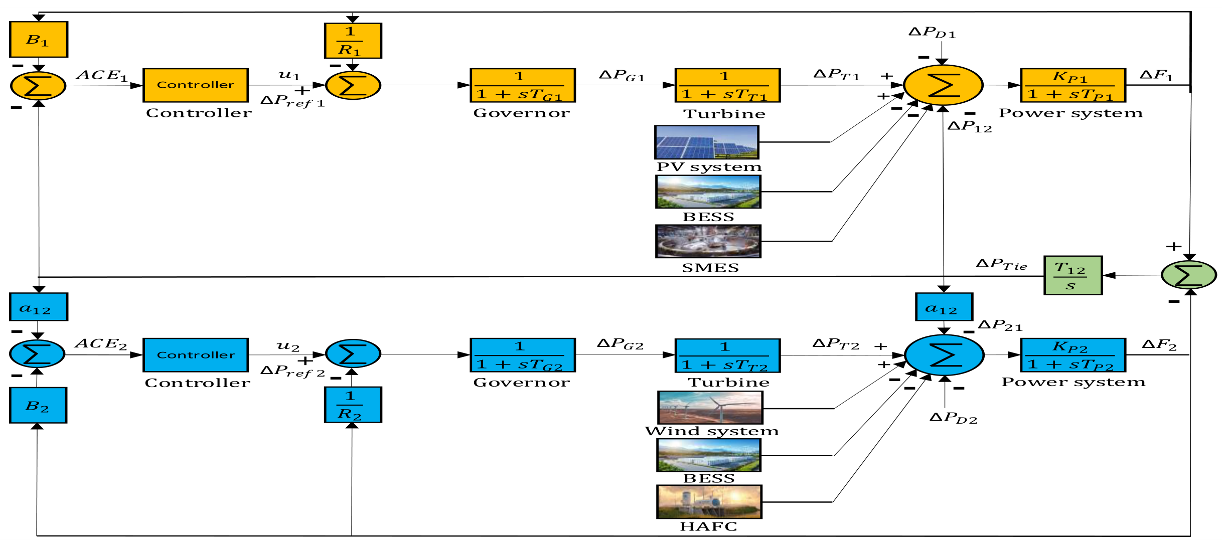
  • Energy storage integration: the measured benefit of VRFB/SMES (Area 1) and VRFB/HAFC (Area 2) is quantified across all scenarios and showed the improvement in system’s performance that exposed to fluctuations in frequency due to the intermittent nature of solar and wind.
  • Validation of the aforementioned cases with OPAL-RT simulator: the PS is experimentally analyzed through the OPAL-RT simulator to ensure the validation of numerical simulation by integrating the fidelity of physical simulation with the adaptability of the numerical simulation.
This paper is organized as follows: Section 2 presents the dynamic model of test system. Section 3 presents the proposed TDn(1+PIDn) controller. Section 4 provides the optimization technique, PKO and objective function. Section 5 shows the results. Lastly, Section 6 presents the conclusions.

2. Dynamic Model of Test System

2.1. Two-Area Power System

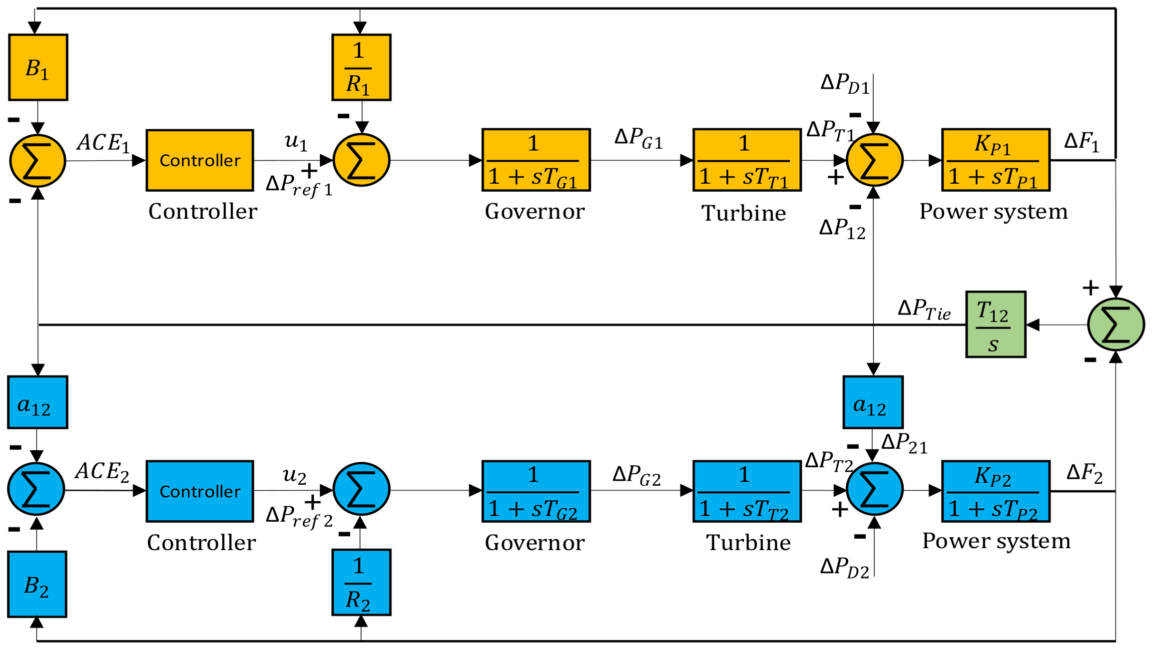
A two-area interconnected non-reheat thermal–thermal PS (case 1) is adopted, as illustrated in Figure 1. This configuration is widely used in [51,52,53] for the study of the dynamic behavior of interconnected systems under both steady-state and transient operating scenarios. Each area has generating units with a total installed capacity of 2000 MW, operating at a nominal base load of 1000 MW. Both areas incorporate conventional control components, including a speed governor, a non-reheat steam turbine, and PS units. Nominal values of the model parameters are from [51,52] and are presented in Table 2. The nonlinear turbine model shown in Figure 2, which incorporates a GRC with limits of α = ±0.05 pu/s and α = ±0.025 pu/s, replaces the linear non-reheat turbine transfer function of Figure 1 to account for the physical ramp-rate limitation of the steam turbine under realistic operating conditions. The GDB represents a nonlinear characteristic of the governor system, defining a range of frequency deviations within which no corrective valve action is initiated. This behavior originates from mechanical valve-positioning tolerances and intentional filtering mechanisms designed to limit unnecessary actuator movements. Consequently, the governor response exhibits an inherent delay that may increase phase lag and reduce the effectiveness of LFC. To account for this practical nonlinearity, the GDB is incorporated into the governor model through a modified transfer function, expressed as ( 0.2 / π s + 0.8 ) / ( T G s + 1 ) , which replaces the linear governor transfer function of Figure 1, allowing for a more realistic representation of valve dynamics under small frequency variations [27,54,55]. In addition, CTD is a characteristic of modern wide-area LFC systems due to the use of communication networks.
This delay is associated with the transmission of measured system variables to the control center and the subsequent delivery of control signals to generation units. Following a load disturbance, these communication lags affect the timely generation and execution of corrective control actions, thereby affecting the performance of the PS. To account for this practical nonlinearity, the CTD is incorporated into the overall plant model after the controller in Figure 1 using the exponential function e s τ , where τ denotes the communication delay time, considered to be 0.1 s. This representation enables a more realistic assessment of system dynamics and controller performance under networked operating conditions [55].
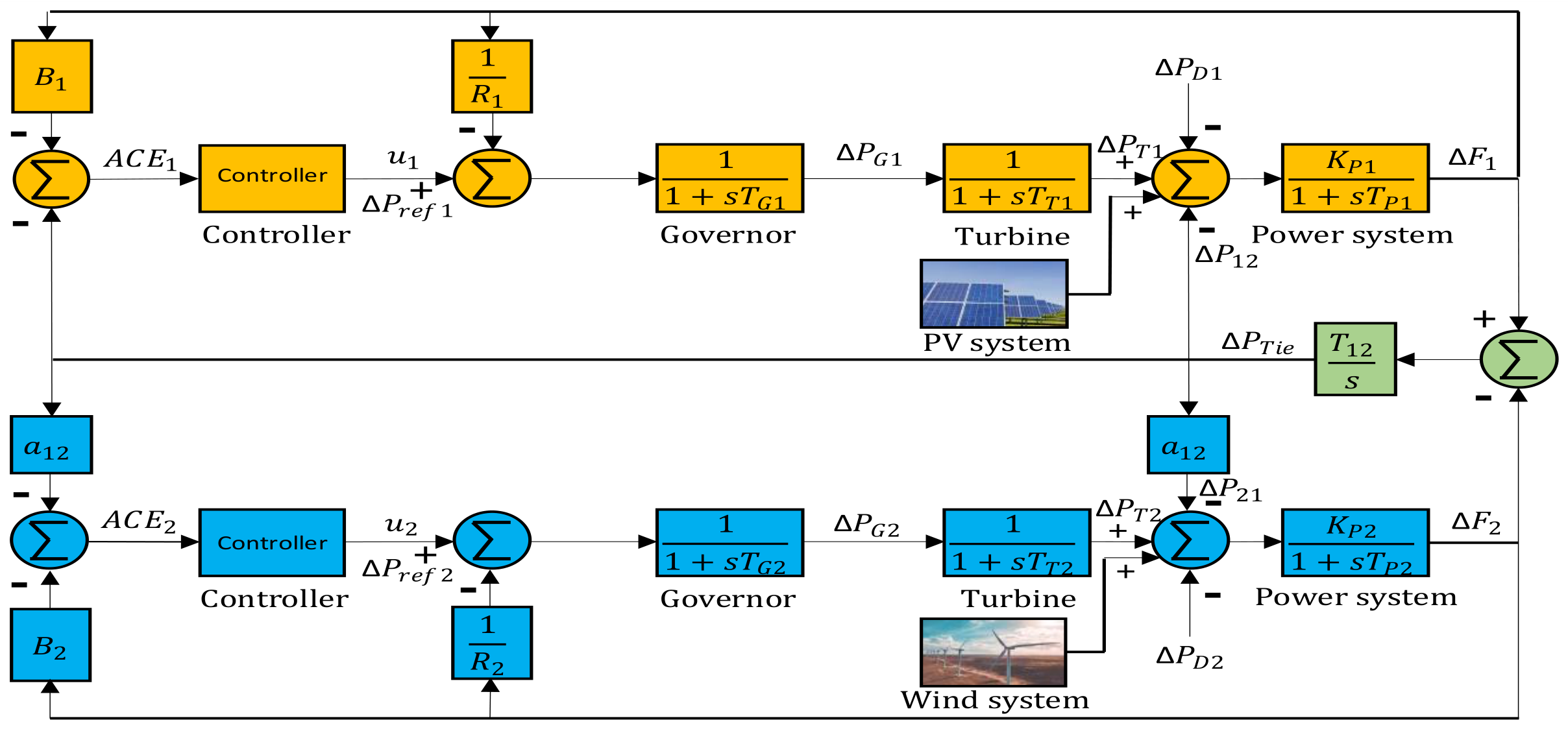
RESs are added to the PS for environmental and economic aspects; therefore, PV in area 1 and WT in area 2 (case 2) are adopted, as illustrated in Figure 3. To mitigate the fluctuations resulting from RESs, ESSs are added to PS; therefore, VRFB and SMES in area 1 and VRFB and HAFC in area 2 (case 3) are adopted, as illustrated in Figure 4. The transfer function of the governor G G s , turbine G T s , and generator G P s are represented as follows [56]:
G G s = Δ P V ( s ) Δ P G ( s ) = 1 1 + s T G .
The speed governor has two inputs, Δ P r e f s and Δ F , with one output, Δ P G s , given by:
Δ P G s = Δ P r e f s 1 R Δ F   ( s ) ,
G T s = Δ P T ( s ) Δ P V ( s ) = 1 1 + s T T ,
G P s = K P 1 + s T P ,
where K P = 1 / D and T P = 2 H / F D .
D is the load frequency dependency parameter given in (5).
D = N o m i n a l   l o a d   ( P D ) N o m i n a l   f r e q u e n c y   ( F ) ,
where T G is the generator time constant, T T is the turbine time constant, K P is the power system gain constant, T P is the power system time constant, P D is the nominal load, H is the inertia constant of the generator, and F is the nominal frequency.
The generator has two inputs, Δ P T s and Δ P D s , with one output, Δ F s , given by:
Δ F s = G P s Δ P T s Δ P D s .
The calculation of area control error (ACE) values for both areas is given in (7) and (8).
A C E 1 = B 1 F 1 + Δ P t i e ,
A C E 2 = B 2 F 2 + Δ P t i e .

2.2. Renewable Energy Sources

2.2.1. PV Model

Uniform Model
The dynamic behavior of PV can be represented using a first-order transfer function, which effectively captures the system’s transient response to variations in irradiance.
Under the assumption of constant ambient temperature, the generated electrical power is linearly correlated with the incident solar radiation. Consequently, the PV system can be modeled as follows [44]:
G P V s = K P V 1 + s T P V ,
where K P V denotes the photovoltaic system gain constant, and T P V represents the photovoltaic system time constant reflecting the PV module’s response delay.
This simplified linear model enables analytical control design and stability analysis of the PV-integrated PS. Table 3 shows the values of these parameters [44].
Random Model
PV exhibits power variability owing to fluctuations in solar radiation and ambient temperature.
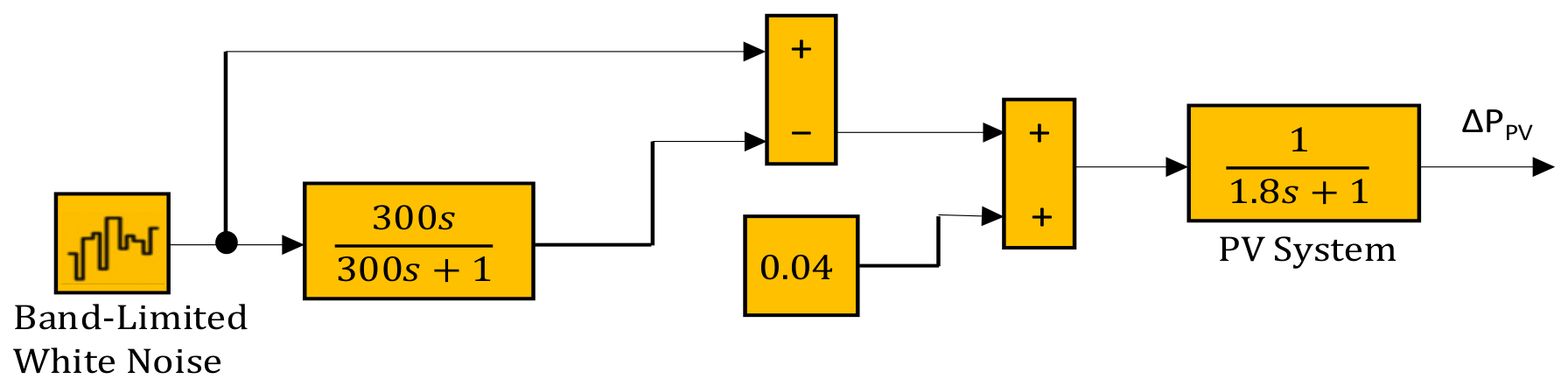
To accurately emulate this dynamic behavior in simulation studies, random power models are typically adopted to represent the temporal variability in PV output. PV generation, as depicted in Figure 5, employs a stochastic model adapted from [45] corresponding to a 6 MW solar facility. The dynamic behavior of the PV plant can be expressed through a first-order transfer function [45], where Δ P S o l a r characterizes the variance in PV output power.
Δ P P V = K P V 1 + s T P V Δ P S o l a r .

2.2.2. WT Model

Uniform Model
The dynamic performance of WT can be approximated using a first-order transfer function that characterizes the system’s response to variations in wind speed. Under the assumption of uniform air density and negligible mechanical losses, the electrical power generated by the turbine is directly proportional to the cube of the effective wind velocity. Accordingly, the transfer function of the WT can be represented as follows [44]:
G W T s = K W T 1 + s T W T ,
where K W T denotes the wind system gain constant, and T W T represents the wind system time constant reflecting the WT’s response delay. This simplified linear model enables analytical control design and stability analysis of WT-integrated PS. Table 3 shows the values of these parameters [44].
Random Model
With the growing urgency to address global energy sustainability, RESs have gained significant attention, with wind power emerging as a major contributor to modern power systems. In this study, a 5 MW offshore WT model developed by the National Renewable Energy Laboratory (NREL) under the Wind Energy Technologies Programme of the U.S. Department of Energy was utilized. This model is widely recognized as a benchmark for offshore WT research, design optimization, and performance evaluation across diverse operating conditions. The 5 MW capacity represents the industry standard for large-scale offshore turbines, ensuring compatibility with international modeling frameworks and cost-efficiency analyses. Due to the substantial infrastructure and installation costs associated with deep-water deployment, turbines in this category generally possess ratings of 5 MW or higher to achieve favorable economic performance [57,58,59].
The effectiveness of wind energy generation primarily depends on the transformation of wind’s kinetic energy into electrical energy. This process starts with the turbine blades capturing the kinetic energy of the wind and converting it into mechanical energy at the rotor shaft. Mechanical energy is subsequently transformed into electrical energy through the generator unit. The total aerodynamic power extracted from the wind can be calculated from (12)–(15) [60,61].
P W i n d = 1 2 . ρ . A T . V 3 . C P λ T , β ,
C P λ T , β = C 1 C 2 λ 1 C 3 β C 4 β 2 e C 5 λ 1 + C 6 λ T ,
1 λ 1 = 1 λ T + 0.08 β 0.035 β 3 + 1 ,
λ T = V T P V = R ω r V ,
where P W i n d represents the wind turbine power, A T is the swept area of the turbine, V is the wind speed, ρ is the air density, C P is the turbine performance coefficient, β is the blade pitch angle, λ T is the tip speed ratio, λ 1 is the effective tip speed ratio, V T P is the tip speed, R is the blade radius, and ω r is the rotor speed. C P represents a nonlinear function that depends on both the aerodynamic configuration of the turbine blades and the operational conditions of WT. It characterizes the conversion efficiency by which the kinetic energy of the wind is transformed into mechanical energy.
The coefficients C 1 through C 6 are determined by the blade’s shape and its aerodynamic properties. Notably, the turbine attains its maximum power output when the blade pitch angle β equals zero degrees, corresponding to the optimal aerodynamic alignment.
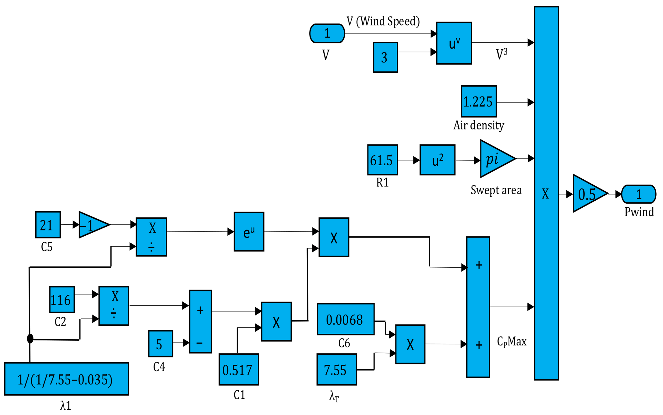
The technical specifications of the 5 MW NREL wind turbine model are taken from [45,60,62,63]. The radius of the swept area (R1) is 61.5 m, while the rotor diameter (D) is 126 m and the hub diameter (DH) is 3 m. The rotor operates at a speed (ωr) of 12.1 rpm. The cut-in wind speed (Vin) is 3 m/s, whereas the rated wind speed (V) reaches 11.4 m/s. The air density (ρ) is taken as 1.225 kg/m3. In addition, the optimal tip-speed ratio (λT) is 7.55. The power coefficient constants (C1–C6) are given as 0.517, 116, 0.4, 5, 21, and 0.0068, respectively.
The maximum power of the NREL- 5 MW WT can be evaluated using (16)–(18).
C P _ m a x = C P λ T = 0.517 116 λ 1 5 e 21 λ 1 + 0.0068 λ T ,
1 λ 1 = 1 λ T 0.035 ,
P W i n d _ m a x = 1 2 . ρ . A T . V 3 . C P _ m a x .
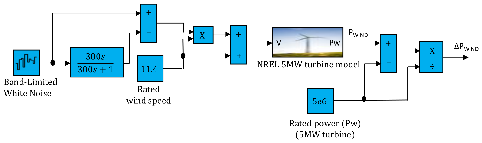
A model of fluctuating WT for frequency control is shown in Figure 6. The random wind power is obtained by multiplying the wind speed standard deviation by the random output fluctuation from the white noise block [23,64,65]. Figure 7 shows the WT model of the NREL 5 MW with maximum power generation [62].

2.3. Energy Storage Systems

2.3.1. Vanadium Redox Flow Battery Model

VRFBs emerge as an encouraging large-scale energy storage system within renewable power systems owing to their high energy density, long cycle life, and rapid response features.
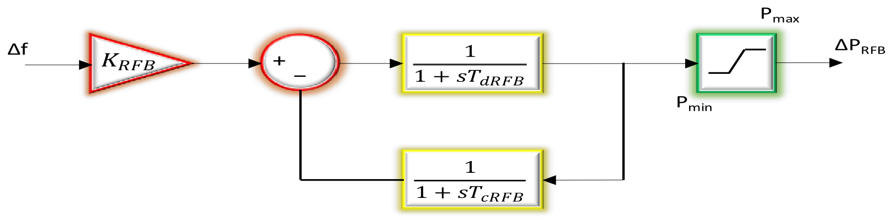
These attributes make VRFBs particularly suitable for mitigating fluctuations and enhancing overall grid reliability and stability. The transfer function of the VRFB employed for load frequency control is illustrated in Figure 8. In this model, KRFB denotes the vanadium redox flow battery gain constant, while TdRFB is the vanadium redox flow battery time delay constant, and TcRFB is the resetting vanadium redox flow battery time constant. Table 4 shows the values of these parameters. This transfer function-based formulation provides an analytically tractable means of characterizing the electrochemical–dynamic behavior of the battery within load frequency control frameworks [66]. It reproduces the dominant charge and discharge response relevant to frequency support, but it does not capture the accurate electrochemical behavior or the battery’s state of charge. Richer electrochemical and state-of-charge estimation methods, of the kind surveyed in [67], would support a more detailed handling over long regulation terms.

2.3.2. Super Magnetic Energy Storage Model

SMES systems are instrumental in maintaining frequency stability within modern power grids. These units regulate system dynamics by supplying or absorbing electrical power as needed by the grid, thereby mitigating frequency deviations and enhancing overall reliability. The transfer function representation of the SMES, as demonstrated in Figure 9, is developed using a two-stage lead–lag compensator structure [68]. In this model, T1, T2, T3, and T4 denote the lead-lag blocks time constants. The parameter KSMES is the super magnetic energy storage gain constant, and TSMES defines the super magnetic energy storage time constant. Table 4 shows the values of these parameters.

2.3.3. Hydrogen Aqua Electrolyzer Fuel Cell Model

Hydrogen-based energy conversion systems are increasingly recognized as key enablers of sustainable power generation, offering a viable pathway to reduce reliance on fossil fuels.
Among these systems, the integration of HAFC into hybrid PS has proven effective in enhancing grid frequency regulation and power quality. In such arrangements, surplus renewable electricity is converted into hydrogen through electrolysis, stored for extended periods, and later reconverted to electrical energy by the fuel cell. This closed-loop process enables more flexible utilization of renewable resources and contributes to system reliability. Beyond its operational role, the HAFC architecture delivers multiple advantages, including reduction in greenhouse gas emissions, improved energy recovery, and reduced maintenance costs, with reported round-trip efficiencies typically ranging between 20% and 40% [69].
Within a hybrid renewable framework, the power generated by RESs is dynamically balanced through coordinated operation of the electrolyzer and fuel cell components to sustain the overall system equilibrium. To capture the HAFC’s dynamic behavior, the coupled electrolyzer–fuel cell structure can be reasonably approximated using a first-order transfer function model.
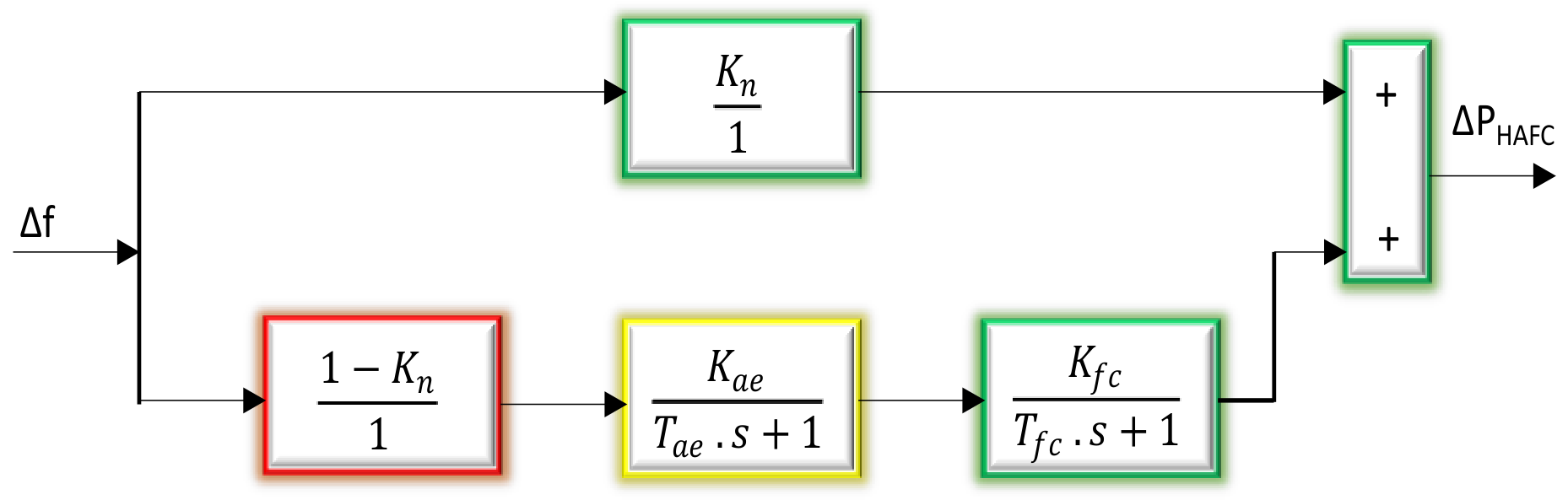
In this study, power fluctuation is used as the input disturbance driving the HAFC response, as shown in Figure 10 [70]. The transfer function of HAFC is expressed in (19).
Δ P H A F C = K f c T f c . s + 1 · K a e T a e . s + 1 · 1 K n 1 + K n · Δ F ,
where K f c and T f c define the gain and time constants of fuel cell, and K a e and T a e correspond to the gain and time constants of aqua electrolyzer. K n is a conversion factor that equals
K n = P H 2 P W T + P P V ,
and is assumed to be 0.6, where P H 2 defines the power output from the hydrogen fuel cell, P W T is the power generated from WT, and P P V is the power generated from PV.
The HAFC is captured by a coupled first-order electrolyzer–fuel-cell model that reproduces the fast, bounded power exchange relevant to the LFC problem. This representation omits the reversible voltage loss and the recovery that follows it; both affect efficiency and durability over longer terms [71]. Additionally, this representation does not resolve the internal thermal field of the stack. In a physical PEMFC, the speed at which power can be ramped is tied to the temperature distribution across the membrane and to the effectiveness of the cooling circuit; so, a rapid regulation command may be followed by a short thermal-inertia lag before the electrical output fully settles. The recent review of liquid-cooled PEMFC thermal management by Song et al. [72] sets out these effects and the associated control challenges in detail. Coupling the electrical model with a thermal-management sub-model would give a more faithful account of the achievable ramp rate and of the long-term efficiency and service life of the stack.

3. Proposed Multi-Stage Controller

The proposed TDn(1+PIDn) control strategy is designed to enhance the dynamic performance of interconnected PS in LFC applications [43]. Accurate frequency regulation is crucial to maintaining the stability and reliability of modern grids under varying load profiles and renewable energy variations. By integrating a nonlinear tilt-derivative component with a filtered PID block, the controller achieves improved stability, reduced overshoot, and faster transient response under varying operating conditions. The coordinated interaction between both control stages enables superior robustness against external disturbances and parameter uncertainties.

3.1. TDn Controller

The TDn section represents an advanced derivative element that incorporates a nonlinear tilt function and an n-filter. Unlike conventional derivative terms that rely solely on the rate of change of the error signal, the TDn introduces nonlinear dynamics into the derivative path. This modification enhances the controller’s responsiveness to rapid frequency deviations in the PS, enabling faster corrective actions and improved damping of transient oscillations. Moreover, the filter effectively mitigates the noise amplification problem often observed in conventional derivative terms, thereby reinforcing the overall robustness and stability of the load frequency control system under fluctuating grid conditions.

3.2. PIDn Controller

The PIDn section integrates proportional, integral, and derivative control actions, each enhanced with an n-filter to suppress noise and maintain stability. In load frequency control applications, this nonlinear configuration enables adaptive tuning under diverse operating conditions. It ensures effective mitigation of transient frequency deviations, accurate steady-state regulation, and overall improvement in system reliability and power balance.

3.3. Interaction Between TDn and PIDn

The coordinated operation of the TDn and PIDn sections enables effective control of both transient and steady-state frequency deviations. The TDn part ensures rapid stabilization following load disturbances and RES fluctuations, while the PIDn section refines the response to maintain frequency near its nominal value. Their combined action strengthens system stability and robustness against uncertainties in load frequency control applications.

3.4. Multi-Stage Structure

The proposed TDn(1+PIDn) controller introduces a multi-stage configuration that markedly enhances the stability and dynamic response of interconnected PS under load and RES fluctuations. This architecture allows for progressive refinement of control actions across distinct operating phases, enabling precise frequency regulation and improved adaptability to nonlinear system dynamics. The initial control phase focuses on rapid frequency restoration, mitigating transient deviations and suppressing oscillations resulting from sudden load or RES disturbances. Subsequently, the intermediate correction phase ensures smooth transitional behavior by addressing moderate deviations and nonlinearities within the PS. The final stage provides high-accuracy steady-state regulation, reducing residual frequency errors and maintaining long-term system stability even under persistent disturbances.
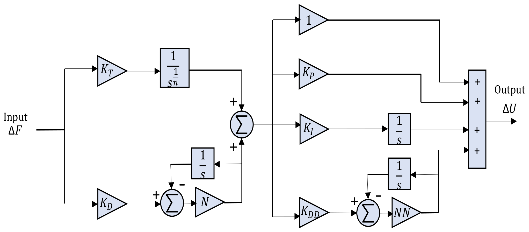
By integrating these stages, the TDn(1+PIDn) scheme achieves an optimal compromise between responsiveness and robustness. Its adaptive characteristics allow for consistent performance across a wide range of operating conditions, outperforming conventional controllers such as PID, the common configuration. This advanced design not only strengthens the frequency restoration capability but also improves tie-line power regulation, making the proposed controller particularly suitable for modern hybrid PS where renewable integration introduces strong nonlinearities and dynamic uncertainties. The block diagram of the proposed controller is shown in Figure 11.
The open-loop transfer function for the first-stage controller is as follows:
G T D n s = Δ U 1 s Δ F s = K T s 1 n + K D N s N + s .
The open-loop transfer function of the second stage controller is given in (22).
G ( 1 + P I D n ) s = Δ U s Δ U 1 s = 1 + K P + K I s + K D D N N s s + N N .
In order to explain the open-loop representation of the proposed controller, (23) can be formulated as follows:
G T D n ( 1 + P I D n ) s = Δ U s Δ F s = K T s 1 n + K D N s N + s 1 + K P + K I s + K D D N N s s + N N ,
where K D , K D D , K P , and K I are the derivative, proportional and integral gains of controller, while N , N N , and n are the controller filters.

3.5. Frequency-Domain Interpretation of the Proposed Controller

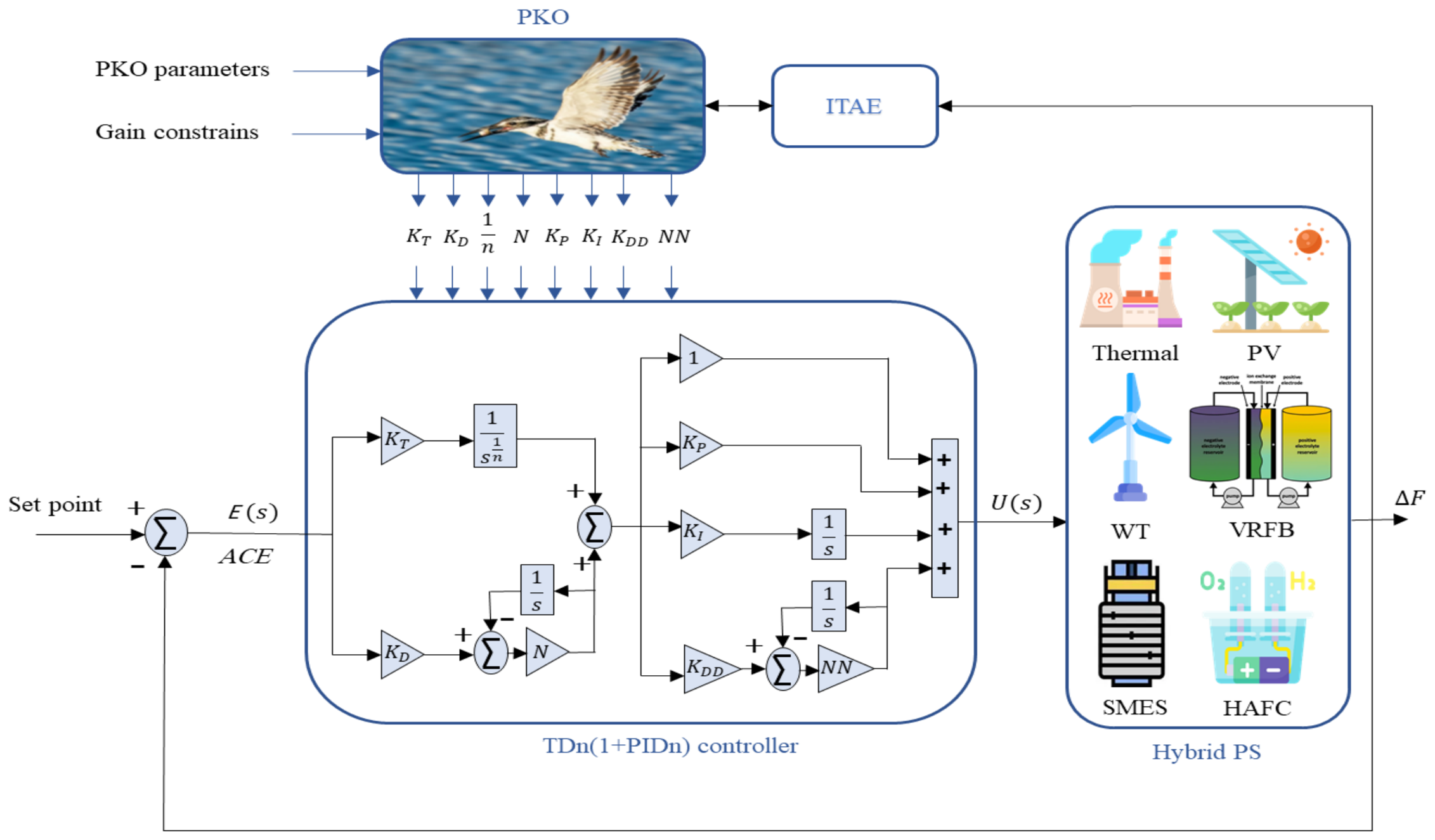
To move beyond empirical demonstration and provide a mechanistic explanation for the performance gains achieved by the proposed structure, the open-loop characteristics of each stage are examined in the frequency domain. The TDn stage operates through two complementary elements: the tilt element K T / s ^ ( 1 / n ) introduces a fractional-order gain slope at low frequencies, enhancing attenuation of slow-varying disturbances such as sustained load perturbations and gradual renewable power fluctuations, while the filtered derivative element K D N s / ( N + s ) injects phase advancement in the mid-frequency band, enabling rapid suppression of transient deviations before they propagate further; the filter N simultaneously prevents amplification of high-frequency measurement noise. The succeeding (1+PIDn) stage operates on the pre-shaped signal to accomplish steady-state and bandwidth objectives: the integral action eliminates residual steady-state error, the proportional gain governs the closed-loop bandwidth, and the filtered derivative contributes additional damping without reintroducing the noise attenuated upstream, while the direct unity feed-through path preserves the frequency content already shaped by the TDn stage. The structural consequence of this two-stage arrangement is that fast transient shaping and precise steady-state correction are assigned to dedicated stages operating in complementary frequency bands, a functional separation that a single conventional PID structure cannot achieve simultaneously. Table 5 summarizes the optimal parameters and ITAE values of the proposed and benchmark controllers, all obtained on the identical two-area non-reheat thermal test system under the same parameters and conditions. Beyond PID-family controllers, the comparison includes advanced fractional-order and multi-degree-of-freedom designs from recent research, specifically a DSA-tuned FOPID and WOA-tuned 2DOF-TIDF and TIDF, and other optimization techniques with fuzzy PI controllers. Additionally, a framework of the hybrid PS, the proposed controller in two-area system, the optimization method, and the objective function studied in this research is shown in Figure 12.

4. Optimization Technique and Objective Function

4.1. Optimization Technique

The PKO is a recently introduced swarm-based metaheuristic inspired by the unique hunting strategies and cooperative interactions of pied kingfishers in their natural environment [47].
The algorithm is organized into three functional phases: (1) perching/hovering for prey (exploration/diversification), (2) diving for prey (exploitation/intensification), and (3) fostering symbiotic relations. These biological behaviors are mathematically modeled to navigate complex and high-dimensional search spaces effectively.
To validate its robustness and adaptability, the PKO has been benchmarked against thirty-nine test functions covering unimodal, multimodal, hybrid, and composite landscapes. Moreover, its capabilities are further demonstrated through application to eight real-world engineering design problems, including both constrained and unconstrained formulations.
The overall results emphasize PKO’s strong capability in handling complex optimization tasks involving difficult and diverse search landscapes. The algorithm shows a well-balanced approach between exploration and exploitation, enabling it to efficiently navigate the search space while minimizing the risk of becoming trapped in local optima.
As with many population-based optimization techniques, the PKO begins by randomly generating an initial set of candidate solutions across the search space. This initial population serves as the algorithm’s first exploration trial. The initialization of each solution is performed using (24).
X i , j = L B + U B L B × r a n d ,   i = 1 ,   2 , , N   a n d   j = 1 ,   2 , ,   D i m ,
where X i , j refers to the location of the ith individual at the jth dimension, rand is a uniformly distributed random number in the range [0, 1], and L B and U B represent the lower and upper bounds of the search space, respectively. After generating the initial population, a fitness function is applied to measure the quality of each candidate based on its ability to address the given optimization task. Individuals with the best fitness values are selected to produce a new generation.

4.1.1. Exploration Phase

The exploration phase of PKO is inspired by the perching and hovering strategies observed in pied kingfishers during foraging. Field studies show that these birds alternate between launching attacks from stationary perches and from mid-air hovering, depending on environmental and situational factors. In the context of PKO, these natural behaviors guide how search agents explore the solution space. Each agent’s position is dynamically adjusted based on this biologically inspired foraging mechanism, and the positions are updated in (25).
X i t + 1 = X i t + α T ( X j t X i t ) ,             i , j = 1 ,   2 , , N   a n d   j     i .
During the iterative update process, the position of a search agent in the next iteration is expressed as X i t + 1 , while X i t represents its current location. The parameter α is computed as 2 r a n d n 1 , D i m 1 , where r a n d n represents a random number from a normal distribution. N denotes the population size, and D i m signifies the dimensionality of the problem under consideration. The parameter T is a key component in our approach, with its value adaptively changing according to the current behavioral strategy, either perching or hovering. The calculation of T is specifically designed to align with the characteristics of each strategy, enabling efficient operation in different system modes.
Perching
Pied kingfishers are known to initiate hunting by perching on elevated natural or artificial structures such as trees, rocks, or utility lines, from which they scan nearby water bodies for signs of prey. Initially, they rely on monocular vision to survey a broad area and detect subtle movements on the water’s surface. Upon identifying a potential prey, they switch to binocular vision to accurately judge distance and lock onto the prey, allowing for precise and well-timed capture movements.
However, the crest angle of a pied kingfisher can also influence its hunting dynamics. The perching mechanism can be mathematically modeled as previously described in (25) and the T parameter can be calculated as follows:
T = ( exp 1 exp t 1 M a x I t e r 1 B F ) c o s ( C r e s t a n g l e s ) ,
c r e s t a n g l e s = 2 p i r a n d .
The maximum number of iterations is specified by M a x I t e r . The constant value B F , beating factor, is set to 8, and r a n d is a random value between 0 and 1.
Hovering
The pied kingfisher can hover in place due to its fast and powerful wing beats. Its wings, though relatively short and broad, are built to beat at a high frequency, keeping the bird steadily suspended in the air. Unlike many other birds, its long and pointed wings create enough lift to support this hovering behavior. The hovering strategy can be mathematically expressed as previously given in (25) and the T parameter can be calculated as follows:
T = b e a t i n g r a t e t 1 B F M a x I t e r 1 B F ,
b e a t i n g r a t e = r a n d P K O F i t n e s s j P K O F i t n e s s i .
The fitness of the ith and jth pied kingfishers is represented by P K O F i t n e s s ( i ) and P K O F i t n e s s ( j ) , respectively. As it is a constant value, B F , the beating factor, is set to 8.

4.1.2. Exploitation Phase

The pied kingfisher exhibits exceptional precision in diving behavior. During hunting, the bird perches above water to locate prey, and then performs a rapid, high-angle dive to capture fish held in its beak with remarkable accuracy. This natural behavior embodies a balance between exploration (searching from elevation) and exploitation (targeted diving toward the prey), which is abstracted into the PKO algorithm’s search dynamics. The beak’s optimized shape, due to its strength and precision, have also influenced modern engineering designs such as reducing the noise of bullet trains and realizing efficient underwater vehicles, reinforcing the kingfisher’s relevance as a model for intelligent and adaptive optimization strategies. The mathematical representation is presented in (30)–(33):
X i t + 1 = X i t + H A o α b X b e s t t   ,           i = 1 ,   2 , , N ,
H A = r a n d P K O F i t n e s s i B e s t F i t n e s s ,
o = e x p t M a x I t e r 2 ,
b = X i t + o 2 r a n d n X b e s t ( t ) ,
where B e s t F i t n e s s represents the best fitness value obtained over all iterations, α is a control parameter, calculated as follows: r a n d n 1 , D i m 1 ; o and H A denotes the hunting ability.

4.1.3. Commensalism Phase

The pied kingfisher exhibits adaptive hunting behavior influenced by environmental and ecological factors such as prey availability and competition. It often forms a commensal association with otters, benefiting from fish disturbed during otter activity. This cooperative interaction enhances its hunting efficiency without mutual harm. In PKO, this ecological relationship is abstracted as the commensalism or local escape phase, enabling candidates to share information and refine their positions through cooperative learning for improved local search efficiency. This behavior is mathematically presented as follows:
X i t + 1 = X m t + o . α . | ( X i t X n t ) |   i f   r a n d > ( 1 P E ) X i t o t h e r w i s e ,
i = 1 ,   2 , , N ,
o = e x p t M a x I t e r 2 ,
α = 2 r a n d n 1 , D i m 1 ,
P E = P E m a x P E m a x P E m i n t M a x I t e r .
Two individuals, denoted as X m and X n , are randomly selected from the population to model the local interaction behavior. The predatory efficiency ( P E ) parameter controls this interaction, bounded within P E m i n = 0 and P E m a x = 0.5, to regulate the adaptive balance between exploration and exploitation in the search process.
The algorithm iterates through these steps until the maximum number of iterations is reached, continuously updating the best solution. Finally, once the termination criteria are met, the algorithm returns the optimal solution found.
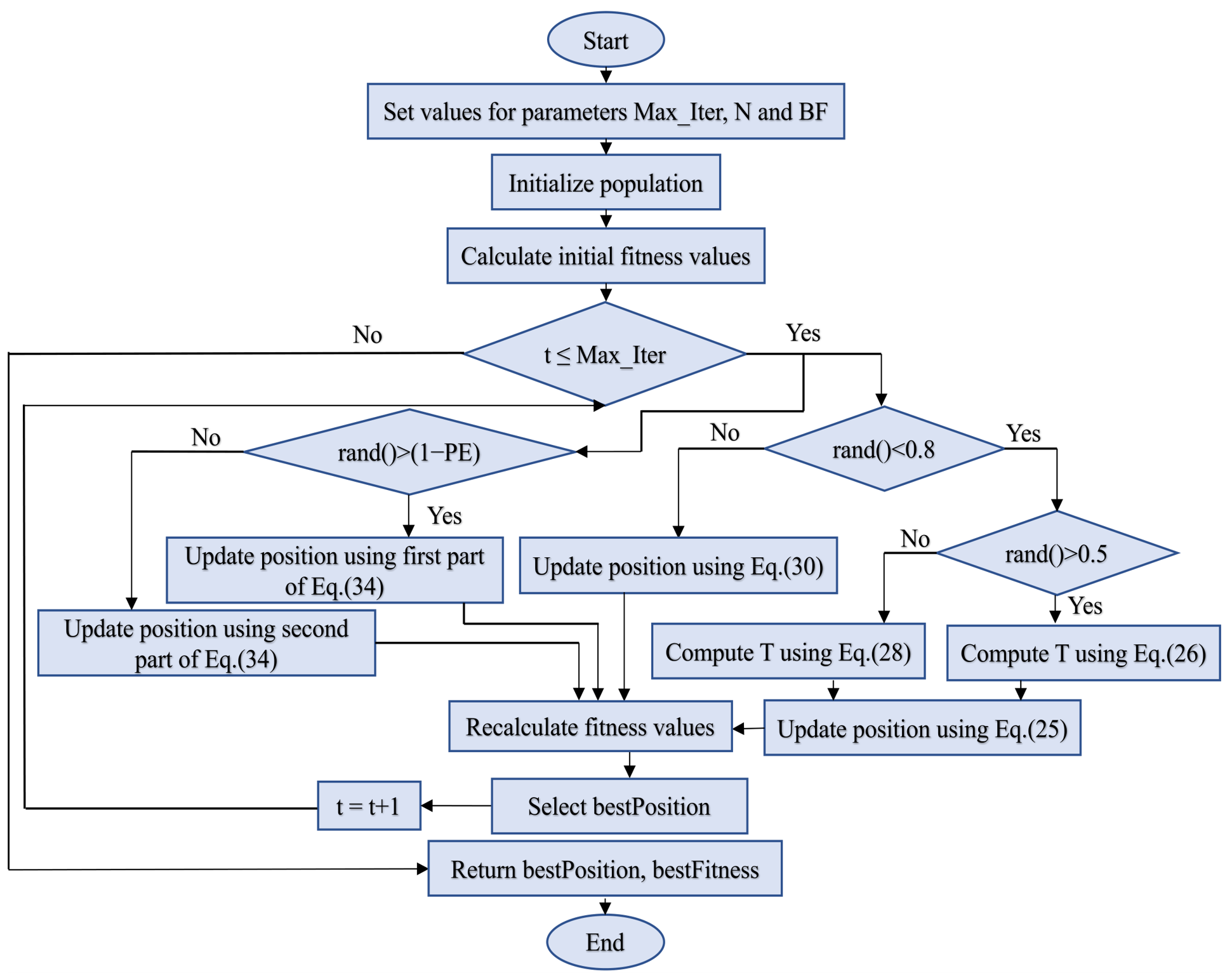
Substantially, the PKO algorithm balances exploration and exploitation through the perching, hovering, diving phase, and commensalism phase, where the first two drive broad global search via dynamically scaled stochastic updates, the diving phase intensifies local refinement toward the optimal solution through a fitness-weighted step mechanism, and the commensalism phase actively prevents local optima entrapment by probabilistically relocating stagnating agents across the population. This structured transition from exploration to exploitation, governed by adaptive parameters that evolve with iteration progress, overcomes the premature convergence and local optima susceptibility inherent in PSO and GWO, enabling PKO to achieve superior convergence accuracy and solution quality in the high-dimensional, multimodal parameter search space characteristic of the LFC controller tuning problem addressed in this work. Figure 13 represents the flowchart of procedural stages of the proposed PKO.

4.2. Objective Function

The objective function (OF) serves as a quantitative measure for evaluating the dynamic performance of the PS and the effectiveness of the proposed method. It ensures that the controller output maintains optimal performance under varying conditions while minimizing steady-state error. In this study, the parameters of the TDn(1+PIDn) controller are optimized using the PKO algorithm to mitigate frequency and tie-line power oscillations in PS that include RESs and ESSs. Accordingly, ITAE is employed as the objective function, expressed as follows [75]:
O F I T A E = 0 t s i m F 1 + F 2 + P t i e . t . d t .
In the above Equation, F 1 and F 2 are the system frequency deviations in area 1 and area 2, respectively. P t i e is the incremental change in tie line power, and t and t s i m are the present and simulation times.
To keep the comparison fair, PSO, GWO and PKO were run under matched conditions: population size (30), number of iterations (50), the same gain bounds from Table 6, the same ITAE objective function in (39), and number of independent runs (20), with every run facing the same disturbance and renewable sequences and conditions. PSO used an inertia weight w initialized at 1 and damped multiplicatively by a factor of 0.99 per iteration, together with a personal learning coefficient c 1 = 1.5 and a global learning coefficient c 2 = 2, and GWO used the convergence coefficient a decreasing linearly from 2 to 0 with iteration [76]. PKO’s own parameters, a beating factor ( B F ) of 8 and a predatory efficiency ( P E ) range from 0 to 0.5 for the commensalism phase, were taken directly from the original paper [47] and left unchanged; so, no technique received a tuning advantage. Because a single realization of a stochastic optimizer carries little weight on its own, each algorithm was executed over these twenty independent runs and its performance judged on the distribution of outcomes rather than on any one trajectory. The statistical analysis across the independent runs is reported in Table 7.
The superiority of the proposed PKO-TDn(1+PIDn) method in LFC problem is demonstrated through an extensive comparative analysis with several modern methods for the same test system with identical parameters and conditions, as summarized in Table 6. Table 5 shows that PKO-TDn(1+PIDn) achieves the lowest ITAE value (0.0373) among all evaluated methods, corresponding to reductions of approximately 31% and 33% relative to GWO and PSO with the same controller. The reduction reaches about 49% and 52% relative to WOA-tuned 2DOF TIDF and DSA-FOPID. Relative to the WOA-tuned TIDF, HPSO-PS-tuned fuzzy PI, EPSDE-PID, and CLPSO-PID methods, ITAE reductions are roughly 68%, 74%, 75%, and 76%, respectively. In addition, the proposed method outperforms PSO-tuned fuzzy PI and PS-tuned fuzzy PI methods by more than 91% and 94%, respectively. Consequently, the proposed method exhibits superior transient performance in terms of faster response, lower overshoot, and improved steady-state accuracy.
The controller parameters are optimized subject to predefined bounds to ensure system stability and practical realizability. The admissible limits of the controller parameters are summarized in Table 6. The design problem can be formulated as the following optimization problem.
Minimize O F I T A E subject to:
θ M i n θ θ M a x ,
where θ is vector of controller parameters, and θ M i n , θ M a x are bounds for each controller parameter taken from Table 6.
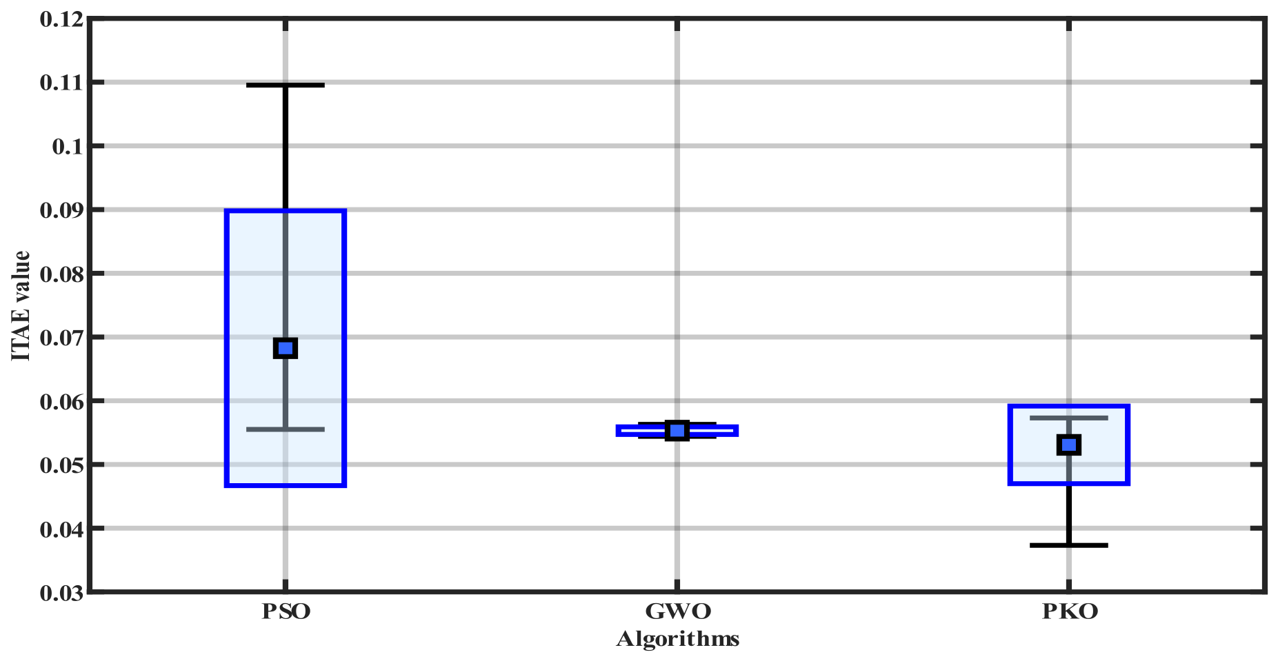
The PKO algorithm was executed in many separate runs, with Table 7 displaying the best, worst, mean, and standard deviation of OF values achieved by different optimization algorithms for the same proposed controller.
The boxplot in Figure 14 of PKO, GWO, and PSO under the proposed controller shows a more compact interquartile range and lower median value for PKO compared with PSO, with GWO lying in between. Such a distribution suggests that PKO not only yields better median performance but also limits the occurrence of outliers, highlighting its capability to avoid poor local minima and maintain stable convergence characteristics.
The PKO algorithm is executed for a sufficient number of iterations to guarantee convergence toward an optimal solution.
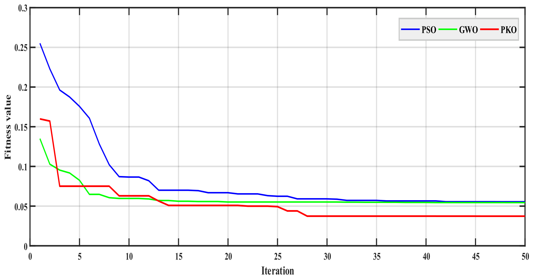
The PKO technique is used to evaluate the effectiveness of the proposed controller. Figure 15 shows that PKO achieves the lowest OF values with a consistently superior convergence rate throughout the optimization process, whereas PSO and GWO stagnate prematurely at higher OF values, confirming PKO’s enhanced ability to avoid becoming trapped in local optima and identify more optimal controller parameters compared to its counterparts.

5. Results

In this section, the simulation results and their analysis are shown to assess the overall performance of the suggested controllers and algorithms. For this purpose, all cases are implemented in MATLAB/Simulink 2024b. Optimization algorithms such as PKO, GWO, and PSO are implemented as MATLAB m-files.
For clarity, the load disturbances, nonlinearity sources, renewable profiles, and energy storage types used throughout the results are collected in Table 8.
The random PV/WT profiles are generated using band-limited white noise blocks with a fixed default seed applied uniformly to all controllers, ensuring a controlled and reproducible comparison on the same stochastic realization. The robustness of the proposed controller is evidenced by its consistent superiority across four random-profile scenario combinations spanning random renewable generation, and its simultaneous occurrence.
Each area is regulated by an independent TDn(1+PIDn) block carrying eight optimized parameters, the five gains, K T , K D , K P , K I and K D D , the two measurement-filter coefficients, N and N N , and the fractional filter order, 1 / n , so that sixteen parameters are tuned in total for the two-area plant. The additional parameters of the proposed controller do not translate into a heavy implementation. Once tuned, the controller reduces to a fixed low-order linear block, and its real-time simulation on the OPAL-RT produced no overruns, confirming a small online cost. The number of tunable gains is comparable to the cascade and FOPID designs already listed in Table 5, and the tuning itself is performed automatically by the optimizer within the bounds of Table 6. Set against this limited cost, the accuracy gain is clear.

5.1. Case 1—Scenario 1: Sudden Load Increase in Area 1

In this scenario, a +0.1 pu Δ P D is applied in area 1 at t = 0. The resulting dynamic responses, including F 1 , F 2 , and P t i e , are recorded for system performance assessment.
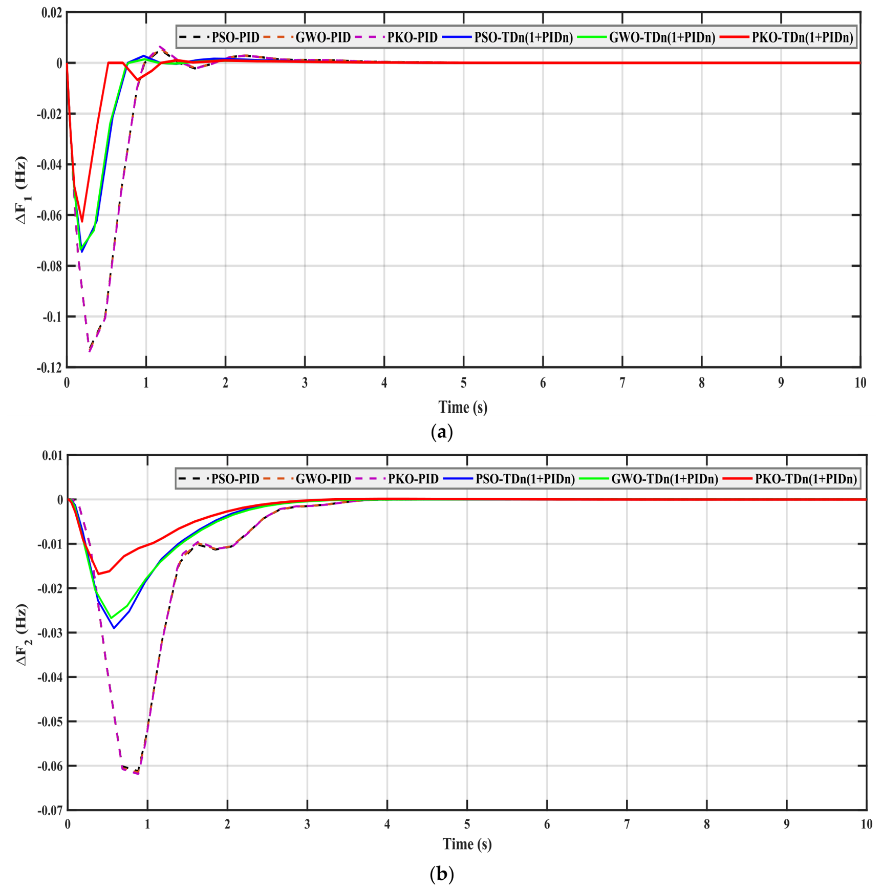
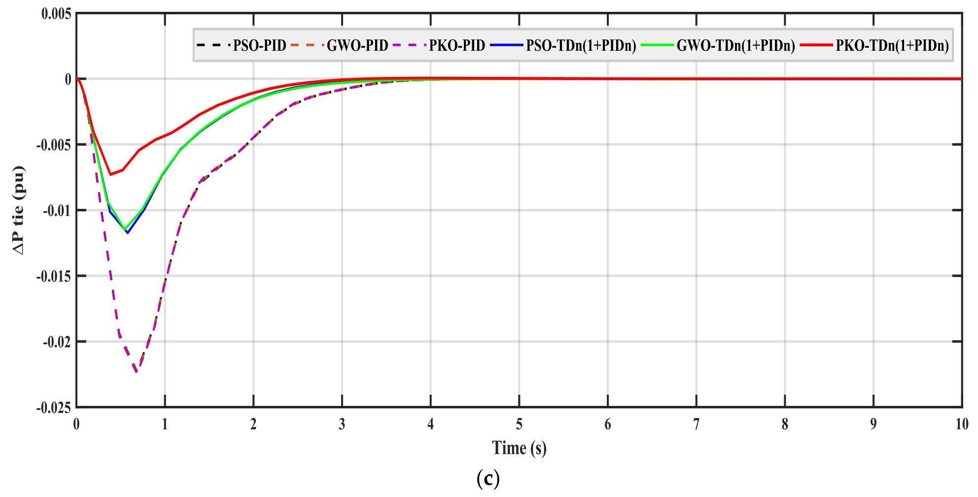
As shown in Figure 16 and Table 9 and Table 10, the PKO-TDn(1+PIDn) controller delivers the strongest overall transient performance as follows: (1) the ITAE reduction from 0.0544 (GWO) and 0.0555 (PSO) to 0.0373 corresponds to 31% and 33% improvement for the multi-stage controller, respectively, and nearly 71% improvement vs. the PID family. (2) For F 1 , undershoot is reduced by 15–16% compared with GWO-TDn(1+PIDn) and PSO-TDn(1+PIDn), and by about 45% relative to PID methods. (3) Overshoot decreases by 28–63% relative to GWO-TDn(1+PIDn) and PSO-TDn(1+PIDn) and 80–84% vs. PID. Its settling time is faster by 7.5% vs. PSO-TDn(1+PIDn) and 26–27% vs. PID. For F 2 , PKO-TDn(1+PIDn) lowers undershoot by 37–42% compared with the other TDn(1+PIDn) designs and by nearly 73% vs. PID, achieving 15–20% shorter settling times. A similar trend appears in P t i e , where undershoot improves by 36–38% relative to other TDn(1+PIDn) and 67% relative to PID, with settling time reduced by 23–25%.
The F 2 and P t i e overshoot values for PKO-TDn(1+PIDn) (1.482 × 10⁻⁴ Hz and 4.85 × 10⁻⁵ pu, respectively) are somewhat higher than the near-zero values recorded for GWO-TDn(1+PIDn) and PSO-TDn(1+PIDn) (of the order of 10−6 Hz and pu), but all three remain extremely small in absolute terms; for PKO-TDn(1+PIDn) itself, the overshoot on each signal is under 1% of the corresponding undershoot; so, the response is, for practical purposes, overshoot-free. Such near-zero values are reported for completeness; the physically meaningful basis for comparison is the undershoot, settling time and ITAE, where PKO-TDn(1+PIDn) shows a consistent advantage across all three signals. Overall, PKO-TDn(1+PIDn) provides the most strongly damped and fastest response among all configurations. The sensitivity analysis shown in Table 11 confirms the strong robustness of the proposed method against realistic power system parameter uncertainty. Under ±25% variation in K P and T P , the controller maintained near-nominal performance, with ITAE deviating by no more than 1.76% from the nominal case and all undershoot, overshoot, and settling-time indices for F 1 , F 2 , and P t i e remaining consistent. This demonstrates the controller’s excellent insensitivity to uncertainties in equivalent generation-side inertia and damping representation. The controller also responded favorably to strengthening of the tie-line coupling ( T 12 + 25%), where ITAE improved by 6.56% relative to nominal, indicating that the design can exploit stronger inter-area synchronization to further enhance frequency regulation.
Even under the more challenging condition of a weakened tie-line ( T 12 − 25%), the controller preserved stable operation and bounded dynamic performance across all indices, without divergence or instability, underscoring the reliability of the PKO-optimized gains across a wide operating envelope.

5.2. Case 1—Scenario 2: Sudden Load Increase in Area 1 with GRC ±0.05, GDB, and CTD 0.1 s in Both Areas

In this scenario, a +0.05 pu Δ P D is applied in area 1 at t = 0. The resulting dynamic responses, including F 1 , F 2 , and P t i e , are recorded for system performance assessment.

5.3. Case 1—Scenario 3: Sudden Load Increase in Area 1 with GRC ±0.025, GDB, and CTD 0.1 s in Both Areas

In this scenario, the setup is the same as in scenario 2, but with a tighter GRC. The resulting dynamic responses, including F 1 , F 2 , and P t i e , are recorded for system performance assessment and compared with scenario 2.
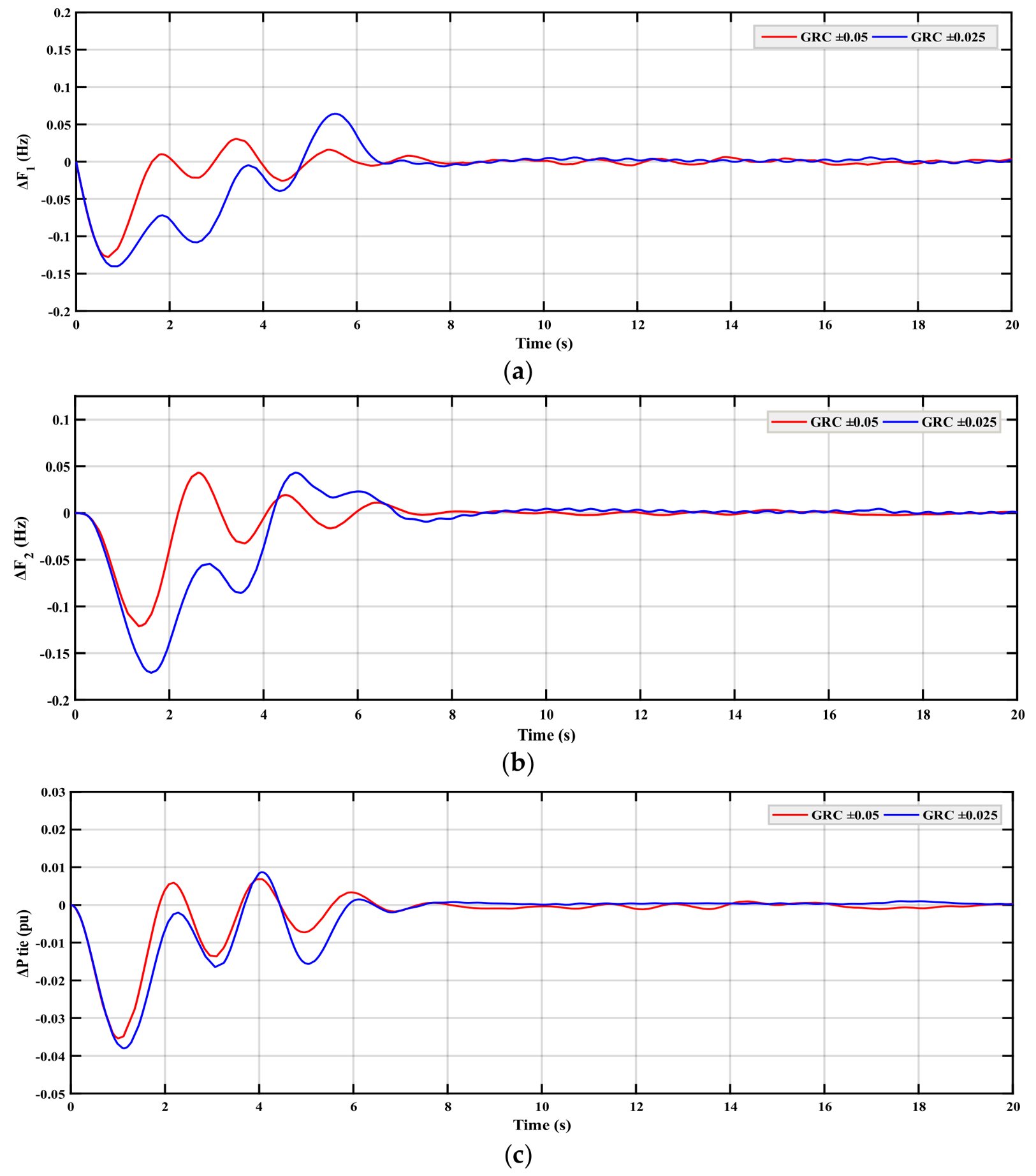
According to Figure 17 and Table 12 and Table 13, the comparison between scenarios 2 and 3 confirms that the GRC exerts a strong effect on LFC performance, even after the GDB and a 0.1 s communication time delay are incorporated into both scenarios to provide a more demanding and realistic test of the proposed method.
With the GRC relaxed to ±0.05, the regulating units are permitted larger ramp rates; so, the system absorbs the disturbance more readily and returns to steady state with smaller deviations and shorter recovery intervals. Constraining the rate to ±0.025 limits how quickly generation can follow the load change, which degrades the dynamic behavior across all three monitored signals.
The undershoots of F 1 , F 2 , and P t i e grow by roughly 9.6%, 41%, and 7.4%, respectively, while their settling times lengthen by about 4.6%, 13.3%, and 13.5%. The overshoot is also affected, rising sharply by close to 109% in F 1 and by about 26.9% in P t i e , whereas the F 2 overshoot stays essentially unchanged. Taken together, these results show that the more permissive ±0.05 limit allows for faster corrective action and yields markedly better damping and overall stability than the tighter ±0.025 constraint. In addition, the results demonstrate that the proposed method decisively overcomes the destabilizing influence of all three nonlinearity sources acting together, GRC, GDB, and CTD, and consistently returns the system to steady state, confirming its effectiveness and reliability under demanding and realistic conditions.

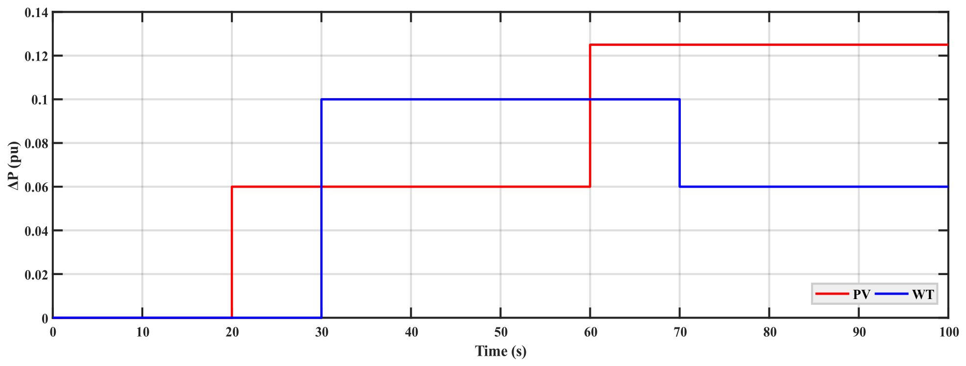
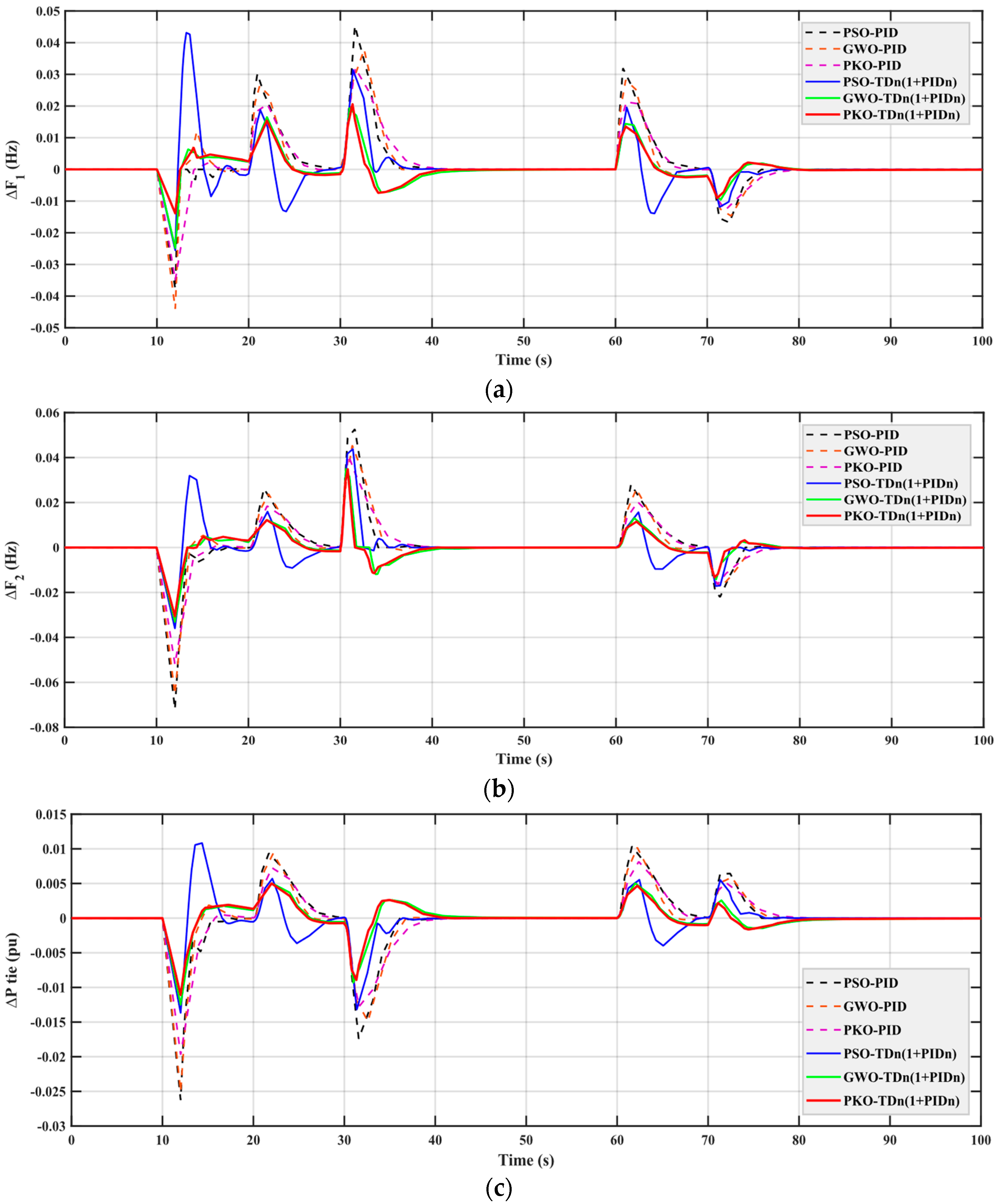
5.4. Case 2—Scenario 1: Fixed Load Increase Under Uniform RES Profiles

In this scenario, a +0.1 pu Δ P D is applied in area 1 at t = 10 s. Area 1 is supplied by PV with a uniform profile, and area 2 is supplied by WT with a uniform profile. The resulting dynamic responses, including F 1 , F 2 , and P t i e , are recorded for system performance assessment and for analyzing the impact of RES penetration in the PS. Figure 18 illustrates the uniform solar and wind power injected into the PS. As shown in Figure 19 and Table 14 and Table 15, the PKO-TDn(1+PIDn) controller provides the strongest overall damping performance. The ITAE reduction from 23.6983 (GWO) and 26.7529 (PSO) to 21.9239 corresponds to 7% and 18% improvement for the multi-stage controller, respectively, and 41% and 46% improvement vs. the PID family. It achieves much smaller undershoot in both F 1 and F 2 , improving by 44–46% compared with the GWO-TDn(1+PIDn) and PSO-TDn(1+PIDn) methods and by 41–68% relative to the entire PID-group. Overshoot behavior also improves in most cases; PKO-TDn(1+PIDn) reduces overshoot in F 2 and P t i e by 20–54% compared with GWO and PSO with the same controller and 23–62% compared with PID-based approaches. A single exception occurs in F 1 overshoot, where it is slightly higher than the GWO-TDn(1+PIDn) value by 6%, but still noticeably better than the PSO-TDn(1+PIDn) and PID results. Overall, PKO-TDn(1+PIDn) delivers the most balanced and effective transient performance among all compared configurations.

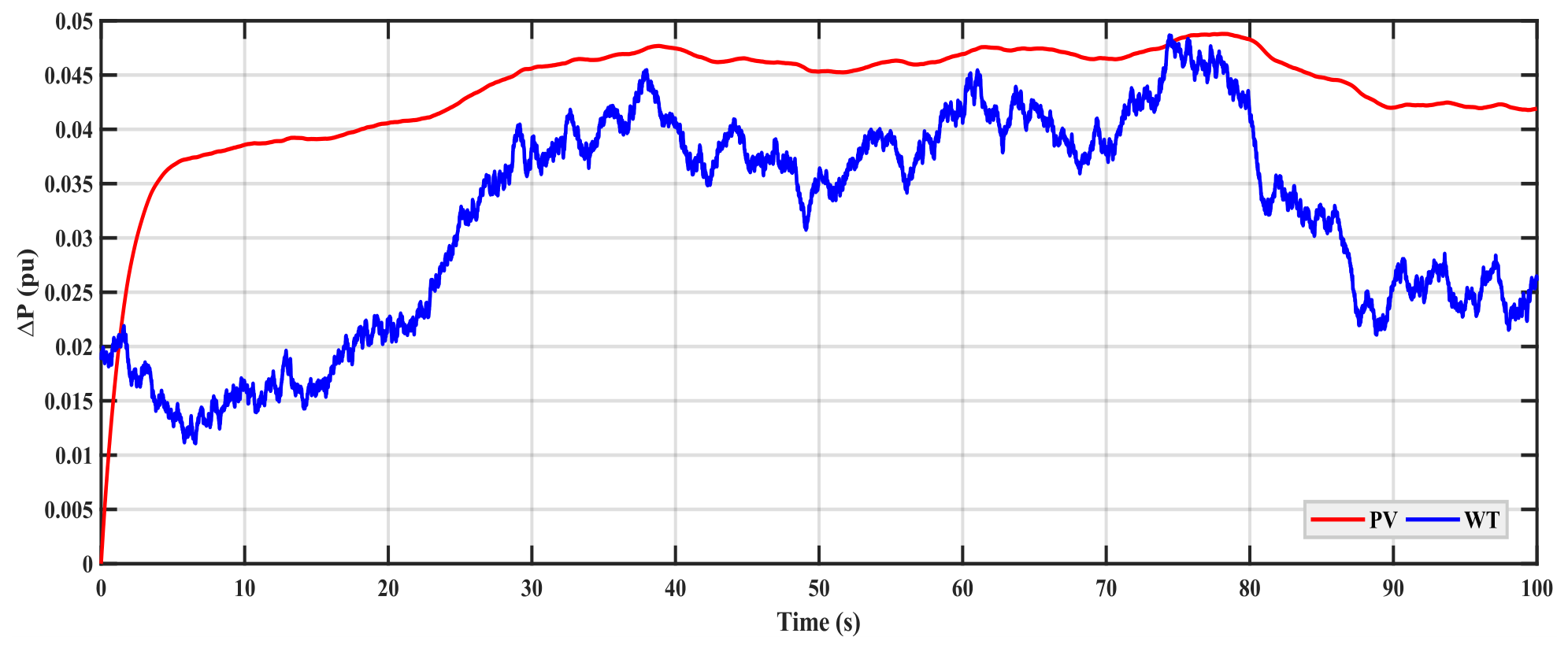
5.5. Case 2—Scenario 2: Fixed Load Increase Under Random RES Profiles

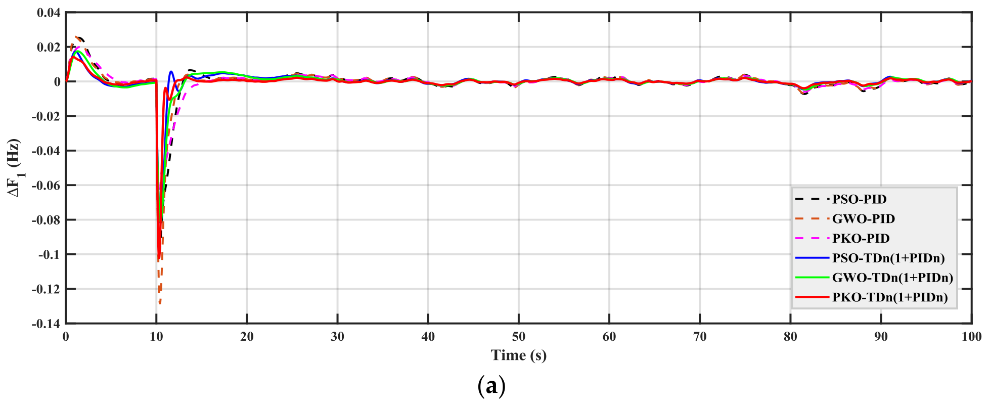
This scenario uses the same disturbance (a +0.1 pu Δ P D in area 1 at t = 10 s) but replaces the uniform RES profiles with random PV and WT profiles in areas 1 and 2, respectively. The resulting dynamic responses, including F 1 , F 2 , and P t i e , are recorded for system performance assessment under random RES variability. Figure 20 illustrates the random solar and wind power injected into the PS.
Based on Figure 21 and Table 14 and Table 15, the results confirm that the PKO-TDn(1+PIDn) controller delivers the best overall transient performance. For F 1 , it reduces undershoot by 20.3% compared with GWO-TDn(1+PIDn) and by 15.4% compared with PSO-TDn(1+PIDn) while improving over the PID-based controllers by 20–28%. Its overshoot is also smaller, decreasing by 16.4% relative to GWO-TDn(1+PIDn), by 18.8% relative to PSO-TDn(1+PIDn), and by 43–77% compared with the PID group. For F 2 , PKO-TDn(1+PIDn) reduces undershoot by 42.8% vs. GWO-TDn(1+PIDn) and by 9% vs. PSO-TDn(1+PIDn), with an additional 12–43% improvement over the PID-based schemes.
The overshoot improvement in F 2 follows the same pattern, with reductions of 5–16% over the TDn(1+PIDn)-based ones and 44–78% over the PID-based ones. P t i e also shows clear gains; undershoot decreases by 12.1% compared with GWO-TDn(1+PIDn), by 23.1% compared with PSO-TDn(1+PIDn), and by 21–30% relative to the PID group, while overshoot is reduced by 26–35% vs. the TDn(1+PIDn)-based methods and 53–76% vs. PID. Overall, PKO-TDn(1+PIDn) provides the strongest damping and the smallest transient deviations in scenario 2.

5.6. Case 2—Scenario 3: Random Load Change Under Uniform RES Profiles

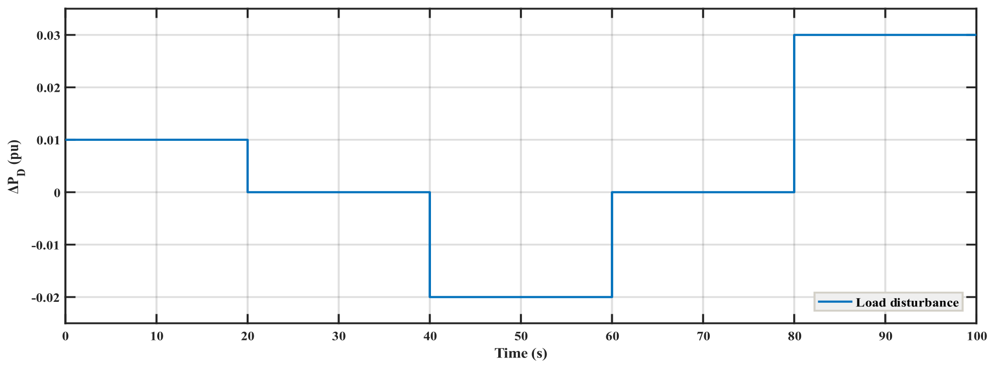
In this scenario, the load in area 1 is subjected to a randomly varying disturbance Δ P D . The PV and WT power profiles follow the same uniform pattern used in scenario 1. The corresponding system responses, F 1 , F 2 , and P t i e , are recorded to evaluate system behavior under random loading conditions and uniform RES profiles. Figure 22 shows the random load change subjected to the PS.
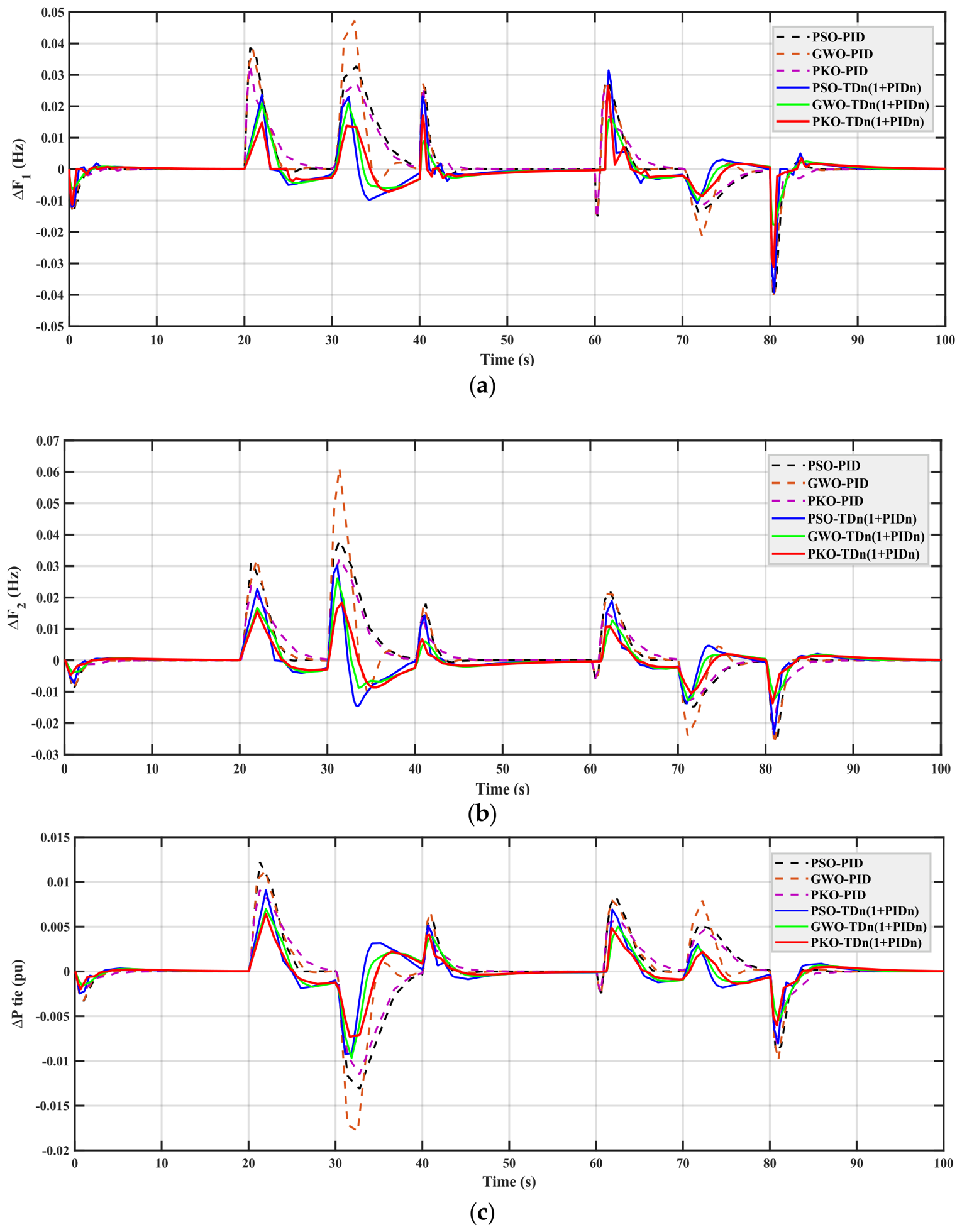
Based on Figure 18 and Figure 23, and Table 14 and Table 15, it is evident that the TDn(1+PIDn) controller clearly outperforms all PID-based methods. The GWO-TDn(1+PIDn) controller achieves the smallest undershoot in F 1 and F 2 , reducing the F 1 undershoot by 43% and the F 2 undershoot by 6% compared with the next-best controller. The PKO-TDn(1+PIDn) method provides the lowest overshoot in both areas, lowering the F 2 overshoot by 30% relative to GWO-TDn(1+PIDn). For P t i e , PKO-TDn(1+PIDn) again gives the best result, reducing undershoot by 21% and overshoot by 8%. Overall, the TDn(1+PIDn) family provides substantial percentage improvements in damping and stability, confirming its superiority under the most severe conditions.

5.7. Case 2—Scenario 4: Random Load Change Under Random RES Profiles

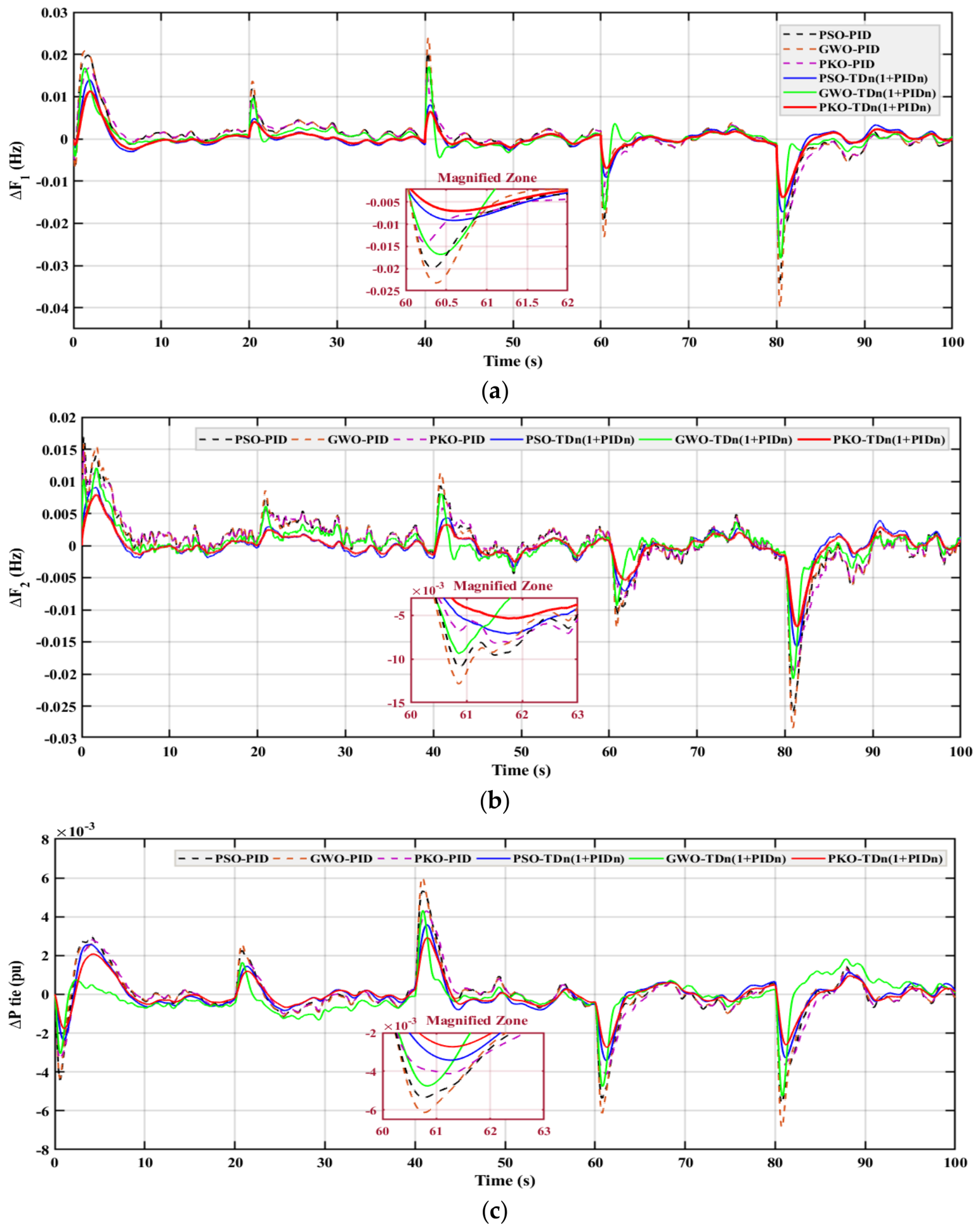
In this scenario, a random load disturbance Δ P D is applied in area 1 at t = 10 s, following the same loading pattern as in scenario 3. The PV and WT power profiles follow the same random pattern used in scenario 2. The system responses F 1 , F 2 , and P t i e , are recorded to evaluate system behavior under random loading conditions and random RES variability.
Based on Figure 20, Figure 22 and Figure 24 and Table 14 and Table 15, it is evident that the PKO-TDn(1+PIDn) delivers the best performance among all methods. For F 1 , it reduces undershoot by 19.7% and overshoot by 34.0% relative to the next-best TDn(1+PIDn) controller. In F 2 , it again shows the smallest deviations, improving undershoot by 19.8% and overshoot by 34.4%. For P t i e , PKO-TDn(1+PIDn) reduces undershoot by 22.7% and overshoot by 32.3% compared with the next-best TDn(1+PIDn) design. Overall, the PKO-TDn(1+PIDn) method provides consistent and significant improvements of 20–34% across all transient indices.

5.8. Case 3—Scenario 1: Fixed Load Increase Under Uniform RES Profiles with ESSs

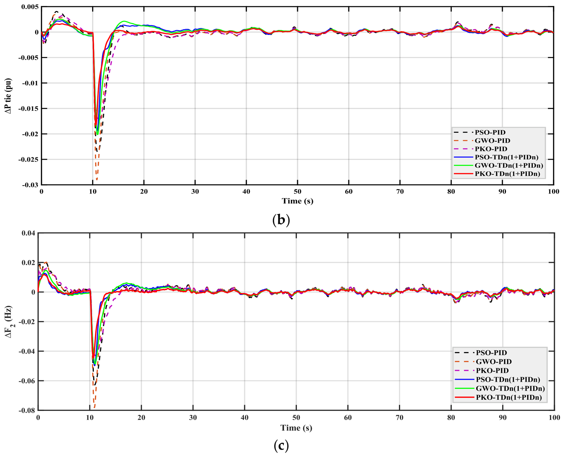
This scenario uses the same disturbance (a +0.1 pu Δ P D in area 1 at t = 10 s), and the PV and WT injections follow uniform profiles, matching the loading and RES conditions previously considered in case 2 scenario 1.
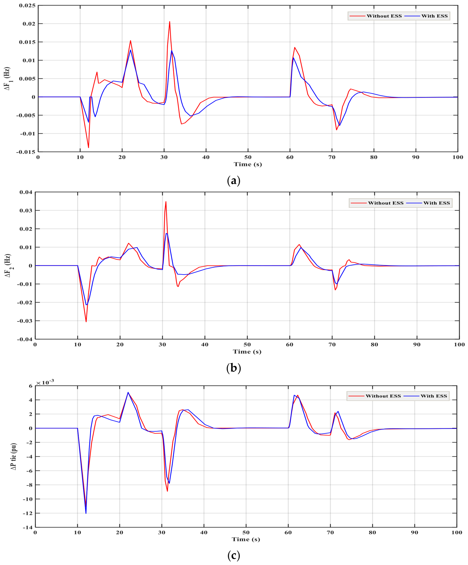
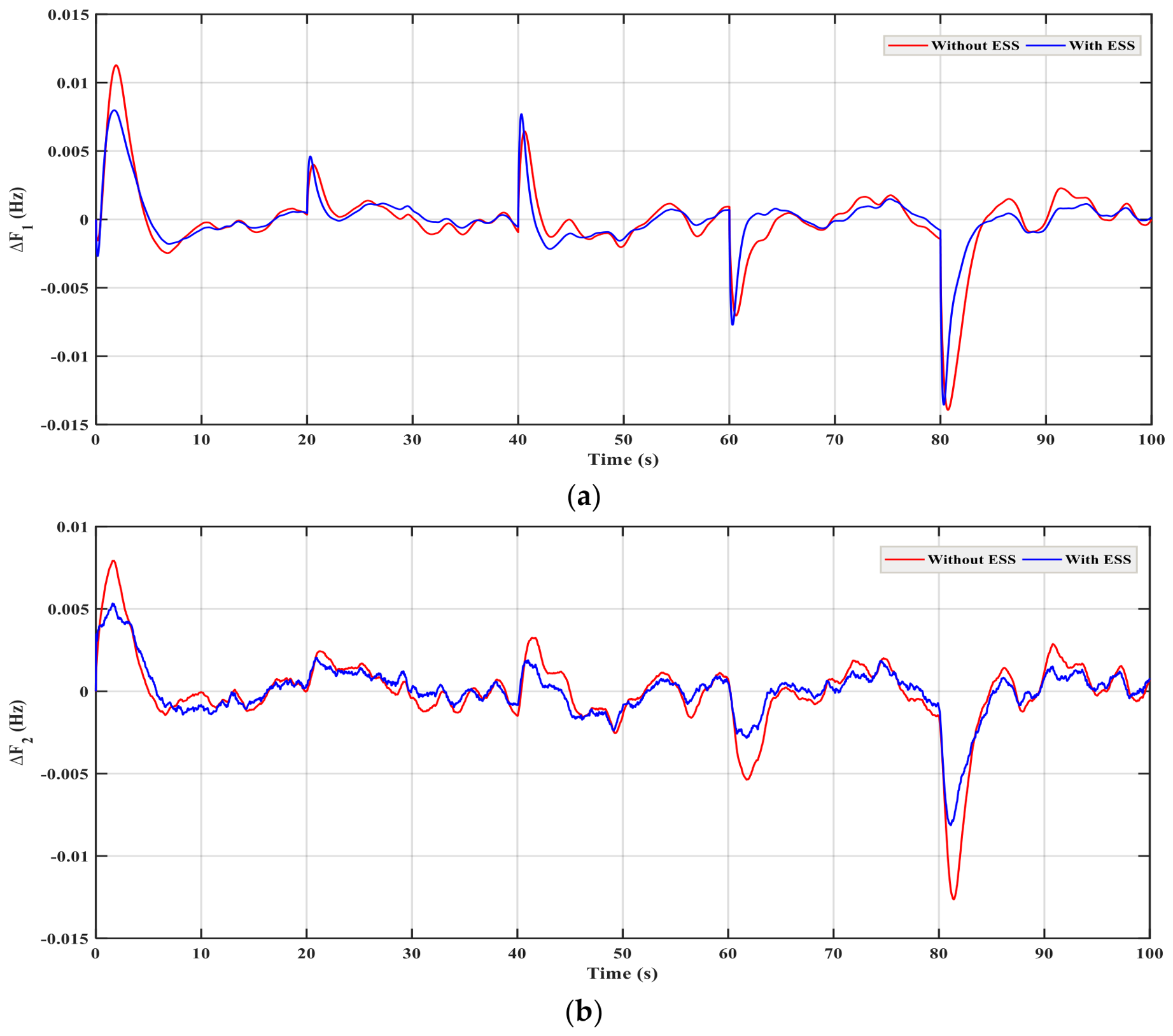
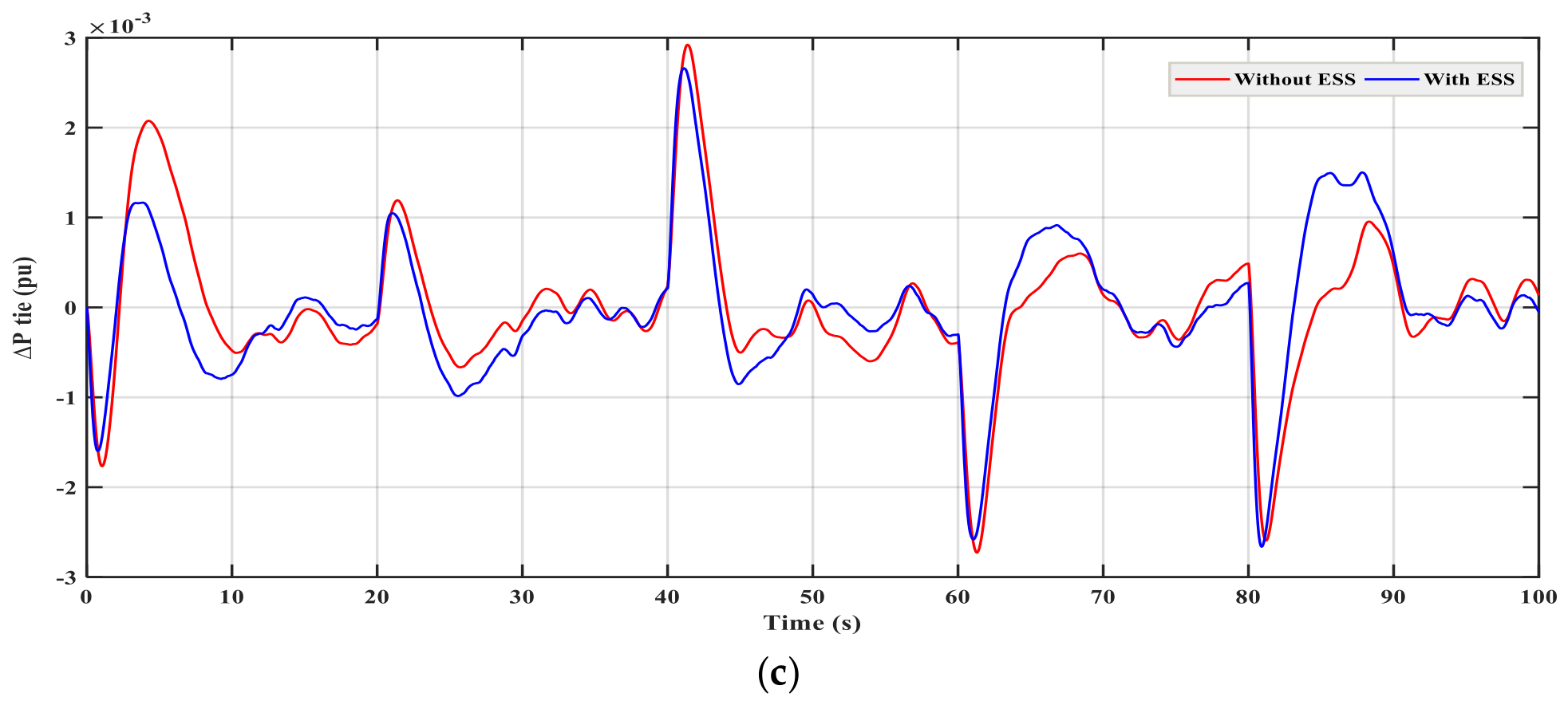
ESSs are incorporated into the system to enhance frequency support during the disturbance. Area 1 is supported by VRFB and SMES, while area 2 is supported by VRFB and HAFC. The resulting dynamic responses, including F 1 , F 2 , and P t i e , are recorded for system performance assessment and for studying the impact of ESS integration under uniform RES profiles, and the results are compared with the RES-only case. According to Figure 25 and Table 16 and Table 17, it is shown that with ESS support, the PKO-TDn(1+PIDn) controller shows major improvements in scenario 1. F 1 improves by 44% in undershoot and 50% in overshoot, and F 2 improves by 30% in undershoot and 50% in overshoot.
P t i e undershoots improve moderately by 14%, while P t i e overshoot increases slightly by 1.4%. The ITAE value also decreases, confirming faster settling and better damping. Overall, ESSs significantly enhance frequency stability by lowering oscillations by 30–50%. They also support better tie-line behavior, helping the system recover faster and reducing power swings between the areas.

5.9. Case 3—Scenario 2: Fixed Load Increase Under Random RES Profiles with ESSs

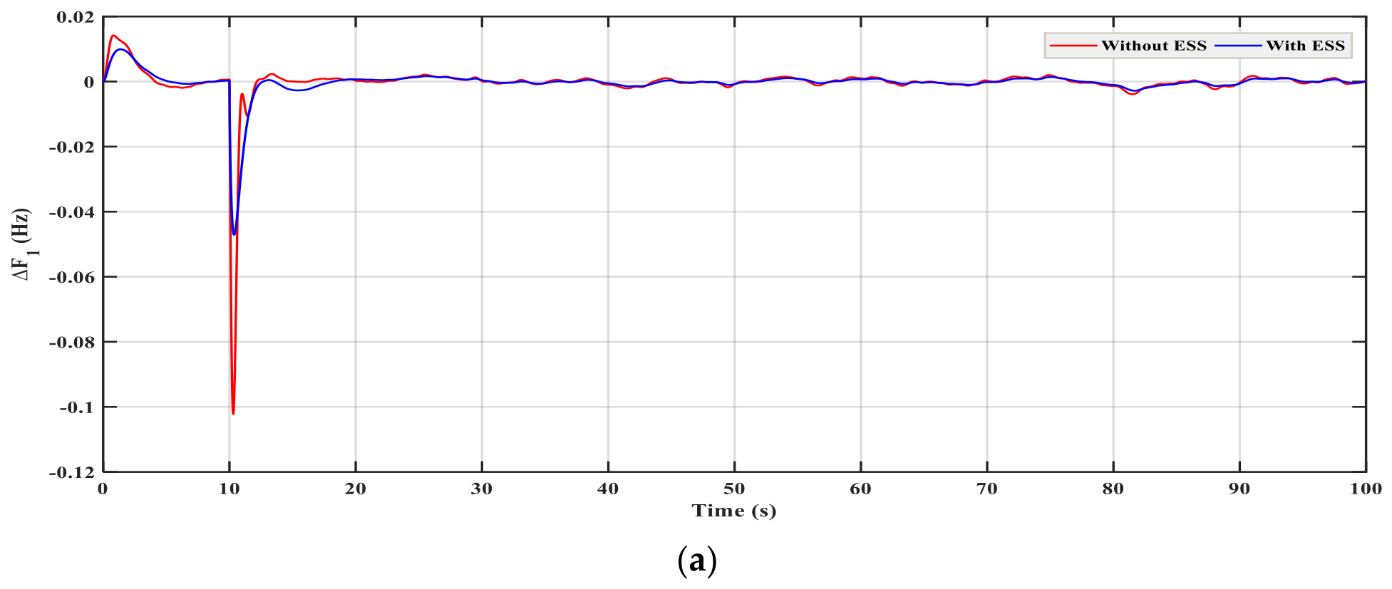
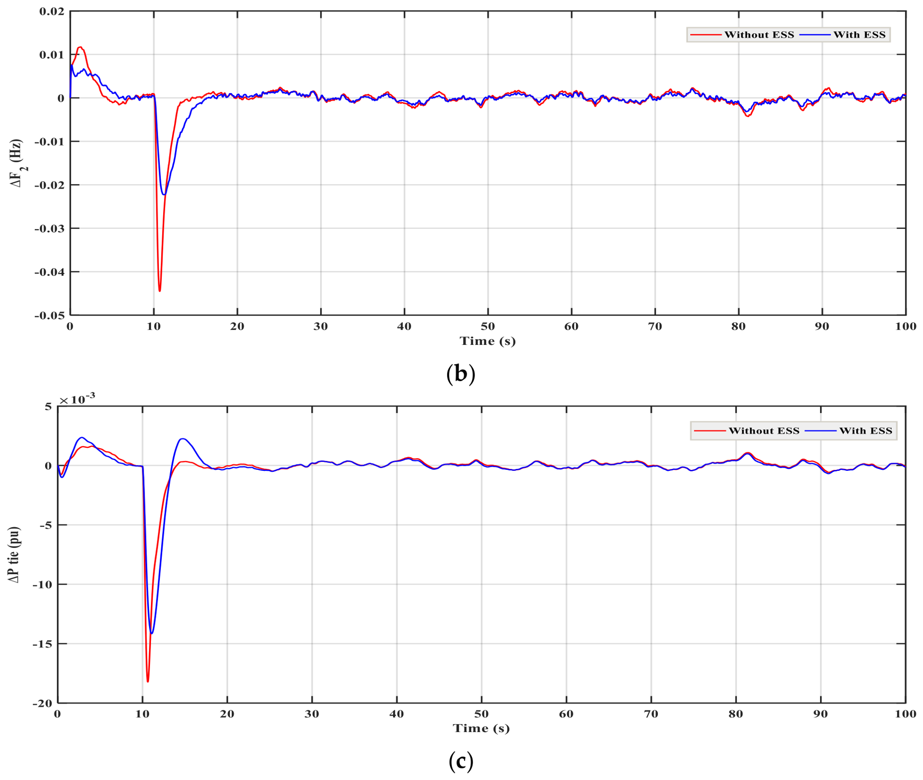
This scenario uses the same disturbance (a +0.1 pu Δ P D in area 1 at t = 10 s), and the PV and WT injections follow random profiles, matching the loading and RES conditions previously considered in case 2 scenario 2. ESSs are added to the system to enhance frequency stability and support RESs during the disturbance. Similar to scenario 1, area 1 incorporates VRFB and SMES, and area 2 incorporates VRFB and HAFC. The resulting responses ( F 1 , F 2 , P t i e ) are compared with the RES-only case to study the ESS impact.
It is noticeable from Figure 26 and Table 18 and Table 19 that, in scenario 2, adding ESSs helps the system recover more smoothly from disturbances.
Frequency deviations in both areas drop sharply, with undershoot reduced by about 50% and overshoot lowered by 30–35%. The tie-line response also becomes more stable; undershoots improve by 22%, and overshoot decreases dramatically by 85%. Overall, ESSs make the system more stable, less oscillatory, and faster in returning to normal conditions.

5.10. Case 3—Scenario 3: Random Load Change Under Uniform RES Profiles with ESSs

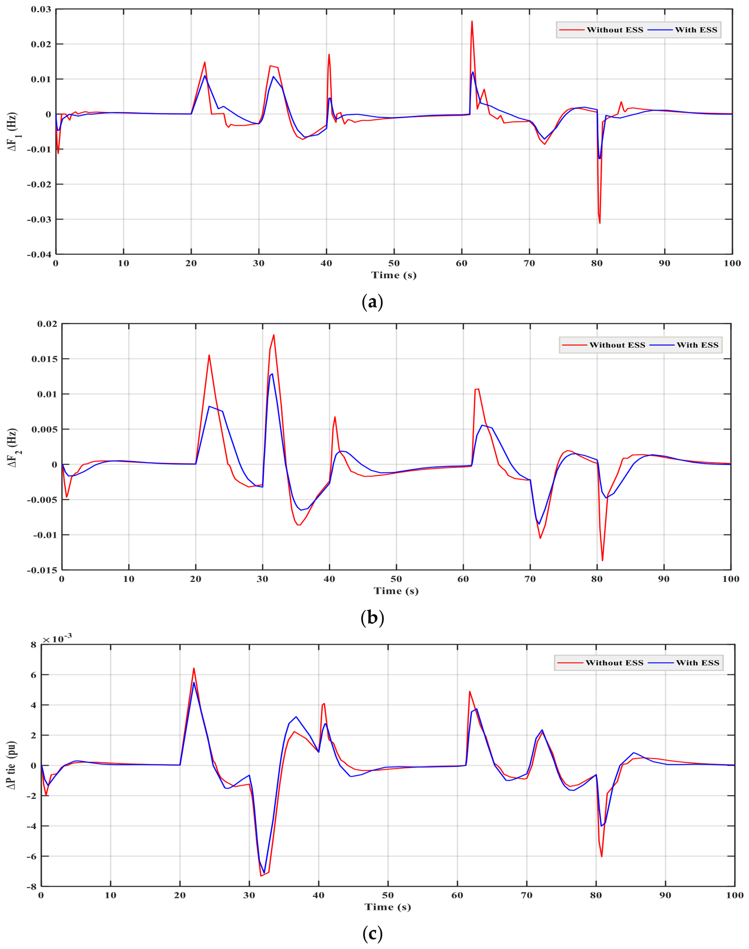
This scenario uses the same random load disturbance, and the PV and WT injections follow uniform profiles, matching the loading and RES conditions previously considered in case 2 scenario 3. Both areas use the same ESS arrangement. The system responses ( F 1 , F 2 , P t i e ) are compared with the RES-only case to study the ESS impact in this scenario.
Based on Figure 27 and Table 20 and Table 21, it is evident that with ESSs, the system performance in scenario 3 improves notably. Frequency deviations in area 1 show the strongest gains, with 59–61% reductions in undershoot and overshoot. Area 2 also improves, with 30–35% lower deviation magnitudes. Tie-line oscillations decrease as well, with 3% better undershoot and 15% better overshoot. Overall, ESSs make the system more stable, less oscillatory, and quicker to settle.

5.11. Case 3—Scenario 4: Random Load Change Under Random RES Profiles with ESSs

This scenario uses the same random load disturbance, and the same PV and WT random profiles, matching the loading and RES conditions previously considered in case 2 scenario 4. Both areas use the same ESS arrangement.
The resulting dynamic responses, including F 1 , F 2 , and P t i e are recorded for system performance assessment and for studying the impact of ESS integration under random loading conditions and random RES profiles, and the results are compared with the RES-only case for the same conditions and system parameters.
Based on Figure 28 and Table 22 and Table 23, it is evident that, in scenario 4, adding ESSs leads to consistent performance improvements across the system. F 1 undershoot improves by 3% and overshoot by 29%, while F 2 shows stronger gains, with undershoot reduced by 36% and overshoot by 33%. P t i e also benefits, with 2% improvement in undershoot and 9% in overshoot. Importantly, the overall ITAE drops from 16.5372 to 12.3843, representing a 25% reduction, confirming that ESSs enhance damping, speed up recovery, and reduce the cumulative error over time in system performance.
Beyond the dynamic contribution quantified above, the three ESSs differ markedly once cost, service life, energy and power density and siting are taken into account, and these differences shape where each is most sensibly deployed. The SMES offers very high power density and a near-instantaneous response, which suits short, high-power support, though at a high capital cost per unit of stored energy and with the standing burden of cryogenic cooling. The VRFB combines high energy density with a long cycle life and a comparatively efficient round trip, which suits the smoothing of sustained renewable swings, though the electrolyte tank volume needed for large-scale deployment remains a siting consideration. The HAFC sits between these roles, offering long-duration balancing through the hydrogen path, but with a round-trip efficiency of only about 20–40% and a durability that is sensitive to frequent load cycling. Read together, these characteristics suggest a complementary rather than competing role for the three technologies in area 1 (VRFB and SMES) and area 2 (VRFB and HAFC), consistent with the combined improvement reported for the ESS-assisted scenarios above. The previous simulations quantify the combined effect of the paired devices in each area rather than isolating each device’s individual contribution.

5.12. Case 4: Validation by OPAL-RT Simulator

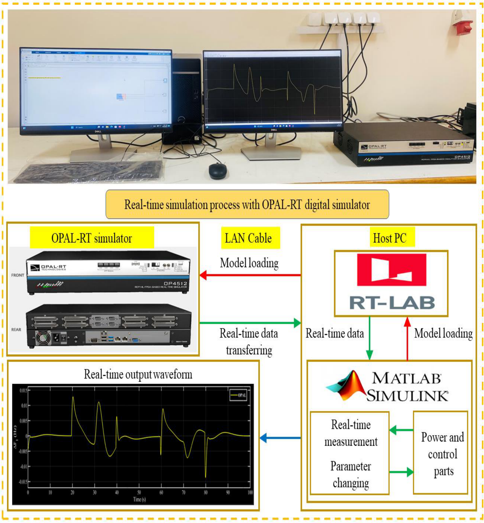
The OPAL-RT simulator is employed to experimentally verify the real-time behavior of the proposed PKO-TDn(1+PIDn) method. Instead of relying solely on offline simulations, MATLAB/Simulink models are deployed to the OPAL-RT simulator to enable hardware-in-the-loop (HIL) execution, ensuring that the controller is assessed under realistic computational conditions in which numerical delays, communication latencies, and execution imperfections naturally occur that are not captured in conventional offline simulations [77,78]. The HIL configuration is composed of several coordinated components that work together to create a realistic real-time testing environment. At the center of this setup is a high-performance host PC with an Intel Core i7-10700 CPU processor, which serves as the command and compilation station that compiles the MATLAB/Simulink models using RT-LAB and an OP4512 real-time simulator that executes the power–system dynamics. When transferring the model from offline simulation to the real-time simulator, the model was discretized using a fixed-step ode4 (Runge–Kutta) solver at a step size of 10 µs, selected to meet the real-time deadline of the OP4512 while preserving the dynamics of interest.
The model is split into a Master subsystem (SM), which runs the plant and controllers in real time under a hard 10 μs frame, and a console subsystem (SC) on the host, which passively monitors F 1 , F 2 , and P t i e via the OpComm blocks that handle real-time data exchange over the high-speed link between the target and the host, ensuring the captured signals genuinely reflected what the target computed, without any alteration. The only change needed for real-time deployment was replacing the offline variable-step solver with a fixed-step solver at a step size, chosen to meet the timing deadline while still capturing the relevant transient dynamics; controller gains and system parameters are left unchanged. The resulting real-time traces closely matched the offline results in undershoot, overshoot, and settling time, with no execution overruns, and stable closed-loop behavior throughout.
Both units are linked through a high-speed network to enable continuous data exchange and synchronized operation. This setup provides a reliable platform for evaluating the real-time performance and robustness of the proposed control strategy.
This arrangement ensures that the controller is tested under realistic conditions, including computation delays, task-scheduling constraints, and numerical discretization effects, thereby allowing for a more reliable assessment of its real-time operability and robustness. Figure 29 illustrates the OPAL-RT experimental setup.
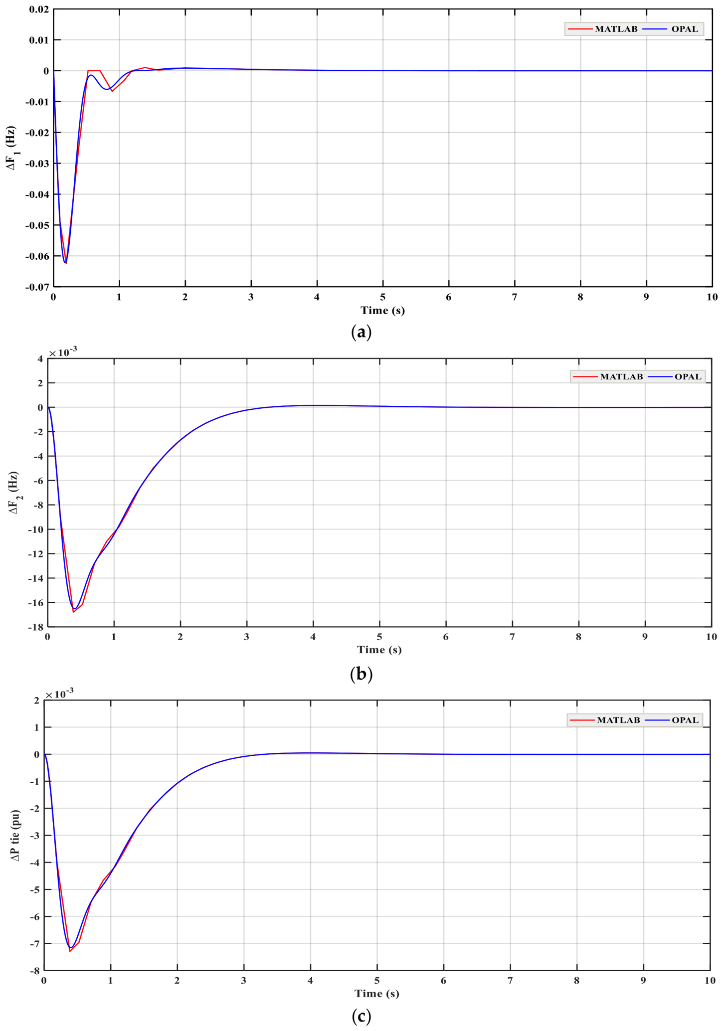
The OPAL-RT simulation and MATLAB simulation results are compared for case 1 scenario 1 in Figure 30, case 2 scenario 1 in Figure 31, and case 3 scenario 3 in Figure 32. From the figures, the MATLAB results are approximately similar to the OPAL-RT simulation results, demonstrating that the proposed approach maintains its effectiveness when executed on real-time hardware. The consistency between the offline MATLAB simulation and the OPAL-RT real-time implementation was quantitatively evaluated using the maximum absolute error, root mean square error (RMSE), and normalized root mean square error (NRMSE), as presented in Table 24.
The obtained results demonstrate a high level of agreement between both simulators for all investigated scenarios. For the deviations including F 1 , F 2 , and P t i e , the maximum absolute errors remain within acceptable limits, confirming that the discretized real-time model preserves the dynamic behavior of the original offline model.
For the C1–S1 operating condition, the NRMSE values are limited to 1.4%, 1.1%, and 1.1% for F 1 , F 2 , and P t i e , respectively, indicating excellent matching between MATLAB and OPAL-RT results. Under more severe operating scenarios (C2–S1 and C3–S3), the highest observed NRMSE remains below 13.24%, while most signals maintain errors below 7%. These deviations are mainly attributed to the fixed-step discretization and real-time execution constraints of the OPAL-RT simulator.
The small differences between offline and real-time responses confirm the feasibility of implementing the proposed controller in a real-time environment. As the realized controller is a fixed low-order linear structure, its online computational burden is negligible, and no execution overruns or instabilities occurred during operation.
Therefore, the OPAL-RT results validate not only the dynamic performance of the proposed PKO-TDn(1+PIDn) method but also its practical applicability for hardware-in-the-loop testing.

6. Conclusions

In this study, the LFC was investigated for a two-area interconnected PS comprising non-reheat thermal plants. The capability of the proposed control scheme to handle a nonlinear multi-area system with different control parameters for each area was demonstrated by studying the test system while considering nonlinearity sources such as GRC, GDB, and CTD. By integrating a multi-stage TDn(1+PIDn) controller with PKO and ITAE serving as the OF, dynamic challenges such as frequency deviations and tie-line power fluctuations were reduced. The PKO-TDn(1+PIDn) method was compared in detail to a number of other methods, such as GWO-TDn(1+PIDn), PSO-TDn(1+PIDn), PKO-PID, GWO-PID, and PSO-PID. The inclusion of PV in area 1 and WT in area 2 intensifies the fluctuations within the system. System performance was assessed under a range of operating conditions, such as step and random load changes, and uniform and random RES power profiles. ESSs were added, VRFB and SMES in area 1, alongside VRFB and HAFC in area 2, to mitigate RES variability by absorbing surplus energy and rapidly injecting power during deficits, thereby reducing overshoot, undershoot, and settling time across all tested scenarios. The proposed PKO-TDn(1+PIDn) method outperformed the other methods and consistently delivered superior damping characteristics across these diverse operating conditions. The HIL experiments on the OPAL-RT OP4512 simulator validated the proposed controller’s practical applicability, showing strong agreement with offline simulations with no overruns or instability, which confirmed reliable implementation on FPGA-based real-time hardware. In short, the tilt-derivative and filtered-PID stages tuned by PKO accounted for the improved transient indices, while the layered ESS support suppressed the frequency and tie-line deviations introduced by solar and wind intermittency.
Future work may include:
  • Extending the approach to larger multi-area and inverter-dominated microgrids, including coordinated grid-forming inverter control, where advanced robust strategies such as sliding-mode control have proven effective [79].
  • Modeling the long-term degradation and lifetime economics of the storage units, the HAFC in particular, under frequent LFC service, drawing on evidence of PEMFC health sensitivity to operating temperature and durability-enhancing strategies [80].
  • Evaluating different energy storage technologies, such as pumped hydro storage, supercapacitors, flywheels and hybrid systems, within the same control framework.
  • Studying the impact of EV integration and FACTS devices on tie-line power control and overall stability.

Author Contributions

Conceptualization, H.S.E.M. and H.M.H.F.; methodology, H.M.A., S.A.A. and M.N.A.-W.; software, H.M.A.; validation A.-W.I., and A.M.A.-S.; formal analysis, S.A.A. and A.-W.I.; data curation, M.N.A.-W.; writing—original draft preparation, H.M.A., H.S.E.M. and S.A.A.; writing—review and editing, H.M.H.F., M.N.A.-W. and A.M.A.-S.; visualization, M.N.A.-W. and S.A.A.; supervision, H.S.E.M.; project administration, H.M.H.F.; funding acquisition, A.M.A.-S. All authors have read and agreed to the published version of the manuscript.

Funding

This work was supported by the Ongoing Researchers Funding Program, King Saud University, Riyadh, Saudi Arabia, under grant ORF-2026-337.

Data Availability Statement

The data that support the findings of this study are available from the corresponding authors upon reasonable request.

Conflicts of Interest

I, as the corresponding author, hereby declare on behalf of all the authors that we do not have any genuine or potential conflicts of interest. This includes but is not limited to financial, personal, or other relationships such as employment, consultancy, stock ownership, honoraria, paid expert testimony, patent applications/registrations, and grants or other funding from individuals or organizations of the work submitted. We affirm that these factors have not and will not inappropriately influence our work.

Abbreviations

The following abbreviations are used in this manuscript:
LFCLoad frequency control
RESsRenewable energy sources
ESSsEnergy storage systems
HILHardware-in-the-loop
ITAEIntegral of time-weighted absolute error
PSOParticle swarm optimization
GWOGrey wolf optimization
PKOPied kingfisher optimizer
PIDProportional integral derivative
TDn(1+PIDn)Tilted derivative of order n combined with a proportional–integral–derivative controller with n-th order derivative
HAFCHydrogen aqua electrolyzer fuel cell
SMESSuper magnetic energy storage
VRFBVanadium redox flow battery
WTWind turbine
PVPhotovoltaic system
PSPower system
GRCGeneration rate constraint
GDBGovernor dead band
CTDCommunication time delay
MPCModel predictive control
AIArtificial intelligence
RCARobust control approaches
FLCFuzzy logic control
RSORat swarm optimization
CGOChaos game optimization
WHOWild horse optimizer
EOAEquilibrium optimization algorithm
WOAWalrus optimization algorithm
HBAHoney badger algorithm
SSASalp swarm algorithm
MOMSAMulti-objective mantis search algorithm
GJOGolden jackal optimization
BDGOABio-dynamic grasshopper optimization algorithm
DCSADiligent crow search algorithm
BOABrown bear optimization algorithm
ZOAZebra optimization algorithm
QORSAQuasi-opposition reptile search algorithm
EVElectric vehicle
HVDCHigh voltage direct current
COAChimp optimization algorithm
GTOGorilla troops optimizer
GSAGravitational search algorithm
BABat algorithm
ADIWACOAdaptive dynamic inertia weight acceleration coefficient optimization
FESSFlywheel energy storage system
BESSBattery energy storage system
UCUltracapacitor
MOAMother optimization algorithm
CESCapacitor energy storage
NRELNational renewable energy laboratory
EPSDEEnsemble of parameters and strategies differential evolution
CLPSOComprehensive learning particle swarm optimization
HPSO-PSHybrid particle swarm optimization and pattern search
OFObjective function
RMSERoot mean square error
NRMSENormalized root mean square error
Indices
RSpeed regulation (Hz/pu MW)
ΔFFrequency deviation (Hz)
ΔPtieChange in tie-line power (pu)
ΔPDChange in load power (pu)
T12Tie-line synchronizing coefficient
BFrequency bias parameter (pu MW/Hz)
DLoad frequency dependency parameter (MW/Hz)
HInertia constant of the generator (s)
PDNominal load (MW)
FNominal frequency (Hz)
τCommunication time delay (s)
ACEArea control error
KGGenerator gain constant
KTTurbine gain constant
KPPower system gain constant
KPVPhotovoltaic system gain constant
KWTWind system gain constant
TGGenerator time constant (s)
TTTurbine time constant (s)
TPPower system time constant (s)
TPVPhotovoltaic system time constant (s)
TWTWind system time constant (s)
USUndershoot
OSOvershoot
TsSettling time (s)
KD, KDD, KP, KIDerivative, proportional and integral gains of controller
N, NN, nController filters
PwindWind turbine power (MW)
λTTip speed ratio
λ1Effective tip speed ratio
ATSwept area of the turbine (m2)
ωrRotor speed (rpm)
CPTurbine performance coefficient
VWind speed (m/s)
ρAir density (Kg/m3)
VTPTip speed (m/s)
βBlade pitch angle (°)
RBlade radius (m)
KaeAqua electrolyzer gain constant
KfcFuel cell gain constant
TaeAqua electrolyzer time constant (s)
TfcFuel cell time constant (s)
T1, T2, T3, T4Lead-lag blocks time constant (s)
KSMESSuper magnetic energy storage gain constant
TSMESSuper magnetic energy storage time constant (s)
KRFBVanadium redox flow battery gain constant
TcRFBResetting vanadium redox flow battery time constant (s)
TdRFBVanadium redox flow battery time delay constant (s)
ΔPsolarVariance in PV output power (pu)
KnConversion factor
P H 2 Power output from the hydrogen fuel cell (MW)
PWTPower generated from WT (MW)
PPVPower generated from PV (MW)

References

  1. Ranjan, M.; Shankar, R. A literature survey on load frequency control considering renewable energy integration in power system: Recent trends and future prospects. J. Energy Storage 2022, 45, 103717. [Google Scholar] [CrossRef]
  2. Gulzar, M.M.; Iqbal, M.; Shahzad, S.; Muqeet, H.A.; Shahzad, M.; Hussain, M.M. Load frequency control (LFC) strategies in renewable energy-based hybrid power systems: A review. Energies 2022, 15, 3488. [Google Scholar] [CrossRef]
  3. Arya, Y. Automatic generation control of two-area electrical power systems via optimal fuzzy classical controller. J. Frankl. Inst. 2018, 355, 2662–2688. [Google Scholar] [CrossRef]
  4. Sattar, F.; Ghosh, S.; Isbeih, Y.J.; El Moursi, M.S.; Al Durra, A.; El Fouly, T.H.M. A predictive tool for power system operators to ensure frequency stability for power grids with renewable energy integration. Appl. Energy 2024, 353, 122226. [Google Scholar] [CrossRef]
  5. Sun, B.; Zhang, Z.; Hu, J.; Meng, Z.; Huang, B.; Li, N. An energy storage capacity configuration method for a provincial power system considering flexible adjustment of the tie-line. Energies 2024, 17, 270. [Google Scholar] [CrossRef]
  6. Gulzar, M.M.; Sibtain, D.; Alqahtani, M.; Alismail, F.; Khalid, M. Load frequency control progress: A comprehensive review on recent development and challenges of modern power systems. Energy Strategy Rev. 2025, 57, 101604. [Google Scholar] [CrossRef]
  7. Masikana, S.B.; Sharma, G.; Sharma, S. Renewable energy sources integrated load frequency control of power system: A review. E-Prime-Adv. Electr. Eng. Electron. Energy 2024, 8, 100605. [Google Scholar] [CrossRef]
  8. El-Hameed, M.A.; Saeed, M.; Kabbani, A.; Abd El-Hay, E. Efficient load frequency controller for a power system comprising renewable resources based on deep reinforcement learning. Sci. Rep. 2025, 15, 18379. [Google Scholar] [CrossRef] [PubMed]
  9. Li, Z.; Deusen, D. Role of energy storage technologies in enhancing grid stability and reducing fossil fuel dependency. Int. J. Hydrogen Energy 2025, 102, 1055–1074. [Google Scholar] [CrossRef]
  10. Khamies, M.; Magdy, G.; Kamel, S.; Khan, B. Optimal model predictive and linear quadratic gaussian control for frequency stability of power systems considering wind energy. IEEE Access 2021, 9, 116453–116474. [Google Scholar] [CrossRef]
  11. Magdy, G.; Shabib, G.; Elbaset, A.A.; Mitani, Y. Optimized coordinated control of LFC and SMES to enhance frequency stability of a real multi-source power system considering high renewable energy penetration. Prot. Control Mod. Power Syst. 2018, 3, 39. [Google Scholar] [CrossRef]
  12. Ramesh, M.; Yadav, A.K.; Pathak, P.K. Artificial gorilla troops optimizer for frequency regulation of wind contributed microgrid system. J. Comput. Nonlinear Dyn. 2023, 18, 011005. [Google Scholar]
  13. Jagatheesan, K.; Anand, B.; Dey, N.; Ashour, A.S.; Balas, V.E. Load frequency control of hydro-hydro system with fuzzy logic controller considering non-linearity. In Recent Developments and the New Direction in Soft-Computing Foundations and Applications: Selected Papers from the 6th World Conference on Soft Computing, May 22–25, 2016, Berkeley, USA; Springer: Berlin/Heidelberg, Germany, 2018; pp. 307–318. [Google Scholar]
  14. Sah, S.V.; Prakash, V.; Pathak, P.K.; Yadav, A.K. Fractional order AGC design for power systems via artificial gorilla troops optimizer. In 2022 IEEE International Conference on Power Electronics, Drives and Energy Systems (PEDES); IEEE: New York, NY, USA, 2022; pp. 1–6. [Google Scholar]
  15. Sharma, M.; Dhundhara, S.; Arya, Y.; Prakash, S. Frequency excursion mitigation strategy using a novel COA optimised fuzzy controller in wind integrated power systems. IET Renew. Power Gener. 2020, 14, 4071–4085. [Google Scholar] [CrossRef]
  16. Tasnin, W.; Saikia, L.C. Deregulated AGC of multi-area system incorporating dish-Stirling solar thermal and geothermal power plants using fractional order cascade controller. Int. J. Electr. Power Energy Syst. 2018, 101, 60–74. [Google Scholar] [CrossRef]
  17. Nandi, M.; Shiva, C.K.; Mukherjee, V. Moth-flame algorithm for TCSC-and SMES-based controller design in automatic generation control of a two-area multi-unit hydro-power system. Iran. J. Sci. Technol. Trans. Electr. Eng. 2020, 44, 1173–1196. [Google Scholar]
  18. Jagatheesan, K.; Anand, B.; Dey, N.; Ashour, A.S.; Balas, V.E. Load frequency control of multi-area interconnected thermal power system: Artificial intelligence-based approach. Int. J. Autom. Control 2018, 12, 126–152. [Google Scholar] [CrossRef]
  19. Eltamaly, A.M.; Zaki Diab, A.A.; Abo-Khalil, A.G. Robust control based on H∞ and linear quadratic gaussian of load frequency control of power systems integrated with wind energy system. In Control and Operation of Grid-Connected Wind Energy Systems; Springer: Berlin/Heidelberg, Germany, 2021; pp. 73–86. [Google Scholar]
  20. Yakout, A.H.; Kotb, H.; Hasanien, H.M.; Aboras, K.M. Optimal fuzzy PIDF load frequency controller for hybrid microgrid system using marine predator algorithm. IEEE Access 2021, 9, 54220–54232. [Google Scholar] [CrossRef]
  21. Danaeefar, H.; Barati, H.; Shirmardi, S.A. Optimal control of PID-FUZZY based on gravitational search algorithm for load frequency control. Int. J. Eng. Res. 2019, 8, IJERTV8IS050013. [Google Scholar] [CrossRef]
  22. Sharma, J.; Hote, Y.V.; Prasad, R. Robust PID load frequency controller design with specific gain and phase margin for multi-area power systems. IFAC-PapersOnLine 2018, 51, 627–632. [Google Scholar] [CrossRef]
  23. Magdy, G.; Mohamed, E.A.; Shabib, G.; Elbaset, A.A.; Mitani, Y. SMES based a new PID controller for frequency stability of a real hybrid power system considering high wind power penetration. IET Renew. Power Gener. 2018, 12, 1304–1313. [Google Scholar] [CrossRef]
  24. Sekyere, Y.O.M.; Effah, F.B.; Okyere, P.Y. Optimal tuning of PID controllers for LFC in renewable energy source integrated power systems using an improved PSO. J. Electron. Electr. Eng. 2024, 3, 68–87. [Google Scholar]
  25. Gopi, P.; Alluraiah, N.C.; Kumar, P.H.; Bajaj, M.; Blazek, V.; Prokop, L. Improving load frequency controller tuning with rat swarm optimization and porpoising feature detection for enhanced power system stability. Sci. Rep. 2024, 14, 15209. [Google Scholar] [CrossRef] [PubMed]
  26. Ali, G.; Aly, H.; Little, T. Automatic generation control of a multi-area hybrid renewable energy system using a proposed novel GA-fuzzy logic self-tuning PID controller. Energies 2024, 17, 2000. [Google Scholar] [CrossRef]
  27. Barakat, M. Novel chaos game optimization tuned-fractional-order PID fractional-order PI controller for load-frequency control of interconnected power systems. Prot. Control Mod. Power Syst. 2022, 7, 16. [Google Scholar] [CrossRef]
  28. Çelik, E.; Öztürk, N.; Arya, Y.; Ocak, C. (1 + PD)-PID cascade controller design for performance betterment of load frequency control in diverse electric power systems. Neural Comput. Appl. 2021, 33, 15433–15456. [Google Scholar] [CrossRef]
  29. Sivalingam, R.; Chinnamuthu, S.; Dash, S.S. A hybrid stochastic fractal search and local unimodal sampling based multistage PDF plus (1 + PI) controller for automatic generation control of power systems. J. Frankl. Inst. 2017, 354, 4762–4783. [Google Scholar] [CrossRef]
  30. Dash, P.; Saikia, L.C.; Sinha, N. Automatic generation control of multi area thermal system using Bat algorithm optimized PD–PID cascade controller. Int. J. Electr. Power Energy Syst. 2015, 68, 364–372. [Google Scholar] [CrossRef]
  31. Pathak, P.K.; Yadav, A.K. Fuzzy assisted optimal tilt control approach for LFC of renewable dominated micro-grid: A step towards grid decarbonization. Sustain. Energy Technol. Assess. 2023, 60, 103551. [Google Scholar] [CrossRef]
  32. Sekyere, Y.O.M.; Effah, F.B.; Okyere, P.Y. Fractional order ANFIS controllers for LFC in RES integrated three-area power system. J. Electr. Syst. Inf. Technol. 2025, 12, 10. [Google Scholar] [CrossRef]
  33. Aryan, P.; Ranjan, M.; Shankar, R. Deregulated LFC scheme using equilibrium optimized Type-2 fuzzy controller. Weentech Proc. Energy 2021, 8, 494–505. [Google Scholar] [CrossRef]
  34. Dev, A.; Bhatt, K.; Mondal, B.; Kumar, V.; Bajaj, M.; Tuka, M.B. Enhancing load frequency control and automatic voltage regulation in Interconnected power systems using the Walrus optimization algorithm. Sci. Rep. 2024, 14, 27839. [Google Scholar] [CrossRef] [PubMed]
  35. Yakout, A.H.; Dashtdar, M.; AboRas, K.M.; Ghadi, Y.Y.; Elzawawy, A.; Yousef, A.; Kotb, H. Neural network-based adaptive PID controller design for over-frequency control in microgrid using honey badger algorithm. IEEE Access 2024, 12, 27989–28005. [Google Scholar] [CrossRef]
  36. Malik, S.; Suhag, S. A novel SSA tuned PI-TDF control scheme for mitigation of frequency excursions in hybrid power system. Smart Sci. 2020, 8, 202–218. [Google Scholar] [CrossRef]
  37. Elbaksawi, O.; Fathy, R.; Daoud, A.A.; Abd El-aal, R.A. Optimized Load Frequency Controller for Microgrid with Renewables and EVs based recent Multi-objective Mantis Search Algorithm. Results Eng. 2025, 26, 105472. [Google Scholar] [CrossRef]
  38. Pandey, M.K.; Mahia, R.N.; Dev, A.; Kumar, V. Golden Jackal Optimization tuned PID control for multi source two area interconnected energy system frequency stability. Int. J. Ambient. Energy 2025, 46, 2562115. [Google Scholar] [CrossRef]
  39. Guha, D.; Roy, P.K.; Banerjee, S. Load frequency control of interconnected power system using grey wolf optimization. Swarm Evol. Comput. 2016, 27, 97–115. [Google Scholar] [CrossRef]
  40. Dhanasekaran, B.; Kaliannan, J.; Baskaran, A.; Dey, N.; Tavares, J.M.R.S. Load frequency control assessment of a PSO-PID controller for a standalone multi-source power system. Technologies 2023, 11, 22. [Google Scholar] [CrossRef]
  41. Daraz, A.; Alrajhi, H.; Alahmadi, A.N.M.; Bajaj, M.; Afzal, A.R.; Zhang, G.; Xu, K. Frequency stabilization of interconnected diverse power systems with integration of renewable energies and energy storage systems. Sci. Rep. 2024, 14, 25655. [Google Scholar] [CrossRef] [PubMed]
  42. Jabari, M.; Izci, D.; Ekinci, S.; Bajaj, M.; Blazek, V.; Prokop, L. A novel artificial intelligence based multistage controller for load frequency control in power systems. Sci. Rep. 2024, 14, 29571. [Google Scholar] [CrossRef] [PubMed]
  43. Jabari, M.; Ekinci, S.; Izci, D.; Bajaj, M.; Blazek, V.; Prokop, L. Efficient pressure regulation in nonlinear shell-and-tube steam condensers via a Novel TDn (1 + PIDn) controller and DCSA algorithm. Sci. Rep. 2025, 15, 2090. [Google Scholar] [CrossRef] [PubMed]
  44. Ojha, S.K.; Maddela, C.O. Load frequency control of a two-area power system with renewable energy sources using brown bear optimization technique. Electr. Eng. 2024, 106, 3589–3613. [Google Scholar] [CrossRef]
  45. Khan, I.A.; Mokhlis, H.; Mansor, N.N.; Illias, H.A.; Daraz, A.; Ramasamy, A.K.; Marsadek, M.; Afzal, A.R. Load frequency control in power systems with high renewable energy penetration: A strategy employing PIλ (1 + PDF) controller, hybrid energy storage, and IPFC-FACTS. Alex. Eng. J. 2024, 106, 337–366. [Google Scholar] [CrossRef]
  46. Raj, U.; Shankar, R. Optimally enhanced fractional-order cascaded integral derivative tilt controller for improved load frequency control incorporating renewable energy sources and electric vehicle. Soft Comput. 2023, 27, 15247–15267. [Google Scholar] [CrossRef]
  47. Bouaouda, A.; Hashim, F.A.; Sayouti, Y.; Hussien, A.G. Pied kingfisher optimizer: A new bio-inspired algorithm for solving numerical optimization and industrial engineering problems. Neural Comput. Appl. 2024, 36, 15455–15513. [Google Scholar] [CrossRef]
  48. Yameen, M.Z.; Junejo, A.K.; Lu, Z.; Siddiqui, R.A.; El-Sousy, F.F.M.; Naveed, I. Hybrid GOA and PSO optimization for load frequency control in renewable multi source dual area power systems. Sci. Rep. 2025, 15, 17549. [Google Scholar] [CrossRef] [PubMed]
  49. Alshahir, A.; Fathy, A.; AHashim, F.; Wang, K.; Alshahr, S.; Ali, H.H. Optimal fractional order PID-load frequency controller for multi-interconnected microgrids including renewable energy and storage system. Sci. Rep. 2026, 16, 14342. [Google Scholar] [CrossRef] [PubMed]
  50. Mohamed, M.A.E.; Jagatheesan, K.; Anand, B. Modern PID/FOPID controllers for frequency regulation of interconnected power system by considering different cost functions. Sci. Rep. 2023, 13, 14084. [Google Scholar] [CrossRef] [PubMed]
  51. Sahu, R.K.; Panda, S.; Padhan, S. A hybrid firefly algorithm and pattern search technique for automatic generation control of multi area power systems. Int. J. Electr. Power Energy Syst. 2015, 64, 9–23. [Google Scholar] [CrossRef]
  52. Sahu, R.K.; Panda, S.; Sekhar, G.T.C. A novel hybrid PSO-PS optimized fuzzy PI controller for AGC in multi area interconnected power systems. Int. J. Electr. Power Energy Syst. 2015, 64, 880–893. [Google Scholar] [CrossRef]
  53. Ali, E.S.; Abd-Elazim, S.M. BFOA based design of PID controller for two area load frequency control with nonlinearities. Int. J. Electr. Power Energy Syst. 2013, 51, 224–231. [Google Scholar] [CrossRef]
  54. Almutairi, S.; Anayi, F.; Packianather, M.; Almutairi, M.; Shouran, M. An intelligent hybrid PIDF enhanced by a fuzzy fractional-order controller for robust load frequency regulation in a two-area interconnected power system. Energies 2026, 19, 1442. [Google Scholar] [CrossRef]
  55. Singh, V.P.; Kishor, N.; Samuel, P. Communication time delay estimation for load frequency control in two-area power system. Ad. Hoc Netw. 2016, 41, 69–85. [Google Scholar] [CrossRef]
  56. Elgerd, O.I.; Happ, H.H. Electric energy systems theory: An introduction. IEEE Trans. Syst. Man. Cybern. 1972, SMC-2, 296–297. [Google Scholar] [CrossRef]
  57. Liu, J.; Thomas, E.; Manuel, L.; Griffith, D.T.; Ruehl, K.M.; Barone, M. Integrated system design for a large wind turbine supported on a moored semi-submersible platform. J. Mar. Sci. Eng. 2018, 6, 9. [Google Scholar] [CrossRef]
  58. Roni Sahroni, T. Modeling and simulation of offshore wind power platform for 5 MW baseline NREL turbine. Sci. World J. 2015, 2015, 819384. [Google Scholar] [CrossRef] [PubMed]
  59. Jonkman, J.; Butterfield, S.; Musial, W.; Scott, G. Definition of a 5-MW Reference Wind Turbine for Offshore System Development; National Renewable Energy Lab. (NREL): Golden, CO, USA, 2009. [Google Scholar]
  60. Wang, L.; Zuo, S.; Song, Y.D.; Zhou, Z. Variable torque control of offshore wind turbine on spar floating platform using advanced RBF neural network. Abstr. Appl. Anal. 2014, 2014, 903493. [Google Scholar] [CrossRef]
  61. Cavanini, L.; Corradini, M.L.; Ippoliti, G.; Orlando, G. A Control Strategy for Variable-Speed Variable-Pitch Wind Turbines within the regions of partial-and full-load operation without wind speed feedback. In Proceedings of the 2018 European Control Conference (ECC); IEEE: New York, NY, USA, 2018; pp. 410–415. [Google Scholar]
  62. Turbine, W. Implement Model of Variable Pitch Wind Turbine; Library: Distributed Resources/Wind Generation, SimPowerSystemsTM; Matlab: Natick, MA, USA, 2009. [Google Scholar]
  63. Resor, B.R. Definition of a 5MW/61.5 m Wind Turbine Blade Reference Model; Sandia National Lab. (SNL-NM): Albuquerque, NM, USA, 2013. [Google Scholar]
  64. Kerdphol, T.; Rahman, F.S.; Mitani, Y.; Hongesombut, K.; Küfeoğlu, S. Virtual inertia control-based model predictive control for microgrid frequency stabilization considering high renewable energy integration. Sustainability 2017, 9, 773. [Google Scholar] [CrossRef]
  65. Oshnoei, S.; Oshnoei, A.; Mosallanejad, A.; Haghjoo, F. Novel load frequency control scheme for an interconnected two-area power system including wind turbine generation and redox flow battery. Int. J. Electr. Power Energy Syst. 2021, 130, 107033. [Google Scholar] [CrossRef]
  66. Sharma, M.; Prakash, S.; Saxena, S. Robust load frequency control using fractional-order TID-PD approach via salp swarm algorithm. IETE J. Res. 2023, 69, 2710–2726. [Google Scholar] [CrossRef]
  67. Feng, R.; Guo, Z.; Meng, X.; Sun, C. Modeling and State of Charge Estimation of Vanadium Redox Flow Batteries: A Review. Energies 2025, 18, 4666. [Google Scholar] [CrossRef]
  68. Ali, H.H.; Kassem, A.M.; Al-Dhaifallah, M.; Fathy, A. Multi-verse optimizer for model predictive load frequency control of hybrid multi-interconnected plants comprising renewable energy. IEEE Access 2020, 8, 114623–114642. [Google Scholar] [CrossRef]
  69. Francis, R.; Chidambaram, I.A. Optimized PI+ load–frequency controller using BWNN approach for an interconnected reheat power system with RFB and hydrogen electrolyser units. Int. J. Electr. Power Energy Syst. 2015, 67, 381–392. [Google Scholar] [CrossRef]
  70. Irudayaraj, A.X.R.; Wahab, N.I.A.; Umamaheswari, M.G.; Radzi, M.A.M.; Bin Sulaiman, N.; Veerasamy, V.; Prasanna, S.C.; Ramachandran, R. A Matignon’s theorem based stability analysis of hybrid power system for automatic load frequency control using atom search optimized FOPID controller. IEEE Access 2020, 8, 168751–168772. [Google Scholar] [CrossRef]
  71. Meng, X.; Sun, C.; Mei, J.; Tang, X.; Hasanien, H.M.; Jiang, J.; Fan, F.; Song, K. Fuel cell life prediction considering the recovery phenomenon of reversible voltage loss. J. Power Sources 2025, 625, 235634. [Google Scholar] [CrossRef]
  72. Song, K.; Hou, T.; Jiang, J.; Grigoriev, S.A.; Fan, F.; Qin, J.; Wang, Z.; Sun, C. Thermal management of liquid-cooled proton exchange membrane fuel cell: A review. J. Power Sources 2025, 648, 237227. [Google Scholar] [CrossRef]
  73. Çelik, E. Design of new fractional order PI–fractional order PD cascade controller through dragonfly search algorithm for advanced load frequency control of power systems. Soft Comput. 2021, 25, 1193–1217. [Google Scholar] [CrossRef]
  74. Sahu, P.R.; Simhadri, K.; Mohanty, B.; Hota, P.K.; Abdelaziz, A.Y.; Albalawi, F.; Ghoneim, S.S.M.; Elsisi, M. Effective load frequency control of power system with two-degree freedom tilt-integral-derivative based on whale optimization algorithm. Sustainability 2023, 15, 1515. [Google Scholar] [CrossRef]
  75. Ekinci, S.; Can, Ö.; Ayas, M.Ş.; Izci, D.; Salman, M.; Rashdan, M. Automatic generation control of a hybrid PV-reheat thermal power system using RIME algorithm. IEEE Access 2024, 12, 26919–26930. [Google Scholar] [CrossRef]
  76. Mirjalili, S.; Mirjalili, S.M.; Lewis, A. Grey wolf optimizer. Adv. Eng. Softw. 2014, 69, 46–61. [Google Scholar] [CrossRef]
  77. Kumar, A.; Chanana, S.; Kumar, A. Analysis of new optimization technique MGO tuned FOIPDF controller in load frequency control. Electr. Eng. 2024, 107, 8721–8742. [Google Scholar] [CrossRef]
  78. Nayak, P.C.; Prusty, R.C.; Panda, S. Adaptive fuzzy approach for load frequency control using hybrid moth flame pattern search optimization with real time validation. Evol. Intell. 2024, 17, 1111–1126. [Google Scholar] [CrossRef]
  79. Zhang, W.; Sun, C.; Wang, Y.; Song, K. A novel voltage-power coordinated control strategy for grid-connected inverters in low-voltage microgrids based on fast non-singular terminal sliding mode. Electr. Power Syst. Res. 2026, 251, 112183. [Google Scholar] [CrossRef]
  80. Tang, X.; Yang, M.; Shi, L.; Hou, Z.; Xu, S.; Sun, C. Adaptive state-of-health temperature sensitivity characteristics for durability improvement of PEM fuel cells. Chem. Eng. J. 2024, 491, 151951. [Google Scholar] [CrossRef]
Figure 1. Block diagram of a two-area PS.
Energies 19 03601 g001
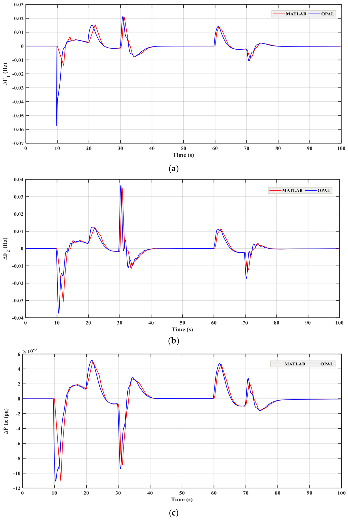
Figure 2. Nonlinear turbine model of GRC.
Energies 19 03601 g002
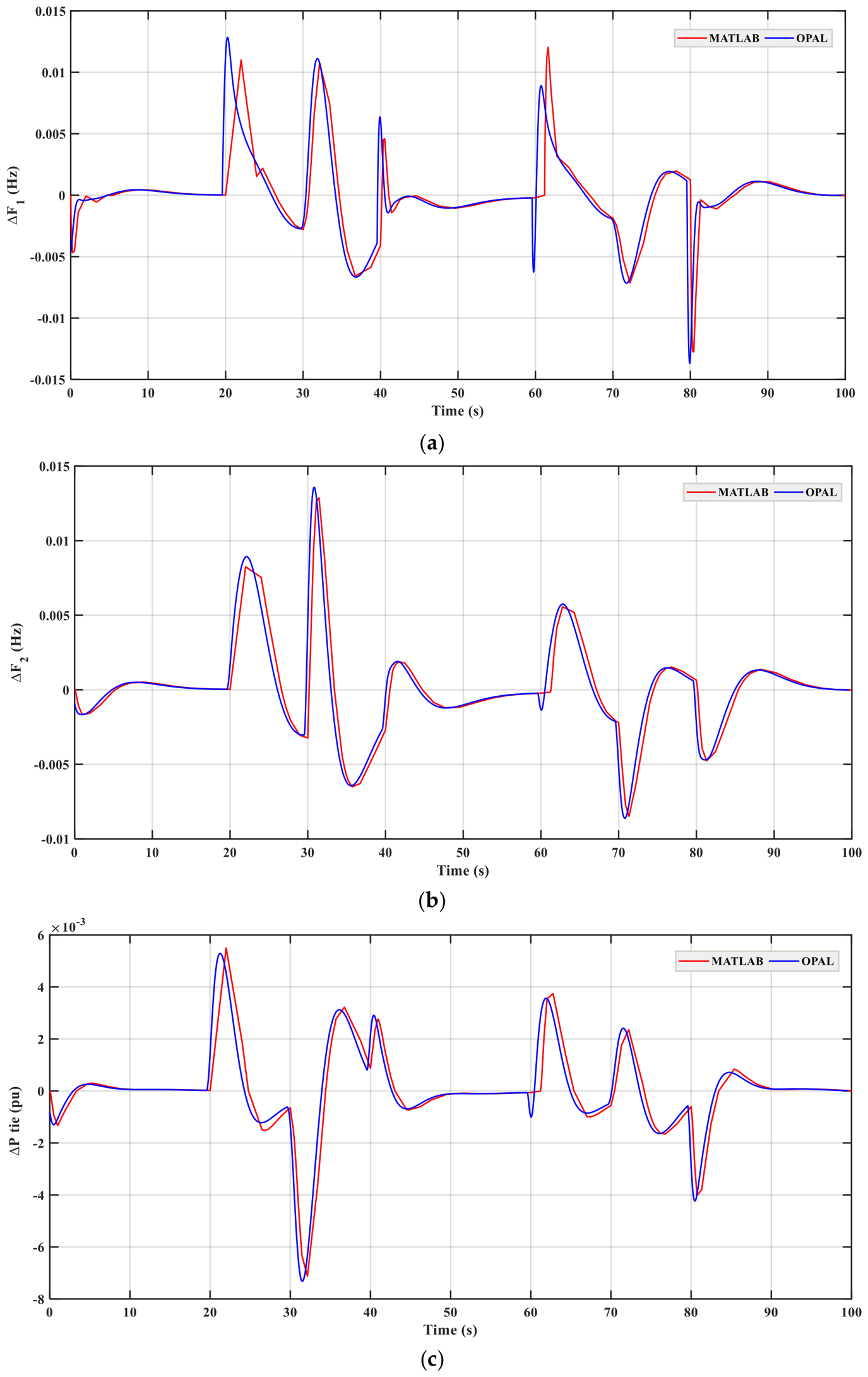
Figure 3. Block diagram of a two-area PS with RES integration.
Energies 19 03601 g003
Figure 4. Block diagram of a two-area PS with RES and ESS integration.
Energies 19 03601 g004
Figure 5. Block diagram of fluctuating PV model.
Energies 19 03601 g005
Figure 6. Block diagram of wind power of WT.
Energies 19 03601 g006
Figure 7. Block diagram of NREL 5 MW WT.
Energies 19 03601 g007
Figure 8. Block diagram of VRFB model.
Energies 19 03601 g008
Figure 9. Block diagram of SMES model.
Energies 19 03601 g009
Figure 10. Block diagram of HAFC model.
Energies 19 03601 g010
Figure 11. Block diagram of TDn(1+PIDn) controller.
Energies 19 03601 g011
Figure 12. Structure of hybrid PS with controller and optimization.
Energies 19 03601 g012
Figure 13. PKO flowchart.
Energies 19 03601 g013
Figure 14. Boxplot of PKO, GWO, and PSO using proposed controller.
Energies 19 03601 g014
Figure 15. Convergence profiles of PKO, GWO, and PSO using proposed controller.
Energies 19 03601 g015
Figure 16. System response for case 1 scenario 1. (a) ΔF1, (b) ΔF2, and (c) ΔPtie.
Energies 19 03601 g016aEnergies 19 03601 g016b
Figure 17. Comparison of system response between case 1 scenario 2 and scenario 3. (a) ΔF1, (b) ΔF2, and (c) ΔPtie.
Energies 19 03601 g017
Figure 18. Uniform solar and wind power profile.
Energies 19 03601 g018
Figure 19. System response for case 2 scenario 1. (a) ΔF1, (b) ΔF2, and (c) ΔPtie.
Energies 19 03601 g019
Figure 20. Random solar and wind power profile.
Energies 19 03601 g020
Figure 21. System response for case 2 scenario 2. (a) ΔF1, (b) ΔF2, and (c) ΔPtie.
Energies 19 03601 g021aEnergies 19 03601 g021b
Figure 22. Random load-change profile.
Energies 19 03601 g022
Figure 23. System response for case 2 scenario 3. (a) ΔF1, (b) ΔF2, and (c) ΔPtie.
Energies 19 03601 g023
Figure 24. System response for case 2 scenario 4. (a) ΔF1, (b) ΔF2, and (c) ΔPtie.
Energies 19 03601 g024
Figure 25. Comparison of system response between scenario 1 in case 2 and case 3. (a) ΔF1, (b) ΔF2, and (c) ΔPtie.
Energies 19 03601 g025
Figure 26. Comparison of system response between scenario 2 in case 2 and case 3. (a) ΔF1, (b) ΔF2, and (c) ΔPtie.
Energies 19 03601 g026aEnergies 19 03601 g026b
Figure 27. Comparison of system response between scenario 3 in case 2 and case 3. (a) ΔF1, (b) ΔF2, and (c) ΔPtie.
Energies 19 03601 g027
Figure 28. Comparison of system response between scenario 4 in case 2 and case 3. (a) ΔF1, (b) ΔF2, and (c) ΔPtie.
Energies 19 03601 g028aEnergies 19 03601 g028b
Figure 29. Experimental setup for real-time simulation using an OPAL-RT simulator.
Energies 19 03601 g029
Figure 30. Comparison of system response between MATLAB and OPAL for case 1 scenario 1. (a) ΔF1, (b) ΔF2, and (c) ΔPtie.
Energies 19 03601 g030
Figure 31. Comparison of system response between MATLAB and OPAL for case 2 scenario 1. (a) ΔF1, (b) ΔF2, and (c) ΔPtie.
Energies 19 03601 g031
Figure 32. Comparison of system response between MATLAB and OPAL for case 3 scenario 3. (a) ΔF1, (b) ΔF2, and (c) ΔPtie.
Energies 19 03601 g032
Table 1. Summary of literature review and proposed methodology on LFC.
ArticleControllerOptimization AlgorithmNo. of AreasRESESSKey Findings
[10]MPC-LQGCOA1-area and
2-area
(thermal non-reheat)
WT-COA-MPC-LQG delivers lower-frequency/tie-line deviations and faster settling under load disturbances and varying wind penetration, outperforming integral/MPC and PSO/GWO/ALO-tuned counterparts
[12]I-SMCGTO1-area
(microgrid
Wind-diesel)
WT-GTO-I-SMC improves frequency regulation in a wind–diesel autonomous microgrid, yielding smaller frequency deviations, shorter settling times, and lower integral error indices
[21]Fuzzy PIDGSA2-area
(thermal reheat)
--GSA-tuned PID-Fuzzy for a two-area reheat thermal system yields smaller frequency/tie-line deviations and lower integral error indices, outperforming PSO- and ABC-tuned counterparts under severe load disturbances
[27]FOPID-FOPICGO2-area (thermal non-reheat,
thermal reheat-hydro-gas)
and 3-area
(thermal-thermal-hydro)
--GO-FOPID-FOPI decreases deviation magnitudes and faster return to steady state across four IPS test systems: two-area non-reheat (±GDB), two-area reheater-hydro-gas multi-unit, and three-area hydrothermal with GRC, outperforming recent soft-computing controllers under modeled nonlinearities
[30]PD-PIDBA3-area
(thermal reheat)
--BA-PD–PID on a multi-area thermal system with single-reheat units and GRC delivers smaller frequency/tie-line deviations and quicker recovery than PI/PID, BA tuning outperforms GA/BF alternatives
[31]FTIDF-(1+I)WHO1-area
(microgrid
solar-wind-diesel)
PV-WTFESSWHO-FTIDF-(1+I) for an islanded microgrid (PV + WTG + diesel + flywheel ESU) achieves lower-frequency excursions and faster recovery than conventional alternatives under RES variability and load changes
[32]FO-ANFISADIWACO3-area
(thermal reheat)
PV-WT-FO-ANFIS (2-input & 3-input) for three-area RES system, trained from FOPI-FOPIDN (ADIWACO-tuned) data; 3-input FO-ANFIS achieves lower settling in area-1 with minimal over/undershoot, and near-zero tie-line overshoot/undershoot. Robust under GDB, delay and parameter variations (lowest integral error indices across scenarios besting FOPI-FOPIDN and IO-ANFIS variants)
[36]PI-TDFSSA1-area
(diesel-solar-wind-fuel cell-aqua electrolyzer)
PV-WTBESS-FESS-UCSSA-PI-TDF for a hybrid power system achieves lower frequency excursions and error indices than SSA-tuned PI/PID/TID/TIDF/P-TIDF comparators; validation under GRC nonlinearity, subsystem switching (BESS/FESS/diesel on/off), and parameter variations shows robust, less-sensitive performance
[37]PIDMOMSA2-area
(thermal non-reheat)
PV-WTEVMOMSA-PID for an interconnected microgrid with RESs + EVs markedly attenuates frequency oscillations and tie-line power fluctuations, outperforming PSO/MPA/GA, with faster transient response and improved stability across scenarios
[38]PIDGJO2-area
(thermal-hydro-nuclear,
thermal-gas)
PV-WTSMESGJO-PID on a two-area multi-source system: thermal, hydro, nuclear, gas, wind, and PV delivers smaller frequency & tie-line excursions versus PSO, WOA, SSA, ALO, Harris’ hawks, and TLBO, robustness is verified under variable step loads, parameter variations, and nonlinearities (GRC, GDB), stability margins are verified by frequency-response analysis, with fewer tuning iterations
[41]FOTIDD2MOA2-area
(marine bio-diesel-sea wave energy)
PV-WTBESS-CESMOA-FOTIDD2 on a two-area diverse (sea-wave, PV, wind, biodiesel, BESS, and CES) with communication delay achieves lower frequency and tie-line excursions, faster settling, and improved damping than PID baselines, while MOA consistently surpasses SCA/FOA/GWO in tuning effectiveness and robustness
[42]TDn(1+PI)BDGOA2-area
(PV-thermal reheat)
PV-The BDGOA-TDn(1+PI) proposed design retains stability and tracking quality under delays and uncertainty and outperforms standard controllers in reducing frequency and tie-line power fluctuations
[48]PIDGOA-PSO1-area (thermal non-reheat-solar-wind-EV) and 2-area (thermal non-reheat)PV-WTEVStandalone PSO exhibits premature convergence and local optima entrapment in renewable-integrated LFC; the proposed GOA-PSO hybrid exploits GOA’s exploratory strength to escape local optima, achieving marked reductions in overshoot, undershoot, and settling time over conventional PSO-PID
[49]FOPIDMPO2-area and 4-area (thermal reheat-hydro-wind)WTRFB-HAFCConventional metaheuristics suffer limited population diversity leading to premature convergence; the proposed MPO avoids trapping in local optima taking advantage over GWO through memory-based election and random exploration strategies, reducing ITAE by 8.023% and 20.071% in two- and four-microgrid systems, respectively
[50]FOPIDASIA3-area (thermal non-reheat-wind-hydro)WT-GA, GWO, SCIA, and ASIA are benchmarked comparatively for PID/FOPID tuning in three-area LFC; ISE-based GA/SCIA and ITSE-based GWO/ASIA-tuned FOPID controllers deliver superior regulation under parameter perturbations and varying load conditions; ASIA/SCIA are highlighted against GA/GWO
ProposedTDn(1+PIDn)PKO2-area
(thermal non-reheat)
PV-WTVRFB-SMES-HAFCPKO-TDn(1+PIDn) on a two-area system (area 1: thermal non-reheat, PV, VRFB, SMES, area 2: thermal non-reheat, WT, VRFB, HAFC) achieves lower frequency and tie-line excursions, faster settling, and improved damping than PID baselines, while PKO consistently surpasses GWO/PSO in tuning effectiveness and robustness; validating the results with OPAL-RT
Table 2. Nominal values of system parameters.
ParametersValuesParametersValues
F60 Hza12−1
Pr1 = Pr22000 MWB1 = B20.425 pu MW/Hz
PD1000 MWR12.4 Hz/pu MW
GRC±0.05 or ±0.025KP1 = KP2120
TP1 = TP220 sTT1 = TT20.3 s
T120.545 TG1 = TG20.08 s
Table 3. Values of uniform model of PV and WT.
ParametersValuesParametersValues
KPV1 KWT1
TPV1.3 sTWT1.5 s
Table 4. Values of ESS parameters.
ParametersValuesParametersValues
KRFB1 TdRFB0 s
TcRFB0.3 sKSMES0.2035
TSMES0.03 sT10.2333 s
T20.016 sT30.7087 s
T40.2481 sKn0.6
Kae0.002 Kfc0.01
Tae0.5 sTfc4 s
Table 5. Optimal ITAE and parameters of proposed and other controllers.
Algorithm-
Controller
ITAEAreaParameters
K T K D 1 n N K P K I K D D NNλμPWDW
PKO-TDn(1+PIDn)0.0373Area 11.960.6270.9921.0061.96602286----
Area 201.9990.694100021.9851.99464----
GWO-TDn(1+PIDn)0.0544Area 120.2370.001117.90.18220.2610.8----
Area 21.540.6860.41911.960.9200.4171.94786----
PSO-TDn(1+PIDn)0.05550Area 120.0470947.50.30920.3785.5----
Area 221.3700.427727.51.6570.3680.08406----
PKO-PID0.12696Area 1-0.394--1.0842------
Area 2-0.543--1.9970.057------
GWO-PID0.12701Area 1-0.399--1.0862------
Area 2-0.562--20.246------
PSO-PID0.12702Area 1-0.402--1.0922------
Area 2-0.561--1.9810.156------
DSA-FOPID [73]0.0778Area 1-0.467--2.0332.999--1.00071.0517--
Area 2-NA--NANA--NANA--
WOA-tuned 2DOF TIDF [74]0.0734Area 13.881.8560.105227.8-3.963----1.2430.423
Area 2NANANANA-NA----NANA
WOA-tuned TIDF [74]0.1167Area 11.400.3770.111230.9-1.877------
Area 2NANANANA-NA------
EPSDE-PID [39]0.1497Area 1-0.388--0.8591.773------
Area 2-1.011--1.0410.165------
CLPSO-PID [39]0.1569Area 1-0.384--1.0141.705------
Area 2-0.583--1.7200.428------
HPSO-PS tuned fuzzy PI [52]0.1438Area 1----0.9850.559------
Area 2----0.9330.720------
PS-tuned fuzzy PI [52]0.6334Area 1----0.7310.647------
Area 2----0.4500.547------
PSO-tuned fuzzy PI [52]0.4470Area 1----0.5080.510------
Area 2----0.8170.794------
Note: NA indicates that the corresponding source does not report parameters for Area 2.
Table 6. Limits of proposed controller parameters.
Gains K T K D 1 n N K P K I K D D NN
Lower limit (min)00010001
Upper limit (max)22110002221000
Table 7. Statistical analysis using the proposed controller.
AlgorithmPSOGWOPKO
Best0.0555030.0544150.037309
Worst0.109530.0562910.057297
Mean0.06824280.05530710.0530751
Standard deviation0.0215652850.00059670.006091139
Table 8. Summary of tested dynamic scenarios.
Case/ScenarioLoad DisturbanceRES ProfileESS IntegrationNonlinearity/
Uncertainty Source
C1-S1Step +0.1 pu in Area 1 (t = 0)---
C1-S2Step +0.05 pu in Area 1 (t = 0)--GRC ±0.05
GDB
CTD 0.1 s
C1-S3Step +0.05 pu in Area 1 (t = 0)--GRC ±0.025
GDB
CTD 0.1 s
C2-S1Step +0.1 pu in Area 1 (t = 10 s)
Uniform PV in Area 1
Uniform WT in Area 2
-UniformRES
C2-S2Step +0.1 pu in Area 1 (t = 10 s)
Random PV in Area 1
Random WT in Area 2
-RandomRES
C2-S3Random in Area 1
Uniform PV in Area 1
Uniform WT in Area 2
-UniformRES
Randomload
C2-S4Random in Area 1
Random PV in Area 1
Random WT in Area 2
-RandomRES
Randomload
C3-S1: C3-S4As C2-S1: C2-S4As C2-S1: C2-S4
VRFB and SMES in Area 1
VRFB and HAFC in Area 2
Uniformor
RandomRES
Randomload
C4
(Validation by OPAL-RT)
tested scenarios:
C1-S1
C-S1
C3-S3
As caseAs caseAs case
Table 9. ITAE and parameters of controllers with optimizations in case 1 scenario 1.
Algorithm ControllerITAEAreaParameters
K T K D 1 n N K P K I K D D NN
PKO-TDn(1+PIDn)0.037309Area 11.96740.6274780.992744061.00668121.966202802285.75433
Area 201.99997040.69481776100021.98547471.9989607463.98808
GWO-TDn(1+PIDn)0.054415Area 120.23757880.000853708117.90920.182884120.263937110.74717
Area 21.54970.686340.419554411.961160.92004380.41738511.942215785.5651
PSO-TDn(1+PIDn)0.055503Area 120.047352230947.50540.309834920.376052485.46221
Area 221.3705240.4270762727.51131.6571960.36873190.0822369406.3412
PKO-PID0.12696Area 1-0.39474--1.0842--
Area 2-0.54378--1.9970.057774--
GWO-PID0.12701Area 1-0.399--1.08692--
Area 2-0.5627--20.24698--
PSO-PID0.12702Area 1-0.40273--1.0922--
Area 2-0.56175--1.98120.15687--
Table 10. Comparative performance analysis in case 1 scenario 1.
Algorithm Controller F 1 F 2 P t i e
USOS T S (s)USOS T S (s)USOS T S (s)
PKO-TDn(1+PIDn)−0.06240.0010274.573−0.016790.00014823.303−0.007290.00004853.302
GWO-TDn(1+PIDn)−0.07340.0014284.604−0.026700.00000594.103−0.011470.00000624.292
PSO-TDn(1+PIDn)−0.07440.0027594.944−0.029000.00000293.896−0.011730.00001104.296
PKO-PID−0.11370.0063896.208−0.061750.00007533.938−0.022430.00002364.403
GWO-PID−0.11310.0057356.267−0.061360.00007813.997−0.022320.00002394.397
PSO-PID−0.11300.0052386.253−0.061190.00007954.222−0.022150.00002474.395
Table 11. Sensitivity analysis using the proposed method in case 1 scenario 1.
System
Parameters
Change (%)ITAE F 1 F 2 P t i e
USOS T S (s)USOS T S (s)USOS T S (s)
K P +250.03704−0.06850.0009844.4−0.016610.0001553.2−0.007160.0000383.25
−250.03769−0.0550.0012554.8−0.016610.0001353.4−0.007310.0000673.35
T P +250.03764−0.05710.0011984.7−0.016720.0001373.5−0.007330.0000633.4
−250.03707−0.07030.0010494.5−0.01650.0001573.2−0.007110.0000353.22
T 12 +250.03461−0.06150.000554.4−0.01930.0001683.15−0.008370.00005763.21
−250.04304−0.06350.0017624.75−0.01370.0001053.55−0.005960.00003053.46
Table 12. Comparison of ITAE and parameters of the proposed method between case 1 scenario 2 and scenario 3.
ScenarioAlgorithm ControllerITAEAreaParameters
K T K D 1 n N K P K I K D D NN
2PKO-TDn(1+PIDn)1.0633Area 10.383400.99737222.63330.533600929.609
Area 20.028700.85564524.2251.96910.056510.1418239.805
3PKO-TDn(1+PIDn)1.4269Area 10.613220.00675802.29390.60010.563830.35423527.522
Area 20.05840.260197.21550.08430.113290.80599607.188
Table 13. Comparative performance analysis between case 1 scenario 2 and scenario 3.
ScenarioAlgorithm Controller F 1 F 2 P t i e
USOS T S (s)USOS T S (s)USOS T S (s)
2PKO-TDn(1+PIDn)−0.12790.03078.25−0.12130.043117.72−0.03540.0068448.32
3PKO-TDn(1+PIDn)−0.14020.06428.632−0.1710.043218.75−0.038020.0086829.44
Table 14. ITAE and parameters of controllers with optimizations in case 2 all scenarios.
ScenarioAlgorithm ControllerITAEAreaParameters
K T K D 1 n N K P K I K D D NN
1PKO-TDn(1+PIDn)21.9239Area 10.9930.5700.422534.09410.97911
Area 20.9880.1660.928110.9480.766900.686
GWO-TDn(1+PIDn)23.6983Area 110.6100.359183.02310.9930.488845.174
Area 210.3850.7422.1170.7410.9900.049642.868
PSO-TDn(1+PIDn)26.7529Area 10.9920.4840.946240.8670.7000.8460.911454.232
Area 20.9940.1491757.8790.73600.338643.089
PKO-PID37.0438Area 1-0.938--0.9451--
Area 2-0.305--0.7291--
GWO-PID38.2655Area 1-0.627--0.3861--
Area 2-0.533--0.3160.997--
PSO-PID40.7485Area 1-0.260--0.5510.829--
Area 2-0.275--0.0550.995--
2PKO-TDn(1+PIDn)11.5592Area 110.4790.9721.0110.9820.0060.999318.155
Area 210.9760.445695.5540.9740.9660.145783.744
GWO-TDn(1+PIDn)16.1475Area 10.8890.1940.319409.5930.4340.9470.713270.974
Area 210.9270.630253.1130.9760.4570.49456.294
PSO-TDn(1+PIDn)15.2312Area 110.1860.587833.54710.5180.757862.131
Area 20.9880.7490.545502.1820.8070.8050.107531.774
PKO-PID20.5254Area 1-0.989--0.9991--
Area 2-1--0.9991--
GWO-PID21.4565Area 1-0.363--0.4021--
Area 2-0.741--0.9391--
PSO-PID23.2232Area 1-0.665--0.3771--
Area 2-0.684--0.6391--
3PKO-TDn(1+PIDn)28.2608Area 110.3850.68310.9350.4740.7381000
Area 210.8250.611591.675110.384484.001
GWO-TDn(1+PIDn)30.9221Area 110.7550.384162.2410.2370.9150.183524.869
Area 20.9710.3230.803321.5350.9700.6650.773592.184
PSO-TDn(1+PIDn)33.7697Area 110.0460.348171.6140.0500.9080.422492.020
Area 20.9900.2880.849374.1780.4000.90.8961
PKO-PID39.7584Area 1-0.277--0.9101--
Area 2-0.696--0.9851--
GWO-PID44.4464Area 1-0.315--0.2961--
Area 2-0.332--−0.1641--
PSO-PID46.0625Area 1-0.315--0.2040.995--
Area 2-0.467--0.7260.828--
4PKO-TDn(1+PIDn)16.5372Area 10.9610.8490.349823.58310.9970.537331.455
Area 20.9970.9990.468834.8490.9640.9410.996423.283
GWO-TDn(1+PIDn)19.8685Area 110.2340.604408.7230.9560.5050.398910.161
Area 20.9660.5300.067105.3330.9940.7540.152274.736
PSO-TDn(1+PIDn)20.2288Area 110.7980.585660.4370.8670.4040.331112.168
Area 20.9990.90.462592.2840.4590.90.687182.425
PKO-PID27.748Area 1-0.999--11--
Area 2-1--11--
GWO-PID28.927Area 1-0.386--0.5341--
Area 2-0.869--0.9280.957--
PSO-PID29.1459Area 1-0.553--0.6181--
Area 2-0.748--0.81151--
Table 15. Comparative performance analysis in case 2 all scenarios.
ScenarioAlgorithm Controller F 1 F 2 P t i e
USOSUSOSUSOS
1PKO-TDn(1+PIDn)−0.013890.02059−0.030620.03483−0.011090.00501
GWO-TDn(1+PIDn)−0.024890.01935−0.033150.03497−0.012490.00505
PSO-TDn(1+PIDn)−0.025520.04314−0.035990.04380−0.013660.01083
PKO-PID−0.035020.03192−0.051940.04090−0.019710.00815
GWO-PID−0.044030.03782−0.065230.04545−0.025070.01020
PSO-PID−0.037770.04530−0.071840.05265−0.026250.01036
2PKO-TDn(1+PIDn)−0.10220.01419−0.044520.01174−0.018230.001620
GWO-TDn(1+PIDn)−0.081230.01749−0.048650.01463−0.020140.002504
PSO-TDn(1+PIDn)−0.081840.01733−0.049800.01272−0.019470.002220
PKO-PID−0.078550.01997−0.043040.01620−0.017420.003231
GWO-PID−0.128500.02589−0.078160.02021−0.029010.003435
PSO-PID−0.099800.02528−0.062800.01945−0.023570.004048
3PKO-TDn(1+PIDn)−0.031170.02655−0.013700.01841−0.007310.00643
GWO-TDn(1+PIDn)−0.017700.02095−0.012820.02613−0.009660.00698
PSO-TDn(1+PIDn)−0.039230.03146−0.023410.03013−0.009260.00907
PKO-PID−0.039450.03302−0.022010.03238−0.011510.00908
GWO-PID−0.040110.04728−0.026600.06134−0.017840.01121
PSO-PID−0.040160.03868−0.025860.03816−0.013130.01222
4PKO-TDn(1+PIDn)−0.013920.01128−0.012640.00793−0.002720.00292
GWO-TDn(1+PIDn)−0.028290.01708−0.020730.01209−0.005240.00431
PSO-TDn(1+PIDn)−0.017340.01391−0.015760.00909−0.003410.00358
PKO-PID−0.025750.01686−0.019650.01485−0.004120.00429
GWO-PID−0.039800.02400−0.028410.01581−0.006860.00602
PSO-PID−0.034600.02047−0.025960.01697−0.005630.00532
Table 16. Comparison of ITAE and parameters of the proposed method in scenario 1 for case 2 and case 3.
ESS
Contribution
Algorithm ControllerITAEAreaParameters
K T K D 1 n N K P K I K D D NN
Without ESSsPKO-TDn(1+PIDn)21.9239Area 10.9930.5700.422534.09410.97911
Area 20.9880.1660.928110.9480.766900.686
With ESSsPKO-TDn(1+PIDn)20.9967Area 10.9990.9420.4531.0140.9990.9990.311319.381
Area 20.99800.812166.9090.9980.9910.8491
Table 17. Comparative performance analysis of scenario 1 in case 2 and case 3.
ESS ContributionAlgorithm Controller F 1 F 2 P t i e
USOSUSOSUSOS
Without ESSsPKO-TDn(1+PIDn)−0.013890.02059−0.030620.03483−0.011090.00501
With ESSsPKO-TDn(1+PIDn)−0.007830.01283−0.021380.01752−0.012060.00508
Table 18. Comparison of ITAE and parameters of the proposed method in scenario 2 for case 2 and case 3.
ESS
Contribution
Algorithm ControllerITAEAreaParameters
K T K D 1 n N K P K I K D D NN
Without ESSsPKO-TDn(1+PIDn)11.5592Area 110.4790.9721.0110.9820.0060.999318.155
Area 210.9760.445695.5540.9740.9660.145783.744
With ESSsPKO-TDn(1+PIDn)9.3698Area 110.4900.9891.0970.99400.994562.589
Area 20.9990.9100.55110.8990.9990.932685.462
Table 19. Comparative performance analysis of scenario 2 in case 2 and case 3.
ESS ContributionAlgorithm Controller F 1 F 2 P t i e
USOSUSOSUSOS
Without ESSsPKO-TDn(1+PIDn)−0.10220.01419−0.044520.01174−0.018230.001620
With ESSsPKO-TDn(1+PIDn)−0.047090.009927−0.022290.007583−0.014160.002362
Table 20. Comparison of ITAE and parameters of the proposed method in scenario 3 for case 2 and case 3.
ESS
Contribution
Algorithm ControllerITAEAreaParameters
K T K D 1 n N K P K I K D D NN
Without ESSsPKO-TDn(1+PIDn)28.2608Area 110.3850.68310.9350.4740.7381000
Area 210.8250.611591.675110.384484.001
With ESSsPKO-TDn(1+PIDn)22.5031Area 1110.476110.9880.234586.983
Area 20.9650.2340.76662.5071111000
Table 21. Comparative performance analysis of scenario 3 in case 2 and case 3.
ESS ContributionAlgorithm Controller F 1 F 2 P t i e
USOSUSOSUSOS
Without ESSsPKO-TDn(1+PIDn)−0.031170.02655−0.013700.01841−0.007310.00643
With ESSsPKO-TDn(1+PIDn)−0.012760.01206−0.008490.01288−0.007120.005499
Table 22. Comparison of ITAE and parameters of the proposed method in scenario 4 for case 2 and case 3.
ESS
Contribution
Algorithm ControllerITAEAreaParameters
K T K D 1 n N K P K I K D D NN
Without ESSsPKO-TDn(1+PIDn)16.5372Area 10.9610.8490.349823.58310.9970.537331.455
Area 20.9970.9990.468834.8490.9640.9410.996423.283
With ESSsPKO-TDn(1+PIDn)12.3843Area 10.9890.9750.6341.0040.9950.9990.649986.024
Area 20.9950.9910.29344.3560.96910.40193.692
Table 23. Comparative performance analysis of scenario 4 in case 2 and case 3.
ESS ContributionAlgorithm Controller F 1 F 2 P t i e
USOSUSOSUSOS
Without ESSsPKO-TDn(1+PIDn)−0.013920.01128−0.012640.00793−0.002720.00292
With ESSsPKO-TDn(1+PIDn)−0.013550.007986−0.0081290.005345−0.002660.00266
Table 24. Quantitative comparison between MATLAB and OPAL-RT simulation results.
Case/Scenario F 1 F 2 P t i e
Max |Error|RMSENRMSE (%)Max |Error|RMSENRMSE (%)Max |Error|RMSENRMSE (%)
C1-S10.00530.000891.40.00150.000181.10.000660.000081.1
C2-S10.0570.004613.240.02950.00395.920.00940.00116.98
C3-S30.0150.00218.530.00820.00115.350.00280.000645.04
Disclaimer/Publisher’s Note: The statements, opinions and data contained in all publications are solely those of the individual author(s) and contributor(s) and not of MDPI and/or the editor(s). MDPI and/or the editor(s) disclaim responsibility for any injury to people or property resulting from any ideas, methods, instructions or products referred to in the content.